IEEE TRANSACTIONS ON KNOWLEDGE AND DATA … · We employ energy-efficient ... query processing, wireless sensor networks. ... more reliable message delivery in the lossy sensor network

Nonthreshold-Based Event Detection for3D Environment Monitoring in Sensor Networks

Mo Li, Member, IEEE, Yunhao Liu, Senior Member, IEEE, and Lei Chen, Member, IEEE

Abstract—Event detection is a crucial task for wireless sensor network applications, especially environment monitoring. Existing

approaches for event detection are mainly based on some predefined threshold values and, thus, are often inaccurate and incapable of

capturing complex events. For example, in coal mine monitoring scenarios, gas leakage or water osmosis can hardly be described by

the overrun of specified attribute thresholds but some complex pattern in the full-scale view of the environmental data. To address this

issue, we propose a nonthreshold-based approach for the real 3D sensor monitoring environment. We employ energy-efficient

methods to collect a time series of data maps from the sensor network and detect complex events through matching the gathered data

to spatiotemporal data patterns. Finally, we conduct trace-driven simulations to prove the efficacy and efficiency of this approach on

detecting events of complex phenomena from real-life records.

Index Terms—Distributed applications, data compaction and compression, query processing, wireless sensor networks.

Ç

1 INTRODUCTION

WIRELESS sensor networks (WSNs) have been widelystudied for environment monitoring. In such mon-

itoring applications, automatically detecting events is quiteessential, e.g., for detecting vehicles or forest fires. Cur-rently, the typical event detection method [12] relies ondecisions made at the sensor node(s) based on predefineddata thresholds for normal environments. The rationalebehind such threshold-based approaches is that whenevents occur, there will be detectable changes in environ-mental data. Thus, an event can be captured once theobserved sensory data exceed the predefined thresholds.

Our motivating scenario comes from the field study in a

coal mine [15], where environment surveillance is carried out

to ensure miners’ safety. The amount of oxygen, gas, dust,

temperature, humidity, and watery regions are monitored in

a 3D space of underground tunnels in the mine. Several event

detection tasks are essential to secure the safety of the miners,

such as detecting gas leakage, oxygen-enriched spots, and water

seepage. Gas leakage often occurs when the digging machines

expose a source of gas in the mining process, and it often

leads to a local increase in gas density. If a certain district of

gas accumulates to critical explosive density, explosions

could occur. Oxygen-enriched spots exist at the ventilative

places where high oxygen density creates healthy environ-

mental conditions for human beings. Indicating such areas

provides important guidelines for the miners patrolling in

the coal mine. Water seepage brings water into the coal mine

tunnels, which corrodes the tunnel surfaces and threatens

the tunnel’s structural integrity.

The events described above share the common char-acteristics that their occurrence results in trends in thedevelopment of environmental data rather than someinstantaneous overrun of specified thresholds in individualsensor nodes. Hence, the threshold-based approaches workwell for detecting simple events, but the complex eventswith spatiotemporal variety in the environment can hardlybe captured by a simple cutoff method. An integrative viewof the environment has to be established to extract thefeatures of such events. For example, gas leakage usuallyleads to an expanding area of high gas density over time,which spatially follows a degrading form where the gasdensity decreases from the source of the leak. The waterseepage can be categorized as a “fault event” with anapparent observation on the advances of the frontierbetween the dry area and the flooded area.

In order to accurately detect complicated events, we needa nonthreshold-based event detection approach. We intendto describe complex phenomena with certain spatiotempor-al data patterns and detect events through matching thegathered data to such data patterns. The challenges for sucha design are as follows: First, differing from threshold-basedapproaches, the environment data map has to be continu-ously maintained from real-time sensor readings, whileconserving energy for battery-powered sensors [5], [6], [23],[25], [27] is a very critical issue. We need to restrain the datatraffic and maintain the data map in an energy-efficientmanner. Second, the communication quality of WSNs ispoor, especially in the underground monitoring environ-ments, such as a coal mine. We have to develop robustmethods of data map construction so that the accuracy ofthe obtained data map could be preserved in a high loss ratenetwork. Third, the 3D monitoring field raises nontrivialissues in abstracting the environment, which are not facedby previous works in 2D cases. Efficient data structures andmodeling methods are required in a point of 3D view.

In this paper, we propose a 3D gradient data map usingthe space orthogonal polyhedra (OP) model. We build a

IEEE TRANSACTIONS ON KNOWLEDGE AND DATA ENGINEERING, VOL. 20, NO. 12, DECEMBER 2008 1699

. The authors are with the Department of Computer Science and Engineering,Hong Kong University of Science and Technology, Clear Water Bay,Kowloon, Hong Kong. E-mail: {limo, liu, leichen}@cse.ust.hk.

Manuscript received 25 May 2007; revised 7 Feb. 2008; accepted 15 May2008; published online 2 June 2008.For information on obtaining reprints of this article, please send e-mail to:[email protected], and reference IEEECS Log Number TKDE-2007-05-0236.Digital Object Identifier no. 10.1109/TKDE.2008.114.

1041-4347/08/$25.00 � 2008 IEEE Published by the IEEE Computer Society

Authorized licensed use limited to: IEEE Xplore. Downloaded on January 13, 2009 at 03:39 from IEEE Xplore. Restrictions apply.

multipath routing architecture to provide robust datadelivery for the map construction. Instead of directlyrouting raw data to the sink before processing, a novel3D aggregation algorithm is designed for map constructionand update. We demonstrate the efficacy and efficiency ofthe proposed approach in trace-driven simulations usingsynthetic data sets derived from the raw data collected inour study in the real coal mine environment.

The rest of this paper is organized as follows: We brieflyreview the related work in Section 2. In Section 3, wedescribe the network architecture and construction of thegradient data map. The aggregation criteria and incre-mental data map construction techniques are also intro-duced. In Section 4, we describe the event feature patternsand illustrate how pattern-based event detection is per-formed on the data map. Experimental studies of ourapproach are given in Section 5. Finally, we conclude thiswork in Section 6.

2 RELATED WORK

Event detection remains an essential task in various WSNapplications. There are a number of recent works on event-oriented query processing in sensor networks. TheCOUGAR project [3] introduces a sensor database systemand deals with three types of event queries: historicalqueries, snapshot queries, and long-running queries. Thesystem employs threshold-based detection logic and en-capsulates it into a set of asynchronous functions providedfor users. Directed Diffusion [14] aims at addressing theevent-based real-time queries by diffusing different eventinterests into the monitoring network and letting sensorsreport when occurrences of some specified events aredetected. The Directed Diffusion approach does not explorethe spatial or temporal correlations among the sensory data,and it relies on individual reports of sensor nodes accordingto the disseminated event interests. TinyDB [12] defines theevent by a composition of various specified attributethresholds. The event detection is carried out by comparingsensory readings of attributes with predetermined thresh-old values. TinyDB provides a distributed mapping methodto construct contour maps of sensor network readings.Differing from our approach, the mapping process inTinyDB is only done in 2D fields and their work doesnot aim to provide event detection based on the dataspatiotemporal patterns. DSWare [16] explores the correla-tion among different sensor observations for event detec-tion. Events are grouped into two different types: atomicevents and compound events. Confidence functions areemployed to address compound events. Above works allfocus on 2D scenarios.

In-network data aggregation has been intensively studiedas an effective method to provide energy-efficient datacollection [4], [17], [18], [19], [21]. LEACH [11] protocolconstructs clustering hierarchy on the network and achievesdata fusion at the cluster heads to reduce transmittedinformation. By rotating the cluster heads, energy dissipa-tion is evenly distributed over the network. The TAGapproach [19] builds a routing tree in the sensor networkand statistical data are aggregated in the intermediate nodes.In [17], network tomography techniques have been applied

to solve the problem of loss inference in data aggregation.Different from the approaches above, our approach exploresthe spatial correlations on the sensory data and achieves

data aggregation through the combination of OP in thegradient data maps. Recently proposed contour mappingmethods [12], [20], [24] share similar ideas with this work in

visualizing the monitored fields for event detection. Whilethose works utilize aggregation-based approaches to effi-ciently approximate the 2D field in contour maps, theyprovide no means to extend for 3D scenarios.

The multipath routing strategy has recently been

suggested to provide robust data deliveries in sensor

networks. Robust aggregation on it needs duplicate-insen-

sitive data structures to carry information [7], [22]. In our

work, we propose the space OP model as such a duplicate-

insensitive data structure.

3 THREE-DIMENSIONAL GRADIENT DATA MAP

CONSTRUCTION

This section is organized as follows: In Section 3.1, we

briefly describe the sensor network architecture and

deployment of sensors in a 3D space. Then, in Section 3.2,

we present the concept of 3D gradient data map. In

Section 3.3, we introduce the OP and describe how to

achieve in-network construction of the gradient data map

by the space OP model. Sections 3.4 and 3.5 describe the

aggregation criteria for the gradient data map construction

and its incremental update. Finally, in Section 3.6, we

extend our algorithm for random sensor deployments.

3.1 Network Architecture

In our coal mine monitoring scenario, sensor nodes are

assumed uniformly deployed in 3D monitoring space with

measured location information (later, we will release this

constraint to extend our work into random deployments).

This could be easily achieved by placing sensors along the

safety props in the tunnel. Fig. 1 shows the environment in

underground coal mine tunnels and the placement of

sensors in our underground prototype system previously

reported in [15]. A cubic grid can be established on this

network and each sensor node accounts for the environ-

ment sensing in the cubic cell it resides in (as shown in

Fig. 2a). The grid information is created at sink and

disseminated throughout the network. Each sensor node,

based on its location information, calculates the dimension

and coordinates of the cubic cell it resides in.The whole network is organized into multipath routing

architecture. Sensor nodes are divided into different levels

from the sink. The sensor nodes closer to the sink have lower

levels. For each sensor node, the one level lower nodes are

considered as parent neighbors, and the one level higher

nodes are treated as child neighbors. Each node forwards the

query messages originated in the sink to its child neighbors

and sends the report messages to its parent neighbors. Thus,

in the message relay process at each node, multirelayers are

triggered for message forwarding. By the means of multi-

path routing, message redundancy is provided to ensure a

more reliable message delivery in the lossy sensor network.

1700 IEEE TRANSACTIONS ON KNOWLEDGE AND DATA ENGINEERING, VOL. 20, NO. 12, DECEMBER 2008


The multipath routing architecture is constructed by a

two-phase initialization process, DIFFUSION and ECHO. In

the DIFFUSION phase, the sink originated indicator mes-

sage is flooded into the network. Each sensor node estimates

its hop count from the sink. When the DIFFUSION phase

completes, each sensor node gets its level and discovers its

parent neighbors and child neighbors. The ECHO phase is

triggered by the highest level sensor nodes, which are

farthest from the sink. ECHO messages are created by those

nodes and flooded in the network. Hence, the total level

count is captured by all the nodes and each node calculates

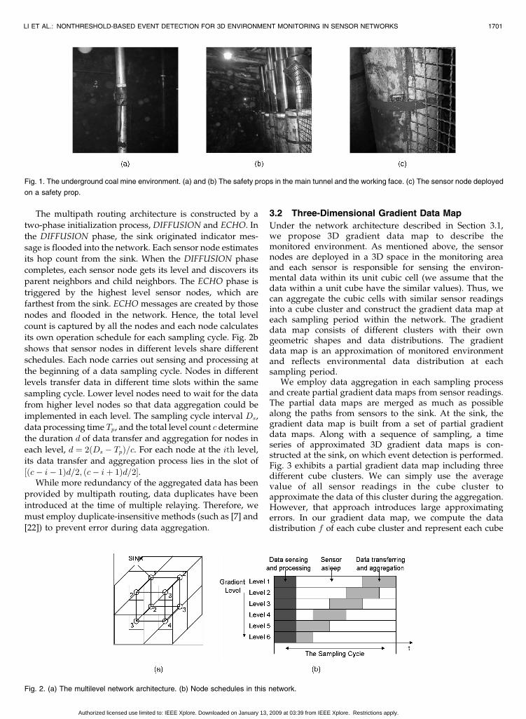
its own operation schedule for each sampling cycle. Fig. 2b

shows that sensor nodes in different levels share different

schedules. Each node carries out sensing and processing at

the beginning of a data sampling cycle. Nodes in different

levels transfer data in different time slots within the same

sampling cycle. Lower level nodes need to wait for the data

from higher level nodes so that data aggregation could be

implemented in each level. The sampling cycle interval Ds,

data processing time Tp, and the total level count c determine

the duration d of data transfer and aggregation for nodes in

each level, d ¼ 2ðDs � TpÞ=c. For each node at the ith level,

its data transfer and aggregation process lies in the slot of

½ðc� i� 1Þd=2; ðc� iþ 1Þd=2�.While more redundancy of the aggregated data has been

provided by multipath routing, data duplicates have been

introduced at the time of multiple relaying. Therefore, we

must employ duplicate-insensitive methods (such as [7] and

[22]) to prevent error during data aggregation.

3.2 Three-Dimensional Gradient Data Map

Under the network architecture described in Section 3.1,we propose 3D gradient data map to describe themonitored environment. As mentioned above, the sensornodes are deployed in a 3D space in the monitoring areaand each sensor is responsible for sensing the environ-mental data within its unit cubic cell (we assume that thedata within a unit cube have the similar values). Thus, wecan aggregate the cubic cells with similar sensor readingsinto a cube cluster and construct the gradient data map ateach sampling period within the network. The gradientdata map consists of different clusters with their owngeometric shapes and data distributions. The gradientdata map is an approximation of monitored environmentand reflects environmental data distribution at eachsampling period.

We employ data aggregation in each sampling processand create partial gradient data maps from sensor readings.The partial data maps are merged as much as possiblealong the paths from sensors to the sink. At the sink, thegradient data map is built from a set of partial gradientdata maps. Along with a sequence of sampling, a timeseries of approximated 3D gradient data maps is con-structed at the sink, on which event detection is performed.Fig. 3 exhibits a partial gradient data map including threedifferent cube clusters. We can simply use the averagevalue of all sensor readings in the cube cluster toapproximate the data of this cluster during the aggregation.However, that approach introduces large approximatingerrors. In our gradient data map, we compute the datadistribution f of each cube cluster and represent each cube

LI ET AL.: NONTHRESHOLD-BASED EVENT DETECTION FOR 3D ENVIRONMENT MONITORING IN SENSOR NETWORKS 1701

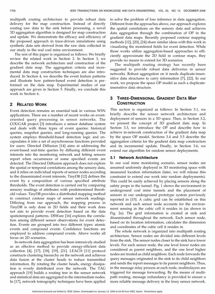
Fig. 1. The underground coal mine environment. (a) and (b) The safety props in the main tunnel and the working face. (c) The sensor node deployed

on a safety prop.

Fig. 2. (a) The multilevel network architecture. (b) Node schedules in this network.


cluster by the geometric structure, called space OP. Bymanipulating two parameters of OP, which can be simplytransmitted with little bandwidth, the sensor nodes arecollaborated to construct the gradient data map in an in-network manner. The key operations in the aggregationprocess are estimating the similarity of different OP andmerging the similar OP at each sensor node.

3.3 Space OP Model and Gradient MapConstruction

We use the space OP model to describe different cubeclusters. OP can capture the data distribution in 3D cubicspace and only requires few parameter settings. The OPwas first introduced in Constructive Solid Geometry (CSG).Aguilera and Ayala investigated the characteristics of OP[1] and presented the geometric models to represent OP aswell as some basic geometric operations, which aresummarized as follows:

Definition 3.1. OP are polyhedra with all faces oriented in threeorthogonal directions.

In OP, all planes and lines are parallel to threeorthogonal axes. The number of incident edges for eachvertex can be only three, four, or six, which is referred asV3, V4, or V6, respectively [1]. An Extreme Vertices (EV)model has been proposed to represent OP.

Definition 3.2. The EV model for OP is defined as a model thatonly stores all V3 vertices.

Aguilera and Ayala proved that the EV model is a validB-Rep model, i.e., it is complete and compact in the sense ofgeometry. Furthermore, they proposed the ABC-sorted EVmodel, which provides computational convenience forgeometric operations.

Definition 3.3. An ABC-sorted EV model is an EV model

where V3 vertices are sorted first by coordinate A, then by B

and then by C.

Fig. 4 gives an example of the ABC-sorted EV model forthe OP. The model is stored as a series of vertices (node 1 tonode 16). Based on ABC-sorted EV models, the followinggeometric operations can be efficiently performed:

1. Volume calculation—To calculate the volume of OP.An OðnÞ algorithm exists by accumulating thestrip region between any consecutive differentsections, where n is the number of vertices ofthe OP.

2. Relationship checking—To check the relationship oftwo OP: overlapping, adjacent, or separated. AnOðnÞ algorithm exists by sequentially checking therelationship of the sections of the two OP alongsome axis, where n is the number of vertices ofthe OP.

3. Boolean operations—To compute the union orintersection or difference of two OP. An OðnÞalgorithm exists, which sequentially performsBoolean operations on the sections of the two OPalong some axis.

Since a cube cluster is composed of multiple cubic cells, thegeometric shape of clusters can be well modeled by OP,which is described by the geometric shape of the coveredarea and a data distribution function in this area. Thepartial gradient data map stored in each sensor node isrepresented as a list of OP depicted by the ABC-sorted EVmodel. The in-network construction of the gradient datamap starts from each node sensing its environment andgenerating the OP model for its own cell. Each nodereceives the partial maps from all its child neighbors at thetime slot of data aggregation. The OP from different partialmaps form an active set Sp. Through investigating therelationship among OP within Sp, the sensor node estimatesthe similarity of OP and merges the mergeable OP. Fig. 5illustrates the possible relationships between two OP.Finally, the partial maps are aggregated into a single mapMf , which includes disjointed OP. The lower level sensornode transfers Mf to its parent neighbors.

Algorithm 1 presents detail steps of partial map genera-tion for each sensor node. A min-heap H is constructedcontaining possible mergers (line 1). Different OP pairs from


Fig. 3. Three-dimensional space gradient data map.

Fig. 4. XYZ-sorted EV model. (a) A hidden line representation of OP. (b) The order number of its XYZ-sorted EV model (V3 vertices on three planes).


the active set Sp are checked by function checkMergeable,which verifies whether two OP are mergeable. Two OP aremergeable when they are overlapping or adjacent and haveenough similarity (as will be defined in Section 3.4). Thefunction createMerge creates a merger for two mergeable OPand adds it into H. This merger contains a key valueindicating the potential of merging the two OP. A smallerkey value indicates a higher potential of merging, and thiskey value is used as the element key in H (lines 2-4). In latersections, we will introduce how the function checkMergeableand createMerger estimate the similarity of two OP andcalculate the key value of the merger, respectively. After allthe possible mergers have been added into H, the mergersare extracted from H by increasing order of the key values(line 6). The two OP in each merger are merged into a newOP by the function merge (line 7). The two merged OP aredeleted from the active set Sp and all the merges related tothese OP are deleted from the min-heap H (lines 8-11). Thenewly created OP is then inserted into the active set H andimmediately checked whether it could be further merged(lines 12-15). After all mergeable OP are merged, we processthe overlapping but not mergeable OP pairs and remove theintersection region from one of them so that no ambiguousregions exist in our generated map (lines 16-18).

Algorithm 1 Partial Map GeneratingInput: the active set SpOutput: the resulting map Mf

1: construct an empty min-heap H, to contain mergers

hOP1; OP2i;2: for each OP pair OPi and OPj ði 6¼ jÞ in Sp do

3: if checkMergeableðOPi;OPjÞ4: H. addðcreateMergerðOPi;OPjÞÞ;5: while not H. emptyðÞ do

6: merger mhOP1; OP2i ¼ H. extractðÞ;7: create OP ¼ mergeðOP1; OP2Þ;8: for any merger m containing OP1 or OP2 do

9: H. deleteðmÞ;10: Sp. deleteðOP1Þ;11: Sp. deleteðOP2Þ;12: for each OPk in Sp do

13: if checkMergeableðOP;OPkÞ 114: H. addðcreateMergerðOP;OPkÞÞ;15: Sp. addðOP Þ;16: for each overlapping region R ¼ OPi \OPj in Sp do

17: OPi ¼ OPi �R or OPj ¼ OPj �R;

18: return Mf ¼ Sp;

3.4 Aggregation Criteria

To aggregate different partial maps, we need to adopteffective criteria for measuring the similarity of OP so thatthe resulting partial data map well approximates the actualdata map.

The OP model used in our system represents a cluster ofcubic cells with similar environmental data. We can use aspecific data value to represent the data in the whole OPregion, e.g., the average value of all the sensor readings inthe OP. In such case, to check the similarity of two OP, weonly need to check their representing values. However, asingle data value can hardly reflect full-scale environmentalconditions in the OP. Moreover, only investigating therepresentative value of OP will miss the important spatialinformation. For example, with the same value, OPoccupying a larger space is still different from OP holdinga smaller space. Thus, we can merge a tiny OP (OP withsmall space) into a much larger OP (OP with large space)even though their representative data values differ a lot,because the merging simplifies the data map representationwithout losing much accuracy. However, for the case inwhich two OP both occupy large spaces, merging themmay greatly reduce the accuracy of the resulting gradientdata map.

In our design, each OP is associated with a datadistribution model, which describes the environmental datawithin this OP. There have been several techniquesproposed to represent the data distribution with compres-sion, such as wavelet transformation [26], histogram-basedmodel [8], [10], and so forth. In this work, we choose toadopt linear regression (LR) model, which incurs constantcommunication overhead and facilitates the aggregation ofOP. A function v ¼ fðx; y; zÞ is employed to approximate thedata value in each spot in the OP, where x, y, and zcorrespond to the spot coordinate in the 3D space.Polynomial models can be utilized to formulate thisapproximation function. To reduce the computational over-head for resource constraint sensor nodes, we adopt thelinear model fðx; y; zÞ ¼ c0 þ c1xþ c2yþ c3z, where the datadistribution is approximated by a hyperplane in the4D space built on <x; y; z; v> . In the sampling period,each node first computes its initial model for its cubic cellfrom its sensor reading. During the aggregation, alinear model is built by conducting LR over the wholeOP area. For OP containing n cubes, n values are extractedfor all cubes. Thus, we can get n 4-tuples <x1; y1; z1; v1>;<x2; y2; z2; v2>; . . . ; <xn; yn; zn; vn> from which we com-pute the coefficients of the linear model by solving thefollowing equation:


Fig. 5. The possible relationships of two OP.


Aw ¼ b

A ¼

1Pni¼1

xiPni¼1

yiPni¼1

zi

Pni¼1

xiPni¼1

x2i

Pni¼1

xiyiPni¼1

xizi

Pni¼1

yiPni¼1

xiyiPni¼1

y2i

Pni¼1

yizi

Pni¼1

ziPni¼1

xiziPni¼1

yiziPni¼1

z2i

0BBBBBBBBBBBB@

1CCCCCCCCCCCCA

;

w ¼

c0

c1

c2

c3

0BBB@

1CCCA; b ¼

Pni¼1

vi

Pni¼1

vixi

Pni¼1

viyi

Pni¼1

vizi

0BBBBBBBBBBBB@

1CCCCCCCCCCCCA

:

ð1Þ

The parameters A, w, and b of the LR model areintegrated and transmitted with the OP in the aggregationprocess, which take Oð1Þ cost to represent the datadistribution over the OP. When merging two OP, OPi andOPj, we can compute the LR model of the resulting OPijfrom the LR models of OPi and OPj. By summing Ai andAj, we get Aij, so does bij with respect to bi and bj. Thecoefficients wij can be derived from the generated Aij andbij. Therefore, we only transmit the parameters of the twomatrices, instead of sampling the <x; y; z; v> tuples toconstruct our LR model, which induces more overhead. Thesimilarity of two OP is estimated based on the linear modelsof OP. An estimated error bound "ij is computed whenaggregating two different OP by the following formula:

"ij ¼ð1þ "iÞ�i þ ð1þ "jÞ�j

Ri þRj; ð2Þ

where �i represents the difference between the cumulatesof fij and fi on OPi, and �j represents the differencebetween the cumulates of fij and fj on OPj, i.e.,

�i ¼ZZZ

OPi

fijðx; y; zÞ � fiðx; y; zÞ� �

d�

��

��;

�j ¼ZZZ

OPj

fijðx; y; zÞ � fjðx; y; zÞ� �

d�

��

��:

ð3Þ

"i and "j are the error bounds for fi on OPi and fj on OPj.Thus, ð1þ "iÞ�i þ ð1þ "jÞ�j gives the maximum differencewhen we substitute the former LR models on OPi and OPjwith the aggregated one. Ri and Rj represent the cumulatesof fi on OPi and fj on OPj, respectively, i.e.,

Ri ¼ZZZ

OPi

fiðx; y; zÞd�; Rj ¼ZZZ

OPj

fjðx; y; zÞd�: ð4Þ

This formula computes the error bound "ij after theaggregation, and it is then evaluated by a user-defined errorbound ". Only when "ij is not greater than ", two OP aremergeable. Note that, in the above formula, the error bound

is computed in a weighted manner, where the OP volume isthe weight factor.

Based on the estimation of the LR model, we consider thedata value as well as the volume of the OP when merging twodifferent OP regions. We list all the functions checkMergeable,createMerger, and merge for merging two OP in Algorithm 2.The function checkMergeable first checks the relationship ofthe two OP. If they are overlapping or adjacent, the functionfurther checks whether the error induced by merging istolerable. The function createMerge computes the benefit ofmerging two OP, "ij=’ij, the error bound over reducedregion, and takes it as the index key of the merger in the min-heapH in Algorithm 1. Thus, the merging with less error andlarger reduced region will be conducted earlier. The functionmerge merges two OP by combining their regions andcomputing the new LR model for the resulting OP.

Algorithm 2 Merging Manipulations

Function checkMergeableðOPi;OPjÞ1: if OPi and OPj are overlapping or adjacent

2: compute "ij;

3: if "ij � "4: return TRUE;

Function createMergerðOPi;OPjÞ1: ’ij ¼ volumeðOPiÞ þ volumeðOPjÞ � volumeðOPi [OPjÞ;2: if ’ij > 0

3: return merger <OP1; OP2> with key "ij=’ij;Function mergeðOP1; OP2Þ1: compute OP ¼ OPi [OPj;2: A ¼ AiþAj;3: b ¼ biþ bj;4: compute w by Aw ¼ b;5: return OP with A, b, and w;

3.5 Incremental Update of Gradient Data Map

When carrying out a sequential sampling, each sensor nodeneeds to continuously update its partial gradient data mapto reveal environmental status in real time. An effectiveand efficient criterion for map update can offer the abilityof real-time monitoring while minimizing computationaland communicational cost. Simply reconstructing a newdata map in each sampling period is an easy yet costlyapproach, which may cause sensor nodes to quicklydeplete their power due to the heavy communicationtraffic. Indeed, the consecutively constructed data mapsvary not much due to the rareness of environmental events[9]. Thus, we employ an incremental method to update thepartial gradient data map.

In the aggregation process, each sensor node keeps itspreviously constructed data map as Mp. The node receivesthe update units U1; U2; . . . ; Un from its child neighbors ineach updating phase. The updated units are in fact OP withdifferent data values out of the error bound " from theirprevious statuses. Upon receiving these updated units, thenode first constructs an update mapMu by aggregating theseupdated units. This process is similar to the aggregation ofpartial maps, with the same aggregation criteria. Beforesending out the update map Mu, the node diminishes somereducible units to reduce the amount of sending data. In thediminishing phase, the update mapMu is compared with the



previous data map Mp, and the similarity estimation isconducted for the OP in Mu, which can be enclosed by OP inMp. Considering OP Pi inMu enclosed by some OP Pj inMp,we can calculate the estimated error bound "ij by (2) andevaluate it with a predefined error bound ". If "ij � ", the OPPi is considered reducible and removed from Mu, sinceupdating this OP will not bring significant impact to the finaldata map. After removing all reducible OP from Mu, thenode sends the diminished update map as an update unit Uto its parent neighbors and updates its current data map Mc

by combining Mu and Mp in the manner described inSection 3.4.

Algorithm 3 illustrates this process. The algorithmreceives the previous data map Mp and the updating unitsU1; U2; . . . ; Un from the child neighbors as inputs andoutputs the updating unit U it sends to its parent neighborsand the current data map Mc it maintains for recordingcurrent environment status. The current data map Mc willbe in the next round update taken as the previousdata map Mp. This algorithm contains two phases. In thefirst phase (lines 1-8), the algorithm constructs theupdating unit U by generating a partial map from theinput OP of U1; U2; . . . ; Un. Specifically, the algorithm filtersthe scrapped small OP generated from small environmentvariations or measurement noises by merging them intoprevious large and stable OP, which saves unnecessarycommunication cost for representing them (lines 3-7). Inthe second phase (lines 9-10), the algorithm combines theprevious data map and the update partial map by mergingtheir OP and obtaining the current data map Mc, reflectingcurrent environment status.

Algorithm 3 Data Map Updating

Input: the previous data map Mp and the updating units

U1; U2; . . . ; UnOutput: the updating unit U and the current data map Mc

1: active set Sp ¼ fall OP 2 Uiji ¼ 1; . . . ; ng;2: generate update map Mu from Sp (Algorithm 1);

3: for each OPi in Mu do

4: for each OPj in Mp do

5: if OPi � OPj

6: if checkMergeableðOPi;OPjÞ7: drop OPi from Mu;

8: U ¼Mu;9: active set S0p ¼ fall OP 2Mu and Mpg;

10: generate current data map Mc from Sp (Algorithm 1);

11: return U and Mc;

The data map updating technique exploits the stabili-zation of monitored environment where events rarelyhappen, so the communication cost could be largely savedwithout losing accuracy. Our experiments in Section 5further prove this.

3.6 Adapting Random Sensor Deployments

To adapt a broader scope of WSN application scenarios, weextend our algorithm into random deployment of sensornetworks. In such random sensor deployment, when thecubic grid is established, some of the cubic cells maycontain multiple sensor nodes and some of them may beempty. For the cells with multiple sensors, our aggregation

algorithm automatically aggregates their readings into thelinear function f . However, those empty cells make theconstructed gradient map incomplete, with OP of undeter-mined values. This problem also occurs under node failuresand link losses.

We employ spatial interpolation on the server side torecover the complete map from the collected incompletemap. Each undetermined OP is estimated by spatialinterpolation around its surrounding OP and gets mergedinto the most similar neighbor OP. By this means, we canfinally construct a complete gradient data map for therandom deployed sensor network. Algorithm 4 illustratesthis procedure. Algorithm 4 is executed on the server sideafter the incomplete gradient data map has been collectedfrom the network. Thus, the interpolation will not influenceall in-network procedures described in previous sections.

Algorithm 4 Gradient Map Recovery

Input: the incomplete gradient data map Mic

Output: the recovered complete gradient data map Mc

1: for each undetermined OP region Pi in Mic do

2: compute wi from interpolation;

3: "i ¼ ";4: for each adjacent OP Pj do

5: compute "ij;

6: if "ij < "i7: "i ¼ "ij;8: k ¼ j;9: mergeðPi; PkÞ;

10: return Mc;

4 EVENT DETECTION

When the sink receives the aggregated data map, we canperform the event detection based on the exhibited datapattern from the data map. Moreover, the spatiotemporalpattern revealed from the series of data maps provides usthe dynamic progress of the event, which helps capture theevent developments. In this section, we describe the eventfeature patterns and propose a formal method of utilizingthe predefined feature patterns to detect a specific event.

In previous discussions, the term “data map” refers tothe constructed gradient data map in some samplingperiod. For the purpose of event detection, the spatiotem-poral data pattern is often investigated over a time series ofdata maps. For the convenience of description, withoutspecification, we will later use “data map” referring to thespatiotemporal data map consisting of a time series ofreceived data maps. Each data map in this series is referredto as a data map “snapshot.”

4.1 Event Feature Patterns

The event feature pattern F is defined as a time series ofsnapshots L on the data map of some environmentalattribute and a set of relationship R among them.L ¼ fS0; S1; . . . ; Sng, where Si is a snapshot ðti;MiÞ on thedata map composed of the time label ti and current data mapMi. Here, �t ¼ tiþ1 �ti is the sampling interval between twoconsecutive snapshots and the data map Mi consists ofdifferent OP ðPi1; Pi2; . . . ; PimÞ. Different OP are associated



with different data values vij. The relationshipR specifies theevent feature pattern on series L. R describes the spatialrelationship RS by regulating the relationships RðPik; PilÞbetween different OP on the data map snapshot Mi and thetemporal relationship RT by regulating the relationshipsRðMi;MjÞ between different data map snapshots.

The above definition of F describes the spatiotemporaltrends on the data map of the specified event. By comparingthe obtained aggregated data maps with the predefinedfeature patterns, we could accurately detect the ongoingdevelopment of certain events. We illustrate the eventfeature pattern in detail by describing two sample events aswell as their specified feature patterns.

Spreading Event. For the event of gas leakage, as the gasspreads from the source spot, the distribution of the gasdensity follows the single source spreading event model inthe data map of gas density. Spatially, in the data mapsnapshots, the leakage source bears the highest gas densityvalue and the value falls along all directions from the sourcespot. Temporally, as time passes, the abnormal regionexpands and the gas density rises within the whole region.According to above observed features, we specify thespreading event feature pattern as follows:

The spreading event feature pattern Fs is determined bythe user-specified snapshot series Ls and the relationship Rs

on them, which are customized by the users: 1) T is a user-specified event duration, which defines the time intervalbetween the first snapshot S0 and last snapshot Sn in thesnapshot series Ls, i.e., T ¼ tn � t0. 2) The spatial relation-ship Rs

S regulates a series of nesting OP fPi1; Pi2; . . . ; PiNigfor each Mi. Ni ð0 � i � nÞ is the user-specified spreadinglevel, which specifies the number of nesting OP. Pikoccupies the hole region in Pikþ1. The difference of datavalues associated with the two OP vik � vikþ1 is bounded bythe user-specified degrading bound ½DL;DH �, and the ratioof their volumes �k=�kþ1 is bounded by the user-specifiedscaling bound ½fL; fH �, ð0 < fL < fH < 1Þ. 3) For the tempor-al relationship Rs

T , the variation of data values between twoconsecutive data mapsMi andMiþ1 is regulated by the user-specified variation factor vf , such that the data valuevariation for any spot p in the event region between Mi

and Miþ1 is vpi � vpiþ1 � vf . Another user-specified spread-ing factor sf ð0 < sf < 1Þ constrains the ratio of the volumesof event regions (composed of the nesting OP) in con-secutive data maps Mi and Miþ1, such that Ei=Eiþ1 � sf .This factor indicates the spreading speed of the source.Fig. 6a illustrates the spreading event.

Fault Event. The fault event corresponds to those break-ing out changes in terms of some attribute value. Forinstance, the underground water seepage can be categor-ized as a fault event, which induces a large flooded regionon the tunnel floor, disturbs the normal work, and damagesthe working equipment. Moreover, in severe situations, thewater destroys the tunnel structure and threatens the life ofminers. For the fault event, the sensory readings in the faultregion largely differ from those in the normal region. So, theevent detection can be featured as a 0/1 detection on thedata map by setting appropriate thresholds for two regions.However, this cannot be achieved by simply settingthresholds at individual sensors, because what we need isa big picture of the entire field and we aim to find the two

distinct regions in a macroscopic level. This can only beachieved after a global data map of the field is obtained.We, on the server side, thus are able to observe the datapattern and detect the event. Any individual sensor node,without enough information on the global data distribution,cannot draw its local judgement about the event.

By specifying the relationship between the 0 attribute OPand the 1 attribute OP on the data maps, we can describe thefeature pattern of fault event. The fault event feature pattern

Ff is determined by the user-specified snapshot series Lf

and the relationship Rf on them, which are customized bythe users: 1) T is a user-specified event duration, whichconstrains that, in the snapshot series Lf , the time intervalbetween the first snapshot S0 and last snapshot Sn istn � t0 ¼ T . 2) The spatial relationship Rf

S regulates twoadjacent OP, Pi1 and Pi2 in each Mi. Pi1 is associated withvalue vi1 in the range ½b1; b1 þ k� and Pi2 with value vi2 in therange ½b2; b2 þ k�. b2 � b1 � �, where � is a user-specifiedthreshold. The volumes of both OP E1 and E2 should belarger than a user-specified region size bound E ðE > 0Þ,which defines the scale of the event to be detected. Anotheruser-specified parameter Sc sets the lower bound of thecoincident plane area shared by the two OP. 3) The temporalrelationship Rf

T regulates the event regions in consecutivedata maps overlapping at least at a percentage of �, where0 < � < 1 is a user-specified confidence factor. Fig. 6billustrates the fault event.

4.2 Pattern-Based Event Detection

Once the event feature patterns have been specified, thesink continuously processes the received data maps andcompares them with the predefined event feature patterns.Once a match between the pattern and the data map isfound, the corresponding event is captured. Moreover, bytracking the spatiotemporal feature of the data map series,the development of current event could also be revealed.

We define that an instant snapshot At of the data mapA matches Si if and only if the OP in At match the OPin Mi and share the same spatial relationships RðPik; PilÞ.We define that the data map A matches pattern F if andonly if from time t, there exists a series of mapsnapshots fAt;Atþ�t1; . . . ; Atþn�tg from A, such that anysnapshot Atþi�t matches the corresponding feature snap-shot Si and all map snapshots obey the temporalrelationships RðAtþi�t; Atþj�tÞ.


Fig. 6. Illustration of sample event feature patterns. (a) The spreading

event pattern. (b) The fault event pattern.


Algorithm 5 illustrates how the sink processes thematching of data map series with predefined event featurepatterns. First, each map snapshot in the data map seriesfAt;Atþ�t1; . . . ; Atþn�tg is compared with the feature pat-tern snapshot according to the spatial relationship RS

(lines 2-7). Only after all snapshots match RS , the temporalrelationship RT is checked on this data map series withevent duration T (lines 8-13). If RT holds, the feature patternmatching is achieved, and TRUE is returned (line 14). Whenany mismatch appears, the starting time t of the series is slidby �t, and a new round of checking is processed (lines 4-7and 10-13). If no pattern matching has been detected untilthe possible event time exceeds the duration TA, FALSE isreturned, which means no event is detected (lines 5, 6, 11,and 12).

Algorithm 5 Feature Pattern Matching

Input: the specified event feature pattern F ¼<L;R> and

the received data map series AOutput: the matching result (TRUE/FALSE)

1: t ¼ 0;

2: for each snapshot Si ð0 � i � nÞ of L do

3: if not Atþi�t matches Si according to RS

4: t ¼ tþ�t;

5: if tþ T > TA6: return FALSE;

7: goto 2;8: for each pair of map snapshots

Atþi�t; Atþj�t ð0 � i; j � nÞ do

9: if not RðAtþi�t; Atþj�tÞ conforms to RT

10: t ¼ tþ�t;

11: if tþ T > TA12: return FALSE;

13: goto 2;

14: return TRUE;

5 PERFORMANCE EVALUATION

We conducted a field study by investigating the variousenvironmental conditions in the D.L. Coal Mine. It is one ofthe most automated coal mines worldwide. We collecteddifferent sets of real data in the field and from historicrecords under normal and exceptional situations. In thissection, we investigate the efficacy and efficiency of ourproposed event detection mechanism by a trace-drivensimulation using synthetic workload generated from thecollected raw data.

5.1 Simulation Setup

We simulated the event scenarios in a sensor network witha 3D sensor deployment. The widely used Mica2 motes[13] are presumed as the underlying hardware standard.All numbers are 2-byte integers (including sensor readingsand all coefficients). The size limit for the simulatedpackets is set to 60 bytes. Sensor nodes follow a CSMAstrategy in the link layer transmission, and according toour experimental observations in the coal mine [15], whenthe channel is heavily reused (10þ transmitters or inter-ferers for each transmission link), the maximum through-put for each link is limited below 16 packets per second.

Any traffic exceeding this amount will be dropped orcollided in the delivery.

An N �N �N cubical grid topology is initiated with asensor node placed at the center of each cubical grid. Theparameter N indicates the diameter of this cubical gridnetwork, ranging from 5 to 20 (default value is 10) in ourexperiments to explore the system scalability under differ-ent network sizes. Each sensor node has direct communica-tion links with the six closest neighbor nodes surrounding it.The link quality is measured with the link loss rate q, whichis the probability that a packet transmitted along the linkgets lost. In our experiment, this parameter varies from 0percent to 40 percent (default value is 10 percent) to explorethe system reliability under different network conditions.

Three types of real-world historic sensory data for theunderground environment have been collected in the coalmine as our data trace including gas density, oxygendensity, and watery regions. However, due to the constrainton resource and environment, the original data are collectedwith rough granularity of time scale and incompletesampling spots in the space scale. Based on the raw dataon hand, we generate more detailed synthetic data sets foruse in our experiment, which nevertheless mimic theoriginal data characteristics and trends under normalconditions as well as during the period that events happen.

In the experiment, each data set contains all three kinds ofenvironmental data as three different environmental attri-butes and lasts for 10,000 seconds, while each data samplingcycle interval is 100 seconds. The sample events described inSection 4.1 have been queried over the three differentattributes. Event E1 refers to the spreading event of gasdensity, which occurs with gas leakage; Event E2 refers tothe spreading event over oxygen density, which occursaround the oxygen-enriched spots; Event E3 refers to thefault event in watery regions when water osmosis happens.Note that though E1 and E2 both refer to the spreadingevents, due to the different principles of gas leakage andoxygen concentration, the two events have different spatio-temporal data trends and their feature patterns differ in theparameter settings. The above events are queried over thedata set with a predetermined event frequency f , whichdepicts the monitoring workload. f is calculated as theduration of events over the total monitoring duration. In ourexperiment, we vary f from 0 percent to 40 percent (defaultvalue is 10 percent) to obtain a full view of the systemefficiency under different workload.

We focus on two metrics for performance evaluation.The event detection accuracy measures the efficacy of theapproach and the network traffic overhead tells the efficiencyon energy consumption. The event detection accuracy ismeasured by two submetrics, precision and recall, whichhave been widely used in IR domain [2]. Precision describesthe detection precision, which is defined as the percentageof accurately detected real events over all reported events;recall describes the detection completeness, which is definedas the percentage of successfully detected events over alloccurred events. The network traffic overhead is measured bythe total amount of messages (bytes) transmitted in thenetwork in the monitoring duration.



To further evaluate the performance gain of ourapproach, we did a comparative study investigating threepossible approaches: 1) AGG: our proposed in-network datamap aggregation approach described in Section 3; 2) SAT:the server side aggregation under TAG [19] framework, inwhich the network is organized into a tree structure and alldata are forwarded to the sink. Data map is constructed inthe server side. In the SAT approach, each sensor sends andrelays data to only one parent node; and 3) SAM: the serverside aggregation under multipath routing strategy [22], inwhich the network is organized into multipath routing styleand the data map is constructed in the server side. In theSAM approach, each sensor sends and relays data tomultiple parent nodes. The network architecture is thesame as that in AGG.

5.2 Simulation Results

Since in all runs of experiments nearly 100 percent detectionprecision is consistently achieved in different approachesunder different parameter settings, we omit this metric andonly present the performance on recall in the experimentresult part.

Before the comparative study on our AGG approachwith the other two approaches, we first evaluate theperformance gain of our approach under different settings.

5.2.1 Evaluating AGG Performance

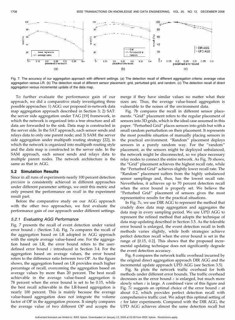
Fig. 7 presents the recall of event detection under variederror bound " (Section 3.4). Fig. 7a compares the recall ofthe aggregation based on LR adopted in AGG approachwith the simple average value-based one. For the aggrega-tion based on LR, the error bound refers to the user-defined error bound " introduced in Section 3.4. For theaggregation based on average values, the error boundrefers to the difference ratio between two OP. As the figureshows, the aggregation based on LR provides much higherpercentage of recall, overcoming the aggregation based onaverage values by more than 20 percent. The best recallachievable in the average value-based aggregation is78 percent when the error bound is set to be 0.15, whilethe best recall achievable in the LR-based aggregation isnearly 100 percent. This is mainly because the averagevalue-based aggregation does not integrate the volumefactor of OP in the aggregation process. It simply comparesthe average value of two different OP and accepts the

merge if they have similar values no matter what theirsizes are. Thus, the average value-based aggregation isvulnerable to the noises of the environment data.

Fig. 7b compares the recall in different sensor place-ments. “Grid” placement refers to the regular placement ofsensors into 3D grids, which is the ideal case assumed in thispaper. “Perturbed Grid” places sensors into grids but with asmall random perturbation on their placement. It representsthe most possible situation of manually placing sensors inthe practical environment. “Random” placement deployssensors in a purely random way. For the “random”placement, as the sensors might be deployed unbalanced,the network might be disconnected, so we place necessaryrelay nodes to connect the entire network. As Fig. 7b shows,the “Grid” placement achieves the highest recall rate, whilethe “Perturbed Grid” achieves slightly lower recall rate. The“Random” placement suffers from the highly unbalancedsensor samplings and, thus, has the lowest recall rate.Nevertheless, it achieves up to 70 percent detection recallwhen the error bound is properly set. We believe the“Perturbed Grid” placement of sensors gives the mostrepresentative results for the practical situations.

In Fig. 7c, we use DIR AGG to represent the method thatcrudely does data map aggregation and aggregates thedata map in every sampling period. We use UPD AGG torepresent the refined method that adopts the technique ofdata map updating described in Section 3.5. As the tolerableerror bound is enlarged, the event detection recall in bothmethods varies slightly, while both strategies achieveperfect detection recall when the error bound is set in therange of [0.15, 0.2]. This shows that the proposed incre-mental updating technique does not significantly degradethe event detection accuracy.

Fig. 8 compares the network traffic overhead incurred bythe original direct aggregation approach DIR AGG and theincremental update approach UPD AGG (see Section 3.5).

Fig. 8a plots the network traffic overhead for bothmethods under different error bounds. The traffic overheaddecreases as the error bound " is enlarged, but much moreslowly when " is large. A combined view of this figure andFig. 7c suggests an optimal choice of the error bound " atabout 0.2, which provides perfect detection recall withcomprehensive traffic cost. We adopt this optimal setting of" for later experiments. Compared with the DIR AGG, theUPD AGG achieves almost the same detection recall but


Fig. 7. The accuracy of our aggregation approach with different settings. (a) The detection recall of different aggregation criteria: average value

aggregation versus LR. (b) The detection recall of different sensor placement: grid, perturbed grid, and random. (c) The detection recall of direct

aggregation versus incremental update of the data map.


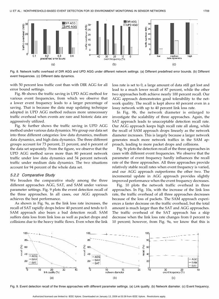
with 50 percent less traffic cost than with DIR AGG for allerror bound settings.

Fig. 8b shows the traffic saving in UPD AGG method forvarious event frequencies, from which we observe thata lower event frequency leads to a larger percentage ofsaving. That is because the data map updating techniqueadopted in UPD AGG method reduces more unnecessarytraffic overhead when events are rare and historic data areaggressively utilized.

Fig. 8c further shows the traffic saving in UPD AGGmethod under various data dynamics. We group our data setinto three different categories: low data dynamics, mediumdata dynamics, and high data dynamics. The three differentgroups account for 73 percent, 21 percent, and 6 percent ofthe data set separately. From the figure, we observe that theUPD AGG method saves more than 80 percent networktraffic under low data dynamics and 54 percent networktraffic under medium data dynamics. The two situationsaccount for 94 percent of the whole data set.

5.2.2 Comparative Study

We broaden the comparative study among the threedifferent approaches AGG, SAT, and SAM under variousparameter settings. Fig. 9 plots the event detection recall ofthe three approaches. In all cases, our AGG approachachieves the best performance.

As shown in Fig. 9a, as the link loss rate increases, therecall of SAT rapidly drops below 40 percent and tends to 0.SAM approach also bears a bad detection recall. SAMsuffers data loss from link loss as well as packet drops andcollisions due to the heavy traffic flows. Even when the link

loss rate is set to 0, a large amount of data still get lost andlead to a much lower recall of 87 percent, while the othertwo approaches both achieve nearly 100 percent recall. OurAGG approach demonstrates good tolerability to the net-work quality. The recall is kept above 60 percent even in alossy network with up to 40 percent link loss rate.

In Fig. 9b, the network diameter is enlarged toinvestigate the scalability of three approaches. Again, theSAT approach leads to unacceptable detection recall rate.Our AGG approach keeps high recall rate all along, whilethe recall of SAM approach drops linearly as the networkdiameter increases. This is largely because a larger networkgenerates much more network traffics in the SAM ap-proach, leading to more packet drops and collisions.

Fig. 9c plots the detection recall of the three approaches incases with different event frequencies. We observe that theparameter of event frequency hardly influences the recallrate of the three approaches. All three approaches providerelatively stable recall rates when event frequency is varied,and our AGG approach outperforms the other two. Theincremental update in AGG approach provides slightlyimproved performance when the event frequency decreases.

Fig. 10 plots the network traffic overhead in threeapproaches. In Fig. 10a, with the increase of the link lossrate, the traffic overhead of all three approaches decreasesbecause of the loss of packets. The SAM approach experi-ences a faster decrease on the traffic overhead, but the totalamount is much larger than the SAT and AGG approaches.The traffic overhead of the SAT approach has a skipdecrease when the link loss rate changes from 0 percent to10 percent; however, from Fig. 9a, we know that this is


Fig. 8. Network traffic overhead of DIR AGG and UPD AGG under different network settings. (a) Different predefined error bounds. (b) Different

event frequencies. (c) Different data dynamics.

Fig. 9. Event detection recall of the three approaches with different parameter settings. (a) Link quality. (b) Network diameter. (c) Event frequency.


because most of the useful information gets lost due to thepacket loss. Thus, although SAT has the lowest trafficoverhead, it provides nearly unacceptable event detectionrecall. Fig. 10b shows how network traffic overhead growsas the network size increases. We note that while the SATand AGG approaches maintain comparatively low trafficoverhead against the increase of network diameter, the SAMapproach has a dramatic increase of traffic overhead, whichgreatly constrains its scalability. Fig. 10c shows how theparameter of event frequency affects the three approaches.While the event frequency has little influence on SAM andSAT approaches, the traffic overhead of our AGG approachis reduced as the event frequency decreases, benefiting fromthe data map updating technique. According to our fieldinvestigation in the coal mine, generally, the event fre-quency in the real world remains low, benefiting theapplication of our AGG approach.

To summarize, among the three possible approaches, theSAT approach introduces the least traffic overhead butprovides the worst, totally unacceptable event detectionaccuracy; the SAM approach provides somewhat tolerableevent detection accuracy but with the most traffic overheadand the worst scalability; our AGG approach provides thebest event detection performance with relatively smalltraffic overhead. We also achieve the best scalability to thenetwork size and tolerability to the network quality in theAGG approach.

6 CONCLUSIONS AND FUTURE WORK

In this paper, we have proposed a nonthreshold-basedapproach for complex event detection in 3D environmentmonitoring applications. Other than threshold-based ap-proaches, we have proposed event feature patterns tospecify complex events and developed a pattern-basedevent detection method on the obtained 3D gradient datamap. We employ multipath routing architectures to providerobust data delivery and perform in-network aggregationon it to efficiently construct the data map. Space OP modelis proposed to describe the environment data distributions.Partial data maps are aggregated by merging OP regionswith similar environmental data. The incremental updatefor the gradient data map explores the usability of historicdata while the environment is stable with low frequency ofevents and further reduces unnecessary data delivery. Ourexperimental results show the performance gain of our

energy-efficient techniques. Moreover, the comparativestudy with two alternative approaches exhibits that ourapproach achieves great event detection accuracy withsmall network traffic overhead.

The future work includes implementing a workingsystem in real-world environment. To carry on, patternrecognition on the obtained gradient data maps withmachine learning techniques on historic data samples mayprovide more efficient detection methods, which will alsobe included in our future work.

ACKNOWLEDGMENTS

This work was supported in part by the Hong KongRGC Grants HKUST6169/07E and HKUST 6119/07E, bythe National High Technology Research and Develop-ment Program of China (863 Program) under Grant2007AA01Z180, by the National Basic Research Programof China (973 Program) under Grant 2006CB303000, bythe HKUST Nansha Research Fund NRC06/07.EG01, andby the NSFC Key Project Grants 60533110, 60736016, and60736013.

REFERENCES

[1] A. Aguilera and D. Ayala, “Orthogonal Polyhedra as GeometricBounds in Constructive Solid Geometry,” Proc. Solid and PhysicalModeling Symp. (SPM), 1997.

[2] R. Baeza-Yates and R.N. Berthier, Modern Information Retrieval.Addison-Wesley, 1999.

[3] P. Bonnet, J. Gehrke, and P. Seshadri, “Querying the PhysicalWorld,” IEEE Personal Comm., vol. 7, 2000.

[4] R. Burns, A. Terzis, and M. Franklin, “Design Tools for Sensor-Based Science,” Proc. Third Workshop Embedded Networked Sensors(EmNets), 2006.

[5] A. Chakrabarti, A. Sabharwal, and B. Aazhang, “Using Predict-able Mobility for Power Reduction in Sensor Networks,” Proc.Second IEEE/ACM Int’l Workshop Information Processing in SensorNetworks (IPSN), 2003.

[6] W. Choi, P. Shah, and S.K. Das, “A Framework for Energy-SavingData Gathering Using Two-Phase Clustering in Wireless SensorNetworks,” Proc. First IEEE Ann. Int’l Conf. Mobile and UbiquitousSystems (MobiQuitous), 2004.

[7] J. Considine, F. Li, G. Kollios, and J. Byers, “ApproximateAggregation Techniques for Sensor Databases,” Proc. 20th IEEEInt’l Conf. Data Eng. (ICDE), 2004.

[8] D. Donjerkovic, Y. Loannidis, and R. Ramakrishnan, “DynamicHistograms: Capturing Evolving Data Sets,” Proc. 16th IEEE Int’lConf. Data Eng. (ICDE), 2000.

[9] P. Dutta, M. Grimmer, A. Arora, S. Bibyk, and D. Culler, “Designof a Wireless Sensor Network Platform for Detecting Rare,Random, and Ephemeral Events,” Proc. Fourth IEEE/ACM Int’lSymp. Information Processing in Sensor Networks (IPSN), 2005.


Fig. 10. Network traffic overhead of the three approaches with different parameter settings. (a) Link quality. (b) Network diameter. (c) Event

frequency.


[10] F. Furfaro, G.M. Mazzeo, and C. Sriangelo, “Exploiting ClusterAnalysis for Constructing Multi-Dimensional Histograms on BothStatic and Evolving Data,” Proc. 10th Int’l Conf. Extending DatabaseTechnology (EDBT), 2006.

[11] W.R. Heinzelman, A. Chandrakasan, and H. Balakrishnan,“Energy-Efficient Communication Protocol for Wireless Micro-sensor Networks,” Proc. 33rd Hawaii Int’l Conf. System Sciences(HICSS), 2000.

[12] J.M. Hellerstein, W. Hong, S. Madden, and K. Stanek, “BeyondAverage: Toward Sophisticated Sensing with Queries,” Proc.Second IEEE/ACM Int’l Workshop Information Processing in SensorNetworks (IPSN), 2003.

[13] J. Hill and D. Culler, “Mica: A Wireless Platform for DeeplyEmbedded Networks,” IEEE Micro, vol. 22, pp. 12-24, 2002.

[14] C. Intanagonwiwat, R. Govindan, and D. Estrin, “DirectedDiffusion: A Scalable and Robust Communication Paradigm forSensor Networks,” Proc. ACM MobiCom, 2000.

[15] M. Li and Y. Liu, “Underground Structure Monitoring withWireless Sensor Networks,” Proc. Sixth IEEE/ACM Int’l Symp.Information Processing in Sensor Networks (IPSN), 2007.

[16] S. Li, Y. Lin, S. Son, J. Stankovic, and Y. Wei, “Event DetectionServices Using Data Service Middleware in Distributed SensorNetworks,” Telecomm. Systems J., vol. 26, 2004.

[17] Z. Li and B. Li, “Loss Inference in Wireless Sensor NetworksBased on Data Aggregation,” Proc. Third IEEE/ACM Int’l Symp.Information Processing in Sensor Networks (IPSN), 2004.

[18] S. Lindsey, C. Raghavendra, and K. Sivalingam, “Data Gatheringin Sensor Networks Using Energy Delay Metric,” Proc. IPDPSWorkshops, 2001.

[19] S. Madden, M.J. Franklin, and J.M. Hellerstein, “TAG: A TinyAggregation Service for Ad-Hoc Sensor Networks,” Proc. FifthSymp. Operating System Design and Implementation (OSDI), 2002.

[20] X. Meng, T. Nandagopal, L. Li, and S. Lu, “Contour Maps:Monitoring and Diagnosis in Sensor Networks,” Computer Net-works, 2006.

[21] V. Mhatre, C. Rosenberg, D. Kofman, R. Mazumdar, andN.B. Shroff, “Design of Surveillance Sensor Grids with aLifetime Constraint,” Proc. First European Workshop WirelessSensor Networks (EWSN), 2004.

[22] S. Nath, P.B. Gibbons, S. Seshan, and Z.R. Anderson, “SynopsisDiffusion for Robust Aggregation in Sensor Networks,” Proc. SecondACM Conf. Embedded Networked Sensor Systems (SenSys), 2004.

[23] S.-J. Park, R. Vedantham, R. Sivakumar, and I.F. Akyildiz, “AScalable Approach for Reliable Downstream Data Delivery inWireless Sensor Networks,” Proc. ACM MobiHoc, 2004.

[24] I. Solis and K. Obraczka, “Efficient Continuous Mapping in SensorNetworks Using Isolines,” Proc. Second IEEE Ann. Int’l Conf. Mobileand Ubiquitous Systems (MobiQuitous), 2005.

[25] Y. Tian, E. Ekici, and F. Ozguner, “Energy-Constrained TaskMapping and Scheduling in Wireless Sensor Networks,” Proc.Workshop Resource Provisioning and Management in Sensor Networks(RPMSN), 2005.

[26] N. Xu et al., “A Wireless Sensor Network for StructuralMonitoring,” Proc. Second ACM Conf. Embedded NetworkedSensor Systems (SenSys), 2004.

[27] M. Younis, P. Munshi, and E. Al-Shaer, “Architecture for EfficientMonitoring and Management of Sensor Networks,” Proc. SixthIFIP/IEEE Int’l Conf. Management of Multimedia Networks andServices (MMNS), 2003.

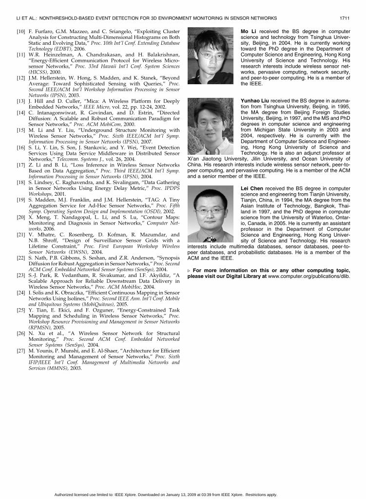
Mo Li received the BS degree in computerscience and technology from Tsinghua Univer-sity, Beijing, in 2004. He is currently workingtoward the PhD degree in the Department ofComputer Science and Engineering, Hong KongUniversity of Science and Technology. Hisresearch interests include wireless sensor net-works, pervasive computing, network security,and peer-to-peer computing. He is a member ofthe IEEE.

Yunhao Liu received the BS degree in automa-tion from Tsinghua University, Beijing, in 1995,the MA degree from Beijing Foreign StudiesUniversity, Beijing, in 1997, and the MS and PhDdegrees in computer science and engineeringfrom Michigan State University in 2003 and2004, respectively. He is currently with theDepartment of Computer Science and Engineer-ing, Hong Kong University of Science andTechnology. He is also an adjunct professor at

Xi’an Jiaotong University, Jilin University, and Ocean University ofChina. His research interests include wireless sensor network, peer-to-peer computing, and pervasive computing. He is a member of the ACMand a senior member of the IEEE.

Lei Chen received the BS degree in computerscience and engineering from Tianjin University,Tianjin, China, in 1994, the MA degree from theAsian Institute of Technology, Bangkok, Thai-land in 1997, and the PhD degree in computerscience from the University of Waterloo, Ontar-io, Canada, in 2005. He is currently an assistantprofessor in the Department of ComputerScience and Engineering, Hong Kong Univer-sity of Science and Technology. His research

interests include multimedia databases, sensor databases, peer-to-peer databases, and probabilistic databases. He is a member of theACM and the IEEE.

. For more information on this or any other computing topic,please visit our Digital Library at www.computer.org/publications/dlib.



Documents

IEEE TRANSACTIONS ON KNOWLEDGE AND DATA … · We employ energy-efficient ... query processing, wireless sensor networks. ... more reliable message delivery in the lossy sensor network