IEEE TRANSACTIONS ON INTELLIGENT …hbling/publication/TITS_04092017-L.pdf · A Dense Correspondence based Transfer Learning Approach Shuai Di, Honggang Zhang, Senior Member, IEEE,

IEEE TRANSACTIONS ON INTELLIGENT TRANSPORTATION SYSTEMS, VOL. XX, NO. XX, XXX 20XX 1

Cross-domain Traffic Scene Understanding:A Dense Correspondence based Transfer Learning

ApproachShuai Di, Honggang Zhang, Senior Member, IEEE, Chun-Guang Li Member, IEEE, Xue Mei, Senior

Member, IEEE, Danil Prokhorov, Senior Member, IEEE, and Haibin Ling

Abstract—Understanding traffic scene images taken fromvehicle-mounted cameras is important for high level tasks such asAdvanced Driver Assistance Systems (ADASs) and autonomousdriving. It is a challenging problem due to large variations underdifferent weather or illumination conditions. In this paper, wetackle the problem of traffic scene understanding from a cross-domain perspective. Specifically, we attempt to understand thetraffic scene from images taken from the same location but underdifferent weather or illumination conditions (e.g. understandingthe same traffic scene from images on a rainy night with the helpof images taken on a sunny day). To this end, we propose a DenseCorrespondence based Transfer Learning (DCTL) approach,which consists of three main steps: a) extracting deep representa-tions of traffic scene images via a Convolutional Neural Network(CNN), b) constructing compact and effective representationsvia cross-domain metric learning and subspace alignment forcross-domain retrieval, and c) transferring the annotations fromthe retrieved best matching image to the test image based oncross-domain dense correspondences and a probabilistic Markovrandom field (MRF). To verify the effectiveness of our DCTLapproach, we conduct extensive experiments on a challengingdata set, which contains 1,828 images from six weather orillumination conditions.

Index Terms—Traffic scene understanding, semantic segmenta-tion, transfer learning, dense correspondence, road scene, vehicleenvironment perception.

I. INTRODUCTION

Understanding traffic scenes from images taken by vehicle-mounted cameras is important for situational awareness inIntelligent Transportation System (ITS), such as AdvancedDriver Assistance Systems (ADAS) and autonomous driving.The state of art has mainly focused on road related detections,such as road layout detection [1], [2] and road markingdetection [3], [4], [5], [6]. It is well accepted that a practicalautonomous driving system requires reliable and effective traf-fic scene understanding [7], [8], [9], [10]. Existing approaches

S. Di is with the School of Information and Communication Engineering,Beijing University of Posts and Telecommunications, Beijing 100876, China(e-mail: [email protected]).

H. Zhang and C.-G. Li are with the School of Information and Commu-nication Engineering, Beijing University of Posts and Telecommunications,Beijing 100876, China (e-mail: {zhhg, lichunguang}@bupt.edu.cn).

X. Mei and D. Prokhorov are with the Toyota Research Institute, NorthAmerica, Ann Arbor, MI 48105 USA (e-mail: [email protected];[email protected]).

H. Ling is with the Department of Computer and InformationSciences, Temple University, Philadelphia, PA 19122 USA (e-mail:[email protected]). Corresponding author.

Manuscript received XXX, XX, 20XX; revised XXX, XX, 20XX.

in traffic scene understanding, however, are sensitive to thelarge variations due to weather or illumination changes.

In this paper, we address the problem from a cross-domaintransfer learning perspective, i.e. addressing it by using imagesof the same location but taken in other weather or illuminationconditions. We assume that the annotated training imagesunder good weather or illumination conditions are availablefor our reference. We view different weather or illuminationconditions as different domains. Therefore, our problem iseffectively a cross-domain learning problem.

Our basic idea is to find a subset of well-annotated images ingood weather or illumination conditions and then transfer theirannotations to the test image. Specifically, we propose a DenseCorrespondence based Transfer Learning (DCTL) approach,in which we construct compact representations for finding thebest matching image in a training set across domains, andthen infer the annotations of the test image by building cross-domain dense correspondences between the test image and theretrieved best matching image in the training set.

In our proposed DCTL approach, we fine-tune a pre-trained Convolutional Neural Network (CNN) to extract deeprepresentations of traffic scene images at first, and then per-form domain adaptation to construct compact and effectiverepresentations for retrieving the best matching image in thetraining set across different domains (i.e. weather or illumina-tion conditions). Finally, cross-domain dense correspondencesbetween the test image and the best matching image withannotations are built via SIFT flow, and the annotations fromthe training images are transferred to the test image viaa probabilistic MRF model. We verify effectiveness of ourproposed approach on a challenging data set.

We summarize contributions of our paper below:• We propose a dense correspondence based transfer learn-

ing framework for understanding traffic scene imagesunder challenging variations of weather or illuminationconditions. To the best of our knowledge, this is the firsttime that the traffic scene understanding is approached bytransferring information from images of the same locationtaken in different conditions.

• We evaluate performance of state-of-the-art CNNs withdifferent architectures, pre-trained on different data sets,with their deep features extracted from different layers.

• We collect samples to build a challenging image dataset, which contains 1,828 images from six weather orillumination conditions. This data set is available online


for free to use for ITS research.The remainder of this paper is arranged as follows. In

Section II, we review the related work. In Section III, wepresent our DCTL approach. In Section IV, we describe ourextensive experiments, followed by our conclusions in SectionV.

II. RELATED WORKS

Our cross-domain transfer learning approach for trafficscene understanding is related to place recognition, domainadaptation, and scene recognition and semantic segmentationwith deep learning.

A. Place Recognition

In the past few years, place recognition has achieved greatprogress [11], [12], [13], [14], [15], [16]. Roughly, the taskof place recognition is treated as a variant of image retrievalproblem [17]. The state-of-the-art approaches for place recog-nition are based on local invariant features, including image-level descriptors [16], [12] or reconstructed 3D points [15],[14]. In [13], Milford et al. introduce a condition-invariantmethod for place recognition, in which the images of thesame location are matched and the highly aliased images fromdifferent locations are rejected. However, there is a lack ofmethods for understanding traffic scene images under differentweather or illumination conditions.

B. Subspace-based Domain Adaptation

The idea of subspace-based domain adaptation is to projectboth source data and target data into a common subspace tomake the distributions of the two sources as consistent aspossible [18], [19], [20], [21]. We assume that there are manylabeled data in the source domain but few in the target domain.We aim at adapting information from the labeled data in thesource domain to the new data in the target domain.

In traffic scene understanding, we view the weather orillumination conditions as domains, and we treat our problemas cross-domain learning. We address the problem of recog-nizing images of the same scene across domains by learninga transform utilizing the data from two domains, and thedomains may have large appearance variations.

C. Deep Learning for Scene Recognition/Semantic Segmenta-tion

CNN based models have been the top performers on scenerecognition tasks [22], [23], [24], [25]. In recent works [26],[27], [28], [29], deep CNN features learned on large data sets,such as ImageNet (ILSVRC) [30] and Places [23], [31], canbe used as powerful descriptors to other applications.

However, traffic scene images considered in this paper havesignificant appearance variations. This differs from imagesin other data sets, such as those used for training ImageNet(ILSVRC) and Places which might not adequate for dealingwith traffic scene images.

Deep architectures designed for semantic scene segmenta-tion have also achieved the state-of-the-art results by learning

TABLE IPAIR-WISE DOMAINS FOR THE CROSS-DOMAIN TRAFFIC SCENE DATASET.

High contrast domains:sunny day−→ night sunny day−→ rainy nightcloudy day−→ night cloudy day−→ rainy nightsnowy day−→ night snowy day−→ rainy night

Low contrast domains:sunny day−→ foggy day sunny day−→ snowy day

cloudy day−→ snowy day rainy night−→ night

to decode low resolution image representations to pixel-wisepredictions such as [32], [33], [34], [35], [36]. The perfor-mance of these methods may degenerate if the images havelarge appearance variations as in our problem. Different fromtraining a deep network directly, we perform our semanticscene segmentation by building dense correspondences be-tween a test image and annotated images of the training set.

III. OUR PROPOSAL: DENSE CORRESPONDENCE BASEDTRANSFER LEARNING APPROACH

We describe our problem setting, followed by our proposedapproach.

Problem Settings: We consider the following six typicalweather and illumination conditions: sunny day, night, snowyday, rainy night, cloudy day and foggy day, with each con-dition viewed as a specific domain. Each domain containstraffic scene images taken at different locations, and eachlocation is selected as one class. In addition, pair-wise domainsare assembled and divided into two groups in terms of theirillumination contrast: low contrast domains and high contrastdomains as shown in Table I. The symbol “−→” in the tablepoints from the source domain to the target domain, and itmeans that we want to understand the traffic scene images inthe target domain by transferring information from images inthe source domain. We also select very challenging scenarios,e.g. night and rainy night as the target domains, with otherscenarios as the source domains.

We illustrate the flowchart of our proposed approach DCTLin Fig. 1. The approach consists of three stages:• Extracting deep features via a fine-tuned CNN;• Constructing compact and effective representations via

cross-domain metric learning and subspace alignment forcross-domain retrieval;

• Building cross-domain dense correspondences for trans-ferring annotations.

A. Extracting Deep Representation

As shown in [26], [27], [28], [29], [37], a well-trained CNNcan be used to generate powerful descriptors for applicationson diverse data sets. Different CNN architectures have beenproposed recently, e.g. VGG [28], [24], GoogLeNet [25], andDeCAF [26], [38]. We compare performance of their deeprepresentations on traffic scene images.

As shown in [38], [28], fine-tuning the pre-trained CNN ona specific data set can improve the performance significantly.In our case, image appearances from our traffic scene data


Fig. 1. Flowchart of the cross-domain traffic scene understanding.

sets are quite different from those in data sets used to pre-train CNN. That is why we fine-tune the pre-trained CNN onour traffic scene data sets.

A CNN often contains a huge number of adjustable pa-rameters, e.g. more than 60 million parameters in the CNNarchitecture from [22]. Learning effectively so many param-eters using images from modest-size data sets is infeasible.As shown in [26], [27], [39], the internal layers of theCNN can act as a generic extractor of image representations.Parameters of the internal layers of the pre-trained networkscan remain unchanged before fine-tuning. In addition, dataaugmentation is applied, which is used to enlarge the data setartificially using label-preserving transformations [22], [27].More specifically, we combine the horizonal reflections withcrops, which is similar to recent data augmentation methodsfor training CNN [22], [27], [28]. In our data augmentation,ten samples are produced for each original image.

B. Domain Adaptation and Subspace AlignmentTraffic scene images taken in different weather or illumina-

tion conditions may have dramatic appearance variations, andthe extracted deep features may also be exhibiting large featurevariations. We tackle this difficulty by domain adaptation. Aslisted in Table I, the condition on the left side of the arrowis domain A and the condition on the right side of the arrowis domain B. For example, “sunny day”, “cloudy day”, and“snowy day” are domain A; whereas “night”, “rainy night”,and “foggy day” are domain B.

Our idea is to transfer the annotation information of trafficscene images in domain A to the test image in domain B. Todo so, we need to find in the training set of domain A a subsetof images, which are the best match to the test image. We thentransfer the annotations by building dense correspondences tobe described in the next subsection.

1) Training Stage: PLS Regression and Cross-Domain Met-ric Learning: Generally, PCA is the most popular method forlinear dimension reduction before conducting metric learning.However, PCA is not able to preserve the latent structureacross different domains as in our case. Therefore, instead,we apply PLS regression [40] on data from the two domainsto learn compact representations of a common subspace.

Let training data in domain A and domain B be X(a) =

[x(a)1 , . . . , x(a)

n ] and X(b) = [x(b)1 , . . . , x(b)

m ], which contain nand m deep features of d-dimension, respectively. Moreover,we arrange the labels of the training samples in domain A

and domain B into label matrices Y (a) = [y(a)1 , . . . , y

(a)n ]

and Y (b) = [y(b)1 , . . . , y

(b)m ], respectively, in which the labels

y(a)i and y(b)

j indicate the specific locations where the trainingsamples are taken. If y(a)

i = y(b)j , we call the paired samples

(x(a)i , x(b)

j ) as a positive sample pair, otherwise we call it as anegative sample pair.

PLS regression is applied to the training data {X(a), X(b)},to obtain the projection matrix P of d×p, where p < d is thetarget dimension.

We denote the PLS dimension-reduced data as X̃(a) andX̃(b), where X̃(a) = PTX(a) and X̃(b) = PTX(b). Then, welearn a metric to measure the cross-domain distance betweendata samples from the two domains:

‖x̃(a) − x̃(b))‖2W = (x̃(a) − x̃(b))TW (x̃(a) − x̃(b)), (1)

where W is a positive semi-definite matrix of p× p.Let W = V V T in which V ∈ Rp×q with q < p, we have

that:

‖x̃(a) − x̃(b))‖2W = ‖V T x̃(a) − V T x̃(b)‖22, (2)

Similar to [41], we use the log-logistic loss function asfollows:

`W (x̃(a)i , x̃(b)

j ) = log(1 + eθij(‖x̃(a)i −x̃(b)j ‖

2W−c)), (3)

where θij = 1 if y(a)i = y

(b)j and otherwise θij = −1, c is a

constant. Then, by using W = V V T , our cross-domain metriclearning problem is formulated as follows:

minV

n∑i=1

m∑j=1

αij`V V T (x̃(a)i , x̃(b)

j ), (4)

where αij = 1N+

if θij = 1 and 1N−

otherwise, and N+ andN− are the numbers of positive and negative sample pairs,respectively. Note that the weighting scheme is importantbecause N+ and N− are heavily unbalanced in our problem.


We solve problem (4) by the accelerated proximal gradientoptimization method as in [41]. After the optimization processcompletion, we obtain the optimal solution V∗ and apply it tofind a compact and effective representation of the test data.

2) Testing Stage: Subspace Alignment: In the training stage,we perform PLS regression and cross-domain metric learningon the training data to minimize the discrepancy in the twodomains. We obtain a latent structure preserving projectionmatrix P and a supervised domain adaptation projectionmatrix V∗.

In the testing stage, we apply the cross-domain projectionsP and V∗ to reduce the dimensionality of the test data asfollows:

Z̃(a) = V T∗ PTZ(a), (5)

Z̃(b) = V T∗ PTZ(b), (6)

where Z(a) = [z(a)1 , . . . , z(a)

s ] and Z(b) = [z(b)1 , . . . , z(b)

t ]contain s and t testing samples of d-dimension in domain Aand domain B, respectively.

To further minimize the discrepancy between the two do-mains, we align subspace Z̃(a) in domain A with respectto subspace Z̃(b) in domain B. Let Q(a) ∈ Rq×k andQ(b) ∈ Rq×k be the left singular matrices of Z̃(a) and Z̃(b),respectively, then we can find an alignment matrix R byminimizing the Bregman matrix divergence [18] as follows:

minR‖Q(a)R−Q(b)‖2F , (7)

where ‖ · ‖F is the Frobenius norm. Note that the closed-form solution is R∗ = QT(a)Q(b). Then, Z̃(a) and Z̃(b) can beprojected into a common subspace as follows:

C(a) = RT∗QT(a)Z̃

(a), (8)

C(b) = RT∗QT(b)Z̃

(b), (9)

where C(a) ∈ Rk×s and C(b) ∈ Rk×t are the compact cross-domain representations for test data in domain A and domainB, respectively. For each test sample in domain B, we use itsk-dimensional representation to find the best matching samplesin domain A.

Remark. In [42], a metric learning is used to generatesubspaces of the source domain. Unlike [42], we learn a metricon the cross-domain training data (resp. just one scenario data)and transfer the data which are different to the data used forlearning the metric (resp. the same data used for learning themetric) into the metric-induced space.

C. Scene Understanding through Label Transfer

While the images in different domains are usually of dif-ferent appearances due to variations from weather or illumi-nation conditions, they share similar spatial layout structure.Therefore, the annotation information on scene images indomain A can be transferred into scene images in domain Bif correct correspondences are properly created. In this paper,we build the dense correspondences via SIFT flow [43], [44]and transfer the annotation information via a Markov randomfield model.

1) Cross-domain Dense Correspondence via SIFT Flow:The goal of SIFT flow is to find the dense correspondencesbetween two images. We consider a test image, denoted asI(b) and the best matching image, denoted as I(a). Let p bethe spatial coordinates of a pixel in the image, and f(b)(p) bethe SIFT descriptor [45] at coordinates p in the test imageI(b), f(a)(p) be the SIFT descriptor at coordinates p in thebest matching image I(a), and w(p) be the displacement ofthe corresponding SIFT feature in image I(a). Similar to [46],we define the energy function of SIFT flow field1 W on thebest matching image I(a) with respect to test image I(b) asfollows:

ε(W) =∑p

‖f(b)(p)− f(a)(p+ w(p))‖2

+ λ∑

(p,q)∈E

‖w(p)− w(q)‖22,(10)

where E contains all of the spatial neighborhood (4-neighborgraph) and λ is the regularization parameter. We solve forW by minimizing the energy function ε(W) using beliefpropagation [47].

2) Annotation Transfer: Given a test image I(b) with itscorresponding SIFT descriptor field 2 F(I(b)), the best match-ing image I(a) with its corresponding SIFT descriptor fieldF(I(a)) and annotation field3 L(I(a)), and the SIFT flowfield W∗ obtained from solving (10), our goal is to infer theannotation defined for each pixel in I(b), i.e. the annotationfield L(I(b)) for test image I(b).

To infer the annotation field L(I(b)), we consider the densecorrespondences between I(b) and I(a), spatial layout priorinformation on I(b) and the spatial smoothness in I(b).

To utilize the dense correspondences established by SIFTflow similar to [48], we define a penalty term φ(L(I(b), p))as:• If L(I(b), p) = L(I(b), p+ w∗(p)), then

φ(L(I(b), p)) = ‖f(b)(p)− f(a)(p+ w∗(p))‖2. (11)

• If L(I(b), p) 6= L(I(b), p+ w∗(p)), then

φ(L(I(b), p)) = χ, (12)

where L(I(b), p) is the annotation at position p inimage I(b), and χ is sufficiently large, e.g. χ =maxp,q ‖f(b)(p)− f(a)(q)‖2.

To utilize our spatial prior, we define the penalty term:

θ(L(I(b), p)) = − logH(p), (13)

where H(p) denotes the prior probability of pixel p to belongto an object category, and it can be estimated by calculatingthe spatial histogram of the object category for each pixel inthe training set. We show examples of estimated H in ourcross-domain traffic scene data sets in Fig. 2.

To take into account smoothness, we define penalty termψ(L(I(b), p),L(I(b), q)) for assigning labels L(I(b), p) andL(I(b), q) to two adjacent pixels below:

1A set of displacements w(p) defined on the whole image.2A set of SIFT descriptors is defined on the whole image.3A set of annotated labels is defined on the whole image indicating the

category of object at pixel p.


building bridge

car median strip

pole road

sky traffic lights

traffic sign tree

Fig. 2. The statistics for spatial priors of some object categories in ourcross-domain traffic scene data set. Note that white means the probabilityof appearance for this category is zero. The denser the color, the higher theprobability.

• If L(I(b), p) 6= L(I(b), q), then

ψ(L(I(b), p),L(I(b), q)) = e−γ‖I(b)(p)−I(b)(q)‖22 , (14)

where γ is an image-dependent contrast constant4.• If L(I(b), p) = L(I(b), q), then

ψ(L(I(b), p),L(I(b), q)) = 0. (15)

To accurately infer the annotaion field L(I(b)), similarto [44], we build a probabilistic MRF model by integratingdense correspondences, spatial prior information and spatialsmoothness as follows:

minL(I(b))

∑p

φ(L(I(b), p)) + α∑p

θ(L(I(b), p))

+β∑

(p,q)∈E

ψ(L(I(b), p),L(I(b), q)).(16)

Finally, we solve for L(I(b)) by using the belief propagationalgorithm.

Remark. Our task of traffic scene understanding involvessemantic labeling or segmentation only. In general, trafficscene understanding should also infer the spatial relationshipof the recognized objects. This may be a subject of futureresearch.

IV. EXPERIMENTS

To validate effectiveness of our proposed approach, weconduct our extensive experimental evaluation.

4The γ ensures that the exponential term in (14) switches properly betweenhigh and low contrasts [49]. Usually, γ = 0.5

E[‖I(b)(p)−I(b)(q)‖2], E[·] is the

expectation taken over image I(b).

sunny day (city) sunny day (highway)

night (city) night (highway)

snowy day (city) snowy day (highway)

rainy night (city) rainy night (highway)

cloudy day (city) cloudy day (highway)

Location I Location II

Fig. 3. Example images from our cross-domain traffic scene data set (firstroute). Images for two different locations are shown. Each location containstraffic scene images varying from weather and illumination (top to bottom).

A. Data Set and Evaluation Metric

1) Data Set: Our cross-domain traffic scene data set con-sists of traffic scene images collected from two road routes.The images of the first road route are from five video se-quences captured by our test vehicle. It consists of 1,130traffic scene images of 226 different locations. Both trafficscenes for city and highway are included in this road route. Allvideos were captured on the same road route, but with differentweather and illumination conditions. At each location, wecaptured images of 5 different conditions, i.e. “sunny day”,“night”, “snowy day”, “rainy night” and “cloudy day”, asillustrated in Fig. 3. All of the images are of 856×270 pixels.

The images of the second road route are from two video se-quences collected from YouTube. Specifically, the image dataconsists of 698 traffic scene images of 349 different locations.At each location, 2 different conditions were captured, i.e.“sunny day” and “foggy day”, as illustrated in Fig. 4. All ofthe images are of 640×360 pixels.

In addition, all of the 1,130 images collected from the firstroute, and 100 images (50 pair-wise images) collected fromthe second route are manually annotated with LabelMe [50].There are 13 object categories for the annotated images. Anyother object categories are classified as undefined category.The statistics of the annotated object categories are shown inFig. 5 and Fig. 6. This data set is available online for free touse for research purpose. 5

2) Evaluation Metrics: To evaluate different deep represen-tations and cross-domain approaches, we calculate CumulativeMatching Characteristic (CMC) curve, which is commonlyused as a measure of identification system [41], [51]. Our

5www.dabi.temple.edu/∼hbling/data/scene-itsc16/benchmark itsc16.html.

www.dabi.temple.edu/~hbling/data/scene-itsc16/benchmark_itsc16.html


0

0.1

0.2

0.3

0.4

0.5

0.6

sky building

tree undefined

roadcar median strip

bridgevegetation

traffic sign

poletraffic lights

pedestrian

0

0.1

0.2

0.3

0.4

0.5

0.6

sky undefined

building


bridgetree traffic sign

polevegetation

traffic lights

pedestrian

0

0.1

0.2

0.3

0.4

0.5

0.6

sky building

undefined

tree roadcar median strip

bridgetraffic sign

polevegetation

traffic lights

0

0.1

0.2

0.3

0.4

0.5

0.6

sky building

tree undefined

car roadmedian strip

bridgewiper

vegetation

traffic sign

poletraffic lights

pedestrian

0

0.1

0.2

0.3

0.4

0.5

0.6

sky building

tree undefined


bridgevegetation

traffic sign

poletraffic lights

pedestrian

Sunny day Night Rainy night Snowy day Cloudy day

Fig. 6. Statistics for the annotation results of our proposed traffic scene data set (first route) with 13 object categories (sky, building, tree, car, road, medianstrip, bridge, wiper, vegetation, traffic sign, pole, traffic lights and pedestrian). Any other things are annotated as undefined.

sunny day foggy day

Fig. 4. Example images of foggy day in our cross-domain traffic scene dataset (second route).

0

0.1

0.2

0.3

0.4

0.5

0.6

tree sky roadundefined

building

car poletraffic sign

persontraffic light

0

0.1

0.2

0.3

0.4

0.5

0.6

tree sky roadundefined

building

car poletraffic sign

persontraffic light

Sunny day Foggy day

Fig. 5. Statistics for the annotation results of our cross-domain traffic scenedata set (second route).

experimental protocol to prepare the CMC curves for eachpair-wise domain is to randomly divide the data for eachdomain (half for training and the other half for testing), withthe average performance computed over 10 random splits.

For evaluating scene understanding performance, we use theaverage per-pixel and per-class recognition rates, which arecommonly used as a measure of accuracy of scene under-standing systems [44], [52], [53], [54]. The average per-pixelrecognition rate r, which is similar to precision, is computedas

r =

∑I

∑p∈ΛI

I(u(p) = a(p))∑I

∑p∈ΛI

I(a(p)), (17)

where a(p) is the ground-truth for defined pixel p in imageI (some pixels annotated as undefined, as illustrated in Fig.6), u(p) is the understanding result for pixel p and ΛI is thelattice of image I . The average per-class recognition rate rcis computed as

rc =

∑I

∑p∈ΛI

I(u(p) = a(p), a(p) = c)∑I

∑p∈ΛI

I(a(p) = c), (18)

where c ∈ {1, . . . , N}.3) Parameter Settings: For domain adaptation, the dimen-

sionalities p, q, and k are 113, 112, and 100, respectively. Inthe MRF model in (16), we set α = 0.10 and β = 20 for ourexperiments.

B. Evaluation on State-of-the-art Pre-trained CNN Models

We select state-of-the-art CNN architectures which are pre-trained on ImageNet (ILSVRC) and Places. For networks pre-trained on ImageNet, we select the top systems in the ILSVRCcompetitions from 2012 to 2014.

Notice that, to conduct the performance comparison of usingall pre-trained networks in the same framework i.e. Caffe [55],we use the pre-trained network of VGG-M [28], which isvery similar to the network proposed in [27], to replace thenetwork in [27] and VGG-S [28], which is related to theaccurate network from the OverFeat package [56], to replacethe network in [56]. The pre-trained networks of VGG-Mand VGG-S obtained by Caffe framework are available todownload directly.

We use the pre-trained CNN to extract deep representationsfor the traffic scene images and compare performances ofCNNs with different architectures, different layers, and dif-ferent data sets used to pre-train.

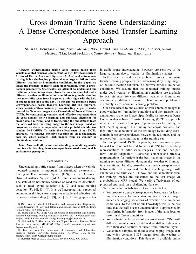
1) Evaluation on Deep Features from Different Layers:We compare different deep representations of our traffic sceneimages extracted from three different layers: the last convo-lutional layer (after pooling), the first fully-connected layer(fc6 layer) and the second fully-connected layer (fc7 layer)of AlexNet and VGG-VD-16 pre-trained on ILSVRC-2012.For the AlexNet, we first reshape the 6 × 6 × 256 mapsfrom the output of the last convolutional layer as the 9,216dimensional vector, and 7×7×512 maps is reshaped as 25,088dimensional vector for VGG-VD-16. For the two networks,4,096 dimensional vector is obtained from the two fully-connected layer. All of the vectors are L2-normalized, andthese vectors are chosen as the feature vectors. The recognitionresults (CMC curves) based on these feature vectors for all ofthe pair-wise domains are shown in Fig. 7. As can be seen inFig. 7, for the two networks, features of the last convolutionallayer get the best performance followed by the fc6 layer andthe fc7 layer. The architectures of VGG-M and VGG-S aresimilar to AlexNet. We use AlexNet and VGG-VD-16 tocompare the feature discrimination of different layers.

2) Evaluation on Different Pre-trained CNNs: To comparedifferent pre-trained CNNs, we extract deep representationsfrom the last convolutional layer in the AlexNet, VGG-M,VGG-S and VGG-VD-16 which are pre-trained on ILSVRC-2012. As shown in Fig. 8, the AlexNet, VGG-M and VGG-S all have good performance on various pair-wise domains.To our surprise, the VGG-VD-16 has the worst performance.Karen Simonyan et al [24] have shown that the very deep fea-tures have a good generalization when transferred to PASCAL


Rank0 10 20 30 40 50 60 70

Cum

ulat

ive

Mat

chin

g S

core

(%)

0

0.1

0.2

0.3

0.4

0.5

0.6

0.7

0.8

0.9

1

last convolution layerfc6 layerfc7 layer

Rank0 10 20 30 40 50 60 70

Cum

ulat

ive

Mat

chin

g S

core

(%)

0

0.1

0.2

0.3

0.4

0.5

0.6

0.7

0.8

0.9

1


Rank0 10 20 30 40 50 60 70

Cum

ulat

ive

Mat

chin

g S

core

(%)

0

0.1

0.2

0.3

0.4

0.5

0.6

0.7

0.8

0.9

1


0 2 4 6 8 10 12 14 16 18 20

Rank

0.4

0.5

0.6

0.7

0.8

0.9

1

Cum

ulat

ive

Mat

chin

g S

core

(%)


Rank0 2 4 6 8 10 12 14 16 18 20

Cum

ulat

ive

Mat

chin

g S

core

(%)

0.7

0.75

0.8

0.85

0.9

0.95

1


sunny day−→ rainy night sunny day−→ night cloudy day−→ rainy night sunny day−→ foggy day sunny day−→ snowy day

Rank0 10 20 30 40 50 60 70

Cum

ulat

ive

Mat

chin

g S

core

(%)

0

0.1

0.2

0.3

0.4

0.5

0.6

0.7

0.8

0.9

1


Rank0 10 20 30 40 50 60 70

Cum

ulat

ive

Mat

chin

g S

core

(%)

0

0.1

0.2

0.3

0.4

0.5

0.6

0.7

0.8

0.9

1


Rank0 10 20 30 40 50 60 70

Cum

ulat

ive

Mat

chin

g S

core

(%)

0

0.1

0.2

0.3

0.4

0.5

0.6

0.7

0.8

0.9

1


Rank0 2 4 6 8 10 12 14 16 18 20

Cum

ulat

ive

Mat

chin

g S

core

(%)

0.7

0.75

0.8

0.85

0.9

0.95

1


Rank0 2 4 6 8 10 12 14 16 18 20

Cum

ulat

ive

Mat

chin

g S

core

(%)

0.7

0.75

0.8

0.85

0.9

0.95

1


cloudy day−→ night snowy day−→ rainy night snowy day−→ night cloudy day−→ snowy day rainy night−→ nightResults for high contrast domains Results for low contrast domains

AlexNet

Rank0 10 20 30 40 50 60 70

Cum

ulat

ive

Mat

chin

g S

core

(%)

0

0.1

0.2

0.3

0.4

0.5

0.6

0.7

0.8

0.9

1


Rank0 10 20 30 40 50 60 70

Cum

ulat

ive

Mat

chin

g S

core

(%)

0

0.1

0.2

0.3

0.4

0.5

0.6

0.7

0.8

0.9

1


Rank0 10 20 30 40 50 60 70

Cum

ulat

ive

Mat

chin

g S

core

(%)

0

0.1

0.2

0.3

0.4

0.5

0.6

0.7

0.8

0.9

1


0 2 4 6 8 10 12 14 16 18 20

Rank

0.2

0.3

0.4

0.5

0.6

0.7

0.8

0.9

1

Cum

ulat

ive

Mat

chin

g S

core

(%)


Rank0 2 4 6 8 10 12 14 16 18 20

Cum

ulat

ive

Mat

chin

g S

core

(%)

0.4

0.5

0.6

0.7

0.8

0.9

1



Rank0 10 20 30 40 50 60 70

Cum

ulat

ive

Mat

chin

g S

core

(%)

0

0.1

0.2

0.3

0.4

0.5

0.6

0.7

0.8

0.9

1


Rank0 10 20 30 40 50 60 70

Cum

ulat

ive

Mat

chin

g S

core

(%)

0

0.1

0.2

0.3

0.4

0.5

0.6

0.7

0.8

0.9

1


Rank0 10 20 30 40 50 60 70

Cum

ulat

ive

Mat

chin

g S

core

(%)

0

0.1

0.2

0.3

0.4

0.5

0.6

0.7

0.8

0.9

1


Rank0 2 4 6 8 10 12 14 16 18 20

Cum

ulat

ive

Mat

chin

g S

core

(%)

0.4

0.5

0.6

0.7

0.8

0.9

1


Rank0 2 4 6 8 10 12 14 16 18 20

Cum

ulat

ive

Mat

chin

g S

core

(%)

0.3

0.4

0.5

0.6

0.7

0.8

0.9

1



VGG-VD-16

Fig. 7. Recognition results with different layers. For the two networks i.e. AlexNet [22] and VGG-VD-16 [24] experimented in various pair-wise domainsof our traffic scene dataset, features of the last convolutional layer achieve the best results followed by the fc6 layer and then the fc7 layer.

VOC-2007 and VOC-2012 benchmarks [57], and image classi-fication benchmarks of Caltech-101 [58] and Caltech-256 [59].Therefore, we should look at what kinds of pretraining areuseful for what tasks.

3) Evaluation on CNNs which are Pre-trained on DifferentData Sets: To compare the performance of deep represen-tations extracted from CNNs pre-trained on different datasets, we use the last convolutional layer of the AlexNetwhich are pre-trained on ILSVRC-2012 [30], Places [23] andPlaces2 [31]. We also test the deep representations extractedfrom AlexNet pre-trained on the data set combining Placeswith ILSVRC-2012 released by MIT Places team. As canbe seen in Fig. 8, for high contrast domains, the datasetcombining Places with ILSVRC-2012 (1,183 categories) hasthe best performance. In contrast, there are no significantdifferences among different large data sets for the low contrastdomains.

C. Evaluation on Effects of Fine-tuning CNNWe fine-tune AlexNet pre-trained on a combined data sets

of ILSVRC-2012 and Places on our traffic scene data set by

using the Caffe framework. We predict 226 or 349 classes forthe traffic scene data sets instead of 1,183 for the pre-traineddata set. We train the last layer only initialized from randomweights. To avoid over-fitting, we use data augmentation asmentioned in Section III-A. We set the initial learning rate as0.0001 decreasing it by an order of magnitude every 10,000iterations. We choose the model of 40,000 iterations. We showthe performance before and after fine-tuning in Table II. Weselect the Rank-1, Rank-5 and Rank-10 for comparison. Theprecision is improved after fine-tuning, particularly the highcontrast pair-wise domains are improved significantly, e.g. 9.4percent improvement for Rank-1 of the cloudy day−→ rainynight.

D. Comparison Deep Representation and Domain Adaptationwith State-of-the-Art

1) Comparison Deep Representations With/without DomainAdaptation: Our traffic scene images may undergo very largeappearance variations. The domain-invariant transformation islearned by using the labeled training data from two domains.


Rank0 5 10 15 20 25 30 35 40

Cum

ulat

ive

Mat

chin

g S

core

(%)

0.3

0.4

0.5

0.6

0.7

0.8

0.9

1

AlexNetVGG-VD-16VGG-MVGG-S

Rank0 5 10 15 20 25 30 35 40

Cum

ulat

ive

Mat

chin

g S

core

(%)

0.2

0.3

0.4

0.5

0.6

0.7

0.8

0.9

1


Rank0 5 10 15 20 25 30 35 40

Cum

ulat

ive

Mat

chin

g S

core

(%)

0.3

0.4

0.5

0.6

0.7

0.8

0.9

1


0 2 4 6 8 10 12 14 16 18 20

Rank

0.6

0.65

0.7

0.75

0.8

0.85

0.9

0.95

1

Cum

ulat

ive

Mat

chin

g S

core

(%)


Rank0 2 4 6 8 10 12 14 16 18 20

Cum

ulat

ive

Mat

chin

g S

core

(%)

0.8

0.82

0.84

0.86

0.88

0.9

0.92

0.94

0.96

0.98

1



Rank0 5 10 15 20 25 30 35 40

Cum

ulat

ive

Mat

chin

g S

core

(%)

0.2

0.3

0.4

0.5

0.6

0.7

0.8

0.9

1


Rank0 5 10 15 20 25 30 35 40

Cum

ulat

ive

Mat

chin

g S

core

(%)

0.2

0.3

0.4

0.5

0.6

0.7

0.8

0.9

1


Rank0 5 10 15 20 25 30 35 40

Cum

ulat

ive

Mat

chin

g S

core

(%)

0.2

0.3

0.4

0.5

0.6

0.7

0.8

0.9

1


Rank0 2 4 6 8 10 12 14 16 18 20

Cum

ulat

ive

Mat

chin

g S

core

(%)

0.8

0.82

0.84

0.86

0.88

0.9

0.92

0.94

0.96

0.98

1


Rank0 2 4 6 8 10 12 14 16 18 20

Cum

ulat

ive

Mat

chin

g S

core

(%)

0.8

0.82

0.84

0.86

0.88

0.9

0.92

0.94

0.96

0.98

1



Recognition results for different networks

Rank0 5 10 15 20 25 30 35 40

Cum

ulat

ive

Mat

chin

g S

core

(%)

0.3

0.4

0.5

0.6

0.7

0.8

0.9

1

ILSVRC2012PlacesPlaces2Places+ILSVRC2012

Rank0 5 10 15 20 25 30 35 40

Cum

ulat

ive

Mat

chin

g S

core

(%)

0.3

0.4

0.5

0.6

0.7

0.8

0.9

1


Rank0 5 10 15 20 25 30 35 40

Cum

ulat

ive

Mat

chin

g S

core

(%)

0.3

0.4

0.5

0.6

0.7

0.8

0.9

1


0 2 4 6 8 10 12 14 16 18 20

Rank

0.7

0.75

0.8

0.85

0.9

0.95

1

Cum

ulat

ive

Mat

chin

g S

core

(%)


Rank0 2 4 6 8 10 12 14 16 18 20

Cum

ulat

ive

Mat

chin

g S

core

(%)

0.9

0.91

0.92

0.93

0.94

0.95

0.96

0.97

0.98

0.99

1



Rank0 5 10 15 20 25 30 35 40

Cum

ulat

ive

Mat

chin

g S

core

(%)

0.3

0.4

0.5

0.6

0.7

0.8

0.9

1


Rank0 5 10 15 20 25 30 35 40

Cum

ulat

ive

Mat

chin

g S

core

(%)

0.3

0.4

0.5

0.6

0.7

0.8

0.9

1


Rank0 5 10 15 20 25 30 35 40

Cum

ulat

ive

Mat

chin

g S

core

(%)

0.3

0.4

0.5

0.6

0.7

0.8

0.9

1


Rank0 2 4 6 8 10 12 14 16 18 20

Cum

ulat

ive

Mat

chin

g S

core

(%)

0.9

0.91

0.92

0.93

0.94

0.95

0.96

0.97

0.98

0.99

1


Rank0 2 4 6 8 10 12 14 16 18 20

Cum

ulat

ive

Mat

chin

g S

core

(%)

0.9

0.91

0.92

0.93

0.94

0.95

0.96

0.97

0.98

0.99

1



Recognition results for different datasets

Fig. 8. Recognition results with different networks/datasets. For different networks, the AlexNet, VGG-M [28] and VGG-S [28] have good performancewhile the VGG-VD-16 has the worst performance. As for different datasets, the dataset combined Places [23] with ILSVRC-2012 [30] obtains the best resultfor high contrast domains, which contains the most categories i.e. 1,183 categories.

TABLE IIPERFORMANCE BEFORE/AFTER FINE-TUNING(%).

Pair-wise domains Before AfterRank 1 Rank 5 Rank 10 Rank 1 Rank 5 Rank 10

sunny day−→ night 44.2 74.6 85.8 47.3 77.6 88.8sunny day−→ rainy night 45.7 79.1 89.6 52.5 82.7 90.2snowy day−→ night 40.2 70.4 83.6 46.5 73.4 84.3snowy day−→ rainy night 41.8 72.0 83.4 51.2 75.1 84.6cloudy day−→ night 45.3 78.1 87.7 48.0 81.0 89.6cloudy day−→ rainy night 48.8 78.4 88.9 58.2 83.5 91.4sunny day−→ snowy day 95.0 98.5 99.6 97.0 98.8 99.6sunny day−→ foggy day 86.4 98.9 99.2 88.6 99.3 99.5cloudy day−→ snowy day 93.4 98.0 99.1 93.8 98.0 99.3rainy night−→ night 95.0 98.6 99.7 96.7 99.4 100

The performance of deep representations before/after cross-domain transformation is compared, as illustrated in Fig. 9. Ascan be seen in Fig. 9, the performance of deep representationsis improved substantially after utilizing the cross-domain trans-formation, e.g. 12.57 percent improvement for Rank-1. Onlyconditions of high contrast domains are considered, which arethe most challenging.

2) Comparison with Local Invariant Features: Local in-variant features have been applied to represent images formatching across appearance changes, e.g. viewpoint and scale.The densely sampled descriptor with compact VLAD encodingis proposed in [17], which has better performance comparedwith repeatable detection of local invariant features for rec-ognizing the same scene across large appearance changes,


0 2 4 6 8 10 12 14 16 18 20

Rank

0.3

0.4

0.5

0.6

0.7

0.8

0.9

1C

umul

ativ

e M

atch

ing

Sco

re(%

)

After:sunny-nightAfter:cloudy-nightAfter:snowy-nightBefore:sunny-nightBefore:cloudy-nightBefore:snowy-night

0 2 4 6 8 10 12 14 16 18 20

Rank

0.3

0.4

0.5

0.6

0.7

0.8

0.9

1

Cum

ulat

ive

Mat

chin

g S

core

(%)

After:sunny-rainyAfter:cloudy-rainyAfter:snowy-rainyBefore:sunny-rainyBefore:cloudy-rainyBefore:snowy-rainy

daytime−→night daytime−→rainy night

Fig. 9. Comparison deep representations before/after cross-domain transfor-mation.

Rank0 10 20 30 40 50 60 70

Cum

ulat

ive

Mat

chin

g S

core

(%)

0

0.1

0.2

0.3

0.4

0.5

0.6

0.7

0.8

0.9

1

CNN:cloudy-nightVLAD:cloudy-nightCNN:snowy-nightVLAD:snowy-nightCNN:sunny-nightVLAD:sunny-night

Rank0 10 20 30 40 50 60 70

Cum

ulat

ive

Mat

chin

g S

core

(%)

0

0.1

0.2

0.3

0.4

0.5

0.6

0.7

0.8

0.9

1

CNN:cloudy-rainyVLAD:cloudy-rainyCNN:snowy-rainyVLAD:snowy-rainyCNN:sunny-rainyVLAD:sunny-rainy

Fig. 10. Comparison with local invariant features. For different challengingscenarios, i.e. the high contrast domains shown in Table 1.

e.g. illumination (day and night times). We compare our deeprepresentations extracted from fine-tuned CNN with this localinvariant features. The dense VLAD descriptors of the trafficscene images are computed according to [17].

We compute the dense VLAD descriptors on the originalimages, rather than after resizing each image to maximumdimension as in [17]. The visual vocabulary of 128 visualwords is built from descriptors randomly sampled from ourtraffic scene dataset using k-means clustering. We fine-tune theCNN using images from our traffic scene data sets. It is helpfulto compare the dense VLAD with CNN descriptors on thesame level. Unlike [17], the dense VLAD descriptors are notcompressed by using PCA because our method uses a way ofdimension reduction more robust than PCA. We use the sametransformation for comparing different image representations.

Fig. 10 shows the recognition results of different imagerepresentations. As can be seen in Fig. 10, the performance ofCNN descriptors is better than the dense VLAD descriptors,e.g. 35.67 percent for Rank-1 improvement by using CNNdescriptors. These results demonstrate that our method iseffective for scene recognition in challenging conditions.

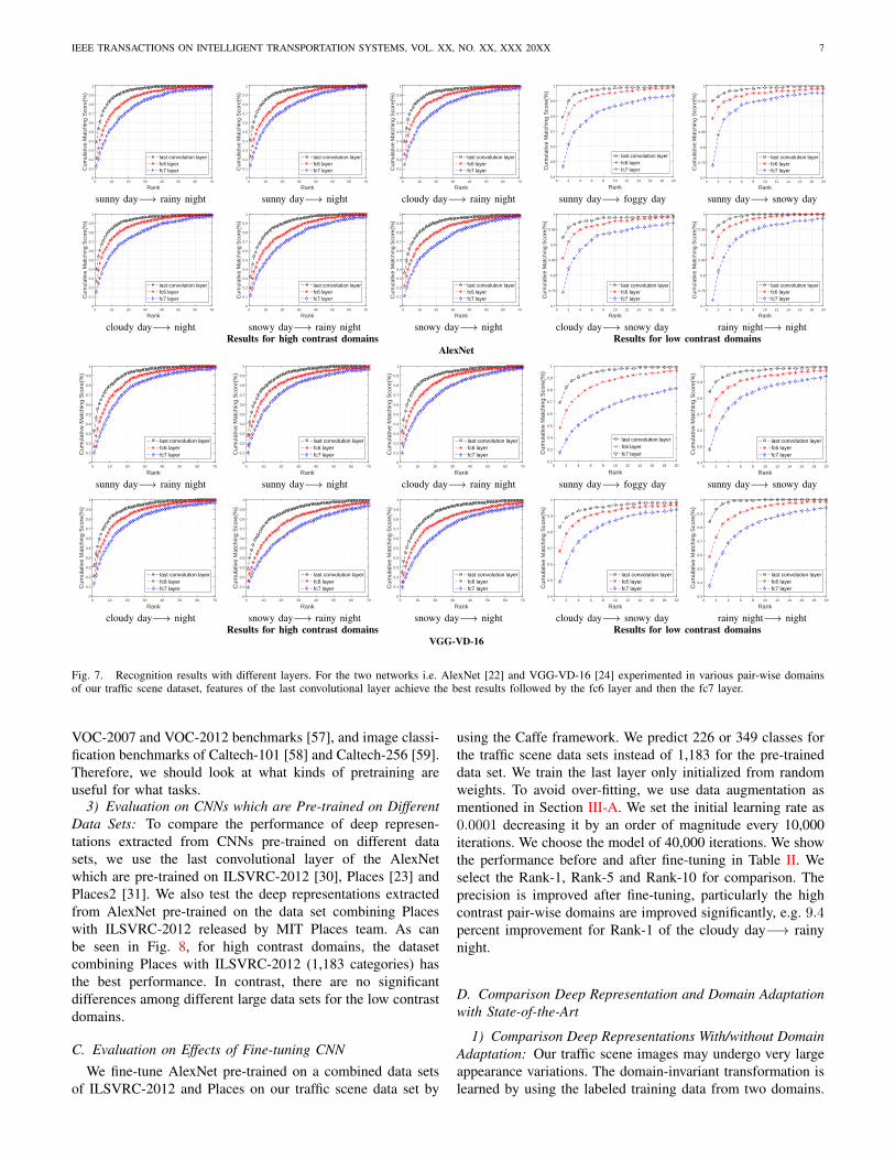
3) Comparison with Subspace Based TransformationLearning Methods: For subspace based transformation learn-ing, we compare our method with two state-of-the-art methodsi.e. Geodesic Flow Kernel (GFK) [19] and Subspace Align-ment (SA) [18] on our traffic scene data sets. For GFK,the intermediate subspaces are learned along the geodesicdirection from one domain to another domain. As for SA, thetransformation is learned between subspaces of two domains.For all of the transformation learning methods, the deeprepresentations extracted from the fine-tuned network are usedas the input image representations.

As can be seen in Fig. 11, our method has the best perfor-mance compared to the state-of-the-art methods. Our method

outperforms SA and GFK methods in the high contrast do-mains. As for the low contrast domains, our method performsslightly better than them. Our method has better performancecomparing with the state-of-the-art subspace based methods,particularly for traffic scene images undergoing significantappearance variations.

E. Scene Understanding Results

In this subsection, we conduct the quantitative and qual-itative traffic scene understanding experiments. Specifically,for ten different pair-wise domains shown in Table I, halfdata from each domain are used for learning the cross-domaintransformation. Then, the label transfer method is verified onthe other half data from each domain. We retrieve κ = 1 imagefor each test image in the target domain. The average per-classand per-pixel rates6 for each condition are shown in Table III.

The major challenge for traffic scene understanding isnon-uniform statistics of object categories in a traffic scene.“Texture” classes, such as road, sky, tree etc., constitute themajority of the image pixels, which have no consistent shapebut consistent texture. In contrast, “object” classes whichare characterized by overall shape occupy a small percent-age of the image pixels, e.g. traffic signs, traffic lights andpoles. As shown in Table III, for the low contrast domainsboth object classes (“Bridge”, “Median Strip”, “Car”, “TrafficSign”, “Traffic Lights” and “Pole”) and texture categories(“Building”, “Road”, “Tree”, “Sky” and “Vegetation”) havegood performance. However, for the high contrast domainsthe performance is decreased especially for the object classes.The recognition rates of poles and traffic signs are significantlydifferent between high and low contrast domains. The mainreason is that there are drastic illumination changes for highcontrast domains. We show qualitative results in Fig. 12 and13.

F. Running Time and Implementation Environment

In Table IV we show the running time of each part andthe implementation environment/programming language of theproposed algorithm. The fine-tuning is conducted on NVIDIAEVGA GeForce GTX TITAN X GPU by using Caffe frame-work. Transformation learning, image retrieval (i.e. finding thematching image in another domain given the test image) andlabel transfer are tested on Intel Core i7-4770 CPU with 16GB of RAM in Matlab/C++ implementation. As can shownin Table IV, the fine-tuning and domain transformation arelearned off-line, and the pre-learned models are used in realtraffic. Currently it takes less than two seconds to understandone test image. Further speedup could be achieved throughGPU implementation in future work. The dense correspon-dence/label transfer is implemented by using the methodfrom [60], greatly speeding up the inference.

6Images in the target domain are interpreted by label transfer from thesource domain. Hence, it would be meaningful to compute the recognitionrates for categories which are jointly “owned” by different weather conditions.For example, as can be seen in Fig. 6, the wiper class is only included in snowyday. The recognition rates of 11 classes owned by all weather conditions arereported in Table III, and the recognition results for pedestrian and wiper arenot included.


Rank0 5 10 15 20 25 30 35 40

Cum

ulat

ive

Mat

chin

g S

core

(%)

0.4

0.5

0.6

0.7

0.8

0.9

1

GFKSAOurs

Rank0 5 10 15 20 25 30 35 40

Cum

ulat

ive

Mat

chin

g S

core

(%)

0.3

0.4

0.5

0.6

0.7

0.8

0.9

1

GFKSAOurs

Rank0 5 10 15 20 25 30 35 40

Cum

ulat

ive

Mat

chin

g S

core

(%)

0.5

0.55

0.6

0.65

0.7

0.75

0.8

0.85

0.9

0.95

1

GFKSAOurs

0 1 2 3 4 5 6 7 8 9 10

Rank

0.85

0.9

0.95

1

Cum

ulat

ive

Mat

chin

g S

core

(%)

GFKSAOurs

Rank0 1 2 3 4 5 6 7 8 9 10

Cum

ulat

ive

Mat

chin

g S

core

(%)

0.95

0.955

0.96

0.965

0.97

0.975

0.98

0.985

0.99

0.995

1

GFKSAOurs


Rank0 5 10 15 20 25 30 35 40

Cum

ulat

ive

Mat

chin

g S

core

(%)

0.4

0.5

0.6

0.7

0.8

0.9

1

GFKSAOurs

Rank0 5 10 15 20 25 30 35 40

Cum

ulat

ive

Mat

chin

g S

core

(%)

0.4

0.5

0.6

0.7

0.8

0.9

1

GFKSAOurs

Rank0 5 10 15 20 25 30 35 40

Cum

ulat

ive

Mat

chin

g S

core

(%)

0.4

0.5

0.6

0.7

0.8

0.9

1

GFKSAOurs

Rank0 1 2 3 4 5 6 7 8 9 10

Cum

ulat

ive

Mat

chin

g S

core

(%)

0.9

0.91

0.92

0.93

0.94

0.95

0.96

0.97

0.98

0.99

1

GFKSAOurs

Rank0 1 2 3 4 5 6 7 8 9 10

Cum

ulat

ive

Mat

chin

g S

core

(%)

0.95

0.955

0.96

0.965

0.97

0.975

0.98

0.985

0.99

0.995

1

GFKSAOurs

cloudy day−→ night snowy day−→ rainy night snowy day−→ night cloudy day−→ snowy day rainy night−→ night

Results for high contrast domains Results for low contrast domains

Fig. 11. Comparison with different transformation learning methods. For various challenging scenarios, our method outperforms the state-of-the-art methodsi.e. Geodesic Flow Kernel (GFK) [19] and Subspace Alignment (SA) [18].

TABLE IIISCENE UNDERSTANDING RESULTS ON OUR CROSS-DOMAIN TRAFFIC SCENE DATASET (%)

Bridge Building Car MedianStrip Pole Road Sky Traffic

LightsTrafficSign Tree Vegetation Per-class Per-pixel

cloudy day−→snowy day 97.1 91.6 38.9 68.9 84.0 83.0 98.5 80.6 92.3 88.0 66.3 80.8 90.6cloudy day−→rainy night 66.9 71.4 41.7 39.1 39.3 41.9 91.1 33.0 58.8 55.8 15.0 50.4 78.7cloudy day−→night 61.8 61.3 34.5 41.6 15.5 43.5 87.5 17.1 63.1 48.9 10.1 44.1 75.7snowy day−→night 64.2 71.7 33.8 51.1 16.4 57.0 79.6 13.2 53.1 24.3 9.6 43.1 73.1snowy day−→rainy night 80.1 67.7 43.5 51.2 32.2 58.4 81.6 36.5 43.1 38.0 20.8 50.3 72.4rainy night−→night 96.8 86.9 42.4 83.2 54.1 81.4 70.9 89.4 92.0 89.2 12.1 72.6 89.5sunny day−→night 43.6 69.0 31.3 72.4 23.4 67.6 84.7 10.7 56.5 45.7 27.3 48.4 76.9sunny day−→rainy night 42.9 72.9 38.8 68.9 24.2 61.7 80.4 11.0 64.5 48.6 35.8 50.0 72.8sunny day−→snowy day 88.9 90.8 36.7 86.8 78.7 83.3 92.9 47.5 94.9 90.6 68.3 78.1 87.7sunny day−→foggy day - 70.1 31.9 - 51.9 86.7 87.1 10.5 46.3 89.0 - 59.2 86.3

BuildingSky Tree Road Car Median Strip Traffic Sign Pole UndefinedBuildingSky Tree Road Car Median Strip Traffic Sign Pole Undefined

Fig. 12. Some representative scene understanding results of the rainy night scenario. Original images, results for cloudy day−→ rainy night, results forsnowy day−→ rainy night, results for sunny day−→ rainy night and human annotation are shown in each row, respectively (top to bottom).


Building Sky Tree Road Car Traffic Sign Pole Undefined

Fig. 13. Some representative scene understanding results of the foggy day scenario. Original images, results for sunny day−→ foggy day and humanannotation are shown in each row, respectively (top to bottom).

TABLE IVRUNNING TIME (SECOND) AND THE IMPLEMENTATION ENVIRONMENT

Fine-tune Transform learning Image retrieval Label transferRunning time Off-line Off-line 0.31 1.6Environment Caffe Matlab Matlab Matlab/C++

V. CONCLUSION

In this paper we proposed a dense correspondence basedtransfer learning approach. The approach employs a fine-tunedCNN to extract deep features. It performs cross-domain metriclearning and subspace alignment for constructing compact rep-resentations to retrieve the cross-domain best matching image.The approach transfers the annotations from the cross-domainbest matching image to the test image based on the establisheddense correspondences between them. We conducted extensiveexperiments with our new cross-domain traffic scene dataset. Experimental results demonstrated the effectiveness ofour proposed approach. We hope that our work can pave anew way to traffic scene understanding in challenging drivingsituations under varying weather and illumination conditions.

The robustness of our proposed approach is dependent uponthe dense correspondences based on the SIFT flow. As shownin [61], [62], [63], [64], SCNN [65] is of potential valueto learn more powerful representations for finding correspon-dences. We leave this as our future work.

ACKNOWLEDGMENT

This work was supported in part by the National NaturalScience Foundation of China under Grant 61601042, Grant61402047 and Grant 61528204, and in part by the BeijingNatural Science Foundation under Grant 4162044.

REFERENCES

[1] A. Geiger, C. Wojek, and R. Urtasun, “Joint 3d estimation of objectsand scene layout,” in Proc. NIPS, 2011, pp. 1467–1475.

[2] C. Guo, J. Meguro, Y. Kojima, and T. Naito, “A multimodal adas systemfor unmarked urban scenarios based on road context understanding,”IEEE Trans. Intell. Transp. Syst., vol. 16, no. 4, pp. 1690–1704, 2015.

[3] J. C. McCall and M. M. Trivedi, “Video-based lane estimation andtracking for driver assistance: Survey, system, and evaluation,” IEEETrans. Intell. Transp. Syst., vol. 7, no. 1, pp. 20–37, 2006.

[4] Y. He, H.Wang, and B. Zhang, “Color-based road detection in urbantraffic scenes,” IEEE Trans. Intell. Transp. Syst., vol. 5, no. 4, pp. 309–318, 2004.

[5] H. Guan, J. Li, Y. Yu, Z. Ji, and C. Wang, “Using mobile lidar datafor rapidly updating road markings,” IEEE Trans. Intell. Transp. Syst.,vol. 16, no. 5, pp. 2457–2466, 2015.

[6] R. Marc, G. Dominique, and P. Evangeline, “Generator of road markingtextures and associated ground truth applied to the evaluation of roadmarking detection,” in Proc. ITSC, 2012, pp. 933–938.

[7] Y. Kang, K. Yamaguchi, T. Naito, and Y. Ninomiya, “Multiband imagesegmentation and object recognition for understanding road scenes,”IEEE Trans. Intell. Transp. Syst., vol. 12, no. 4, pp. 1423–1433, 2011.

[8] Q. Zou, H. Ling, S. Luo, Y. Huang, and M. Tian, “Robust nighttimevehicle detection by tracking and grouping headlights,” IEEE Trans.Intell. Transp. Syst., vol. 16, no. 5, pp. 2838–2849, 2015.

[9] S. Di, H. Zhang, X. Mei, D. Prokhorov, and H. Ling, “A benchmarkfor cross-weather traffic scene understanding,” in Proc. ITSC, 2016, pp.2150–2156.

[10] ——, “Spatial prior for nonparametric road scene parsing,” in Proc.ITSC, 2015, pp. 1209–1214.

[11] T. Sattler, M. Havlena, F. Radenovic, K. Schindler, and M. Pollefeys,“Hyperpoints and fine vocabularies for large scale location recognition,”in Proc. Int. Conf. Comput. Vis., 2015, pp. 2102–2110.

[12] J. Knopp, J. Sivic, and T. Pajdla, “Avoding confusing features in placerecognition,” in Proc. Eur. Conf. Comput. Vis., 2010, pp. 748–761.

[13] M. Milford, W. J. Scheirer, E. Vig, A. Glover, O. Baumann, J. Mat-tingley, and D. D. Cox, “Condition-invariant, top-down visual placerecognition,” in Proc. IEEE Conf. Robotics and Automation, 2014, pp.5571–5577.

[14] Y. Li, N. Snavely, D. Huttenlocher, and P. Fua, “Worldwide poseestimation using 3d point clouds,” in Proc. Eur. Conf. Comput. Vis.,2012, pp. 15–29.

[15] T. Sattler, B. Leibe, and L. Kobbelt, “Improving image-based localiza-tion by active correspondence search,” in Proc. Eur. Conf. Comput. Vis.,2012, pp. 752–765.

[16] A. R. Zamir and M. Shah, “Accurate image localization based on googlemaps street view,” in Proc. Eur. Conf. Comput. Vis., 2010, pp. 255–268.

[17] A. Torii, R. Arandjelovic, J. Sivic, M. Okutomi, and T. Pajdla, “24/7place recognition by view synthesis,” in Proc. IEEE Conf. Comput. Vis.Pattern Recognit., 2015, pp. 1808–1817.


[18] B. Fernando, A. Habrard, M. Sebban, and T. Tuytelaars, “Unsupervisedvisual domain adaptation using subspace alignment,” in Proc. Int. Conf.Comput. Vis., 2013, pp. 2960–2967.

[19] B. Gong, Y. Shi, F. Sha, and K. Grauman, “Geodesic flow kernel forunsupervised domain adaptation,” in Proc. IEEE Conf. Comput. Vis.Pattern Recognit., 2012, pp. 2066–2073.

[20] R. Aljundi, R. Emonet, D. Muselet, and M. Sebban, “Landmarks-basedkernelized subspace alignment for unsupervised domain adaptation,” inProc. IEEE Conf. Comput. Vis. Pattern Recognit., 2015, pp. 56–63.

[21] R. Gopalan, R. Li, and R. Chellappa, “Domain adaptation for objectrecognition: An unsupervised approach,” in Proc. Int. Conf. Comput.Vis., 2011, pp. 999–1006.

[22] A. Krizhevsky, I. Sutskever, and G. E. Hinton, “Imagenet classificationwith deep convolutional neural networks,” in Proc. NIPS, 2012, pp.1097–1105.

[23] B. Zhou, A. Khosla, A. Lapedriza, A. Torralba, and A. Oliva, “Learningdeep features for scene recognition using places database,” in NIPS,2014, pp. 487–495.

[24] K. Simonyan and A. Zisserman, “Very deep convolutional networks forlarge-scale image recognition,” in Proc. ICLR, 2015.

[25] C. Szegedy, W. Liu, Y. Jia, P. Sermanet, S. Reed, D. Anguelov, D. Erhan,V. Vanhoucke, and A. Rabinovich, “Going deeper with convolutions,”in Proc. IEEE Conf. Comput. Vis. Pattern Recognit., 2015, pp. 1–9.

[26] J. Donahue, Y. Jia, O. Vinyals, J. Hoffman, N. Zhang, E. Tzeng, andT. Darrell, “Decaf: A deep convolutional activation feature for genericvisual recognition,” in Proc. ICML, 2014, pp. 647–655.

[27] M. D. Zeiler and R. Fergus, “Visualizing and understanding convolu-tional networks,” in Proc. Eur. Conf. Comput. Vis., 2014, pp. 818–833.

[28] K. Chatfield, K. Simonyan, A. Vedaldi, and A. Zisserman, “Return ofthe devil in the details: Delving deep into convolutional nets,” in arXivpreprint arXiv:1405.3531, 2014.

[29] A. S. Razavian, H. Azizpour, J. Sullivan, and S. Carlsson, “Cnn featuresoff-the-shelf: an astounding baseline for recognition,” in Proc. IEEEConf. Comput. Vis. Pattern Recognit. DeepVision workshop, 2014, pp.806–813.

[30] J. Deng, W. Dong, R. Socher, L. Li, K. Li, and F. F. Li, “Imagenet: Alarge-scale hierarchical image database,” in Proc. IEEE Conf. Comput.Vis. Pattern Recognit., 2009, pp. 248–255.

[31] B. Zhou, A. Khosla, A. Lapedriza, A. Torralba, and A. Oliva,“Places2: A large-scale database for scene understanding,” inhttp://places2.csail.mit.edu/, 2015.

[32] J. Long, E. Shelhamer, and T. Darrell, “Fully convolutional networksfor semantic segmentation,” in Proc. IEEE Conf. Comput. Vis. PatternRecognit., 2015, pp. 3431–3440.

[33] H. Noh, S. Hong, and B. Han, “Learning deconvolution network forsemantic segmentation,” in Proc. Int. Conf. Comput. Vis., 2015, pp.1520–1528.

[34] S. Zheng, S. Jayasumana, B. R. Paredes, V. Vineet, Z. Su, D. Huang,and P. Torr, “Conditional random fields as recurrent neural networks,”in Proc. Int. Conf. Comput. Vis., 2015, pp. 1529–1537.

[35] D. Eigen and R. Fergus, “Predicting depth, surface normals and semanticlabels with a common multi-scale convolutional architecture,” in Proc.Int. Conf. Comput. Vis., 2015, pp. 2650–2658.

[36] S. Hong, H. Noh, and B. Han, “Decoupled deep neural network for semi-supervised semantic segmentation,” in Proc. NIPS, 2015, pp. 1495–1503.

[37] X. Qi, C.-G. Li, G. Zhao, X. Hong, and M. Pietikainen, “Dynamictexture and scene classification by transferring deep image features,”Neurocomputing, vol. 171, pp. 1230–1241, 2016.

[38] R. Girshick, J. Donahue, T. Darrell, and J. Malik, “Rich featurehierarchies for accurate object detection and semantic segmentation,” inProc. IEEE Conf. Comput. Vis. Pattern Recognit., 2014, pp. 580–587.

[39] M. Oquab, L. Bottou, I. Laptev, and J. Sivic, “Learning and transferringmid-level image representations using convolutional neural networks,”in Proc. IEEE Conf. Comput. Vis. Pattern Recognit., 2014, pp. 1717 –1724.

[40] H. Abdi, “Partial least square regression, projection on latent structureregression, pls-regression,” Wiley Interdisciplinary Reviews: Computa-tional Statistics, vol. 2, pp. 97–106, 2010.

[41] S. Liao and S. Z. Li, “Efficient psd constrained asymmetric metriclearning for person re-identification,” in Proc. Int. Conf. Comput. Vis.,2015, pp. 3685–3693.

[42] B. Fernando, A. Habrard, M. Sebban, and T. Tuytelaars, “Subspacealignment for domain adaptation,” in arXiv preprint arXiv:1409.5241,2014.

[43] C. Liu, J. Yuen, and A. Torralba, “Sift flow: Dense correspondenceacross scenes and its applications,” IEEE Trans. Pattern Anal. Mach.Intell., vol. 33, no. 5, pp. 978–994, 2011.

[44] ——, “Nonparametric scene parsing via label transfer,” IEEE Trans.Pattern Anal. Mach. Intell., vol. 33, no. 12, pp. 2368–2382, 2011.

[45] D. G. Lowe, “Distinctive image features from scale-invariant keypoints,”Int. J. Comput.Vis., vol. 60, no. 2, pp. 91–110, 2004.

[46] J. Long, N. Zhang, and T. Darrell, “Do convnets learn correspondence?”in Proc. NIPS, 2014, pp. 1601–1609.

[47] P. Felzenszwalb and D. P. Huttenlocher, “Efficient belief propagation forearly vision,” Int. J. Comput.Vis., vol. 70, no. 1, pp. 41–54, 2006.

[48] C. Liu, J. Yuen, and A. Torralba, “Nonparametric scene parsing: labeltransfer via dense scene alignment,” in Proc. IEEE Conf. Comput. Vis.Pattern Recognit., 2009, pp. 1972–1979.

[49] C. Rother, V. Kolmogorov, and A. Blake, “Grabcut-interactive fore-ground extraction using iterated graph cuts,” ACM Transactions onGraphics, vol. 23, no. 3, pp. 309–314, 2004.

[50] B. Russell, A. Torralba, K. Murphy, and W. T. Freeman, “Labelme: adatabase and web-based tool for image annotation,” Int. J. Comput.Vis.,vol. 77, no. 1, pp. 157–173, 2008.

[51] W. Zheng, X. Li, T. Xiang, S. Liao, J. Lai, and S. Gong, “Partial personre-identification,” in Proc. Int. Conf. Comput. Vis., 2015, pp. 4678–4686.

[52] J. Tighe and S. Lazebnik, “Superparsing: Scalable nonparametric imageparsing with superpixels,” Int. J. Comput.Vis., vol. 101, no. 2, pp. 329–349, 2013.

[53] J. Yang, B. Price, S. Cohen, and M. Yang, “Context driven scene parsingwith attention to rare classes,” in Proc. IEEE Conf. Comput. Vis. PatternRecognit., 2014, pp. 3294–3301.

[54] J. Tighe, M. Niethammer, and S. Lazebnik, “Scene parsing with objectinstances and occlusion ordering,” in Proc. IEEE Conf. Comput. Vis.Pattern Recognit., 2014, pp. 3748–3755.

[55] Y. Jia, “Caffe: An open source convolutional architecture for fast featureembedding. http://caffe.berkeleyvision.org/,” 2013.

[56] P. Sermanet, D. Eigen, X. Zhang, M. Mathieu, R. Fergus, and Y. Le-Cun, “Overfeat:integrated recognition, localization and detection usingconvolutional networks,” in Proc. ICLR, 2014, p. 16.

[57] M. Everingham, S. Eslami, L. V. Gool, C. Williams, J. Winn, and A. Zis-serman, “The pascal visual object classes challenge: a retrospective,” Int.J. Comput.Vis., vol. 111, no. 1, pp. 98–136, 2015.

[58] F. F. Li, R. Fergus, and P. Perona, “Learning generative visual modelsfrom few training examples: An incremental bayesian approach testedon 101 object categories,” in Proc. IEEE Conf. Comput. Vis. PatternRecognit. Workshop of Generative Model Based Vision, 2004, p. 178.

[59] G. Griffinand, A. Holub, and P. Perona, “Caltech-256 object categorydataset,” in Technical Report 7694, California Institute of Technology,2007.

[60] J. Kim, C. Liu, F. Sha, and K. Grauman, “Deformable spatial pyramidmatching for fast dense correspondences,” in Proc. IEEE Conf. Comput.Vis. Pattern Recognit., 2013, pp. 2307–2314.

[61] P. Agrawal, J. Carreira, and J. Malik, “Learning to see by moving,” inProc. Int. Conf. Comput. Vis., 2015, pp. 37–45.

[62] J. Flynn, I. Neulander, J. Philbin, and N. Snavely, “Deepstereo: Learningto predict new views from the world’s imagery,” in Proc. IEEE Conf.Comput. Vis. Pattern Recognit., 2016, pp. 5515–5524.

[63] D. Jayaraman and K. Grauman, “Learning image representations tied toego-motion,” in Proc. Int. Conf. Comput. Vis., 2015, pp. 1413–1421.

[64] J. Zbontar and Y. LeCun, “Stereo matching by training a convolutionalneural network to compare image patches,” Journal of Machine LearningResearch, vol. 17, no. 1, pp. 1–32, 2016.

[65] S. Chopra, R. Hadsell, and Y. LeCun, “Learning a similarity metricdiscriminatively, with application to face verification,” in Proc. IEEEConf. Comput. Vis. Pattern Recognit., 2005, pp. 539–546.

Shuai Di is a PhD student jointly training in the Bei-jing University of Posts and Telecommunications,and the Department of Computer and InformationSciences, Temple University. His research interestsinclude computer vision and pattern recognition andtheir applications in intelligent vehicles.


Honggang Zhang (SM’12) received the B.S. de-gree from the Department of Electrical Engineering,Shandong University, in 1996, the masters and Ph.D.degrees from the School of Information Engineering,Beijing University of Posts and Telecommunications(BUPT), in 1999 and 2003, respectively. He wasa Visiting Scholar with the School of ComputerScience, Carnegie Mellon University, from 2007 to2008. He is currently an Associate Professor and theDirector of Web Search Center with BUPT. He pub-lished more than 30 papers on TPAMI, SCIENCE,

Machine Vision and Applications, AAAI, ICPR, ICIP. His research interestsinclude image retrieval, computer vision, and pattern recognition.

Chun-Guang Li received the B.E. degree intelecommunication engineering from the Jilin Uni-versity in 2002 and the Ph.D. degree in signalprocessing from the Beijing University of Posts andTelecommunications (BUPT) in 2007. Currently, heis an associate professor with the School of In-formation and Communication Engineering, BUPT.From July 2011 to April 2012, he visited the VisualComputing group, Microsoft Research Asia. FromDecember 2012 to November 2013, he visited theVision, Dynamics, and Learning lab, the Johns Hop-

kins University. His research interests are statistical signal processing andmachine learning. He is a member of the IEEE, ACM, and CCF.

Xue Mei (SM’14) received the B.S. degree in elec-trical engineering from the University of Science andTechnology of China, Hefei, China, and the Ph.D.degree in electrical engineering from the Universityof Maryland, College Park, MD, USA. He was withthe Automation Path-Finding Group in Assemblyand Test Technology Development and the VisualComputing Group, Intel Corporation, USA, from2008 to 2012. He is currently a Senior ResearchScientist with the Future Mobility Research Depart-ment, Toyota Research Institute, Ann Arbor, MI,

USA, a Toyota Technical Center division. He serves as an Adjunct Professorwith Anhui University, Hefei. His current research interests include computervision, machine learning, and robotics with a focus on intelligent vehiclesresearch. Dr. Mei was an Area Chair of the Winter Conference on ComputerVision in 2015 and 2016, and a Lead Organizer of the My Car Has Eyes:Intelligent Vehicle With Vision Technology Workshop at the Asian Conferenceon Computer Vision in 2014. He serves as a Lead Guest Editor of the SpecialIssue on Visual Tracking of Computer Vision and Image Understanding.

Danil Prokhorov (SM’02) was a Research Engineerwith the St. Petersburg Institute for Informaticsand Automation, Russian Academy of Sciences,Saint Petersburg, Russia. He has been involved inautomotive research since 1995. He was an In-tern with the Scientific Research Laboratory, FordMotor Company, Dearborn, MI, USA, in 1995. In1997, he became a Research Staff Member withFord Motor Company, where he was involved inapplication-driven research on neural networks andother machine learning methods. Since 2005, he

has been with the Toyota Technical Center, Ann Arbor, MI, USA. He iscurrently in charge of the Department of Future Mobility Research, ToyotaResearch Institute, Ann Arbor. He has authored over 100 papers in variousjournals and conference proceedings and holds many patents in a varietyof areas. Dr. Prokhorov served as the International Neural Network SocietyPresident from 2013 to 2014, and was a member of the IEEE IntelligentTransportation Systems Society Board of Governors, a U.S. National ScienceFoundation Expert, and an Associate Editor/Program Committee Member ofmany international journals and conferences.

Haibin Ling received the B.S. degree in mathe-matics and the M.S. degree in computer sciencefrom Peking University, China, in 1997 and 2000,respectively, and the Ph.D. degree in computer sci-ence from the University of Maryland, College Park,in 2006. From 2000 to 2001, he was an AssistantResearcher with Microsoft Research Asia. From2006 to 2007, he was a Post-Doctoral Scientist withthe University of California at Los Angeles. Afterthat, he joined Siemens Corporate Research as aResearch Scientist. Since Fall 2008, he has been with

Temple University, where he is currently an Associate Professor. His researchinterests include computer vision, medical image analysis, human-computerinteraction, and machine learning. He received the Best Student Paper Awardat the ACM Symposium on User Interface Software and Technology in 2003,and the NSF CAREER Award in 2014. He has served on the editorial boardof IEEE Trans. on Pattern Analysis and Machine Intelligence and PatternRecognition, and Area Chairs for CVPR 2014 and CVPR 2016.

Documents

IEEE TRANSACTIONS ON INTELLIGENT …hbling/publication/TITS_04092017-L.pdf · A Dense Correspondence based Transfer Learning Approach Shuai Di, Honggang Zhang, Senior Member, IEEE,