IEEE TRANSACTIONS ON INTELLIGENT TRANSPORTATION SYSTEMS 1

B-Planner: Planning Bidirectional Night Bus RoutesUsing Large-scale Taxi GPS Traces

Chao Chen, Daqing Zhang, Nan Li, and Zhi-Hua Zhou, Fellow, IEEE

Abstract—Taxi GPS traces can inform us the human mobilitypatterns in modern cities. Instead of leveraging the costly andinaccurate human surveys about people’s mobility, we intendto explore the night bus route planning issue by using taxiGPS traces. Specifically, we propose a two-phase approach forbi-directional night-bus route planning. In the first phase, wedevelop a process to cluster “hot” areas with dense passengerpick-up/drop-off, and then propose effective methods to splitbig “hot” areas into clusters and identify a location in eachcluster as a candidate bus stop. In the second phase, giventhe bus route origin, destination, candidate bus stops as wellas bus operation time constraints, we derive several effectiverules to build the bus route graph, and prune invalid stopsand edges iteratively. Based on this graph, we further developa Bi-directional Probability based Spreading (BPS) algorithm togenerate candidate bus routes automatically. We finally selectthe best bi-directional bus route which expects the maximumnumber of passengers under the given conditions and constraints.To validate the effectiveness of the proposed approach, extensiveempirical studies are performed on a real-world taxi GPS data setwhich contains more than 1.57 million night passenger deliverytrips, generated by 7,600 taxis in a month.

Index Terms—Taxi GPS Traces; Human Mobility Patterns;Route Graph; Bus Route Planning

I. INTRODUCTION

BUses are a popular and economical way for people totravel around the city, and they are generally “greener”

than cars and taxis as they help decrease traffic congestion,fuel consumption, carbon dioxide emission and travel cost [1].Thus for sustainable city development, people are encouragedto take public transportation for work, visit, etc.. In manycities, the daytime bus transportation systems are usually welldesigned; however, during late nights, most bus systems areout of service, leaving taxis as the only option for intra-citytravelling. To provide cost-effective and environment friendlytransport to citizens, many cities start to plan night-throughbus routes.

Previously, bus route planning mainly relied on humansurveys to understand people’s mobility patterns [5], [19].

Chao Chen is with the CNRS UMR 5157 SAMOVAR, Institut Mines-TELECOM/TELECOM SudParis, Evry 91011, France, and also with theDepartment of Computer, Universite Pierre et Marie CURIE, 4 place Jussieu75005 Paris, France (e-mail: chao.chen@telecom-sudparis.eu)

Daqing Zhang is with the the CNRS UMR 5157 SAMOVAR, Insti-tut Mines-TELECOM/TELECOM SudParis, Evry 91011, France (e-mail:daqing.zhang@telecom-sudparis.eu)

Nan Li is with the National Key Laboratory for Novel Software Technology,Nanjing University, Nanjing 210023, China, and also with the School ofMathematical Sciences, Soochow University, Suzhou 215006, China (e-mail:lin@lamda.nju.edu.cn)

Zhi-Hua Zhou is with the National Key Laboratory for Novel Soft-ware Technology, Nanjing University, Nanjing 210023, China (e-mail:zhouzh@lamda.nju.edu.cn)

Although this approach was proved to be workable, the timeand cost spent in the survey process were quite substantial.Moreover, such an approach is not able to accommodate thefrequent change in the road network and traffic, especiallyfor cities which experience rapid development. With the widedeployment of GPS devices and wireless communication intaxis, rich information about taxis including where and whenpassengers are picked-up or dropped-off, which route a taxitakes for a certain trip, can be collected and extracted. Know-ing the origin-destination (OD) of each taxi trip providesvaluable information to understand passengers’ mobility flowin a city at different time of a day, making it possibleto accurately plan new night-bus routes which expect themaximum number of passengers along the routes.

In this paper, we intend to explore the bi-directional night-bus route design problem leveraging the taxi GPS traces. Thisproblem can be divided into two sub-problems: the candidatebus stop identification and the best bi-directional bus routeselection. For the first sub-problem, we need to identify thecandidate bus stops which are associated with locations havingbig number of taxi passenger pick-up and drop-off records(PDRs), the bus stops should be evenly distributed in the “hot”districts to facilitate people’s access. After the candidate busstops are identified, the next step is to select a bi-directionalbus route which connects the bus origin and a sequence ofbus stops to the destination, expecting the maximum numberof passengers in both directions given a specific bus operationtime, frequency and total travel time. Fortunately, the taxiGPS traces contain quantitative spatial-temporal informationabout all taxi trips. By mining the taxi GPS data, we caninform where are the “hot” areas for taxi passengers andhow many passengers would potentially travel along a certainroute in a specific time duration. Therefore, the bi-directionalnight-bus route design becomes a problem of comparing thenumber of passengers of all valid bus routes giving certaintime constraints.

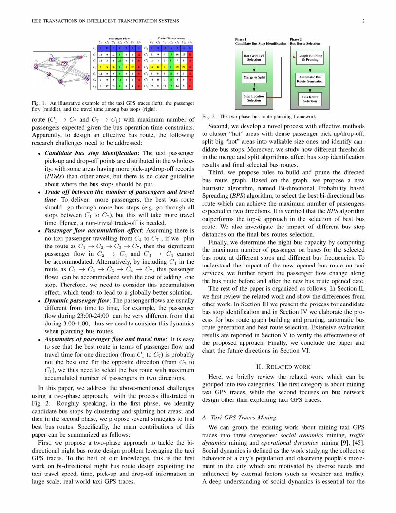
However, identifying the candidate bus stops from taxi GPSdata and enumerating the top-ranked bi-directional bus routesefficiently are not trivial and straight-forward. To the best ofour knowledge, there is still no work reported on this topic.For example, given the taxi GPS trajectories of night time fora certain time period, let us say that seven dense taxi pick-up/drop-off locations (i.e. C1 − C7) have been identified ascandidate bus stops as illustrated in Fig. 1, where C1 andC7 are the bus origin and destination, respectively, and thecorresponding passenger flow and travel time among stopsare shown in the right panel of Fig. 1. The objective of bi-directional bus route design is to find a bi-directional bus

IEEE TRANSACTIONS ON INTELLIGENT TRANSPORTATION SYSTEMS 2

C1

C2

C3

C4

C5

C6C7

C1 C2 C3 C4 C5 C6 C7

0 15 7 0 9 0 5

18 0 12 8 0 0 12

14 3 0 20 0 0 9

0 5 10 0 0 22 0

12 0 0 0 0 9 0

0 0 0 13 0 0 10

3 17 13 0 0 4 0

C1

C2

C3

C4

C5

C6

C7

C1 C2 C3 C4 C5 C6 C7

0 8 10 15 9 15 25

9 0 4 10 16 19 22

11 3 0 6 7 8 14

16 12 7 0 29 27 10

8 14 6 25 0 5 12

14 18 7 26 4 0 10

27 21 15 12 14 9 0

C1

C2

C3

C4

C5

C6

C7

Passenger Flow Travel Time(in minute)

Fig. 1. An illustrative example of the taxi GPS traces (left); the passengerflow (middle), and the travel time among bus stops (right).

route (C1 → C7 and C7 → C1) with maximum number ofpassengers expected given the bus operation time constraints.Apparently, to design an effective bus route, the followingresearch challenges need to be addressed:

• Candidate bus stop identification: The taxi passengerpick-up and drop-off points are distributed in the whole c-ity, with some areas having more pick-up/drop-off records(PDRs) than other areas, but there is no clear guidelineabout where the bus stops should be put.

• Trade off between the number of passengers and traveltime: To deliver more passengers, the best bus routeshould go through more bus stops (e.g. go through allstops between C1 to C7), but this will take more traveltime. Hence, a non-trivial trade-off is needed.

• Passenger flow accumulation effect: Assuming there isno taxi passenger travelling from C4 to C7 , if we planthe route as C1 → C2 → C3 → C7, then the significantpassenger flow in C2 → C4 and C3 → C4 cannotbe accommodated. Alternatively, by including C4 in theroute as C1 → C2 → C3 → C4 → C7, this passengerflows can be accommodated with the cost of adding onestop. Therefore, we need to consider this accumulationeffect, which tends to lead to a globally better solution.

• Dynamic passenger flow: The passenger flows are usuallydifferent from time to time, for example, the passengerflow during 23:00-24:00 can be very different from thatduring 3:00-4:00, thus we need to consider this dynamicswhen planning bus routes.

• Asymmetry of passenger flow and travel time: It is easyto see that the best route in terms of passenger flow andtravel time for one direction (from C1 to C7) is probablynot the best one for the opposite direction (from C7 toC1), we thus need to select the bus route with maximumaccumulated number of passengers in two directions.

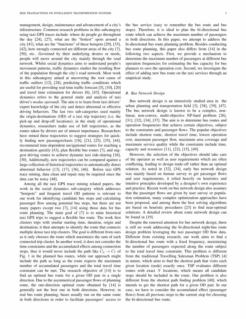
In this paper, we address the above-mentioned challengesusing a two-phase approach, with the process illustrated inFig. 2. Roughly speaking, in the first phase, we identifycandidate bus stops by clustering and splitting hot areas; andthen in the second phase, we propose several strategies to findbest bus routes. Specifically, the main contributions of thispaper can be summarized as follows:

First, we propose a two-phase approach to tackle the bi-directional night bus route design problem leveraging the taxiGPS traces. To the best of our knowledge, this is the firstwork on bi-directional night bus route design exploiting thetaxi travel speed, time, pick-up and drop-off information inlarge-scale, real-world taxi GPS traces.

Phase 1Candidate Bus Stop Identification

Phase 2Bus Route Selection

Hot Grid Cell Selection

Merge & Split

Stop Location Selection

Graph Building & Pruning

Automatic Bus Route Generation

Bus Route Selection

Fig. 2. The two-phase bus route planning framework.

Second, we develop a novel process with effective methodsto cluster “hot” areas with dense passenger pick-up/drop-off,split big “hot” areas into walkable size ones and identify can-didate bus stops. Moreover, we study how different thresholdsin the merge and split algorithms affect bus stop identificationresults and final selected bus routes.

Third, we propose rules to build and prune the directedbus route graph. Based on the graph, we propose a newheuristic algorithm, named Bi-directional Probability basedSpreading (BPS) algorithm, to select the best bi-directional busroute which can achieve the maximum number of passengersexpected in two directions. It is verified that the BPS algorithmoutperforms the top-k approach in the selection of best busroute. We also investigate the impact of different bus stopdistances on the final bus routes selection.

Finally, we determine the night bus capacity by computingthe maximum number of passenger on buses for the selectedbus route at different stops and different bus frequencies. Tounderstand the impact of the new opened bus route on taxiservices, we further report the passenger flow change alongthe bus route before and after the new bus route opened date.

The rest of the paper is organized as follows. In Section II,we first review the related work and show the differences fromother work. In Section III we present the process for candidatebus stop identification and in Section IV we elaborate the pro-cess for bus route graph building and pruning, automatic busroute generation and best route selection. Extensive evaluationresults are reported in Section V to verify the effectiveness ofthe proposed approach. Finally, we conclude the paper andchart the future directions in Section VI.

II. RELATED WORK

Here, we briefly review the related work which can begrouped into two categories. The first category is about miningtaxi GPS traces, while the second focuses on bus networkdesign other than exploiting taxi GPS traces.

A. Taxi GPS Traces Mining

We can group the existing work about mining taxi GPStraces into three categories: social dynamics mining, trafficdynamics mining and operational dynamics mining [9], [45].Social dynamics is defined as the work studying the collectivebehavior of a city’s population and observing people’s move-ment in the city which are motivated by diverse needs andinfluenced by external factors (such as weather and traffic).A deep understanding of social dynamics is essential for the

IEEE TRANSACTIONS ON INTELLIGENT TRANSPORTATION SYSTEMS 3

management, design, maintenance and advancement of a city’sinfrastructure. Common research problems in this subcategoryusing taxi GPS traces include: where do people go throughoutthe day [24], [27], what are the “hottest” spots around acity [41], what are the “functions” of these hotspots [29], [33],[42], how strongly connected are different areas of the city [7],[50], etc.. Governed by their underlying desires or needs,people will move around the city mainly through the roadnetwork. Whilst social dynamics aims to understand people’smovement patterns, traffic dynamics studies the resulting flowof the population through the city’s road network. Most workin this subcategory aimed at uncovering the root cause oftraffic outliers [12], [28], predicting traffic conditions whichare useful for providing real-time traffic forecast [5], [10], [20]and travel time estimation for drivers [6], [43]. Operationaldynamics refers to the general study and analysis of taxidriver’s modus operandi. The aim is to learn from taxi drivers’expert knowledge of the city and detect abnormal or effectivedriving behaviors. The last two sub-categories used mainlythe origin-destinations (OD) of a taxi trip trajectory (i.e. thepick-up and drop-off locations); in the study of operationaldynamics, researchers make use of full trajectories, as theroutes taken by drivers are of utmost importance. Researchershave mined these trajectories to suggest strategies for quick-ly finding new passengers/taxis [18], [21], [25], [35], [44],recommend time-dependent navigational routes for reaching adestination quickly [43], plan flexible bus routes [7], and sug-gest driving routes to achieve dynamic taxi ride-sharing [16],[30]. Additionally, new trajectories can be compared against alarge collection of historical trajectories to automatically detectabnormal behavior [13], [17], [36], [46]. Before taxi GPStrace mining, data clean and repair may be required since thedata can be noisy [48].

Among all the taxi GPS trace mining related papers, thework in the social dynamics sub-category which addresses“hotspots” and frequent travel OD patterns is relevant toour work for identifying candidate bus stops and calculatingpassenger flow among potential bus stops, but there are notmany papers except two [7], [14] using those data for busroute planning. The main goal of [7] is to mine historicaltaxi GPS trips to suggest a flexible bus route. The work firstclusters trips with similar starting time, duration, origin anddestination; it then attempts to identify the route that connectsmultiple dense taxi trip clusters. The goal is different from oursas it only chooses the route which maximizes the sum of eachconnected trip cluster. In another word, it does not consider thetime constraints and the accumulated effects among connectionstops, thus it would never include the path like C4 → C7 ofFig. 1 in the planned bus routes, while our approach mightinclude the path as long as the route expects the maximumnumber of accumulated passengers and the total travel timeconstraint can be met. The research objective of [14] is tofind an optimal bus route for a given OD pair in a singledirection. Due to the asymmetrical passenger flows of planningroute, the one-direction optimal route obtained by [14] isgenerally not the best one in both directions. However, inreal bus route planning, buses usually run on the same routein both directions in order to facilitate passengers’ access to

the bus service (easy to remember the bus route and busstops). Therefore, it is ideal to plan the bi-directional busroute which can achieve the maximum number of passengersin both directions. In this paper, we attempt to address thebi-directional bus route planning problem. Besides conductingbus route planning, this paper also differs from [14] in thefollowing two aspects. First, we provide a mechanism todetermine the maximum number of passengers at different busoperation frequencies for estimating the bus capacity for busplanners to save the operation cost. Second, we investigate theeffect of adding new bus route on the taxi services through anempirical study.

B. Bus Network Design

Bus network design is an intensively studied area in theurban planning and transportation field [3], [38], [39], [47].The bus network design is known to be a complex, non-linear, non-convex, multi-objective NP-hard problem [26],[31], [32], [34], [37]. The aim is to determine bus routes andoperation frequencies that achieve certain objectives, subjectto the constraints and passenger flows. The popular objectivesinclude shortest route, shortest travel time, lowest operationcost, maximum passenger flow, maximum area coverage andmaximum service quality while the constraints include time,capacity and resources [11], [22], [15], [49].

However, the selection of the objectives should take careof the operator as well as user requirements which are oftenconflicting, leading to design trade-off rather than an optimalsolution. As noted in [32], [34], early bus network designwas mainly based on human survey to get passenger flowsand user requirements, it relied heavily on heuristics andintuitive principles developed by a designer’s own experienceand practice. Recent work on bus network design also assumesthat the passenger flows are given by user survey or popula-tion estimation, many complex optimization approaches havebeen proposed, and among them the best solving algorithmsare based on heuristic procedures [23] to find near-optimalsolutions. A detailed review about route network design canbe found in [19].

Despite the renewed attention for bus network design, thereis still no work addressing the bi-directional night-bus routedesign problem leveraging the taxi passenger OD flow data.Different from existing research, our work aims to find abi-directional bus route with a fixed frequency, maximizingthe number of passengers expected along the route subjectto the total travel time constraint. This problem is differentfrom the traditional Travelling Salesman Problem (TSP) [4]in nature, which aims to find the shortest path that visits eachgiven location (node) exactly once. TSP evaluates differentroutes with exact N locations, which means all candidatestops should be included in the route. Our problem is alsodifferent from the shortest path finding problem [40], whichintends to get the shortest path for a given OD pair. In ourcase, we have to consider the accumulated effect (passengerflows) from all previous stops to the current stop for choosingthe bi-directional bus route.

IEEE TRANSACTIONS ON INTELLIGENT TRANSPORTATION SYSTEMS 4

III. CANDIDATE BUS STOP IDENTIFICATION

In the proposed two-phase bus route planning framework,the objective of the phase one is to identify candidate busstops by exploiting the taxi PDRs. In this section, we describeour proposed process for identifying candidate bus stops. Asshown in Fig. 2, the whole process consists of three steps:(1) Divide the whole city into small equal-sized grid cells,mark those “hot” grid cells with high taxi passenger PDRs forfurther processing; (2) Merge the adjacent “hot” grid cells toform “hot” areas, divide each big area into “walkable size”cluster; (3) Choose one grid cell as the candidate bus stoplocation in each walkable size “hot” cluster, by assuming thatpassengers from the same cluster would easily walk to the stopto take bus.

A. Hot Grid Cells and City Partitions

In this work, we first divide the city into equal-sized gridcells, with each cell about 10m× 10m in size. In such a way,the whole city is partitioned into 5000 × 2500 cells in total.Out of all the grid cells, over 95% of them contain no taxipassenger PDRs as they are either lakes, mountains, buildings,and highways that cannot be reached by taxis, or suburb areasthat people seldom travel to. Only 0.11% of the grid cells havemore than 0.2 PDRs per hour on average if we only count thePDRs in late night. And we name these grid cells as “hot”ones.

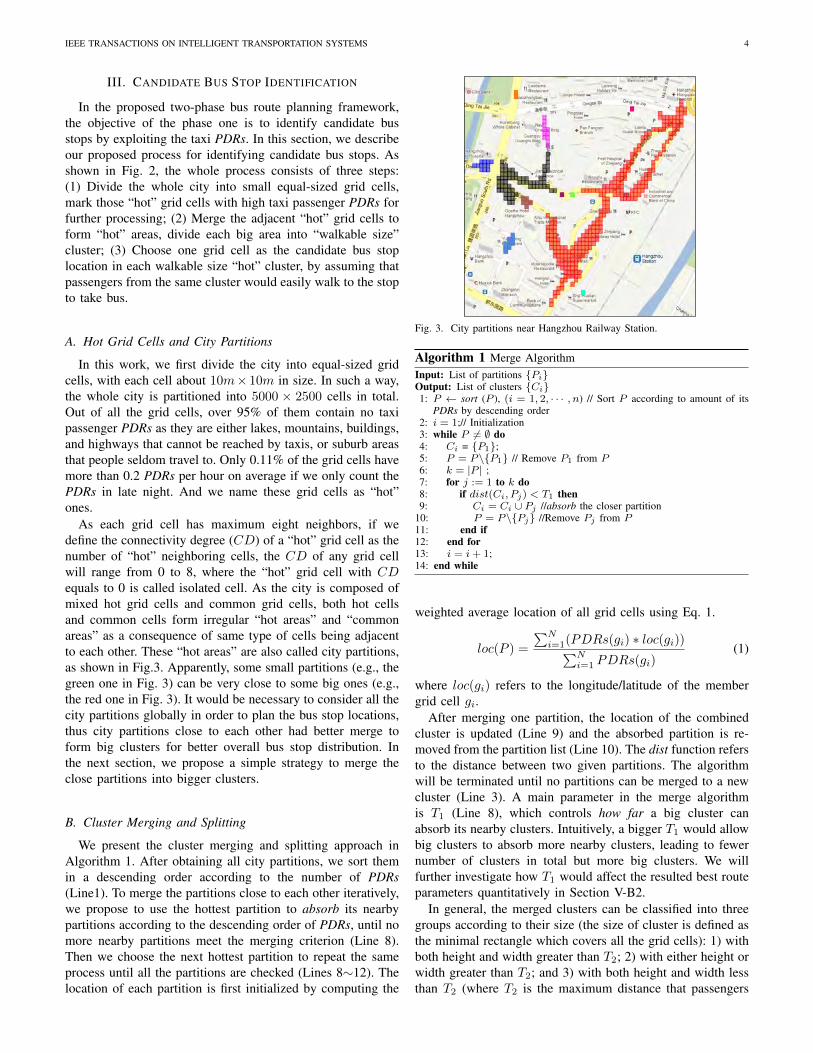
As each grid cell has maximum eight neighbors, if wedefine the connectivity degree (CD) of a “hot” grid cell as thenumber of “hot” neighboring cells, the CD of any grid cellwill range from 0 to 8, where the “hot” grid cell with CDequals to 0 is called isolated cell. As the city is composed ofmixed hot grid cells and common grid cells, both hot cellsand common cells form irregular “hot areas” and “commonareas” as a consequence of same type of cells being adjacentto each other. These “hot areas” are also called city partitions,as shown in Fig.3. Apparently, some small partitions (e.g., thegreen one in Fig. 3) can be very close to some big ones (e.g.,the red one in Fig. 3). It would be necessary to consider all thecity partitions globally in order to plan the bus stop locations,thus city partitions close to each other had better merge toform big clusters for better overall bus stop distribution. Inthe next section, we propose a simple strategy to merge theclose partitions into bigger clusters.

B. Cluster Merging and Splitting

We present the cluster merging and splitting approach inAlgorithm 1. After obtaining all city partitions, we sort themin a descending order according to the number of PDRs(Line1). To merge the partitions close to each other iteratively,we propose to use the hottest partition to absorb its nearbypartitions according to the descending order of PDRs, until nomore nearby partitions meet the merging criterion (Line 8).Then we choose the next hottest partition to repeat the sameprocess until all the partitions are checked (Lines 8∼12). Thelocation of each partition is first initialized by computing the

Fig. 3. City partitions near Hangzhou Railway Station.

Algorithm 1 Merge AlgorithmInput: List of partitions {Pi}Output: List of clusters {Ci}1: P ← sort (P ), (i = 1, 2, · · · , n) // Sort P according to amount of its

PDRs by descending order2: i = 1;// Initialization3: while P 6= ∅ do4: Ci = {P1};5: P = P\{P1} // Remove P1 from P6: k = |P | ;7: for j := 1 to k do8: if dist(Ci, Pj) < T1 then9: Ci = Ci ∪ Pj //absorb the closer partition

10: P = P\{Pj} //Remove Pj from P11: end if12: end for13: i = i+ 1;14: end while

weighted average location of all grid cells using Eq. 1.

loc(P ) =

∑Ni=1(PDRs(gi) ∗ loc(gi))∑N

i=1 PDRs(gi)(1)

where loc(gi) refers to the longitude/latitude of the membergrid cell gi.

After merging one partition, the location of the combinedcluster is updated (Line 9) and the absorbed partition is re-moved from the partition list (Line 10). The dist function refersto the distance between two given partitions. The algorithmwill be terminated until no partitions can be merged to a newcluster (Line 3). A main parameter in the merge algorithmis T1 (Line 8), which controls how far a big cluster canabsorb its nearby clusters. Intuitively, a bigger T1 would allowbig clusters to absorb more nearby clusters, leading to fewernumber of clusters in total but more big clusters. We willfurther investigate how T1 would affect the resulted best routeparameters quantitatively in Section V-B2.

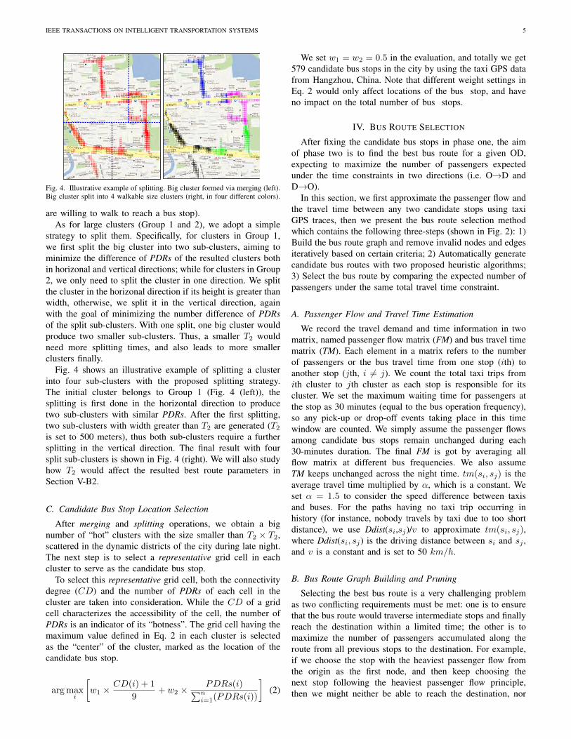
In general, the merged clusters can be classified into threegroups according to their size (the size of cluster is defined asthe minimal rectangle which covers all the grid cells): 1) withboth height and width greater than T2; 2) with either height orwidth greater than T2; and 3) with both height and width lessthan T2 (where T2 is the maximum distance that passengers

IEEE TRANSACTIONS ON INTELLIGENT TRANSPORTATION SYSTEMS 5

Fig. 4. Illustrative example of splitting. Big cluster formed via merging (left).Big cluster split into 4 walkable size clusters (right, in four different colors).

are willing to walk to reach a bus stop).As for large clusters (Group 1 and 2), we adopt a simple

strategy to split them. Specifically, for clusters in Group 1,we first split the big cluster into two sub-clusters, aiming tominimize the difference of PDRs of the resulted clusters bothin horizonal and vertical directions; while for clusters in Group2, we only need to split the cluster in one direction. We splitthe cluster in the horizonal direction if its height is greater thanwidth, otherwise, we split it in the vertical direction, againwith the goal of minimizing the number difference of PDRsof the split sub-clusters. With one split, one big cluster wouldproduce two smaller sub-clusters. Thus, a smaller T2 wouldneed more splitting times, and also leads to more smallerclusters finally.

Fig. 4 shows an illustrative example of splitting a clusterinto four sub-clusters with the proposed splitting strategy.The initial cluster belongs to Group 1 (Fig. 4 (left)), thesplitting is first done in the horizontal direction to producetwo sub-clusters with similar PDRs. After the first splitting,two sub-clusters with width greater than T2 are generated (T2is set to 500 meters), thus both sub-clusters require a furthersplitting in the vertical direction. The final result with foursplit sub-clusters is shown in Fig. 4 (right). We will also studyhow T2 would affect the resulted best route parameters inSection V-B2.

C. Candidate Bus Stop Location Selection

After merging and splitting operations, we obtain a bignumber of “hot” clusters with the size smaller than T2 × T2,scattered in the dynamic districts of the city during late night.The next step is to select a representative grid cell in eachcluster to serve as the candidate bus stop.

To select this representative grid cell, both the connectivitydegree (CD) and the number of PDRs of each cell in thecluster are taken into consideration. While the CD of a gridcell characterizes the accessibility of the cell, the number ofPDRs is an indicator of its “hotness”. The grid cell having themaximum value defined in Eq. 2 in each cluster is selectedas the “center” of the cluster, marked as the location of thecandidate bus stop.

arg maxi

[w1 ×

CD(i) + 1

9+ w2 ×

PDRs(i)∑ni=1(PDRs(i))

](2)

We set w1 = w2 = 0.5 in the evaluation, and totally we get579 candidate bus stops in the city by using the taxi GPS datafrom Hangzhou, China. Note that different weight settings inEq. 2 would only affect locations of the bus stop, and haveno impact on the total number of bus stops.

IV. BUS ROUTE SELECTION

After fixing the candidate bus stops in phase one, the aimof phase two is to find the best bus route for a given OD,expecting to maximize the number of passengers expectedunder the time constraints in two directions (i.e. O→D andD→O).

In this section, we first approximate the passenger flow andthe travel time between any two candidate stops using taxiGPS traces, then we present the bus route selection methodwhich contains the following three-steps (shown in Fig. 2): 1)Build the bus route graph and remove invalid nodes and edgesiteratively based on certain criteria; 2) Automatically generatecandidate bus routes with two proposed heuristic algorithms;3) Select the bus route by comparing the expected number ofpassengers under the same total travel time constraint.

A. Passenger Flow and Travel Time Estimation

We record the travel demand and time information in twomatrix, named passenger flow matrix (FM) and bus travel timematrix (TM). Each element in a matrix refers to the numberof passengers or the bus travel time from one stop (ith) toanother stop (jth, i 6= j). We count the total taxi trips fromith cluster to jth cluster as each stop is responsible for itscluster. We set the maximum waiting time for passengers atthe stop as 30 minutes (equal to the bus operation frequency),so any pick-up or drop-off events taking place in this timewindow are counted. We simply assume the passenger flowsamong candidate bus stops remain unchanged during each30-minutes duration. The final FM is got by averaging allflow matrix at different bus frequencies. We also assumeTM keeps unchanged across the night time. tm(si, sj) is theaverage travel time multiplied by α, which is a constant. Weset α = 1.5 to consider the speed difference between taxisand buses. For the paths having no taxi trip occurring inhistory (for instance, nobody travels by taxi due to too shortdistance), we use Ddist(si,sj)/v to approximate tm(si, sj),where Ddist(si, sj) is the driving distance between si and sj ,and v is a constant and is set to 50 km/h.

B. Bus Route Graph Building and Pruning

Selecting the best bus route is a very challenging problemas two conflicting requirements must be met: one is to ensurethat the bus route would traverse intermediate stops and finallyreach the destination within a limited time; the other is tomaximize the number of passengers accumulated along theroute from all previous stops to the destination. For example,if we choose the stop with the heaviest passenger flow fromthe origin as the first node, and then keep choosing thenext stop following the heaviest passenger flow principle,then we might neither be able to reach the destination, nor

IEEE TRANSACTIONS ON INTELLIGENT TRANSPORTATION SYSTEMS 6

O

D

21

3

X

Y

Xnew

Ynew

✓

O

D

3

1

2

4

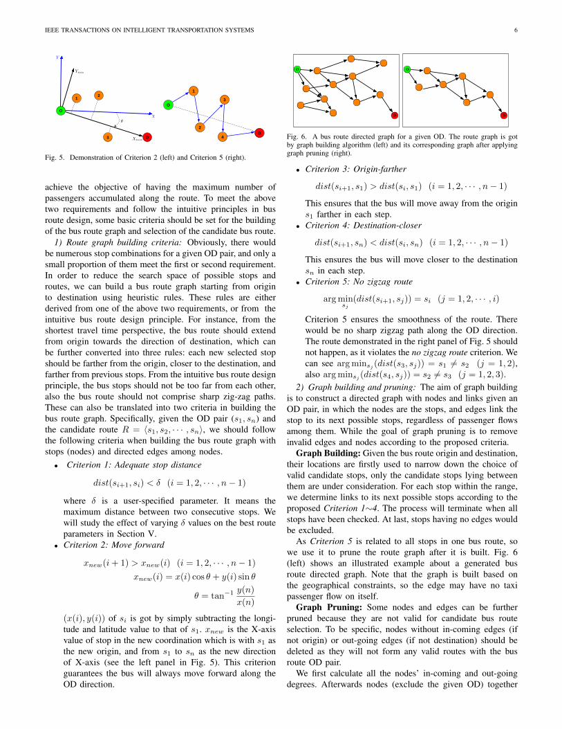
Fig. 5. Demonstration of Criterion 2 (left) and Criterion 5 (right).

achieve the objective of having the maximum number ofpassengers accumulated along the route. To meet the abovetwo requirements and follow the intuitive principles in busroute design, some basic criteria should be set for the buildingof the bus route graph and selection of the candidate bus route.

1) Route graph building criteria: Obviously, there wouldbe numerous stop combinations for a given OD pair, and only asmall proportion of them meet the first or second requirement.In order to reduce the search space of possible stops androutes, we can build a bus route graph starting from originto destination using heuristic rules. These rules are eitherderived from one of the above two requirements, or from theintuitive bus route design principle. For instance, from theshortest travel time perspective, the bus route should extendfrom origin towards the direction of destination, which canbe further converted into three rules: each new selected stopshould be farther from the origin, closer to the destination, andfarther from previous stops. From the intuitive bus route designprinciple, the bus stops should not be too far from each other,also the bus route should not comprise sharp zig-zag paths.These can also be translated into two criteria in building thebus route graph. Specifically, given the OD pair (s1, sn) andthe candidate route R = 〈s1, s2, · · · , sn〉, we should followthe following criteria when building the bus route graph withstops (nodes) and directed edges among nodes.• Criterion 1: Adequate stop distance

dist(si+1, si) < δ (i = 1, 2, · · · , n− 1)

where δ is a user-specified parameter. It means themaximum distance between two consecutive stops. Wewill study the effect of varying δ values on the best routeparameters in Section V.

• Criterion 2: Move forward

xnew(i+ 1) > xnew(i) (i = 1, 2, · · · , n− 1)

xnew(i) = x(i) cos θ + y(i) sin θ

θ = tan−1y(n)

x(n)

(x(i), y(i)) of si is got by simply subtracting the longi-tude and latitude value to that of s1. xnew is the X-axisvalue of stop in the new coordination which is with s1 asthe new origin, and from s1 to sn as the new directionof X-axis (see the left panel in Fig. 5). This criterionguarantees the bus will always move forward along theOD direction.

O

D

O

D

Fig. 6. A bus route directed graph for a given OD. The route graph is gotby graph building algorithm (left) and its corresponding graph after applyinggraph pruning (right).

• Criterion 3: Origin-farther

dist(si+1, s1) > dist(si, s1) (i = 1, 2, · · · , n− 1)

This ensures that the bus will move away from the origins1 farther in each step.

• Criterion 4: Destination-closer

dist(si+1, sn) < dist(si, sn) (i = 1, 2, · · · , n− 1)

This ensures the bus will move closer to the destinationsn in each step.

• Criterion 5: No zigzag route

arg minsj

(dist(si+1, sj)) = si (j = 1, 2, · · · , i)

Criterion 5 ensures the smoothness of the route. Therewould be no sharp zigzag path along the OD direction.The route demonstrated in the right panel of Fig. 5 shouldnot happen, as it violates the no zigzag route criterion. Wecan see arg minsj (dist(s3, sj)) = s1 6= s2 (j = 1, 2),also arg minsj (dist(s4, sj)) = s2 6= s3 (j = 1, 2, 3).

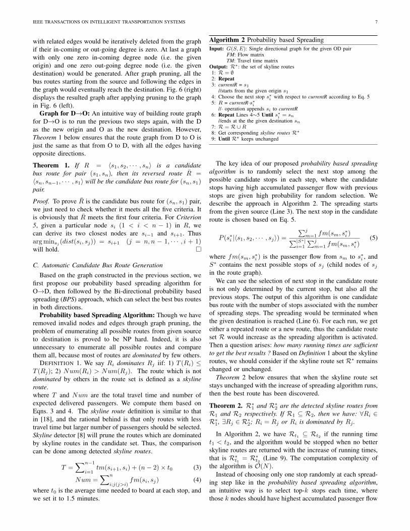
2) Graph building and pruning: The aim of graph buildingis to construct a directed graph with nodes and links given anOD pair, in which the nodes are the stops, and edges link thestop to its next possible stops, regardless of passenger flowsamong them. While the goal of graph pruning is to removeinvalid edges and nodes according to the proposed criteria.

Graph Building: Given the bus route origin and destination,their locations are firstly used to narrow down the choice ofvalid candidate stops, only the candidate stops lying betweenthem are under consideration. For each stop within the range,we determine links to its next possible stops according to theproposed Criterion 1∼4. The process will terminate when allstops have been checked. At last, stops having no edges wouldbe excluded.

As Criterion 5 is related to all stops in one bus route, sowe use it to prune the route graph after it is built. Fig. 6(left) shows an illustrated example about a generated busroute directed graph. Note that the graph is built based onthe geographical constraints, so the edge may have no taxipassenger flow on itself.

Graph Pruning: Some nodes and edges can be furtherpruned because they are not valid for candidate bus routeselection. To be specific, nodes without in-coming edges (ifnot origin) or out-going edges (if not destination) should bedeleted as they will not form any valid routes with the busroute OD pair.

We first calculate all the nodes’ in-coming and out-goingdegrees. Afterwards nodes (exclude the given OD) together

IEEE TRANSACTIONS ON INTELLIGENT TRANSPORTATION SYSTEMS 7

with related edges would be iteratively deleted from the graphif their in-coming or out-going degree is zero. At last a graphwith only one zero in-coming degree node (i.e. the givenorigin) and one zero out-going degree node (i.e. the givendestination) would be generated. After graph pruning, all thebus routes starting from the source and following the edges inthe graph would eventually reach the destination. Fig. 6 (right)displays the resulted graph after applying pruning to the graphin Fig. 6 (left).

Graph for D→O: An intuitive way of building route graphfor D→O is to run the previous two steps again, with the Das the new origin and O as the new destination. However,Theorem 1 below ensures that the route graph from D to O isjust the same as that from O to D, with all the edges havingopposite directions.

Theorem 1. If R = 〈s1, s2, · · · , sn〉 is a candidatebus route for pair (s1, sn), then its reversed route R̄ =〈sn, sn−1, · · · , s1〉 will be the candidate bus route for (sn, s1)pair.

Proof. To prove R̄ is the candidate bus route for (sn, s1) pair,we just need to check whether it meets all the five criteria. Itis obviously that R̄ meets the first four criteria. For Criterion5, given a particular node si (1 < i < n − 1) in R, wecan derive its two closest nodes are si−1 and si+1. Thusarg minsj (dist(si, sj)) = si+1 (j = n, n − 1, · · · , i + 1)will hold.

C. Automatic Candidate Bus Route GenerationBased on the graph constructed in the previous section, we

first propose our probability based spreading algorithm forO→D, then followed by the Bi-directional probability basedspreading (BPS) approach, which can select the best bus routesin both directions.

Probability based Spreading Algorithm: Though we haveremoved invalid nodes and edges through graph pruning, theproblem of enumerating all possible routes from given sourceto destination is proved to be NP hard. Indeed, it is alsounnecessary to enumerate all possible routes and comparethem all, because most of routes are dominated by few others.

DEFINITION 1. We say Ri dominates Rj iif: 1) T (Ri) ≤T (Rj); 2) Num(Ri) > Num(Rj). The route which is notdominated by others in the route set is defined as a skylineroute.where T and Num are the total travel time and number ofexpected delivered passengers. We compute them based onEqns. 3 and 4. The skyline route definition is similar to thatin [18], and the rational behind is that only routes with lesstravel time but larger number of passengers should be selected.Skyline detector [8] will prune the routes which are dominatedby skyline routes in the candidate set. Thus, the comparisoncan be done among detected skyline routes.

T =∑n−1

i=1tm(si+1, si) + (n− 2)× t0 (3)

Num =∑n

i;j(j>i)fm(si, sj) (4)

where t0 is the average time needed to board at each stop, andwe set it to 1.5 minutes.

Algorithm 2 Probability based SpreadingInput: G(S,E): Single directional graph for the given OD pair

FM: Flow matrixTM: Travel time matrix

Output: R∗: the set of skyline routes1: R = ∅2: Repeat3: currentR = s1

//starts from the given origin s14: Choose the next stop s∗i with respect to currentR according to Eq. 55: R = currentR·s∗i

//· operation appends si to currentR6: Repeat Lines 4∼5 Until s∗i = sn

//ends at the the given destination sn7: R = R∪R8: Get corresponding skyline routes R∗9: Until R∗ keeps unchanged

The key idea of our proposed probability based spreadingalgorithm is to randomly select the next stop among thepossible candidate stops in each step, where the candidatestops having high accumulated passenger flow with previousstops are given high probability for random selection. Wedescribe the approach in Algorithm 2. The spreading startsfrom the given source (Line 3). The next stop in the candidateroute is chosen based on Eq. 5.

P (s∗i |〈s1, s2, · · · , sj〉) =

∑jm=1 fm(sm, s

∗i )∑|S∗|

i=1

∑jm=1 fm(sm, s∗i )

(5)

where fm(sm, s∗i ) is the passenger flow from sm to s∗i , and

S∗ contains the next possible stops of sj (child nodes of sjin the route graph).

We can see the selection of next stop in the candidate routeis not only determined by the current stop, but also all theprevious stops. The output of this algorithm is one candidatebus route with the number of stops associated with the numberof spreading steps. The spreading would be terminated whenthe given destination is reached (Line 6). For each run, we geteither a repeated route or a new route, thus the candidate routeset R would increase as the spreading algorithm is activated.Then a question arises: how many running times are sufficientto get the best results ? Based on Definition 1 about the skylineroutes, we should consider if the skyline route set R∗ remainschanged or unchanged.

Theorem 2 below ensures that when the skyline route setstays unchanged with the increase of spreading algorithm runs,then the best route has been discovered.

Theorem 2. R∗1 and R∗2 are the detected skyline routes fromR1 and R2 respectively. If R1 ⊆ R2, then we have: ∀Ri ∈R∗1, ∃Rj ∈ R∗2; Ri = Rj or Ri is dominated by Rj .

In Algorithm 2, we have Rt1 ⊆ Rt2 if the running timet1 < t2, and the algorithm would be stopped when no betterskyline routes are returned with the increase of running times,that is R∗t1 = R∗t2 (Line 9). The computation complexity ofthe algorithm is O(N).

Instead of choosing only one stop randomly at each spread-ing step like in the probability based spreading algorithm,an intuitive way is to select top-k stops each time, wherethose k nodes should have highest accumulated passenger flow

IEEE TRANSACTIONS ON INTELLIGENT TRANSPORTATION SYSTEMS 8

Algorithm 3 BPS AlgorithmInput: GO→D(S,E): Graph for O → D

GD→O(S,E): Graph for D → OFM: Flow matrixTM: Travel time matrix

Output: R∗: the set of skyline routes1: R = ∅2: Repeat3: Run Line 2∼6 in Algorithm 2 for GO→D(S,E), and the output isRO→D

4: Run Line 2∼6 in Algorithm 2 for GD→O(S,E), and the output isRD→O

5: R = R∪RO→D ∪RD→O

6: Get corresponding skyline routes R∗7: Until R∗ keeps unchanged

with previous stops. In such a way, the first step selects top-k nodes, thus leading to k routes from the origin to thosenodes. In the second step, each k nodes would select anothertop-k nodes, thus the total candidate routes would be k2.Assume that n steps are needed to the destination, then thetotal candidate routes generated would be kn in the end. Thus,the computation complexity of this algorithm is O(kn), whichgrows exponentially with the spreading step (n). We use thistop-k spreading method as the baseline.

Bi-directional Probability based Spreading (BPS) Algo-rithm: In practice, for a particular bus line, buses can run onthe same route in both directions. Algorithm 2 can get the bestbus route in one direction (e.g. from ZJU to Railway Station),however, it cannot guarantee the same route in the oppositedirection (i.e. from Railway Station to ZJU) would still expectthe maximum number of passengers, as the passenger flows intwo directions of the route are generally asymmetrical. To geta bus route which has overall maximum expected number ofpassengers in both directions, we propose the BPS algorithm,whose basic idea is to run the probability based spreadingalgorithm in both directions so that we generate one candidate“optimal” route in each direction, and the best route is selectedby evaluating all the candidate routes in two directions.

We illustrate the procedure in Algorithm 3. The key ideabehind is to run Algorithm 2 in both directions (Line 3∼4),and generate one candidate route for each direction at eachrun (Line 5). The skyline routes are selected based on thetotal travel time and expected number of passengers in bothdirections of each candidate route (Line 6), and the selectionprocess terminates also when no more better skyline routescan be generated (Line 7).D. Bus Route Selection

Given the bus operation frequency (once every 30 minutes),the total travel time constraint, and the taxi passenger flowfrom 21:30 to 5:30, we obtain the candidate bus routes fora given OD pair using the two different heuristic spreadingalgorithms, and the skyline route which achieves the maxi-mum expected number of passengers will be selected as theoperating route.

With the planned bus route consisting of the selected busstops, the next step is to find a physical bus route in the realsetting, which consists of road segments corresponding to theplanned route. The selection of each road segment is doneby following the dense and fine trajectories of taxis if they

TABLE IDETAILED INFORMATION ABOUT STUDIED OD PAIRS.

OD Pairs Distance (km) Number of Stops

1 ZJU - Railway 5.70 1042 Railway - East Railway 5.86 753 East Railway - ZJU 8.80 144

allow buses to operate; Otherwise similar bus routes near theplanned ones can be adopted as a refined solution.

V. EXPERIMENTAL EVALUATION

In this section, we validate the proposed approach with alarge-scale real-world taxi GPS dataset which is generatedfrom 7,600 taxis in a large city in China (Hangzhou) inone month, with more than 1.57 million of night passenger-delivering trips. All the experiments are run in Matlab on anIntel Xeon W3500 PC with 12-GB RAM running Windows 7.

A. Evaluation on Bus Stops

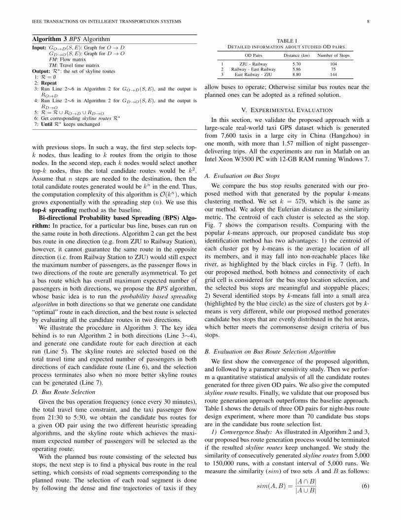
We compare the bus stop results generated with our pro-posed method with that generated by the popular k-meansclustering method. We set k = 579, which is the same asour method. We adopt the Eulerian distance as the similaritymetric. The centroid of each cluster is selected as the stop.Fig. 7 shows the comparison results. Comparing with thepopular k-means approach, our proposed candidate bus stopidentification method has two advantages: 1) the centroid ofeach cluster got by k-means is the average location of allits members, and it may fall into non-reachable places likeriver, as highlighted by the black circles in Fig. 7 (left). Inour proposed method, both hotness and connectivity of eachgrid cell is considered for the bus stop location selection, andthe selected bus stops are meaningful and stoppable places;2) Several identified stops by k-means fall into a small area(highlighted by the blue circle) as the size of clusters got by k-means is very different, while our proposed method generatescandidate bus stops that are evenly distributed in the hot areas,which better meets the commonsense design criteria of busstops.

B. Evaluation on Bus Route Selection Algorithm

We first show the convergence of the proposed algorithm,and followed by a parameter sensitivity study. Then we perfor-m a quantitative statistical analysis of all the candidate routesgenerated for three given OD pairs. We also give the computedskyline route results. Finally, we validate that our proposed busroute generation approach outperforms the baseline approach.Table I shows the details of three OD pairs for night-bus routedesign experiment, where more than 70 candidate bus stopsare in the candidate bus route selection list.

1) Convergence Study: As illustrated in Algorithm 2 and 3,our proposed bus route generation process would be terminatedif the resulted skyline routes keep unchanged. We study thesimilarity of consecutively generated skyline routes from 5,000to 150,000 runs, with a constant interval of 5,000 runs. Wemeasure the similarity (sim) of two sets A and B as follows:

sim(A,B) =|A ∩B||A ∪B|

(6)

IEEE TRANSACTIONS ON INTELLIGENT TRANSPORTATION SYSTEMS 9

Fig. 7. Comparison results with k-means (best viewed in the digital version). Results got by k-means (left) and results got by our method (right).

0.5 1 1.5 2 2.5x 105

0

0.2

0.4

0.6

0.8

1

Sim

ilari

ty

Number of Runs

0.5 1 1.5 2 2.5x 105

0

300

600

900

1200

1500

1800

2100

2400

2700

3000

Tim

e C

ost (

s)

0.5 1 1.5 2 2.5x 105

0

300

600

900

1200

1500

1800

2100

2400

2700

3000

Tim

e C

ost (

s)

0.5 1 1.5 2 2.5x 105

0

300

600

900

1200

1500

1800

2100

2400

2700

3000

Tim

e C

ost (

s)

Fig. 8. Convergence study of the proposed BPS algorithm.

The similarity results of the consecutively generated skylineroutes with a 5,000 run interval are shown in Fig. 8, and thetime cost is put in the diagram as well. In this study, we cansee that sim values gradually reach 1 with the increase ofruns for all three OD pairs, meaning that in all three casesthe best bus route converges to one. Also the time cost isalmost linearly increased with the number of runs, suggestingthat the spreading time cost at each run is almost constant.It is also noted that the three curves for three OD pairs havedifferent slopes, the reason is probably because the bus routescorresponding to different ODs have different lengths andvaried number of candidate bus stops, thus the spreading timeand candidate bus stop selection time should be also different.

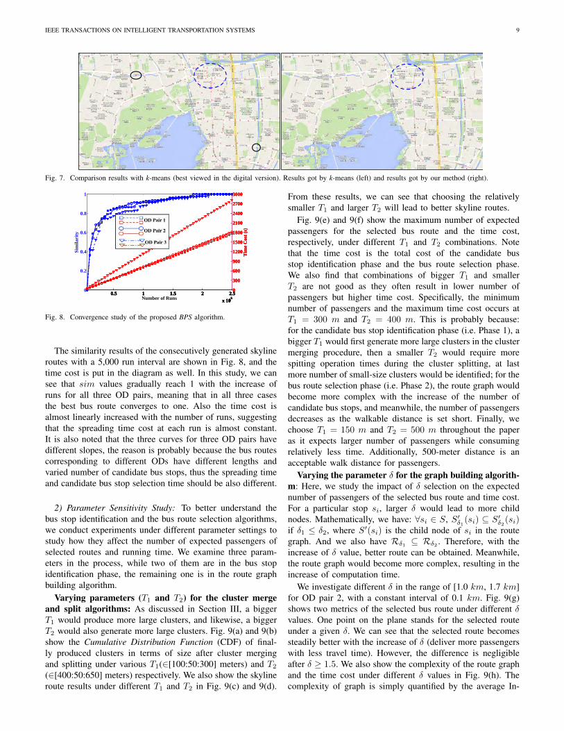
2) Parameter Sensitivity Study: To better understand thebus stop identification and the bus route selection algorithms,we conduct experiments under different parameter settings tostudy how they affect the number of expected passengers ofselected routes and running time. We examine three param-eters in the process, while two of them are in the bus stopidentification phase, the remaining one is in the route graphbuilding algorithm.

Varying parameters (T1 and T2) for the cluster mergeand split algorithms: As discussed in Section III, a biggerT1 would produce more large clusters, and likewise, a biggerT2 would also generate more large clusters. Fig. 9(a) and 9(b)show the Cumulative Distribution Function (CDF) of final-ly produced clusters in terms of size after cluster mergingand splitting under various T1(∈[100:50:300] meters) and T2(∈[400:50:650] meters) respectively. We also show the skylineroute results under different T1 and T2 in Fig. 9(c) and 9(d).

From these results, we can see that choosing the relativelysmaller T1 and larger T2 will lead to better skyline routes.

Fig. 9(e) and 9(f) show the maximum number of expectedpassengers for the selected bus route and the time cost,respectively, under different T1 and T2 combinations. Notethat the time cost is the total cost of the candidate busstop identification phase and the bus route selection phase.We also find that combinations of bigger T1 and smallerT2 are not good as they often result in lower number ofpassengers but higher time cost. Specifically, the minimumnumber of passengers and the maximum time cost occurs atT1 = 300 m and T2 = 400 m. This is probably because:for the candidate bus stop identification phase (i.e. Phase 1), abigger T1 would first generate more large clusters in the clustermerging procedure, then a smaller T2 would require morespitting operation times during the cluster splitting, at lastmore number of small-size clusters would be identified; for thebus route selection phase (i.e. Phase 2), the route graph wouldbecome more complex with the increase of the number ofcandidate bus stops, and meanwhile, the number of passengersdecreases as the walkable distance is set short. Finally, wechoose T1 = 150 m and T2 = 500 m throughout the paperas it expects larger number of passengers while consumingrelatively less time. Additionally, 500-meter distance is anacceptable walk distance for passengers.

Varying the parameter δ for the graph building algorith-m: Here, we study the impact of δ selection on the expectednumber of passengers of the selected bus route and time cost.For a particular stop si, larger δ would lead to more childnodes. Mathematically, we have: ∀si ∈ S, S′δ1(si) ⊆ S′δ2(si)if δ1 ≤ δ2, where S′(si) is the child node of si in the routegraph. And we also have Rδ1 ⊆ Rδ2 . Therefore, with theincrease of δ value, better route can be obtained. Meanwhile,the route graph would become more complex, resulting in theincrease of computation time.

We investigate different δ in the range of [1.0 km, 1.7 km]for OD pair 2, with a constant interval of 0.1 km. Fig. 9(g)shows two metrics of the selected bus route under different δvalues. One point on the plane stands for the selected routeunder a given δ. We can see that the selected route becomessteadily better with the increase of δ (deliver more passengerswith less travel time). However, the difference is negligibleafter δ ≥ 1.5. We also show the complexity of the route graphand the time cost under different δ values in Fig. 9(h). Thecomplexity of graph is simply quantified by the average In-

IEEE TRANSACTIONS ON INTELLIGENT TRANSPORTATION SYSTEMS 10

4 5 6 7 8 9 10 11 12 13 14 15 16 17 18 19 20 21 220

5

10

15

20

25

30

35

40

Number of Stops

Perc

enta

ges(

%)

OD Pair 1OD Pair 2OD Pair 3

Fig. 10. The number of stops of candidate route stops statistics for 3 ODpairs.

OD Pair 1

OD Pair 2

OD Pair 3

5 6 7 8 9 10 11 12 13 14 15 16 17 18 19 200

2000

4000

6000

8000

10000

12000

14000

Number of Stops

Tota

l Tra

vel T

ime

(s)

Fig. 11. The relationship between the number of stops and total travel timestatistics for 3 OD pairs.

coming/Out-going degrees. They are equal to the ratio of thetotal number of edges to the total number of nodes in theroute graph. From the figure, we can see that the average In-coming/Out-going degrees under 1.7 km is twice more thanthat under 1.0 km. Furthermore, more computation time isneeded when δ increases, because the route graph becomesmore complex. We set δ = 1.5 km throughout the paper as itleads to good performance with low time cost.

3) Candidate Routes Statistics: Fig. 10 shows the statisticalinformation about the number of stops of candidate routes.Several interesting observations can be obtained:

1) For OD pair 1, routes with 8∼10 stops take up over 80%of the cases (both origin and destination are included).Few routes can reach the destination by traversing only4 stops, or passing more than 11 stops.

2) For OD pair 2, over 60% of the routes contain 9 or 10stops. Similar to the case of OD pair 1, some routes canreach the destination by passing 4 stops.

3) For OD pair 3, most of the routes contain 10 to 18 stopsdue to the longer OD distance, and almost half of theroutes include 13 or 14 stops.

4) The statistical results comply with the intuition that thelonger distance of a given OD pair, the more stops theroute would contain.

We also provide the statistics of the total travel time ofcandidate routes having the same number of stops (mean andstandard deviation), which is shown in Fig. 11. We can seethat, for all three OD pairs, the average total travel time almostincreases linearly with the number of stops, suggesting thetotal travel time constraint is related to the constraint of thetotal number of stops.

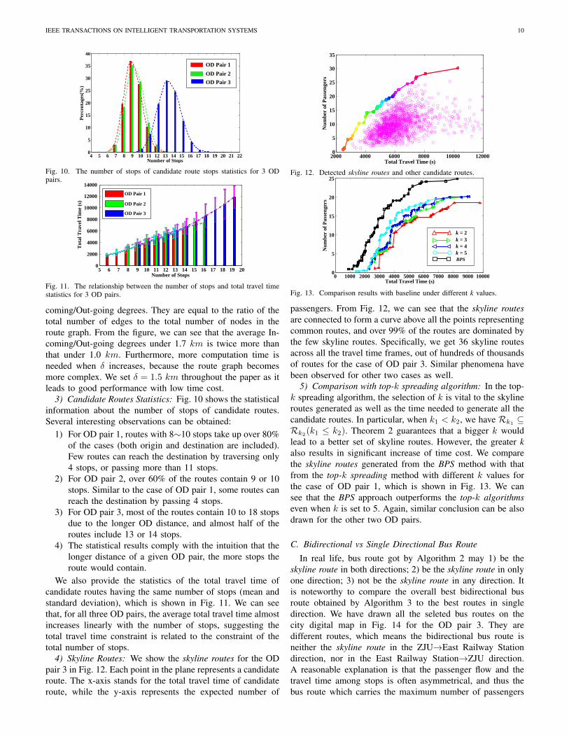
4) Skyline Routes: We show the skyline routes for the ODpair 3 in Fig. 12. Each point in the plane represents a candidateroute. The x-axis stands for the total travel time of candidateroute, while the y-axis represents the expected number of

2000 4000 6000 8000 10000 120000

5

10

15

20

25

30

35

Total Travel Time (s)

Num

ber

of P

asse

nger

s

Fig. 12. Detected skyline routes and other candidate routes.

k = 2k = 3k = 4k = 5BPS

0 1000 2000 3000 4000 5000 6000 7000 8000 9000 100000

5

10

15

20

25

Total Travel Time (s)

Num

ber

of P

asse

nger

s

Fig. 13. Comparison results with baseline under different k values.

passengers. From Fig. 12, we can see that the skyline routesare connected to form a curve above all the points representingcommon routes, and over 99% of the routes are dominated bythe few skyline routes. Specifically, we get 36 skyline routesacross all the travel time frames, out of hundreds of thousandsof routes for the case of OD pair 3. Similar phenomena havebeen observed for other two cases as well.

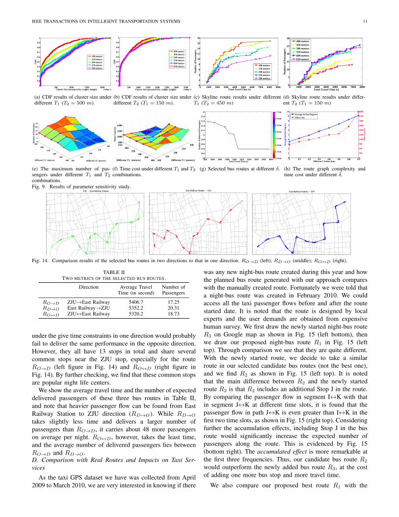
5) Comparison with top-k spreading algorithm: In the top-k spreading algorithm, the selection of k is vital to the skylineroutes generated as well as the time needed to generate all thecandidate routes. In particular, when k1 < k2, we have Rk1 ⊆Rk2(k1 ≤ k2). Theorem 2 guarantees that a bigger k wouldlead to a better set of skyline routes. However, the greater kalso results in significant increase of time cost. We comparethe skyline routes generated from the BPS method with thatfrom the top-k spreading method with different k values forthe case of OD pair 1, which is shown in Fig. 13. We cansee that the BPS approach outperforms the top-k algorithmseven when k is set to 5. Again, similar conclusion can be alsodrawn for the other two OD pairs.

C. Bidirectional vs Single Directional Bus Route

In real life, bus route got by Algorithm 2 may 1) be theskyline route in both directions; 2) be the skyline route in onlyone direction; 3) not be the skyline route in any direction. Itis noteworthy to compare the overall best bidirectional busroute obtained by Algorithm 3 to the best routes in singledirection. We have drawn all the seleted bus routes on thecity digital map in Fig. 14 for the OD pair 3. They aredifferent routes, which means the bidirectional bus route isneither the skyline route in the ZJU→East Railway Stationdirection, nor in the East Railway Station→ZJU direction.A reasonable explanation is that the passenger flow and thetravel time among stops is often asymmetrical, and thus thebus route which carries the maximum number of passengers

IEEE TRANSACTIONS ON INTELLIGENT TRANSPORTATION SYSTEMS 11

500 1000 1500 20000

0.1

0.2

0.3

0.4

0.5

0.6

0.7

0.8

0.9

1

Cluster Size (measured by weight× height)

CD

F

100 meters150 meters200 meters250 meters300 meters

x100m^2

(a) CDF results of cluster size underdifferent T1 (T2 = 500 m).

x100m^2500 1000 1500 2000 2500 3000 35000

0.1

0.2

0.3

0.4

0.5

0.6

0.7

0.8

0.9

1

Cluster Size (measured by weight× height)

CD

F

400 meters450 meters500 meters550 meters600 meters650 meters

(b) CDF results of cluster size underdifferent T2 (T1 = 150 m).

0 1000 2000 3000 4000 5000 6000 7000 8000 90000

2

4

6

8

10

12

14

16

18

Total Travel Time (s)

Num

ber

of P

asse

nger

s

100 meters150 meters200 meters250 meters300 meters

(c) Skyline route results under differentT1 (T2 = 450 m)

0 1000 2000 3000 4000 5000 6000 7000 80000

5

10

15

20

25

30

Total Travel Time (s)

Num

ber

of P

asse

nger

s

400 meters450 meters500 meters550 meters600 meters650 meters

(d) Skyline route results under differ-ent T2 (T1 = 150 m)

100

150

200

250

300

400450

500550

600650

0

5

10

15

20

25

Different T1s(meters)Different T2s (meters)

Num

ber

of P

asse

nger

s

(e) The maximum number of pas-sengers under different T1 and T2combinations.

100150

200250

300

400450

500550

600650800

1000

1200

1400

Different T1s(meters)Different T2s (meters)

Tim

e C

ost (

s)

(f) Time cost under different T1 and T2combinations.

3820 3840 3860 3880 3900 3920 3940 3960 3980 400010

10.2

10.4

10.6

10.8

11

11.2

11.4

11.6

11.8

12

Total Travel Time (s)

Num

ber

of D

eliv

ered

Pas

seng

ers

1.0 km

1.1 km

1.2 km

1.3 km

1.4 km

1.5 km

1.6 km

1.7 km

(g) Selected bus routes at different δ.

1 1.1 1.2 1.3 1.4 1.5 1.6 1.70

1

2

3

4

5

6

7

8

9

10

Ave

rage

In/O

ut D

egre

es

Different δ Values (km)

1 1.1 1.2 1.3 1.4 1.5 1.6 1.70

300

600

900

1200

1500

1800

2100

2400

2700

3000

Tim

e C

ost (

s)

Average In/Out DegreesTime Cost

(h) The route graph complexity andtime cost under different δ.

Fig. 9. Results of parameter sensitivity study.

120.12 120.13 120.14 120.15 120.16 120.17 120.18 120.19 120.2 120.21

30.26

30.265

30.27

30.275

30.28

30.285

30.29

30.295

ZJU → East Railway Station

120.12 120.13 120.14 120.15 120.16 120.17 120.18 120.19 120.2 120.21

30.26

30.265

30.27

30.275

30.28

30.285

30.29

30.295

East Railway Station → ZJU

120.12 120.13 120.14 120.15 120.16 120.17 120.18 120.19 120.2 120.21

30.26

30.265

30.27

30.275

30.28

30.285

30.29

30.295

East Railway Station ↔ ZJU

Fig. 14. Comparison results of the selected bus routes in two directions to that in one direction. RO→D (left); RD→O (middle); RO↔D (right).

TABLE IITWO METRICS OF THE SELECTED BUS ROUTES.

Direction Average Travel Number ofTime (in second) Passengers

RO→D ZJU→East Railway 5406.7 17.25RD→O East Railway→ZJU 5352.2 20.31RO↔D ZJU↔East Railway 5320.2 18.73

under the give time constraints in one direction would probablyfail to deliver the same performance in the opposite direction.However, they all have 13 stops in total and share severalcommon stops near the ZJU stop, especially for the routeRO→D (left figure in Fig. 14) and RO↔D (right figure inFig. 14). By further checking, we find that these common stopsare popular night life centers.

We show the average travel time and the number of expecteddelivered passengers of these three bus routes in Table II,and note that heavier passenger flow can be found from EastRailway Station to ZJU direction (RD→O). While RD→Otakes slightly less time and delivers a larger number ofpassengers than RO→D, it carries about 48 more passengerson average per night. RO↔D, however, takes the least time,and the average number of delivered passengers lies betweenRO→D and RD→O.D. Comparison with Real Routes and Impacts on Taxi Ser-vices

As the taxi GPS dataset we have was collected from April2009 to March 2010, we are very interested in knowing if there

was any new night-bus route created during this year and howthe planned bus route generated with our approach compareswith the manually created route. Fortunately we were told thata night-bus route was created in February 2010. We couldaccess all the taxi passenger flows before and after the routestarted date. It is noted that the route is designed by localexperts and the user demands are obtained from expensivehuman survey. We first draw the newly started night-bus routeR3 on Google map as shown in Fig. 15 (left bottom), thenwe draw our proposed night-bus route R1 in Fig. 15 (lefttop). Through comparison we see that they are quite different.With the newly started route, we decide to take a similarroute in our selected candidate bus routes (not the best one),and we find R2 as shown in Fig. 15 (left top). It is notedthat the main difference between R2 and the newly startedroute R3 is that R2 includes an additional Stop J in the route.By comparing the passenger flow in segment I↔K with thatin segment J↔K at different time slots, it is found that thepassenger flow in path J↔K is even greater than I↔K in thefirst two time slots, as shown in Fig. 15 (right top). Consideringfurther the accumulation effects, including Stop J in the busroute would significantly increase the expected number ofpassengers along the route. This is evidenced by Fig. 15(bottom right). The accumulated effect is more remarkable atthe first three frequencies. Thus, our candidate bus route R2

would outperform the newly added bus route R3, at the costof adding one more bus stop and more travel time.

We also compare our proposed best route R1 with the

IEEE TRANSACTIONS ON INTELLIGENT TRANSPORTATION SYSTEMS 12

TABLE IIITOTAL TRAVEL TIME OF THE BUS ROUTES.

Bus Route Total Travel Time (in second)

R1 3583.8R2 4664.9R3 3624.0

A

B

C

D

F

E

GH

I

J

K

R1

R2

2 4 6 8 10 12 14 160

1

2

3

4

5

6

7

8

9

Bus Frequency

Pas

seng

er F

low

J↔ KI↔ K

R3

2 4 6 8 10 12 14 160

5

10

15

20

25

30

Bus Frequency

Num

ber

of P

asse

nger

s

R

1

R2

R3

R3(March)

Fig. 15. Results comparison. Planned routes (top left); Passenger flowcomparison of two segments at different frequency (top right); Opened night-bus route (bottom left); Number of delivered passengers at different frequency(R1, R2 and R3, bottom right).

candidate route R2. The difference between R1 and R2

lies in two different paths taken from C to H. While R2

passes the famous shopping street (Yan’an Road) in Hangzhou(C ↔ E ↔ F ↔ H), R1 traverses the famous night-clubareas along the West Lake. If we compare the number ofpassengers in R1 and R2, it can be seen from Fig. 15 (rightbottom) that the passenger flow of R2 is heavier than that ofR1 only around 22:00, and it is much lighter soon after 23:00.With the rest of the stops being the same for both R1 andR2, there is no doubt about why R1 has been selected as thebest night-bus route. If we take a closer look at R1, R2, andthe newly started route R3, as R1 takes a much shorter routethan R2 and needs similar travel time as the newly startedroute R3 does (shown in Table III), but R1 expects muchmore passengers than R2 and the newly started route R3, thusit is reasonable to conclude that the selected night-bus routewith our proposed approach is better than the current route-in-service in terms of travel time as well as expected numberof passengers.

It is understood that introducing of new public services (i.e.new Metro/bus lines) would affect taxi services in the city [2].It is interesting to compare the taxi passenger flow changealong the new bus route before/after it was opened. We choosethe new night bus route (R3) opened in February, 2010 forthis study. We prepare taxi GPS data collected in January andMarch, 2010, and calculate the corresponding taxi passengerflow along the new bus route across all bus frequencies, whichis shown in the right bottom subfigure of Fig. 15. We can seethat the number of passengers who travel by taxi along thebus route in March is much smaller but quite stable acrossall the bus frequencies. This may be interpreted by the factthat while some passengers might switch to public services, acertain number of passengers still prefer to take taxis at night.

A B C D G H I J K0

5

10

15

20

Bus Route (Stop Sequence)

Num

ber

of P

asse

nger

s

K J I H G D C B A0

5

10

15

20

Bus Route (Stop Sequence)

Num

ber

of P

asse

nger

s

Fig. 16. The number of passengers on the bus before reaching the stop forOD pair 1.

E. Bus Capacity Analysis

After selecting the best bus route for operation, the nextimportant thing is to determine the proper bus capacity tosave operation cost. The essence for bus capacity estimationis to determine the maximum number of passengers on thebus across all the frequencies. For the bus route R1 of ODpair 1, Fig. 16 shows the number of passengers on the busacross all the frequencies for both directions. As can be seenfrom the results, choosing buses with 20 seats could well meetthe requirements. Besides, we also have the following threeobservations:

1) More passengers are often expected in both directionsfor the first operation frequency, except for the 11th and12th frequencies when the bus runs from C to D.

2) Buses running close to the capacity only last for 3 stops(from A to K) or 4 stops (from K to A).

3) Night buses heading towards different directions havequite different passenger flow patterns.

VI. CONCLUSION AND FUTURE WORK

In this paper, we have investigated the problem of bi-directional night-bus route design by leveraging the taxi GPStraces. The work is motivated by the needs of applyingpervasive sensing, communication and computing technologyfor sustainable city development. To solve the problem, wepropose a two-phase approach for night-bus route planning.In the first phase, we develop a process to cluster “hot”areas with dense passenger pick-up/drop-off, and then proposeeffective methods to split big “hot” areas into clusters andidentify a location in cluster as the candidate bus stop. Inthe second phase, given the bus route origin, destination,candidate bus stops as well as bus operation frequency andmaximum total travel time, we derive several criteria to buildbus route graph and prune the invalid stops and edges itera-tively. Based on the graph, we further develop two heuristicalgorithms to automatically generate candidate bus routes inboth directions, and finally we select the best route whichexpects the maximum number of passengers under the givenconditions. On a real-world dataset which contains morethan 1.57 million passenger delivery trips, we compare ourproposed candidate bus stop identification method with the

IEEE TRANSACTIONS ON INTELLIGENT TRANSPORTATION SYSTEMS 13

popular k-means clustering method and show that our methodcan generate more reasonable and meaningful results. Wefurther extensively evaluate our proposed BPS algorithm forautomatic bus route generation and validate its effectivenessas well as its superior performance over the heuristic top-kspreading algorithm. Further more, we show the selected night-bus route with our proposed approach is better than a newlystarted night-bus route-in-service in Hangzhou, China.

For this work, we consider the effective design of only onebus route. In the future, we plan to broaden and deepen thiswork in several directions. First, we attempt to investigatethe optimal bus route design with more real-life assumptions.For example, for the bus stop identification, the grid cells ingeographical proximity might not be walkable due to physicalbarriers; for bi-directional bus route selection, one-way routesshould be excluded or changed in actual design; Second, wealso plan to explore the issue of designing more than one night-bus route in an optimal way; Third, we would like to developpractical systems leveraging on taxi GPS traces, enabling aseries of pervasive smart transportation services.

ACKNOWLEDGMENTS

The authors want to thank the anonymous reviewers andthe editors for their helpful comments and suggestions. Theauthors would like to thank Shijian Li and Zonghui Wangfor providing the taxi GPS data set, and also thank Lin Sun,Pablo Castro, Tulin Atmaca, Zhu Wang and Zhangbing Zhoufor their valuable inputs. Chao Chen was supported by ChinaScholarship Council (CSC) for his PhD study. This researchwas partly supported by the Institut Mines-TElECOM throughthe “Futur et ruptures” Program, and the National ScienceFoundation of China (61333014, 61105043).

REFERENCES

[1] Public transportation factbook. Technical report, American PublicTransportation Association, 2011.

[2] Zhejiang online news. http://biz.zjol.com.cn/05biz/system/2013/01/25/019113078.shtml, 2013.

[3] C.-N. Anagnostopoulos, I. Anagnostopoulos, V. Loumos, andE. Kayafas. A license plate-recognition algorithm for intelligenttransportation system applications. IEEE Transactions on IntelligentTransportation Systems, 7(3):377–392, 2006.

[4] D. L. Applegate, R. E. Bixby, V. Chvatal, and W. J. Cook. The TravelingSalesman Problem: A Computational Study. Princeton University Press,2007.

[5] J. Aslam, S. Lim, and X. Pan. City-scale traffic estimation from a rovingsensor network. In Proc. of ACM SenSys, 2012.

[6] R. K. Balan, K. X. Nguyen, and L. Jiang. Real-time trip informationservice for a large taxi fleet. In Proc. of MobiSys, pages 99–112, 2011.

[7] F. Bastani, Y. Huang, X. Xie, and J. W. Powell. A greener transportationmode: flexible routes discovery from GPS trajectory data. In Proc. ofGIS, pages 405–408, 2011.

[8] S. Borzsony, D. Kossmann, and K. Stocker. The skyline operator. InProc. of ICDE, pages 421–430, 2001.

[9] P. S. Castro, D. Zhang, C. Chen, S. Li, and G. Pan. From taxi GPStraces to social and community dynamics: A survey. ACM ComputingSurveys, 46(2):17:1–17:34, 2013.

[10] P. S. Castro, D. Zhang, and S. Li. Urban traffic modelling and predictionusing large scale taxi GPS traces. In Proc. Pervasive Computing, pages57–72, 2012.

[11] A. Ceder and N. Wilson. Bus network design. Transportation ResearchPart B: Methodological, 20(4):331–344, 1986.

[12] S. Chawla, Y. Zheng, and J. Hu. Inferring the root cause in road trafficanomalies. In Proc. of ICDM, pages 141–150, 2012.

[13] C. Chen, D. Zhang, P. Castro, N. Li, L. Sun, S. Li, and Z. Wang. iBOAT:Isolation-based online anomalous trajectory detection. IEEE Transac-tions on Intelligent Transportation Systems, 14(2):806–818, 2013.

[14] C. Chen, D. Zhang, Z.-H. Zhou, N. Li, T. Atmaca, and S. Li. B-Planner:Night bus route planning using large-scale taxi GPS traces. In Proc. ofPerCom, pages 225–233, 2013.

[15] T. A. Chua. The planning of urban bus routes and frequencies: A survey.Transportation, 12(2):147–172, 1984.

[16] d’Orey and P. M. Empirical evaluation of a dynamic and distributed taxi-sharing system. In Proc. of IEEE Conference on ITS, pages 140–146,2012.

[17] Y. Ge, H. Xiong, C. Liu, and Z.-H. Zhou. A taxi driving fraud detectionsystem. In Proc. of ICDM, pages 181–190, 2011.

[18] Y. Ge, H. Xiong, A. Tuzhilin, K. Xiao, M. Gruteser, and M. Pazzani.An energy-efficient mobile recommender system. In Proc. of ACMSIGKDD, pages 899–908, 2010.

[19] V. Guihaire and J.-K. Hao. Transit network design and scheduling: Aglobal review. Transportation Research Part A: Policy and Practice,42(10):1251 – 1273, 2008.

[20] A. Hofleitner, R. Herring, P. Abbeel, and A. Bayen. Learning thedynamics of arterial traffic from probe data using a dynamic Bayesiannetwork. IEEE Transactions on Intelligent Transportation Systems,(99):1–15, 2012.

[21] H. Hu, Z. Wu, B. Mao, Y. Zhuang, J. Cao, and J. Pan. Pick-up tree basedroute recommendation from taxi trajectories. In Web-Age InformationManagement, volume 7418, pages 471–483. 2012.

[22] S. Jerby and A. Ceder. Optimal routing design for shuttle bus service.Transportation Research Record: Journal of the Transportation ResearchBoard, 1971:14–22, 2006.

[23] S. Kim, S. Shekhar, and M. Min. Contraflow transportation networkreconfiguration for evacuation route planning. IEEE Transactions onKnowledge and Data Engineering, 20(8):1115–1129, 2008.

[24] B. Li, D. Zhang, L. Sun, C. Chen, S. Li, G. Qi, and Q. Yang. Huntingor waiting? Discovering passenger-finding strategies from a large-scalereal-world taxi dataset. In Proc. of PerCom Workshop, pages 63 –68,2011.

[25] Q. Li, Z. Zeng, T. Zhang, J. Li, and Z. Wu. Path-finding throughflexible hierarchical road networks: An experiential approach using taxitrajectory data. International Journal of Applied Earth Observation andGeoinformation, 13(1):110 – 119, 2011.

[26] C.-L. Liu, T.-W. Pai, C.-T. Chang, and C.-M. Hsieh. Path-planning al-gorithms for public transportation systems. In Proc. of IEEE Conferenceon ITS, pages 1061–1066, 2001.

[27] L. Liu, C. Andris, and C. Ratti. Uncovering cabdrivers’ behavior patternsfrom their digital traces. Computers, Environment and Urban Systems,34(6):541 – 548, 2010.

[28] W. Liu, Y. Zheng, S. Chawla, J. Yuan, and X. Xing. Discovering spatio-temporal causal interactions in traffic data streams. In Proc. of ACMSIGKDD, pages 1010–1018, 2011.

[29] Y. Liu, F. Wang, Y. Xiao, and S. Gao. Urban land uses and traffic‘source-sink areas’: Evidence from GPS-enabled taxi data in Shanghai.Landscape and Urban Planning, 106(1):73 – 87, 2012.

[30] S. Ma, Y. Zheng, and O. Wolfson. T-share: A large-scale dynamic taxirideesharing service. In Proc. of ICDE, 2013.

[31] B. M.H. and M. H.S. TRUST: A lisp program for the analysis of transitroute configurations. Transportation Research Record, 1283:125–135,1990.

[32] G. F. Newell. Some issues relating to the optimal design of bus routes.Transportation Science, 13(1):20–35, 1979.

[33] G. Pan, G. Qi, Z. Wu, D. Zhang, and S. Li. Land-use classificationusing taxi GPS traces. IEEE Transactions on Intelligent TransportationSystems, 14(1):113–123, 2013.

[34] S. Pattnaik, S. Mohan, and V. Tom. Urban bus transit route networkdesign using genetic algorithm. Journal of Transportation Engineering,124(4):368–375, 1998.

[35] J. Powell, Y. Huang, F. Bastani, and M. Ji. Towards reducing taxicabcruising time using spatio-temporal profitability maps. In Advances inSpatial and Temporal Databases, volume 6849, pages 242–260. 2011.

[36] L. Sun, D. Zhang, C. Chen, P. S. Castro, S. Li, and Z. Wang. Realtime anomalous trajectory detection and analysis. Mobile Networks andApplications, 18(3):341–356, 2013.

[37] W. Szeto and Y. Wu. A simultaneous bus route design and frequencysetting problem for Tin Shui Wai, Hong Kong. European Journal ofOperational Research, 209(2):141 – 155, 2011.

[38] F.-Y. Wang. Driving into the future with ITS. IEEE Intelligent Systems,21(3):94–95, 2006.

IEEE TRANSACTIONS ON INTELLIGENT TRANSPORTATION SYSTEMS 14

[39] F.-Y. Wang. Parallel control and management for intelligent transporta-tion systems: Concepts, architectures, and applications. IEEE Transac-tions on Intelligent Transportation Systems, 11(3):630–638, 2010.

[40] Z. Wang and J. Crowcroft. Analysis of shortest-path routing algorithmsin a dynamic network environment. SIGCOMM Comput. Commun. Rev.,22(2):63–71, 1992.

[41] H. wen Chang, Y. chin Tai, and J. Y. jen Hsu. Context-aware taxi demandhotspots prediction. International Journal of Business Intelligence andData Mining, 5(1):3–18, 2010.

[42] J. Yuan, Y. Zheng, and X. Xie. Discovering regions of different functionsin a city using human mobility and POIs. In Proc. of ACM SIGKDD,pages 186–194, 2012.

[43] J. Yuan, Y. Zheng, X. Xie, and G. Sun. T-drive: Enhancing driving direc-tions with taxi drivers’ intelligence. IEEE Transactions on Knowledgeand Data Engineering, 25(1):220–232, 2013.

[44] N. J. Yuan, Y. Zheng, L. Zhang, and X. Xie. T-finder: A recommendersystem for finding passengers and vacant taxis. IEEE Transactions onKnowledge and Data Engineering, page to appear, 2013.

[45] D. Zhang, B. Guo, and Z. Yu. The emergence of social and communityintelligence. IEEE Computer, 44(7):21–28, 2011.

[46] D. Zhang, N. Li, Z.-H. Zhou, C. Chen, L. Sun, and S. Li. iBAT:Detecting anomalous taxi trajectories from GPS traces. In Proc. ofUbiComp, pages 99–108, 2011.

[47] J. Zhang, F.-Y. Wang, K. Wang, W.-H. Lin, X. Xu, and C. Chen. Data-driven intelligent transportation systems: A survey. IEEE Transactionson Intelligent Transportation Systems, 12(4):1624–1639, 2011.

[48] Z. Zhang, D. Yang, T. Zhang, Q. He, and X. Lian. A study on the methodfor cleaning and repairing the probe vehicle data. IEEE Transactionson Intelligent Transportation Systems, 14(1):419–427, 2013.

[49] F. Zhao and X. Zeng. Optimization of transit route network, vehicleheadways and timetables for large-scale transit networks. EuropeanJournal of Operational Research, 186(2):841 – 855, 2008.

[50] Y. Zheng, Y. Liu, J. Yuan, and X. Xie. Urban computing with taxicabs.In Proc. of UbiComp, pages 89–98, 2011.

Chao Chen received the B.Sc. and M.Sc. degrees incontrol science and control engineering from North-western Polytechnical University, Xi’an, China, in2007 and 2010, respectively. He is currently workingtoward the Ph.D. degree with Pierre and Marie CurieUniversity, Paris, France, and with Institut Mines-TELECOM/TELECOM SudParis, Evry, France. Mr.Chen was a co-recipient of the Best Paper Runner-Up Award at MobiQuitous 2011.

In 2009, he worked as a Research Assistant withHong Kong Polytechnic University, Kowloon, Hong

Kong. His research interests include pervasive computing, social networkanalysis, and data mining from large-scale taxi data.

Daqing Zhang is a professor at Institut Mines-TELECOM/TELECOM SudParis, France. He ob-tained his Ph.D from University of Rome “La S-apienza” and the University of L’Aquila, Italy in1996. His research interests include large-scale datamining, urban computing, context-aware computing,and ambient assistive living. He has published morethan 180 referred journal and conference papers,all his research has been motivated by practicalapplications in digital cities, mobile social networksand elderly care.

Dr. Zhang is the Associate Editor for four journals including ACM Trans-actions on Intelligent Systems and Technology. He has been a frequent InvitedSpeaker in various international events on ubiquitous computing. He is thewinner of the Ten Years CoMoRea Impact Paper Award at IEEE PerCom2013, the Best Paper Award at IEEE UIC 2012 and the Best Paper RunnerUp Award at Mobiquitous 2011.

Nan Li received the MSc degree in computer sci-ence from Nanjing University, China, in 2008. Atthe same year, he became a faculty member inthe School of Mathematical Sciences at SoochowUniversity, China. He is currently pursuing the PhDdegree in the Department of Computer Science &Technology of Nanjing University. His research in-terests are mainly in machine learning, data miningand ambient intelligence. He and other LAMDAmembers won the Grand Prize (Open Category) inthe PAKDD 2012 Data Mining Competition. His co-

authored paper won the Best Paper Runner-Up Award at MobiQuitous 2011.He has been awarded with the IBM PhD Fellowship (2013-2014) and theBaidu Fellowship (2013-2014).

Zhi-Hua Zhou (S00-M01-SM06-F13) received theBSc, MSc and PhD degrees in computer sciencefrom Nanjing University, China, in 1996, 1998 and2000, respectively, all with the highest honors. Hejoined the Department of Computer Science & Tech-nology at Nanjing University as an assistant profes-sor in 2001, and is currently professor and Directorof the LAMDA group. His research interests aremainly in artificial intelligence, machine learning,data mining, pattern recognition and multimediainformation retrieval. In these areas he has published

over 90 papers in leading international journals or conference proceedings,and holds 12 patents. He has won various awards/honors including theNational Science & Technology Award for Young Scholars of China, theFok Ying Tung Young Professorship 1st-Grade Award, the Microsoft YoungProfessorship Award and eight international journals/conferences paper awardsand competition awards.

He is an Executive Editor-in-Chief of the Frontiers of Computer Science,Associate Editor-in-Chief of the Chinese Science Bulletin, Associate Editor oreditorial boards member of the ACM Transactions on Intelligent Systems andTechnology, IEEE Transactions on Neural Networks and Learning Systems,and many other journals. He served as Associate Editor for IEEE Transac-tions on Knowledge and Data Engineering (2008-2012) and Knowledge andInformation Systems (2003-2008). He is the founder and Steering CommitteeChair of ACML, and Steering Committee member of PAKDD and PRICAI.He serves/ed as General Chair/Co-chair of ACML12, ADMA12, PCM13,PAKDD14, Program Chair/Co-Chair of PAKDD07, PRICAI08, ACML09,SDM13, etc., Workshop Chair/Co-Chair of KDD12 and ICDM14, TutorialChair/Co-Chair of KDD13 and CIKM14, and Program Vice Chair or AreaChair of various conferences such as ICML, IJCAI, AAAI, ICPR, etc. Heis the Chair of the Machine Learning Technical Committee of the ChineseAssociation of Artificial Intelligence, Chair of the Artificial Intelligence &Pattern Recognition Technical Committee of the China Computer Federation,Vice Chair of the Data Mining Technical Committee of IEEE ComputationalIntelligence Society and the Chair of the IEEE Computer Society NanjingChapter. He is an IEEE Fellow, IAPR Fellow, IET/IEE Fellow and ACMDistinguished Scientist.