IEEE TRANSACTIONS ON INFORMATION THEORY, VOL. 55, NO. 9, SEPTEMBER

IEEE TRANSACTIONS ON INFORMATION THEORY, VOL. 55, NO. 9, SEPTEMBER 2009 4067

Interference and Outage in Clustered WirelessAd Hoc Networks

Radha Krishna Ganti, Student Member, IEEE, and Martin Haenggi, Senior Member, IEEE

Abstract—In the analysis of large random wireless networks,the underlying node distribution is almost ubiquitously assumedto be the homogeneous Poisson point process. In this paper, thenode locations are assumed to form a Poisson cluster process onthe plane. We derive the distributional properties of the inter-ference and provide upper and lower bounds for its distribution.We consider the probability of successful transmission in aninterference-limited channel when fading is modeled as Rayleigh.We provide a numerically integrable expression for the outageprobability and closed-form upper and lower bounds. We showthat when the transmitter–receiver distance is large, the successprobability is greater than that of a Poisson arrangement. Theseresults characterize the performance of the system under geo-graphical or MAC-induced clustering. We obtain the maximumintensity of transmitting nodes for a given outage constraint, i.e.,the transmission capacity (of this spatial arrangement) and showthat it is equal to that of a Poisson arrangement of nodes. Forthe analysis, techniques from stochastic geometry are used, inparticular the probability generating functional of Poisson clusterprocesses, the Palm characterization of Poisson cluster processes,and the Campbell–Mecke theorem.

Index Terms—Interference, Poisson cluster processes, shot noise,transmission capacity, wireless networks.

I. INTRODUCTION

A COMMON and analytically convenient assumption forthe node distribution in large wireless networks is the ho-

mogeneous (or stationary) Poisson point process (PPP) of in-tensity , where the number of nodes in a certain area of size

is Poisson with parameter , and the numbers of nodes intwo disjoint areas are independent random variables. For sensornetworks, this assumption is usually justified by claiming thatsensor nodes may be dropped from aircraft in large numbers; formobile ad hoc networks, it may be argued that terminals moveindependently from each other. While this may be the case forcertain networks, it is much more likely that the node distribu-tion is not ”completely spatially random,” i.e., that nodes areeither clustered or more regularly distributed. Moreover, evenif the complete set of nodes constitutes a PPP, the subset of ac-tive nodes (e.g., transmitters in a given time slot or sentries in

Manuscript received June 16, 2007; revised September 19, 2008. Current ver-sion published August 19, 2009. This work was supported by the NSF underGrants CNS 04-47869, CCF 05-15012, and DMS 505624, and the DARPA/IT-MANET program under Grant W911NF-07-1-0028. The material in this paperwas presented in part at the 40th Asilomar Conference on Signal, Systems, andComputers, Pacific Grove, CA, October 2006.

The authors are with the Department of Electrical Engineering, Univer-sity of Notre Dame, Notre Dame, IN 46556 USA (e-mail: [email protected];[email protected]).

Communicated by A. J. Grant, Associate Editor for Communications.Color versions of Figures 1 and 3–9 in this paper are available online at http://

ieeexplore.ieee.org.Digital Object Identifier 10.1109/TIT.2009.2025543

a sensor network) may not be homogeneously Poisson. On theone hand, it seems preferable that simultaneous transmitters inan ad hoc network or sentries in a sensor network form moreregular processes to maximize spatial reuse or coverage, respec-tively. On the other hand, many protocols have been suggestedthat are based on clustered processes where the clustering is “ar-tificially” induced by mediaum access control (MAC) protocols.This motivates the need to extend the rich set of results availablefor PPPs to other node distributions. The clustering of nodesmay also be due to geographical factors, for example, commu-nicating nodes inside a building or groups of nodes moving in acoordinated fashion. We denote the former as logical clusteringand the latter as geographical clustering. The main motivationof this paper is to understand the characteristics of the interfer-ence when the transmitting nodes are clustered.

A. Related Work

There exists a significant body of literature for networks withPoisson distributed nodes. In [1], the characteristic function ofthe interference was obtained when there was no fading and thenodes were Poisson distributed. They also provide the proba-bility distribution function of the interference as an infinite se-ries. Mathar et al., in [2], analyze the interference when the in-terference contribution by a transmitter located at to a receiverlocated at the origin is exponentially distributed with param-eter . Using this model they derive the density function ofthe interference when the nodes are arranged as a one-dimen-sional lattice. Also the Laplace transform of the interference isobtained when the nodes are Poisson distributed.

It is known that the interference in a planar network of nodescan be modeled as a shot-noise process. Let be a pointprocess in . Let be a sequence of independent andidentically distributed (i.i.d.) random functions on , indepen-dent of . Then a generalized shot-noise process can be de-fined as [3]

If is the path loss model with fading, is the interfer-ence at location if all nodes are transmitting. The shot-noiseprocess is a very well studied process for noise modeling. It wasfirst introduced by Schottky in the study of fluctuations in theanode current of a thermionic diode, and it was studied in de-tail by Rice [4], [5]. Daley in 1971 defined multidimensionalshot noise and examined its existence when the pointsare Poisson distributed in . The existence of a generalizedshot-noise process, defined for any point process, was studied byWestcott in [3]. Westcott also provides the Laplace transform of

0018-9448/$26.00 © 2009 IEEE

Authorized licensed use limited to: UNIVERSITY NOTRE DAME. Downloaded on August 25, 2009 at 15:14 from IEEE Xplore. Restrictions apply.

4068 IEEE TRANSACTIONS ON INFORMATION THEORY, VOL. 55, NO. 9, SEPTEMBER 2009

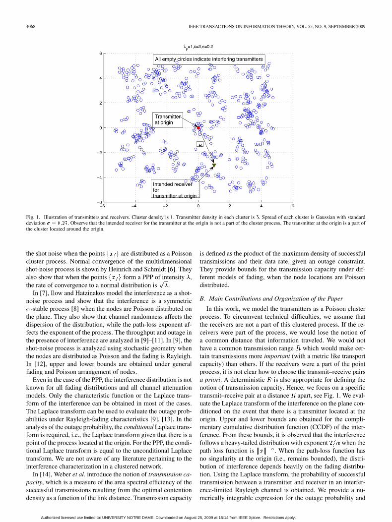
Fig. 1. Illustration of transmitters and receivers. Cluster density is �. Transmitter density in each cluster is �. Spread of each cluster is Gaussian with standarddeviation � � ��. Observe that the intended receiver for the transmitter at the origin is not a part of the cluster process. The transmitter at the origin is a part ofthe cluster located around the origin.

the shot noise when the points are distributed as a Poissoncluster process. Normal convergence of the multidimensionalshot-noise process is shown by Heinrich and Schmidt [6]. Theyalso show that when the points form a PPP of intensity ,the rate of convergence to a normal distribution is .

In [7], Ilow and Hatzinakos model the interference as a shot-noise process and show that the interference is a symmetric

-stable process [8] when the nodes are Poisson distributed onthe plane. They also show that channel randomness affects thedispersion of the distribution, while the path-loss exponent af-fects the exponent of the process. The throughput and outage inthe presence of interference are analyzed in [9]–[11]. In [9], theshot-noise process is analyzed using stochastic geometry whenthe nodes are distributed as Poisson and the fading is Rayleigh.In [12], upper and lower bounds are obtained under generalfading and Poisson arrangement of nodes.

Even in the case of the PPP, the interference distribution is notknown for all fading distributions and all channel attenuationmodels. Only the characteristic function or the Laplace trans-form of the interference can be obtained in most of the cases.The Laplace transform can be used to evaluate the outage prob-abilities under Rayleigh-fading characteristics [9], [13]. In theanalysis of the outage probability, the conditional Laplace trans-form is required, i.e., the Laplace transform given that there is apoint of the process located at the origin. For the PPP, the condi-tional Laplace transform is equal to the unconditional Laplacetransform. We are not aware of any literature pertaining to theinterference characterization in a clustered network.

In [14], Weber et al. introduce the notion of transmission ca-pacity, which is a measure of the area spectral efficiency of thesuccessful transmissions resulting from the optimal contentiondensity as a function of the link distance. Transmission capacity

is defined as the product of the maximum density of successfultransmissions and their data rate, given an outage constraint.They provide bounds for the transmission capacity under dif-ferent models of fading, when the node locations are Poissondistributed.

B. Main Contributions and Organization of the Paper

In this work, we model the transmitters as a Poisson clusterprocess. To circumvent technical difficulties, we assume thatthe receivers are not a part of this clustered process. If the re-ceivers were part of the process, we would lose the notion ofa common distance that information traveled. We would nothave a common transmission range which would make cer-tain transmissions more important (with a metric like transportcapacity) than others. If the receivers were a part of the pointprocess, it is not clear how to choose the transmit–receive pairsa priori. A deterministic is also appropriate for defining thenotion of transmission capacity. Hence, we focus on a specifictransmit–receive pair at a distance apart, see Fig. 1. We eval-uate the Laplace transform of the interference on the plane con-ditioned on the event that there is a transmitter located at theorigin. Upper and lower bounds are obtained for the compli-mentary cumulative distribution function (CCDF) of the inter-ference. From these bounds, it is observed that the interferencefollows a heavy-tailed distribution with exponent when thepath loss function is . When the path-loss function hasno singularity at the origin (i.e., remains bounded), the distri-bution of interference depends heavily on the fading distribu-tion. Using the Laplace transform, the probability of successfultransmission between a transmitter and receiver in an interfer-ence-limited Rayleigh channel is obtained. We provide a nu-merically integrable expression for the outage probability and


GANTI AND HAENGGI: INTERFERENCE AND OUTAGE IN CLUSTERED WIRELESS Ad Hoc NETWORKS 4069

closed-form upper and lower bounds. The clustering gainis defined as the ratio of success probabilities of the clusteredprocess and the PPP with the same intensity. It is observed thatwhen the transmitter–receiver distance is large, the clusteringgain is greater than unity and becomes infinity as .The gain at small depends on the path loss model andthe total intensity of transmissions. We provide conditions onthe total intensity of transmitters under which the gain is greaterthan unity for small . This is useful to determine when logicalclustering performs better than uniform deployment of nodes.We also obtain the maximum intensity of transmitting nodes fora given outage constraint, i.e., the transmission capacity [12],[14], [15] of this spatial arrangement and show that it is equalto that of a Poisson arrangement of nodes. We observe that in aspread-spectrum system, clustering is beneficial for long-rangetransmissions, and we compare DS-CDMA and FH-CDMA.

The paper is organized as follows: in Section II, wepresent the system model and assumptions, introduce theNeyman–Scott cluster process and derive its conditional gen-erating functional. In Section III, we derive the properties ofinterference, outage probability and the gain function . InSection IV, we derive the transmission capacity of the clusterednetwork.

II. SYSTEM MODEL AND ASSUMPTIONS

In this section, we introduce the system model and derivesome required results for the Poisson cluster process.

A. System Model and Notation

The location of transmitting nodes is modeled as a stationaryand isotropic Poisson cluster process on . More detailsabout this spatial process are given in Section II-B. The receiveris not considered a part of the process; see Fig. 1. Each trans-mitter is assumed to transmit at unit power. The power receivedby a receiver located at due to a transmitter at is modeledas , where is the power fading coefficient (squareof the amplitude fading coefficient) associated with the channelbetween the nodes and . We also assume that the fading co-efficients are i.i.d.. Let denote the origin . We assumethat the path loss model satisfies thefollowing conditions.

1) is a continuous, positive, nonincreasing function ofand

where denotes a ball of radius around the origin.2)

(1)

is usually taken to be a power law in the formor . To satisfy Condition 1, we

require . The interference at node on the plane is givenby

(2)

The conditions required for the existence of are discussedin [3]. Let denote the additive Gaussian noise at the receiver.We say that the communication from a transmitter at the originto a receiver situated at is successful if and only if

(3)

or equivalently

For the calculation of the outage probability and transmissioncapacity, the amplitude fading is assumed to be Rayleighwith , but some results are presented for the moregeneral case of Nakagami- fading. Hence, the powers areexponentially and gamma distributed, respectively. We will beevaluating the performance of spread spectrum in some sec-tions of the paper. Even though we evaluate spread-spectrumsystems (specifically DS-CDMA and FH-CDMA), we will notbe using any power control, the reason being that there is nocentral base station. One can think of using the spread spectrumas a method of multiple access. The main difference betweenDS-CDMA and FH-CDMA in our context is that DS-CDMAeffectively reduces the threshold by the spreading gain, whilein FH-CDMA the number of contending transmitters is reducedby a similar factor.

Notation: If we shall useif if and if

.

B. Neyman–Scott Cluster Processes

Neyman–Scott cluster processes [16] are Poisson cluster pro-cesses that result from homogeneous independent clustering ap-plied to a stationary Poisson process, i.e., the parent points forma stationary Poisson process of intensity .The clusters are of the form for each . Theare a family of i.i.d. finite point sets with distribution indepen-dent of the parent process. The complete process is given by

(4)

The parent points themselves are not included. The daughterpoints of the representative cluster are scattered indepen-dently and with identical distribution

, around the origin. We also assume that the scattering densityof the daughter process is isotropic. This makes the process

isotropic. The intensity of the cluster process is ,where is the average number of points in representative cluster.

We further focus on more specific models for the represen-tative cluster, namely Matern cluster processes and Thomascluster processes. In these processes, the number of points in therepresentative cluster is Poisson distributed with mean . Forthe Matern cluster process, each point is uniformly distributedin a ball of radius around the origin. So the density function

is given by

otherwise.(5)



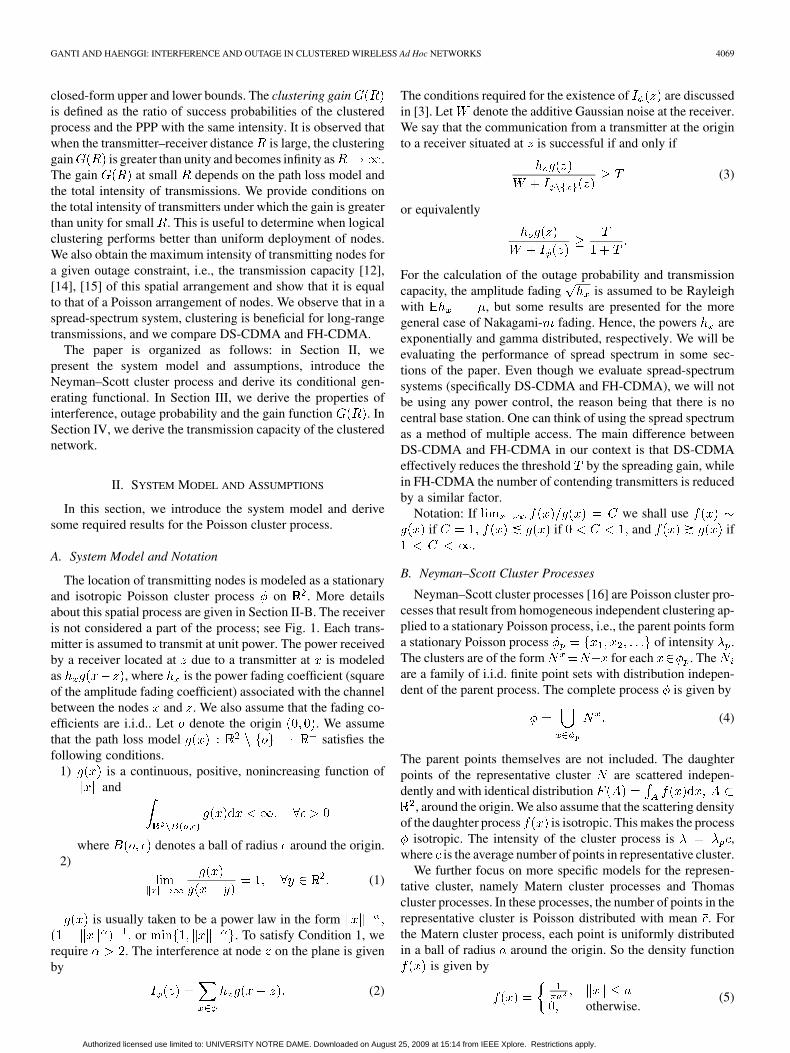
Fig. 2. (Left) Thomas cluster process with parameters � � �� and � � ��. The crosses indicate the parent points. (Right) PPP with the same intensity� � � for comparison.

In the Thomas cluster process, each point is scattered usinga symmetric normal distribution with variance around theorigin. So the density function is given by

A Thomas cluster process is illustrated in Fig. 2. Neyman–Scottcluster processes are also Cox processes [16] if the number ofpoints in the daughter cluster are Poisson distributed. The den-sity of the driving random measure in this case is

Let denote the expectation with respect to the reducedPalm measure [16], [17]. It is basically the conditional expecta-tion for point processes, given that there is a point of the processat the origin but without including the point. Let

and . When is Poisson of inten-sity , the conditional generating functional is

(6)

The generating functional of theNeyman–Scott cluster process is given by [16], [18]

where is the moment generating functionof the number of points in the representative cluster. When the

number of points in the representative cluster is Poisson withmean , as in the case of Matern and Thomas cluster processes,the moment generating function is given by

The generating functional for the representative clusteris given by [18], [19]

The reduced Palm distribution of a Neyman–Scott clusterprocess is given by [16]–[18], [20]

(7)

where is the distribution of , and is the reduced Palmdistribution of the finite representative cluster process . “*”denotes the convolution of distributions, which corresponds tothe superposition of and . The reduced Palm distribution

is given by

(8)

where is a translated point process. We require thefollowing lemma to evaluate the conditional Laplace transformof the interference. Let denote the conditional generatingfunctional of the Neyman–Scott cluster process, i.e.,

(9)

We will use a dot to indicate the variable which the functionalis acting on. For example .



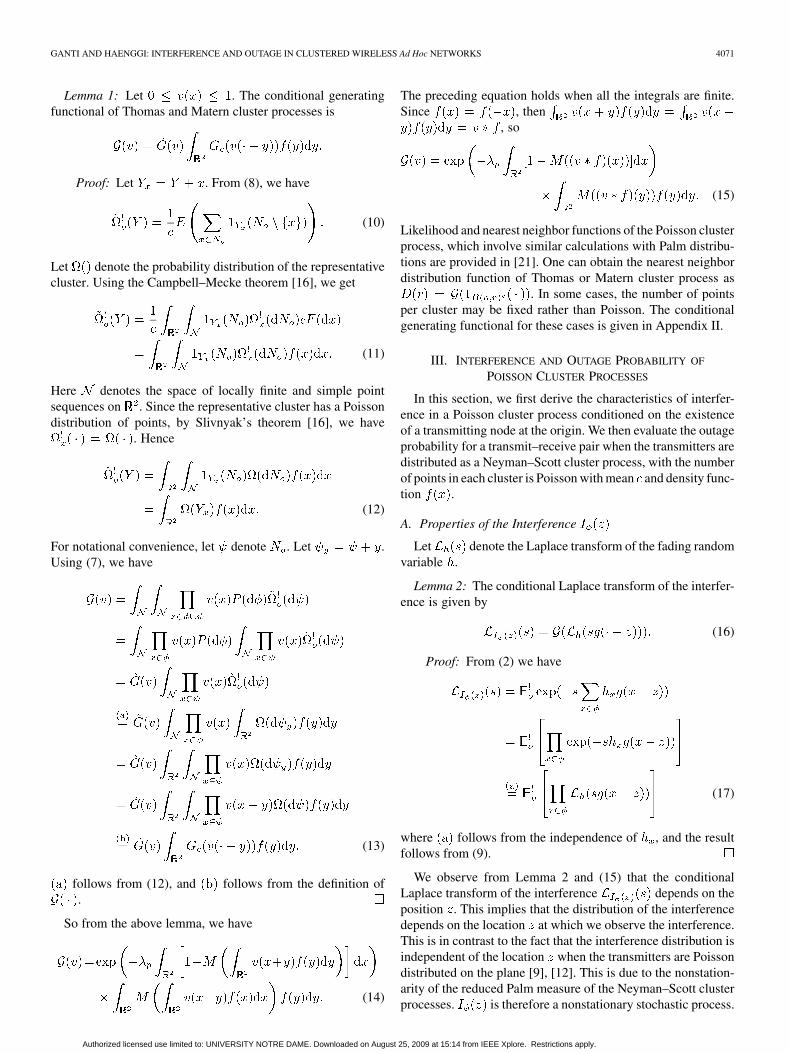
Lemma 1: Let . The conditional generatingfunctional of Thomas and Matern cluster processes is

Proof: Let . From (8), we have

(10)

Let denote the probability distribution of the representativecluster. Using the Campbell–Mecke theorem [16], we get

(11)

Here denotes the space of locally finite and simple pointsequences on . Since the representative cluster has a Poissondistribution of points, by Slivnyak’s theorem [16], we have

. Hence

(12)

For notational convenience, let denote . Let .Using (7), we have

(13)

follows from (12), and follows from the definition of.

So from the above lemma, we have

(14)

The preceding equation holds when all the integrals are finite.Since , then

, so

(15)

Likelihood and nearest neighbor functions of the Poisson clusterprocess, which involve similar calculations with Palm distribu-tions are provided in [21]. One can obtain the nearest neighbordistribution function of Thomas or Matern cluster process as

. In some cases, the number of pointsper cluster may be fixed rather than Poisson. The conditionalgenerating functional for these cases is given in Appendix II.

III. INTERFERENCE AND OUTAGE PROBABILITY OF

POISSON CLUSTER PROCESSES

In this section, we first derive the characteristics of interfer-ence in a Poisson cluster process conditioned on the existenceof a transmitting node at the origin. We then evaluate the outageprobability for a transmit–receive pair when the transmitters aredistributed as a Neyman–Scott cluster process, with the numberof points in each cluster is Poisson with mean and density func-tion .

A. Properties of the Interference

Let denote the Laplace transform of the fading randomvariable .

Lemma 2: The conditional Laplace transform of the interfer-ence is given by

(16)

Proof: From (2) we have

(17)

where follows from the independence of , and the resultfollows from (9).

We observe from Lemma 2 and (15) that the conditionalLaplace transform of the interference depends on theposition . This implies that the distribution of the interferencedepends on the location at which we observe the interference.This is in contrast to the fact that the interference distribution isindependent of the location when the transmitters are Poissondistributed on the plane [9], [12]. This is due to the nonstation-arity of the reduced Palm measure of the Neyman–Scott clusterprocesses. is therefore a nonstationary stochastic process.



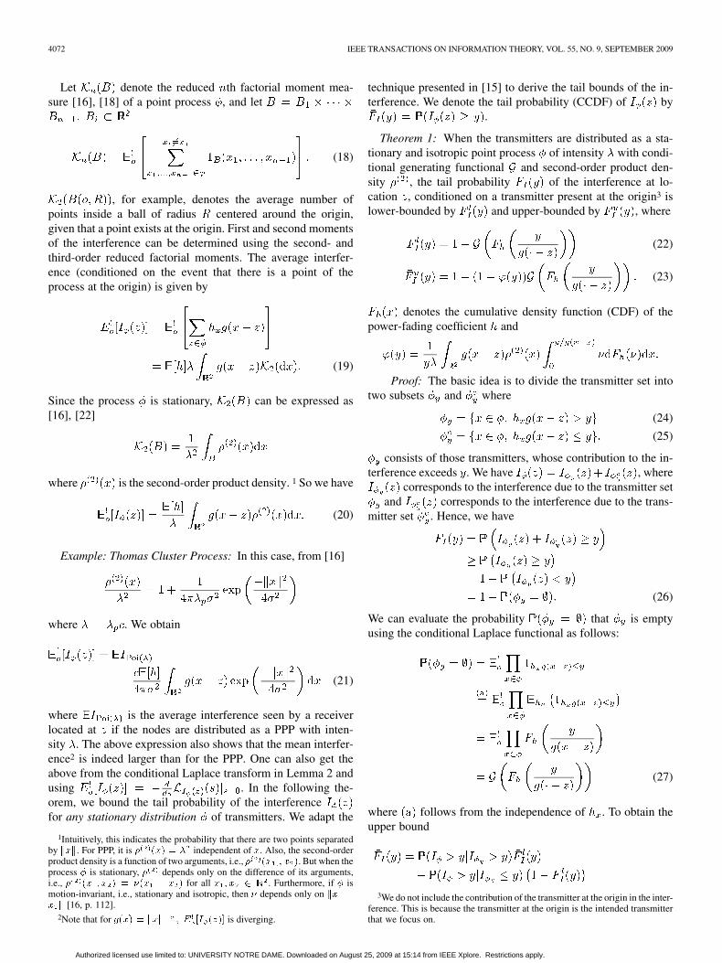
Let denote the reduced th factorial moment mea-sure [16], [18] of a point process , and let

(18)

, for example, denotes the average number ofpoints inside a ball of radius centered around the origin,given that a point exists at the origin. First and second momentsof the interference can be determined using the second- andthird-order reduced factorial moments. The average interfer-ence (conditioned on the event that there is a point of theprocess at the origin) is given by

(19)

Since the process is stationary, can be expressed as[16], [22]

where is the second-order product density. 1 So we have

(20)

Example: Thomas Cluster Process: In this case, from [16]

where . We obtain

(21)

where is the average interference seen by a receiverlocated at if the nodes are distributed as a PPP with inten-sity . The above expression also shows that the mean interfer-ence2 is indeed larger than for the PPP. One can also get theabove from the conditional Laplace transform in Lemma 2 andusing . In the following the-orem, we bound the tail probability of the interferencefor any stationary distribution of transmitters. We adapt the

1Intuitively, this indicates the probability that there are two points separatedby ��. For PPP, it is � �� independent of �. Also, the second-orderproduct density is a function of two arguments, i.e., � �� . But when theprocess � is stationary, � depends only on the difference of its arguments,i.e., � �� for all � � � � . Furthermore, if � ismotion-invariant, i.e., stationary and isotropic, then � depends only on �� [16, p. 112].

2Note that for �� is diverging.

technique presented in [15] to derive the tail bounds of the in-terference. We denote the tail probability (CCDF) of by

.

Theorem 1: When the transmitters are distributed as a sta-tionary and isotropic point process of intensity with condi-tional generating functional and second-order product den-sity , the tail probability of the interference at lo-cation , conditioned on a transmitter present at the origin3 islower-bounded by and upper-bounded by , where

(22)

(23)

denotes the cumulative density function (CDF) of thepower-fading coefficient and

Proof: The basic idea is to divide the transmitter set intotwo subsets and where

(24)

(25)

consists of those transmitters, whose contribution to the in-terference exceeds . We have , where

corresponds to the interference due to the transmitter setand corresponds to the interference due to the trans-

mitter set . Hence, we have

(26)

We can evaluate the probability that is emptyusing the conditional Laplace functional as follows:

(27)

where follows from the independence of . To obtain theupper bound

3We do not include the contribution of the transmitter at the origin in the inter-ference. This is because the transmitter at the origin is the intended transmitterthat we focus on.



where follows from the lower bound we have established.To evaluate we use the Markov inequality.We have

(28)

follows from the Markov inequality, and follows froma procedure similar to the calculation of the mean interferencein (20).

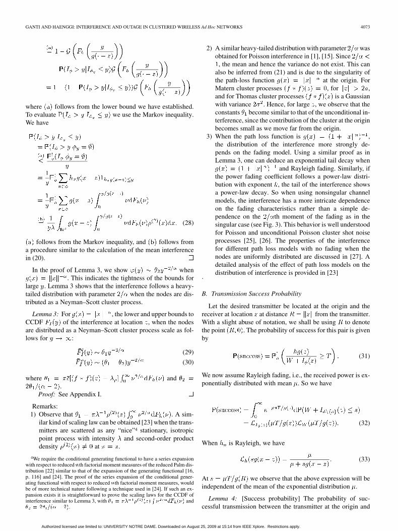
In the proof of Lemma 3, we show when. This indicates the tightness of the bounds for

large . Lemma 3 shows that the interference follows a heavy-tailed distribution with parameter when the nodes are dis-tributed as a Neyman–Scott cluster process.

Lemma 3: For , the lower and upper bounds toCCDF of the interference at location , when the nodesare distributed as a Neyman–Scott cluster process scale as fol-lows for :

(29)

(30)

where and.

Proof: See Appendix I.

Remarks:1) Observe that . A sim-

ilar kind of scaling law can be obtained [23] when the trans-mitters are scattered as any “nice”4 stationary, isotropicpoint process with intensity and second-order productdensity at .

4We require the conditional generating functional to have a series expansionwith respect to reduced �th factorial moment measures of the reduced Palm dis-tribution [22] similar to that of the expansion of the generating functional [16,p. 116] and [24]. The proof of the series expansion of the conditional gener-ating functional with respect to reduced �th factorial moment measures, wouldbe of more technical nature following a technique used in [24]. If such an ex-pansion exists it is straightforward to prove the scaling laws for the CCDF ofinterference similar to Lemma 3, with � � �� and� � �� .

2) A similar heavy-tailed distribution with parameter wasobtained for Poisson interference in [1], [15]. Since

, the mean and hence the variance do not exist. This canalso be inferred from (21) and is due to the singularity ofthe path-loss function at the origin. ForMatern cluster processes , for ,and for Thomas cluster processes is a Gaussianwith variance . Hence, for large , we observe that theconstants become similar to that of the unconditional in-terference, since the contribution of the cluster at the originbecomes small as we move far from the origin.

3) When the path loss function is ,the distribution of the interference more strongly de-pends on the fading model. Using a similar proof as inLemma 3, one can deduce an exponential tail decay when

and Rayleigh fading. Similarly, ifthe power fading coefficient follows a power-law distri-bution with exponent , the tail of the interference showsa power-law decay. So when using nonsingular channelmodels, the interference has a more intricate dependenceon the fading characteristics rather than a simple de-pendence on the th moment of the fading as in thesingular case (see Fig. 3). This behavior is well understoodfor Poisson and unconditional Poisson cluster shot noiseprocesses [25], [26]. The properties of the interferencefor different path loss models with no fading when thenodes are uniformly distributed are discussed in [27]. Adetailed analysis of the effect of path loss models on thedistribution of interference is provided in [23]

.

B. Transmission Success Probability

Let the desired transmitter be located at the origin and thereceiver at location at distance from the transmitter.With a slight abuse of notation, we shall be using to denotethe point . The probability of success for this pair is givenby

(31)

We now assume Rayleigh fading, i.e., the received power is ex-ponentially distributed with mean . So we have

(32)

When is Rayleigh, we have

(33)

At we observe that the above expression will beindependent of the mean of the exponential distribution .

Lemma 4: [Success probability] The probability of suc-cessful transmission between the transmitter at the origin and



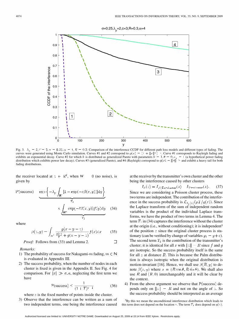
Fig. 3. � � �� : Comparison of the interference CCDF for different path loss models and different types of fading. Thecurves were generated using Monte Carlo simulation. Curves #1 and #2 correspond to �� . Curve #1 corresponds to Rayleigh fading andexhibits an exponential decay. Curve #2 for which is distributed as generalized Pareto with parameters � � � � � �� (a hypothetical power fadingdistribution which exhibits power law decay). Curves #3 (generalized Pareto), and #4 (Rayleigh) correspond to �� and exhibit a heavy tail for bothfading distributions.

the receiver located at , when (no noise), isgiven by

success

(34)

where

(35)

Proof: Follows from (33) and Lemma 2.

Remarks:1) The probability of success for Nakagami- fading,

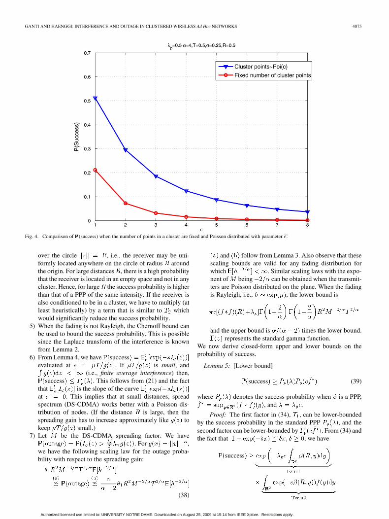
is evaluated in Appendix III.2) The success probability, when the number of nodes in each

cluster is fixed is given in the Appendix II. See Fig. 4 forcomparison. For , neglecting the first term wehave

success (36)

where is the fixed number of points inside the cluster.3) Observe that the interference can be written as a sum of

two independent terms, one being the interference caused

at the receiver by the transmitter’s own cluster and the otherbeing the interference caused by other clusters

(37)

Since we are considering a Poisson cluster process, thesetwo terms are independent. The contribution of the interfer-ence in the success probability is . Sincethe Laplace transform of the sum of independent randomvariables is the product of the individual Laplace trans-forms, we have the product of two terms in Lemma 4. Theterm in (34) captures the interference without the clusterat the origin (i.e., without conditioning); it is independent5

of the position since the original cluster process is sta-tionary (can be verified by change of variables ).The second term is the contribution of the transmitter’scluster; it is identical for all with since andare isotropic. So the success probability itself is the samefor all at distance . This is because the Palm distribu-tion is always isotropic when the original distribution ismotion-invariant [16]. Hence, we shall use to de-note where . We shall alsouse and interchangeably and it will be clear bythe context.

4) From the above argument we observe that success de-pends only on and not on the angle of . Sothe success probability should be interpreted as an average

5By this we mean the unconditional interference distribution which leads tothis term does not depend on the location . The term � does depend on �� .



Fig. 4. Comparison of (success) when the number of points in a cluster are fixed and Poisson distributed with parameter ��.

over the circle , i.e., the receiver may be uni-formly located anywhere on the circle of radius aroundthe origin. For large distances , there is a high probabilitythat the receiver is located in an empty space and not in anycluster. Hence, for large the success probability is higherthan that of a PPP of the same intensity. If the receiver isalso conditioned to be in a cluster, we have to multiply (atleast heuristically) by a term that is similar to whichwould significantly reduce the success probability.

5) When the fading is not Rayleigh, the Chernoff bound canbe used to bound the success probability. This is possiblesince the Laplace transform of the interference is knownfrom Lemma 2.

6) From Lemma 4, we have successevaluated at . If is small, and

(i.e., finite average interference) then,success . This follows from (21) and the fact

that is the slope of the curveat . This implies that at small distances, spreadspectrum (DS-CDMA) works better with a Poisson dis-tribution of nodes. (If the distance is large, then thespreading gain has to increase approximately like tokeep small.)

7) Let be the DS-CDMA spreading factor. We have. For ,

we have the following scaling law for the outage proba-bility with respect to the spreading gain:

(38)

and follow from Lemma 3. Also observe that thesescaling bounds are valid for any fading distribution forwhich . Similar scaling laws with the expo-nent of being can be obtained when the transmit-ters are Poisson distributed on the plane. When the fadingis Rayleigh, i.e., , the lower bound is

and the upper bound is times the lower bound.represents the standard gamma function.

We now derive closed-form upper and lower bounds on theprobability of success.

Lemma 5: [Lower bound]

success (39)

where denotes the success probability when is a PPP,, and .

Proof: The first factor in (34), , can be lower-boundedby the success probability in the standard PPP , and thesecond factor can be lower-bounded by . From (34) andthe fact that , we have

success



follows from change of variables, interchanging integrals,and using .

Since is convex and , UsingJensen’s inequality we have

Changing variables and using , we get

Hence

Since , by Young’s inequality [28] we have, where (conjugate exponents). For

(Matern) and (Thomas), we getsuccess . In general, ,

which is for Matern and for Thomas processes.In the latter case, when is Gaussian, is also Gaussianwith variance , hence . From [9], we get (bychange of variables)

(40)

We have• for ,

where

see [9];• for

Let and. By Hölder’s inequality we have

. Also, let .

Lemma 6: [Upper bound]

success

Proof: Neglecting the second term and using, we have

From the above two lemmas, we get

success

from which follows success as as ex-pected. In Lemma 6, we have neglected the contribution of thetransmitter’s cluster. We derive the following upper bound inthe proof of Lemma 8:

success (41)

where . Substituting for , wehave

success

(42)

Expression (42) is a tighter bound than the bound in Lemma 6,but not easily computable due to the presence of (for a given

and and are constants). In (42), the outage dueto the interference by the transmitting cluster is also taken intoaccount.

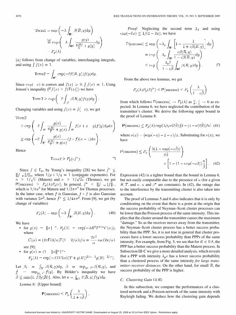
The proof of Lemmas 5 and 6 also indicates that it is only byconditioning on the event that there is a point at the origin thatthe success probability of Neyman–Scott cluster processes canbe lower than the Poisson process of the same intensity. This im-plies that the cluster around the transmitter causes the maximum“damage.” So as the receiver moves away from the transmitter,the Neyman–Scott cluster process has a better success proba-bility than the PPP. So, it is not true in general that cluster pro-cesses have a lower success probability than PPPs of the sameintensity. For example, from Fig. 5, we see that for , thePPP has a better success probability than the Matern process. InSubsection III-C we give a more detailed analysis, which revealsthat a PPP with intensity has a lower success probabilitythan a clustered process of the same intensity for large trans-mitter–receiver distances. On the other hand, for small , thesuccess probability of the PPP is higher.

C. Clustering Gain

In this subsection, we compare the performances of a clus-tered network and a Poisson network of the same intensity withRayleigh fading. We deduce how the clustering gain depends



Fig. 5. Comparison of success probability for cluster and Poisson point processes.

on the transmitter–receiver distance. We use the followingnotation:

So success . is the probability ofsuccess due to the presence of the cluster at the origin near thetransmitter. is the probability of success in the presence ofother clusters. Interference from these other clusters contributesmore to the outage when is large. This is also intuitive, sinceas the receiver moves away from the transmitting cluster, theinterference from the other clusters starts to dominate. We definethe clustering gain as

The fluctuation of around unity indicates the existence ofa crossover point below which the PPP performs better thanclustered process and vice versa. So it is beneficial to inducelogical clustering of transmitters by MAC if .

We now consider for large , i.e., . Bythe dominated convergence theorem and (1), we have

(43)

Also from the derivation of upper bound we have. Hence, from the definition of

we have, . Hence, for large

(44)

So for large , most of the damage is done by transmitting nodesother than the cluster in which the intended transmitter lies.

Lemma 7:

(45)

Proof: See Appendix IV

Hence, for large

From (43) we have , for large, i.e., for large transmit–receive distance. We have

. Hence, the Poisson point process with in-tensity , has a lower success probability than the clusteredprocess of the same intensity for large transmit–receiver dis-tances.

For small depends on the behavior of the path lossfunction at . We consider the two cases when thechannel function is singular at the origin or not.

1) : In this case, we observe that. But at small is less than . We have the

following lemma.



Lemma 8: If for small and, then for small

success (46)

Proof: See Appendix V.

Note that for Matern and Thomas cluster process havethe required property. Hence, when , the PPPwith intensity has a higher success probability than the clus-tered process of the same intensity for small transmit–receiverdistance. Lemma 8 and the fact that also indicatethe existence of a crossover point between the success curvesof the PPP and the cluster process. So it is not true in generalthat the performance of the clustered process is better or worsethan that of the Poisson process. This is because, for the sameintensity, a clustered process will have clusters of transmitters(where interference is high) and also vacant areas (where thereare no transmitters and interference is low), whereas in a Poissonprocess, the transmitters are uniformly spread.

2) : can be written as

Hence, can also be written as follows:

(47)

where , with. Observe that . If the total den-

sity of the transmitters is fixed, i.e., is constant, howdoes behave with respect to ? We have the followinglemma which characterizes the monotonicity of with re-spect to .

Lemma 9: Given is constant, is decreasingwith , i.e., iff , where

Proof: From (47)

We have

and is decreasing in

where is given by

Since is decreasing in , we have that isdecreasing in . So a necessary and sufficient condition for

is . We want

(48)

Observations:1) Since , we have that is increasing with

(like , and hence will be greater than at somefor a fixed .

2) We have and specifically at.

3) From Lemma 9 and Remark 2, we can deduceif , i.e., the gain decreases

from with increasing if the total intensity of transmittersis less than .

4) Since is continuous with respect to is closeto for small .

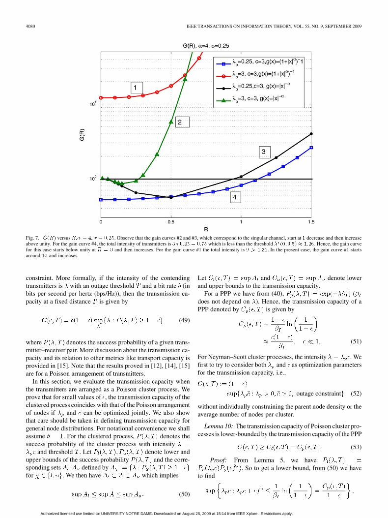
5) From Fig. 7, we observe that increases monotoni-cally with .

In Fig. 6, is plotted against . The term inthe gain represents the effect of the interference caused byother clusters on the relative gain. If we suppose that the trans-mitter was not a part of the process , then the termwould vanish. So in this case the probability of success in theclustering case is given by . Lemma 5 would implya gain greater than unity. This is intuitive because clustering ofthe transmitters would reduce the chance of an interfering trans-mitter being near the intended receiver. So it is the interferencefrom the transmitter’s own cluster which makes the relative gainsmaller or larger than unity.

We provide some heuristics as to when logical clustering doesnot perform better than a uniform distribution of points.

• The exact value of at which crosses is diffi-cult to find analytically due to the highly nonlinear natureof . If such a crossover point exists (depends on thepath-loss model) we will denote it by .



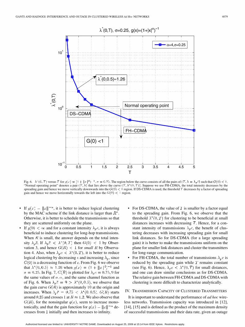
Fig. 6. � �� versus � for �� . The region below the curve consists of all the pairs of �� such that �� .“Normal operating point” denotes a pair �� that lies above the curve �� . Suppose we use FH-CDMA, the total intensity decreases by thespreading gain and hence we move vertically downwards into the �� region. If DS-CDMA is used, the threshold � decreases by a factor of spreadinggain and hence we move horizontally towards the left into the �� region.

• If , it is better to induce logical clusteringby the MAC scheme if the link distance is larger than .Otherwise, it is better to schedule the transmissions so thatthey are scattered uniformly on the plane.

• If and for a constant intensity , it is alwaysbeneficial to induce clustering for long-hop transmissions.When is small, the answer depends on the total inten-sity . If then by Obser-vation 3, and hence for small by Observa-tion 4. Also, when , it is better to reducelogical clustering by decreasing and increasing , since

is a decreasing function of . From Fig. 6 we observethat when and

. In Fig. 7, is plotted for forthe same values of and the same channel function asof Fig. 6. When , we observe thatthe gain curve is approximately at the origin andincreases. When startsaround and crosses at . We also observe that

, for the nonsingular , seem to increase mono-tonically, and that the gain function for de-creases from initially and then increases to infinity.

• For DS-CDMA, the value of is smaller by a factor equalto the spreading gain. From Fig. 6, we observe that thethreshold for clustering to be beneficial at smalldistances increases with decreasing . Hence, for a con-stant intensity of transmissions , the benefit of clus-tering decreases with increasing spreading gain for smalllink distances. So for DS-CDMA (for a large spreadinggain) it is better to make the transmissions uniform on theplane for smaller link distances and cluster the transmittersfor long-range communication.

• For FH-CDMA, the total number of transmissions isreduced by the spreading gain while remains constant(see Fig. 6). Hence, for small distances,and one can draw similar conclusions as for DS-CDMA.The relative gain between FH-CDMA and DS-CDMA withclustering is more difficult to characterize analytically.

IV. TRANSMISSION CAPACITY OF CLUSTERED TRANSMITTERS

It is important to understand the performance of ad hoc wire-less networks. Transmission capacity was introduced in [12],[14], [15] and is defined as the product of the maximum densityof successful transmissions and their data rate, given an outage



Fig. 7. �� versus �� . Observe that the gain curves #2 and #3, which correspond to the singular channel, start at � decrease and then increaseabove unity. For the gain curve #4, the total intensity of transmitters is � �� which is less than the threshold � �� . Hence, the gain curvefor this case starts below unity at � � � and then increases. For the gain curve #1 the total intensity is � � ��. In the present case, the gain curve #1 startsaround �� and increases.

constraint. More formally, if the intensity of the contendingtransmitters is with an outage threshold and a bit rate (inbits per second per hertz (bps/Hz)), then the transmission ca-pacity at a fixed distance is given by

(49)

where denotes the success probability of a given trans-mitter–receiver pair. More discussion about the transmission ca-pacity and its relation to other metrics like transport capacity isprovided in [15]. Note that the results proved in [12], [14], [15]are for a Poisson arrangement of transmitters.

In this section, we evaluate the transmission capacity whenthe transmitters are arranged as a Poisson cluster process. Weprove that for small values of , the transmission capacity of theclustered process coincides with that of the Poisson arrangementof nodes if and can be optimized jointly. We also showthat care should be taken in defining transmission capacity forgeneral node distributions. For notational convenience we shallassume . For the clustered process, denotes thesuccess probability of the cluster process with intensity

and threshold . Let denote lower andupper bounds of the success probability and the corre-sponding sets defined byfor . We then have which implies

(50)

Let and denote lowerand upper bounds to the transmission capacity.

For a PPP we have from (40), (does not depend on ). Hence, the transmission capacity of aPPP denoted by is given by

(51)

For Neyman–Scott cluster processes, the intensity . Wefirst to try to consider both and as optimization parametersfor the transmission capacity, i.e.,

outage constraint (52)

without individually constraining the parent node density or theaverage number of nodes per cluster.

Lemma 10: The transmission capacity of Poisson cluster pro-cesses is lower-bounded by the transmission capacity of the PPP

(53)

Proof: From Lemma 5, we have. So to get a lower bound, from (50) we have

to find



This maximum value of is attained when , while, such that . So we have

.

Also observe that and . This correspondsto the scenario in which the clustered process degenerates to aPPP. We also have the following upper bound.

Lemma 11: Let with .For , we have

(54)

Proof: See Appendix VI.

Theorem 2: For we have .Proof: Follows from the Lemmas 10 and 11.

From the above two proofs, when is small, the transmissioncapacity is equal to the Poisson process of same intensity. Thiscapacity is achieved when and . This is thescenario in which the cluster process becomes a PPP. This isdue to the definition of the transmission capacity as

outage constraint where we havetwo variables to optimize over.

Instead, we may fix and find the transmission capacity withrespect to . So we define constrained transmission capacity as

outage constraint

We have the following bounds for .

Theorem 3:

Proof: From the lower bound on success

lower bounds outage constraint . So we have.

Similary, from the upper bound on success

upper-bounds outage constraint .

One can also derive an order approximation to the constrainedtransmission capacity when is very small. We have the fol-lowing order approximation to transmission capacity.

Proposition 1: When is fixed, the constrained transmis-sion capacity is given by

(55)

when .Proof: Let denote the outage probability, i.e.,

We have , which implies is increasing andinvertible and hence . We approx-imate for small by the Lagrange inversion theorem.Observe that is a smooth function of and all derivativesexist. Expanding around by the Lagrange inver-sion theorem and using yields

(56)

where follows by applying de L’Hôpital’s rule.

We have the following observations.1) The constrained transmission capacity increases (slowly)

with .2) We also observe that the constrained transmission capacity

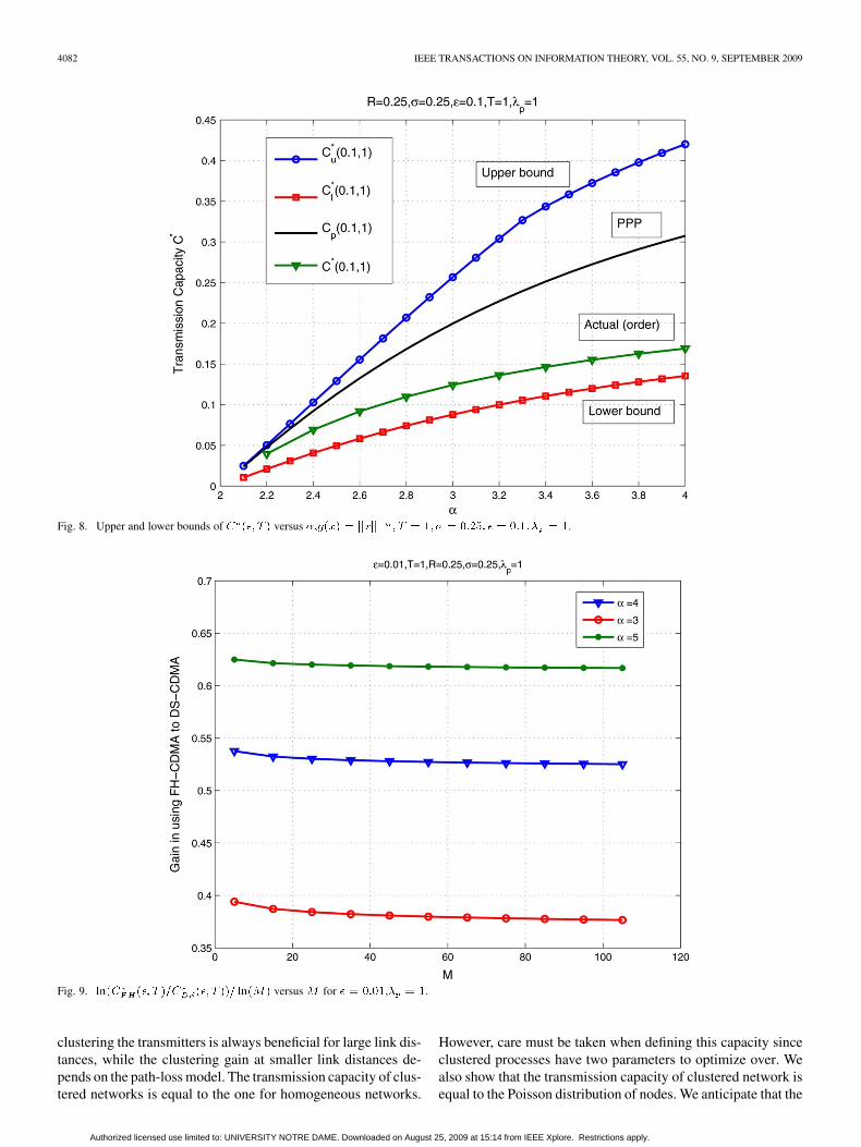
for the cluster process is always less than that of a Poissonnetwork (see Fig. 8) and approaches as .

3) When FH-CDMA with intracluster frequency hopping isutilized, we have the cluster intensity reduced by a factor

(spreading gain). One can easily obtain the constrainedtransmission capacity of this system to be

When DS-CDMA is used, the constrained transmission ca-pacity is . When the transmit-ters are spread as a Poisson point process, we have from[29], [30]

In Fig. 9, we plot withrespect to spreading gain , when the path loss functionis and . From the figure, we ob-serve a similar gain, even in the case of clusteredtransmitters.

V. CONCLUSION

Previous work characterizing interference, outage, and trans-mission capacity in large random networks exclusively focusedon the homogeneous PPP as the underlying node distribution. Inthis paper, we extend these results to clustered processes. Clus-tering may be geographical, i.e., given by the spatial distributionof the nodes, or it may be induced logically by the MAC scheme.We use tools from stochastic geometry and Palm probabilitiesto obtain the conditional Laplace transform of the interference.Upper and lower bounds are obtained for the CCDF of the inter-ference for any stationary distribution of nodes and fading. Wehave shown that the distribution of interference depends heavilyon the path-loss model considered. In particular, the existence ofa singularity in the model greatly affects the results. This con-ditional Laplace transform is used to obtain the probability ofsuccess in a clustered network with Rayleigh fading. We show



Fig. 8. Upper and lower bounds of � �� versus �� .

Fig. 9. �� versus � for � � ��, � �.

clustering the transmitters is always beneficial for large link dis-tances, while the clustering gain at smaller link distances de-pends on the path-loss model. The transmission capacity of clus-tered networks is equal to the one for homogeneous networks.

However, care must be taken when defining this capacity sinceclustered processes have two parameters to optimize over. Wealso show that the transmission capacity of clustered network isequal to the Poisson distribution of nodes. We anticipate that the



analytical techniques used in this work will be useful for otherproblems as well. In particular, the conditional generating func-tionals are likely to find wide applicability.

APPENDIX IPROOF OF LEMMA 3

Proof: We first evaluate the asymptotic behavior of. Let . We have

where follows from the fact thatfor close to and for large . By a similar ex-pansion of , (57), and the dominated convergence theorem,we have

(57)

By change of variables and using[28, p. 198], we have

We similarly have

(58)

where follows from the Lebesgue dominated convergencetheorem ( is a very nice function since is a probability den-sity function (PDF)). So we have .For a Neyman–Scott cluster process, the second-order productdensity is given by [16, p. 158]

where is the distribution of the number of points in therepresentative cluster. denotes the density of the dis-

tribution function for the distance between two independentrandom points which were scattered using the distribution

of the representative cluster. When the number of pointsinside each cluster is Poisson distributed with mean , we have

. We also have .Estimating we have

(59)

By change of variables, we have

(60)

For the term

(61)

So we have . Hence, from Theorem 1, we haveand .

APPENDIX IIOUTAGE PROBABILITY IN POISSON CLUSTER PROCESS WHEN

THE NUMBER OF CLUSTER POINTS ARE FIXED

In this appendix, we derive the conditional Laplace transformin a Poisson cluster process, when the number of points in eachcluster is fixed to be and . We also assume thateach point is independently distributed with density . In thiscase, the moment generating function of the number of pointsin the representative cluster is given by

Using the same notation as in Section II-B, and from (11) and(13), we have



where follows from the fact that the points are independentlydistributed and we are not counting the point at the origin. In thiscase, is given by

Hence, the success probability (Rayleigh fading) is given by

success

where

APPENDIX IIIOUTAGE PROBABILITY OF NAKAGAMI- FADING

Here, we derive the success probability when the fading dis-tribution is Nakagami- distributed. We also assumeand . The PDF of the power fading coefficient isgiven by

From (34), we have

success

Using integration by parts we get

success

(62)

where follows from the series expansion of incompleteGamma function when is an integer and follows from

the properties of the Laplace transform andwhen is an integer. We also have

Hence, from Lemma 2, we have

(63)

where

For integer success can be evaluated from (62) and(63). For , the probability evaluated from (62) and (63)matches that of Lemma 4.

APPENDIX IVPROOF OF LEMMA 7

Proof:

which is equal to

Since , we have that . We alsohave from the dominated convergence theorem and (1)

which is a constant. So using Fatou’s lemma [28], we have

APPENDIX VPROOF OF LEMMA 8

Proof: From (47), the probability of success is

success



where

and

an increasing function of . From Young’s inequality [28, Sec.8.7] we haveHence

With a slight abuse of notation, let

Hence

(64)

Also observe that . So .

If one considers and as identical and independentrandom variables with density functions , we then have

. Let be

some constant. Using the Chebyshev inequality we get

(**)

The PDF of is given by , since is rotation-invariant. Choosing we have

(**)

(65)

So we have

(66)

Also we have . So we havefor small . Hence

for small we have success .

APPENDIX VIPROOF OF LEMMA 11

Proof: We have from the derivation of Lemma 8

(67)

where . With, it is sufficient to prove

. Also, observe that asindependent of . Hence, we can assume is finite for theproof. We proceed by contradiction.

Let . Hence, there exists asuch that . At this

value of we have

(68)

From the derivation of Lemma 8, we have, with equality only when . Hence, we

have

(69)

Since , we have .Using the upper bound for , we find

(70)

Using the inequality ,substituting , we get . Hence,we have

(71)



So if , and finite, we also have .So we have a contradiction from (68) and (71). Hence, thereexists no such and hence . We can achieve

, by usingfor very large. As .

REFERENCES

[1] E. S. Sousa and J. A. Silvester, “Optimum transmission ranges in a di-rect-sequence spread spectrum multihop packet radio network,” IEEEJ. Sel. Areas Commun., vol. 8, no. 5, pp. 762–771, Jun. 1990.

[2] R. Mathar and J. Mattfeldt, “On the distribution of cumulated interfer-ence power in Rayleigh fading channels,” Wireless Netw., vol. 1, no. 1,pp. 31–36, 1995.

[3] M. Westcott, “On the existence of a generalized shot-noise process,”in Studies in Probability and Statistics. Papers in Honour of EdwinJG Pitman. Amsterdam, The Netherlands: North-Holland, 1976, p.7388.

[4] S. O. Rice, “Mathematical analysis of random noise,” Bell Syst. Tech,J., 23, pp. 282–332, Jul., 1944.

[5] J. Rice, “On generalized shot noise,” Adv. Appl. Probab., vol. 9, no. 3,pp. 553–565, 1977.

[6] L. Heinrich and V. Schmidt, “Normal convergence of multidimen-sional shot noise and rates of this convergence,” Adv. Appl. Probab.,vol. 17, no. 4, pp. 709–730, 1985.

[7] J. Ilow and D. Hatzinakos, “Analytic alpha-stable noise modeling in aPoisson field of interferers or scatterers,” IEEE Trans, Signal Process.,vol. 46, no. 6, pp. 1601–1611, Jun. 1998.

[8] M. Shao and C. Nikias, “Signal processing with fractional lower ordermoments: Stable processes and their applications,” Proc. IEEE, vol. 81,no. 7, pp. 986–1010, Jul. 1993.

[9] F. Baccelli, B. Blaszczyszyn, and P. Muhlethaler, “An Aloha protocolfor multihop mobile wireless networks,” IEEE Trans. Inf. Theory, no.2, pp. 421–426, Feb. 2006.

[10] J. Venkataraman and M. Haenggi, “Optimizing the throughput inrandom wireless ad hoc networks,” in Proc. 42nd Annu. Allerton Conf.Communication, Control, and Computing, Monticello, IL, Oct. 2004.

[11] J. Venkataraman, M. Haenggi, and O. Collins, “Shot noise models forthe dual problems of cooperative coverage and outage in random net-works,” in Proc. 44th Annu. Allerton Conf. Communication, Control,and Computing, Monticello, IL, Sep. 2006.

[12] S. Weber and J. G. Andrews, “A stochastic geometry approach to wide-band ad hoc networks with channel variations,” in Proc. 2nd Workshopon Spatial Stochastic Models for Wireless Networks, Boston, MA, Apr.2006, pp. 1–6.

[13] M. Haenggi, “Outage and throughput bounds for stochastic wirelessnetworks,” in Proc. IEEE Int. Symp. Information Theory, , Adelaida,Australia, Sep. 2005, pp. 2070–2074.

[14] S. Weber, X. Yang, J. Andrews, and G. de Veciana, “Transmissioncapacity of wireless ad hoc networks with outage constraints,” IEEETrans. Inf. Theory, vol. 51, no. 12, pp. 4091–4102, Dec. 2005.

[15] S. Weber and J. G. Andrews, “Bounds on the SIR distribution for aclass of channel models in ad hoc networks,” in Proc. 49th Annu. IEEEGlobecom Conf., San Francisco, CA, Nov. 2006, pp. 1–5.

[16] D. Stoyan, W. S. Kendall, and J. Mecke, Stochastic Geometry and itsApplications, ser. Wiley Series in Probability and Mathematical Statis-tics, 2nd ed. New York: Wiley, 1995.

[17] O. Kallenberg, Random Measures. Berlin, Germany: Akademie-Verlag, 1983.

[18] D. J. Daley and D. Vere-Jones, An Introduction to the Theory of PointProcesses, 2nd ed. New York: Springer, 1998.

[19] D. R. Cox and V. Isham, Point Processes. London/New York:Chapman & Hall, 1980.

[20] L. Heinrich, “Asymptotic behaviour of an emperical nearest-neigh-bour distance function for stationary Poisson cluster processes,” Math.Nachr., vol. 136, pp. 131–148, 1988.

[21] M. Baudin, “Likelihood and nearest-neighbor distance properties ofmultidimensional poisson cluster processes,” J. Appl. Probab., vol. 18,no. 4, pp. 879–888, 1981.

[22] K. H. Hanisch, “Reduction of the n-th moment measures and the spe-cial case of the third moment measure of stationary and isotropic planarpoint process,” Mathematische Operationsforschung and Statistik (Se-ries Statistics), vol. 14, pp. 421–435, 1983.

[23] R. Ganti and M. Haenggi, “Interference in ad hoc networks with gen-eral motion-invariant node distributions,” in Proc. IEEE Int. Symp. In-formation Theory , Toronto, ON, Canada, Jul. 2008, pp. 1–5.

[24] M. Westcott, “The probability generating functional,” J. AustralianMath. Soc., vol. 14, pp. 448–466, 1972.

[25] S. Lowen and M. Teich, “Power-law shot noise,” IEEE Trans. Inf.Theory,, vol. 36, no. 6, pp. 1302–1318, Nov. 1990.

[26] G. Samorodnitsky, “Tail Behavior of Shot Noise Processes,” [Online].Available: http://citeseer.ist.psu.edu/603758.html

[27] H. Inaltekin and S. Wicker, “The behavior of unbounded path-lossmodels and the effect of singularity on computed network interfer-ence.,” in Proc. 4th Annu. IEEE Comm. Soc. Conf. Sensor, Mesh andAd Hoc Communications and Networks SECON 2007, June 2007, pp.431–440.

[28] G. B. Folland, Real Analysis, Modern Techniques and Their Applica-tions, 2nd ed. New York: Wiley, 1999.

[29] J. Andrews, S. Weber, and M. Haenggi, “Ad hoc networks: To spreador not to spread?,” IEEE Commun. Mag., vol. 45, no. 12, pp. 84–91,Dec. 2007.

[30] S. Weber, J. Andrews, X. Yang, and G. de Veciana, “Transmission ca-pacity of wireless ad hoc networks with successive interference cancel-lation,” IEEE Trans. Inf. Theory, vol. 53, no. 8, pp. 2799–2814, Aug.2007.

Radha Krishna Ganti (S’01) received the B.Tech. and M.Tech. degrees in elec-trical engineering from Indian Institute of Technology, Madras, India, in 2004.

He is currently working towards the Ph.D. degree at the University of NotreDame, Notre Dame, IN.

Martin Haenggi (S’95–M’99–SM’04) received the Dipl. Ing. (M.Sc.) andPh.D. degrees in electrical engineering from the Swiss Federal Institute ofTechnology, Zurich (ETHZ) in 1995 and 1999, respectively.

After a postdoctoral year at the Electronics Research Laboratory at theUniversity of California, Berkeley, he joined the faculty of the ElectricalEngineering Department at the University of Notre Dame, Notre Dame, IN,in 2001, and is now an Associate Professor of Electrical Engineering there.During 2007–2008, he spent a sabbatical year at the University of California,San Diego (UCSD). His scientific interests include networking and wirelesscommunications, with an emphasis on ad hoc and sensor networks.

Prof. Haenggi is a Senior Member of the ACM. For both his M.Sc. and hisPh.D. theses, he was awarded the ETH medal, and he received a CAREER awardfrom the U.S. National Science Foundation in 2005. He served as a member ofthe Editorial Board of the Elsevier Journal of Ad Hoc Networks from 2005 to2008 and as a Distinguished Lecturer for the IEEE Circuits and Systems Societyin 2005–2006. Presently, he is an Associate Editor the IEEE TRANSACTIONS ON

MOBILE COMPUTING and the ACM Transactions on Sensor Networks.


Documents

IEEE TRANSACTIONS ON INFORMATION THEORY, VOL. 55, NO. 9, SEPTEMBER