IEEE TRANSACTIONS ON IMAGE PROCESSING, VOL. …library.utia.cas.cz/separaty/2017/ZOI/kotera-0474858.pdf · Blind Deconvolution With Model Discrepancies Jan Kotera, Student Member,

IEEE TRANSACTIONS ON IMAGE PROCESSING, VOL. 26, NO. 5, MAY 2017 2533

Blind Deconvolution With Model DiscrepanciesJan Kotera, Student Member, IEEE, Václav Šmídl, Member, IEEE, and Filip Šroubek, Member, IEEE

Abstract— Blind deconvolution is a strongly ill-posed problemcomprising of simultaneous blur and image estimation. Recentadvances in prior modeling and/or inference methodology led tomethods that started to perform reasonably well in real cases.However, as we show here, they tend to fail if the convolutionmodel is violated even in a small part of the image. Methodsbased on variational Bayesian inference play a prominent role.In this paper, we use this inference in combination with thesame prior for noise, image, and blur that belongs to the familyof independent non-identical Gaussian distributions, known asthe automatic relevance determination prior. We identify severalimportant properties of this prior useful in blind deconvolution,namely, enforcing non-negativity of the blur kernel, favoringsharp images over blurred ones, and most importantly, handlingnon-Gaussian noise, which, as we demonstrate, is common inreal scenarios. The presented method handles discrepancies inthe convolution model, and thus extends applicability of blinddeconvolution to real scenarios, such as photos blurred by cameramotion and incorrect focus.

Index Terms— Blind deconvolution, variational bayes, auto-matic relevance determination, gaussian scale mixture.

I. INTRODUCTION

NUMEROUS measuring processes in real world are mod-eled by convolution. The linear operation of convolution

is characterized by a convolution (blur) kernel, which isalso called a point spread function (PSF), since the kernelis equivalent to an image the device would acquire aftermeasuring an ideal point source (delta function). In deviceswith classical optical systems, such as digital cameras, opticalmicroscopes or telescopes, image blur caused by cameralenses or camera motion is modeled by convolution. Mediaturbulence (e.g. atmosphere in the case of terrestrial tele-scopes) generates blurring that is also modeled by convolution.In atomic force microscopy or scanning tunneling microscopy,resulting images are convolved with a PSF, whose shapeis related to the measuring tip shape. In medical imaging,e.g. magnetic resonance perfusion, pharmacokinetic modelsconsist of convolution with an unknown arterial input function.These are just a few examples of acquisition processes with aconvolution model. In many practical applications convolutionkernels are unknown. Then the problem of estimating latent

Manuscript received August 19, 2016; revised January 14, 2017 andFebruary 21, 2017; accepted February 21, 2017. Date of publicationMarch 1, 2017; date of current version April 1, 2017. This work wassupported by the Czech Science Foundation under Grant GA13-29225S andGrant GA15-16928S. The associate editor coordinating the review of thismanuscript and approving it for publication was Dr. Javier Mateos.

The authors are with the Institute of Information Theory and Automation,Czech Academy of Sciences, 182 08 Prague, Czech Republic (e-mail:[email protected]).

Color versions of one or more of the figures in this paper are availableonline at http://ieeexplore.ieee.org.

Digital Object Identifier 10.1109/TIP.2017.2676981

data from blurred observations without any knowledge ofkernels is called blind deconvolution.

Due to widespread presence of convolution in images, blinddeconvolution is an active field of research in image processingand computer vision. However, the convolution model may nothold over the whole image. Various optical aberrations alterimages so that only the central part of images follows theconvolution model. Physical phenomena such as occlusion,under and overexposure, violate the convolution model locally.It is therefore important to have a methodology that handlessuch discrepancies in the convolution model automatically.

Let us assume the standard image acquisition model, inwhich a noisy observed image g is a result of convolutionof a latent image u and an unknown PSF h, plus corruptionby noise ε,

g = h ∗ u + ε. (1)

The goal of blind image deconvolution is to recover u solelyfrom the given blurry image g.

We follow the stochastic approach and all the variablesin consideration are 2D random fields characterized by cor-responding probability distributions denoted as p(h), p(u),and p(ε). The Bayesian paradigm dictates that the infer-ence of u and h from the observed image g is done bymodeling the posterior probability distribution p(u, h|g) ∝p(g|u, h)p(u)p(h). Estimating the pair (u, h) is then accom-plished by maximizing the posterior p(u, h|g), which is com-monly referred to as maximum a posteriori (MAP) approach,sometimes denoted MAPu,h to emphasize the simultaneousestimation of image and blur. Levin et al. in [1] pointed outthat even for image priors p(u) that correctly capture natural-image statistics (sparse distribution of gradients), MAPu,h

approach tends to fail by returning a trivial “no-blur” solution,i.e., the estimated sharp image is equal to the input blurredinput g and the estimated blur is a delta function. However,MAPu,h avoids the “no-blur” solution if we artificially sparsifyintermediate images by shock filtering, removing weak edges,overestimating noise levels, etc., as widely used in [2]–[8].

From the Bayesian perspective, a more appropriate approachto blur kernel estimation is by maximizing the poste-rior marginalized w.r.t. the latent image u, i.e. p(h|g) =∫

p(u, h|g)du. This distribution can be expressed in closedform only for simple image priors (e.g. Gaussian) and suitableapproximation is necessary in other cases. In the Varia-tional Bayesian (VB) inference, we approximate the poste-rior p(u, h|g) by a restricted parametrization in factorizedform and optimize its Kullback-Leibler divergence to thecorrect solution. The optimization is tractable and the resultingapproximation provides an estimate of the sought marginaldistribution p(h|g).

1057-7149 © 2017 IEEE. Personal use is permitted, but republication/redistribution requires IEEE permission.See http://www.ieee.org/publications_standards/publications/rights/index.html for more information.

2534 IEEE TRANSACTIONS ON IMAGE PROCESSING, VOL. 26, NO. 5, MAY 2017

As soon as the blur h is estimated, the problem of recoveringu becomes much easier. It can be usually determined bythe very same model, only now we maximize the posteriorp(u|g, h), or outsourced to any of the multitude of availablenon-blind deconvolution methods.

It is important to realize, that the error between the obser-vation and the model, ε = g − h ∗ u, may not always beof stochastic uncorrelated zero-mean Gaussian nature – thetrue noise. In real-world cases, the observation error comesfrom many sources, e.g. sensor saturation, dead pixels orblur space-variance (objects moving in the scene) to namea few. Vast majority of blind deconvolution methods donot take any extra measures to handle model violation andthe fragile nature of blind blur estimation typically causescomplete failure when more than just a few pixels do notfit the assumed model, which unfortunately happens all toooften. A non-identical Gaussian distribution with automaticallyestimated precision, which is called the Automatic RelevanceDetermination model (ARD) [9], is simple enough to becomputationally tractable in the VB inference and yet flexibleenough to handle model discrepancies far beyond the limitedscope of Gaussian noise.

In this work, we adopt the probabilistic model ofTzikas et al. [10], which is based solely on VB approximationof the posterior p(u, h) and which uses the same ARD modelfor all the priors p(u), p(h), and importantly also for thenoise distribution p(ε). Our main focus is to analyze propertiesof the VB-ARD model and to elaborate on details of itsimplementation in real world scenarios, which was not directlyconsidered in the original work of Tzikas. Specifically, wepropose several extensions: include global precision for thewhole image in the noise distribution p(ε) to decouple theGaussian and non-Gaussian part of noise, different approxima-tion of the blur covariance matrix, pyramid scheme for the blurestimation, and handling convolution boundary conditions.We demonstrate that VB-ARD with proposed extensions isrobust to outliers and in this respect outperforms by a widemargin state-of-the-art methods.

The rest of the paper is organized as follows. Sec. IIoverviews related work in blind deconvolution, ARD modelingand masking. Sec. III discusses the importance of modelingthe data error by ARD. Sec. IV presents the VB algorithm withARD priors. Experimental validation of robustness to modeldiscrepancies is given in Sec. V and Sec. VI concludes thiswork.

II. RELATED WORK

First blind deconvolution algorithms appeared in telecom-munication and signal processing in early 80’s [11]. For along time, the general belief was that blind deconvolutionwas not just impossible, but that it was hopelessly impossible.Proposed algorithms usually worked only for special cases,such as astronomical images with uniform (black) background,and their performance depended on initial estimates of PSF’s;see [12], [13]. Over the last decade, blind deconvolutionexperiences a renaissance. The key idea behind the new algo-rithms is to address the ill-posedness of blind deconvolution

by characterizing the prior p(u) using natural image statisticsand by a better choice of estimators. A major performanceleap was achieved in [14] and [15] by applying VB toapproximate the posterior p(u, h|g) by simpler distributions.Other authors [6], [16]–[19] stick to the alternating MAPu,h

approach, yet their methods converge to a correct solution byusing appropriate ad hoc steps. It was advocated in [1] thatmarginalizing the posterior with respect to the latent image u isa proper estimator of the PSF h. The marginalized probabilityp(h|g) can be expressed in a closed form only for simplepriors, otherwise approximation methods such as VB [20] orthe Laplace approximation [21] must be used. More recentlyin [4], [22], and [23], even better results were achieved whenthe model of natural image statistics was abandoned and priorsthat force unnaturally sparse distributions were used instead.Such priors belong to the category of strong Super-Gaussiandistributions [24]. A formal justification of unnaturally sparsedistributions was given in [25] together with a unifyingframework for the MAP and VB formulation. An overviewof state-of-the-art VB blind deconvolution methods can befound in [26].

The ARD model was originally proposed for neural net-works in [9]. Each input variable has its associated hyperpara-meter that controls magnitudes of weights on connections outof that input unit. The weights have then independent Gaussianprior distributions with variance given by the correspondinghyperparameter. This prior distribution is also known as thescale mixture of Gaussian [27]. It is slightly less general thanstrong Super-Gaussian distributions but its advantage is thatit is nicely tractable in the VB inference [22]. Distributionsof the ARD type have been successfully used in the contextof deconvolution as image or PSF priors [28]–[31], and lessfrequently also as a noise model [10], [32], [33].

A method of masking was originally proposed for handlingconvolution boundary conditions [34], however it can bealso used for model discrepancies in blind deconvolution asdiscussed in [35]. A binary mask defines regions where con-volution model holds. It allows for a very fast implementationusing Fourier transform, which renders the method applicableto large scale problems. However, the main drawback of thisapproach is that the areas with model discrepancies are notestimated automatically and must determined in advance byother means. Saturated pixels were considered in [36] usingthe EM algorithm but only for a non-blind scenario. Explicitlyaddressing the problem of outliers in blind deconvolution wasproposed in [2] using MAPu,h and automatically masking outregions where the convolution model is violated. Handlingsevere Gaussian noise was e.g. proposed in [5] by mitigatingnoise via projections.

III. AUTOMATIC RELEVANCE DETERMINATION

In the discrete domain, convolution is expressed as matrix-vector multiplication. Then according to (1) the data error εi

of the i -th pixel is

εi = gi − Hiu = gi − Ui h , i = 1, . . . , N , (2)

where H and U are convolution matrices performing con-volution with the blur and latent image, respectively, and h

KOTERA et al.: BLIND DECONVOLUTION WITH MODEL DISCREPANCIES 2535

and u are column vectors containing lexicographically orderedelements of the corresponding 2D random fields. N is thetotal number of pixels. Subscript i in vectors denotes the i -thelement and in matrices the i -th row. If the subscript is omittedthen we mean the whole vector (or matrix).

In the majority of blind deconvolution methods, the dataerror term is assumed to be i.i.d. zero-mean Gaussian withprecision α, i.e.

p(ε|α) =∏

i

N (εi |0, α−1) . (3)

Such assumption leads to the common �2 data term α2

∑i (gi −

Ui h)2. However as we demonstrate below, if this Gaussian-error assumption is slightly violated (e.g. by pixel saturation,model locally doesn’t hold, etc.), the �2 data term gives anincorrect solution. It is therefore desirable to model both theGaussian and non-Gaussian part of the error, for which theStudent’s t-distribution is a good choice, as it is essentiallya scaled mixture of Gaussians and also plays nicely with theVB framework. As demonstrated earlier for the autoregressivemodel in [32], we propose using a Gaussian distribution withpixel-dependent factors γi modulated by the overall noiseprecision α. The error model of ε is then defined as

p(ε|α, γ ) =∏

i

N(εi |0, (αγi )

−1)

, (4)

to which we refer as the ARD model with common precision.To draw a parallel to the classical formulation, the data termin this case takes the form α

2

∑i γi (gi − Ui h)2. The power

of this model lies in determining the precisions α and γi

automatically. This is covered in the following section, wherewe formulate the VB inference. For the current discussion, itsuffices to state that we need priors also on γ . Let G denotethe standard Gamma distribution, defined as G(ξ |a, b) =(1/�(a))baξa−1

i exp(−bξ). We define the γ prior as

p(γ |ν) =∏

i

G(γi |ν, ν). (5)

Marginalizing p(ε|α, γ )p(γ |ν) over γ gives us the Student’st-distribution with zero mean, precision α and degrees offreedom 2ν. From the above model it follows that the meanof γi is equal to a/b = ν/ν = 1. If ν becomes large thenG(γi |ν, ν) tends to the delta distribution at 1 and the errormodel will be just a Gaussian distribution. As ν decreases,tails decay more slowly and γi will be allowed to adjust andautomatically suppress outliers violating the acquisition model.

The conventional ARD model used e.g. in [10] is

p∗(ε|γ ) =∏

i

N(εi |0, γ −1

i

),

p∗(γi ) = G(γi |aγ , bγ ). (6)

The marginal distribution of this prior over γ is a Student’st-distribution with 2aγ degrees of freedom. It is possible tochoose the number of degrees of freedom as a priori known –a common approach is to choose aγ , bγ as small as possible,yielding Student’s t-prior with infinite variance. Estimation ofthe hyperparameters aγ , bγ via a numerical MAP method hasbeen proposed in [10].

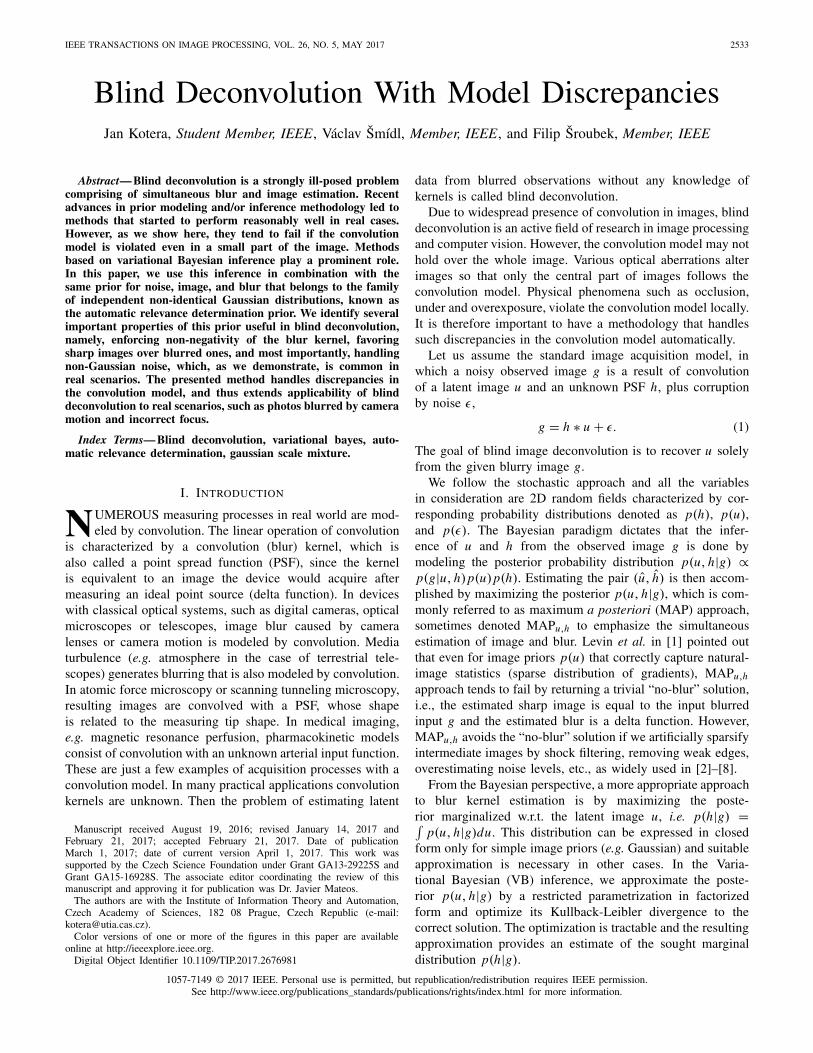
Fig. 1. Sharp (left) and intentionally blurred (right) image pair acquired foraccurate calculation of the blur PSF from the known patterns surrounding theimage.

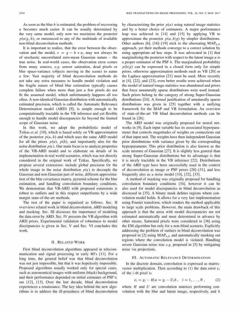
Fig. 2. Convolution error distribution in the case of real motion blur (solidgreen). It is much more heavy-tailed than the usually assumed Gaussian(dotted red, α = 0.6 · 103), while the Student’s t-distribution (dashed blue,2ν = 3.5, α = 1.2 · 105) is a perfect fit.

The ARD model is valuable in real scenarios even whenthere are no visible local discrepancies of the convolutionalmodel. We conjecture that under real image acquisition con-ditions there exists no convolution kernel h such that thedistribution of ε in (2) is strictly Gaussian. Different factorsinherently present in the acquisition process, such as lensimperfections, camera sensor discretization and quantization,contribute to the violation of the convolution model. To verifyour conjecture, we acquired several pairs of sharp–blurredimages (u, g) with intentional slight camera motion duringexposure. Except for this, we carefully avoided any otherkinds of error like pixel saturation or space-invariance of theblur and worked strictly with raw data from the camera. Foreach of these pairs we estimated the blur PSF h followingthe procedure suggested in [37], which uses patterns printedaround the image and designed to make the blur identificationstable; see example in Fig. 1. For this data, we measuredthe error of the convolution (2) and plotted its distribution(negative log) in Fig. 2. The distribution is far from Gaussian,as the maximum likelihood estimate of the Gaussian distrib-ution clearly provides a very poor approximation, especiallyin the tails. The Student’s t-distribution, on the other hand,approximates the error distribution correctly and thus justifiesthe ARD choice for p(ε). It is interesting to note, thatwe performed a similar analysis on Levin’s dataset [1] andobtained the same Student’s t-distribution of the convolutionerror. Another justification of the ARD model provided in [10]


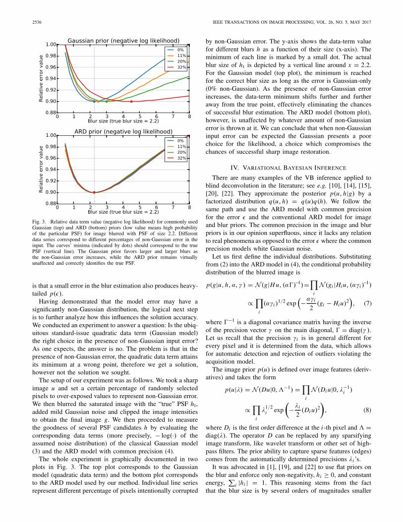
Fig. 3. Relative data term value (negative log likelihood) for commonly usedGaussian (top) and ARD (bottom) priors (low value means high probabilityof the particular PSF) for image blurred with PSF of size 2.2. Differentdata series correspond to different percentages of non-Gaussian error in theinput. The curves’ minima (indicated by dots) should correspond to the truePSF (vertical line). The Gaussian prior favors larger and larger blurs asthe non-Gaussian error increases, while the ARD prior remains virtuallyunaffected and correctly identifies the true PSF.

is that a small error in the blur estimation also produces heavy-tailed p(ε).

Having demonstrated that the model error may have asignificantly non-Gaussian distribution, the logical next stepis to further analyze how this influences the solution accuracy.We conducted an experiment to answer a question: Is the ubiq-uitous standard-issue quadratic data term (Gaussian model)the right choice in the presence of non-Gaussian input error?As one expects, the answer is no. The problem is that in thepresence of non-Gaussian error, the quadratic data term attainsits minimum at a wrong point, therefore we get a solution,however not the solution we sought.

The setup of our experiment was as follows. We took a sharpimage u and set a certain percentage of randomly selectedpixels to over-exposed values to represent non-Gaussian error.We then blurred the saturated image with the “true” PSF ht,added mild Gaussian noise and clipped the image intensitiesto obtain the final image g. We then proceeded to measurethe goodness of several PSF candidates h by evaluating thecorresponding data terms (more precisely, − log(·) of theassumed noise distribution) of the classical Gaussian model(3) and the ARD model with common precision (4).

The whole experiment is graphically documented in twoplots in Fig. 3. The top plot corresponds to the Gaussianmodel (quadratic data term) and the bottom plot correspondsto the ARD model used by our method. Individual line seriesrepresent different percentage of pixels intentionally corrupted

by non-Gaussian error. The y-axis shows the data-term valuefor different blurs h as a function of their size (x-axis). Theminimum of each line is marked by a small dot. The actualblur size of ht is depicted by a vertical line around x = 2.2.For the Gaussian model (top plot), the minimum is reachedfor the correct blur size as long as the error is Gaussian-only(0% non-Gaussian). As the presence of non-Gaussian errorincreases, the data-term minimum shifts further and furtheraway from the true point, effectively eliminating the chancesof successful blur estimation. The ARD model (bottom plot),however, is unaffected by whatever amount of non-Gaussianerror is thrown at it. We can conclude that when non-Gaussianinput error can be expected the Gaussian presents a poorchoice for the likelihood, a choice which compromises thechances of successful sharp image restoration.

IV. VARIATIONAL BAYESIAN INFERENCE

There are many examples of the VB inference applied toblind deconvolution in the literature; see e.g. [10], [14], [15],[20], [22]. They approximate the posterior p(u, h|g) by afactorized distribution q(u, h) = q(u)q(h). We follow thesame path and use the ARD model with common precisionfor the error ε and the conventional ARD model for imageand blur priors. The common precision in the image and blurpriors is in our opinion superfluous, since it lacks any relationto real phenomena as opposed to the error ε where the commonprecision models white Gaussian noise.

Let us first define the individual distributions. Substitutingfrom (2) into the ARD model in (4), the conditional probabilitydistribution of the blurred image is

p(g|u, h, α, γ ) = N (g|H u, (α�)−1)=∏

i

N (gi |Hiu, (αγi )−1)

∝∏

i

(αγi )1/2 exp

(−αγi

2(gi − Hiu)2

), (7)

where �−1 is a diagonal covariance matrix having the inverseof the precision vector γ on the main diagonal, � = diag(γ ).Let us recall that the precision γi is in general different forevery pixel and it is determined from the data, which allowsfor automatic detection and rejection of outliers violating theacquisition model.

The image prior p(u) is defined over image features (deriv-atives) and takes the form

p(u|λ) = N (Du|0,−1) =∏

i

N (Di u|0, λ−1i )

∝∏

i

λ1/2i exp

(

−λi

2(Di u)2

)

, (8)

where Di is the first order difference at the i -th pixel and =diag(λ). The operator D can be replaced by any sparsifyingimage transform, like wavelet transform or other set of high-pass filters. The prior ability to capture sparse features (edges)comes from the automatically determined precisions λi ’s.

It was advocated in [1], [19], and [22] to use flat priors onthe blur and enforce only non-negativity, hi ≥ 0, and constantenergy,

∑i |hi | = 1. This reasoning stems from the fact

that the blur size is by several orders of magnitudes smaller


than the image size and therefore inferring the blur from theposterior is driven primarily by the likelihood function (7) andless by the prior p(h). However, if the image estimation u isinaccurate, which is typically the case in the initial stages ofany blind deconvolution algorithm, then a more informativeprior p(h) is likely to help in avoiding local maxima and/orspeeding up the convergence. To keep the approach coherent,we apply the ARD model on blur intensities

p(h|β) = N (h|0, B−1) =∏

i

N (hi |0, β−1i )

∝∏

i

β1/2i exp

(

−βi

2h2

i

)

, (9)

where B = diag(β).The ARD models in (7), (8), and (9) are conditioned to

unknown precision parameters (α, γi , λi , βi ). The conjugatedistributions of precisions are Gamma distributions and thusfor image and blur precisions we have

p(λi ) = G(λi |aλ, bλ),

p(βi ) = G(βi |aβ, bβ) , (10)

and for the error precisions according to (4) and (5) we have

p(α) = G(α|aα, bα),

p(γi |ν) = G(γi |ν, ν) ,

p(ν) = G(ν|aν, bν). (11)

The hyperparameters a(·) and b(·) are user-defined constants.Let Z = {u, h, α, ν, {γi }, {λi }, {βi }} denote all the unknown

variables and Zk its particular member indexed by k. Usingthe above defined distributions, the posterior p(Z|g) is pro-portional to

p(g|u, h, α, γ )p(α)p(γ |ν)p(ν)p(u|λ)p(λ)p(h|β)p(β) .

The VB inference [38] approximates the posterior p(Z|g) bythe factorized distribution q(Z),

p(Z|g) ≈ q(Z) = q(u)q(h)q(α)q(ν)q(γ )q(λ)q(β). (12)

This is done by minimizing the Kullback-Leibler divergence,which provides a solution for individual factors

log q(Zk) ∝ El �=k[log p(Z|g)

], (13)

where El �=k denotes expectation with respect to all factorsq(Zl) except q(Zk). Formula (13) gives implicit solution,because each factor q(Zk) depends on moments of otherfactors. We must therefore resort to an iterative procedure andupdate the factors q in a loop.

A detailed derivation of update equations can be foundin [10] as the model is similar to ours. The interested reader isalso referred to [15] for better understanding of the derivation.In the following subsections we therefore only state the updateequations yet analyze their properties in detail.

A. Likelihood

The important feature is automatic estimation of the non-Gaussian part of the error modeled by precision γ . Utilizingthe combination of VB inference and ARD prior, we are ableto detect and effectively reject outliers from the estimation andachieve unprecedented robustness of the blur estimation, muchneeded in practical applications.

Using (13), q(γ ) becomes a Gamma distribution with amean value

γ i = 1 + 2 ν

α Eu,h[(gi − Hiu)2

] + 2 ν, (14)

where (·) denotes a mean value. Relating the inference to theclassical minimization of energy function − log p(u, h|g), theprecision γi corresponds to the weight of the i -th pixel indata fidelity term. The above equation shows that this weightis inversely proportional to the (expected) reconstruction errorat that pixel (up to the relaxation by ν/α) and it is updatedduring iterations, as the image and blur estimates change. Thistechnique is similar to the method of iteratively reweightedleast squares (IRLS), where the quadratic data terms arereweighted according to the error at the particular data pointto achieve greater robustness to outliers, but here it arisesnaturally as part of the VB framework. We demonstrate howthe method behaves with respect to outliers in the experimentalsection.

According to (14), the mean value of γ depends, apart fromu and h, only on the mean values α and ν. Using again theVB inference formula (13), one can deduce that both q(α) andq(ν) are Gamma distributions with mean values

α = N + 2aα∑N

i=1 γi Eu,h[(gi − Hiu)2

] + 2bα

(15)

and

ν = N + 2aν

2∑N

i=1(γi − Eγi

[log(γi )

] − 1) + 2bν

. (16)

The update equation of ν requires Stirling’s approximation; seee.g. [32] for detailed derivation. Note that the above updateequations (14), (15) and (16) are easy to compute.

Precision α is expected to be inversely proportional to thelevel of Gaussian noise in the input image. It is thereforeinteresting to observe how α behaves during iterations. Afterthe initialization, when the reconstruction error is high, theweight α is correspondingly low and thus the role of priors(regularization) is increased in the early stages of estimation.During subsequent iterations, as the estimation improves,α increases and the effect of priors is attenuated. It haslong been observed that this adjustment of data-term weightduring iterations is highly beneficial, if not necessary, for thesuccess of blind blur estimation, otherwise the optimizationtends to get stuck in a local minimum. Many state-of-the-art blind deconvolution methods therefore perform some kindof heuristic adjustment of the relative data-term/regularizerweight [7], often of the form of geometric progression αk+1 =rαk , where k denotes k-th iteration. The drawback of thisapproach is that the optimal constant r must be determinedby trial and error and, more importantly, the progression must


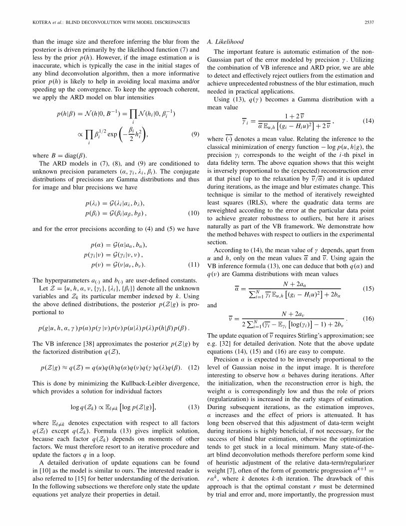
Fig. 4. Estimated noise precision as a function of iterations: The VariationalBayesian algorithm updates the noise precision in every iteration. The curvesdepict its typical development for different image SNRs; 50dB through 10dB.The diamond markers show the fixed update using geometric progressionαk = 1.5αk−1.

stop when the correct α (corresponding to the true noise level)is reached, which is not determined automatically but must bespecified by the user. The VB framework has an indisputableadvantage over more straightforward MAP methods – not onlydoes it give us the optimal update equation for the data-term precision, it also provides automatic saturation whenthe correct noise level is reached, as we can see in Fig. 4.During the early iterations the precision sharply increases andthen levels out at the correct value. For comparison we alsoshow the fixed geometric progression for r = 1.5 (diamondmarkers).

B. Image Prior

The factors associated with the image are q(u) and q(λ).Applying (13), we get (up to a constant)

log q(u)

= −Eh,α,γ,λ

[α(g−H u)T �(g−H u)+uT DT Du

], (17)

where the terms independent of u are omitted. The distributionq(u) is a normal distribution. The mean u and covariancecov(u) are obtained by taking the first and second orderderivatives of log(q(u)), respectively, and solving for zero.The update equation for the mean is a linear system

(Eh

[H T �H

]+ α−1 DT D

)u = H

T�g (18)

and for the covariance we get

cov u =(αEh

[H T �H

]+ DT D

)−1. (19)

The mean pixel precisions λi form the diagonal matrix .They are calculated from q(λ), which is a Gamma distributionwith the mean

λi = 1 + 2aλ

Eu[(Di u)2

] + 2bλ. (20)

The parameter bλ plays the role of relaxation, as it preventsdivision by zero in the case Di u = 0.

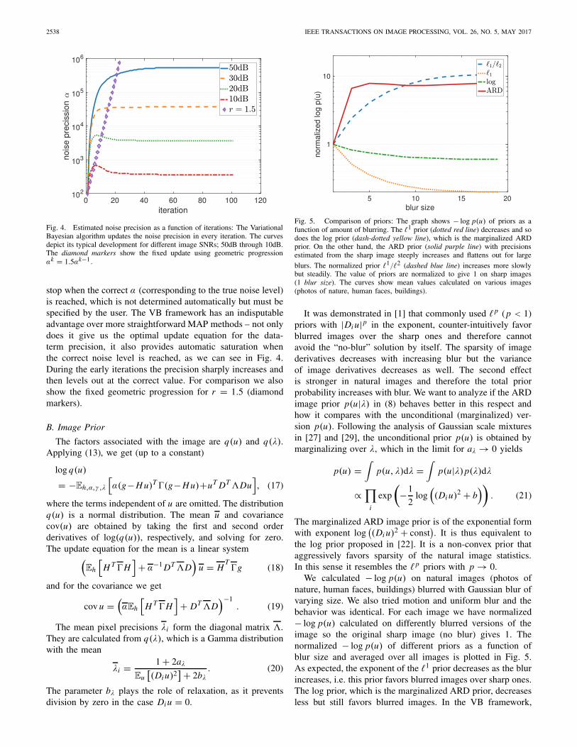
Fig. 5. Comparison of priors: The graph shows − log p(u) of priors as afunction of amount of blurring. The �1 prior (dotted red line) decreases and sodoes the log prior (dash-dotted yellow line), which is the marginalized ARDprior. On the other hand, the ARD prior (solid purple line) with precisionsestimated from the sharp image steeply increases and flattens out for large

blurs. The normalized prior �1/�2 (dashed blue line) increases more slowlybut steadily. The value of priors are normalized to give 1 on sharp images(1 blur size). The curves show mean values calculated on various images(photos of nature, human faces, buildings).

It was demonstrated in [1] that commonly used �p (p < 1)priors with |Di u|p in the exponent, counter-intuitively favorblurred images over the sharp ones and therefore cannotavoid the “no-blur” solution by itself. The sparsity of imagederivatives decreases with increasing blur but the varianceof image derivatives decreases as well. The second effectis stronger in natural images and therefore the total priorprobability increases with blur. We want to analyze if the ARDimage prior p(u|λ) in (8) behaves better in this respect andhow it compares with the unconditional (marginalized) ver-sion p(u). Following the analysis of Gaussian scale mixturesin [27] and [29], the unconditional prior p(u) is obtained bymarginalizing over λ, which in the limit for aλ → 0 yields

p(u) =∫

p(u, λ)dλ =∫

p(u|λ)p(λ)dλ

∝∏

i

exp

(

−1

2log

((Di u)2 + b

))

. (21)

The marginalized ARD image prior is of the exponential formwith exponent log

((Di u)2 + const

). It is thus equivalent to

the log prior proposed in [22]. It is a non-convex prior thataggressively favors sparsity of the natural image statistics.In this sense it resembles the �p priors with p → 0.

We calculated − log p(u) on natural images (photos ofnature, human faces, buildings) blurred with Gaussian blur ofvarying size. We also tried motion and uniform blur and thebehavior was identical. For each image we have normalized− log p(u) calculated on differently blurred versions of theimage so the original sharp image (no blur) gives 1. Thenormalized − log p(u) of different priors as a function ofblur size and averaged over all images is plotted in Fig. 5.As expected, the exponent of the �1 prior decreases as the blurincreases, i.e. this prior favors blurred images over sharp ones.The log prior, which is the marginalized ARD prior, decreasesless but still favors blurred images. In the VB framework,


however, we do not work with the marginalized ARD priorand instead iteratively estimate the prior precisions λi ’s fromthe current estimate of u using the update formula (20). Let usassume an ideal situation in which the precisions are estimatedfrom the sharp image, then the ARD prior shows correctbehavior similarly to the normalized prior �1/�2 [39] thatcompensates for the effect of decreasing image variance. Thisideal case is not achievable in practice, since we do not havea correct estimate of the sharp image u at the beginning, butit can be regarded as an upper bound. As the VB inferencemakes the approximation of the posterior more accurate withevery iteration, we approach this upper bound.

C. Blur Prior

As stated earlier, we use the same ARD model also forthe blur prior (9). Analogously to the derivation of the imagedistribution q(u) in (17), the form of blur factor q(h) is aGaussian distribution given by

log q(h) = −Eu,α,γ,β

[α(g − Uh)T �(g − Uh) + hT Bh

].

Then the mean h is the solution of the linear system(Eu

[U T �U

]+ α−1 B

)h = U

T�g (22)

and the covariance is

cov h =(αEu

[U T �U

]+ B

)−1. (23)

The distribution q(β) of the blur precision is again a Gammadistribution and for the mean values of βi we get analogouslyto (20)

β i = 1 + 2aβ

Eh[h2

i

] + 2bβ. (24)

State-of-the-art blind deconvolution methods often esti-mate h while enforcing positivity and constant energy, i.e.hi ≥ 0 and

∑i hi = 1. Enforcing such constraints in our

case means to solve the least squares objective associatedwith (22) under these constraints. Since the constraints form aconvex set, we can use, e.g., the alternating direction methodof multipliers (ADMM) [40], that solves convex optimizationproblems by breaking them into smaller pieces, each of whichis then easier to handle. However, applying such constraintswould take us outside the VB framework, as q(h) is then nolonger a Gaussian distribution and cov h is intractable. To testthe influence of the constraints, we have used the proximalalgorithm to solve the constrained (22), albeit violating theVB framework, but we have noticed no improvement.

One explanation is that a non-negative solution is a localextreme of VB approximation which attracts the optimizationwhen the initial estimate is also non-negative. Let us assumethat the PSF is initialized with non-negative values, which isalways true in practice as PSFs are typically initialized withdelta functions. If during VB iterations, any hi approacheszero then the corresponding precision calculated in (24) grows,reaching 1/(2b) if a → 0. If the hyperparameters are suffi-ciently small (which is our case), this correspond to a very

tight distribution q(hi ) that traps hi at zero and preventsfurther changes.

The covariance cov h has an additional positive influence onthe behavior of the PSF precision β. The denominator of (24)

expands to h2i + cov hi + 2b. From (23) it follows that cov hi

is inversely proportional to α + βi . We can ignore γ , since itis in average around 1 anyway as it captures only local non-Gaussian errors. We have seen in Fig. 4 that α starts small,which implies larger cov hi and thus small PSF precision βi .Small βi loosely constrains the estimation of the PSF h duringinitial iterations. As α increases later on, cov hi decreases andβi increases, which helps to fix the estimated values of h.

D. Algorithm

All equations in the VB inference are relatively easy tosolve, except for the calculation of covariance matrices cov uin (19) and cov h in (23), which involves inverting precision(concentration) matrices. Both matrices are large and theirinversion is not tractable since they are a combination ofconvolution and diagonal matrices. The covariance is impor-tant in the evaluation of expectation terms E[·]. To tacklethis problem, we approximate precision matrices by diagonalones. This is different from Tzikas’s work [10], where cov his approximated by a convolution matrix. The experimentalsection demonstrates that the diagonal approximation performsbetter.

We show the approximation procedure on cov h and calcu-lation of u. The approximation of cov u and calculation of his similar. First we approximate the covariance matrix cov hby inverting only the main diagonal of the precision matrix,i.e., (diag(αEu

[U T �U

]+ B))−1. Here we use the syntax of

popular numerical computing tools such as MATLAB, Pythonor R, and assume that the operator diag(·) if applied to a matrixreturns its main diagonal. The covariance cov h is required inthe evaluation of Eh

[H T �H

]in (18). After some algebraic

manipulation, we conclude that Eh

[H T �H

]= H

T�H +Ch ,

where Ch is a diagonal matrix constructed by convolving γwith cov h. We can interpret the main diagonals of cov h and� as 2D images and then by slightly abusing the notationwrite Ch = diag

(γ ∗ (diag(αU T �U + Cu + B))−1

), where

the outer operator diag(·) returns a diagonal matrix with pixelsof the convolution result arranged on the main diagonal.

The blind deconvolution algorithm is summarized inAlgorithm 1.

The most time consuming steps are 3 and 5, which arelarge linear systems. Fast inversion is not possible becausethe matrices are composed of convolution and diagonal ones.We thus use conjugate gradients to solve these systems.Steps 10, 11 and 12 update precisions and they are calculatedpixel-wise. Since the covariances of u and h are approximatedby diagonal matrices, the expectation terms in these updatesteps are easy to evaluate and likewise in steps 7 and 8.

There are two important implementation details. For themethod to be applicable to large blurs (20 pixels wide ormore), we must use a pyramid scheme. The above algo-rithm first runs on a largely downsampled blurred image g.


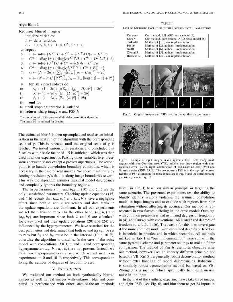
Algorithm 1

The estimated blur h is then upsampled and used as an initial-ization in the next run of the algorithm with the correspondingscale of g. This is repeated until the original scale of g isreached. We tested various configurations and concluded that5 scales with a scale factor of 1.5 is sufficient, which was thenused in all our experiments. Passing other variables (e.g. preci-sions) between scales except h proved superfluous. The secondpoint is to handle convolution boundary conditions, which isnecessary in the case of real images. We solve it naturally byforcing precisions γi ’s that lie along image boundaries to zero.This way the algorithm assumes maximal model discrepancyand completely ignores the boundary regions.

The hyperparameters a(·) and b(·) in (10) and (11) are theonly user-defined parameters. Checking update equations (15)and (16) reveals that (aα, bα) and (aν, bν) have a negligibleeffect since both α and ν are scalars and data terms inthe update equations are dominant. In all our experimentswe set them thus to zero. On the other hand, (aλ, bλ) and(aβ, bβ) are important since both λ and β are calculatedfor every pixel and their update equations (20) and (24) areinfluenced by the hyperparameters. We have searched for thebest parameters and determined that both aλ and aβ can be setto zero but bλ and bβ must be in the interval (10−9, 10−6),otherwise the algorithm is unstable. In the case of the noisemodel with conventional ARD, α and ν (and correspondinghyperparameters aα, bα, aν , bν) are not present. Instead, wehave new hyperparameters aγ , bγ , which we set in all ourexperiments to 0 and 10−4, respectively. This corresponds tofixing the number of degrees of freedom to zero.

V. EXPERIMENTS

We evaluated our method on both synthetically blurredimages as well as real images with unknown blur and com-pared its performance with other state-of-the-art methods

TABLE I

LIST OF METHODS INCLUDED IN THE EXPERIMENTAL EVALUATION

Fig. 6. Original images and PSFs used in our synthetic experiments.

Fig. 7. Sample of input images in our synthetic tests. Left: many smallregions with non-Gaussian error (7%), middle: one large region with non-Gaussian error (2.2%), right: combination of non-Gaussian error (5%) andGaussian noise (SNR=25dB). The ground-truth PSF is in the top-right corner.Results of PSF estimation for these inputs are in Fig. 9 and the correspondingprecision γi s is in Fig. 10.

(listed in Tab. I) based on similar principle or targeting thesame scenario. The presented experiments test the ability toblindly identify regions violating the assumed convolutionmodel in input images and to exclude such regions from blurestimation without affecting its accuracy. Our method is rep-resented in two flavors differing in the error model: Ours-αγwith common precision α and estimated degrees of freedom νin (4), and Ours-γ with conventional ARD and fixed degrees offreedom aγ and bγ in (6). The reason for this is to investigateif the more complex model with estimated degrees of freedomis beneficial in practice and in which scenarios. All methodsmarked in Tab. I as “our implementation” were run with thesame pyramid scheme and parameter settings to make a fairercomparison. The method of Pan16 resembles objective wiseour method, however uses an entirely different principle notbased on VB. Xu10 is a generally robust deconvolution methodwithout extra handling of model discrepancies. Babacan12is similarly robust deconvolution method but based on VB.Zhong13 is a method which specifically handles Gaussiannoise in the input.

In the first of the synthetic experiments we take three imagesand eight PSFs (see Fig. 6), and blur them to get 24 inputs in


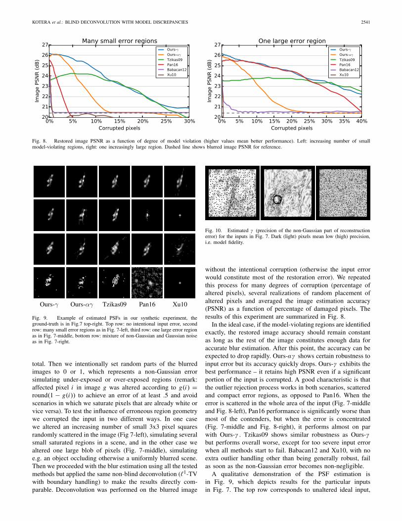
Fig. 8. Restored image PSNR as a function of degree of model violation (higher values mean better performance). Left: increasing number of smallmodel-violating regions, right: one increasingly large region. Dashed line shows blurred image PSNR for reference.

Fig. 9. Example of estimated PSFs in our synthetic experiment, theground-truth is in Fig.7 top-right. Top row: no intentional input error, secondrow: many small error regions as in Fig. 7-left, third row: one large error regionas in Fig. 7-middle, bottom row: mixture of non-Gaussian and Gaussian noiseas in Fig. 7-right.

total. Then we intentionally set random parts of the blurredimages to 0 or 1, which represents a non-Gaussian errorsimulating under-exposed or over-exposed regions (remark:affected pixel i in image g was altered according to g(i) =round(1 − g(i)) to achieve an error of at least .5 and avoidscenarios in which we saturate pixels that are already white orvice versa). To test the influence of erroneous region geometrywe corrupted the input in two different ways. In one casewe altered an increasing number of small 3x3 pixel squaresrandomly scattered in the image (Fig 7-left), simulating severalsmall saturated regions in a scene, and in the other case wealtered one large blob of pixels (Fig. 7-middle), simulatinge.g. an object occluding otherwise a uniformly blurred scene.Then we proceeded with the blur estimation using all the testedmethods but applied the same non-blind deconvolution (�1-TVwith boundary handling) to make the results directly com-parable. Deconvolution was performed on the blurred image

Fig. 10. Estimated γ (precision of the non-Gaussian part of reconstructionerror) for the inputs in Fig. 7. Dark (light) pixels mean low (high) precision,i.e. model fidelity.

without the intentional corruption (otherwise the input errorwould constitute most of the restoration error). We repeatedthis process for many degrees of corruption (percentage ofaltered pixels), several realizations of random placement ofaltered pixels and averaged the image estimation accuracy(PSNR) as a function of percentage of damaged pixels. Theresults of this experiment are summarized in Fig. 8.

In the ideal case, if the model-violating regions are identifiedexactly, the restored image accuracy should remain constantas long as the rest of the image constitutes enough data foraccurate blur estimation. After this point, the accuracy can beexpected to drop rapidly. Ours-αγ shows certain robustness toinput error but its accuracy quickly drops. Ours-γ exhibits thebest performance – it retains high PSNR even if a significantportion of the input is corrupted. A good characteristic is thatthe outlier rejection process works in both scenarios, scatteredand compact error regions, as opposed to Pan16. When theerror is scattered in the whole area of the input (Fig. 7-middleand Fig. 8-left), Pan16 performance is significantly worse thanmost of the contenders, but when the error is concentrated(Fig. 7-middle and Fig. 8-right), it performs almost on parwith Ours-γ . Tzikas09 shows similar robustness as Ours-γbut performs overall worse, except for too severe input errorwhen all methods start to fail. Babacan12 and Xu10, with noextra outlier handling other than being generally robust, failas soon as the non-Gaussian error becomes non-negligible.

A qualitative demonstration of the PSF estimation isin Fig. 9, which depicts results for the particular inputsin Fig. 7. The top row corresponds to unaltered ideal input,


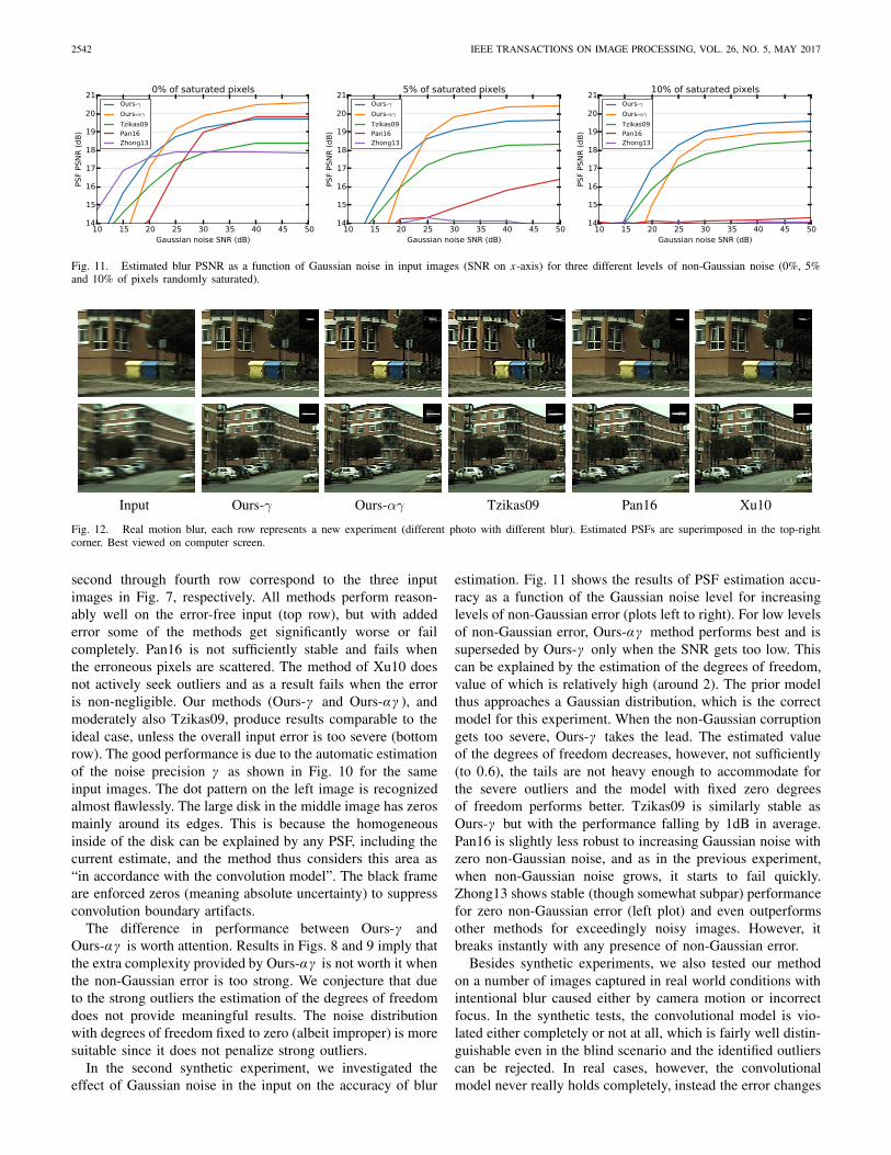
Fig. 11. Estimated blur PSNR as a function of Gaussian noise in input images (SNR on x-axis) for three different levels of non-Gaussian noise (0%, 5%and 10% of pixels randomly saturated).

Fig. 12. Real motion blur, each row represents a new experiment (different photo with different blur). Estimated PSFs are superimposed in the top-rightcorner. Best viewed on computer screen.

second through fourth row correspond to the three inputimages in Fig. 7, respectively. All methods perform reason-ably well on the error-free input (top row), but with addederror some of the methods get significantly worse or failcompletely. Pan16 is not sufficiently stable and fails whenthe erroneous pixels are scattered. The method of Xu10 doesnot actively seek outliers and as a result fails when the erroris non-negligible. Our methods (Ours-γ and Ours-αγ ), andmoderately also Tzikas09, produce results comparable to theideal case, unless the overall input error is too severe (bottomrow). The good performance is due to the automatic estimationof the noise precision γ as shown in Fig. 10 for the sameinput images. The dot pattern on the left image is recognizedalmost flawlessly. The large disk in the middle image has zerosmainly around its edges. This is because the homogeneousinside of the disk can be explained by any PSF, including thecurrent estimate, and the method thus considers this area as“in accordance with the convolution model”. The black frameare enforced zeros (meaning absolute uncertainty) to suppressconvolution boundary artifacts.

The difference in performance between Ours-γ andOurs-αγ is worth attention. Results in Figs. 8 and 9 imply thatthe extra complexity provided by Ours-αγ is not worth it whenthe non-Gaussian error is too strong. We conjecture that dueto the strong outliers the estimation of the degrees of freedomdoes not provide meaningful results. The noise distributionwith degrees of freedom fixed to zero (albeit improper) is moresuitable since it does not penalize strong outliers.

In the second synthetic experiment, we investigated theeffect of Gaussian noise in the input on the accuracy of blur

estimation. Fig. 11 shows the results of PSF estimation accu-racy as a function of the Gaussian noise level for increasinglevels of non-Gaussian error (plots left to right). For low levelsof non-Gaussian error, Ours-αγ method performs best and issuperseded by Ours-γ only when the SNR gets too low. Thiscan be explained by the estimation of the degrees of freedom,value of which is relatively high (around 2). The prior modelthus approaches a Gaussian distribution, which is the correctmodel for this experiment. When the non-Gaussian corruptiongets too severe, Ours-γ takes the lead. The estimated valueof the degrees of freedom decreases, however, not sufficiently(to 0.6), the tails are not heavy enough to accommodate forthe severe outliers and the model with fixed zero degreesof freedom performs better. Tzikas09 is similarly stable asOurs-γ but with the performance falling by 1dB in average.Pan16 is slightly less robust to increasing Gaussian noise withzero non-Gaussian noise, and as in the previous experiment,when non-Gaussian noise grows, it starts to fail quickly.Zhong13 shows stable (though somewhat subpar) performancefor zero non-Gaussian error (left plot) and even outperformsother methods for exceedingly noisy images. However, itbreaks instantly with any presence of non-Gaussian error.

Besides synthetic experiments, we also tested our methodon a number of images captured in real world conditions withintentional blur caused either by camera motion or incorrectfocus. In the synthetic tests, the convolutional model is vio-lated either completely or not at all, which is fairly well distin-guishable even in the blind scenario and the identified outlierscan be rejected. In real cases, however, the convolutionalmodel never really holds completely, instead the error changes


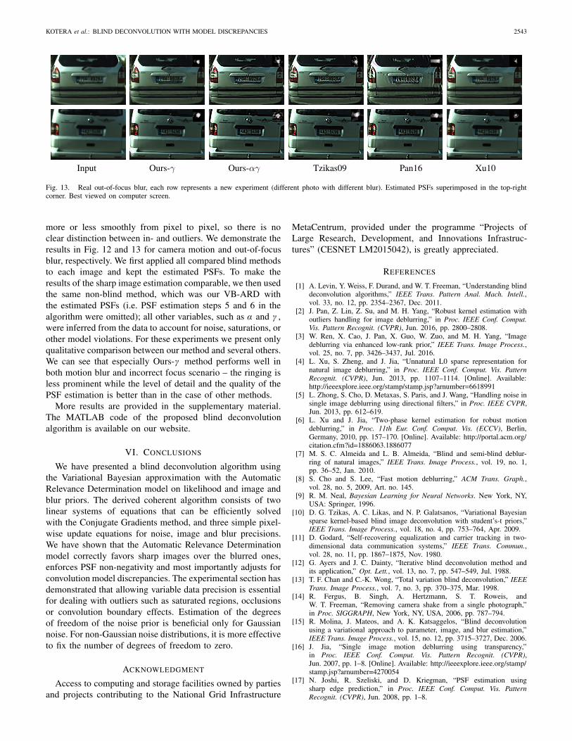
Fig. 13. Real out-of-focus blur, each row represents a new experiment (different photo with different blur). Estimated PSFs superimposed in the top-rightcorner. Best viewed on computer screen.

more or less smoothly from pixel to pixel, so there is noclear distinction between in- and outliers. We demonstrate theresults in Fig. 12 and 13 for camera motion and out-of-focusblur, respectively. We first applied all compared blind methodsto each image and kept the estimated PSFs. To make theresults of the sharp image estimation comparable, we then usedthe same non-blind method, which was our VB-ARD withthe estimated PSFs (i.e. PSF estimation steps 5 and 6 in thealgorithm were omitted); all other variables, such as α and γ ,were inferred from the data to account for noise, saturations, orother model violations. For these experiments we present onlyqualitative comparison between our method and several others.We can see that especially Ours-γ method performs well inboth motion blur and incorrect focus scenario – the ringing isless prominent while the level of detail and the quality of thePSF estimation is better than in the case of other methods.

More results are provided in the supplementary material.The MATLAB code of the proposed blind deconvolutionalgorithm is available on our website.

VI. CONCLUSIONS

We have presented a blind deconvolution algorithm usingthe Variational Bayesian approximation with the AutomaticRelevance Determination model on likelihood and image andblur priors. The derived coherent algorithm consists of twolinear systems of equations that can be efficiently solvedwith the Conjugate Gradients method, and three simple pixel-wise update equations for noise, image and blur precisions.We have shown that the Automatic Relevance Determinationmodel correctly favors sharp images over the blurred ones,enforces PSF non-negativity and most importantly adjusts forconvolution model discrepancies. The experimental section hasdemonstrated that allowing variable data precision is essentialfor dealing with outliers such as saturated regions, occlusionsor convolution boundary effects. Estimation of the degreesof freedom of the noise prior is beneficial only for Gaussiannoise. For non-Gaussian noise distributions, it is more effectiveto fix the number of degrees of freedom to zero.

ACKNOWLEDGMENT

Access to computing and storage facilities owned by partiesand projects contributing to the National Grid Infrastructure

MetaCentrum, provided under the programme “Projects ofLarge Research, Development, and Innovations Infrastruc-tures” (CESNET LM2015042), is greatly appreciated.

REFERENCES

[1] A. Levin, Y. Weiss, F. Durand, and W. T. Freeman, “Understanding blinddeconvolution algorithms,” IEEE Trans. Pattern Anal. Mach. Intell.,vol. 33, no. 12, pp. 2354–2367, Dec. 2011.

[2] J. Pan, Z. Lin, Z. Su, and M. H. Yang, “Robust kernel estimation withoutliers handling for image deblurring,” in Proc. IEEE Conf. Comput.Vis. Pattern Recognit. (CVPR), Jun. 2016, pp. 2800–2808.

[3] W. Ren, X. Cao, J. Pan, X. Guo, W. Zuo, and M. H. Yang, “Imagedeblurring via enhanced low-rank prior,” IEEE Trans. Image Process.,vol. 25, no. 7, pp. 3426–3437, Jul. 2016.

[4] L. Xu, S. Zheng, and J. Jia, “Unnatural L0 sparse representation fornatural image deblurring,” in Proc. IEEE Conf. Comput. Vis. PatternRecognit. (CVPR), Jun. 2013, pp. 1107–1114. [Online]. Available:http://ieeexplore.ieee.org/stamp/stamp.jsp?arnumber=6618991

[5] L. Zhong, S. Cho, D. Metaxas, S. Paris, and J. Wang, “Handling noise insingle image deblurring using directional filters,” in Proc. IEEE CVPR,Jun. 2013, pp. 612–619.

[6] L. Xu and J. Jia, “Two-phase kernel estimation for robust motiondeblurring,” in Proc. 11th Eur. Conf. Comput. Vis. (ECCV), Berlin,Germany, 2010, pp. 157–170. [Online]. Available: http://portal.acm.org/citation.cfm?id=1886063.1886077

[7] M. S. C. Almeida and L. B. Almeida, “Blind and semi-blind deblur-ring of natural images,” IEEE Trans. Image Process., vol. 19, no. 1,pp. 36–52, Jan. 2010.

[8] S. Cho and S. Lee, “Fast motion deblurring,” ACM Trans. Graph.,vol. 28, no. 5, 2009, Art. no. 145.

[9] R. M. Neal, Bayesian Learning for Neural Networks. New York, NY,USA: Springer, 1996.

[10] D. G. Tzikas, A. C. Likas, and N. P. Galatsanos, “Variational Bayesiansparse kernel-based blind image deconvolution with student’s-t priors,”IEEE Trans. Image Process., vol. 18, no. 4, pp. 753–764, Apr. 2009.

[11] D. Godard, “Self-recovering equalization and carrier tracking in two-dimensional data communication systems,” IEEE Trans. Commun.,vol. 28, no. 11, pp. 1867–1875, Nov. 1980.

[12] G. Ayers and J. C. Dainty, “Iterative blind deconvolution method andits application,” Opt. Lett., vol. 13, no. 7, pp. 547–549, Jul. 1988.

[13] T. F. Chan and C.-K. Wong, “Total variation blind deconvolution,” IEEETrans. Image Process., vol. 7, no. 3, pp. 370–375, Mar. 1998.

[14] R. Fergus, B. Singh, A. Hertzmann, S. T. Roweis, andW. T. Freeman, “Removing camera shake from a single photograph,”in Proc. SIGGRAPH, New York, NY, USA, 2006, pp. 787–794.

[15] R. Molina, J. Mateos, and A. K. Katsaggelos, “Blind deconvolutionusing a variational approach to parameter, image, and blur estimation,”IEEE Trans. Image Process., vol. 15, no. 12, pp. 3715–3727, Dec. 2006.

[16] J. Jia, “Single image motion deblurring using transparency,”in Proc. IEEE Conf. Comput. Vis. Pattern Recognit. (CVPR),Jun. 2007, pp. 1–8. [Online]. Available: http://ieeexplore.ieee.org/stamp/stamp.jsp?arnumber=4270054

[17] N. Joshi, R. Szeliski, and D. Kriegman, “PSF estimation usingsharp edge prediction,” in Proc. IEEE Conf. Comput. Vis. PatternRecognit. (CVPR), Jun. 2008, pp. 1–8.


[18] Q. Shan, J. Jia, and A. Agarwala, “High-quality motion deblur-ring from a single image,” in Proc. SIGGRAPH ACM SIGGRAPH ,New York, NY, USA, 2008, pp. 1–10.

[19] D. Perrone and P. Favaro, “A clearer picture of total variation blinddeconvolution,” IEEE Trans. Pattern Anal. Mach. Intell, vol. 38, no. 6,pp. 1041–1055, Jun. 2016.

[20] J. Miskin and D. J. MacKay, “Ensemble learning for blind imageseparation and deconvolution,” in Advances in Independent Compo-nent Analysis, M. Girolami, Ed. London, U.K.: Springer-Verlag, 2000,pp. 123–142.

[21] N. P. Galatsanos, V. Z. Mesarovic, R. Molina, and A. K. Katsaggelos,“Hierarchical Bayesian image restoration from partially-known blurs,”IEEE Trans. Image Process., vol. 9, no. 10, pp. 1784–1797, Oct. 2000.

[22] S. D. Babacan, R. Molina, M. N. Do, and A. K. Katsaggelos, “Bayesianblind deconvolution with general sparse image priors,” in ComputerVision—ECCV. Berlin, Germany: Springer, 2012, pp. 341–355.

[23] F. Sroubek, V. Smídl, and J. Kotera, “Understanding image priors inblind deconvolution,” in Proc. IEEE Int. Conf. Image Process., 2014,pp. 4492–4496.

[24] J. A. Palmer, K. Kreutz-Delgado, and S. Makeig, “Strong sub- and super-gaussianity,” Latent Variable Anal. Signal Separat., vol. 6365, pp. 303–310, Jan. 2010.

[25] D. Wipf and H. Zhang, “Revisiting Bayesian blind decon-volution,” J. Mach. Learn. Res., vol. 15, pp. 3775–3814, Nov. 2014. [Online]. Available: http://research.microsoft.com/apps/pubs/ default.aspx?id=192590

[26] P. Ruiz, X. Zhou, J. Mateos, R. Molina, and A. K. Katsaggelos,“Variational Bayesian blind image deconvolution: A review,” Digit.Signal Process., vol. 47, pp. 116–127, Dec. 2015. [Online]. Available:http://dx.doi.org/10.1016/j.dsp.2015.04.012

[27] D. F. Andrews and C. L. Mallows, “Scale mixtures of normaldistributions,” J. Roy. Statist. Soc. B, Methodol., vol. 36, no. 1,pp. 99–102, 1974. [Online]. Available: http://www.jstor.org/stable/2984774

[28] G. Chantas, N. Galatsanos, A. Likas, and M. Saunders, “VariationalBayesian image restoration based on a product of t-distributions imageprior,” IEEE Trans. Image Process., vol. 17, no. 10, pp. 1795–1805,Oct. 2008.

[29] G. Chantas, N. P. Galatsanos, R. Molina, and A. K. Katsaggelos,“Variational Bayesian image restoration with a product of spatiallyweighted total variation image priors,” IEEE Trans. Image Process.,vol. 19, no. 2, pp. 351–362, Feb. 2010.

[30] H. Zhang, D. Wipf, and Y. Zhang, “Multi-observation blind deconvo-lution with an adaptive sparse prior,” IEEE Trans. Pattern Anal. Mach.Intell., vol. 36, no. 8, pp. 1628–1643, Aug. 2014.

[31] W. Dong, H. Feng, Z. Xu, and Q. Li, “Blind image deconvolu-tion using the fields of experts prior,” Opt. Commun., vol. 285,no. 24, pp. 5051–5061, 2012.

[32] J. Christmas and R. Everson, “Robust autoregression: Student-t inno-vations using variational Bayes,” IEEE Trans. Signal Process., vol. 59,no. 1, pp. 48–57, Jan. 2011.

[33] T. Kohler, X. Huang, F. Schebesch, A. Aichert, A. Maier, andJ. Hornegger, “Robust multiframe super-resolution employing iterativelyre-weighted minimization,” IEEE Trans. Comput. Imag., vol. 2, no. 1,pp. 42–58, Mar. 2016.

[34] A. Matakos, S. Ramani, and J. A. Fessler, “Accelerated edge-preservingimage restoration without boundary artifacts,” IEEE Trans. ImageProcess., vol. 22, no. 5, pp. 2019–2029, May 2013.

[35] M. S. C. Almeida and M. A. T. Figueiredo, “Deconvolving imageswith unknown boundaries using the alternating direction method ofmultipliers,” IEEE Trans. Image Process., vol. 22, no. 8, pp. 3074–3086,Aug. 2013.

[36] S. Cho, J. Wang, and S. Lee, “Handling outliers in non-blindimage deconvolution,” in Proc. Int. Conf. Comput. Vis., Nov. 2011,pp. 495–502.

[37] R. Tezaur, T. Kamata, L. Hong, and S. S. Slonaker, “A systemfor estimating optics blur psfs from test chart images,” Proc. SPIE,vol. 9404, pp. 94040D-1–94040D-10, Feb. 2015. [Online]. Available:http://dx.doi.org/10.1117/12.2081458

[38] C. M. Bishop, Pattern Recognition and Machine Learning. New york,NY, USA: Springer-Verlag, 2006.

[39] D. Krishnan, T. Tay, and R. Fergus, “Blind deconvolution using anormalized sparsity measure,” in Proc. CVPR, 2011, pp. 233–240.

[40] S. Boyd, N. Parikh, E. Chu, B. Peleato, and J. Eckstein, “Distributedoptimization and statistical learning via the alternating direction methodof multipliers,” Found. Trends Mach. Learn., vol. 3, no. 1, pp. 1–122,Jan. 2011.

Jan Kotera received the master’s and Ph.D. degreesin mathematical modeling and computer sciencefrom Charles University in Prague, Czech Republic,in 2011 and 2014, respectively, where he is currentlypursuing the Ph.D. degree in computer science.Since 2011, he has been with the Institute of Infor-mation Theory and Automation, Czech Academyof Sciences. He has authored several conferencepapers on blind deconvolution and related topics.His current research interests include all aspectsof digital image processing and pattern recognition,

particularly blind deconvolution and image restoration in general.

Václav Šmídl (M’05) received the Ph.D. degreein electrical engineering from the Trinity CollegeDublin, Ireland, in 2004. Since 2004, he has beena Researcher with the Institute of Information The-ory and Automation, Czech Academy of Sciences,Prague, Czech Republic. He authored one Springermonograph Variational Bayes method in SignalProcessing. His research interests are advancedBayesian methods for signal and image processing.

Filip Šroubek (M’08) received the M.S. degree incomputer science from Czech Technical University,Prague, Czech Republic, in 1998, and the Ph.D.degree in computer science from Charles University,Prague, Czech Republic, in 2003. From 2004 to2006, he was on a post-doctoral position with theInstituto de Optica, CSIC, Madrid, Spain. In 2010and 2011, he was the Fulbright Visiting Scholar withthe University of California at Santa Cruz, SantaCruz. He is currently with the Institute of Infor-mation Theory and Automation, Czech Academy of

Sciences, and teaches at Charles University. He has authored eight bookchapters and over 70 journal and conference papers on image fusion, blinddeconvolution, superresolution, and related topics.

Documents

IEEE TRANSACTIONS ON IMAGE PROCESSING, VOL. …library.utia.cas.cz/separaty/2017/ZOI/kotera-0474858.pdf · Blind Deconvolution With Model Discrepancies Jan Kotera, Student Member,