IEEE TRANSACTIONS ON IMAGE PROCESSING 1 Tasking on …live.ece.utexas.edu/research/IR/LWIR_TIP.pdf · IEEE TRANSACTIONS ON IMAGE PROCESSING 1 Tasking on Natural Statistics of Infrared

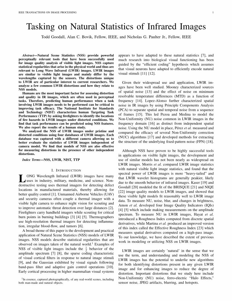
IEEE TRANSACTIONS ON IMAGE PROCESSING 1

Tasking on Natural Statistics of Infrared ImagesTodd Goodall, Alan C. Bovik, Fellow, IEEE, and Nicholas G. Paulter Jr., Fellow, IEEE

Abstract—Natural Scene Statistics (NSS) provide powerfulperceptually relevant tools that have been successfully usedfor image quality analysis of visible light images. NSS capturestatistical regularities that arise in the physical world and thus arerelevant to Long Wave Infrared (LWIR) images. LWIR imagesare similar to visible light images and mainly differ by thewavelengths captured by the sensors. The distortions uniqueto LWIR are of particular interest to current researchers. Weanalyze a few common LWIR distortions and how they relate toNSS models.

Humans are the most important factor for assessing distortionand quality in IR images, which are often used in perceptualtasks. Therefore, predicting human performance when a taskinvolving LWIR images needs to be performed can be critical toimproving task efficacy. The National Institute for Standardsand Technology (NIST) characterizes human Targeting TaskPerformance (TTP) by asking firefighters to identify the locationsof fire hazards in LWIR images under distorted conditions. Wefind that task performance can be predicted using NSS features.We also report the results of a human study.

We analyzed the NSS of LWIR images under pristine anddistorted conditions using four databases of LWIR images. Eachdatabase was captured with a different camera allowing us tobetter evaluate the statistics of LWIR images independent ofcamera model. We find that models of NSS are also effectivefor measuring distortions in the presence of other independentdistortions.

Index Terms—NSS, LWIR, NIST, TTP

I. INTRODUCTION

LONG Wavelength Infrared (LWIR) images have manyuses in industry, military, medicine, and science. Non-

destructive testing uses thermal imagers for detecting defectlocations in manufactured materials, thereby allowing forbetter quality control [1]. Unmanned Airborne Vehicles (UAV)and security cameras often couple a thermal imager with avisible light camera to enhance night vision for scouting andto improve automatic threat detection over large distances [2].Firefighters carry handheld imagers while scouting for criticalburn points in burning buildings [3] [4] [5]. Thermographersuse high-resolution thermal imagers for detecting inflamma-tion, irregular blood-flow, and tumors [6].

A broad theme of this paper is the development and practicalapplication of Natural Scene Statistics (NSS) models of LWIRimages. NSS models describe statistical regularities that areobserved on images taken of the natural world.1 Examples ofNSS of visible light images include the 1

f behavior of theamplitude spectrum [7] [8], the sparse coding characteristicof visual cortical filters in response to natural image stimuli[9], and the Gaussian exhibited by visual signals followingband-pass filter and adaptive gain control operations [10].Early cortical processing in higher mammalian visual systems

1In essence, captured photographically, of any real-world scenes, includingboth man-made and natural objects.

appears to have adapted to these natural statistics [7], andmuch research into biological visual functioning has beenguided by the “efficient coding” hypothesis which assumesthat visual neurons have adapted to efficiently encode naturalvisual stimuli [11] [12].

Given their widespread use and application, LWIR im-ages have been well studied. Mooney characterized sourcesof spatial noise [13] and the effect of noise on minimumresolvable temperature differences (MTD) as a function offrequency [14]. Lopez-Alonso further characterized spatialnoise in IR images by using Principle Components Analysis(PCA) to separate spatial and temporal noise from a sequenceof frames [15]. This led Pezoa and Medina to model theNon-Uniformity (NU) noise common in LWIR images in thefrequency domain [16] as distinct from independent spatialnoise. Using the NU model in place, Perez et al. measured andcompared the efficacy of several Non-Uniformity correction(NUC) algorithms [17] and developed methods for extractingthe structure of the underlying fixed-pattern noise (FPN) [18].

Although NSS have proven to be highly successful toolsin applications on visible light images, the development anduse of similar models has not been nearly as widespread onLWIR images. Morris et al. compared LWIR image statisticswith natural visible light image statistics, and found that thespectral power of LWIR images is more “heavy-tailed” andthat LWIR wavelet histograms are generally peakier, likelydue to the smooth behavior of infrared images. Kaser [19] andGoodall [20] modeled the fit of the BRISQUE [21] and NIQE[22] image quality models to LWIR images, and showed thatthese visible light models fit reasonably well to LWIR imagedata. To measure NU, noise, blur, and changes in brightness,Amon et al. developed four Image Quality Indicators (IQIs)[4] [5] which include making measurements on the amplitudespectrum. To measure NU in LWIR images, Hayat et al.introduced a Roughness Index computed from discrete spatialderivatives, while Martina et al. produced an improved versionof this index called the Effective Roughness Index [23] whichmeasures spatial derivatives computed on a high-pass image.To our knowledge, we have described the extent of previouswork in modeling or utilizing NSS on LWIR images.

LWIR images are certainly ’natural’ in the sense that weuse the term, and understanding and modeling the NSS ofLWIR images has the potential to underlie new algorithmsfor both identifying distortions present in any given LWIRimage and for enhancing images to reduce the degree ofdistortion. Important distortions that we study here includeNon-Uniformity (NU) noise, ferro-electric “Halo Effects,”sensor noise, JPEG artifacts, blurring, and hotspots.


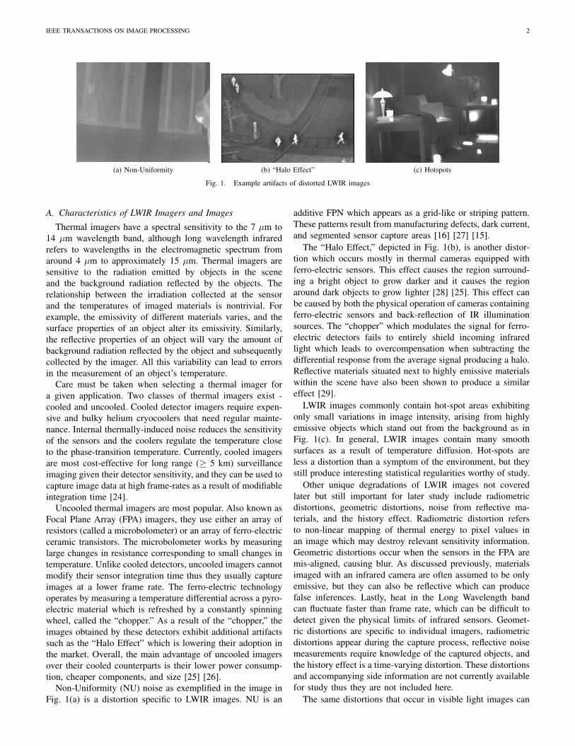
(a) Non-Uniformity (b) “Halo Effect” (c) Hotspots

Fig. 1. Example artifacts of distorted LWIR images

A. Characteristics of LWIR Imagers and Images

Thermal imagers have a spectral sensitivity to the 7 µm to14 µm wavelength band, although long wavelength infraredrefers to wavelengths in the electromagnetic spectrum fromaround 4 µm to approximately 15 µm. Thermal imagers aresensitive to the radiation emitted by objects in the sceneand the background radiation reflected by the objects. Therelationship between the irradiation collected at the sensorand the temperatures of imaged materials is nontrivial. Forexample, the emissivity of different materials varies, and thesurface properties of an object alter its emissivity. Similarly,the reflective properties of an object will vary the amount ofbackground radiation reflected by the object and subsequentlycollected by the imager. All this variability can lead to errorsin the measurement of an object’s temperature.

Care must be taken when selecting a thermal imager fora given application. Two classes of thermal imagers exist -cooled and uncooled. Cooled detector imagers require expen-sive and bulky helium cryocoolers that need regular mainte-nance. Internal thermally-induced noise reduces the sensitivityof the sensors and the coolers regulate the temperature closeto the phase-transition temperature. Currently, cooled imagersare most cost-effective for long range (≥ 5 km) surveillanceimaging given their detector sensitivity, and they can be used tocapture image data at high frame-rates as a result of modifiableintegration time [24].

Uncooled thermal imagers are most popular. Also known asFocal Plane Array (FPA) imagers, they use either an array ofresistors (called a microbolometer) or an array of ferro-electricceramic transistors. The microbolometer works by measuringlarge changes in resistance corresponding to small changes intemperature. Unlike cooled detectors, uncooled imagers cannotmodify their sensor integration time thus they usually captureimages at a lower frame rate. The ferro-electric technologyoperates by measuring a temperature differential across a pyro-electric material which is refreshed by a constantly spinningwheel, called the “chopper.” As a result of the “chopper,” theimages obtained by these detectors exhibit additional artifactssuch as the “Halo Effect” which is lowering their adoption inthe market. Overall, the main advantage of uncooled imagersover their cooled counterparts is their lower power consump-tion, cheaper components, and size [25] [26].

Non-Uniformity (NU) noise as exemplified in the image inFig. 1(a) is a distortion specific to LWIR images. NU is an

additive FPN which appears as a grid-like or striping pattern.These patterns result from manufacturing defects, dark current,and segmented sensor capture areas [16] [27] [15].

The “Halo Effect,” depicted in Fig. 1(b), is another distor-tion which occurs mostly in thermal cameras equipped withferro-electric sensors. This effect causes the region surround-ing a bright object to grow darker and it causes the regionaround dark objects to grow lighter [28] [25]. This effect canbe caused by both the physical operation of cameras containingferro-electric sensors and back-reflection of IR illuminationsources. The “chopper” which modulates the signal for ferro-electric detectors fails to entirely shield incoming infraredlight which leads to overcompensation when subtracting thedifferential response from the average signal producing a halo.Reflective materials situated next to highly emissive materialswithin the scene have also been shown to produce a similareffect [29].

LWIR images commonly contain hot-spot areas exhibitingonly small variations in image intensity, arising from highlyemissive objects which stand out from the background as inFig. 1(c). In general, LWIR images contain many smoothsurfaces as a result of temperature diffusion. Hot-spots areless a distortion than a symptom of the environment, but theystill produce interesting statistical regularities worthy of study.

Other unique degradations of LWIR images not coveredlater but still important for later study include radiometricdistortions, geometric distortions, noise from reflective ma-terials, and the history effect. Radiometric distortion refersto non-linear mapping of thermal energy to pixel values inan image which may destroy relevant sensitivity information.Geometric distortions occur when the sensors in the FPA aremis-aligned, causing blur. As discussed previously, materialsimaged with an infrared camera are often assumed to be onlyemissive, but they can also be reflective which can producefalse inferences. Lastly, heat in the Long Wavelength bandcan fluctuate faster than frame rate, which can be difficult todetect given the physical limits of infrared sensors. Geomet-ric distortions are specific to individual imagers, radiometricdistortions appear during the capture process, reflective noisemeasurements require knowledge of the captured objects, andthe history effect is a time-varying distortion. These distortionsand accompanying side information are not currently availablefor study thus they are not included here.

The same distortions that occur in visible light images can


(a) NIST (b) KASER

(c) MORRIS (d) OSU

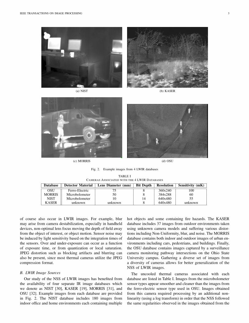
Fig. 2. Example images from 4 LWIR databases

TABLE ICAMERAS ASSOCIATED WITH THE 4 LWIR DATABASES

Database Detector Material Lens Diameter (mm) Bit Depth Resolution Sensitivity (mK)OSU Ferro-Electric 75 8 360x240 100

MORRIS Microbolometer 50 8 384x288 60NIST Microbolometer 10 14 640x480 55

KASER unknown unknown 8 640x480 unknown

of course also occur in LWIR images. For example, blurmay arise from camera destabilization, especially in handhelddevices, non-optimal lens focus moving the depth of field awayfrom the object of interest, or object motion. Sensor noise maybe induced by light sensitivity based on the integration times ofthe sensors. Over and under-exposure can occur as a functionof exposure time, or from quantization or local saturation.JPEG distortion such as blocking artifacts and blurring canalso be present, since most thermal cameras utilize the JPEGcompression format.

B. LWIR Image Sources

Our study of the NSS of LWIR images has benefited fromthe availability of four separate IR image databases whichwe denote as NIST [30], KASER [19], MORRIS [31], andOSU [32]. Example images from each database are providedin Fig. 2. The NIST database includes 180 images fromindoor office and home environments each containing multiple

hot objects and some containing fire hazards. The KASERdatabase includes 37 images from outdoor environments takenusing unknown camera models and suffering various distor-tions including Non-Uniformity, blur, and noise. The MORRISdatabase contains both indoor and outdoor images of urban en-vironments including cars, pedestrians, and buildings. Finally,the OSU database contains images captured by a surveillancecamera monitoring pathway intersections on the Ohio StateUniversity campus. Gathering a diverse set of images froma diversity of cameras allows for better generalization of theNSS of LWIR images.

The uncooled thermal cameras associated with eachdatabase are listed in Table I. Images from the microbolometersensor types appear smoother and cleaner than the images fromthe ferro-electric sensor type used in OSU. Images obtainedfrom this camera required processing by an additional non-linearity (using a log transform) in order that the NSS followedthe same regularities observed in the images obtained from the


Pristine Distortion Level 1 Distortion Level 2 Distortion Level 3

I

−1.0 −0.5 0.0 0.5 1.0MSCN coefficients

0.0

0.5

1.0Number of co

efficients (norm

alized)

org (scale 1)

org (scale 2)

org (scale 3)

−1.0 −0.5 0.0 0.5 1.0MSCN coefficients

0.0

0.5

1.0

Num

be of co

effic

ients

(no m

aliz

ed)

o g

NU

AWN

blu

JPEG

hotspot

halo

−1.0 −0.5 0.0 0.5 1.0MSCN coefficien s

0.0

0.5

1.0

Num

ber of co

effic

ien s

(norm

aliz

ed)

org

NU

AWN

blur

JPEG

−1.0 −0.5 0.0 0.5 1.0MSCN coefficien s

0.0

0.5

1.0

Num

ber of co

effic

ien s

(norm

aliz

ed)

org

NU

AWN

blur

JPEG

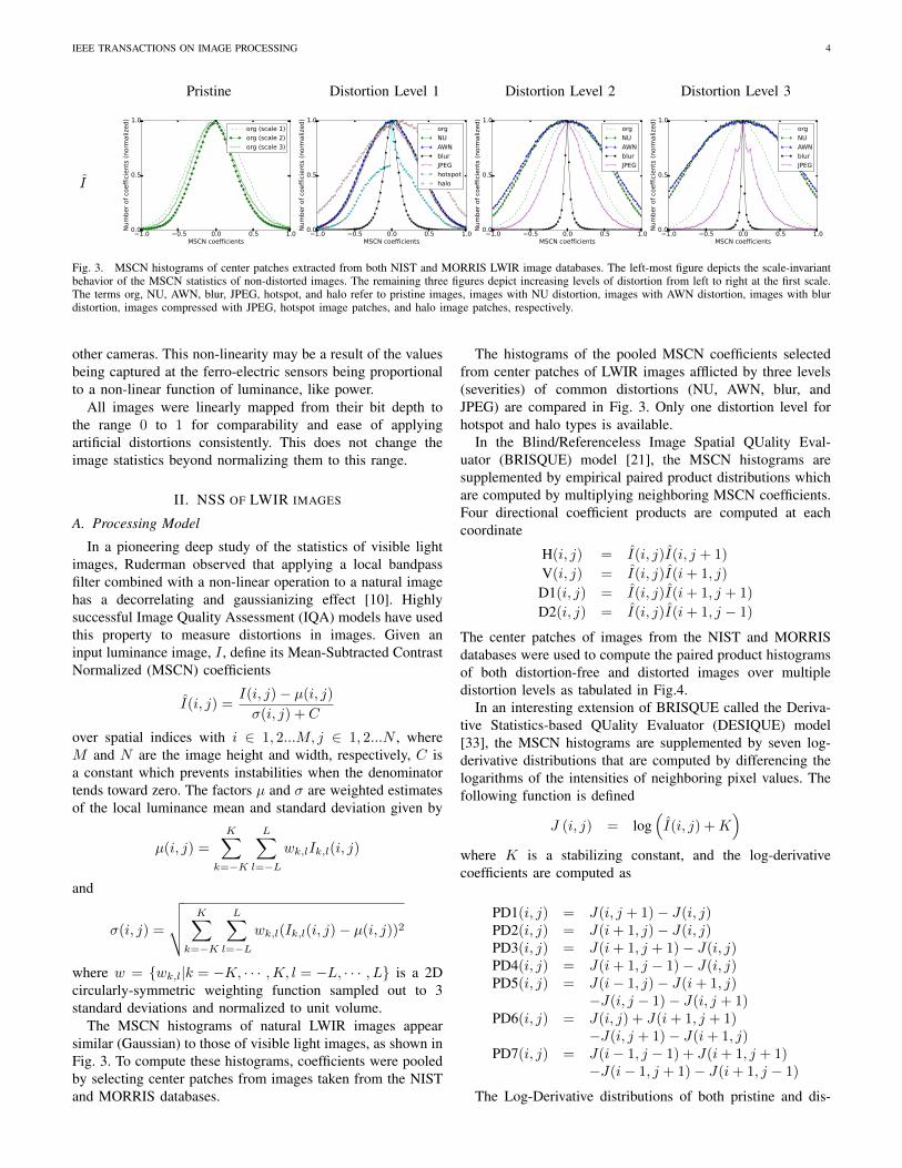
Fig. 3. MSCN histograms of center patches extracted from both NIST and MORRIS LWIR image databases. The left-most figure depicts the scale-invariantbehavior of the MSCN statistics of non-distorted images. The remaining three figures depict increasing levels of distortion from left to right at the first scale.The terms org, NU, AWN, blur, JPEG, hotspot, and halo refer to pristine images, images with NU distortion, images with AWN distortion, images with blurdistortion, images compressed with JPEG, hotspot image patches, and halo image patches, respectively.

other cameras. This non-linearity may be a result of the valuesbeing captured at the ferro-electric sensors being proportionalto a non-linear function of luminance, like power.

All images were linearly mapped from their bit depth tothe range 0 to 1 for comparability and ease of applyingartificial distortions consistently. This does not change theimage statistics beyond normalizing them to this range.

II. NSS OF LWIR IMAGES

A. Processing Model

In a pioneering deep study of the statistics of visible lightimages, Ruderman observed that applying a local bandpassfilter combined with a non-linear operation to a natural imagehas a decorrelating and gaussianizing effect [10]. Highlysuccessful Image Quality Assessment (IQA) models have usedthis property to measure distortions in images. Given aninput luminance image, I , define its Mean-Subtracted ContrastNormalized (MSCN) coefficients

I(i, j) =I(i, j)− µ(i, j)

σ(i, j) + C

over spatial indices with i ∈ 1, 2...M, j ∈ 1, 2...N , whereM and N are the image height and width, respectively, C isa constant which prevents instabilities when the denominatortends toward zero. The factors µ and σ are weighted estimatesof the local luminance mean and standard deviation given by

µ(i, j) =

K∑k=−K

L∑l=−L

wk,lIk,l(i, j)

and

σ(i, j) =

√√√√ K∑k=−K

L∑l=−L

wk,l(Ik,l(i, j)− µ(i, j))2

where w = {wk,l|k = −K, · · · ,K, l = −L, · · · , L} is a 2Dcircularly-symmetric weighting function sampled out to 3standard deviations and normalized to unit volume.

The MSCN histograms of natural LWIR images appearsimilar (Gaussian) to those of visible light images, as shown inFig. 3. To compute these histograms, coefficients were pooledby selecting center patches from images taken from the NISTand MORRIS databases.

The histograms of the pooled MSCN coefficients selectedfrom center patches of LWIR images afflicted by three levels(severities) of common distortions (NU, AWN, blur, andJPEG) are compared in Fig. 3. Only one distortion level forhotspot and halo types is available.

In the Blind/Referenceless Image Spatial QUality Eval-uator (BRISQUE) model [21], the MSCN histograms aresupplemented by empirical paired product distributions whichare computed by multiplying neighboring MSCN coefficients.Four directional coefficient products are computed at eachcoordinate

H(i, j) = I(i, j)I(i, j + 1)

V(i, j) = I(i, j)I(i+ 1, j)

D1(i, j) = I(i, j)I(i+ 1, j + 1)

D2(i, j) = I(i, j)I(i+ 1, j − 1)

The center patches of images from the NIST and MORRISdatabases were used to compute the paired product histogramsof both distortion-free and distorted images over multipledistortion levels as tabulated in Fig.4.

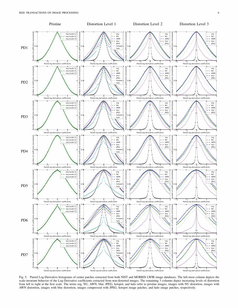
In an interesting extension of BRISQUE called the Deriva-tive Statistics-based QUality Evaluator (DESIQUE) model[33], the MSCN histograms are supplemented by seven log-derivative distributions that are computed by differencing thelogarithms of the intensities of neighboring pixel values. Thefollowing function is defined

J (i, j) = log(I(i, j) +K

)where K is a stabilizing constant, and the log-derivativecoefficients are computed as

PD1(i, j) = J(i, j + 1)− J(i, j)PD2(i, j) = J(i+ 1, j)− J(i, j)PD3(i, j) = J(i+ 1, j + 1)− J(i, j)PD4(i, j) = J(i+ 1, j − 1)− J(i, j)PD5(i, j) = J(i− 1, j)− J(i+ 1, j)

−J(i, j − 1)− J(i, j + 1)PD6(i, j) = J(i, j) + J(i+ 1, j + 1)

−J(i, j + 1)− J(i+ 1, j)PD7(i, j) = J(i− 1, j − 1) + J(i+ 1, j + 1)

−J(i− 1, j + 1)− J(i+ 1, j − 1)

The Log-Derivative distributions of both pristine and dis-



H

−0.10 −0.05 0.00 0.05 0.10Paired product coefficients

0.0

0.5

1.0Number of co

efficients (norm

alized)

org (scale 1)

org (scale 2)

org (scale 3)

−0.10 −0.05 0.00 0.05 0.10Paired prod ct coefficients

0.0

0.5

1.0

N mber of coefficients (norm

alized)

org

NU

AWN

bl r

JPEG

hotspot

halo


0.0

0.5

1.0

Number of co

efficients (norm

ali

ed)

org

NU

AWN

blur

JPEG


0.0

0.5

1.0

Number of co

efficients (norm

ali

ed)

org

NU

AWN

blur

JPEG

V


0.0

0.5

1.0

Number of co

efficients (norm

alized)

org (scale 1)

org (scale 2)

org (scale 3)


0.0

0.5

1.0


alized)

org

NU

AWN

bl r

JPEG

hotspot

halo


0.0

0.5

1.0

Number of co

efficients (norm

ali

ed)

org

NU

AWN

blur

JPEG


0.0

0.5

1.0

Number of co

efficients (norm

ali

ed)

org

NU

AWN

blur

JPEG

D1


0.0

0.5

1.0

Number of co

efficients (norm

alized)

org (scale 1)

org (scale 2)

org (scale 3)


0.0

0.5

1.0


alized)

org

NU

AWN

bl r

JPEG

hotspot

halo


0.0

0.5

1.0

Number of co

efficients (norm

ali

ed)

org

NU

AWN

blur

JPEG


0.0

0.5

1.0

Number of co

efficients (norm

ali

ed)

org

NU

AWN

blur

JPEG

D2


0.0

0.5

1.0

Number of co

efficients (norm

alized)

org (scale 1)

org (scale 2)

org (scale 3)


0.0

0.5

1.0


alized)

org

NU

AWN

bl r

JPEG

hotspot

halo


0.0

0.5

1.0

Number of co

efficients (norm

ali

ed)

org

NU

AWN

blur

JPEG


0.0

0.5

1.0

Number of co

efficients (norm

ali

ed)

org

NU

AWN

blur

JPEG

Fig. 4. Paired product histograms of center patches extracted from both NIST and MORRIS LWIR image databases. The left-most column depicts thescale-invariant behavior of paired products extracted from non-distorted images. The remaining 3 columns depict increasing levels of distortion from leftto right at the first scale. The terms org, NU, AWN, blur, JPEG, hotspot, and halo refer to pristine images, images with NU distortion, images with AWNdistortion, images with blur distortion, images compressed with JPEG, hotspot image patches, and halo image patches, respectively.

torted images over multiple distortion levels are plotted in Fig.5.

Perceptual neurons in the early stages of the human visualsystem form responses that capture information over multipleorientations and scales. These responses have been success-fully approximated by steerable filters, with the steerablepyramid decomposition being most popular [34] [35] [36].

The Distortion Identification-based Image Verity and IN-tegrity Evaluation (DIIVINE) [36] index predicts image qual-ity using coefficients generated from the steerable pyramidovercomplete wavelet decomposition. Oriented image sub-bands are divisively normalized by dividing the local contrastestimated from neighboring subbands and scales.

The divisively normalized steerable pyramid orientationsubbands for center patches extracted from one scale and sixorientations for both distortion-free and distorted images areplotted in Fig. 6. Each band is denoted dθα where α denotesthe level and θ ∈ {0◦, 30◦, 60◦, 90◦, 120◦, 150◦}.

B. Distortion Models

We next describe the generative noise models used to createdistorted LWIR images. Pezoa and Medina developed a modelof Non-Uniformity which can be used to artificially distortpristine images [16]. Based on a spectral analysis of NU, theyproposed the model

|I(u, v)| = Buexp

(− (u− u0)

2

2σ2u

)

+ Bvexp

(− (v − v0)

2

2σ2v

)

6 I(u, v) ∼ U[−π, π]

where I is the Fourier Transform representation of the noiseimage, Bu = Bv = 5.2, σu = σv = 2.5, and where U[a, b]denotes the uniform distribution on [a, b]. The severity ofNU can be controlled by scaling the dynamic range usinga standard deviation parameter σNU. Levels 1-3 of distortionwere generated by setting σNU = {0.0025, 0.01375, 0.025}.



PD1

−2 −1 0 1 2Paired log-derivative coefficients

0.0

0.5

1.0Number of co

efficients (norm

alized)

org (scale 1)

org (scale 2)

org (scale 3)

−2 −1 0 1 2Paired log-derivative coefficient

0.0

0.5

1.0

Number of co

efficient (norm

aliz

ed)

org

NU

AWN

blur

JPEG

hot pot

halo


0.0

0.5

1.0


alized)

org

NU

AWN

bl r

JPEG


0.0

0.5

1.0


alized)

org

NU

AWN

bl r

JPEG

PD2


0.0

0.5

1.0

Number of co

efficients (norm

alized)

org (scale 1)

org (scale 2)

org (scale 3)


0.0

0.5

1.0

Number of co

efficient (norm

aliz

ed)

org

NU

AWN

blur

JPEG

hot pot

halo


0.0

0.5

1.0


alized)

org

NU

AWN

bl r

JPEG


0.0

0.5

1.0


alized)

org

NU

AWN

bl r

JPEG

PD3


0.0

0.5

1.0

Number of co

efficients (norm

alized)

org (scale 1)

org (scale 2)

org (scale 3)


0.0

0.5

1.0

Number of co

efficient (norm

aliz

ed)

org

NU

AWN

blur

JPEG

hot pot

halo


0.0

0.5

1.0


alized)

org

NU

AWN

bl r

JPEG


0.0

0.5

1.0


alized)

org

NU

AWN

bl r

JPEG

PD4


0.0

0.5

1.0

Number of co

efficients (norm

alized)

org (scale 1)

org (scale 2)

org (scale 3)


0.0

0.5

1.0

Number of co

efficient (norm

aliz

ed)

org

NU

AWN

blur

JPEG

hot pot

halo


0.0

0.5

1.0


alized)

org

NU

AWN

bl r

JPEG


0.0

0.5

1.0


alized)

org

NU

AWN

bl r

JPEG

PD5


0.0

0.5

1.0

Number of co

efficients (norm

alized)

org (scale 1)

org (scale 2)

org (scale 3)


0.0

0.5

1.0

Number of co

efficient (norm

aliz

ed)

org

NU

AWN

blur

JPEG

hot pot

halo


0.0

0.5

1.0


alized)

org

NU

AWN

bl r

JPEG


0.0

0.5

1.0N mber of coefficients (norm

alized)

org

NU

AWN

bl r

JPEG

PD6


0.0

0.5

1.0

Number of co

efficients (norm

alized)

org (scale 1)

org (scale 2)

org (scale 3)


0.0

0.5

1.0

Number of co

efficient (norm

aliz

ed)

org

NU

AWN

blur

JPEG

hot pot

halo


0.0

0.5

1.0


alized)

org

NU

AWN

bl r

JPEG


0.0

0.5

1.0


alized)

org

NU

AWN

bl r

JPEG

PD7


0.0

0.5

1.0

Number of co

efficients (norm

alized)

org (scale 1)

org (scale 2)

org (scale 3)


0.0

0.5

1.0

Number of co

efficient (norm

aliz

ed)

org

NU

AWN

blur

JPEG

hot pot

halo


0.0

0.5

1.0


alized)

org

NU

AWN

bl r

JPEG


0.0

0.5

1.0


alized)

org

NU

AWN

bl r

JPEG

Fig. 5. Paired Log-Derivative histograms of center patches extracted from both NIST and MORRIS LWIR image databases. The left-most column depicts thescale-invariant behavior of the Log-Derivative coefficients extracted from non-distorted images. The remaining 3 columns depict increasing levels of distortionfrom left to right at the first scale. The terms org, NU, AWN, blur, JPEG, hotspot, and halo refer to pristine images, images with NU distortion, images withAWN distortion, images with blur distortion, images compressed with JPEG, hotspot image patches, and halo image patches, respectively.



d0◦

1

−0.02 −0.01 0.00 0.01 0.02Steerable pyramid subband coefficients

0.0

0.5

1.0Number of co

efficients (norm

alized)

org (scale 1)

org (scale 2)

org (scale 3)

−0.02 −0.01 0.00 0.01 0.02Steerable pyramid ubband coefficient

0.0

0.5

1.0

Number of co

efficient (norm

aliz

ed)

org

NU

AWN

blur

JPEG

hot pot

halo


0.0

0.5

1.0

Num

ber of co

effic

ients

(norm

aliz

ed)

org

NU

AWN

blur

JPEG


0.0

0.5

1.0

Num

ber of co

effic

ients

(norm

aliz

ed)

org

NU

AWN

blur

JPEG

d30◦

1


0.0

0.5

1.0

Number of co

efficients (norm

alized)

org (scale 1)

org (scale 2)

org (scale 3)


0.0

0.5

1.0

Number of co

efficient (norm

aliz

ed)

org

NU

AWN

blur

JPEG

hot pot

halo


0.0

0.5

1.0

Num

ber of co

effic

ients

(norm

aliz

ed)

org

NU

AWN

blur

JPEG


0.0

0.5

1.0

Num

ber of co

effic

ients

(norm

aliz

ed)

org

NU

AWN

blur

JPEG

d60◦

1


0.0

0.5

1.0

Number of co

efficients (norm

alized)

org (scale 1)

org (scale 2)

org (scale 3)


0.0

0.5

1.0

Number of co

efficient (norm

aliz

ed)

org

NU

AWN

blur

JPEG

hot pot

halo


0.0

0.5

1.0

Num

ber of co

effic

ients

(norm

aliz

ed)

org

NU

AWN

blur

JPEG


0.0

0.5

1.0

Num

ber of co

effic

ients

(norm

aliz

ed)

org

NU

AWN

blur

JPEG

d90◦

1


0.0

0.5

1.0

Number of co

efficients (norm

alized)

org (scale 1)

org (scale 2)

org (scale 3)


0.0

0.5

1.0

Number of co

efficient (norm

aliz

ed)

org

NU

AWN

blur

JPEG

hot pot

halo


0.0

0.5

1.0

Num

ber of co

effic

ients

(norm

aliz

ed)

org

NU

AWN

blur

JPEG


0.0

0.5

1.0

Num

ber of co

effic

ients

(norm

aliz

ed)

org

NU

AWN

blur

JPEG

d120◦

1


0.0

0.5

1.0

Number of co

efficients (norm

alized)

org (scale 1)

org (scale 2)

org (scale 3)


0.0

0.5

1.0

Number of co

efficient (norm

aliz

ed)

org

NU

AWN

blur

JPEG

hot pot

halo


0.0

0.5

1.0

Num

ber of co

effic

ients

(norm

aliz

ed)

org

NU

AWN

blur

JPEG


0.0

0.5

1.0Num

ber of co

effic

ients

(norm

aliz

ed)

org

NU

AWN

blur

JPEG

d150◦

1


0.0

0.5

1.0

Number of co

efficients (norm

alized)

org (scale 1)

org (scale 2)

org (scale 3)


0.0

0.5

1.0

Number of co

efficient (norm

aliz

ed)

org

NU

AWN

blur

JPEG

hot pot

halo


0.0

0.5

1.0

Num

ber of co

effic

ients

(norm

aliz

ed)

org

NU

AWN

blur

JPEG


0.0

0.5

1.0

Num

ber of co

effic

ients

(norm

aliz

ed)

org

NU

AWN

blur

JPEG

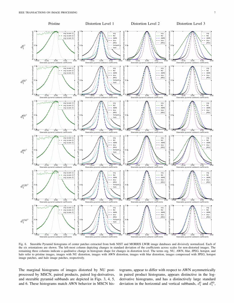
Fig. 6. Steerable Pyramid histograms of center patches extracted from both NIST and MORRIS LWIR image databases and divisively normalized. Each ofthe six orientations are shown. The left-most column depicting changes in standard deviation of the coefficients across scales for non-distorted images. Theremaining three columns indicate a qualitative change in histogram shape for changes in distortion level. The terms org, NU, AWN, blur, JPEG, hotspot, andhalo refer to pristine images, images with NU distortion, images with AWN distortion, images with blur distortion, images compressed with JPEG, hotspotimage patches, and halo image patches, respectively.

The marginal histograms of images distorted by NU post-processed by MSCN, paired products, paired log-derivatives,and steerable pyramid subbands are depicted in Figs. 3, 4, 5,and 6. These histograms match AWN behavior in MSCN his-

tograms, appear to differ with respect to AWN asymmetricallyin paired product histograms, appears distinctive in the log-derivative histograms, and has a distinctively large standarddeviation in the horizontal and vertical subbands, d0

1 and d901 ,


of the steerable pyramid.The “Halo Effect” occurs naturally in the images in the OSU

database. Davis’s method [37], which is based on backgroundsubtraction and morphological techniques, was used to isolatemoving objects (often people) in the images. Since not allobjects extracted using this method exhibited the “Halo Ef-fect,” patches with a clear visible “Halo Effect” were isolatedby hand. A total of 188 example patches were thus selectedfrom the OSU database for use here. The marginal histogramscomputed from MSCN coefficients exhibit a slight skew inFig. 3, the paired product and paired log-derivative coefficientsexhibit heavier tails in Figs. 4 and 5, and the steerable pyramidcoefficients exhibit fatter histograms as depicted in Fig. 6.These histogram comparisons may not only reflect the “HaloEffect” in isolation since these artifacts are combined with thenon-linearity associated with Ferro-Electric sensors.

Hotspots were isolated by hand from the NIST and MOR-RIS databases. A total of 135 hotspot patches including peo-ple, environmental hazards, and other miscellaneous objectswere extracted. When comparing to the natural LWIR imagehistrograms, the hotspot histogram shapes computed usingMSCN coefficients demonstrate an asymmetry in Fig. 3, pairedproduct and paired log-derivative coefficients exhibit peakinessin Figs. 4 and 5, and steerable pyramid coefficients exhibitheavier tails in Fig. 6.

JPEG, Additive White Noise (AWN), and blur distortionswere compared using the same set of images drawn fromthe NIST and MORRIS databases. JPEG images were gen-erated at the 100, 90, and 80 percent quality settings cor-responding to distortion levels 1, 2, and 3 producing aver-age respective bit rates of 3.6, 1.0, and 0.5 bpp. Distortionlevels involving Gaussian white noise matched the levels ofNU mentioned previously for comparability, using σAWN ={0.0025, 0.01375, 0.025} (recall the gray-scale range is [0, 1]).Blur was generated with a Gaussian blur kernel with scaleparameters σb = {1, 2, 3}.

JPEG distortions cause the MSCN, paired product, pairedlog-derivative, and steerable pyramid histograms to becomenarrower. These same histograms for AWN become wider.Blur distortion histograms become narrower as in JPEG, withthe exception of the steerable pyramid histograms.

C. Feature Models

A parametric General Gaussian Distribution (GGD) [38] hasbeen used to model the MSCN, Paired Log-Derivative, andsteerable pyramid subband coefficients. The associated GGDprobability density function is

f(x;α, σ2) =α

2βΓ(1/α)exp

(−( |x|β

)α)where

Γ (x) =

∞∫0

sx−1e−sds.

An Asymmetric Gaussian Distribution (AGGD) [39] hasbeen used to effectively model to the paired product coeffi-

−3.0 −2.5 −2.0 −1.5 −1.0 −0.5 0.0 0.5 1.0 1.5

Component 1

−8

−6

−4

−2

0

2

4

6

8

Com

pone

nt2

orgNUAWNblurJPEGhalo

Fig. 7. A total of 46 features over 3 scales yields 138 features per image,projected here into 2 dimensional space using PCA. Even though the totalexplained variance ratio of top two components is 0.734, distorted imagescluster away from the natural images. Note that hotspots were not included inthe projection because they significantly produce a sparse distribution likelyresulting from the limited size of the image patches.

cients. The pdf is

f(x; v, σ2l , σ

2r) =

v

(βl+βr)Γ( 1v )exp

(−(−xβl

)v)x < 0

v(βl+βr)Γ( 1

v )exp

(−(xβr

)v)x ≥ 0

where βl and βr are given by

βl = σl

√Γ(

1v

)Γ(

3v

)and

βr = σr

√Γ(

1v

)Γ(

3v

)respectively.

The parameters (α, σ2) of the GGD model fit can be esti-mated using the technique described in [38]. The parameters(v, σ2

l , σ2r ) of the AGGD model fits can be estimated using

the moment matching technique described in [39]. Anotherparameter, η, given by

η = (βr − βl)Γ(

2v

)Γ(

1v

)is also computed for each product image using the estimatesof the other parameters. Therefore, the best-fit model of eachset of paired product coefficients yields 4 features (η, v, σ2

l ,σ2r ).Since the hotspot images exhibit asymmetric histograms,

negative and positive MSCN coefficients were measured sep-arately. Negative and positive coefficients correspond to theleft and right halves of the histograms. Therefore, four pa-rameters (αl, σ2

l , αr, and σ2r ) were extracted from the MSCN

coefficients. The differences in value between the left and righthalves, αr−αl and σr−σl, are used to capture the asymmetry.A overview of the MSCN (f ), paired product (pp), paired log-


TABLE IIFEATURE SUMMARY FOR MSCN (f ), PAIRWISE PRODUCTS (pp), PAIRED LOG-DERIVATIVES (pd), AND STEERABLE PYRAMID SUBBANDS (sp) FOR THE

FIRST SCALE

Feature ID Feature Description Computation Proceduref1 - f2 Shape and Variance GGD fit to MSCN coefficientsf3 - f4 Shape and Variance difference GGD fit to right and left halves of MSCN coefficients

pp1 - pp4 Shape, mean, left variance, right variance AGGD fit to H pairwise productspp5 - pp8 Shape, mean, left variance, right variance AGGD fit to V pairwise productspp9 - pp12 Shape, mean, left variance, right variance AGGD fit to D1 pairwise productspp13 - pp16 Shape, mean, left variance, right variance AGGD fit to D2 pairwise productspd1 - pd2 Shape and Variance GGD fit to PD1 pairwise log-derivativepd3 - pd4 Shape and Variance GGD fit to PD2 pairwise log-derivativepd5 - pd6 Shape and Variance GGD fit to PD3 pairwise log-derivativepd7 - pd8 Shape and Variance GGD fit to PD4 pairwise log-derivativepd9 - pd10 Shape and Variance GGD fit to PD5 pairwise log-derivativepd11 - pd12 Shape and Variance GGD fit to PD6 pairwise log-derivativepd13 - pd14 Shape and Variance GGD fit to PD6 pairwise log-derivativesp1 - sp2 Shape and Variance GGD fit to d0

◦1 subband

sp3 - sp4 Shape and Variance GGD fit to d30◦

1 subbandsp5 - sp6 Shape and Variance GGD fit to d60

◦1 subband


1 subbandsp9 - sp10 Shape and Variance GGD fit to d120

◦1 subband


1 subband

derivative (pd), and steerable pyramid subband (sp) featuresis provided in Table II.

To visualize the clustering of the features over three scales,the features for each distortion class were projected into atwo-dimensional space using Principle Component Analysis(PCA) as depicted in Fig. 7. The distorted images appear tocluster in this projection which reasonably preserves their classgroupings.

A boxplot comparing the features in Table II betweenpristine LWIR images and pristine visible light images isprovided in Fig. 8. A total of 29 pristine visible light imageswere obtained from the LIVE Image Quality AssessmentDatabase [40] [41] [42]. The MSCN shape parameter, f1, isnot significantly different between visible and LWIR imageswhen using 95 percent confidence intervals. Comparing f3,we can infer that LWIR images provide more symmetricallyshaped MSCN histograms with 95 percent confidence.

The mean parameter, η, for each of the paired productfeatures differs between LWIR and visible light images. Ad-ditionally most of the standard deviation parameters, σl andσr, differ between the modalities. Most shape parametersfor paired products do not appear to differ between LWIRand visible light images. By contrast, most of the shapesand standard deviation parameters for pd and sp are signifi-cantly different from visible light images. Note that individualparameter differences are bound to exist by chance with alow number of pristine images, but there does seem to be adifference between the two groups overall.

D. NIST Descriptors

Previous work by NIST has produced four Image QualityIndicators (IQIs) [3] [4] [5] which are described as Bright-ness (B), Contrast (C), Spatial Resolution (SR), and Non-Uniformity (NU) defined as

f 1 f 2 f 3 f 4

−1

0

1

2

3

4

Para

met

erV

alue

MSCN features (f )

LWIRVisible Light

pp1

pp2

pp3

pp4

pp5

pp6

pp7

pp8

pp9

pp10

pp11

pp12

pp13

pp14

pp15

pp16

−0.2

0.0

0.2

0.4

0.6

0.8

1.0

1.2

Para

met

erV

alue

paired product features (pp)pd

1

pd2

pd3

pd4

pd5

pd6

pd7

pd8

pd9

pd10

pd11

pd12

pd13

pd14

0.5

1.0

1.5

2.0

Para

met

erV

alue

paired log-derivative features (pd)

sp1

sp2

sp3

sp4

sp5

sp6

sp7

sp8

sp9

sp10

sp11

sp12

0.0

0.5

1.0

1.5

2.0

2.5

3.0

Para

met

erV

alue

steerable pyramid subband (sp)

Fig. 8. Box plot comparison of features between natural LWIR and naturalvisible light images. The notches indicate 95 percent confidence intervalsabout the median.

• B is the average of the luminosity intensities:

B =1

MN

∑i∈N

∑j∈M

I(i, j)

• C is defined as RMS contrast:

C =

√1

MN

∑i∈N

∑j∈M

(I(i, j)−B)2

• SR (cycles/pixel) is computed by

SR =

∫ fc

0

(MTFcurve(u)− NEM) du

where MTFcurve(u) is the modulation transfer function


defined by the Butterworth filter

H(u) = 1/

(1 +

(u

Wn

)4)

of order 2. The cutoff frequency is

fc = Wn [(1− NEM) /NEM]0.25

where NEM = 0.02861 is the Noise Equivalent Modula-tion.

• NU is given by NU = µ/σ = B/C, the SNR of theimage.

As currently defined, the SR statistic, which depends di-rectly on the parameter Wn, is not implementable. Thisdependency on Wn assumes that any loss of spatial resolutioncan be modeled based on the response of a Butterworthfilter. According to Morris et al. [31], the log of the radialspectral power of LWIR images can be well described asfollowing a GGD probability law. Unfortunately, this fit doesnot generalize when distortions are present in an image, thusa 10th order polynomial approximation was used to yield amuch better fit. Overall, the IQIs provide a total of 13 featuresthat are extracted from each image. Unlike the other features,the IQI features are not model based, but rather are samplestatistics.

III. TASKING ON NSSIn this section, we study the practical usefulness of the

LWIR NSS and IQI features just described for solving fivedifferent visual LWIR tasks. First, we use the features todevelop a measure of NU on LWIR images. Second, we devisea method to determine presence of the “Halo Effect.” The thirdtask is automated prediction of the ability of human experts todetect targets of interest on LWIR images. Fourth, we describea human study which to obtain subjective quality scores onLWIR images, and show that the NSS features are highlypredictive of subjective image quality. Lastly, we will showhow the LWIR NSS can be used to create localized distortionmaps which can aid the identification of local distortions suchas hotspots and occurrences of the “Halo Effect.”

A. Measuring NU

In NUC algorithms, producing a no-reference estimate ofthe NU in an image is essential [17]. State-of-the-art methodsfor estimating the magnitude of NU include the Roughnessindex, Effective Roughness Index, and SNR. LWIR imagescommonly contain both fixed pattern noise and additive whitenoise, and the level of both types of noise should be estimated.

The most common method for estimating NU is the spatialSNR of the image defined as µ/σ where σ and µ are thestandard deviation and mean pixel intensities within a user-defined area. Another common and popular method is theRoughness [43] index:

Ro(I) =‖h1 ∗ I‖1 + ‖h2 ∗ I‖1

‖I‖1where h1 is the 1-D differencing filter with impulse response[1,−1], h2 = h1

T , and ‖ · ‖1 is the L1 norm. The Effective

1 2 3 4 1 2 3 4 5 6 7 8 9 10 11 12 13 14 15 16 1 2 3 4 5 6 7 8 9 10 11 12 13 14 1 2 3 4 5 6 7 8 9 10 11 12

0.0

0.2

0.4

0.6

0.8

1.0

SRC

C

ff pppp pdpd spsp

AWNNUH

NUV

NUHV

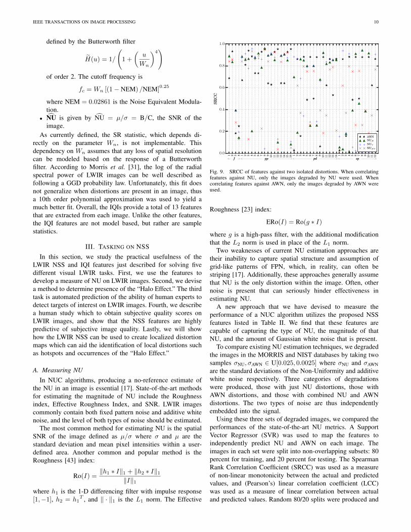
Fig. 9. SRCC of features against two isolated distortions. When correlatingfeatures against NU, only the images degraded by NU were used. Whencorrelating features against AWN, only the images degraded by AWN wereused.

Roughness [23] index:

ERo(I) = Ro(g ∗ I)

where g is a high-pass filter, with the additional modificationthat the L2 norm is used in place of the L1 norm.

Two weaknesses of current NU estimation approaches aretheir inability to capture spatial structure and assumption ofgrid-like patterns of FPN, which, in reality, can often bestriping [17]. Additionally, these approaches generally assumethat NU is the only distortion within the image. Often, othernoise is present that can seriously hinder effectiveness inestimating NU.

A new approach that we have devised to measure theperformance of a NUC algorithm utilizes the proposed NSSfeatures listed in Table II. We find that these features arecapable of capturing the type of NU, the magnitude of thatNU, and the amount of Gaussian white noise that is present.

To compare existing NU estimation techniques, we degradedthe images in the MORRIS and NIST databases by taking twosamples σNU, σAWN ∈ U[0.025, 0.0025] where σNU and σAWNare the standard deviations of the Non-Uniformity and additivewhite noise respectively. Three categories of degradationswere produced, those with just NU distortions, those withAWN distortions, and those with combined NU and AWNdistortions. The two types of noise are thus independentlyembedded into the signal.

Using these three sets of degraded images, we compared theperformances of the state-of-the-art NU metrics. A SupportVector Regressor (SVR) was used to map the features toindependently predict NU and AWN on each image. Theimages in each set were split into non-overlapping subsets: 80percent for training, and 20 percent for testing. The SpearmanRank Correlation Coefficient (SRCC) was used as a measureof non-linear monotonicity between the actual and predictedvalues, and (Pearson’s) linear correlation coefficient (LCC)was used as a measure of linear correlation between actualand predicted values. Random 80/20 splits were produced and


TABLE IIIPREDICTING FOREGROUND AWN WITH BACKGROUND DISTORTION. SRCC AND LCC MEASURED OVER 1000 ITERATIONS USING 80/20 TRAIN/TESTSPLITS. “NONE” INDICATES NO BACKGROUND DISTORTION, NUH INDICATES PRESENCE OF HORIZONTAL STRIPING NU BACKGROUND DISTORTIONS,

NUV INDICATES PRESENCE OF VERTICAL STRIPING NU BACKGROUND DISTORTIONS, AND NUHV INDICATES PRESENCE OF GRID-LIKE NUBACKGROUND DISTORTIONS. L1 AND L2 REFERS TO L1 AND L2 NORMS RESPECTIVELY. THE IQIS WERE USED IN PLACE OF SNR BECAUSE SNR

ALONE PERFORMED EXTREMELY POORLY.

NR Method SRCC LCCNone NUH NUV NUHV None NUH NUV NUHV

f + pp+ pd+ sp 0.974 0.966 0.964 0.966 0.977 0.969 0.967 0.969f + pp+ pd 0.975 0.964 0.966 0.965 0.977 0.967 0.969 0.969f + pp 0.972 0.960 0.960 0.961 0.975 0.963 0.963 0.965f + pd 0.969 0.955 0.957 0.960 0.972 0.959 0.960 0.963f 0.963 0.950 0.952 0.954 0.966 0.953 0.957 0.958pp 0.967 0.962 0.961 0.961 0.971 0.965 0.965 0.965pd 0.955 0.948 0.953 0.948 0.959 0.953 0.956 0.952sp 0.957 0.964 0.955 0.957 0.957 0.960 0.952 0.956Ro, L1 0.697 0.504 0.499 0.509 0.747 0.571 0.569 0.578Ro, L2 0.714 0.567 0.556 0.593 0.718 0.583 0.565 0.600ERo, L1 0.651 0.709 0.703 0.663 0.693 0.761 0.756 0.702ERo, L2 0.795 0.695 0.619 0.736 0.786 0.693 0.609 0.710IQIs 0.601 0.653 0.615 0.629 0.589 0.637 0.603 0.612

TABLE IVPREDICTING FOREGROUND NU WITH BACKGROUND DISTORTION. SRCC AND LCC MEASURED OVER 1000 ITERATIONS USING 80/20 TRAIN/TEST

SPLITS. NUH REFERS TO HORIZONTAL STRIPING NU FOREGROUND DISTORTIONS, NUV REFERS TO VERTICAL STRIPING NU FOREGROUNDDISTORTIONS, AND NUHV REFERS TO GRID-LIKE NU FOREGROUND DISTORTIONS. “NONE” REFERS TO ABSENCE OF BACKGROUND DISTORTION, AND“AWN” REFERS TO PRESENCE OF AWN BACKGROUND DISTORTION. L1 AND L2 REFERS TO L1 AND L2 NORMS RESPECTIVELY. THE IQIS WERE USED

IN PLACE OF SNR BECAUSE SNR PERFORMED EXTREMELY POORLY.

NR MethodSRCC LCC

NUH NUV NUHV NUH NUV NUHVNone AWN None AWN None AWN None AWN None AWN None AWN

f + pp+ pd+ sp 0.975 0.973 0.970 0.969 0.977 0.969 0.976 0.973 0.972 0.971 0.978 0.969f + pp+ pd 0.975 0.973 0.969 0.969 0.977 0.969 0.976 0.972 0.971 0.969 0.978 0.970f + pp 0.971 0.973 0.964 0.967 0.977 0.973 0.972 0.972 0.966 0.966 0.978 0.975f + pd 0.967 0.938 0.961 0.940 0.971 0.923 0.968 0.939 0.964 0.944 0.973 0.919f 0.940 0.897 0.949 0.895 0.951 0.866 0.942 0.888 0.951 0.891 0.952 0.851pp 0.970 0.972 0.966 0.969 0.976 0.975 0.971 0.972 0.968 0.968 0.977 0.976pd 0.961 0.930 0.957 0.939 0.965 0.916 0.962 0.932 0.959 0.942 0.966 0.916sp 0.961 0.964 0.967 0.965 0.973 0.965 0.962 0.963 0.966 0.966 0.973 0.962Ro, L1 0.548 0.157 0.552 0.151 0.556 0.136 0.626 0.239 0.621 0.236 0.625 0.229Ro, L2 0.572 0.213 0.609 0.244 0.548 0.183 0.533 0.237 0.575 0.274 0.502 0.212ERo, L1 0.424 0.400 0.404 0.393 0.464 0.268 0.417 0.414 0.404 0.413 0.468 0.328ERo, L2 0.565 0.191 0.642 0.336 0.646 0.222 0.565 0.283 0.678 0.401 0.647 0.308IQIs 0.005 0.140 0.004 0.108 0.025 0.061 0.004 0.127 0.006 0.086 0.024 0.041

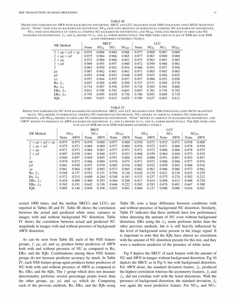
scored 1000 times, and the median SRCCs and LCCs arereported in Tables III and IV. Table III shows the correlationbetween the actual and predicted white noise variance inimages with and without background NU distortion. TableIV shows the correlation between actual and predicted NUmagnitude in images with and without presence of backgroundAWN distortion.

As can be seen from Table III, each of the NSS featuregroups, f , pp, pd, and sp, produce better predictors of AWNboth with and without presence of NU as compared to Ro,ERo, and the IQIs. Combinations among these NSS featuregroups do not increase predictor accuracy by much. In TableIV, each NSS feature group again produces better predictors ofNU both with and without presence of AWN as compared toRo, ERo, and the IQIs. The f group which does not measuredirectionality performs several percentage points lower thanthe other groups, pp, pd, and sp, which do. Comparingeach of the previous methods, Ro, ERo, and the IQIs using

Table III, note a large difference between conditions withand without presence of background NU distortion. Similarly,Table IV indicates that these methods have low performancewhen detecting the amount of NU even without backgrounddistortion. ERo using the L2 norm performs better than theother previous methods, but it is still heavily influenced bythe level of background noise present in the image signal. Itis important to note that the IQIs have almost no correlationwith the amount of NU distortion present for this test, and theywere a mediocre predictor of the presence of white noise.

Fig 9 depicts the SRCC of each feature with the amount ofNU and AWN in images without background distortion. Fig 10depicts the SRCC as in Fig 9, but with background distortion.For AWN alone, the standard deviation feature, f2, producedthe highest correlation whereas the asymmetry features, f3 andf4, did not correlate well with the listed distortions. With thepresence of background distortion, the standard deviation, f2

was again the most predictive feature. For NUH and NUV


1 2 3 4 1 2 3 4 5 6 7 8 9 10 11 12 13 14 15 16 1 2 3 4 5 6 7 8 9 10 11 12 13 14 1 2 3 4 5 6 7 8 9 10 11 12

0.0

0.2

0.4

0.6

0.8

1.0

SRC

C

ff pppp pdpd spsp

AWNNUH

NUV

NUHV

Fig. 10. SRCC of features against two combined distortions. Whencorrelating features against NU, the images degraded by both NU and AWNwere used. When correlating features against AWN, this same image set wasused.

with and without background distortion, the shape parameterf1 was the best predictor.

Since NUH and NUV are striping effects, they are highlyoriented distortions. The sp group features show significantcorrelation with directionality, with vertical striping effectsbeing highly correlated with the d0

1 subband standard devi-ation, and horizontal striping effects being highly correlatedwith the d90

1 subband standard deviation. The paired productfeatures indicate a similar oriented correlation, the horizontalpaired product σr, pp4, correlates highly with vertical striping,and the vertical paired product σr, pp8, correlates highly withhorizontal striping. This high degree of correlation betweenpredicted and actual degree of distortion in single features isuseful.

B. Discriminating the “Halo Effect”

The authors of [28] developed a person-detector whichused the statistical gradients of estimated halos to enhancethe detection task. To our knowledge, no methods exist fordetecting halo artifacts in LWIR images.

To study how well the “Halo Effect” can be discriminatedusing our feature models, two sets of image patches (with andwithout halos) were constructed using background subtractionand manual classification to develop a supervised learner. Mostof the image patches were of size 110x110. A total of 415image patches were contained in both sets, with 227 imagepatches being halo-free, and 188 patches containing halos.

AWN and NU distortions were applied to each patch inboth sets to reduce the dependence on the correlation between“Halo Effect” and the level of other common noise distortions.Each of these 415 image patches thus contained two artificialdistortions in addition to the halo effect distortions. The distor-tion magnitudes σNU, σAWN ∈ U[0.0025, 0.025] were randomlysampled and used as the variance of the white noise and Non-Uniformity distortions for each patch. The intervals for thisuniform distribution were selected to scale the distortion froma just-noticeable to a significant difference.

0.0 0.2 0.4 0.6 0.8 1.0

False Positive Rate

0.0

0.2

0.4

0.6

0.8

1.0

Tru

ePo

siti

veR

ate

f + pp + pd + sp

f + pp + pd

f + pp

f + pd

f

pp

pd

sp

IQIs

Fig. 11. ROC indicating the ability of NR algorithms to sort patches aseither containing halos or as non-halo patches. Curves computed from 1000train/test iterations using 415 total patches from the OSU dataset withoutcontent overlap.

TABLE VAREAS UNDER THE ROC CURVES IN FIG. 11

NR Feature Set Area Under ROC Curvef + pp+ pd+ sp 0.795f + pp+ pd 0.711f + pp 0.723f + pd 0.675f 0.651pp 0.699pd 0.639sp 0.795IQIs 0.735

Given these two distorted sets, those containing halos andthose without, we devised a binary classification task. Asin section A, we split the dataset into two non-overlappingsubsets: 80 percent for training and 20 percent for testing. ASupport Vector Classifier (SVC) was used to map the featuresbetween two classes. Random 80/20 splits were producedand classified with associated class probability estimates 1000times.

Receiver Operating Characteristic (ROC) curves for the bi-nary classification task using the proposed feature groups andthe IQIs are shown in Fig. 11. The areas under the ROC curvesare provided in Table V. The proposed NSS-based featuregroups, except for sp and combinations of sp, achieved worseperformance as compared to the IQIs for this discriminationtask. Specifically, the sp performed significantly above theIQIs providing the largest discrimination capability both aloneand when combined with with f , pp, and pd feature groups.

The steerable pyramid transform provides directionality ofdistortion which provides a great deal of information espe-cially for the provided halo effect patches. Most objects in ascene are not circularly symmetric, thus their associated haloeffect will not be symmetric. The steerable pyramid providessmooth directional features which are highly useful for thetask.


TABLE VIMEDIAN SRCC AND LCC BETWEEN ACTUAL AND PREDICTED TTP FROM

1000 ITERATIONS

NR Feature Set SRCC LCCf + pp+ pd+ sp 0.665 0.671f + pp+ pd 0.640 0.646f + pp 0.582 0.601f + pd 0.609 0.613f 0.504 0.527pp 0.562 0.582pd 0.566 0.568sp 0.340 0.367IQIs 0.621 0.630

C. TTP of Firefighters and Hazards

Researchers at NIST conducted a study involving firefight-ers whose task was two-fold [4]. First, given an LWIR image,the expert determined whether a hazard was present. Second,if a hazard was present, the expert was asked to identifythe location of the hazard. This study was broken up intotwo phases. The phase 1 study used 4500 images. Theseimages were created by degrading 180 pristine images. Fivedifferent levels of degradation corresponding to each IQI weregenerated and 25 sets of the four IQIs were used (for atotal of 100 unique arrangements of the five values of eachof the four IQIs). These 25 sets were deemed sufficient torepresent the defined IQI space (54). Phase 2 used 55 sets ofthe four IQIs (for a total of 9900 images). The larger numberof sets served also to extend the range of IQIs to include moreextreme values. Note that the IQIs in this study were used asdistortion-generating settings, allowing for direct measurementof distortion with TTP.

In this study, the experts were given a stimulus image, andtasked to either identify the location of the environmentalhazard by clicking on it, or by indicating that there is nodistortion. To better isolate detectability, we converted thedataset into patches centered about the hazards. Images withno hazards were discarded. Next, only the scores of observersthat attempted to identify the location of the present envi-ronmental hazard were kept. Hits and misses were measureddepending on whether the cursor click was near the hazard.The probability of hit was computed over all observers. Bymodifying the dataset in this way, SRCC and LCC correlationsbetween target quality and target detectability could be moredirectly measured.

Using the probability of hit, the NSS quality features, andthe IQIs, we used a SVR to estimate TTP. As a way of compar-ing the features, the median SRCC and LCC coefficients arereported in VI from 1000 iterations. Combinations of featuresprovide the best estimators of TTP, with the combinationof all natural features providing the highest correlations forTTP. Note that the IQIs in VI use the 13 features, whilethe degradations to the images provided in the study mademodifications based on the original 4 parameters.

D. Blind Image Quality Assessment of LWIR Images

We conducted a lengthy and sizeable human study, theresults of which we used to assess how well NSS-based blind

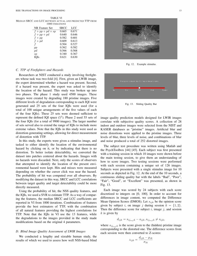
Fig. 12. Example stimulus

Fig. 13. Sliding Quality Bar

image quality prediction models designed for LWIR imagescorrelate with subjective quality scores. A collection of 28indoor and outdoor images were selected from the NIST andKASER databases as “pristine” images. Artificial blur andnoise distortions were applied to the pristine images. Threelevels of blur, three levels of noise, and combinations of blurand noise produced a total of 252 distorted images.

The subject test procedure was written using Matlab andthe PsychToolbox [44] [45]. Each subject was first presentedwith a training session in which 10 images were shown beforethe main testing session, to give them an understanding ofhow to score images. Two testing sessions were performedwith each session containing a unique set of 126 images.Subjects were presented with a single stimulus image for 10seconds as depicted in Fig. 12. At the end of the 10 seconds, acontinuous sliding quality bar with the labels “Bad”, “Poor”,“Fair”, “Good”, or “Excellent” was presented, as shown inFig. 13.

Each image was scored by 24 subjects with each scorediscretized to integers on [0, 100]. In order to account fordifferences in image content, we computed the DifferenceMean Opinion Scores (DMOS). Let sijk be the opinion scoregiven by subject i, on image j during session k = {1, 2}.Then the difference score for subject i, image j, and sessionk is given by

dijk = sijrefk − sijk, sijrefk 6= sijk,

where sijrefk is the score given to the (hidden) pristine imagecorresponding to the distorted one. The difference scores fromeach session were then converted to Z-scores:

zijk =dijk − µik

σik


0 20 40 60 80 100

DMOS

0

5

10

15

20

25

30

35N

umbe

rof

Imag

es

Fig. 14. Histogram of DMOS scores

where

µik =1

Nik

Nik∑j=1

dijk

and

σik =

√√√√ 1

Nik − 1

Nik∑j=1

(dijk − µik)2

and where Nik is the number of test images seen by subjecti in session k.

The subject rejection procedure specified in the ITU-RBT 500.11 recommendation is useful for discarding scoresfrom unreliable subjects. Z-scores are considered normallydistributed if their kurtosis falls between the values of 2 and4. The recommendation is to reject if more than 5 percent ofthe Z-scores lie outside two standard deviations of the mean.Using this procedure, all except one subject was found to beacceptable. The one outlier chose the same value of 50 for allimages. Thus only one subject was rejected [45] [46].

After the subject rejection procedure, the values of zijk fellinto a range on [−3, 3]. A linear rescaling was used to remapthe scores onto [0, 100] using

z′ij =100(zij + 3)

6

Finally the Difference Mean Opinion Score (DMOS) of eachimage was computed as the mean of the M = 24 rescaled Z-scores:

DMOSj =1

M

M∑i=1

z′ij .

A plot of the histogram of the DMOS scores is shown in Fig.14, indicating a reasonably broad distribution of the DMOSscores.

Table VII shows the Spearman’s Rank Correlation Coef-ficient (SRCC) and (Pearson’s) linear correlation coefficient(LCC) between the subjective scores and the model predictionsfor NR feature groups. The results were computed using 1000iterations of randomly sampled training and testing groups.As in the previous sections, 80 percent of the data is usedfor training and the remainder for testing. Care was taken

TABLE VIIMEDIAN SRCC AND LCC BETWEEN DMOS AND PREDICTED DMOS

MEASURED OVER 1000 ITERATIONS

NR Feature Set Median SRCC Median LCCf + pp+ pd+ sp 0.815 0.820f + pp+ pd 0.794 0.809f + pp 0.809 0.817f + pd 0.727 0.742f 0.714 0.736pp 0.794 0.809pd 0.696 0.732sp 0.825 0.828IQIs 0.726 0.705Ro, L1 0.135 0.189Ro, L2 0.162 0.221ERo, L1 0.570 0.576ERo, L2 0.616 0.667

1 2 3 4 1 2 3 4 5 6 7 8 9 10 11 12 13 14 15 16 1 2 3 4 5 6 7 8 9 10 11 12 13 14 1 2 3 4 5 6 7 8 9 10 11 12

0.0

0.2

0.4

0.6

0.8

1.0

SRC

C

ff pppp pdpd spsp

AWNblurboth

Fig. 15. SRCC of NSS features against DMOS scores. The performanceagainst each distortion (noise and blur) was isolated for the purposes ofcomparison.

to not overlap training and testing on the same content inany iteration since such an overlap could inflate performanceresults by training on the content rather than distortion. AnSVR was used to fit the NSS feature parameters to the DMOSscores.

We observe that the steerable pyramid group features pro-vide the highest correlation with the human subjective scoreswhich is only a slight improvement over the BRISQUE model,f + pp. The combinations of feature groups performs worsecompared to the individual groups indicating possible overfit-ting with the training set. For these blur and AWN distortions,the directional feature groups provide the highest correlationwith DMOS scores with the IQIs and NU distortion modelsproviding comparatively low correlation. The proposed modelsprovide a great deal of predictive capability with humanopinion scores, but there appears to be additional variationnot accounted for in our proposed models.

Fig 15 depicts the SRCC of each feature’s value withthe human opinion scores. The highest individual featurecorrelations occur in the paired Log-derivative feature group,pd, but VII indicates that individual feature correlations are notas powerful as groups of features for predicting quality scores.


In fact, the sp feature group provides the highest correlationswith DMOS scores when used together in a regression, butindividually, they appear to make poor predictors.

E. Local Distortion Maps

Local distortion maps can be useful for identifying localdistorted regions, which can occur as particular local dis-tortions such as hotspots or halos, or they may arise fromsome unknown (combination of) distortions. It is possible toautomatically find local distorted regions of LWIR imagesusing NSS-based features.

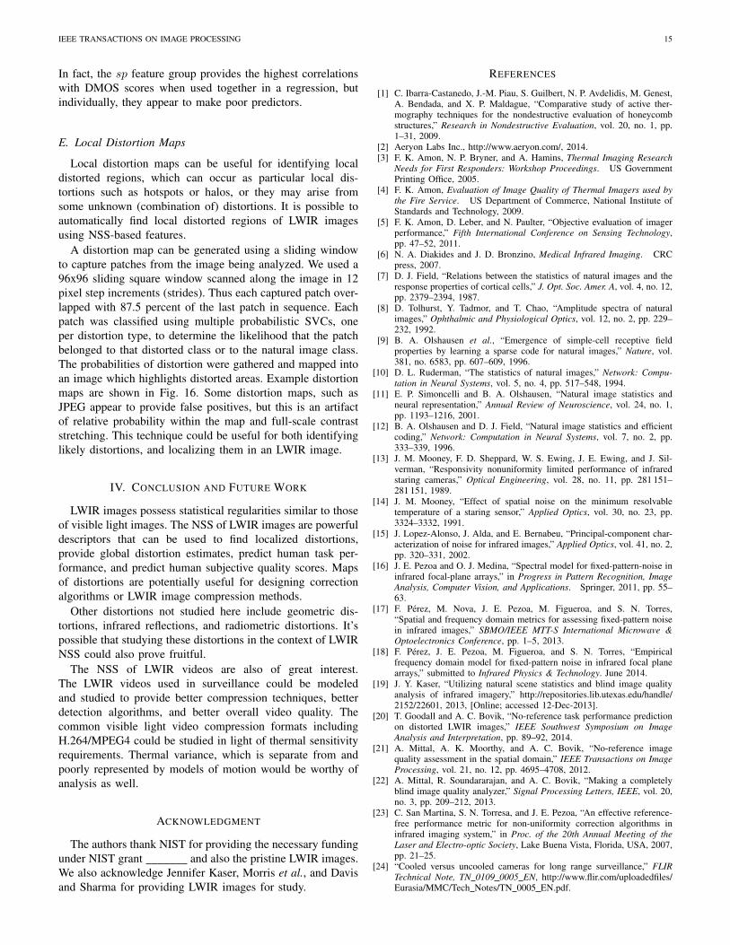
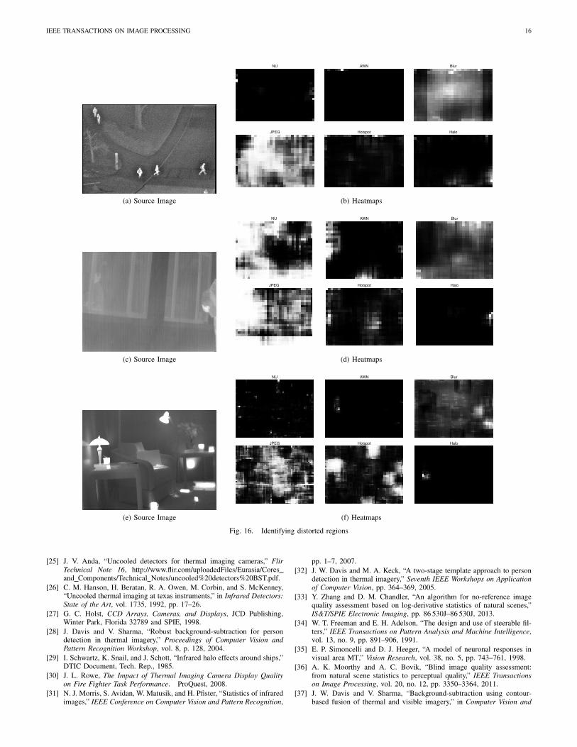
A distortion map can be generated using a sliding windowto capture patches from the image being analyzed. We used a96x96 sliding square window scanned along the image in 12pixel step increments (strides). Thus each captured patch over-lapped with 87.5 percent of the last patch in sequence. Eachpatch was classified using multiple probabilistic SVCs, oneper distortion type, to determine the likelihood that the patchbelonged to that distorted class or to the natural image class.The probabilities of distortion were gathered and mapped intoan image which highlights distorted areas. Example distortionmaps are shown in Fig. 16. Some distortion maps, such asJPEG appear to provide false positives, but this is an artifactof relative probability within the map and full-scale contraststretching. This technique could be useful for both identifyinglikely distortions, and localizing them in an LWIR image.

IV. CONCLUSION AND FUTURE WORK

LWIR images possess statistical regularities similar to thoseof visible light images. The NSS of LWIR images are powerfuldescriptors that can be used to find localized distortions,provide global distortion estimates, predict human task per-formance, and predict human subjective quality scores. Mapsof distortions are potentially useful for designing correctionalgorithms or LWIR image compression methods.

Other distortions not studied here include geometric dis-tortions, infrared reflections, and radiometric distortions. It’spossible that studying these distortions in the context of LWIRNSS could also prove fruitful.

The NSS of LWIR videos are also of great interest.The LWIR videos used in surveillance could be modeledand studied to provide better compression techniques, betterdetection algorithms, and better overall video quality. Thecommon visible light video compression formats includingH.264/MPEG4 could be studied in light of thermal sensitivityrequirements. Thermal variance, which is separate from andpoorly represented by models of motion would be worthy ofanalysis as well.

ACKNOWLEDGMENT

The authors thank NIST for providing the necessary fundingunder NIST grant and also the pristine LWIR images.We also acknowledge Jennifer Kaser, Morris et al., and Davisand Sharma for providing LWIR images for study.

REFERENCES

[1] C. Ibarra-Castanedo, J.-M. Piau, S. Guilbert, N. P. Avdelidis, M. Genest,A. Bendada, and X. P. Maldague, “Comparative study of active ther-mography techniques for the nondestructive evaluation of honeycombstructures,” Research in Nondestructive Evaluation, vol. 20, no. 1, pp.1–31, 2009.

[2] Aeryon Labs Inc., http://www.aeryon.com/, 2014.[3] F. K. Amon, N. P. Bryner, and A. Hamins, Thermal Imaging Research

Needs for First Responders: Workshop Proceedings. US GovernmentPrinting Office, 2005.

[4] F. K. Amon, Evaluation of Image Quality of Thermal Imagers used bythe Fire Service. US Department of Commerce, National Institute ofStandards and Technology, 2009.

[5] F. K. Amon, D. Leber, and N. Paulter, “Objective evaluation of imagerperformance,” Fifth International Conference on Sensing Technology,pp. 47–52, 2011.

[6] N. A. Diakides and J. D. Bronzino, Medical Infrared Imaging. CRCpress, 2007.

[7] D. J. Field, “Relations between the statistics of natural images and theresponse properties of cortical cells,” J. Opt. Soc. Amer. A, vol. 4, no. 12,pp. 2379–2394, 1987.

[8] D. Tolhurst, Y. Tadmor, and T. Chao, “Amplitude spectra of naturalimages,” Ophthalmic and Physiological Optics, vol. 12, no. 2, pp. 229–232, 1992.

[9] B. A. Olshausen et al., “Emergence of simple-cell receptive fieldproperties by learning a sparse code for natural images,” Nature, vol.381, no. 6583, pp. 607–609, 1996.

[10] D. L. Ruderman, “The statistics of natural images,” Network: Compu-tation in Neural Systems, vol. 5, no. 4, pp. 517–548, 1994.

[11] E. P. Simoncelli and B. A. Olshausen, “Natural image statistics andneural representation,” Annual Review of Neuroscience, vol. 24, no. 1,pp. 1193–1216, 2001.

[12] B. A. Olshausen and D. J. Field, “Natural image statistics and efficientcoding,” Network: Computation in Neural Systems, vol. 7, no. 2, pp.333–339, 1996.

[13] J. M. Mooney, F. D. Sheppard, W. S. Ewing, J. E. Ewing, and J. Sil-verman, “Responsivity nonuniformity limited performance of infraredstaring cameras,” Optical Engineering, vol. 28, no. 11, pp. 281 151–281 151, 1989.

[14] J. M. Mooney, “Effect of spatial noise on the minimum resolvabletemperature of a staring sensor,” Applied Optics, vol. 30, no. 23, pp.3324–3332, 1991.

[15] J. Lopez-Alonso, J. Alda, and E. Bernabeu, “Principal-component char-acterization of noise for infrared images,” Applied Optics, vol. 41, no. 2,pp. 320–331, 2002.

[16] J. E. Pezoa and O. J. Medina, “Spectral model for fixed-pattern-noise ininfrared focal-plane arrays,” in Progress in Pattern Recognition, ImageAnalysis, Computer Vision, and Applications. Springer, 2011, pp. 55–63.

[17] F. Perez, M. Nova, J. E. Pezoa, M. Figueroa, and S. N. Torres,“Spatial and frequency domain metrics for assessing fixed-pattern noisein infrared images,” SBMO/IEEE MTT-S International Microwave &Optoelectronics Conference, pp. 1–5, 2013.

[18] F. Perez, J. E. Pezoa, M. Figueroa, and S. N. Torres, “Empiricalfrequency domain model for fixed-pattern noise in infrared focal planearrays,” submitted to Infrared Physics & Technology. June 2014.

[19] J. Y. Kaser, “Utilizing natural scene statistics and blind image qualityanalysis of infrared imagery,” http://repositories.lib.utexas.edu/handle/2152/22601, 2013, [Online; accessed 12-Dec-2013].

[20] T. Goodall and A. C. Bovik, “No-reference task performance predictionon distorted LWIR images,” IEEE Southwest Symposium on ImageAnalysis and Interpretation, pp. 89–92, 2014.

[21] A. Mittal, A. K. Moorthy, and A. C. Bovik, “No-reference imagequality assessment in the spatial domain,” IEEE Transactions on ImageProcessing, vol. 21, no. 12, pp. 4695–4708, 2012.

[22] A. Mittal, R. Soundararajan, and A. C. Bovik, “Making a completelyblind image quality analyzer,” Signal Processing Letters, IEEE, vol. 20,no. 3, pp. 209–212, 2013.

[23] C. San Martina, S. N. Torresa, and J. E. Pezoa, “An effective reference-free performance metric for non-uniformity correction algorithms ininfrared imaging system,” in Proc. of the 20th Annual Meeting of theLaser and Electro-optic Society, Lake Buena Vista, Florida, USA, 2007,pp. 21–25.

[24] “Cooled versus uncooled cameras for long range surveillance,” FLIRTechnical Note, TN 0109 0005 EN, http://www.flir.com/uploadedfiles/Eurasia/MMC/Tech Notes/TN 0005 EN.pdf.

http://www.aeryon.com/

http://repositories.lib.utexas.edu/handle/2152/22601

http://repositories.lib.utexas.edu/handle/2152/22601

http://www.flir.com/uploadedfiles/Eurasia/MMC/Tech_Notes/TN_0005_EN.pdf

http://www.flir.com/uploadedfiles/Eurasia/MMC/Tech_Notes/TN_0005_EN.pdf


(a) Source Image

NU AWN Blur

JPEG Hotspot Halo

(b) Heatmaps

(c) Source Image

NU AWN Blur

JPEG Hotspot Halo

(d) Heatmaps

(e) Source Image

NU AWN Blur

JPEG Hotspot Halo

(f) Heatmaps

Fig. 16. Identifying distorted regions

[25] J. V. Anda, “Uncooled detectors for thermal imaging cameras,” FlirTechnical Note 16, http://www.flir.com/uploadedFiles/Eurasia/Coresand Components/Technical Notes/uncooled%20detectors%20BST.pdf.

[26] C. M. Hanson, H. Beratan, R. A. Owen, M. Corbin, and S. McKenney,“Uncooled thermal imaging at texas instruments,” in Infrared Detectors:State of the Art, vol. 1735, 1992, pp. 17–26.

[27] G. C. Holst, CCD Arrays, Cameras, and Displays, JCD Publishing,Winter Park, Florida 32789 and SPIE, 1998.

[28] J. Davis and V. Sharma, “Robust background-subtraction for persondetection in thermal imagery,” Proceedings of Computer Vision andPattern Recognition Workshop, vol. 8, p. 128, 2004.

[29] I. Schwartz, K. Snail, and J. Schott, “Infrared halo effects around ships,”DTIC Document, Tech. Rep., 1985.

[30] J. L. Rowe, The Impact of Thermal Imaging Camera Display Qualityon Fire Fighter Task Performance. ProQuest, 2008.

[31] N. J. Morris, S. Avidan, W. Matusik, and H. Pfister, “Statistics of infraredimages,” IEEE Conference on Computer Vision and Pattern Recognition,

pp. 1–7, 2007.[32] J. W. Davis and M. A. Keck, “A two-stage template approach to person

detection in thermal imagery,” Seventh IEEE Workshops on Applicationof Computer Vision, pp. 364–369, 2005.

[33] Y. Zhang and D. M. Chandler, “An algorithm for no-reference imagequality assessment based on log-derivative statistics of natural scenes,”IS&T/SPIE Electronic Imaging, pp. 86 530J–86 530J, 2013.

[34] W. T. Freeman and E. H. Adelson, “The design and use of steerable fil-ters,” IEEE Transactions on Pattern Analysis and Machine Intelligence,vol. 13, no. 9, pp. 891–906, 1991.

[35] E. P. Simoncelli and D. J. Heeger, “A model of neuronal responses invisual area MT,” Vision Research, vol. 38, no. 5, pp. 743–761, 1998.

[36] A. K. Moorthy and A. C. Bovik, “Blind image quality assessment:from natural scene statistics to perceptual quality,” IEEE Transactionson Image Processing, vol. 20, no. 12, pp. 3350–3364, 2011.

[37] J. W. Davis and V. Sharma, “Background-subtraction using contour-based fusion of thermal and visible imagery,” in Computer Vision and

http://www.flir.com/uploadedFiles/Eurasia/Cores_and_Components/Technical_Notes/uncooled%20detectors%20BST.pdf

http://www.flir.com/uploadedFiles/Eurasia/Cores_and_Components/Technical_Notes/uncooled%20detectors%20BST.pdf


Image Understanding, vol. 106, no. 2. Elsevier, 2007, pp. 162–182.[38] K. Sharifi and A. Leon-Garcia, “Estimation of shape parameter for

generalized gaussian distributions in subband decompositions of video,”IEEE Transactions on Circuits and Systems for Video Technology, vol. 5,no. 1, pp. 52–56, 1995.

[39] N.-E. Lasmar, Y. Stitou, and Y. Berthoumieu, “Multiscale skewed heavytailed model for texture analysis,” IEEE International Conference onImage Processing, pp. 2281–2284, 2009.

[40] H. R. Sheikh, Z. Wang, L. Cormack, and A. C. Bovik, “Live image qual-ity assessment database release 2,” http://live.ece.utexas.edu/research/quality.

[41] H. R. Sheikh, M. F. Sabir, and A. C. Bovik, “A statistical evaluationof recent full reference image quality assessment algorithms,” IEEETransactions on Image Processing, vol. 15, no. 11, pp. 3440–3451, 2006.

[42] Z. Wang, A. C. Bovik, H. R. Sheikh, and E. P. Simoncelli, “Imagequality assessment: from error visibility to structural similarity,” IEEETransactions on Image Processing, vol. 13, no. 4, pp. 600–612, 2004.

[43] M. M. Hayat, S. N. Torres, E. Armstrong, S. C. Cain, and B. Ya-suda, “Statistical algorithm for nonuniformity correction in focal-planearrays,” Applied Optics, vol. 38, no. 5, pp. 772–780, 1999.

[44] D. H. Brainard, “The psychophysics toolbox,” Spatial Vision, vol. 10,pp. 433–436, 1997.

[45] K. Seshadrinathan, R. Soundararajan, A. C. Bovik, and L. K. Cormack,“Study of subjective and objective quality assessment of video,” IEEETransactions on Image Processing, vol. 19, no. 6, pp. 1427–1441, 2010.

[46] ITU-R, “Recommendation BT.500-11. methodology for the subjectiveassessment of the quality of television pictures,” International Telecom-munication Union, Geneva, Switzerland, 2002.

Todd Richard Goodall received the B.S. degreein Computer Engineering from Clemson University,Clemson, SC, in May 2012. He joined the Labo-ratory for Image and Video Engineering (LIVE) inAugust 2013, and is currently pursuing the M.S. andPh.D. degrees in electrical and computer engineer-ing.

He is the recipient of the NDIA UWD AcademicFellowship for 2012-2013. His research interests in-clude the statistical modeling of images and videos,design of image and video quality assessment algo-

rithms, visual perception, and computational vision.

Alan Conrad Bovik holds the Cockrell FamilyEndowed Regents Chair in Engineering at The Uni-versity of Texas at Austin, where he is Director ofthe Laboratory for Image and Video Engineering(LIVE). He is a faculty member in the Departmentof Electrical and Computer Engineering and theInstitute for Neuroscience. His research interestsinclude image and video processing, computationalvision, and visual perception. He has published over700 technical articles in these areas and holds severalU.S. patents. His publications have been cited more

than 35,000 times in the literature, his current H-index is over 70, and he islisted as a Highly-Cited Researcher by Thompson Reuters. His several booksinclude the companion volumes The Essential Guides to Image and VideoProcessing (Academic Press, 2009).

Dr. Bovik has received a number of major awards from the IEEE SignalProcessing Society, including: the Society Award (2013); the TechnicalAchievement Award (2005); the Best Paper Award (2009); the Signal Pro-cessing Magazine Best Paper Award (2013); the Education Award (2007);the Meritorious Service Award (1998) and (co-author) the Young AuthorBest Paper Award (2013). He also was named recipient of the HonoraryMember Award of the Society for Imaging Science and Technology for 2013,received the SPIE Technology Achievement Award for 2012, and was theIS&T/SPIE Imaging Scientist of the Year for 2011. He is also a recipient ofthe Hocott Award for Distinguished Engineering Research from the CockrellSchool of Engineering at The University of Texas at Austin (2008) and theDistinguished Alumni Award from the University of Illinois at Champaign-Urbana (2008). He is a Fellow of the IEEE, the Optical Society of America(OSA), and the Society of Photo-Optical and Instrumentation Engineers(SPIE). He co-founded and was the longest-serving Editor-in-Chief of theIEEE Transactions on Image Processing (1996-2002), created and served asthe General Chairman of the First IEEE International Conference on ImageProcessing, held in Austin, Texas, in November, 1994, along with numerousother professional society activities, including: Board of Governors, IEEESignal Processing Society, 1996-1998;; Editorial Board, The Proceedings ofthe IEEE, 1998-2004; and Series Editor for Image, Video, and MultimediaProcessing, Morgan and Claypool Publishing Company, 2003-present.

Dr. Bovik is a registered Professional Engineer in the State of Texas andis a frequent consultant to legal, industrial and academic institutions.

Nicholas G. Paulter Jr. is the Group Leader forthe Security Technologies Group and is a formerProgram Manager for the Detection, Enforcement,and Inspection program of the Law EnforcementStandards Office (OLES) at NIST in Gaithersburg,MD. He develops and oversees metrology programsrelated to concealed-weapon detection, through-wallsurveillance, traffic control devices, imaging for se-curity and emergency response applications, biomet-rics for identification, and weapon output charac-terization. In this role, he has initiated two NIST

programs in sub-millimeter-wave concealed weapon imaging, facilitated thedevelopment of visible-light hyper-spectral image projection, initiated a NIST-centric imaging metrology program for security and emergency applications,started two through-wall surveillance/sensing metrology activities, and starteda program for characterization of the high-voltage output of electroshockweapons. He was awarded a NIST Bronze Medal in 2003 for his work indeveloping minimum performance requirements for metal detectors. Prior tobeing a Program Manager in OLES, from 1990 to 2005, Mr. Paulter was theLeader for the High-Speed Pulse Metrology Project at NIST. In that capacity,he developed several high-speed electrical pulse generation and samplingsystems, electro-optic based measurement systems, and short optical pulselaser systems for use in pulse metrology. Moreover, during his tenure as theProject Leader, the metrology services provided by his project became thebest in the world.

From 1980 to 1989, Mr. Paulter was with Los Alamos National Laboratory,Los Alamos, NM, and was involved in the study of fast electrical and opticalphenomena. Mr. Paulter has authored or co-authored over 100 peer-reviewedtechnical articles and provided numerous presentations at a variety of technicalconferences. He is a 2008-2009 Commerce Science and Technology Fellowand a 2010 IEEE Fellow; and received a B.S. in biological sciences from theUniversity of California, Santa Barbara in 1980; an M.S. in chemistry fromthe University of New Mexico in 1988; and an M.S. in electronics engineeringfrom the University of Colorado Boulder in 1990.

http://live.ece.utexas.edu/research/quality

http://live.ece.utexas.edu/research/quality

Documents

IEEE TRANSACTIONS ON IMAGE PROCESSING 1 Tasking on …live.ece.utexas.edu/research/IR/LWIR_TIP.pdf · IEEE TRANSACTIONS ON IMAGE PROCESSING 1 Tasking on Natural Statistics of Infrared