IEEE TRANSACTIONS ON IMAGE PROCESSING 1

Motion Tuned Spatio-temporal Quality Assessmentof Natural Videos

Kalpana Seshadrinathan*,Member, IEEEand Alan C. Bovik,Fellow, IEEE

Abstract—There has recently been a great deal of interest in thedevelopment of algorithms that objectively measure the integrityof video signals. Since video signals are being delivered tohumanend users in an increasingly wide array of applications andproducts, it is important that automatic methods of video qualityassessment (VQA) be available that can assist in controllingthe quality of video being delivered to this critical audience.Naturally, the quality of motion representation in videos playsan important role in the perception of video quality, yet existingVQA algorithms make little direct use of motion information ,thus limiting their effectiveness. We seek to ameliorate thisby developing a general, spatio-spectrally localized multiscaleframework for evaluating dynamic video fidelity that integr atesboth spatial and temporal (and spatio-temporal) aspects ofdistortion assessment. Video quality is evaluated not onlyin spaceand time, but also in space-time, by evaluating motion qualityalong computed motion trajectories. Using this framework,wedevelop a full reference VQA algorithm for which we cointhe term the MOtion-based Video Integrity Evaluation index,or MOVIE index. It is found that the MOVIE index deliversVQA scores that correlate quite closely with human subjectivejudgment, using the Video Quality Expert Group (VQEG) FRTVPhase 1 database as a test bed. Indeed, the MOVIE index is foundto be quite competitive with, and even outperform, algorithmsdeveloped and submitted to the VQEG FRTV Phase 1 study, aswell as more recent VQA algorithms tested on this database.

I. I NTRODUCTION

D IGITAL videos are increasingly finding their way into theday-to-day lives of people due to the rapid proliferation

of networked video applications such as video on demand,digital television, video teleconferencing, streaming video overthe Internet, video over wireless, consumer video appliancesand so on. Quality control of videos from the capture deviceto the ultimate human user in these applications is essential inmaintaining Quality of Service (QoS) requirements and meth-ods to evaluate the perceptual quality of digital videos forma critical component of video processing and communicationsystems.

Humans can, almost instantaneously, judge the quality of animage or video that they are viewing, using prior knowledgeand expectations derived from viewing millions of time-varying images on a daily basis. The right way to assessquality, then, is to ask humans for their opinion of the qualityof an image or video, which is known as subjective assessmentof quality. Indeed, subjective judgment of quality must beregarded as the ultimate standard of performance by whichimage quality assessment (IQA) or video quality assessment(VQA) algorithms are assessed. Subjective quality is measured

This research was supported by a grant from the National Science Foun-dation (Award Number: 0728748).

by asking a human subject to indicate the quality of an imageor video that they are viewing on a numerical or qualitativescale. To account for human variability and to assert statis-tical confidence, multiple subjects are required to view eachimage/video, and a Mean Opinion Score (MOS) is computed.While subjective methods are the only completely reliablemethod of VQA, subjective studies are cumbersome andexpensive. For example, statistical significance of the MOSmust be guaranteed by using sufficiently large sample sizes;subject naivety must be imposed; the dataset of images/videosmust be carefully calibrated; and so on [1], [2]. SubjectiveVQA is impractical for nearly every application other thanbenchmarking automatic or objective VQA algorithms.

To develop generic VQA algorithms that work across arange of distortion types, full reference algorithms assumethe availability of a “perfect” reference video, while eachtestvideo is assumed to be a distorted version of this reference.

We survey the existing literature on full reference VQA inSection II. The discussion there will highlight the fact thatalthough current full reference VQA algorithms incorporatefeatures for measuring spatial distortions in video signals, verylittle effort has been spent on directly measuring temporaldistortions or motion artifacts. As described in Section II,several algorithms utilize rudimentary temporal information bydifferencing adjacent frames or by processing the video usingsimple temporal filters before feature computation. However,most existing VQA algorithms do not attempt to directly com-pute motion information in video signals to predict quality;notable exceptions include [3], [4], [5], [6], [7]. [3] is not ageneric VQA algorithm and targets video coding applications,where models of visual motion sensors developed in [8] areutilized to perform computations that signal the directionofmotion. In [4], [5], [6], motion information is only used to de-sign weights to pool localspatial quality indices into a singlequality score for the video. TetraVQM appeared subsequentto early submissions of this work [9] and computes motioncompensated errors between the reference and distorted videos[7].

Yet, motion plays a very important role in human perceptionof moving image sequences [10]. Considerable resources in thehuman visual system (HVS) are devoted to motion perception.The HVS can accurately judge the velocity and direction ofmotion of objects in a scene, skills that are essential to survival.Humans are capable of making smooth pursuit eye movementsto track moving objects. Visual attention is known to be drawnto movement in the periphery of vision, which makes humansand other organisms aware of approaching danger [10], [11].Additionally, motion provides important clues about the shape

IEEE TRANSACTIONS ON IMAGE PROCESSING 2

of three dimensional objects and aids in object identification.All these properties of human vision demonstrate the importantrole that motion plays in perception, and the success of VQAalgorithms depends on their ability to model and account formotion perception in the HVS.

While video signals do suffer from spatial distortions, theyare often degraded by severetemporalartifacts such as ghost-ing, motion compensation mismatch, jitter, smearing, mosquitonoise (amongst numerous other types), as described in detail inSection III. It is imperative that video quality indices accountfor the deleterious perceptual influence of these artifacts, ifobjective evaluation of video quality is to accurately predictsubjective judgment. Most existing VQA algorithms are ableto capture spatial distortions that occur in video sequences(such as those described in Section III-A), but don’t do anadequate job in capturing temporal distortions (such as thosedescribed in Section III-B).

We seek to address this by developing a general frameworkfor achieving spatio-spectrally localized multiscale evaluationof dynamic video quality. In this framework, both spatial andtemporal (and spatio-temporal) aspects of distortion assess-ment are accounted for. Video quality is evaluated not only inspace and time, but also in space-time, by evaluating motionquality along computed motion trajectories.

Using this framework, we develop a full reference VQAalgorithm which we call the MOtion-based Video IntegrityEvaluation index, or MOVIE index. MOVIE integrates explicitmotion information into the VQA process by tracking per-ceptually relevant distortions along motion trajectories, thusaugmenting the measurement of spatial artifacts in videos.Our approach to VQA represents an evolution, as we havesought to develop principles for VQA that were inspired bythe structural similarity and information theoretic approachesto IQA proposed in [12], [13], [14], [15]. The StructuralSIMilarity (SSIM) index and the Visual Information Fidelity(VIF) criterion are successful still image quality indicesthatcorrelate exceedingly well with perceptual image quality asdemonstrated in extensive psychometric studies [16]. Indeed,our early approaches were extensions of these algorithms,called Video SSIM and Video Information Fidelity Criterion(IFC) [9], [17], where, roughly speaking, quality indices werecomputed along the motion trajectories.

Our current approach, culminating in the MOVIE index,represents a significant step forward from our earlier work,aswe develop a general framework for measuring both spatialand temporal video distortions over multiple scales, and alongmotion trajectories, while accounting for spatial and temporalperceptual masking effects. As we show in the sequel, theperformance of this approach is highly competitive with algo-rithms developed and submitted to the VQEG FRTV Phase 1study, as well as more recent VQA algorithms tested on thisdatabase.

We review the existing literature on VQA in Section II.To supply some understanding of the challenging contextof VQA, we describe commonly occurring distortions indigital video sequences in Section III. The development ofthe MOVIE index is detailed in Section IV. We explain therelationship between the MOVIE model and motion perception

in biological vision systems in Section V. We also describethe relationship between MOVIE and the SSIM and VIF stillimage quality models in that section. The performance ofMOVIE is presented in Section VI, using the publicly availableVideo Quality Expert Group (VQEG) FRTV Phase 1 database.We conclude the paper in Section VII with a discussion offuture work.

II. BACKGROUND

Mathematically simple error indices such as the MeanSquared Error (MSE) are often used to evaluate video quality,mostly due to their simplicity. It is well known that theMSE does not correlate well with visual quality, which is thereason why research into full reference VQA techniques hasbeen intensely studied [18]; see [19] for a review of VQA.Several types of weighted MSE and Peak Signal to NoiseRatio (PSNR) have also been proposed by researchers; see,for example, [20], [21], [22].

A substantial amount of the research into IQA and VQAhas focused on using models of the HVS to develop qualityindices, which we broadly classify as HVS-based indices. Thebasic idea behind these approaches is that the best way topredict the quality of an image or video, in the absence ofany knowledge of the distortion process, is to attempt to “see”the image using a system similar to the HVS. Typical HVS-based indices use linear transforms separably in the spatialand temporal dimensions to decompose the reference and testvideos into multiple channels, in an attempt to model thetuning properties of neurons in the front-end of the eye-brainsystem. Contrast masking, contrast sensitivity and luminancemasking models are then used to obtain thresholds of visibilityfor each channel. The error between the test and referencevideo in each channel is then normalized by the correspondingthreshold to obtain the errors in Just Noticeable Difference(JND) units. The errors from different channels at each pixelare then combined, using the Minkowski error norm or otherpooling strategies, to obtain a space-varying map that predictsthe probability that a human observer will be able to detectany difference between the two images.

Examples of HVS-based image quality indices include [23],[24], [25], [26], [27]; see [28] for a review. It is believed thattwo kinds of temporal mechanisms exist in the early stages ofprocessing in the HVS, one lowpass and one bandpass, knownas the sustained and transient mechanisms [29], [30]. MostHVS-based video quality indices have been derived from stillimage quality indices by the addition of a temporal filteringblock to model these mechanisms. Popular HVS-based videoquality indices such as the Moving Pictures Quality Metric(MPQM) [31], Perceptual Distortion Metric (PDM) [32] andthe Sarnoff JND vision model [24] filter the videos using onebandpass and one lowpass filter along the temporal dimension.Other methods such as the Digital Video Quality (DVQ) metric[33] and the scalable wavelet based video distortion indexin [34] utilize a single low pass filter along the temporaldimension. A VQA algorithm that estimates spatiotemporaldistortions through a temporal analysis of spatial perceptualdistortion maps was presented in [6].

IEEE TRANSACTIONS ON IMAGE PROCESSING 3

One of the visual processing tasks performed by the HVSis the computation of speed and direction of motion of objectsusing the series of time-varying images captured by the retina.All the indices mentioned above use either one or two temporalchannels and model the temporal tuning of only the neuronsin early stages of the visual pathway such as the retina, lateralgeniculate nucleus (LGN) and Area V1 of the cortex. Thisis the first stage of motion processing that occurs in primatevision systems, the outputs of which are used in latter stagesof motion processing that occur in Area MT/V5 of the extra-striate cortex [35]. Visual area MT is believed to play a rolein integrating local motion information into a global perceptof motion, guidance of some eye movements, segmentationand structure computation in 3-dimensional space [36]. Modelsof processing in MT is hence essential in VQA due to thecritical role of these functions in the perception of videosbyhuman observers. The response properties of neurons in AreaMT/V5 are well studied in primates and detailed models ofmotion sensing have been proposed [37], [38], [39]. To ourknowledge, no VQA index has attempted to incorporate thesemodels to account for visual processing of motion in AreaMT.

More recently, there has been a shift toward VQA tech-niques that attempt to characterize features that the humaneye associates with loss of quality; for example, blur, block-ing artifacts, fidelity of edge and texture information, colorinformation, contrast and luminance of patches and so on.Part of the reason for this shift in paradigm has been thecomplexity and incompleteness of models of the HVS. A moreimportant reason, perhaps, is the fact that HVS based modelstypically model threshold psychophysics, i.e., the sensitivityof the HVS to different features are measured at the thresholdof perception [40], [41], [10]. However, while detection ofdistortions is important in some applications, VQA dealswith supra-threshold perception, where artifacts in the videosequences are visible and algorithms attempt to quantify theannoyance levelsof these distortions. Popular VQA algorithmsthat embody this approach include the Video Quality Metric(VQM) from NTIA [42], the SSIM index for video [4], [5],Perceptual Video Quality Measure (PVQM) [43] and otheralgorithms from industry [44], [45], [46], [47], [48]. However,these models also predominantly capture spatial distortions inthe video sequence and fail to do an adequate job in capturingtemporal distortions in video. VQM considers 3D spatio-temporal blocks of video in computing some features, andthe only temporal component of the VQM method involvesframe differences [42]. The extensions of the SSIM index forvideo compute localspatialSSIM indices at each frame of thevideo sequence and use motion information only as weightsto combine these local quality measurements into one singlequality score for the entire video [4], [5]. TetraVQM is aVQA algorithm that appeared subsequent to early submissionsof this work, that utilizes motion estimation within a VQAframework, where motion compensated errors are computedbetween the reference and distorted images [7].

There is a need for improvement in the performanceof objective quality indices for video. Most of the indicesproposed in the literature have been simple extensions of

quality indices for images. Biological vision systems devoteconsiderable resources to motion processing. Presentations ofvideo sequences to human subjects induce visual experiencesof motion and the perceived distortion in video sequences isa combination of both spatial and motion artifacts. We arguethat accurate representation of motion in video sequences,aswell as of temporal distortions, have great potential to advancevideo quality prediction. We present such an approach to VQAin this paper.

III. D ISTORTIONS INDIGITAL V IDEO

In this section, we discuss the kinds of distortions thatare commonly observed in video sequences [49]. Distortionsin digital video inevitably exhibit both spatial and temporalaspects. Even a process such as blur from a lens has atemporal aspect, since the blurred regions of the video tendto move around from frame to frame. Nevertheless, thereare distortions that are primarily spatial, which we shall call“spatial distortions”.

Likewise, there are certain distortions that are primarilytemporal in that they arise purely from the occurrence ofmotion, although such distortions may affect individual framesof the video as well. We will refer to these as “temporaldistortions”.

A. Spatial Distortions

Examples of commonly occurring spatial distortions invideo include blocking, ringing, mosaic patterns, false con-touring, blur and noise [49].Blocking effectsresult from blockbased compression techniques used in several Discrete CosineTransform (DCT) based compressions systems including Mo-tion Picture Experts Group (MPEG) systems such as MPEG-1, MPEG-2, MPEG-4 and H.263, H.264. Blocking appearsas periodic discontinuities in each frame of the compressedvideo at block boundaries.Ringing distortionsare visiblearound edges or contours in frames and appear as a ripplingeffect moving outward from the edge toward the background.Ringing artifacts are visible in non-block based compressionsystems such as Motion JPEG-2000 as well.Mosaic Patternsare visible in block based coding systems and manifest as amismatch between the contents of adjacent blocks as a resultof coarse quantization.False contouringoccurs in smoothlytextured regions of a frame containing gradual degradationofpixel values over a given area. Inadequate quantization levelsresult in step-like gradations having no physical correlate inthe reconstructed frame.Blur is a loss of high frequencyinformation and detail in video frames. This can occur due tocompression, or as a by-product of image acquisition.AdditiveNoise manifests itself as a grainy texture in video frames.Additive noise arises due to video acquisition and by passagethrough certain video communication channels.

B. Temporal Distortions

Examples of commonly occurring temporal artifacts invideo include motion compensation mismatch, mosquito noise,stationary area fluctuations, ghosting, jerkiness and smear-ing [49]. Motion compensation mismatchoccurs due to the

IEEE TRANSACTIONS ON IMAGE PROCESSING 4

assumption that all constituents of a macro-block undergoidentical motion, which might not be true. This is most evidentaround the boundaries of moving objects and appears asthe presence of objects and spatial characteristics that areuncorrelated with the depicted scene.Mosquito effectis atemporal artifact seen primarily as fluctuations in light levels insmooth regions of the video surrounding high contrast edgesormoving objects.Stationary area fluctuationsclosely resemblethe mosquito effect in appearance, but are usually visible intextured stationary areas of a scene.Ghostingappears as ablurred remnant trailing behind fast moving objects in videosequences. This is a result of deliberate lowpass filtering of thevideo along the temporal dimension to remove additive noisethat may be present in the source.Jerkinessresults from delaysduring the transmission of video over a network where thereceiver does not possess enough buffering ability to cope withthe delays.Smearingis an artifact associated with the non-instantaneous exposure time of the acquisition device, wherelight from multiple points of the moving object at differentinstants of time are integrated into the recording.

It is important to observe that temporal artifacts suchas motion compensation mismatch, jitter and ghosting alterthe movement trajectories of pixels in the video sequence.Artifacts such as mosquito noise and stationary area fluctua-tions introduce a false perception of movement arising fromtemporal frequencies created in the test video that were notpresent in the reference. The perceptual annoyance of thesedistortions is closely tied to the process of motion perceptionand motion segmentation that occurs in the human brain whileviewing the distorted video.

IV. M OTION TUNED SPATIO-TEMPORAL FRAMEWORK

FOR V IDEO QUALITY ASSESSMENT

In our framework for VQA, separate components for spatialand temporal quality are defined. First, the reference and testvideos are decomposed into spatio-temporal bandpass chan-nels using a Gabor filter family. Spatial quality measurement isaccomplished by a method loosely inspired by the SSIM indexand the information theoretic methods for IQA [13], [15], [14].Temporal quality is measured using motion information fromthe reference video sequence. Finally, the spatial and temporalquality scores are pooled to obtain an overall video integrityscore known as the MOVIE index [50]. Figure 1 shows a blockdiagram of the MOVIE index and each stage of processing inMOVIE is detailed in the following.

A. Linear Decomposition

Frequency domain approaches are well suited to the study ofhuman perception of video signals and form the backbone ofmost IQA and VQA systems. Neurons in the visual cortex andthe extra-striate cortex are spatial frequency and orientationselective and simple cells in the visual cortex are known toact more or less as linear filters [51], [52], [53]. In addition,a large number of neurons in the striate cortex, as well asArea MT which is devoted to movement perception, are knownto be directionally selective; i.e., neurons respond best to astimulus moving in a particular direction. Thus, both spatial

TemporalMOVIE map

ComputationSpatial MOVIE

Temporal MOVIEComputation

EstimationMotion

OpticalFlow Field

SpatialMOVIE map

GaborDecompositionReference

Coefficients CoefficientsTest

MOVIE Index

Reference Video Test Video

Fig. 1. Block diagram of MOVIE index. Flow of the reference video throughthe MOVIE VQA system is color coded in red, while flow of the test video isshown in blue. Both reference and test videos undergo lineardecompositionusing a Gabor filter family. Spatial and temporal quality is estimated usingthe Gabor coefficients from the reference and test videos. Temporal qualitycomputation additionally uses reference motion information, computed usingthe reference Gabor coefficients. Spatial and temporal quality indices are thencombined to produce the overall MOVIE index.

characteristics and movement information in a video sequenceare captured by a linear spatio-temporal decomposition.

In our framework for VQA, a video sequence is filteredspatio-temporally using a family of bandpass Gabor filtersand video integrity is evaluated on the resulting bandpasschannels in the spatio-temporal frequency domain. Evidenceindicates that the receptive field profiles of simple cells inthemammalian visual cortex are well modeled by Gabor filters[52]. The Gabor filters that we use in the algorithm we developlater are separable in the spatial and temporal coordinatesand several studies have shown that neuronal responses inArea V1 are approximately separable [54], [55], [56]. Gaborfilters attain the theoretical lower bound on uncertainty inthe frequency and spatial variables and thus, visual neuronsapproximately optimize this uncertainty [52]. In our context,the use of Gabor basis functions guarantees that video featuresextracted for VQA purposes will be optimally localized.

Further, the responses of several spatio-temporally separableresponses can be combined to encode the local speed anddirection of motion of the video sequence [57], [58]. Spatio-temporal Gabor filters have been used in several models of theresponse of motion selective neurons in the visual cortex [57],[59], [39]. In our implementation of the ideas described here,we utilize the algorithm described in [60] that uses the outputsof a Gabor filter family to estimate motion. Thus, the sameset of Gabor filtered outputs is used for motion estimation andfor quality computation.

A Gabor filterh(i) in three dimensions is the product of aGaussian window and a complex exponential:

h(i) =1

(2π)3

2 |Σ|1

2

exp

(

− iT Σ−1i

2

)

exp(

jUoT i

)

(1)

where i = (x, y, t) is a vector denoting a spatio-temporallocation in the video sequence andU0 = (U0, V0, W0) is thecenter frequency of the Gabor filter.Σ is the covariance matrixof the Gaussian component of the Gabor filter. The Fouriertransform of the Gabor filter is a Gaussian with covariance

IEEE TRANSACTIONS ON IMAGE PROCESSING 5

matrix Σ−1:

H(u) = exp

(

− (u− U0)T Σ(u − U0)

2

)

(2)

Here, u = (u, v, w) denotes the spatio-temporal frequencycoordinates.

Our implementation uses separable Gabor filters that haveequal standard deviations along both spatial frequency coor-dinates and the temporal coordinate. Thus,Σ is a diagonalmatrix with equal valued entries along the diagonal. Our filterdesign is very similar to the filters used in [60]. However,our filters have narrower bandwidth and are multi-scale asdescribed below.

All the filters in our Gabor filter bank have constant octavebandwidths. We useP = 3 scales of filters, with35 filters ateach scale. Figure 2(a) shows iso-surface contours of the sinephase component of the filters tuned to the finest scale in theresulting filter bank in the frequency domain. The filters atcoarser scales would appear as concentric spheres inside thesphere depicted in Fig. 2(a). We used filters with rotationalsymmetry and the spatial spread of the Gabor filters is thesame along all axes. The filters have an octave bandwidth of0.5 octaves, measured at one standard deviation of the Gaborfrequency response. The center frequencies of the finest scaleof filters lie on the surface of a sphere in the frequency domain,whose radius is0.7π radians per sample. Each of these filtershas a standard deviation of2.65 pixels along both spatialcoordinates and2.65 frames along the temporal axis. In ourimplementation, the Gabor filters were sampled out to a widthof three standard deviations; so the support of the kernels atthe finest scale are 15 pixels and 15 frames along the spatialand temporal axes respectively. The center frequencies of thefilters at the coarsest scale lie on the surface of a sphere ofradius0.35π, have a standard deviation of5.30 pixels (frames)and a support of33 pixels (frames).

Nine filters are tuned to a temporal frequency of 0 radiansper sample corresponding to no motion. The orientations ofthese filters are chosen such that adjacent filters intersectatone standard deviation; hence the orientations of these filtersare chosen to be multiples of20◦ in the range[0◦, 180◦).Seventeen filters are tuned to horizontal or vertical speedsofs = 1/

√3 pixels per frame and the temporal center frequency

of each of these filters is given byρ∗ s√s2+1

radians per sample,whereρ is the radius of the sphere that the filters lie on [60].Again, the orientations are chosen such that adjacent filtersintersect at one standard deviation and the orientations ofthesefilters are multiples of22◦ in the range[0◦, 360◦). The lastnine filters are tuned to horizontal or vertical velocities of

√3

pixels per frame. The orientations of these filters are multiplesof 40◦ in the range[0◦, 360◦).

Figure 2(b) shows a slice of the sine phase component ofthe Gabor filters along the plane of zero temporal frequency(w = 0) and shows the three scales of filters with constantoctave bandwidths. Figure 2(c) shows a slice of the sine phasecomponent of the Gabor filters along the plane of zero verticalspatial frequency. Filters along the three radial lines aretunedto the three different speeds of(0, 1√

3,√

3) pixels per frame.

Finally, a Gaussian filter is included at the center of theGabor structure to capture the low frequencies in the signal.The standard deviation of the Gaussian filter is chosen so that itintersects the coarsest scale of bandpass filters at one standarddeviation.

B. Spatial MOVIE Index

Our approach to capturing spatial distortions in the videoof the kind described in Section III-A is inspired both by theSSIM index and the information theoretic indices that havebeen developed for IQA [13], [61], [14]. However, we willbe using the outputs of thespatio-temporalGabor filters toaccomplish this. Hence, the model described here primarilycaptures spatial distortions in the video and at the same time,responds to temporal distortions in a limited fashion. We willhence term this part of our model the “Spatial MOVIE Index”,taking this to mean that the model primarily captures spatialdistortions. We explain how the Spatial MOVIE index relatesto and improves upon prior approaches in Section V.

Let r(i) andd(i) denote the reference and distorted videosrespectively, wherei = (x, y, t) is a vector denoting a spatio-temporal location in the video sequence. The reference anddistorted videos are passed through the Gabor filterbank toobtain bandpass filtered videos. Denote the Gabor filteredreference video byf̃(i, k) and the Gabor filtered distortedvideo by g̃(i, k), wherek = 1, 2, . . . , K indexes the filtersin the Gabor filterbank. Specifically, letk = 1, 2, . . . K

P

correspond to the finest scale,k = KP

+ 1, . . . , 2KP

the secondfinest scale and so on.

All quality computations begin locally, using local windowsB of coefficients extracted from each of the Gabor sub-bands, where the windowB spansN pixels. Consider a pixellocationi0. Let f(k) be a vector of dimensionN , wheref(k)is composed of thecomplex magnitudeof N elements off̃(i, k) spanned by the windowB centered oni0. The Gaborcoefficientsf̃(i, k) are complex, but the vectorsf(k) are realand denote the Gabor channel amplitude response. Notice thatwe have just dropped the dependence on the spatio-temporallocationi for notational convenience by considering a specificlocation i0. If the window B is specified by a set of relativeindices, thenf(k) = {f̃(i0+m, k),m ∈ B}. Similar definitionapplies forg(k). To index each element off(k), we use thenotationf(k) = [f1(k), f2(k), . . . , fN (k)]T .

Contrast masking is a property of human vision that refers tothe reduction in visibility of a signal component (target) due tothe presence of another signal component of similar frequencyand orientation (masker) in a local spatial neighborhood [62].In the context of VQA, the presence of large signal energyin the image content (masker) masks the visibility of noise ordistortions (target) in these regions. Contrast masking has beenmodeled using a mechanism of contrast gain control that oftentakes the form of a divisive normalization [63], [25], [64].Models of contrast gain control using divisive normalizationarise in psychophysical literature from studies of the non-linearresponse properties of neurons in the primary visual cortex[65], [66], [67] and have also been shown to be well-suited forefficient encoding of natural signals by the visual system [68].

IEEE TRANSACTIONS ON IMAGE PROCESSING 6

(a) (b) (c)

Fig. 2. (a) Geometry of the Gabor filterbank in the frequency domain. The figure shows iso-surface contours of all Gabor filters at the finest scale. The twohorizontal axes denote the spatial frequency coordinates and the vertical axis denotes temporal frequency. (b) A sliceof the Gabor filter bank along the planeof zero temporal frequency. The x-axis denotes horizontal spatial frequency and the y-axis denotes vertical spatial frequency. (c) A slice of the Gabor filterbank along the plane of zero vertical spatial frequency. Thex-axis denotes horizontal spatial frequency and the y-axisdenotes temporal frequency.

The Spatial MOVIE index attempts to capture this propertyof human vision and we define the spatial error from eachsubband response using:

ES(i0, k) =1

2

1

N

N∑

n=1

[

fn(k) − gn(k)

M(k) + C1

]2

(3)

whereM(k) is defined as

M(k) = max

√

√

√

√

1

N

N∑

n=1

|fn(k)|2,

√

√

√

√

1

N

N∑

n=1

|gn(k)|2

(4)

C1 is a small positive constant that is included to preventnumerical instability when the denominator of (3) goes to 0.This can happen in smooth regions of the video (for instance,smooth backgrounds, sky, smooth object surfaces and so on),where most of the bandpass Gabor outputs are close to 0.Additionally, since the divisive normalization in (3) is modeledwithin a sub-band, the denominator in (3) can go to zerofor certain sub-bands in sinusoid-like image regions, highfrequency sub-bands of edge regions and so on.

In summary, the outputs of the Gabor filter-bank representa decomposition of the reference and test video into bandpasschannels. Individual Gabor filters respond to a specific rangeof spatio-temporal frequencies and orientations in the video,and any differences in the spectral content of the referenceand distorted videos are captured by the Gabor outputs.Spatial MOVIE then uses a divisive normalization approachto capture contrast masking wherein the visibility of errorsbetween the reference and distorted images (f(k) and g(k))are inhibited divisively byM(k), which is a local energymeasure computed from the reference and distorted sub-bands.(3) detects primarily spatial distortions in the video suchasblur, ringing, false contouring, blocking, noise and so on.

The error indexES(i0, k) is bounded and lies between 0

and 1:

ES(i0, k) =1

2

1

N

N∑

n=1

[

fn(k) − gn(k)

M(k) + C1

]2

=1

2

{

1N

∑N

n=1 fn(k)2

[M(k) + C1]2+

1N

∑N

n=1 gn(k)2

[M(k) + C1]2

− 21N

∑N

n=1 fn(k)gn(k)

[M(k) + C1]2

}

≤ 1

2

{

1N

∑N

n=1 fn(k)2

[M(k) + C1]2+

1N

∑N

n=1 gn(k)2

[M(k) + C1]2

}

(5)

≤[

M(k)

M(k) + C1

]2

(6)

(5) uses the fact thatfn(k) and gn(k) are non-negative. (6)follows from the definition ofM(k). Therefore,ES(i0, k) liesbetween 0 and 1. Observe that the spatial error in (3) is exactly0 when the reference and distorted videos are identical.

The Gaussian filter responds to the mean intensity or theDC component of the two images. A spatial error index canbe defined using the output of the Gaussian filter operating atDC. Let f(DC) and g(DC) denote vectors of dimensionNextracted ati0 from the output of the Gaussian filter operatingon the reference and test videos respectively, using the samewindow B. f(DC) and g(DC) are low pass filtered versionsof the two videos. We first remove the effect of the meanintensity from each video before error computation, since thisacts as a bias to the low frequencies present in the referenceand distorted images that are captured by the Gaussian filter.We estimate the mean as the average of the Gaussian filteredoutput:

µf =1

N

N∑

n=1

fn(DC), µg =1

N

N∑

n=1

gn(DC) (7)

An error index for the DC sub-band is then computed in asimilar fashion as the Gabor sub-bands:

EDC(i0) =1

2

1

N

N∑

n=1

[ |fn(DC) − µf | − |gn(DC) − µg|MDC + C2

]2

(8)

IEEE TRANSACTIONS ON IMAGE PROCESSING 7

whereMDC is defined as

MDC = max

√

√

√

√

1

N

N∑

n=1

|fn(DC) − µf |2,

√

√

√

√

1

N

N∑

n=1

|gn(DC) − µg|2

(9)

C2 is a constant added to prevent numerical instability whenthe denominator of (8) goes to 0. This can happen in smoothimage regions since the DC sub-band is close to constant inthese regions.

It is straightforward to verify thatEDC(i0) also lies between0 and 1. The spatial error indices computed from all of theGabor sub-bands and the Gaussian sub-band can then bepooled to obtain an error index for locationi0 using

ES(i0) =

∑K

k=1 ES(i0, k) + EDC(i0)

K + 1(10)

Finally, we convert the error index to a quality index atlocation i0 using

QS(i0) = 1 − ES(i0) (11)

C. Motion Estimation

To compute temporal quality, motion information is com-puted from the reference video sequence in the form of opticalflow fields. The same set of Gabor filters used to compute thespatial quality component described above is used to calculateoptical flow from the reference video. Our implementationuses the successful Fleet and Jepson [60] algorithm that usesthephaseof the complex Gabor outputs for motion estimation.Notice that we only used the complex magnitude in the spatialquality computation and, as it turns out, we only use thecomplex magnitudes to evaluate the temporal quality. As anadditional contribution, we have realized a multi-scale versionof the Fleet and Jepson algorithm, which we briefly describein the Appendix.

D. Temporal MOVIE Index

The spatio-temporal Gabor decompositions of the referenceand test video sequences, and the optical flow field computedfrom the reference videousing the outputs of the Gaborfilters can be used to estimate the temporal video quality.By measuring video quality along the motion trajectories, weexpect to be able to account for the effect of distortions ofthe type described in Section III-B. Once again, the modeldescribed here primarily captures temporal distortions inthevideo, while responding to spatial distortions in a limitedfashion. We hence call this stage of our model the “TemporalMovie Index”.

First, we discuss how translational motion manifests itselfin the frequency domain. Leta(x, y) denote an image patchand letA(u, v) denote its Fourier transform. Assuming thatthis patch undergoes translation with a velocity[λ, φ] whereλ andφ denote velocities along thex andy directions respec-tively, the resulting video sequence is given byb(x, y, t) =

a(x − λt, y − φt). Then,B(u, v, w), the Fourier transform ofb(x, y, t), lies entirely within a plane in the frequency domain[8]. This plane is defined by:

λu + φv + w = 0 (12)

Moreover, the magnitudes of the spatial frequencies do notchange but are simply sheared:

B(u, v, w) =

{

A(u, v) if λu + φv + w = 0

0 otherwise(13)

Spatial frequencies in the video signal provide informa-tion about the spatial characteristics of objects in the videosequence such as orientation, texture, sharpness and so on.Translational motion shears these spatial frequencies to createorientation along the temporal frequency dimension withoutaffecting the magnitudes of the spatial frequencies. Transla-tional motion has an easily accessible representation in thefrequency domain and these ideas have been used to buildmotion estimation algorithms for video [8], [57], [58].

Assume that short segments of video without any scenechanges consist of local image patches undergoing translation.This is quite reasonable and is commonly used in videoencoders that use motion compensation. This model can beused locally to describe video sequences, since translationis a linear approximation to more complex types of motion.Under this assumption, the reference and test videosr(i) andd(i) consist of local image patches (such asa(x, y) in theexample above) translating to create spatio-temporal videopatches (such asb(x, y, t)). Observe that (12) and (13) assumeinfinite translation of the image patches [8], which is notpractical. In actual video sequences, local spectra will not beplanes, but will in fact be the convolution of (13) with theFourier transform of a truncation window (a sinc function).However, the rest of our development will assume infinitetranslation and it will be clear as we proceed that this willnot significantly affect the development.

The optical flow computation on the reference sequenceprovides an estimate of the local orientation of this spectralplane at every pixel of the video. Assume that the motionof each pixel in the distorted video sequenceexactlymatchesthe motion of the corresponding pixel in the reference. Wewould then expect that the filters that lie along the motionplane orientation identified from the reference are activatedby the distorted video and that the outputs of all Gaborfilters that lie away from this spectral plane are negligible.However, when temporal artifacts are present, the motion inthe reference and distorted video sequences do not match.This situation happens, for example, in motion compensationmismatches, where background pixels that are static in thereference move with the objects in the distorted video due toblock motion estimation. Another example is ghosting, wherestatic pixels surrounding moving objects move in the distortedvideo due to temporal low-pass filtering. Other examplesare mosquito noise and stationary area fluctuations, wherethe visual appearance of motion is created from temporalfrequencies in the distorted video that were not present inthe reference. All of these artifacts shift the spectrum of the

IEEE TRANSACTIONS ON IMAGE PROCESSING 8

distorted video to lie along a different orientation than thereference.

The motion vectors from the reference can be used toconstruct responses from the reference and distorted Gaboroutputs that are tuned to the speed and direction of move-ment of the reference. This is accomplished by computing aweighted sum of the Gabor outputs, where the weight assignedto each individual filter is determined by its distance from thespectral plane of the reference video. Filters that lie verycloseto the spectral plane are assigned positive excitatory weights.Filters that lie away from the plane are assigned negativeinhibitory weights. This achieves two objectives. First, theresulting response is tuned to the movement in the referencevideo. In other words, a strong response is obtained when theinput video has a motion that is equal to the reference videosignal. Additionally, any deviation from the reference motionis penalized due to the inhibitory weight assignment. An errorcomputed between these motion tuned responses then servesto evaluate temporal video integrity. The weighting procedureis detailed in the following.

Let λ be a vector of dimensionN , whereλ is composed ofN elements of the horizontal component of the flow field of thereference sequence spanned by the windowB centered oni0.Similarly, φ represents the vertical component of flow. Then,using (12), the spectrum of the reference video lies along:

λnu + φnv + w = 0, n = 1, 2, . . .N (14)

Define a sequence of distance vectorsδ(k), k = 1, 2, . . . , Kof dimensionN . Each element of this vector denotes thedistance of the center frequency of thekth filter from theplane containing the spectrum of the reference video in awindow centered oni0 extracted usingB. Let U0(k) =[u0(k), v0(k), w0(k)], k = 1, 2, . . . , K represent the centerfrequencies of all the Gabor filters. Then,δ(k) represents theperpendicular distance of a point from a plane defined by (14)in a 3-dimensional space and is given by:

δn(k) =

∣

∣

∣

∣

∣

λnu0(k) + φnv0(k) + w0(k)√

λ2n + φ2

n + 1

∣

∣

∣

∣

∣

, n = 1, 2, . . . , N

(15)

We now design a set of weights based on these distances.Our objective is to assign the filters that intersect the spectralplane to have the maximum weight of all filters. The distanceof the center frequencies of these filters from the spectralplane is the minimum of all filters. First, defineα′(k), k =1, 2, . . . , K using:

α′nk =

ρ(k) − δn(k)

ρ(k)(16)

whereρ(k) denotes the radius of the sphere along which thecenter frequency of thekth filter lies in the frequency domain.Figure 3 illustrates the geometrical computation specifiedin(16).

From the geometry of the Gabor filterbank, it is clear that0 ≤ α′

n(k) ≤ 1∀n, k since the spectral plane specified by (14)always passes through the origin. If the spectral plane passesthrough the center frequency of a Gabor filterk, then it passes

through the corresponding Gabor filter at all scales.α′n(k) = 1

for this filter and the corresponding filters at other scales.Ifthe center frequency of a Gabor filterk lies along a plane thatpasses through the origin and is perpendicular to the spectralplane of the reference video, thenα′

n(k) = 0.Since we want the weights to be excitatory and inhibitory,

we shift all the weights at each scale to be zero-mean [58].Finally, to make the weights insensitive to the filter geometrythat was chosen, we normalize them so that the maximumweight is 1. This ensures that the maximum weight remains 1irrespective of whether the spectral plane exactly intersects thecenter frequencies of the Gabor filters. Although the weightsare invariant to the filter geometry, observe that due to theGaussian falloff in the frequency response of the Gabor filters,the Gabor responses themselves are not insensitive to thefilter geometry. We hence have a weight vectorα(k), k =1, 2, . . . , K with elements:

αn(k) =α′

n(k) − µα

maxk=1,2,..., KP

[α′n(k) − µα]

, k = 1, 2, . . . ,K

P(17)

where

µα =

∑KP

k=1 α′n(k)

KP

(18)

Similar definitions apply for other scales.Motion tuned responses from the reference and distorted

video sequences may be constructed using these weights.DefineN -vectorsνr andνd using:

νrn =

(fn(DC) − µf )2 +

∑K

k=1 αn(k)fn(k)2

(fn(DC) − µf )2 +∑K

k=1 fn(k)2 + C3

(19)

νdn =

(gn(DC) − µg)2 +∑K

k=1 αn(k)gn(k)2

(gn(DC) − µg)2 +∑K

k=1 gn(k)2 + C3

(20)

The constantC3 is added to prevent numerical instability whenthe denominators of (19) or (20) go to 0. This can happen insmooth image regions.

The vector νr represents the response of the referencevideo to a mechanism that is tuned toits own motion. If theprocess of motion estimation was perfect and there was infinitetranslation resulting in a perfect plane, every element ofνr

would be close to 1. The vectorνd represents the responseof the distorted video to a mechanism that is tuned to themotion of thereference video. Thus, any deviation betweenthe reference and distorted video motions are captured by (19)and (20).

The denominator terms in (19) and (20) ensure that temporalquality measurement is relatively insensitive to spatial distor-tions, thus avoiding redundancy in the spatial and temporalquality measurements. For example, in the case of blur, wewould expect that the same Gabor filters are activated bythe reference and distorted videos. However, the response ofthe finest scale filters are attenuated in the distorted videocompared to the reference. Since each video is normalizedby its own activity across all filters, the resulting response isnot very sensitive to spatial distortions. Instead, the temporal

IEEE TRANSACTIONS ON IMAGE PROCESSING 9

−3 −2 −1 0 1 2 3−3

−2

−1

0

1

2

3

ρδ

Fig. 3. A slice of the Gabor filters and the spectral plane shown in 2dimensions. The horizontal axis denotes horizontal spatial frequency and thevertical axis denotes temporal frequency. Each circle represents a Gabor filterand the centers of each filter are also marked. The radiusρ of the single scaleof Gabor filters and the distanceδ of the center frequency of one Gabor filterfrom the spectral plane are marked.

mechanism responds strongly to distortions where the orien-tation of the spectral planes of the reference and distortedsequences differ.

Define a temporal error index using

ET (i0) =1

N

N∑

n=1

(νrn − νd

n)2 (21)

The error index in (21) is also exactly 0 when the referenceand test images are identical. Finally, we convert the errorindex into a quality index using

QT (i0) = 1 − ET (i0) (22)

E. Pooling Strategy

The output of the spatial and temporal quality computationstages is two videos - a spatial quality videoQS(i) thatrepresents the spatial quality at every pixel of the videosequence and a similar video for temporal quality denoted asQT (i). The MOVIE index combines these local quality indicesinto a single score for the entire video. Consider a set ofspecific time instantst = {t0, t1, . . . , tτ} which correspondsto frames in the spatial and temporal quality videos. Werefer to these frames of the quality videos,QS(x, y, t0) andQT (x, y, t0) for instance, as “quality maps”.

To obtain a single score for the entire video using the localquality scores obtained at each pixel, several approaches suchas probability summation using psychometric functions [26],[24], mean of the quality map [13], weighted summation [4],percentiles [42] and so on have been proposed. In general, thedistribution of the quality scores depends on the nature of thescene content and the distortions. For example, distortions tendto occur more in “high activity” areas of the video sequencessuch as edges, textures and boundaries of moving objects.Similarly, certain distortions such as additive noise affect theentire video, while other distortions such as compression orpacket loss in network transmission affect specific regionsofthe video. Selecting a pooling strategy is not an easy task since

the strategy that humans use to evaluate quality based on theirperception of an entire video sequence is not known.

We explored different pooling strategies and found that useof the the mean of the MOVIE quality maps as an indicatorof the overall visual quality of the video suffered from certaindrawbacks. Quality scores assigned to videos that contain alot of textures, edges, moving objects and so on using themean of the quality map as the visual quality predictor isconsistently lower than quality scores computed for videosthatcontain smooth regions (backgrounds, objects). This is becausemany distortions such as compression alter the appearanceof textures and other busy regions of the video much moresignificantly than the smooth regions of the video. However,people tend to assign poor quality scores even if only parts ofthe video appear to be distorted.

The variance of the quality scores is also perceptuallyrelevant. Indeed, a higher variance indicates a broader spreadof both high and low quality regions in the video. Sincelower quality regions affect the perception of video qualitymore so than do high quality regions, larger variances in thequality scores are indicative of lower perceptual quality.Thisis intuitively similar to pooling strategies based on percentiles,wherein the poorest percentile of the quality scores have beenused to determine the overall quality [42]. A ratio of thestandard deviation to the mean is often used in statistics andis known as the coefficient of variation. We have found thatthis moment ratio is a good predictor of the perceptual errorbetween the reference and test videos.

Define frame levelerror indices for both spatial and tem-poral components of MOVIE at a frametj using:

FES(tj) =σQS(x,y,tj)

µQS(x,y,tj), FET (tj) =

σQT (x,y,tj)

µQT (x,y,tj)(23)

Use of the coefficient of variation in pooling, with thestandard deviation appearing in the numerators of (23), resultsin frame level error indices, as opposed to frame level qualityindices. However, this ensures that the frame level MOVIEindices do not suffer from numerical instability issues duetovery small values appearing in the denominator. The framelevel error indices in (23) are exactly zero when the referenceand distorted videos are identical, sinceQS(x, y, tj) = 1for all x, y. The error indices increase whenever the standarddeviation of the MOVIE quality scores increases or the meanof the MOVIE quality scores decreases, which is desirable.Notice that the standard deviation term in the coefficient ofvariation captures the spread in quality that occurs whenvideos contain smooth regions, thus avoiding the drawbackof using just the mean.

Video quality is fairly uniform over the duration of the videosequence (for instance, compression distortions behave thisway) in the VQEG FRTV Phase 1 database that we use toevaluate MOVIE in Section VI. We adopted the simple poolingstrategy of using the mean of the frame level descriptors fortemporal pooling, although more advanced temporal poolingstrategies may be investigated for future improvements of theMOVIE index. The Spatial MOVIE index is defined as the

IEEE TRANSACTIONS ON IMAGE PROCESSING 10

average of these frame level descriptors.

Spatial MOVIE=1

τ

τ∑

j=1

FES(tj) (24)

The range of values of the Temporal MOVIE scores issmaller than that of the spatial scores, due to the large divisivenormalization in (19) and (20). To offset this effect, we usethe square root of the temporal scores.

Temporal MOVIE=

√

√

√

√

1

τ

τ∑

j=1

FET (tj) (25)

We adopt the simple strategy of defining the overall MOVIEindex for a video using the product of the Spatial and TemporalMOVIE indices. This causes the MOVIE index to respondequally strongly to percentage changes in either the Spatialor Temporal MOVIE indices and makes MOVIE relativelyinsensitive to the range of values occupied by the Spatial andTemporal MOVIE indices. The MOVIE index is defined as:

MOVIE = Spatial MOVIE× Temporal MOVIE (26)

F. Implementation Details and Examples

We now discuss some implementation details of MOVIE.To reduce computation, instead of filtering the entire videosequence with the set of Gabor filters, we centered the Ga-bor filters on every16th frame of the video sequence andcomputed quality maps for only these frames. We selectedmultiples of 16 since our coarsest scale filters span 33 framesand using multiples of 16 ensures reasonable overlap in thecomputation along the temporal dimension. The windowBwas chosen to be a7× 7 window. To avoid blocking artifactscaused by a square window, we used a Gaussian window ofstandard deviation 1 sampled to a size of7 × 7 [13]. If wedenote the Gaussian window usingγ = {γ1, γ2, . . . , γN} with∑N

n=1 γn = 1, (3) and (4) are modified as:

ES(i0, k) =1

2

N∑

n=1

γn

[

fn(k) − gn(k)

M(k) + C1

]2

(27)

M(k) = max

√

√

√

√

N∑

n=1

γn|fn(k)|2,

√

√

√

√

N∑

n=1

γn|gn(k)|2

(28)

Similar modifications apply for (7), (8) and (9). (21) ismodified as:

ET (i0) =

N∑

n=1

γn(νrn − νd

n)2 (29)

There are three parameters in MOVIE:C1,C2 andC3. Therole of these constants have been described in detail in [69].The divisive nature of the masking model in (3) and (19)makes them extremely sensitive to regions of low signal energyin the video sequences. The constants serve to stabilize thecomputation in these regions and are included in most divisivenormalization models [65], [67], [24], [64], [68]. We chosethe parametersC1, C2 and C3 to be of the same order of

magnitude as the quantities in the denominators of (3), (8)and (19) that they are intended to stabilize. We selected theconstants to be:C1 = 0.1, C2 = 1 and C3 = 100. C1, C2

are chosen differently since the Gaussian filter is lowpass andproduces larger responses than bandpass Gabor filters. Thisis intuitively reasonable from the power spectral properties ofnatural images [70].C3 is larger because it is intended to sta-bilize (19) and (20), where the denominator terms correspondto sums of the squares of all Gabor coefficients. We found thatMOVIE is not very sensitive to the choice of constant as longas the constant used was not too small. Using small values forthe constants leads to incorrect predictions of poor qualitiesin smooth regions of the videos due to the instability of thedivisive models, which does not match visual perception.

Figure 4 illustrates quality maps generated by MOVIE onone of the videos in the VQEG FRTV Phase 1 database. Thetemporal quality map has been logarithmically compressed forvisibility. First of all, it is evident that the kind of distortionscaptured by the spatial and temporal maps is different. Thetest video suffers from significant blurring and the spatialquality map clearly reflects the loss of quality due to blur.The temporal quality map, however, shows poor quality alongedges of objects such as the harp where motion compensationmismatches are evident. Of course, the spatial and temporalquality values are not completely independent. This is becausethe spatial computation uses the outputs ofspatio-temporalGabor filters and the constantC3 in (19) and (20) permits thetemporal computation to respond to blur.

V. RELATION TO EXISTING MODELS

The MOVIE index has some interesting relationships tospatial IQA indices and to visual perception.

A. Spatial MOVIE

The spatial quality in (3) is closely related to contrast gaincontrol models that use divisive normalization to model theresponse properties of neurons in the primary visual cortex[65], [67], [66]. Several HVS modeling based IQA algorithmsaccount for contrast masking in human vision using divisivenormalization models of contrast gain control [25], [64], [24].Additionally, the spatial quality in (3) is closely relatedtothe structure term of the SSIM index and the informationtheoretic basis of IQA [69]. Indeed, in previous work, wehave established that the Gaussian Scale Mixture (GSM) imagemodel assumption used by the information theoretic indicesmade them equivalent to applying the structure term of theSSIM index in a sub-band domain. Spatial MOVIE falls outnaturally from our analysis in [69] and represents an improvedversion of these metrics.

We also discuss the relation of both SSIM and IFC tocontrast masking models in human vision based IQA systemsin [69]. The structure term of the SSIM index applied betweensub-band coefficients (without the stabilizing constant and

IEEE TRANSACTIONS ON IMAGE PROCESSING 11

(a) (b)

(c) (d)

Fig. 4. Illustration of the performance of the MOVIE index. Top left - frame from reference video, Top right - corresponding frame from distorted video,Bottom left - logarithmically compressed temporal qualitymap, Bottom right - spatial quality map. Bright regions correspond to regions of poor quality.

assuming zero mean sub-band coefficients) is given by [69]:

1

2

1

N

N∑

n=1

fn(k)√

1N

∑N

n=1 |fn(k)|2− gn(k)

√

1N

∑N

n=1 |gn(k)|2

2

(30)

Divisive normalization is performed in (30), wherein di-visive inhibition is modeled within the sub-band, while thedivisive inhibition pool (in the denominator of (30)) is com-posed of coefficients from the same sub-band but at adjacentspatial locations. The divisive inhibition pool and divisivenormalization model used here differ from other contrast gaincontrol models. For example, Lubin models divisive inhibitionwithin the same sub-band, while the Teo and Watson modelsseek to account for cross-channel inhibition [24], [25], [64].

A chief distinction between the divisive normalization inthe SSIM index in (30) and the Spatial MOVIE index in (3)is the fact that we have chosen to utilize both the referenceand distorted coefficients to compute the masking term. Thisisdescribed as “mutual masking” in the literature [26]. Maskingthe reference and test image patches using a measure of theirown signal energy in (30) (“self masking”) is not an effectivemeasure of blur in images and videos. Blur manifests itself asattenuation of certain sub-bands of the reference image andit is easily seen that the self masking model in (30) does not

adequately capture blur.However, our model is differs from mutual masking models

such as [26], where the minimum of the masking thresholdscomputed from the reference and distorted images is used.Using a minimum of the masking thresholds is well suitedfor determining whether an observer can distinguish betweenthe reference and test images, as in [26]. However, MOVIE isintended to predict the annoyance of supra-threshold, visibledistortions. Using the maximum of the two masking thresholdsin (3) causes the spatial quality index to saturate in thepresence of severe distortions (loss of textures, severe blur,severe ringing and so on). This prevents over-prediction oferrors in these regions. An additional advantage of using themaximum is that it guarantees bounded quality scores.

B. Temporal MOVIE

Motion perception is a complex procedure involving low-level and high-level processing. Although motion processingbegins in the striate cortex (Area V1), Area MT/V5 in theextra-striate cortex is known to play a significant role inmovement processing. Several papers in psychophysics andvision science study the properties of neurons in these areasin primates such as the macaque monkey. The propertiesof neurons in Area V1 that project to Area MT have beenwell studied [35]. This study reveals that cells in V1 that

IEEE TRANSACTIONS ON IMAGE PROCESSING 12

project to MT may be regarded as local motion energy filtersthat are spatio-temporally separable and tuned to a specificfrequency and orientation (such as the Gabor filters usedhere). Area MT receives directional information from V1 andperforms more complex computations using the preliminarymotion information computed by V1 neurons [35]. A subsetof neurons in Area MT have been shown to bespeed tuned,where the speed tuning of the neuron is independent of thespatial frequency of the stimulus [39], [71]. Models for suchspeed tuned neurons have been constructed by combining theoutputs of a set of V1 cells whose orientation is consistent withthe desired velocity [58]. Our temporal quality computationbears several similarities with the neuronal model of MT in[58], [72]. Similarities include the weighting procedure basedon the distance between the linear filters and the motion planeand the normalization of weighted responses. The models in[58], [72] are rather elaborate, physiologically plausible mech-anisms designed to match the properties of visual neurons.Our model is designed from an engineering standpoint ofcapturing distortions in videos. Differences between the twomodels include the choice of linear decomposition and ourderivation of analytic expressions for the weights based onfilter geometry. Interestingly, the models of Area MT constructneurons tuned to different speeds and use these responses todetermine the speed of the stimulus. Our model computes thespeed of motion using the Fleet and Jepson algorithm andthen constructs speed tuned responses based on the computedmotion.

To the best of our knowledge, none of the existing VQAalgorithms attempt to model the properties of neurons in AreaMT despite the availability of such models in the visionresearch community. Our discussion here shows that our pro-posed VQA framework can match visual perception of videobetter, since it integrates concepts from motion perception.

VI. PERFORMANCE

We tested our algorithm on the VQEG FRTV Phase 1database [73] since this is the largest publicly available VQAdatabase to date. Although the VQEG has completed and isin the process of conducting several other studies on videoquality, the videos from these subsequent studies have not beenmade public due to licensing and copyright issues [74]. Sincemost of the videos in the VQEG FRTV Phase 1 database areinterlaced, our algorithm runs on just one field of the interlacedvideo. We ran our algorithm on the temporally earlier fieldfor all sequences. We ignore the color component of thevideo sequences, although color might represent a directionfor future improvements of MOVIE. The VQEG databasecontains 20 reference sequences and 16 distorted versions ofeach reference, for a total of 320 videos. Two distortionstypes in the VQEG database (HRC 8 and 9) contain twodifferent subjective scores assigned by subjects correspondingto whether these sequences were viewed along with “high” or“low” quality videos [73]. We used the scores assigned in the“low” quality regime as the subjective scores for these videos.

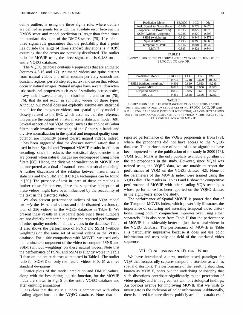
Table I show the performance of MOVIE in terms of theSpearman Rank Order Correlation Coefficient (SROCC), the

0 0.5 1 1.5 2 2.5 3 3.5 4−10

0

10

20

30

40

50

60

70

80

MOVIE score

DM

OS

(a)

0 0.5 1 1.5 2 2.5 3−10

0

10

20

30

40

50

60

70

80

MOVIE scoreD

MO

S(b)

Fig. 5. Scatter plot of the subjective DMOS scores against MOVIE scoreson the VQEG database. Each point on the plot represents one video in thedatabase. The best fitting logistic function used for non-linear regression isalso shown. (a) On all sequences in the VQEG database (b) After omittingthe animated videos.

Linear Correlation Coefficient (LCC) after non-linear regres-sion and the Outlier Ratio (OR). We used the same logisticfunction specified in [73] to fit the model predictions to thesubjective data. PSNR provides a baseline for comparisonof VQA models. Ten leading VQA models were tested bythe VQEG in its Phase 1 study including a model fromNTIA that was a precursor to VQM, as well as models fromNASA, Sarnoff Corporation, KDD and EPFL [73]. ProponentP8 (Swisscom) was the best performing model of these tenmodels tested by the VQEG [73]. SSIM (without weighting)refers to a frame-by-frame application of the SSIM indexthat was proposed for video in [4]. SSIM (weighting) refersto the model in [4] that incorporated rudimentary motioninformation as weights for different regions of the videosequence. Speed SSIM refers to the VQA algorithm in [5]that incorporates a model of human visual speed perceptionto design spatiotemporal weighting factors that are used toweight local SSIM indices in the pooling stage.

The Root Mean Squared Error (RMSE) between subjectivescores and MOVIE scores after non-linear regression on theentire VQEG database is 8.76. Outliers are defined by theVQEG as points for which the absolute error between theDMOS score and model prediction is larger than twice thestandard deviation of the DMOS score and the outlier ratiois defined as the ratio of the number of outlier videos tothe total number of videos [73]. A more standard way to

IEEE TRANSACTIONS ON IMAGE PROCESSING 13

define outliers is using the three sigma rule, where outliersare defined as points for which the absolute error between theDMOS score and model prediction is larger than three timesthe standard deviation of the DMOS scores [75]. Use of thethree sigma rule guarantees that the probability that a pointlies outside the range of three standard deviations is≤ 0.3%assuming that the errors are normally distributed. The outlierratio for MOVIE using the three sigma rule is0.488 on theentire VQEG database.

The VQEG database contains 4 sequences that are animated(sources 4,6,16 and 17). Animated videos are quite distinctfrom natural videos and often contain perfectly smooth andconstant regions, perfect step edges, text and so on that seldomoccur in natural images. Natural images have several character-istic statistical properties such as self-similarity across scales,heavy tailed wavelet marginal distributions and so on [70],[76], that do not occur in synthetic videos of these types.Although our model does not explicitly assume any statisticalmodel for the images or videos, our spatial quality model isclosely related to the IFC, which assumes that the referenceimages are the output of a natural scene statistical model [69].Several aspects of our VQA model such as the choice of Gaborfilters, scale invariant processing of the Gabor sub-bands anddivisive normalization in the spatial and temporal qualitycom-putation are implicitly geared toward natural videos. Indeed,it has been suggested that the divisive normalization that isused in both Spatial and Temporal MOVIE results in efficientencoding, since it reduces the statistical dependencies thatare present when natural images are decomposed using linearfilters [68]. Hence, the divisive normalization in MOVIE canbe interpreted as a dual of natural scene statistical modeling.A further discussion of the relation between natural scenestatistics and the SSIM and IFC IQA techniques can be foundin [69]. The presence of text in three of these animations isfurther cause for concern, since the subjective perceptionofthese videos might have been influenced by the readability ofthe text in the distorted video.

We also present performance indices of our VQA modelfor only the 16 natural videos and their distorted versions (atotal of 256 videos) in the VQEG database in Table II. Wepresent these results in a separate table since these numbersare not directly comparable against the reported performanceof other quality models on all the videos in the database. TableII also shows the performance of PSNR and SSIM (withoutweighting) on the same set of natural videos in the VQEGdatabase. For a fair comparison with MOVIE, we used onlythe luminance component of the video to compute PSNR andSSIM (without weighting) on these natural videos. Note thatthe performance of PSNR and SSIM is slightly worse in TableII than on the entire dataset as reported in Table I. The outlierratio for MOVIE on only the natural videos is 0.461 at threestandard deviations.

Scatter plots of the model prediction and DMOS values,along with the best fitting logistic function, for the MOVIEindex are shown in Fig. 5 on the entire VQEG database andafter omitting animations.

It is clear that the MOVIE index is competitive with otherleading algorithms on the VQEG database. Note that the

Prediction Model SROCC LCC ORPeak Signal to Noise Ratio 0.786 0.779 0.678Proponent P8 (Swisscom) 0.803 0.827 0.578SSIM (without weighting) 0.788 0.820 0.597

SSIM (weighting) 0.812 0.849 0.578Spatial MOVIE 0.793 0.796 0.666

Temporal MOVIE 0.816 0.801 0.647MOVIE 0.833 0.821 0.644

TABLE ICOMPARISON OF THE PERFORMANCE OFVQA ALGORITHMS USING

SROCC, LCCAND OR.

Prediction Model SROCC LCC OR RMSEPSNR 0.739 0.718 0.699 10.968

SSIM (without weighting) 0.802 0.810 0.633 9.245Spatial MOVIE 0.825 0.830 0.656 8.803

Temporal MOVIE 0.835 0.825 0.621 8.902MOVIE 0.860 0.858 0.656 8.093

TABLE IICOMPARISON OF THE PERFORMANCE OFVQA ALGORITHMS AFTER

OMITTING THE ANIMATION SEQUENCES USINGSROCC, LCC, ORAND

RMSE. PSNRAND SSIM (WITHOUT WEIGHTING) ARE COMPUTED USINGONLY THE LUMINANCE COMPONENT OF THE VIDEO IN THIS TABLE FOR A

FAIR COMPARISON WITHMOVIE.

reported performance of the VQEG proponents is from [73],where the proponents did not have access to the VQEGdatabase. The performance of some of these algorithms havebeen improved since the publication of the study in 2000 [73].VQM from NTIA is the only publicly available algorithm ofthe ten proponents in the study. However, since VQM wastrained using the VQEG data, we are unable to report theperformance of VQM on the VQEG dataset [42]. None ofthe parameters of the MOVIE index were trained using theVQEG data. The results in Tables I and II show the competitiveperformance of MOVIE with other leading VQA techniqueswhose performance has been reported on the VQEG datasetin the eight years since the study.

The performance of Spatial MOVIE is poorer than that ofthe Temporal MOVIE index, which powerfully illustrates theimportance of capturing and assessing temporal video distor-tions. Using both in conjunction improves over using eitherseparately. It is also seen from Table II that the performanceof MOVIE is considerably better on just the natural videos inthe VQEG database. The performance of MOVIE in TableI is particularly impressive because it does not use colorinformation and uses only one field of the interlaced videosequence.

VII. C ONCLUSIONS ANDFUTURE WORK

We have introduced a new, motion-based paradigm forVQA that successfully captures temporal distortions as well asspatial distortions. The performance of the resulting algorithm,known as MOVIE, bears out the underlying philosophy thatsuch distortions contribute significantly to the perception ofvideo quality, and is in agreement with physiological findings.An obvious avenue for improving MOVIE that we wish toinvestigate is the inclusion of color information. Additionally,there is a need for more diverse publicly available databases of

IEEE TRANSACTIONS ON IMAGE PROCESSING 14

reference videos, distorted videos, and statistically significantsubjective scores taken under carefully controlled measure-ment conditions to enable improved verification and testingof VQA algorithms. Such a database will be of great valueto the VQA research community, particularly in view of thefact that the videos from recent VQEG studies (including theVQEG FRTV-Phase 2 study and the Multimedia study) are notbeing made public [74]. Toward this end, we are creating sucha database of videos that will complement the existing LIVEImage Quality Database [77] and which seeks to improve theaccessibility and diversity of such data. The upcoming LIVEVideo Quality Database will be described in future reports.

Lastly, there naturally remains much open field for im-proving current competitive VQA algorithms. We believethat these will be improved by the development of bettermodels for naturalistic videos, for human image and motionprocessing, and by a better understanding of the nature ofdistortion perception. Important topics in these directionsinclude scalability of VQA, utilizing models of visual attentionand human eye movements in VQA [78], [79], [80], [6],exploration of advanced spatial and temporal pooling strategiesfor VQA [80], reduced reference VQA, and no reference VQA.However, in our view, the most important development in thefuture of both IQA and VQA is the deployment of the mostcompetitive algorithms for such diverse and important tasksas establishing video Quality of Service (QoS) in real-timeapplications; benchmarking the performance of competingimage and video processing algorithms, such as compression,restoration, and reconstruction; and optimizing algorithmsusing IQA and VQA indices to establish perceptual objectivefunctions [81]. This latter goal is the most ambitious owingto the likely formidable analytical challenges to be overcome,but may also prove to be the most significant.

APPENDIX

OPTICAL FLOW COMPUTATION V IA A NEW MULTI -SCALE

APPROACH

The Fleet and Jepson algorithm attempts to find constantphase contours of the outputs of a Gabor filterbank to estimatethe optical flow vectors [60]. Constant phase contours arecomputed by estimating the derivative of the phase of theGabor filter outputs, which in turn can be expressed as afunction of the derivative of the Gabor filter outputs [60]. Thealgorithm in [60] uses a 5-point central difference to performthe derivative computation. However, we chose to perform thederivative computation by convolving the video sequence withfilters that are derivatives of the Gabor kernels, denoted byh′

x(i), h′y(i), h

′t(i):

h′x(i) = h(i)

(−x

σ2+ jU0

)

(31)

Similar definitions apply for the derivatives alongy and tdirections. This filter computes the derivative of the Gaboroutputs more accurately and produced better optical flowestimates in our experiments.

Due to the aperture problem, each Gabor filter is only ableto signal the component of motion that is normal to its own

orientation. The Fleet and Jepson algorithm computes normalvelocity estimates at each pixel for each Gabor filter. Giventhe normal velocities from the different Gabor outputs, a linearvelocity model is fit to each local region using a least squarescriterion to obtain a 2D velocity estimate at each pixel of thevideo sequence. A residual error in the least squares solutionis also obtained at this stage. See [60], [82] for further details.

The original Fleet and Jepson algorithm uses just a singlescale of filters. We found that using a single scale of filterswas not sufficient, since optical flow was not computed in fastmoving regions of the several video sequences due to temporalaliasing [60], [57]. We hence used 3 scales of filters tocompute motion by extending the Fleet and Jepson algorithmto multiple scales. We compute a 2D velocity estimate at eachscale using the outputs of the Gabor filters at that scale only.It is important not to combine estimates across scales due totemporal aliasing [57], [60]. We also obtain an estimate of theresidual error in the least squares solution for each scale ofthe Gabor filterbank. The final flow vector at each pixel of thereference video is set to be the 2D velocity computed at thescale with the minimum residual error. Note that more complexsolutions such as coarse to fine warping methods have beenproposed in the literature to combine flow estimates acrossscales [83], [84], [85]. We chose this approach for simplicityand found that reasonable results were obtained.

The Fleet and Jepson algorithm does not produce flowestimates with 100% density, i.e. flow estimates are notcomputed at each and every pixel of the video sequence.Instead, optical flow is only computed at pixels where thereis sufficient information to do so. We set the optical flow tozero at all pixels where the flow was not computed.

REFERENCES

[1] Z. Wang and A. C. Bovik,Image Quality Assessment. New York:Morgan and Claypool Publishing Co., 2006.

[2] S. Winkler, Digital Video Quality. New York: Wiley and Sons, 2005.[3] C. J. van den Branden Lambrecht, D. M. Costantini, G. L. Sicuranza,

and M. Kunt, “Quality assessment of motion rendition in video coding,”IEEE Trans. Pattern Anal. Mach. Intell., vol. 9, no. 5, pp. 766–782, 1999.

[4] Z. Wang, L. Lu, and A. C. Bovik, “Video quality assessmentbased onstructural distortion measurement,”Signal Processing: Image Commu-nication, vol. 19, no. 2, pp. 121–132, Feb. 2004.

[5] Z. Wang and Q. Li, “Video quality assessment using a statistical modelof human visual speed perception.”Journal Optical Society America A:Optics Image Science Vision, vol. 24, no. 12, pp. B61–B69, Dec 2007.

[6] A. Ninassi, O. Le Meur, P. Le Callet, and D. Barba, “Considering tem-poral variations of spatial visual distortions in video quality assessment,”IEEE J. Sel. Topics Signal Process., vol. 3, no. 2, pp. 253–265, 2009.

[7] M. Barkowsky, J. Bialkowski, B. Eskofier, R. Bitto, and A.Kaup,“Temporal trajectory aware video quality measure,”IEEE J. Sel. TopicsSignal Process., vol. 3, no. 2, pp. 266–279, 2009.

[8] A. B. Watson and J. Ahumada, A. J., “Model of human visual-motionsensing,” Journal Optical Society America A: Optics Image ScienceVision, vol. 2, no. 2, pp. 322–342, 1985.

[9] K. Seshadrinathan and A. C. Bovik, “A structural similarity metric forvideo based on motion models,” inIEEE Intl. Conf. Acoustics, Speech,and Signal Processing, 2007.

[10] B. A. Wandell, Foundations of Vision. Sunderland, MA: SinauerAssociates Inc., 1995.

[11] L. Itti and C. Koch, “Computational modelling of visualattention,”Nature Reviews Neuroscience, vol. 2, no. 3, pp. 194–203, 2001.

[12] Z. Wang and A. Bovik, “A universal image quality index,”IEEE SignalProcess. Lett., vol. 9, no. 3, pp. 81–84, 2002.

[13] Z. Wang, A. C. Bovik, H. R. Sheikh, and E. P. Simoncelli, “Imagequality assessment: from error visibility to structural similarity,” IEEETrans. Image Process., vol. 13, no. 4, pp. 600–612, April 2004.

IEEE TRANSACTIONS ON IMAGE PROCESSING 15

[14] H. R. Sheikh and A. C. Bovik, “Image information and visual quality,”IEEE Trans. Image Process., vol. 15, no. 2, pp. 430–444, 2006.

[15] H. R. Sheikh, A. C. Bovik, and G. de Veciana, “An information fidelitycriterion for image quality assessment using natural scenestatistics,”IEEE Trans. Image Process., vol. 14, no. 12, pp. 2117–2128, 2005.

[16] H. R. Sheikh and A. C. Bovik, “An evaluation of recent full referenceimage quality assessment algorithms,”IEEE Trans. Image Process.,vol. 15, no. 11, pp. 3440–3451, November 2006.

[17] K. Seshadrinathan and A. C. Bovik, “An information theoretic videoquality metric based on motion models,” inThird Intl. Workshop VideoProcessing and Quality Metrics for Consumer Electronics, 2007.

[18] B. Girod, “What’s wrong with mean-squared error,” inDigital Imagesand Human Vision, A. B. Watson, Ed. The MIT Press, 1993, pp.207–220.

[19] K. Seshadrinathan and A. C. Bovik, “Video quality assessment,” inTheEssential Guide to Video Processing, A. C. Bovik, Ed. Elsevier, 2009.

[20] J. M. Libert, C. P. Fenimore, and P. Roitman, “Simulation of gradedvideo impairment by weighted summation: validation of the methodol-ogy,” Proc. SPIE, vol. 3845, no. 1, pp. 254–265, Nov. 1999.

[21] C. Lee and O. Kwon, “Objective measurements of video quality usingthe wavelet transform,”Optical Engineering, vol. 42, no. 1, pp. 265–272,Jan. 2003.

[22] C. Taylor and S. Dey, “Run-time allocation of buffer resources formaximizing video clip quality in a wireless last-hop system,” in Proc.IEEE Intl. Conf. Communications, 2004.

[23] J. Mannos and D. Sakrison, “The effects of a visual fidelity criterion ofthe encoding of images,”IEEE Trans. Inf. Theory, vol. 20, no. 4, pp.525–536, 1974.

[24] J. Lubin, “The use of psychophysical data and models in the analysisof display system performance,” inDigital Images and Human Vision,A. B. Watson, Ed. The MIT Press, 1993, pp. 163–178.

[25] P. C. Teo and D. J. Heeger, “Perceptual image distortion,” in Proc. IEEEIntl. Conf. Image Processing, 1994.

[26] S. Daly, “The visible difference predictor: An algorithm for the assess-ment of image fidelity,” inDigital Images and Human Vision, A. B.Watson, Ed. The MIT Press, 1993, pp. 176–206.

[27] D. M. Chandler, K. H. Lim, and S. S. Hemami, “Effects of spatialcorrelations and global precedence on the visual fidelity ofdistortedimages,”Proc. SPIE, vol. 6057, no. 1, p. 60570F, Feb 2006.

[28] K. Seshadrinathan, T. N. Pappas, R. J. Safranek, J. Chen, Z. Wang, H. R.Sheikh, and A. C. Bovik, “Image quality assessment,” inThe EssentialGuide to Image Processing, A. C. Bovik, Ed. Elsevier, 2008.

[29] G. E. Legge, “Sustained and transient mechanisms in human vision:Temporal and spatial properties,”Vision Research, vol. 18, no. 1, pp.69–81, 1978.

[30] J. J. Kulikowski and D. J. Tolhurst, “Psychophysical evidence forsustained and transient detectors in human vision.”Journal Physiology,vol. 232, no. 1, pp. 149–162, Jul 1973.

[31] C. J. van den Branden Lambrecht and O. Verscheure, “Perceptual qualitymeasure using a spatiotemporal model of the human visual system,”Proc. SPIE, vol. 2668, no. 1, pp. 450–461, Mar 1996.

[32] S. Winkler, “Perceptual distortion metric for digitalcolor video,” Proc.SPIE, vol. 3644, no. 1, pp. 175–184, May 1999.

[33] A. B. Watson, J. Hu, and J. F. McGowan III, “Digital videoqualitymetric based on human vision,”Journal Electronic Imaging, vol. 10,no. 1, pp. 20–29, Jan. 2001.

[34] M. Masry, S. S. Hemami, and Y. Sermadevi, “A scalable wavelet-basedvideo distortion metric and applications,”IEEE Trans. Circuits Syst.Video Technol., vol. 16, no. 2, pp. 260–273, 2006.

[35] J. A. Movshon and W. T. Newsome, “Visual Response Properties ofStriate Cortical Neurons Projecting to Area MT in Macaque Monkeys,”Journal Neuroscience, vol. 16, no. 23, pp. 7733–7741, 1996.

[36] R. T. Born and D. C. Bradley, “Structure and function of visual areaMT,” Annual Reviews Neuroscience, vol. 28, pp. 157–189, 2005.

[37] M. A. Smith, N. J. Majaj, and J. A. Movshon, “Dynamics of motionsignaling by neurons in macaque area MT,”Nature Neuroscience, vol. 8,no. 2, pp. 220–228, Feb. 2005.

[38] J. A. Perrone, “A visual motion sensor based on the properties of V1and MT neurons,”Vision Research, vol. 44, no. 15, pp. 1733–1755, Jul.2004.

[39] N. J. Priebe, S. G. Lisberger, and J. A. Movshon, “Tuningfor spatiotem-poral frequency and speed in directionally selective neurons of macaquestriate cortex.”Journal Neuroscience, vol. 26, no. 11, pp. 2941–2950,Mar 2006.

[40] J. Nachmias and R. V. Sansbury, “Grating contrast: Discrimination maybe better than detection,”Vision Research, vol. 14, no. 10, pp. 1039–1042, Oct. 1974.

[41] G. Legge and J. Foley, “Contrast masking in human vision,” JournalOptical Society America A: Optics Image Science Vision, vol. 70, no. 12,pp. 1458–1471, Dec. 1980.

[42] M. H. Pinson and S. Wolf, “A new standardized method for objectivelymeasuring video quality,”IEEE Trans. Broadcast., vol. 50, no. 3, pp.312–322, Sep. 2004.

[43] A. P. Hekstra, J. G. Beerends, D. Ledermann, F. E. de Caluwe, S. Kohler,R. H. Koenen, S. Rihs, M. Ehrsam, and D. Schlauss, “PVQM - A percep-tual video quality measure,”Signal Processing: Image Communication,vol. 17, pp. 781–798, 2002.

[44] International Telecommunications Union, “Objectiveperceptual multi-media video quality measurement in the presence of a full reference,”ITU-T Rec. J. 247, Tech. Rep., 2008.

[45] NTT. (2008) NTT News Release. [Online]. Available: http://www.ntt.co.jp/news/news08e/0808/080825a.html

[46] Opticom. [Online]. Available: http://www.opticom.de/technology/pevqvideo-quality-testing.html

[47] M. Malkowski and D. Claben, “Performance of video telephony servicesin UMTS using live measurements and network emulation,”WirelessPersonal Communications, vol. 1, pp. 19–32, 2008.

[48] M. Barkowsky, J. Bialkowski, R. Bitto, and A. Kaup, “Temporal regis-tration using 3D phase correlation and a maximum likelihoodapproachin the perceptual evaluation of video quality,” inIEEE WorkshopMultimedia Signal Processing, 2007.

[49] M. Yuen and H. R. Wu, “A survey of hybrid MC/DPCM/DCT videocoding distortions,”Signal Processing, vol. 70, no. 3, pp. 247–278, Nov.1998.

[50] K. Seshadrinathan and A. C. Bovik, “Motion-based perceptual qualityassessment of video,” inProc. SPIE - Human Vision and ElectronicImaging, 2009.

[51] J. A. Movshon, I. D. Thompson, and D. J. Tolhurst, “Spatial summationin the receptive fields of simple cells in the cat’s striate cortex.” JournalPhysiology, vol. 283, pp. 53–77, Oct 1978.

[52] J. G. Daugman, “Uncertainty relation for resolution inspace, spatialfrequency, and orientation optimized by two-dimensional visual corticalfilters,” Journal Optical Society America A: Optics Image Science Vision,vol. 2, no. 7, pp. 1160–1169, 1985.

[53] A. C. Bovik, M. Clark, and W. S. Geisler, “Multichannel texture analysisusing localized spatial filters,”IEEE Trans. Pattern Anal. Mach. Intell.,vol. 12, no. 1, pp. 55–73, Jan. 1990.

[54] D. J. Tolhurst and J. A. Movshon, “Spatial and temporal contrastsensitivity of striate cortical neurones,”Nature, vol. 257, no. 5528, pp.674–675, Oct. 1975.

[55] S. M. Friend and C. L. Baker, “Spatio-temporal frequency separabilityin area 18 neurons of the cat.”Vision Research, vol. 33, no. 13, pp.1765–1771, Sep 1993.

[56] M. C. Morrone, M. D. Stefano, and D. C. Burr, “Spatial andtemporalproperties of neurons of the lateral suprasylvian cortex ofthe cat.”Journal Neurophysiology, vol. 56, no. 4, pp. 969–986, Oct 1986.

[57] D. J. Heeger, “Optical flow using spatiotemporal filters,” Intl. JournalComputer Vision, vol. 1, no. 4, pp. 279–302, 1987.

[58] E. P. Simoncelli and D. J. Heeger, “A model of neuronal responses invisual area MT.”Vision Research, vol. 38, no. 5, pp. 743–761, Mar1998.

[59] E. H. Adelson and J. R. Bergen, “Spatiotemporal energy models forthe perception of motion.”Journal Optical Society America A: OpticsImage Science Vision, vol. 2, no. 2, pp. 284–299, Feb 1985.

[60] D. Fleet and A. Jepson, “Computation of component imagevelocityfrom local phase information,”Intl. Journal Computer Vision, vol. 5,no. 1, pp. 77–104, 1990.

[61] H. R. Sheikh and A. C. Bovik, “A visual information fidelity approachto video quality assessment,” inFirst Intl. workshop video processingand quality metrics for consumer electronics, 2005.

[62] R. Fox, “Visual masking,” inHandbook of Sensory Physiology. VIII.Perception, R. Held, H. W. Leibowitz, and H. L. Teuber, Eds. Springer-Verlag, 1978.

[63] J. Foley, “Human luminance pattern-vision mechanisms: masking ex-periments require a new model,”Journal Optical Society America A:Optics Image Science Vision, vol. 11, no. 6, pp. 1710–1719, Jun. 1994.

[64] A. Watson and J. Solomon, “Model of visual contrast gaincontrol andpattern masking,”Journal Optical Society America A: Optics ImageScience Vision, vol. 14, no. 9, pp. 2379–2391, Sep. 1997.

[65] D. J. Heeger, “Normalization of cell responses in cat striate cortex.”Visual Neuroscience, vol. 9, no. 2, pp. 181–197, Aug 1992.

[66] D. G. Albrecht and W. S. Geisler, “Motion selectivity and the contrast-response function of simple cells in the visual cortex.”Visual Neuro-science, vol. 7, no. 6, pp. 531–546, Dec 1991.

IEEE TRANSACTIONS ON IMAGE PROCESSING 16

[67] W. S. Geisler and D. G. Albrecht, “Cortical neurons: isolation of contrastgain control.”Vision Research, vol. 32, no. 8, pp. 1409–1410, Aug 1992.

[68] O. Schwartz and E. P. Simoncelli, “Natural signal statistics and sensorygain control.” Nature Neuroscience, vol. 4, no. 8, pp. 819–825, Aug2001.

[69] K. Seshadrinathan and A. C. Bovik, “Unifying analysis of full referenceimage quality assessment,” inIEEE Intl. Conf. Image Processing, 2008.

[70] D. J. Field, “Relations between the statistics of natural images and theresponse properties of cortical cells.”Journal Optical Society AmericaA: Optics Image Science Vision, vol. 4, no. 12, pp. 2379–2394, Dec1987.

[71] J. A. Perrone and A. Thiele, “Speed skills: measuring the visual speedanalyzing properties of primate MT neurons,”Nature Neuroscience,vol. 4, no. 5, pp. 526–532, May 2001.

[72] N. C. Rust, V. Mante, E. P. Simoncelli, and J. A. Movshon,“How MTcells analyze the motion of visual patterns.”Nature Neuroscience, vol. 9,no. 11, pp. 1421–1431, Nov 2006.

[73] (2000) Final report from the video quality experts group on the validationof objective quality metrics for video quality assessment.[Online].Available: http://www.its.bldrdoc.gov/vqeg/projects/frtv phaseI

[74] A. Webster, “Progress and future plans for VQEG,” inETSISTQ Workshop Multimedia Quality of Service, 2008. [Online].Available: http://portal.etsi.org/docbox/Workshop/2008/2008 06STQWORKSHOP/VQEGArthurWebster.pdf

[75] S. H. Dai and M. O. Wang,Reliability analysis in engineering applica-tions. Van Nostrand Reinhold, 1993.

[76] E. P. Simoncelli, “Statistical modeling of photographic images,” inHandbook of Image and Video Processing, 2nd ed., A. C. Bovik, Ed.Academic Press, 2005.

[77] (2003) LIVE image quality assessment database. [Online]. Available:http://live.ece.utexas.edu/research/quality/subjective.htm

[78] A. K. Moorthy and A. C. Bovik, “Perceptually significantspatial poolingstrategies for image quality assessment,” inProc. SPIE - Human Visionand Electronic Imaging, 2009.

[79] U. Rajashekar, I. van der Linde, A. C. Bovik, and L. K. Cormack,“GAFFE: A gaze-attentive fixation finding engine,”IEEE Trans. ImageProcess., vol. 17, no. 4, pp. 564–573, 2008.

[80] A. K. Moorthy and A. C. Bovik, “Visual importance pooling for imagequality assessment,”IEEE J. Sel. Topics Signal Process., vol. 3, no. 2,pp. 193–201, 2009.

[81] S. S. Channappayya, A. C. Bovik, C. Caramanis, and R. W. Heath,Jr., “Design of linear equalizers optimized for the structural similarityindex,” IEEE Trans. Image Process., vol. 17, no. 6, pp. 857–872, 2008.

[82] J. L. Barron, D. J. Fleet, and S. S. Beauchemin, “Performance of opticalflow techniques,”Intl. Journal Computer Vision, vol. 12, no. 1, pp. 43–77, Feb. 1994.

[83] E. P. Simoncelli, “Distributed analysis and representation of visualmotion,” Ph.D. dissertation, MIT, 1993.

[84] P. Anandan, “A computational framework and an algorithm for themeasurement of visual motion,”Intl. Journal Computer Vision, vol. 2,no. 3, pp. 283–310, Jan. 1989.

[85] B. D. Lucas and T. Kanade, “An iterative image registration techniquewith an application to stereo vision,” inProc. Intl. Joint Conf. ArtificialIntelligence, Vancouver, Canada, 1981.

Kalpana Seshadrinathan Kalpana Seshadrinathanreceived the B.Tech. degree from the University ofKerala, India in 2002 and the M.S. and Ph.D. degreesin Electrical Engineering from the University ofTexas at Austin, in 2004 and 2008, respectively. Sheis currently a System Engineer with Intel Corpora-tion in Phoenix, AZ. Her research interests includeimage and video quality assessment, computationalaspects of human vision, motion estimation andits applications and statistical modeling of imagesand video. She is a recipient of the 2003 Texas

Telecommunications Engineering Consortium Graduate Fellowship and the2007 Graduate Student Professional Development Award fromthe Universityof Texas at Austin. She was Assistant Director of the Laboratory for Imageand Video Engineering (LIVE) at the University of Texas at Austin from2005-2008. She is a member of the IEEE.

Alan Conrad Bovik Alan Conrad Bovik is theCurry/Cullen Trust Endowed Chair Professor at TheUniversity of Texas at Austin, where he is theDirector of the Laboratory for Image and VideoEngineering (LIVE). He is a faculty member in theDepartment of Electrical and Computer Engineering,the Department of Biomedical Engineering, and theInstitute for Neuroscience. His research interestsinclude image and video processing, computationalvision, and visual perception. He has published over500 technical articles in these areas and holds two

U.S. patents. He is the author ofThe Handbook of Image and Video Processing(Academic Press, 2005),Modern Image Quality Assessment(Morgan & Clay-pool, 2006), and two new books,The Essential Guide to Image ProcessingandThe Essential Guide to Video Processing(Academic Press).

Dr. Bovik has received a number of major awards from the IEEE SignalProcessing Society, including: the Education Award (2008); the TechnicalAchievement Award (2005), the Distinguished Lecturer Award (2000); and theMeritorious Service Award (1998). He is also a recipient of the Hocott Awardfor Distinguished Engineering Research at the University of Texas at Austin;received the Distinguished Alumni Award from the University of Illinoisat Champaign-Urbana (2008), the IEEE Third Millennium Medal (2000)and two journal paper awards from the international PatternRecognitionSociety (1988 and 1993). He is a Fellow of the IEEE, a Fellow oftheOptical Society of America, and a Fellow of the Society of Photo-Optical andInstrumentation Engineers. He has been involved in numerous professionalsociety activities, including: Board of Governors, IEEE Signal ProcessingSociety, 1996-1998; Editor-in-Chief,IEEE Transactions on Image Processing,1996-2002; Editorial Board,The Proceedings of the IEEE, 1998-2004; SeriesEditor for Image, Video, and Multimedia Processing, Morganand ClaypoolPublishing Company, 2003-present; and Founding General Chairman, FirstIEEE International Conference on Image Processing, held in Austin, Texas,in November, 1994.

Dr. Bovik is a registered Professional Engineer in the Stateof Texas andis a frequent consultant to legal, industrial and academic institutions.