Embed Size (px)
Citation preview
IEEE TRANSACTIONS ON FUZZY SYSTEMS, VOL. 25, NO. 5, OCTOBER 2017 1293
Hybrid Robust Boundary and Fuzzy Control forDisturbance Attenuation of Nonlinear Coupled
ODE-Beam Systems With Application to aFlexible Spacecraft
Shuang Feng and Huai-Ning Wu
Abstract—This paper introduces a hybrid robust boundaryand fuzzy control design for disturbance attenuation of a classof coupled systems described by nonlinear ordinary differentialequations (ODEs) and two nonlinear beam equations. Initially, aTakagi–Sugeno (T–S) model is employed to exactly represent thenonlinear ODE subsystem. Then, a fuzzy controller is designed forthe ODE subsystem based on the T–S fuzzy model, and a robustboundary controller via beam boundary measurements is proposedfor the nonlinear beam subsystem. Such a hybrid robust bound-ary and fuzzy controller is developed in terms of a set of space-dependent bilinear matrix inequalities (BMIs) by Lyapunov’s di-rect method, which can exponentially stabilize the coupled systemin the absence of disturbances and achieve an prescribed H∞performance of disturbance attenuation in the presence of distur-bances. Furthermore, in order to make the level of disturbance at-tenuation as small as possible, a suboptimalH∞ control problem isformulated as a BMI optimization problem. A two-step procedureis subsequently presented to solve this BMI optimization problemby the existing linear matrix inequality optimization techniques.Finally, the proposed control method is applied to the control of aflexible spacecraft to illustrate its effectiveness.
Index Terms—Coupled ordinary differential equation (ODE)-beam systems, fuzzy control, robust boundary control,H∞ control,exponential stability.
I. INTRODUCTION
THE phenomenon of structural vibration widely existsin flexible mechanical systems, such as a solar electric
propulsion spacecraft [1] and flexible risers with vessel dynam-ics [2]. Undesirable vibration may limit the accuracy of sensitiveinstruments or even cause significant errors when high-precisionpositioning is required [3]. Thus, vibration suppression is anecessity for fast maneuvers of such flexible mechanicalsystems, which can be described by a class of beam equations
Manuscript received June 21, 2016; accepted August 8, 2016. Date of publi-cation September 21, 2016; date of current version October 4, 2017. This workwas supported in part by the National Natural Science Foundations of Chinaunder Grant 61625302, Grant 61473011, and Grant 61421063, and in part by theAcademic Excellence Foundation of BUAA for PhD Students. (Correspondingauthor: Huai-Ning Wu.)
The authors are with the Science and Technology on Aircraft Control Labo-ratory, School of Automation Science and Electrical Engineering, Beihang Uni-versity, Beijing 100191, China (e-mail: [email protected]; [email protected]).
Color versions of one or more of the figures in this paper are available onlineat http://ieeexplore.ieee.org.
Digital Object Identifier 10.1109/TFUZZ.2016.2612264
coupled with ordinary differential equations (ODEs). However,the analysis and control synthesis for these systems are morechallenging because of their complex form and infinite-dimensional nature. One of the control strategies is thediscretization of the beam equation into the finite-dimensionalODEs by Galerkin’s method or the assumed modes method, andthen, many conventional control schemes for ODE systems canbe directly applied to such truncated model [4]–[7]. Neverthe-less, the control and observation spillover problem may occurdue to ignored higher frequency modes [4]. To overcome thisshortcoming, a great deal of progress has been made in studyingcontrol methods based on the original coupled ODE-beammodel. For example, Morgul [8] studied the orientation andstabilization problem of a flexible beam attached to a rigidbody; the dynamic boundary control method was given for anonhomogeneous rotating body-beam in [9]; Zhao and Weissanalyzed the properties of the well posedness, regularity, andexact controllability for a linear Euler–Bernoulli beam equationcoupled with an ODE model [10], and then, developed acollocated static output feedback controller for a wind turbinetower described by a coupled ODE-beam model in [11]; Chenet al. [12] addressed the stabilization problem of a rotatingdisk–beam–mass system. However, it is worth pointing out thatthe all control schemes in [8], [9], [11], and [12] are based onthe abstract semigroup theory, which limits the realization ofthese methods in practical engineering applications.
Recently, Lyapunov’s direct method has been employed forthe control design of coupled ODE-beam systems, which iseasy to use in practice. For instance, a robust adaptive boundarycontroller was developed for a flexible marine riser with vesseldynamics in [2]; the modeling and vibration control problemwas addressed for a satellite with flexible solar panels in [13];a static output feedback control design via PDE boundary andODE measurements was proposed for a class of linear cascadedODE-beam systems in [14]; in [15], a feedback control designvia ODE state feedback and PDE boundary output feedbackwas presented to suppress the vibrations for an air-breathinghypersonic vehicle represented by a nonlinear coupled ODE-beam model, where the nonlinear ODE model is linearizedon a trimmed equilibrium point by using a small perturbationmethod. It should be pointed out that the control methods in[2], [13]–[15] are only available for the linear beam equation
1063-6706 © 2016 IEEE. Personal use is permitted, but republication/redistribution requires IEEE permission.See http://www.ieee.org/publications standards/publications/rights/index.html for more information.
1294 IEEE TRANSACTIONS ON FUZZY SYSTEMS, VOL. 25, NO. 5, OCTOBER 2017
coupled with a linear or nonlinear ODE model. Therefore, de-spite these efforts, the modeling and control for nonlinear beamequations coupled with the nonlinear ODE model have still beenone of most challenging areas for system and control theory.
On the other hand, many flexible mechanical systems, suchas flexible spacecraft [16], have strong nonlinear characteristics,which usually make the analysis and control synthesis more dif-ficult. As is well known, the Takagi–Sugeno (T–S) fuzzy model[17] is one of most efficient techniques to describe complexnonlinear systems, and the T–S fuzzy-model-based control hasattracted considerable attention since it combines the merits ofboth the fuzzy logic theory and the linear system theory [18]–[20]. The fuzzy logic theory enables us to decompose the taskof modeling and control for a complex nonlinear system into agroup of easier local tasks by utilizing its qualitative linguisticinformation. And then, the overall model and control designis constructed by combining all the local tasks through fuzzymembership functions. Hence, based on the T–S fuzzy model,the fruitful linear system theory [21], [22] can be applied tothe analysis and synthesis of nonlinear systems. Recently, theresults on this fuzzy control technique have been extended frompure nonlinear ODEs [17]–[20] to partial differential equations(PDEs) via early lumping [23], [24] or late lumping [25], [26].More recently, this fuzzy control technique has been further ap-plied to nonlinear coupled PDE–ODE systems. For example,in [27], the problem of fuzzy boundary control design was ad-dressed for a nonlinear ODE model cascaded by a linear hyper-bolic PDE. In fact, the control-oriented model for many practicalapplications is of much more complexity, where the PDE hasalso strong nonlinearities and the coupling interactions exist inboth the ODE and PDE. For instance, a flexible spacecraft wasmodeled in [16] by nonlinear ODEs coupled with two nonlinearbeam equations, and a proportional control design was pre-sented for this complex nonlinear coupled system. Moreover, inpractice, it is usually desirable for control engineers to designa controller that not only stabilizes such nonlinear coupled sys-tem, but also provides a satisfactory performance of disturbanceattenuation. Motivated by the above facts, in this paper, an H∞hybrid fuzzy and robust boundary control design will be devel-oped for nonlinear coupled ODE-beam systems with externaldisturbances.
In this study, we will address the hybrid robust boundary andfuzzy control problem for a class of coupled systems consistingof an n-dimensional nonlinear ODE model and two nonlinearbeam equations. The T–S fuzzy model is initially employedto represent the nonlinear ODE subsystem. Subsequently, afuzzy controller is constructed for this subsystem based on thefuzzy model and the parallel distributed compensation (PDC)scheme [18], and a robust boundary controller is adopted for thebeam equations by only using beam boundary measurements.With Lyapunov’s direct method, the hybrid robust boundaryand fuzzy control design is then developed in terms of a setof space-dependent bilinear matrix inequalities (BMIs), whichcan exponentially stabilize the coupled system in the absenceof disturbances and achieve a prescribed H∞ performance ofdisturbance attenuation. Furthermore, a suboptimal H∞ controlproblem is formulated as a BMI optimization problem to makethe attenuation level as small as possible. And then, a two-step
procedure is proposed to solve this BMI optimization problemby the existing linear matrix inequality (LMI) optimization tech-niques [21], [28]. Finally, a simulation study on the control ofa flexible spacecraft is given to show the effectiveness of theproposed design method.
The rest of this paper is organized as follows. Section II givesthe preliminaries and problem formulation. Section III presentsthe H∞ hybrid fuzzy and robust boundary control method. InSection IV, simulation results on a flexible spacecraft illustratethe effectiveness of the proposed design method. Finally, someconclusions are drawn in Section V.
Notations: R, Rn , Rn×m denote the set of real numbers,the n-dimensional Euclidean space, and the set of all realn × m matrices, respectively. ‖ · ‖ is the Euclidean norm forvectors. For a symmetric matrix M , M > (<, ≤) 0 meansthat it is positive definite (negative definite, negative semidef-inite, respectively). The space-varying symmetric matrix func-tion Q(η), η ∈ [0, L] is positive definite (negative definite),if Q(η) > (<) 0 for all η ∈ [0, L]. λmax(·) and λmin(·) standfor the maximum and minimum eigenvalues of a square ma-trix, respectively. The superscript T is used for the transposeof a matrix or a vector. For any integer l ≥ 0, W l, 2(0, L)is a Sobolev space of absolutely continuous vector functions:ω(η) : [0, L] → R2 with square integrable derivatives ω(l)(η)of the order l and with the inner product 〈ω1(·), ω2(·)〉W l , 2
Δ=∫ L
0
∑li=0 ω
(i)1 (·)T ω
(i)2 (·)dη and the inner product induced norm
‖ω1(·)‖2W l , 2
Δ=∫ L
0
∑li=0 ‖ω(i)
1 (η)‖2dη where ω1(·), ω2(·) ∈
W l, 2(0, L). This space is also a Hilbert space with the corre-sponding inner product and denoted by Hl(0, L). The symbol∗ is used as an ellipsis for terms in matrix expressions that areinduced by symmetry, for example
[S + [M + ∗] ∗
X Y
]Δ=[S + [M +MT ] XT
X Y
]
.
II. PRELIMINARIES AND PROBLEM FORMULATION
Consider a class of nonlinear coupled ODE-beam systemsdescribed by the following n-dimensional nonlinear ODE withthe beam equations:
x(t) = f 1(x(t)) +∫ L
0(R + η)f 2(x(t))ξt(η, t)dη
+ g(x(t))u(t) + d1(t)
(1)
EIξηηηη (η, t) + ρξtt(η, t)
+f 3(x, ξ(η, t), ξt(η, t))+f 4(x, η)+d2(η, t)=0 (2)
subject to the boundary conditions
ξ(0, t) = ξη (0, t) = 0, EIξηη (L, t) = 0,
EIξηηη (L, t) = v(t) (3)
and the initial conditions
x(0) = x0 , ξ(η, 0) = ξ0(η), ξt(η, 0) = ξt,0(η) (4)
where x(t) ∈ Rn is the state of the ODE system (1); u(t) ∈ Rp
is the manipulated input; ξ(η, t) ∈ R2 is the transverse displace-
FENG AND WU: HYBRID ROBUST BOUNDARY AND FUZZY CONTROL FOR DISTURBANCE ATTENUATION 1295
ment of the beam (2); the subscripts η and t stand for the partialderivatives with respect to η and t, respectively, η ∈ [0, L] ⊂ Rrepresents the spatial position; v(t) ∈ R2 is the boundary inputof the beam; d1(t) and d2(η, t) are the bounded exogenousdisturbances; f 1(x(t)), f 2(x(t)), and g(x(t)) are locally Lip-schitz continuous nonlinear functions satisfying f 1(0) = 0 andf 2(0) = 0; f 3(x, ξ(η, t), ξt(η, t)) and f 4(x, η) are contin-uous functions satisfying f 3(0, 0, 0) = 0 and f 4(0, η) = 0;EI is the flexural rigidity of the beam; ρ is the mass densityof the beam; R is a positive number; L > 0 is the length of thebeam; x0 , ξ0(η) , and ξt,0(η) are initial conditions.
Remark 1: The coupled ODE-beam model in (1)–(4) candescribe the dynamics of flexible mechanical systems. For ex-ample, in the case of a flexible spacecraft, consisting of a rigidbody and flexible appendage, such as a long beam, solar panel,and antenna, x(t) can denote the angular velocity of the rigidbody and ξ(η, t) describes the transverse vibrations of the flex-ible part. The integral term of (1) represents the contribution ofthe beam vibrations to the total angular momentum of the rigidbody, whereas the influence of the rigid body rotation is de-scribed as the nonlinear functions f 3(x, ξ, ξt) and f 4(x, η)in (2) on the beam vibrations.
First, denote H(0, L) Δ= H2L (0, L) × L2(0, L) with the
norm
‖ς(·, t)‖2H
=∫ L
0(EIξT
ηη (η, t)ξηη (η, t) + ρξTt (η, t)ξt(η, t))dη
where ς(η, t) Δ= [ξT (η, t) ξTt (η, t) ]T ∈ H(0, L), η ∈ [0, L]
⊂ R, t ≥ 0, and
H2L (0, L) Δ= {ξ|ξ ∈ H2(0, L), ξ(0, t) = ξη (0, t) = 0},
L2(0, L) Δ=
⎧⎨
⎩ξt : [0, L] → R2 |
√∫ L
0ξT
t ξtdη < ∞⎫⎬
⎭.
H(0, L) is then a Hilbert space [29], [30] and so is HΔ= Rn ×
H(0, L) with the norm
‖ϑ(·, t)‖2H
Δ=12xT Px+
12
∫ L
0(EIξT
ηηξηη + ρξTt ξt)dη
(5)
where ϑ(η, t) Δ= [xT (η, t) ςT (η, t) ]T ∈ H.Definition 1 [14]: The disturbance-free unforced nonlinear
coupled system (1)–(4) [i.e., u(t) ≡ 0 and v(t) ≡ 0] is saidto be exponentially stable, if there exist positive constants δ,ε, and σ such that for any ‖ϑ(·, 0)‖H ≤ δ where ϑ(·, 0) =[xT
0 ξT0 ( · ) ξT
t,0( · ) ]T , the solution ϑ of the system (1)–(4)satisfies ‖ϑ(·, t)‖2
H ≤ ε‖ϑ(·, 0)‖2H exp(−σt).
Assumption 1: There exist positive constants k1 , k2 , k3 , andk4 such that
‖f 3(x, ξ, ξt)‖22 ≤ k1‖x‖2 + k2 ‖ξ‖2
2 + k3 ‖ξt‖22 (6)
‖f 4(x, η)‖22 ≤ k4‖x‖2 . (7)
As is known, with the sector nonlinearity approach [18], acomplex nonlinear system is exactly represented by a T–S fuzzy
model. This fuzzy model is described by fuzzy IF–THEN rulesand will be then exploited to handle the control design problemof the nonlinear coupled system (1) and (2). The ith rule ofthis fuzzy model for the nonlinear ODE subsystem (1) is of thefollowing form:
Plant Rule i :IF θ1(t) is Mi1 and . . . and θl(t) is Mil
THEN
x = A1, ix+∫ L
0(R + η)A2, iξtdη +Biu+ d1 (8)
where A1, i , A2, i , Bi , and i ∈ SΔ= {1, . . . , r} are known real
matrices with appropriate dimensions, r is the number of if–thenrules, Mij , j = 1, . . . , l are fuzzy sets, θ1 ∼ θl are premise vari-ables which are assumed to be functions of ODE state variables.
The overall dynamics of the fuzzy system is inferred as fol-lows:
x = A1(θ)x+∫ L
0(R + η)A2(θ)ξtdη +B(θ)u+ d1 (9)
where θΔ= [ θ1 · · · θl ]T , and
A1(θ) =r∑
i=1
hi(θ)A1, i , A2(θ) =r∑
i=1
hi(θ)A2, i ,
B(θ) =r∑
i=1
hi(θ)Bi , hi(θ) = μi(θ)/r∑
i=1
μi(θ),
μi(θ) =l∏
j=1
Mij (θj )
in which Mij (θj ) is the grade of membership of θj in Mij .Assume that μi(θ) ≥ 0, i ∈ S, and
∑ri=1 μi(θ) > 0 for all t.
Then, we have hi(θ) ≥ 0 and∑r
i=1 hi(θ) = 1.Based on the fuzzy model (8) and the PDC scheme [18], the
following fuzzy controller is considered for the ODE subsystem(8):
Control Rule j :IF θ1(t) is Mj1 and . . . and θl(t) is Mjl
THEN u(t) = Ks, jx(t), j ∈ Swhere Ks, j ∈ Rp×n , j ∈ S are feedback gain matrices to bedetermined. The overall fuzzy controller of the ODE subsystemis represented by
u(t) = Ks(θ)x(t) (10)
whereKs(θ)Δ=∑r
j=1 hj (θ)Ks, jx(t).Remark 2: In the study, we assume that all state variables
of nonlinear ODE subsystem (1) are available. Thus, so are allpremise variables because they are functions of the ODE statevariables. Then, the fuzzy controller (10) can be constructedwith the available information. When the ODE state variables arenot fully available, a state observer is necessary to estimate theODE state variables and reconstruct the premise variables fromthe measurable output information with measurement error. Inthis case, the control problem becomes more challenging whichis left for future research. Moreover, the measurement noise isalso not considered in this study, and it is very meaningful to take
1296 IEEE TRANSACTIONS ON FUZZY SYSTEMS, VOL. 25, NO. 5, OCTOBER 2017
the measurement noise into account for the stability analysis andcontrol synthesis in practice.
On the other hand, we consider a boundary controller viaboundary measurements for the beam subsystem (2) and (3) asfollows:
v(t) = Kbψ(t) (11)
whereKb ∈ R2×4 , ψ(t) Δ= [ξTt (L, t) ξT
η (L, t)]T ∈ R4 .Remark 3: In this paper, a hybrid robust boundary and fuzzy
controller of the forms (10) and (11) is designed to stabilize thenonlinear coupled ODE-beam system in (1)–(4). More specifi-cally, the fuzzy control law in (10) is applied to the control ofthe nonlinear ODE subsystem, and the robust boundary controllaw in (11) is used to suppress the vibrations by only usingthe boundary measurements of the beam, where the velocityξt(L, t) and angle ξη (L, t) at the free end of the beam (2)and (3) can be sensed by the velocity sensor and inclinometer,respectively.
Then, substituting (10) and (11) into (9) and (3), respectively,yields the following closed-loop coupled system:
x = Ac(θ)x+∫ L
0(R + η)A2(θ)ξtdη + d1 , x(0) = x0
(12)⎧⎪⎪⎪⎨
⎪⎪⎪⎩
EIξηηηη + ρξtt + f 3(x, ξ, ξt) + f 4(x, η) + d2 = 0ξ(0, t) = ξη (0, t) = 0,
EIξηη (L, t) = 0, EIξηηη (L, t) = Kbψ
ξ(η, 0) = ξ0(η), ξt(η, 0) = ξt,0(η)
(13)
whereAc(θ)Δ= A1(θ) +B(θ)Ks(θ).
In practical applications, it is usually desirable to design a con-trol system that is not only stable but also guarantees an adequatelevel of performance. For the external disturbances d1(t) andd2(η, t), the following H∞ control performance will be con-sidered under zero initial conditions (i.e., x0 = 0, ξ0(η) = 0,ξt,0(η) = 0):
∫ tf
0
∫ L
0(xT (η, t)Qx(η, t) + uT (t)Ru(t))dηdt
≤ γ2∫ tf
0
∫ L
0d
T(η, t)d(η, t)dηdt (14)
where x(η, t) Δ= [xT (t) ξT (η, t) ]T , u(t) Δ= [uT (t) vT (t) ]T ,
d(η, t) Δ= [dT1 (t) dT
2 (η, t) ]T , tf is the specified terminal-timeof control, γ is a prescribed level of disturbance attenu-ation level, Q = CTC > 0 ∈ R(n+2)×(n+2) , R = DTD ≥0 ∈ R(p+2)×(p+2) are given weighting matrices in which C
Δ=diag{ C1 , C2}, D
Δ= diag{D1 , D2}, C1 ∈ Rn×n , C2 ∈R2×2 ,D1 ∈ Rp×p , andD2 ∈ R2×2 .
Therefore, the control design problem under considerationis to find a fuzzy control law of the form (10) and a robustboundary control law of the form (11) for the nonlinear coupledODE-beam system (1)–(4), such that the closed-loop coupledsystem (12) and (13) is exponentially stable in the absence ofd(η, t), and the H∞ control performance of (14) is satisfied in
the presence of d(η, t). For convenience, such a controller iscalled an H∞ hybrid robust boundary and fuzzy controller. Fur-thermore, a suboptimal H∞ control problem is also addressedin the sense of minimizing the disturbance attenuation level γ.
Remark 4: In this study, the term “hybrid” means that thecontrol scheme includes two separate control laws: a fuzzy con-trol law u(t) and a robust boundary control law v(t), whereu(t) is acting on the nonlinear ODE subsystem (1) via ODEstate feedback and v(t) is applied to the beam (2) and (3) forthe vibration suppression with beam boundary measurements.
The following lemma is useful in the sequel.Lemma 1 [31]: Let ξ(·, t) ∈ L2(0, L) be an absolutely
continuous vector function with square integrable derivativeξη (·, t) and ξ(0, t) = 0. Then, for any matrixM > 0 ∈ R2×2 ,the following inequality holds:∫ L
0ξT (η, t)Mξ(η, t)dη ≤ 4L2π−2
∫ L
0ξT
η (η, t)Mξη (η, t)dη.
III. MAIN RESULTS
In this section, we will first present a space-dependent BMI-based design method for deriving the H∞ hybrid robust bound-ary and fuzzy controller of the forms (10) and (11). Then, tomake the attenuation level as small as possible, a suboptimalH∞ control problem is formulated as a BMI optimization prob-lem, which can be solved by a two-step design procedure.
Consider the following Lyapunov candidate for the closed-loop system (12) and (13):
V (t) = V1(x(t)) + V2(ζ(η, t)) + V3(ξηη (η, t)) (15)
where
V1(x) = xT Px,
V2(ζ) =∫ L
0ζT (η, t)Q(η)ζ(η, t)dη,
V3(ξηη ) =∫ L
0EIξT
ηηQ11ξηη dη
in which ζ(η, t) Δ= [ξTt ξT
η ]T , P > 0 ∈ Rn×n , Q(η) Δ=[ ρQ1 1ρηQ1 2
∗Q2 2
] > 0, Q11 , Q22 , Q12 > 0 ∈ R2×2 . Subsequently,from (5) and (15), we have
p1 ‖ϑ(·, t)‖2H ≤ V ≤ p2(‖ϑ(·, t)‖2
H +∫ L
0ρξT
η ξη dη) (16)
where
p1Δ= 2min{1, min
η∈[0, L ]ρ−1λmin(Q(η)), λmin(Q11)},
p2Δ= 2max {1, max
η∈[0, L ]ρ−1λmax(Q(η)), λmax(Q11)}.
Considering ξη (0, t) = 0, and then, using Lemma 1, we get∫ L
0ρξT
η ξη dη ≤ 4L2π−2ρEI−1∫ L
0EIξT
ηηξηη dη. (17)
It is clear from (16) and (17) that
p1 ‖ϑ(·, t)‖2H ≤ V ≤ p3 ‖ϑ(·, t)‖2
H (18)

FENG AND WU: HYBRID ROBUST BOUNDARY AND FUZZY CONTROL FOR DISTURBANCE ATTENUATION 1297
where p3Δ= p2(1 + 8L2π−2ρEI−1). Then, it is obvious from
(18) that the Lyapunov candidate (15) is equivalent to‖ϑ(·, t)‖2
H in H, which will be employed for the stability anal-ysis of the closed-loop coupled ODE-beam system (1) and (4).
Next, calculating the derivative of V given by (15) along thetrajectories of the closed-loop system (12) and (13), gives that
V = V1 + V2 + V3 (19)
where
V1 = 2xT P
[
Ac(θ)x+∫ L
0(R + η)A2(θ)ξt(η, t)dη + d1
]
(20)
V2 = 2∫ L
0ρξT
t Q11ξttdη + 2∫ L
0ρηξT
t Q12ξηtdη
+ 2∫ L
0ρηξT
ttQ12ξη dη + 2∫ L
0ξT
η Q22ξηtdη (21)
V3 = 2∫ L
0EIξT
ηηQ11ξηηtdη. (22)
Notice that there are four integral terms in (21), and theycan be calculated separately by considering (13) and using theintegration by parts formula as follows:
2∫ L
0ρξT
t Q11ξttdη
=−2∫ L
0ξT
t Q11 [EIξηηηη +f 3(x, ξ, ξt)+f 4(x, η) + d2 ]dη
= −2ξTt (L, t)Q11Kbψ(t)
− 2EI
∫ L
0ξT
tηηQ11ξηη dη − 2∫ L
0ξT
t Q11f 3(x, ξ, ξt)dη
− 2∫ L
0ξT
t Q11f 4(x, η)dη − 2∫ L
0ξT
t Q11d2dη (23)
2∫ L
0ρηξT
t Q12ξηtdη = 2ρLξTt (L, t)Q12ξt(L, t)
− 2∫ L
0ρηξT
ηtQ12ξtdη − 2∫ L
0ρξT
t Q12ξtdη (24)
2∫ L
0ρηξT
ttQ12ξη dη
=−2∫ L
0ηξT
η Q12 [EIξηηηη +f 3(x, ξ, ξt)+f 4(x, η)+d2 ]dη
= −2LξTη (L, t)Q12Kbψ(t) − 3EI
∫ L
0ξT
ηηQ12ξηη dη
− 2∫ L
0ηξT
η Q12f 3(x, ξ, ξt)dη−2∫ L
0ηξT
η Q12f 4(x, η)dη
−2∫ L
0ηξT
η Q12d2dη (25)
2∫ L
0ξT
η Q22ξηtdη = 2ξTη (L, t)Q22ξt(L, t)
−2∫ L
0ξT
ηηQ22ξtdη. (26)
Obviously, (24) implies that
2∫ L
0ρηξT
t Q12ξηtdη = ρLξTt (L, t)Q12ξt(L, t)
−∫ L
0ρξT
t Q12ξtdη. (27)
Furthermore, substituting (20)–(22) into (19) and considering(23) and (25)–(27), yield
V = 2xT P [Ac(θ)x+∫ L
0(R + η)A2(θ)ξtdη] + 2xT Pd1
− 2ξTt (L, t)Q11Kbψ(t) + ρLξT
t (L, t)Q12ξt(L, t)
− 2LξTη (L, t)Q12Kbψ(t) + 2ξT
η (L, t)Q22ξt(L, t)
− 2∫ L
0ξT
t Q11f 3(x, ξ, ξt)dη − 2∫ L
0ξT
t Q11f 4(x, η)dη
− 2∫ L
0ξT
t Q11d2dη −∫ L
0ρξT
t Q12ξtdη
− 3EI
∫ L
0ξT
ηηQ12ξηη dη
− 2∫ L
0ηξT
η Q12f 3(x, ξ, ξt)dη − 2∫ L
0ηξT
η Q12f 4(x, η)dη
− 2∫ L
0ηξT
η Q12d2dη − 2∫ L
0ξT
ηηQ22ξtdη. (28)
Before proceeding, we introduce the following inequalitiesthat are then applied to the derivation of the stabilization con-dition based on Lyapunov’s direct method. By Lemma 1, obvi-ously, the following inequalities hold:
4L2π−2∥∥ξη (η, t)
∥∥2
2 ≥ ‖ξ(η, t)‖22 (29)
∫ L
0ξTCT
2 C2ξdη ≤ 4L2π−2∫ L
0ξT
η CT2 C2ξη dη. (30)
It is immediate from (6) and (29) that
α1(k1‖x‖2 + 4L2π−2k2∥∥ξη (η, t)
∥∥2
2
+ k3 ‖ξt(η, t)‖22 − ‖f 3(x, ξ, ξt)‖2
2) ≥ 0 (31)
and from (7) that
α2(k4‖x‖2 − ‖f 4(x, η)‖22) ≥ 0 (32)
where α1 and α2 are some positive numbers. In addition, it isclear from Lemma 1 that
α3
∫ L
0
(4L2π−2ξT
ηηξηη − ξTη ξη
)dη ≥ 0 (33)
1298 IEEE TRANSACTIONS ON FUZZY SYSTEMS, VOL. 25, NO. 5, OCTOBER 2017
with a positive scalar α3 .Thus, from (10), (11), (28), and (30)–(33), we get that
V +∫ L
0(xT Qx+ uT Ru− γ2 d
Td)dη
≤ V +∫ L
0(xTCT
c (θ)Cc(θ)x+ 4L2π−2ξTη C
T2 C2ξη
− γ2 dTd)dη + LψT (t)KT
b DT2 D2Kbψ(t)
+ α1(k1‖x‖2 + 4L2π−2k2∥∥ξη (η, t)
∥∥2
2 + k3 ‖ξt(η, t)‖22
− ‖f 3(x, ξ, ξt)‖22) + α2(k4‖x‖2 − ‖f 4(x, η)‖2
2)
+ α3
∫ L
0(4L2π−2ξT
ηηξηη − ξTη ξη )dη
=∫ L
0φT Ξ(η)φdη +ψT (Θ + LKT
b DT2 D2Kb)ψ (34)
where
φΔ=[xT ζT ξT
ηη fT3 (x, ξ, ξt) f
T4 (x, η) dT
1 dT2
]T,
Θ Δ= −(QKb + ∗) + Θ,
Ξ(η) Δ=
⎡
⎣Ξ11(η) ∗ ∗Ξ21(η) Ξ22 ∗Ξ31(η) 0 −γ2I
⎤
⎦ , Cc(θ)Δ=[
C1D1Ks(θ)
]
in which
Ξ11(η) Δ=
⎡
⎢⎢⎣
Ω11 ∗ ∗ ∗(R + η)AT
2 (θ)P Ω22 ∗ ∗0 0 Ω33 ∗0 −Q22 0 Ω44
⎤
⎥⎥⎦, Q
Δ=[Q11
LQ12
]
,
Ξ21(η) Δ=[0 −Q11 −ηQ12 00 −Q11 −ηQ12 0
]
, Ξ22Δ=[−α1I ∗
0 −α2I
]
,
Ξ31(η) Δ=[L−1P 0 0 0
0 −Q11 −ηQ12 0
]
, Θ Δ=[ρLQ12 ∗Q22 0
]
with
Ω11Δ= L−1 [(PAc(θ) + ∗) + (α1k1 + α2k4)I]
+CTc (θ)Cc(θ),
Ω22Δ= −ρQ12 + α1k3I, Ω44
Δ= 4L2π−2α3I − 3EIQ12 ,
Ω33Δ= (4L2π−2α1k2 − α3)I + 4L2π−2CT
2 C2 .
Obviously, if the following inequalities hold:
Ξ(η) < 0, (35)
Θ + LKTb D
T2 D2Kb < 0 (36)
then from (34), we get
V +∫ L
0(xT Qx+ uT Ru− γ2 d
Td)dη ≤ 0. (37)
Therefore, we have the following result.
Theorem 1: Consider the system (12) and (13). For somegiven constant γ > 0, if there exist positive scalars α1 , α2 ,α3 , k1 , k2 , k3 , k4 and matrices X > 0 ∈ Rn×n , Q11 , Q12 ,Q22 ∈ R2×2 , Y j ∈ Rp×n , j ∈ S, Kb ∈ R2×4 satisfying thefollowing space-dependent inequalities:[
ρQ11 ∗ρηQ12 Q22
]
> 0, (38)
⎧⎨
⎩
Πii(η) < 0, i ∈ S
1r − 1
Πii(η) +12(Πij (η) + Πj i(η)) < 0, i �= j ∈ S,
(39)[
Θ ∗D2Kb −L−1I
]
< 0 (40)
where
Πij (η) Δ=
⎡
⎢⎢⎢⎢⎢⎢⎣
Λij (η) ∗ ∗ ∗ ∗Ξ21(η) Ξ22 ∗ ∗ ∗Ξ31(η) 0 −γ2I ∗ ∗Ξ41 0 0 Ξ44 ∗Ξ51 0 0 0 −I
⎤
⎥⎥⎥⎥⎥⎥⎦
in which
Ξ31(η) Δ=
[L−1I 0 0 0
0 −Q11 −ηQ12 0
]
, Ξ41Δ=
[X 0 0 0X 0 0 0
]
,
Ξ44Δ=
[−L/(α1k1)I ∗
0 −L/(α2k4)I
]
, Ξ51Δ=
[C1X 0 0 0D1Y j 0 0 0
]
,
Λij (η) Δ=
⎡
⎢⎢⎢⎣
L−1 [(A1, iX +BiY j ) + ∗] ∗ ∗ ∗(R + η)AT
2, i Ω22 ∗ ∗0 0 Ω33 ∗0 −Q22 0 Ω44
⎤
⎥⎥⎥⎦
,
then there exists an H∞ hybrid robust boundary and fuzzycontroller of the forms (10) and (11) such that the closed-loopcoupled system (12) and (13) is exponentially stable in theabsence of d(η, t) and the H∞ control performance of (14)is guaranteed in the presence of d(η, t). Furthermore, thefeedback gain matricesKs, j , j ∈ S in (10) are given by
Ks, j = Y jX−1 , j ∈ S. (41)
Proof: Applying [19, Th. 2.2] to (39) gives that
r∑
i=1
r∑
j=1
hi(θ)hj (θ)Πij (η) < 0. (42)
Pre- and postmultiplying both sides of (42) bydiag{X−1 , I, I, I, I} and setting P = X−1 , and then, bythe Schur complement and considering (41), we have (35). Onthe other hand, by the Schur complement, it is clear that (40) isequivalent to (36). Thus, from (34)–(36), we have (37). Then,

FENG AND WU: HYBRID ROBUST BOUNDARY AND FUZZY CONTROL FOR DISTURBANCE ATTENUATION 1299
integrating (37) from 0 to tf yields that
V (tf ) − V (0) +∫ tf
0
∫ L
0(xT Qx+ uT Ru− γ2 d
Td)dηdt≤0
(43)which implies that (14) holds under zero initial conditions sinceV (tf ) ≥ 0.
In addition, since CTc (θ)Cc(θ) ≥ 0, CT
2 C2 ≥ 0, andKT
b DT2 D2Kb ≥ 0, it is immediate from (35) and (36) that
Υ(η) Δ=
[Υ11(η) ∗Ξ21(η) Ξ22
]
< 0, Θ < 0 (44)
respectively, where
Υ11(η) Δ=⎡
⎢⎢⎢⎣
Ω11 ∗ ∗ ∗(R + η)AT
2 (θ)P Ω22 ∗ ∗0 0 (4L2π−2α1k2 − α3)I ∗0 −Q22 0 Ω44
⎤
⎥⎥⎥⎦
in which
Ω11Δ= L−1 [(PAc(θ) + ∗) + (α1k1 + α2k4)I].
And then, from (44), it is obvious that there exists a scalarp4 > 0 such that Υ(η) ≤ −p4I . Thus, from (34) with d(η, t) ≡0, we have
V ≤∫ L
0φT Υ(η)φdη +ψT Θψ
≤ − p4
∫ L
0φ
Tφdη
≤ − p4 ‖ϑ‖2H (45)
where φΔ= [xT ζT ξT
ηη fT3 f
T4 ]T and p4
Δ= 2p4 min {Lλmin
(P−1), ρ−1 , EI−1} > 0. Considering (18) and (45), we have
V ≤ −p−13 p4V. (46)
Then, integrating the inequality (46) from 0 to t yields that
V (t) ≤ V (0)exp(−p−13 p4t). (47)
Further, inequalities (18) and (47) imply that
‖ϑ(t)‖2H ≤ p−1
1 p3 ‖ϑ(0)‖2H exp(−p−1
3 p4t). (48)
Therefore, from (48), according to Definition 1, the closed-loop system (12) and (13) is exponentially stable in the absenceof d(η, t). The proof is complete. �
From Theorem 1, we can conclude that the closed-loop cou-pled system (12) and (13) is exponentially stable in the absenceof d(η, t), and the H∞ control performance of (14) is guaran-teed in the presence of d(η, t) for a prescribed level γ > 0. Inaddition, the H∞ hybrid robust boundary and fuzzy controllerof the forms (10) and (11) can be constructed via the solutionsof a set of space-dependent BMIs (38)–(40).
Note that since (38) and (39) are space-dependent matrix in-equalities, it is very difficult to solve them by the existing LMI
optimization techniques [21], [28]. Fortunately, it is observedthat (38) and (39) are affine with respect to η. Thus, the fol-lowing lemma is introduced to transform the space-dependentinequalities into the space-independent ones.
Lemma 2: The inequalities (38) and (39) hold, if there existpositive scalars α1 , α2 , α3 , k1 , k2 , k3 , k4 and matrices X > 0,Q11 , Q12 , Q22 , Y j ∈ Rp×n , j ∈ S satisfying the followingspace-independent inequalities:[
ρQ11 ∗ρLQ12 Q22
]
> 0 (49)
⎧⎨
⎩
Πii(L) < 0, i ∈ S1
r − 1Πii(L) +
12(Πij (L) + Πj i(L)) < 0, i �= j ∈ S.
(50)
Proof: By the Schur complement, it is clear from (49) that
ρQ11 − ρ2L2Q12Q−122Q12 > 0
which implies that
ρQ11 − ρ2η2Q12Q−122Q12 > 0, ∀η ∈ [0, L]. (51)
Subsequently, with the Schur complement, it is obvious from(51) that (38) holds. Likewise, by the Schur complement, wehave (39) from (50).The proof is complete. �
Define κΔ= γ2 . Then, to make the attenuation level as small
as possible, a suboptimal H∞ control design for the coupledsystem (12) and (13) can be formulated as follows:
minU
κ subject to the inequalities (40), (49), and (50) (52)
where UΔ= {κ, α1 , α2 , α3 , k1 , k2 , k3 , k4 > 0,X > 0,
Q11 ,Q12 , Q22 , Y j , j ∈ S, Kb} is a set of variables. It iseasily observed that (40) and (50) are BMIs with respect to thedecision variables in U .
Setting β1Δ= 1/α1k1 , β2
Δ= α1k2 , β3Δ= α1k3 , β4
Δ= 1/α2k4 ,the LMIs in (50) can be rewritten as
⎧⎨
⎩
Ψii < 0, i ∈ S
1r − 1
Ψii +12(Ψij + Ψj i) < 0, i �= j ∈ S
(53)
where
ΨijΔ=
⎡
⎢⎢⎢⎢⎢⎢⎣
Λij ∗ ∗ ∗ ∗Ξ21(L) Ξ22 ∗ ∗ ∗Ξ31(L) 0 −γ2I ∗ ∗
Ξ41 0 0 Ξ44 ∗Ξ51 0 0 0 −I
⎤
⎥⎥⎥⎥⎥⎥⎦
in which
Ξ44Δ= diag{ − β1LI, −β4LI},
ΛijΔ=
⎡
⎢⎢⎢⎣
L−1 [(A1, iX +BiY j ) + ∗] ∗ ∗ ∗(R + L)AT
2, i Ω22 ∗ ∗0 0 Ω33 ∗0 −Q22 0 Ω44
⎤
⎥⎥⎥⎦

1300 IEEE TRANSACTIONS ON FUZZY SYSTEMS, VOL. 25, NO. 5, OCTOBER 2017
with
Ω22 = − ρQ12 + β3I, Ω33Δ= (4L2π−2β2
− α1)I + 4L2π−2CT2 C2 .
On the other hand, notice that (49) and (53) are LMIs withrespect to the decision variables α1 , α2 , α3 , β1 , β2 , β3 , β4 , X ,Y j , j ∈ S,Q11 ,Q12 , andQ22 . Hence, we can get α1 , α2 , α3 ,β1 , β2 , β3 , β4 , Q11 , Q12 , and Q22 by solving the LMIs (49)and (53). Further, k1 , k2 , k3 , and k4 can be computed by k1 =1/α1β1 , k2 = β2/α1 , k3 = β3/α1 , and k4 = 1/α2β4 . Then,with the solutions Q11 , Q12 , and Q22 , to find the matrices Kb
satisfying (40) is also an LMI feasibility problem. Accordingto the above analysis, the following two-step procedure for thesuboptimal H∞ control design is presented to solve the BMIoptimization problem (52).
Design procedure:Step 1: Minimize κ subject to LMIs (49) and (53) for the
decision variables α1 , α2 , α3 , β1 , β2 , β3 , β4 , X , Y j , j ∈ S,Q11 ,Q12 , andQ22 . The control gain matricesKs, j , j ∈ S arethen calculated by (41).
Step 2: With the resultingQ11 ,Q12 , andQ22 , solve the LMI(40) for the feedback gain matrixKb .
Remark 5: Notice that the BMI optimization problem (52) ispresented for the hybrid control design. But it is very difficult tosolve this problem since it is nonconvex and non-deterministicpolynomial-time (NP)-hard [21]. Fortunately, the BMI problem(52) can be treated as a double LMI such that we apply a two-step procedure to solve it with the existing LMI optimizationtechniques [21], [28]. It is worth pointing out that the proposedmethod can only derive a suboptimal controller and its potentialdrawback lies in that if the inequality (40) is not feasible inStep 2 of the design procedure, the solutions to (52) cannot beobtained. However, in comparison with some other algorithmssuch as the local and global optimization algorithms [32], thecone complementarity linearization algorithm [33] and the it-erative LMI algorithm [34], the two-step procedure is simpleenough to implement without any iterative processes or difficul-ties in finding an initially feasible solution to start the algorithm.
IV. SIMULATION STUDY
To illustrate the effectiveness of the proposed design method,we consider the control problem of a flexible spacecraft. For theconvenience of analysis, the flexible spacecraft model in [16] issimplified as the following nonlinear coupled ODE-beam sys-tem, where the nonlinear ODEs are used to represent the attitudemotion of the spacecraft, and the beam equations demonstratethe vibrations of the beam attached to the spacecraft:⎧⎪⎪⎪⎪⎪⎪⎪⎪⎨
⎪⎪⎪⎪⎪⎪⎪⎪⎩
I1 ω1 = −(I3 − I2)ω2ω3 + T1
I2 ω2 = −(I1 − I3)ω1ω3 +∫ L
0 2ρ(R + η)ω1ytdη + T2
I3 ω3 = −(I2 − I1)ω1ω2 +∫ L
0 2ρ(R + η)ω1ztdη + T3EIyηηηη + ρytt − 2ρω1zt
−ρ(ω21 + ω2
3 )y + ρω2ω3z + ρ(R + η)ω1ω2 = 0EIzηηηη + ρztt + 2ρω1yt
+ρω2ω3y − ρ(ω21 + ω2
2 )z + ρ(R + η)ω1ω3 = 0(54)
with the initial and boundary conditions
ω1(0)=ω1,0 , ω2(0)=ω2,0 , ω3(0)=ω3,0 , y(η, 0)=y0(η),
z(η, 0) = z0(η), yt(η, 0) = yt, 0(η), zt(η, 0) = zt, 0(η),
y(0,t) =yη (0,t) = 0, z(0,t) =zη (0,t) = 0, EIyηη (L, t) = 0,
EIzηη (L, t) = 0, EIyηηη (L, t) =F1(t), EIzηηη (L, t) =F2(t)
where ω1 , ω2 , and ω3 are angular velocities of the spacecraft,y(η, t) and z(η, t) are deflections of the beam, Is is the inertia
tensor of the spacecraft of the form IsΔ= diag{ I1 , I2 , I3}with
positive scalars I1 , I2 , and I3 , and R is the distance from thefixed end of the beam to the center of the body frame, ρ is themass density of the beam, EI is the flexible rigidity of the beam,
T (t) Δ= [T1(t) T2(t) T3(t) ]T is the control toque applied to the
rigid body, F (t) Δ= [F1(t) F2(t) ]T is the control force appliedto the free end of the beam.
In this simulation study, the deflections y and z are requiredto converge to zero, i.e., ye = 0 and ze = 0. Then, the equilib-rium points of the ODE subsystem in (54) can be chosen as(ω1e , ω2e , ω3e) where
{ω1e = ω2e = 0ω3e = ω∗ ,
{ω1e = ω3e = 0ω2e = ω∗ , or
{ω2e = ω3e = 0ω1e = ω∗
for any ω∗ ∈ R. And it is expected to stabilize the flexiblespacecraft to the desired point (0, ω∗, 0) for a certainscalar ω∗ �= 0. Thus, we choose the equilibrium point(ω1e , ω2e , ω3e , ye , ze , T e , F e) = (0, ω∗, 0, 0, 0, 0, 0).Define x1 = ω1 − ω1e , x2 = ω2 − ω∗, x3 =ω3 − ω3e , ξ(η, t) = [ ξ1(η, t) ξ2(η, t) ]T = [y(η, t)− ye z(η, t) − ze ]T , u(t) = T (t) − T e , and v(t) =F (t) − F e . By considering the external disturbances, themodel (54) can be rewritten as the forms (1)–(4) with thefollowing settings:
x(t)=[x1(t) x2(t) x3 (t)
]T, u(t)=
[T1(t) T2(t) T3(t)
]T
x0 =[ω1,0 ω2,0 − ω∗ ω3,0
]T, ξ0(η) =
[y0(η) z0(η)
]T
f 1(x) =
⎡
⎢⎣
−I−11 (I3 − I2)(x2 + ω∗)x3
−I−12 (I1 − I3)x1x3
−I−13 (I2 − I1)x1(x2 + ω∗)
⎤
⎥⎦
g(x) = diag{ I−11 , I−1
2 , I−13 }
f 2(x) = 2ρ
⎡
⎢⎣
0 0x1I
−12 0
0 x1I−13
⎤
⎥⎦
f 4(x) = ρ(R + η)
[x1(x2 + ω∗)
x1x3
]
FENG AND WU: HYBRID ROBUST BOUNDARY AND FUZZY CONTROL FOR DISTURBANCE ATTENUATION 1301
Fig. 1. Open-loop angular velocity trajectories of the spacecraft.
Fig. 2. Open-loop deflection evolution profiles of the spacecraft.
f 3(x, ξ, ξt)
= ρ
[ −2x1ξ2 − (x21 + x2
3)ξ1 + (x2 + ω∗)x3ξ2
2x1ξ1 + (x2 + ω∗)x3ξ1 − (x21 + (x2 + ω∗)2)ξ2
]
ξt, 0(η) =[yt, 0(η) zt, 0(η)
]T. (55)
Herein, the parameters and initial conditions are given by
I1 = 645 slug · ft2 , I2 = 100 slug · ft2 , I3 = 669 slug · ft2 ,
L = 18.8 ft, EI = 3550.8 lb · ft2 , ρ = 2.86 × 10⁻² slug/ft,
R = 3 ft, ω1,0 = 0.02 rad/s, ω2,0 = 0.08 rad/s,
ω3,0 = 0.08 rad/s, ω∗ = 0.02 rad/s, y0(η) = η/50,
z0(η) = η2/200, yt, 0(η) = zt, 0(η) = 0. (56)
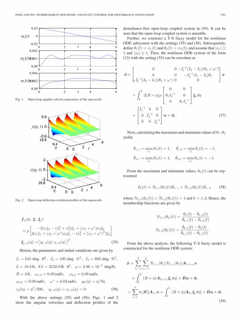
With the above settings (55) and (56), Figs. 1 and 2show the angular velocities and deflection profiles of the
disturbance-free open-loop coupled system in (54). It can beseen that the open-loop coupled system is unstable.
Further, we construct a T–S fuzzy model for the nonlinearODE subsystem with the settings (55) and (56). Subsequently,define θ1(t) = x1(t) and θ2(t) = x2(t), and assume that |x1 | ≤1 and |x2 | ≤ 1. Then, the nonlinear ODE system of the form(12) with the setting (55) can be rewritten as
x=
⎡
⎣0 0 −I−1
1 (I3 − I2)(θ2 + ω∗)0 0 −I−1
2 (I1 − I3)θ1−I−1
3 (I2 − I1)(θ2 + ω∗) 0 0
⎤
⎦x
+∫ L
02(R + η)ρ
⎡
⎢⎣
0 0θ1I
−12 0
0 θ1I−13
⎤
⎥⎦ ξtdη
+
⎡
⎢⎣
I−11 0 00 I−1
2 00 0 I−1
3
⎤
⎥⎦u+ d1 . (57)
Next, calculating the maximum and minimum values of θ1–θ2yields
θ1,1 = maxx1
θ1(t) = 1, θ1,2 = minx1
θ1(t) = −1,
θ2,1 = maxx2
θ2(t) = 1, θ2,2 = minx2
θ2(t) = −1.
From the maximum and minimum values, θk (t) can be rep-resented
θk (t) = Nk,1(θk (t))θk , 1 + Nk,2(θk (t))θk , 2 (58)
where Nk,1(θk (t)) + Nk,2(θk (t)) = 1 and k = 1, 2. Hence, themembership functions are given by
Nk,1(θk (t)) =θk (t) − θk ,2(t)θk ,1(t) − θk ,2(t)
Nk,2(θk (t)) =θk ,1(t) − θk (t)θk ,1(t) − θk ,2(t)
.
From the above analysis, the following T–S fuzzy model isconstructed for the nonlinear ODE system:
x =2∑
i1 =1
2∑
i2 =1
N1,i1 (θ1)N2,i2 (θ2)[A1,i1 i2x
+∫ L
0(R + η)A2,i1 i2 ξtdη] +Bu+ d1
=4∑
i=1
hi(θ)[A1,ix+∫ L
0(R + η)A2,iξtdη] +Bu+ d1
(59)
1302 IEEE TRANSACTIONS ON FUZZY SYSTEMS, VOL. 25, NO. 5, OCTOBER 2017
where hi(θ) =∏2
k=1 Nk,ik(θk ), i = 2(i1 − 1) + i2 , and
A1,i1 i2 =⎡
⎢⎣
0 0 −I−11 (I3 − I2)(θ2,i2 + ω∗)
0 0 −I−12 (I1 − I3)θ1,i1
−I−13 (I2 − I1)(θ2,i2 + ω∗) 0 0
⎤
⎥⎦
A2,i1 i2 = 2ρ
⎡
⎣0 0
θ1,i1I−12 0
0 θ1,i1I−13
⎤
⎦ , A1,i = A1,i1 i2 ,
A2, i = A2, i1 i2 , BΔ= diag{ I−1
1 , I−12 , I−1
3 }
ChooseC1 =diag{ 0.001, 0.001, 0.001}, C2 =diag{ 0.01,0.02},
R = 0,d1(t) =
{[ 0.04 0.1 0.05 ]T , 0 ≤ t ≤ 1s
0, others,
and
d2(η, t)=
{[d21(η, t) d22(η, t)
]T, t ∈ [0, 1], η ∈ [0, 18.8]
0, others
where d21(η, t) = 2(1 + 0.1η)−1 sin(0.1πt), and
d22(η, t) = 3(1 + η)−1sin(0.5πt).
Running the two-step design procedure via the MATLABLMI toolbox, the solutions to the optimization problem (52)can be obtained as
X =
⎡
⎣2.8978 × 10³ ∗ ∗6.3306 × 10⁻⁴ 10.0365 × 10³ ∗
−0.0921 0.6791 2.8254 × 10³
⎤
⎦
Q11 =[
2.6824 × 10⁻³ ∗−1.1171 × 10⁻¹² 2.1897 × 10⁻³
]
Q12 =[
2.3248 × 10⁻³ ∗−2.5788 × 10⁻¹² 1.6336 × 10⁻³
]
Q22 =[
0.0206 ∗−3.6691 × 10⁻¹⁰ 0.0123
]
Ks, 1 =
⎡
⎣−4.6961 × 10³ −8.7083 × 10⁻³ 2.8263
0.0238 −2.5235 × 10³ −11.68562.4975 2.8855 −4.7590 × 10³
⎤
⎦
Ks, 2 =
⎡
⎣−4.7893 × 10³ 8.9632 × 10⁻³ −2.7007
−0.0227 −2.5736 × 10³ −12.0202−2.3748 3.2013 −4.8532 × 10³
⎤
⎦
Fig. 3. Angular velocity trajectories of the spacecraft.
Ks, 3 =
⎡
⎢⎣
−4.8670 × 10³ 3.6336 × 10⁻³ 2.72871.9937 × 10−4 −2.6152 × 10³ 12.3502
2.3615 −3.0857 −4.9309 × 10³
⎤
⎥⎦
Ks, 4 =
⎡
⎢⎣
−4.9332 × 10³ −2.9877 × 10⁻³ −2.61931.2157 × 10−4 −2.6508 × 10³ 12.5967
−2.2603 −3.3207 −4.9980 × 10³
⎤
⎥⎦
Kb =[
1.1691 1.4527 × 10⁻⁸ 11.4037 1.7347 × 10⁻⁷
−1.6733 × 10⁻⁸ 1.5556 1.8661 × 10⁻⁷ 16.2077
]
α1 = 0.0738, α2 = 9.7833, α3 = 0.4991, γopt = 0.8004,
k1 = 1.0471 × 10⁻⁴ , k2 = 1.0833 × 10⁻⁶ ,
k3 = 1.1859 × 10⁻⁷ , k4 = 2.0528 × 10⁻³ .
Moreover, to show the merit of the proposed control method,we apply the control method in [16, Th. 3.1] for comparison.The corresponding feedback control laws are given as
up(t) = Ks, px(t), vp(t) = Bv (η)Kb, pξt(η, t) (60)
where vp(t) is a distributed controller as shown in [16, eq. (16)],in which
Ks, p = −diag{1000, 800, 1500}, Kb, p = −diag{ 10, 10}
Bv (η) = diag{b(η), b(η)}, b(η) ={
1, 17.86 ≤ η ≤ 18.8.0, else
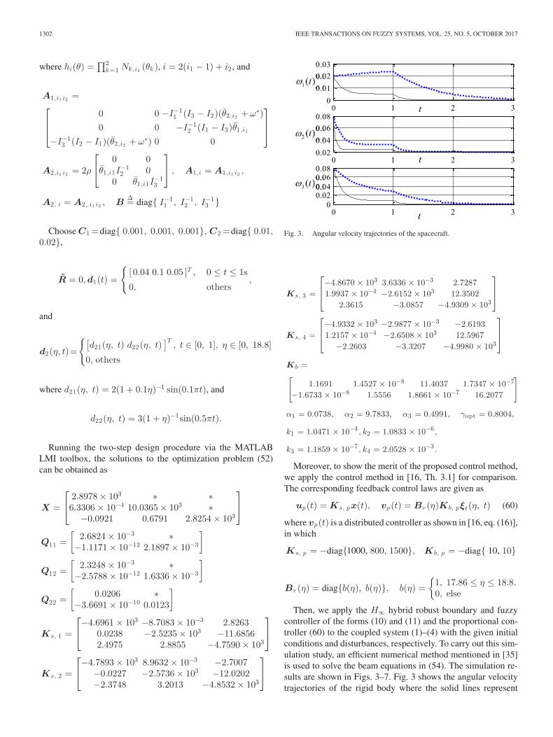
Then, we apply the H∞ hybrid robust boundary and fuzzycontroller of the forms (10) and (11) and the proportional con-troller (60) to the coupled system (1)–(4) with the given initialconditions and disturbances, respectively. To carry out this sim-ulation study, an efficient numerical method mentioned in [35]is used to solve the beam equations in (54). The simulation re-sults are shown in Figs. 3–7. Fig. 3 shows the angular velocitytrajectories of the rigid body where the solid lines represent
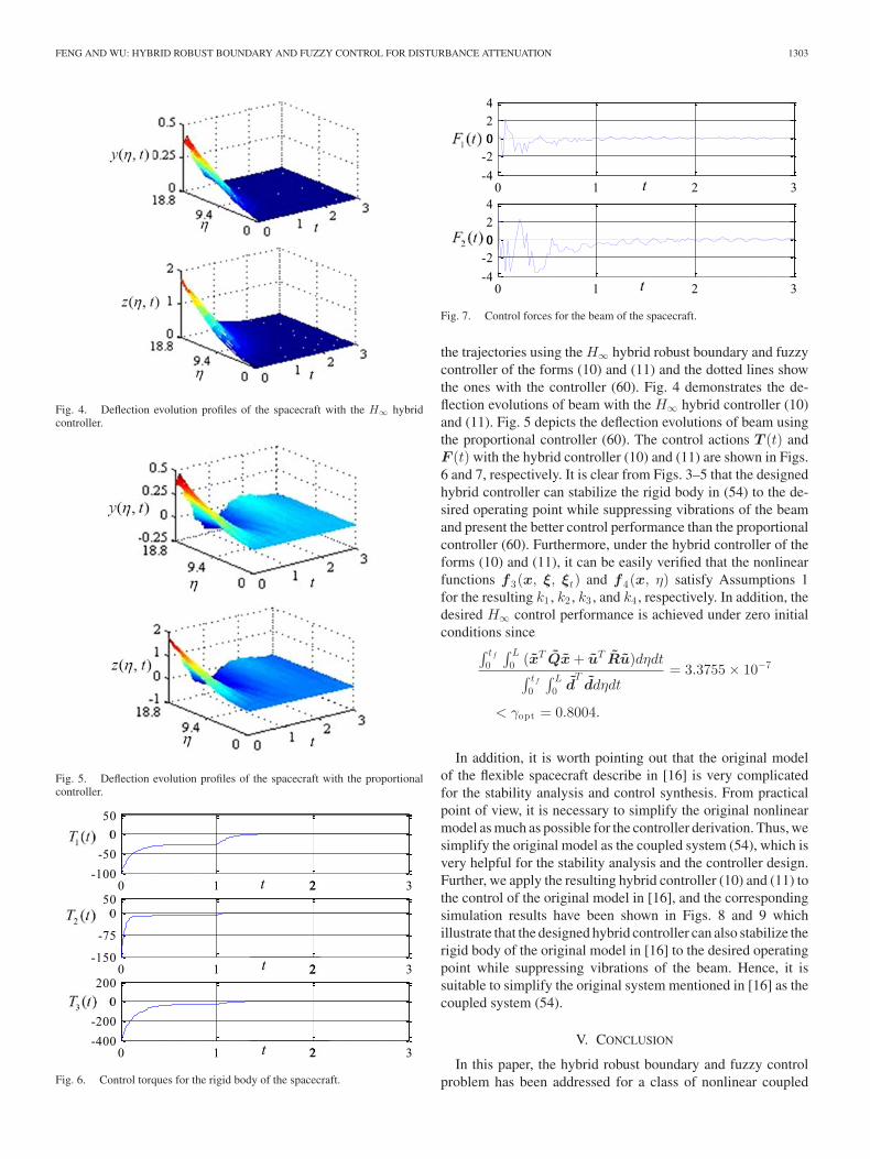
FENG AND WU: HYBRID ROBUST BOUNDARY AND FUZZY CONTROL FOR DISTURBANCE ATTENUATION 1303
Fig. 4. Deflection evolution profiles of the spacecraft with the H∞ hybridcontroller.
Fig. 5. Deflection evolution profiles of the spacecraft with the proportionalcontroller.
Fig. 6. Control torques for the rigid body of the spacecraft.
Fig. 7. Control forces for the beam of the spacecraft.
the trajectories using the H∞ hybrid robust boundary and fuzzycontroller of the forms (10) and (11) and the dotted lines showthe ones with the controller (60). Fig. 4 demonstrates the de-flection evolutions of beam with the H∞ hybrid controller (10)and (11). Fig. 5 depicts the deflection evolutions of beam usingthe proportional controller (60). The control actions T (t) andF (t) with the hybrid controller (10) and (11) are shown in Figs.6 and 7, respectively. It is clear from Figs. 3–5 that the designedhybrid controller can stabilize the rigid body in (54) to the de-sired operating point while suppressing vibrations of the beamand present the better control performance than the proportionalcontroller (60). Furthermore, under the hybrid controller of theforms (10) and (11), it can be easily verified that the nonlinearfunctions f 3(x, ξ, ξt) and f 4(x, η) satisfy Assumptions 1for the resulting k1 , k2 , k3 , and k4 , respectively. In addition, thedesired H∞ control performance is achieved under zero initialconditions since
∫ tf
0
∫ L
0 (xT Qx+ uT Ru)dηdt∫ tf
0
∫ L
0 dTddηdt
= 3.3755 × 10⁻⁷
< γopt = 0.8004.
In addition, it is worth pointing out that the original modelof the flexible spacecraft describe in [16] is very complicatedfor the stability analysis and control synthesis. From practicalpoint of view, it is necessary to simplify the original nonlinearmodel as much as possible for the controller derivation. Thus, wesimplify the original model as the coupled system (54), which isvery helpful for the stability analysis and the controller design.Further, we apply the resulting hybrid controller (10) and (11) tothe control of the original model in [16], and the correspondingsimulation results have been shown in Figs. 8 and 9 whichillustrate that the designed hybrid controller can also stabilize therigid body of the original model in [16] to the desired operatingpoint while suppressing vibrations of the beam. Hence, it issuitable to simplify the original system mentioned in [16] as thecoupled system (54).
V. CONCLUSION
In this paper, the hybrid robust boundary and fuzzy controlproblem has been addressed for a class of nonlinear coupled

1304 IEEE TRANSACTIONS ON FUZZY SYSTEMS, VOL. 25, NO. 5, OCTOBER 2017
Fig. 8. Angular velocity trajectories of the original model in [16] with thehybrid controller (10) and (11).
Fig. 9. Deflection evolution profiles of the original model in [16] with thehybrid controller (10) and (11).
ODE-beam systems with external disturbances via the robustand T–S fuzzy-model-based control techniques. A space-dependent BMI-based control design method is developedsuch that the closed-loop of the nonlinear coupled system isexponentially stable in the absence of the disturbances, and theH∞ control performance is guaranteed in the presence of thedisturbances. Moreover, the suboptimal H∞ control problemis formulated as a BMI optimization problem to make thedisturbance attenuation level as small as possible. A two-stepprocedure is then presented to solve this BMI optimizationproblem. Finally, the proposed design method is applied to thecontrol of a flexible spacecraft, and the simulation results illus-trate the effectiveness of the proposed control method. Besides,the theoretical results have wide applications in practicalengineering such as helicopter rotor/blades and turbine blades.
ACKNOWLEDGMENT
The authors would like to thank the Associate Editor and theanonymous reviewers for their helpful comments and sugges-tions, which have improved the presentation of this paper.
REFERENCES
[1] V. Larson, P. Likins, and E. Marsh, “Optimal estimation and attitudecontrol of a solar electric propulsion spacecraft,” IEEE Trans. Aerosp.Electron. Syst., vol. AES-13, no. 1, pp. 35–47, Jan. 1977.
[2] W. He, S. S. Ge, B. V. E. How, Y. S. Choo, and K. Hong, “Robustadaptive boundary control of a flexible marine riser with vessel dynamics,”Automatica, vol. 47, no. 4, pp. 722–732, 2011.
[3] S. O. R. Moheimani and A. J. Fleming, Piezoelectric Transducers forVibration Control and Damping. Lindon, UT, USA: Springer-Verlag,2006.
[4] M. J. Balas, “Active control of flexible systems,” J. Optim. Theory Appl.,vol. 25, no. 3, pp. 415–436, 1978.
[5] Q. Hu and G. Ma, “Variable structure control and active vibration sup-pression of flexible spacecraft during attitude maneuver,” Aerosp. Sci.Technol., vol. 9, no. 4, pp. 307–317, 2005.
[6] N. Wang, H.-N. Wu, and L. Guo, “Coupling-observer-based nonlinearcontrol for flexible air-breathing hypersonic vehicles,” Nonlinear Dyn.,vol. 78, no. 3, pp. 2141–2159, 2014.
[7] Q. Hu, “Robust adaptive backstepping attitude and vibration control withL2 -gain performance for flexible spacecraft under angular velocity con-straint,” J. Sound Vib., vol. 327, no. 3–5, pp. 285–298, 2009.
[8] O. Morgul, “Orientation and stabilization of a flexible beam attached to arigid body: Planar motion,” IEEE Trans. Autom. Control, vol. 36, no. 8,pp. 953–962, Aug. 1991.
[9] B. Chentouf and J.-M. Wang, “Stabilization and optimal decay rate for anon-homogeneous rotating body-beam with dynamic boundary controls,”J. Math. Anal. Appl., vol. 318, no. 2, pp. 667–691, 2006.
[10] X. Zhao and G. Weiss, “Well-posedness, regularity and exact controlla-bility of the SCOLE model,” Math. Control, Signals, Syst., vol. 22, no. 2,pp. 91–127, 2010.
[11] X. Zhao and G. Weiss, “Suppression of the vibrations of wind turbinetowers,” IMA J. Math. Control Inform., vol. 28, no. 3, pp. 377–389, 2011.
[12] X. Chen, B. Chentouf, and J.-M. Wang, “Exponential stability of a non-homogeneous rotating disk-beam-mass system,” J. Math. Anal. Appl.,vol. 423, no. 2, pp. 1243–1261, 2015.
[13] W. He and S. S. Ge, “Dynamic modeling and vibration control of a flexiblesatellite,” IEEE Trans. Aerosp. Electron. Syst., vol. 51, no. 2, pp. 1422–1431, Apr. 2015.
[14] H.-N. Wu and J.-W. Wang, “Static output feedback control via PDE bound-ary and ODE measurements in linear cascaded ODE-beam systems,” Au-tomatica, vol. 50, no. 11, pp. 2787–2798, 2014.
[15] Y. Gao, H.-N. Wu, J.-W. Wang, and L. Guo, “Feedback control designwith vibration suppression for flexible air-breathing hypersonic vehicles,”Sci. China Inform. Sci., vol. 57, no. 3, pp. 032204:1–032204:14, 2014.
[16] S. K. Biswas and N. U. Ahmed, “Stabilization of a class of hybrid systemsarising in flexible spacecraft,” J. Optim. Theory Appl., vol. 50, no. 1,pp. 83–108, 1986.
[17] T. Takagi and M. Sugeno, “Fuzzy identification of systems and its ap-plications to modeling and control,” IEEE Trans. Syst., Man, Cybern.,vol. SMC-15, no. 1, pp. 116–132, Jan./Feb. 1985.
[18] K. Tanaka and H. O. Wang, Fuzzy Control Systems Design and Analysis:A Linear Matrix Inequality Approach. New York, NY, USA: Wiley, 2001.
[19] H. D. Tuan, P. Apkarian, T. Narikiyo, and Y. Yamamoto, “Parameterizedlinear matrix inequality techniques in fuzzy control system design,” IEEETrans. Fuzzy Syst., vol. 9, no. 2, pp. 324–332, Apr. 2001.
[20] G. Feng, Analysis and Synthesis of Fuzzy Control Systems: A Model BasedApproach. New York, NY, USA: Taylor & Francis, 2010.
[21] S. Boyd, L. Ghaoui, E. Feron, and V. Balakrishnan, Linear Matrix In-equalities in System and Control Theory. Philadelphia, PA, USA: SIAM,1994.
[22] K. Zhou, J. C. Doyle, and K. Glover, Robust and Optimal Control. Engle-wood Cliffs, NJ, USA: Prentice-Hall, 1996.
[23] B.-S. Chen and Y.-T. Chang, “Fuzzy state-space modeling and robustobserver-based control design for nonlinear partial differential systems,”IEEE Trans. Fuzzy Syst., vol. 17, no. 5, pp. 1025–1043, Oct. 2009.

FENG AND WU: HYBRID ROBUST BOUNDARY AND FUZZY CONTROL FOR DISTURBANCE ATTENUATION 1305
[24] H.-N. Wu, H.-Y. Zhu, and J.-W. Wang, “H∞ fuzzy control for a class ofnonlinear coupled ODE-PDE systems with input constraint,” IEEE Trans.Fuzzy Syst., vol. 23, no. 3, pp. 593–604, Jun. 2015.
[25] H.-N. Wu, J.-W. Wang, and H.-X. Li, “Design of distributed H∞ fuzzycontrollers with constraint for nonlinear hyperbolic PDE systems,” Auto-matica, vol. 48, no. 10, pp. 2535–2543, 2012.
[26] J.-W. Wang, H.-N. Wu, and H.-X. Li, “Distributed fuzzy control designof nonlinear hyperbolic PDE systems with application to nonisothermalplug-flow reactor,” IEEE Trans. Fuzzy Syst., vol. 19, no. 3, pp. 514–526,Jun. 2011.
[27] J.-W. Wang, H.-N. Wu, and H.-X. Li, “Fuzzy control design for nonlin-ear ODE-hyperbolic PDE-cascaded systems: A fuzzy and entropy-likeLyapunov function approach,” IEEE Trans. Fuzzy Syst., vol. 22, no. 5,pp. 1313–1324, Oct. 2014.
[28] P. Gahinet, A. Nemirovski, A. J. Laub, and M. Chilali, LMI ControlToolbox for Use With MATLAB. Natick, MA, USA: MathWorks Inc.,1995.
[29] Z. Liu and S. Zheng, Semigroups Associated With Dissipative Systems.Boca Raton, FL, USA: Chapman & Hall/CRC, 1999.
[30] B.-Z. Guo, “Riesz basis property and exponential stability of controlledEuler-Bernoulli beam equations with variable coefficients,” SIAM J. Con-trol Optim., vol. 40, no. 6, pp. 1905–1923, 2002.
[31] J.-W. Wang and H.-N. Wu, “Some extended Wirtinger’s inequalities anddistributed proportional-spatial integral control of distributed parame-ter systems with multi-time delays,” J. Franklin Inst., vol. 352, no. 10,pp. 4423–4445, 2015.
[32] K. C. Goh, L. Turan, M. G. Safonov, G. P. Papavassilopoulos, and J. H.Ly, “Biaffine matrix inequality properties and computational methods,” inProc. Am. Control Conf., Baltimore, MD, USA, 1994, pp. 850–855.
[33] L. E. Ghaoui, F. Oustry, and M. AitRami, “A cone complementaritylinearization algorithm for static output-feedback and related problems,”IEEE Trans. Autom. Control, vol. 42, no. 8, pp. 1171–1176, Aug. 1997.
[34] Y.-Y. Cao, J. Lam, and Y.-X. Sun, “Static output feedback stabilization:An LMI approach,” Automatica, vol. 34, no. 12, pp. 1641–1645, 1998.
[35] A. P. Tzes, S. Yurkovich, and F. D. Langer, “A method for solution of theEuler-Bernoulli beam equation in flexible-link robotic systems,” in Proc.IEEE Int. Conf. Syst. Eng., Fairborn, OH, USA, 1989, pp. 557–560.
Shuang Feng received the B.E. degree in automationfrom Shandong University, Jinan, China, in 2012.She is currently working toward the Ph.D. degree incontrol theory and control engineering from BeihangUniversity (formerly Beijing University of Aeronau-tics and Astronautics), Beijing, China.
Her research interests include distributed parame-ter systems, robust control, finite-time control, adap-tive control, fuzzy modeling and control, and theirapplications to hypersonic vehicles or flexible space-craft.
Huai-Ning Wu was born in Anhui, China, on Novem-ber 15, 1972. He received the B.E. degree in automa-tion from Shandong Institute of Building MaterialsIndustry, Jinan, China, in 1992 and the Ph.D. degreein control theory and control engineering from Xi’anJiaotong University, Xi’an, China in 1997.
From August 1997 to July 1999, he was a Postdoc-toral Research Fellow with the Department of Elec-tronic Engineering, Beijing Institute of Technology,Beijing, China. From December 2005 to May 2006,he was a Senior Research Associate with the De-
partment of Manufacturing Engineering and Engineering Management, CityUniversity of Hong Kong (CityU), Kowloon, Hong Kong. From October toDecember during 2006-2008 and from July to August in 2010, 2011 and 2013,he was a Research Fellow in CityU. Since August 1999, he has been with theSchool of Automation Science and Electrical Engineering, Beihang University(formerly Beijing University of Aeronautics and Astronautics), Beijing, China.He is currently a Professor with Beihang University. His current research inter-ests include robust control, fault-tolerant control, distributed parameter systems,and fuzzy/neural modeling and control.
Dr. Wu serves as an Associate Editor of the IEEE TRANSACTIONS ON FUZZY
SYSTEMS, and the IEEE TRANSACTIONS ON SYSTEMS, MAN & CYBERNETICS:SYSTEMS.