IEEE TRANSACTIONS ON ELECTROMAGNETIC COMPATIBILITY 1 …sunju.org/docs/lu2017highspeed.pdf · IEEE TRANSACTIONS ON ELECTROMAGNETIC COMPATIBILITY 1 High-Speed Channel Modeling with

IEEE TRANSACTIONS ON ELECTROMAGNETIC COMPATIBILITY 1

High-Speed Channel Modeling with MachineLearning Methods for Signal Integrity Analysis

Tianjian Lu, Member, IEEE, Ju Sun, Member, IEEE, Ken Wu, Member, IEEE,and Zhiping Yang, Senior Member, IEEE

Abstract—In this work, machine learning methods are appliedto high-speed channel modeling for signal integrity analysis. Lin-ear, support vector and deep neural network (DNN) regressionsare adopted to predict the eye-diagram metrics, taking advantageof the massive amounts of simulation data gathered from priordesigns. The regression models, once successfully trained, canbe used to predict the performance of high-speed channelsbased on various design parameters. The proposed learning-based approach saves complex circuit simulations and substantialdomain knowledge altogether, in contrast to alternatives thatexploit novel numerical techniques or advanced hardware tospeed up traditional simulations for signal integrity analysis. Ournumerical examples suggest that both support vector and DNNregressions are able to capture the nonlinearities imposed bytransmitter and receiver models in high-speed channels. Overall,DNN regression is superior to support vector regression inpredicting the eye-diagram metrics. Moreover, we also investigatethe impact of various tunable parameters, optimization methods,and data preprocessing on both the learning speed and theprediction accuracy for the support vector and DNN regressions.

Index Terms—Deep Neural Networks, Eye Diagram, High-Speed Channel, Machine Learning, Signal Integrity, SupportVector Regression.

I. INTRODUCTION

A high-speed, chip-to-chip system-level design as shown inFig. 1(a) entails intensive simulations prior to manufacturing,for both verification and optimization purposes. In the areaof signal integrity, there are two major types of simulationtechniques: electromagnetic solvers and circuit simulators [1].Electromagnetic solvers are often used to extract modelsfor high-speed interconnects such as IC packages, printedcircuit boards (PCBs), and connectors. To evaluate the per-formance at the system level, most high-speed designs usethe eye diagram. As shown in Fig. 2, the eye diagram iscreated by first segmenting and then overlaying the transientwaveforms obtained from a circuit simulator. In addition tomodel extraction, simulations are also performed to predict theimpact of manufacturing variances on signal integrity, becausevariations of design parameters during manufacturing mayalter the characteristics of a well-designed high-speed channel.Simulations invariably happen in many iterations and acrossvarious design stages. Consequently, substantial amounts ofsimulation data are generated.

Tianjian Lu, Ken Wu, and Zhiping Yang are with Google Inc., 1600Amphitheatre Pkwy, Mountain View, CA 94043, USA, e-mail: {tianjianlu,kenzwu, zhipingyang}@google.com.

Ju Sun is with the Mathematics Department of Stanford University,450 Serra Mall, Building 380, Stanford, CA 94305-2125, USA, e-mail:[email protected]

(a)

(b)

Fig. 1: (a) The topology of a high-speed channel and (b) thedesign parameters considered in this work.

Fig. 2: Illustration of eye height and width in an eye diagram.

The simulation techniques employed in characterizing high-speed channels for signal integrity can be computationallyexpensive. There are efforts in utilizing domain decompositionschemes and parallel computing to enhance the efficiency ofelectromagnetic solvers on model extraction [2], [3]. Model-order reductions techniques are also proposed to achieve a fastfrequency sweep in extracting models over a broadband [4],[5]. Moreover, there are approaches to efficiently generatingeye diagrams by utilizing shorter data patterns as inputs [6] orusing statistical methods [7].

In this paper, we take a different route and propose ad-dressing the efficiency issue by taking advantage of theexisting simulation data. A learning-based model is trainedon the prior data. Once the training is completed, we obtaina reasonable model characterizing the underlying high-speedchannel—performance metrics such as eye height and width


can be predicted from the trained model for varying designparameters. The proposed approach requires no complex cir-cuit simulations or substantial domain knowledge. The modeltraining can be achieved within a reasonable amount of timeover modern computing hardware, and the obtained modelscan be reused for future designs, which amortizes the trainingcost. Once the training concludes, prediction can be performedin a highly efficient manner.

We consider eight design parameters for a high-speed chan-nel in this work; they are tabulated in Fig. 1(b). We use eyeheight and eye width as the performance metrics, which aresystematically used to assess the system-level performance ofhigh-speed channels. The technical task here is to predict theeye height and eye width for given design specifications. Fora given high-speed channel, suppose there is a deterministicfunction that maps the design parameters to the eye height(width). The learning problem here is to learn this functionfrom the available data samples. In machine learning term,this is a regression problem.

We study three regression methods in this work, namely,linear regression [8], support vector regression (SVR) [9],and deep neural network (DNN) regression [10]. Due to thenonlinearity imposed by the transmitter and receiver models,linear regression, which assumes a linear model for the un-derlying function, fails to make accurate predictions of eyeheight and width. SVR is able to handle nonlinearities withkernel mappings [9], [11], [12]. However, DNN regression issuperior to SVR in terms of empirical prediction accuracy. 1

Deep neural networks have recently made great progressin selecting relevant results for web search, making recom-mendations in online shopping, identifying objects in images,and transcribing speeches into texts, to name a few [10], [14].To model high-speed channels, a DNN takes in raw designparameters as the input and passes them through layers oflinear and nonlinear transformations; see Fig. 4. With adequatenumber of such transformations, the DNN approximates theunderlying parameter-performance function reasonably well.The better performance of DNN over SVR observed in ournumerical examples may be partly explained by the universalapproximation property of DNN [15], which (roughly) saysany function with reasonable regularity can be approximatedwith controlled errors by DNN with appropriate parameters.

II. REGRESSION METHODS

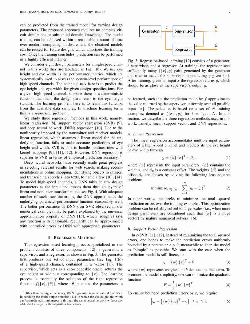
The regression-based learning process specialized to ourproblem consists of three components [12]: a generator, asupervisor, and a regressor, as shown in Fig. 3. The generatorfirst produces one set of input parameters (see Fig. 1(b))of a high-speed channel, contained in a vector {x}. Thesupervisor, which acts as a knowledgeable oracle, returns theeye height or width y corresponding to {x}. The learningprocess is essentially the selection of the right regressionfunction f({x}, {θ}), where {θ} contains the parameters to

1Other than the higher accuracy, DNN regression is more natural than SVRin handling the multi-output situation [13], in which the eye height and widthcan be predicted simultaneously through the same neural network without anyadditional change in the algorithm framework.

Fig. 3: Regression-based learning [12] consists of a generator,a supervisor, and a regressor. At training, the regressor seessufficiently many ({x}, y) pairs generated by the generatorand tries to match the supervisor in predicting y given {x}.After training, given an input x the regressor returns y, whichshould be as close as the supervisor’s output y.

be learned, such that the prediction made by f approximatesthe value returned by the supervisor uniformly over all possibleinput {x}. The selection is based on a set of N trainingexamples, denoted as ({xi}, yi) for i = 1, . . . , N . In thissection, we describe the three regression methods used in thiswork, namely, linear, support vector, and DNN regressions.

A. Linear Regression

The linear regression accommodates multiple input param-eters of a high-speed channel and predicts its the eye heightor eye width through

y = {β} {x}T+ β0, (1)

where {x} represents the input parameters, {β} contains theweights, and β0 is a constant offset. The weights {β} and theoffset β0 are chosen by solving the following least-squaresproblem:

minimize{β},β0

N∑i=1

(yi − yi)2 . (2)

In other words, one seeks to minimize the total squaredprediction errors over the training examples. This optimizationproblem can be reliably solved to large scales (i.e., when moredesign parameters are considered such that {x} is a hugevector) by mature numerical solvers [16].

B. Support Vector Regression

In ε-SVR [11], [12], instead of minimizing the total squarederrors, one hopes to make the prediction errors uniformlybounded by a parameter ε > 0, meanwhile to keep the modelas “simple” as possible. We start with the case when theprediction model is still linear, i.e.,

y = {w} {x}T+ b, (3)

where {w} represents weights and b denotes the bias term. Topromote the model simplicity, one can minimize the quadraticfunction

E =1

2{w} {w}T

. (4)

To ensure bounded prediction errors by ε, we require∣∣∣yi − ({w} {xi}T+ b)∣∣∣ ≤ ε, ∀ i. (5)


Together, we arrive at a convex optimization problem

minimize{w},b1

2{w} {w}T

subject to yi − {w} {xi}T − b ≤ ε, ∀ i,{w} {xi}T

+ b− yi ≤ ε, ∀ i.

(6)

For a pre-specified ε, there may not be a feasible linearfunction that obeys the constraints in (6). Slack variables {ξ}and {ξ∗} are hence introduced to add in flexibility; suchflexibility is meanwhile penalized in the objective, resultingin the notable ε-SVR formulation [12]:

minimize{w},b,{ξ},{ξ∗}

1

2{w} {w}T

+ C

N∑i=1

(ξi + ξ∗i )

subject to yi − {w} {xi}T − b ≤ ε+ ξi, ∀ i,{w} {xi}T

+ b− yi ≤ ε+ ξ∗i , ∀ i,ξi ≥ 0, ξ∗i ≥ 0, ∀ i,

(7)

where C is a tunable parameter to the optimization.For the above constrained convex optimization problem,

by introducing Lagrange multipliers to handle the inequalityconstraints and after simplification [11], we arrive at the dualproblem:

maximize g ({α}, {β})

subject to

N∑i=1

αi =

N∑i=1

βi, αi, βi ∈ [0, C] ∀ i,(8)

where the dual objective function is

g ({α}, {β}) = −1

2

N∑i=1

N∑j=1

(αi − βi) (αj − βj) {xi} {xj}T

− εN∑i=1

(αi + βi) +

N∑i=1

yi (αi − βi) . (9)

The prediction linear function in (3) can be written in termsof {α} and {β}:

y =

N∑i=1

(αi − βi) {xi} {x}T+ b. (10)

Maximization of the dual objective function in Equation (9)depends on the input vectors only through inner products ofthe form {xi}{xj}T. Similarly, the final prediction in Equa-tion (10) also depends on the input data only through innerproducts {xi}{x}T. To empower SVR to handle nonlinearity,a natural idea is to map the input vectors {xi} to a high-dimensional feature space through a nonlinear mapping, de-noted as Φ({xi}), and then feed these mapped vectors Φ({xi})into the linear model in Equation (3). This consequentlychanges the inner product terms in Equations (9) and (10)as:

{xi}{xj}T 7→ Φ ({xi}) Φ ({xj})T, ∀ i, j (11)

{xi}{x}T 7→ Φ ({xi}) Φ ({x})T, ∀ i. (12)

Due to the alluded sole dependency of Equations (9) and (10)on inner products, the kernel trick in SVR works by directlydefining an explicit kernel function K such that

K ({x}, {x′}) = ΦK ({x}) ΦK ({x′})T ∀ {x}, {x′} (13)

for a certain implicit nonlinear feature mapping ΦK . Applyingthe kernel trick, the dual objective function in Equation (9)becomes

− 1

2

N∑i=1

N∑j=1

(αi − βi) (αj − βj)K ({xi} , {xj})

− εN∑i=1

(αi + βi) +

N∑i=1

yi (αi − βi) (14)

and the prediction model in Equation (3) becomes

y =

N∑i=1

(αi − βi)K ({xi} , {x}) + b. (15)

The kernel trick avoids explicit calculation of the featuremapping and works by direct mapping to inner products.This often results in computational saving and allows im-plicit mapping into very high- or even infinite-dimensionalspaces [17]. The resulting problem is convex and can be solvedup to considerably large scales with specialized solvers; see,e.g., [18].

We study three kernels in this paper, namely, linear, poly-nomial, and Gaussian kernels. The linear kernel mapping issimply the identity mapping. An inhomogeneous polynomialkernel of degree d can be written as

K ({xi} , {xj}) =(

1 + {xi}T {xj})d. (16)

A Gaussian kernel is in the following form

K ({xi} , {xj}) = exp

(−|| {xi} − {xj} ||

2

2σ2

), (17)

where σ determines the bandwidth of the kernel that is tunable.The Gaussian kernel induces an implicit mapping that mapsthe input vectors into an infinite-dimensional space.

C. DNN Regression

As shown in Fig. 4(a), a feedforward neural network con-sists of many connected nodes in multiple layers. The numberof nodes belonging to individual layers can be lumped into avector {L} =

(Lin, L1, . . . , Lh, . . . , Ln, Lout

)where Lin, Lh,

Lout denote the number of nodes in the input layer, the hth

hidden layer, and the output layer, respectively. The input tothe hth hidden layer can be found through{

zh}

={xh−1

} [Wh

], (18)

where the Lh−1 × Lh matrix[Wh

]contains the weights

mapping output of the (h− 1)th layer to input of the hth layer.

The output vector {xh} of the hth hidden layer is obtained as

{xh} = fa({zh}

+ {bh}), (19)

where fa is a predefined scalar-to-scalar function that actselement-wise on the vector {zh}. Such fa is called the


(a)

(b)

Fig. 4: (a) A feedforward neural network typically consists ofone input layer, several hidden layers, and one output layer;(b) a node connects the (h − 1)th layer to the hth layer. Thew’s and b are the weights, and fa is the activation function.

activation function. The output from the final layer, i.e., {xout},is the prediction {y}. It is possible to return a vector directly;in this paper, for simplicity, we focus on returning a scalarvalue, i.e., when the output layer only consists of a singlenode.

The forms of nonlinear activation function considered inthis work include the rectified linear unit or ReLU [19]

fa(z) = max {0, z} , (20)

the hyperbolic tangent

fa(z) =ez − e−z

ez + e−z, (21)

and the sigmoid function

fa(z) =1

1 + e−z. (22)

Based on the input vector {xi}, the described feedforwardmechanism predicts the eye height or width {yi}, which differsfrom the true {yi} by

{ei} = {yi} − {yi}. (23)

To make {yi} a good approximation of {yi} uniformly overthe training examples, one minimizes the cost function

E =1

2

N∑i=1

{ei}{ei}T. (24)

Fig. 5: Comparison of the three different regression methodsin handling the nonlinearity imposed by the transmitter model.

The weights stored in matrices[Wh

]and vectors {bh} are

the optimization variables. To find a local minimum of thecost function, the stochastic gradient descent (SGD) methodis used, i.e.,[

Wh]

=[Wh

]− γ∇[Wh],{bh}E, ∀ h = 1, . . . , n,& out

(25)

where ∇[Wh],{bh}E is a stochastic approximation to the truegradient to ∇[Wh],{bh}E, and γ is called the learning rate, orthe step size parameter. The stochastic gradients ∇[Wh],{bh}Eare computed efficiently by the back-propagation method.

III. NUMERICAL EXAMPLES

In this section, we first evaluate the three regression methodsin terms of their capability of handling the nonlinearitiespresent in the high-speed channels. We then focus on SVRand DNN regression and investigate their performances ineye height and width prediction. As both SVR and DNNregression have many tunable components and parameters, wealso empirically study the impact of kernel selection on SVR,and likewise, activation function and optimization methodson DNN regression. Representation and quality of data arethe key determining factors on the effectiveness of machinelearning methods for practical problems [20]. Our experimentsdemonstrate that data preprocessing affects the convergencespeeds of numerical optimization methods on both SVR andDNN regression—when maximum number of iterations isenforced, this translates into different prediction accuraciesat the last iteration. Our implementation of SVR is basedon the scikit-learn [21] package, and DNN regression on theTensorFlow [22] package.

A. Comparison on Capability of Handling Nonlinearities

To generate the training set, we sweep the pre-emphasislevel on the transmitter side while fixing the remaining inputparameters and record the eye height. This simplifies the mul-tivariate regression problem into a univariate one. The training


Fig. 6: Performance of SVR in eye-height prediction withdifferent kernels. The polynomial kernel has degree three.

set thus contains only 10 examples, corresponding to all ad-missible pre-emphasis levels (Fig. 5). Linear regression cannothandle nonlinearities, which is evident from its formulationand the demonstration in Fig. 5—the predicted eye heightsby linear regression deviate significantly from the truth. BothSVR and DNN regression achieve excellent accuracy in eye-height prediction in the presence of nonlinearities. The DNNregression uses two hidden layers, each with 100 nodes. SVRwith different kernels can handle nonlinearities of differentforms and scales. As shown in Fig. 6, only Gaussian-kernelSVR successfully handles the nonlinearity in this numericalexample. Therefore, it is critical to select an appropriate kernelin order for SVR to accurately model the high-speed channel.

B. Performance of the DNN Regression

1 0 0 2 0 0 3 0 0 4 0 00

2

4

6

Relat

ive Er

ror (%

)

E x a m p l e s

Fig. 7: Relative errors of the predicted eye heights from theDNN regression on the test set.

In this section, we consider all the input parameters tab-ulated in Fig. 1(b) and investigate the performance of DNNregression for the complete multivariate regression.

A DNN is first trained to predict the eye height. Thetraining, validation, and test sets contain 717, 48, and 476

examples, respectively. The DNN has three hidden layers of100, 300, and 200 nodes, respectively. The learning rate ischosen as 0.01 and the batch size is 25. The maximum numberof iterations is set to 4000. The eye height in the data setvaries from 148 to 253 mV. Table I shows the predictionperformance measured by the root-mean-square error (RMSE)and the maximum relative error. The RMSE is defined as

RMSE =

√1

NRSS, (26)

where RSS is the least-squares objective function de-fined in Equation (2) and N is the number of exam-ples. Several variants of the SGD method are available;they often have different convergence speeds. With ourpre-specified maximum number of iterations, the differ-ent convergence speeds may translate into different pre-diction accuracies. We test three variants: the plain SGD(GradientDescentOptimizer in TensorFlow), the mo-mentum variant (MomentumOptimizer in TensorFlow),and the RMSProp variant (RMSPropOptimizer in Tensor-Flow) [23]. The RMSE on the training set with plain SGDis 3.1 mV and 3.4 mV on the test set. When the momentumvariant is used, the RMSE on the training set is reduced to1.9 mV and to 2.7 mV on the test set. Figure 7 depicts therelative errors of the predicted eye heights on the test set, andthe majority are below 3%.

Another DNN is trained to predict the eye width. The eyewidth is measured in unit intervals (UI)—one UI is definedas one data bit-width. The training, validation, and test setscontain 509, 35, and 203 examples, respectively. This DNNhas seven hidden layers of 10, 20, 20, 30, 20, 20, and 10nodes, respectively. The batch size is changed to 15. The eyewidth varies from 0.21 to 0.37 UI in the data set. From TableII, the RMSE with the momentum method is 0.006 UI on thetraining set and 0.008 UI on the test set, and the maximumrelative errors in both training and test sets are less than 10%.

0 1 0 0 0 2 0 0 0 3 0 0 0 4 0 0 00

5

1 0

1 5

2 0

RMSE

(mV)

S t e p s

G r a d i e n t D e s c e n t M o m e n t u m R M S P r o p

Fig. 8: Evolution of the RMSE of the predicted eye heightwith respect to the iteration index with the DNN regression.The three variants of SGD used in this paper are compared.

Figure 8 compares the convergence behaviors of the threevariants of SGD. The network architecture and common


TABLE I: Accuracy of predicted eye heights from the DNN regression.

Gradient Descent Momentum RMSProp

On Training SetRMSE (mV) 3.1 1.9 2.6

Maximum Relative Error (%) 6.2 4.1 5.2

On Test SetRMSE (mV) 3.4 2.7 3.1


TABLE II: Accuracy of predicted eye widths from the DNN regression. A unit interval (UI) is defined as one data bit-width,regardless of data rate. Eye width is measured in the UI.

Gradient Descent Momentum RMSProp

On Training SetRMSE (UI) 0.006 0.006 0.008


On Test SetRMSE (UI) 0.008 0.008 0.01


TABLE III: Accuracy of predicted eye heights from the SVR. Three different kernels are compared and the polynomial kernelhas degree three. The results shown here are after standardization is applied to the data set.

Gaussian Polynomial Linear

On Training SetRMSE (mV) 2.5 17.2 17.9


On Test SetRMSE (mV) 5.7 16.7 19.3


TABLE IV: Accuracy of predicted eye widths from the SVR with three different kernels. A unit interval (UI) is defined asone data bit-width, regardless of data rate. Eye width is measured in the UI. The results shown here are after standardizationis applied to the data set.

Gaussian Polynomial Linear

On Training SetRMSE (UI) 0.008 0.02 0.029


On Test SetRMSE (UI) 0.04 0.038 0.081


optimization parameters are tuned based on the hyperbolictangent activation and plain SGD. For the comparison, theseparameters are fixed and only the optimization methods arereplaced each time. The momentum variant works by accumu-lating gradient information across iterations, and the RMSRropvariant works by modifying the gradient and adaptively tuningthe learning rates. Our experiment suggests these heuristicsindeed lead to faster convergence.

Data preprocessing also influences the convergence speed.In the above experiments, individual input parameters were“standardized” to have zero mean and unit variance:

xnew =x− µσ

, (27)

where µ and σ are the empirical mean and standard deviationof the individual parameters, respectively. We compare thistype of preprocessing with data normalization

xnew =x− xmin

xmax − xmin(αmax − αmin) + αmin, (28)

which rescales the individual parameters into the interval[αmin, αmax]. Here xmin and xmax denote the minimum andmaximum values of the original data, respectively. Figure 9compares the impacts of data standardization, data normaliza-tion, and primitive input on the convergence speed. Both datastandardization and normalization significantly speed up theconvergence.


Fig. 9: Evolution of the RMSE of the predicted eye heightwith respect to the iteration index with the DNN regression.Three data preprocessing methods are compared.

Fig. 10: Evolution of the RMSE of the predicted eye heightwith respect to the iteration index with the DNN regression.Four different activation functions are compared.

Finally, we study the impact of different activation func-tions. Again, the network architecture and optimization pa-rameters are tuned based on the hyperbolic tangent activationand plain SGD, with the activation functions being replacedeach time. Figure 10 shows that the hyperbolic tangent andReLU enjoy faster convergence than the other two activationfunctions.

C. Performance of the SVR

We adopt the same training, validation, and test sets in theprevious section to analyze the prediction accuracy of SVR.The maximum number of iterations is set to 4000. As shown inTable III, the SVR with Gaussian kernel achieves a maximumrelative error of 10.2% on the test set in eye-height prediction,which is higher than that of the DNN regression. The instance-wise relative errors of the predicted eye heights with the SVRis depicted in Fig. 11. The relative errors for the majority ofexamples in the test set are below 6%. Similarly, for eye-widthprediction as shown in Table IV, the Gaussian-kernel SVR has

1 0 0 2 0 0 3 0 0 4 0 00

3

6

9

1 2

Relat

ive Er

ror (%

)

E x a m p l e s

Fig. 11: Relative errors of the predicted eye heights fromGaussian-kernel SVR on the test set.

Fig. 12: Evolution of the RMSE of the predicted eye heightwith respect to the iteration index. Convergence speed of theGaussian-kernel SVR is not sensitive to data standardization.

a maximum relative error of 23.4%, in contrast to the 10.6%by the DNN regression.

As for the impact of different kernels, the polynomial-kernelSVR does not make satisfactory predictions on eye height andthe maximum relative error is as high as 19.5% on test set.The linear SVR cannot handle the nonlinearities imposed bythe transmitter and receiver model, which is also shown inTables III and IV.

We also study the sensitivity of the convergence speed onSVR with respect to data preprocessing. We focus on theGaussian-kernel SVR due to its superior prediction accuracyas compared to other kernel choices. Figure 12 depicts theevolution of the RMSE of the predicted eye height with respectto the iteration index. The Gaussian-kernel SVR appears tobe insensitive to data standardization in our experiment, asthe evolution curves with and without the data standardizationroughly align with each other. However, data normalizationsubstantially slows down the convergence—in fact, empiricallythe Gaussian-kernel SVR seems to take forever to convergeafter the normalization.


IV. CONCLUSION AND DISCUSSION

In this work, we propose using machine learning methods topredict eye-diagram metrics of high-speed channels for signalintegrity analysis. Regression models are learned based on thelarge amount of prior simulation data. Once the learning iscompleted, the learned models can be used to predict the eyeheight and the eye width in future designs. This learning-based approach requires no substantial domain knowledge andmeanwhile saves complex and expensive circuit simulations.Through numerical examples, we studied three regressionmethods including linear, support vector, and DNN regressionson their capability of handling nonlinearities in the high-speed channels. We also studied the impacts of various tunableparameters including kernels in SVR, activation functionsand optimization methods in DNN regression, and two datapreprocessing schemes on the convergence speed at trainingand the prediction accuracy at testing.

Machine learning methods open an array of opportunitiesfor signal integrity analysis. As an immediate extension, theregression problem considered in this paper can be directlyformed as a classification problem, because eye masks arereadily available in many standard high-speed interfaces andhence the pass or fail labels are known. Another possibilityis to extend the current learning framework to analyze thefour-level pulse amplitude modulation (PAM-4) signaling,which is the leading contender for implementing high-speedchannels with 56 Gbps throughput and higher. In practice,simulation data are gathered over time as the design cycleprogresses. Therefore, it may be more appropriate to adopt anonline learning setting in which the channel models are beinggradually improved as new data become available. Finally,provided that adequate design data could be gathered, it isplausible to consider an “inverse design” setting, in which thetarget channel performance is specified and possible designparameter combinations are suggested by learning models.

REFERENCES

[1] S. H. Hall and H. L. Heck, Advanced signal integrity for high-speeddigital designs. John Wiley & Sons, 2011.

[2] J.-M. Jin, The finite element method in electromagnetics. John Wiley& Sons, 2015.

[3] Y. Li and J.-M. Jin, “A vector dual-primal finite element tearing andinterconnecting method for solving 3-D large-scale electromagneticproblems,” IEEE Transactions on Antennas and Propagation, vol. 54,no. 10, pp. 3000–3009, 2006.

[4] S. V. Polstyanko, R. Dyczij-Edlinger, and J.-F. Lee, “Fast frequencysweep technique for the efficient analysis of dielectric waveguides,”IEEE transactions on microwave theory and techniques, vol. 45, no. 7,pp. 1118–1126, 1997.

[5] S.-H. Lee, T.-Y. Huang, and R.-B. Wu, “Fast waveguide eigenanalysisby wide-band finite-element model-order reduction,” IEEE transactionson microwave theory and techniques, vol. 53, no. 8, pp. 2552–2558,2005.

[6] W.-D. Guo, J.-H. Lin, C.-M. Lin, T.-W. Huang, and R.-B. Wu, “Fastmethodology for determining eye diagram characteristics of lossy trans-mission lines,” IEEE Transactions on Advanced Packaging, vol. 32,no. 1, pp. 175–183, 2009.

[7] B. K. Casper, M. Haycock, and R. Mooney, “An accurate and efficientanalysis method for multi-gb/s chip-to-chip signaling schemes,” in VLSICircuits Digest of Technical Papers, 2002. Symposium on. IEEE, 2002,pp. 54–57.

[8] G. James, D. Witten, T. Hastie, and R. Tibshirani, An introduction tostatistical learning. Springer, 2013, vol. 112.

[9] H. Drucker, C. J. Burges, L. Kaufman, A. J. Smola, and V. Vapnik,“Support vector regression machines,” in Advances in neural informationprocessing systems, 1997, pp. 155–161.

[10] J. Schmidhuber, “Deep learning in neural networks: an overview,”Neural networks, vol. 61, pp. 85–117, 2015.

[11] A. J. Smola and B. Scholkopf, “A tutorial on support vector regression,”Statistics and computing, vol. 14, no. 3, pp. 199–222, 2004.

[12] V. Vapnik, The nature of statistical learning theory. Springer science& business media, 2013.

[13] H. Borchani, G. Varando, C. Bielza, and P. Larranaga, “A survey onmulti-output regression,” Wiley Interdisciplinary Reviews: Data Miningand Knowledge Discovery, vol. 5, no. 5, pp. 216–233, 2015.

[14] Y. LeCun, Y. Bengio, and G. Hinton, “Deep learning,” Nature, vol. 521,no. 7553, pp. 436–444, 2015.

[15] T. Poggio, H. Mhaskar, L. Rosasco, B. Miranda, and Q. Liao, “Why andwhen can deep-but not shallow-networks avoid the curse of dimension-ality: A review,” International Journal of Automation and Computing,pp. 1–17, 2017.

[16] S. Boyd and L. Vandenberghe, Convex optimization. Cambridgeuniversity press, 2004.

[17] A. J. Smola and B. Scholkopf, Learning with kernels. GMD-Forschungszentrum Informationstechnik, 1998.

[18] R.-E. Fan, P.-H. Chen, and C.-J. Lin, “Working set selection usingsecond order information for training support vector machines,” Journalof machine learning research, vol. 6, no. Dec, pp. 1889–1918, 2005.

[19] K. Jarrett, K. Kavukcuoglu, Y. LeCun et al., “What is the best multi-stage architecture for object recognition?” in Computer Vision, 2009IEEE 12th International Conference on. IEEE, 2009, pp. 2146–2153.

[20] S. Kotsiantis, D. Kanellopoulos, and P. Pintelas, “Data preprocessing forsupervised leaning,” International Journal of Computer Science, vol. 1,no. 2, pp. 111–117, 2006.

[21] F. Pedregosa, G. Varoquaux, A. Gramfort, V. Michel, B. Thirion,O. Grisel, M. Blondel, P. Prettenhofer, R. Weiss, V. Dubourg, J. Vander-plas, A. Passos, D. Cournapeau, M. Brucher, M. Perrot, and E. Duch-esnay, “Scikit-learn: Machine learning in Python,” Journal of MachineLearning Research, vol. 12, pp. 2825–2830, 2011.

[22] M. Abadi, A. Agarwal, P. Barham, E. Brevdo, Z. Chen, C. Citro, G. S.Corrado, A. Davis, J. Dean, M. Devin et al., “Tensorflow: large-scalemachine learning on heterogeneous distributed systems,” arXiv preprintarXiv:1603.04467, 2016.

[23] S. Ruder, “An overview of gradient descent optimization algorithms,”arXiv preprint arXiv:1609.04747, 2016.

Documents

IEEE TRANSACTIONS ON ELECTROMAGNETIC COMPATIBILITY 1 …sunju.org/docs/lu2017highspeed.pdf · IEEE TRANSACTIONS ON ELECTROMAGNETIC COMPATIBILITY 1 High-Speed Channel Modeling with