IEEE TRANSACTIONS ON COMPUTATIONAL INTELLIGENCE AND …zbyszek/PapersRB/Ahura-Car.pdf · IEEE TRANSACTIONS ON COMPUTATIONAL INTELLIGENCE AND AI IN GAMES 1 Ahura: A heuristic-based

IEEE TRANSACTIONS ON COMPUTATIONAL INTELLIGENCE AND AI IN GAMES 1

Ahura: A heuristic-based racer for the openracing car simulator

Mohammad Reza Bonyadi, Zbigniew Michalewicz, Samadhi Nallaperuma, Frank Neumann

Abstract—Designing automatic drivers for car racing isan active field of research in the area of robotics andartificial intelligence. A controller called Ahura (A HeUristic-based RAcer) for The Open Racing Car Simulator (TORCS)is proposed in this paper. Ahura includes five modules,namely steer controller, speed controller, opponent manager,dynamic adjuster, and stuck handler. These modules have 23parameters all together that are tuned using an evolutionarystrategy for a particular car to ensure fast and safe drive ondifferent tracks. These tuned parameters are further modifiedby the dynamic adjuster module during the run accordingto the width, friction, and dangerous zones of the track.The dynamic adjustment enables Ahura to decide on-the-fly based on the current situation, hence, it eliminates theneed for prior knowledge about the characteristics of thetrack. The driving performance of Ahura is compared withother state-of-the-art controllers on 40 tracks when they driveidentical cars. Our experiments indicate that Ahura performssignificantly better than other controllers in terms of damageand completion time especially on complex tracks (roadtracks). Also, experiments show that the overtaking strategyof Ahura is safer and more effective comparing to othercontrollers.

I. INTRODUCTION

DESIGNING a controller to drive a car is one of themost active research areas in the field of robotics

and artificial intelligence. Many well-known companiessuch as Audi and Google have been investing in thistopic and have gained some successes [1]. One of themain issues in this field of research is related to thedifficulty of accessing facilities such as sensors, actuators,and the vehicle itself mainly due to the expenses. Hence,a realistic simulator is a good candidate to replace theseresources and enable scientists to conduct research in thisarea. One of the most well-known car racing simulatorsis The Open Racing Car Simulator (TORCS) [2]. TORCSprovides many different cars (bots) that can be driventhrough a controller. Each bot provides all informationabout the environment (e.g., the whole track and exactposition of other cars) for the controller and the con-troller decides on the actuators (e.g., acceleration, brake,and clutch) accordingly. A more realistic extension of

All authors are with the Optimisation and Logistics Group,The University of Adelaide, Australia. M. R. Bonyadi ([email protected], [email protected]) and Z. Michalewiczare also with the data science group, Complexica, Adelaide, Australia.M. R. Bonyadi is also with the Centre for Advanced Imaging (CAI),the University of Queensland, Brisbane, QLD 4067, Australia. Z.Michalewicz is also with the Institute of Computer Science, PolishAcademy of Sciences, Warsaw, Poland, Polish-Japanese Institute ofInformation Technology, Warsaw, Poland.

TORCS has been designed [3]1 that includes ten morebots, each of these bots have been equipped by somelimited sensors to provide information about the car’senvironment at a fixed time rate (22ms in version 1.3.4of TORCS). The bot “listens” for actions such as acceler-ation, clutch, braking, gear, and steer from the controller.The provided actions by the controller are applied to thevehicle and cause the vehicle to act on the track.

In this paper, a new controller called Ahura (Aheuristic-based racer2) is proposed for TORCS. There arefive modules in Ahura: steer controller, speed controller,opponent manager, dynamic adjuster, and stuck handler.Each of these modules contain some parameters thatneed to be determined. The parameters for the steerand speed controllers are adjusted for a particular vehi-cle using the covariance matrix adaptation evolutionarystrategy (CMA-ES) [5] in a way that the controller drivesfast on the track while avoids actions that apply damageto the car. After setting these parameters, the parametersfor the opponent manager are set for that vehicle usinganother CMA-ES. This time, Ahura races against anothercontroller (called Blocker) that has been designed toblock the vehicle behind. The objective is to overtakeBlocker with the smallest amount of damage in a limitedtime. Ahura also uses a dynamic parameter adjustmentmodule that modifies the parameters of the controllerduring the race to perform according to mechanicalspecifications of the track.

There are four main features that make Ahura moresuccessful comparing to the existing controllers (e.g., [6],[7], [8]):

1) Ahura evaluates the direction of the turn in frontand prepares the vehicle’s position (tentative po-sition) at the track so that the centrifugal force isminimized while turning. This in fact increases themaximum safe speed (the speed that the vehicle canmove with while it still does not leave the track) fortaking the turn,

2) Ahura evaluates the angle of the turn in front andadjusts its acceleration policies to avoid unnecessarybrakes and dangerous acceleration. This enables thecontroller to make a better decision on the safe

1From here on, whenever we refer to TORCS, we refer to thisextension of the software rather than its original version. We used theversion 1.3.4 of this extension of TORCS [4].

2Ahura-Mazda is the name of a higher divine spirit of an old religioncalled Zoroastrianism. We picked the name Ahura because of therelation to the well-known vehicles brand ”Mazda”.


speed to take a turn,3) Ahura examines mechanical specifications (e.g., fric-

tion, boundaries, bumps) of the track during therun to adjust its driving decisions. This enables thecontroller to drive on a wide range of tracks,

4) Ahura evaluates all nearby opponents and generatesa spatial map of the opponents so that it can findappropriate slots to perform overtaking by changingits tentative position on the track. This enables thecontroller to avoid being blocked by the opponentsand overtake effectively,

The rest of this paper has been organized as follows.In section II we provide background information aboutTORCS and existing controllers. section III explains theproposed controller and its modules. Section IV com-pares Ahura with other controllers through some exper-iments, and section V concludes the paper.

II. BACKGROUND

In this section a brief background on The Open Rac-ing Car Simulator (TORCS) and existing controllers aregiven.

A. TORCS

TORCS is a well-known car racing simulator. There areten special bots in TORCS [3], [4] that are controllablethrough network ports by a client (controller). Thereare some (virtual) sensors connected to these bots thatobserve the environment and send the information tothe controller (see [3] for the full list and description ofthe sensors). There are 19 proximity sensors (the valueof the ith sensor is shown by disti) in front of thebot with predefined angles that provide the distancebetween the vehicle and the edges of the track towardstheir angle. The range of these sensors (shown by maxDin this paper) is 200 meters in the current version ofTORCS. The angle of the proximity sensor i is shownby anglei and it is a value in [−90, 90] degrees. Theseangles can be set at the beginning of the simulation.The index of the proximity sensor in front of the vehicleis 0 (called the zero sensor) and the index of the othersensors is set from −9 to 9. In the rest of this paper weassume anglex = angle−x. There are 36 opponent sensors(the value of the ith sensor is shown by oppi) that areonly sensitive to opponents. These sensors are all evenlydistributed around the bot with every 10 degrees (theindex of the sensor in front is 18) and their range is200 meters. There is a track position sensor (the valueis shown by trackPos) that provides a real value in theinterval [−∞,∞] (∞ refers to the maximum value of thetype double in computer), where −1 represents the rightside and 1 represents the left side of the track and othervalues translate to out of the track. There are 4 wheelspin sensors (one for each wheel) that calculate the speedof the wheels spin. The value for the wheel i is shown by

vi3 and it is in m/s. There is a rpm sensor that provides

the rotation per minutes of the engine and provides areal number in [0, 10000]. The current gear is an integerin {−1, 0, ..., 6} (−1 is the rear gear and 0 is the neutral)that is also provided. There are 3 sensors for the currentspeed of the vehicle along its front (the value is shownby xSpeed), sides (the value is shown by ySpeed), andabove (the value is shown by zSpeed). Finally, there is asensor that calculates the current damage of the vehiclethat is a real number in [0, 10000].

A controller should provide appropriate values forthe following actuators: acceleration pedal (shown byaccelPedal in this paper), braking pedal (shown bybrakePedal in this paper), and clutch pedal (shown byclutchV alue in this paper) that are real values in [0, 1],gear (shown by gearV alue in this paper) that is aninteger in {−1, 0, ..., 6}, and steer (shown by steerV aluein this paper) that is a real value in [−1, 1], correspondingto full right and full left. The decision by the controllershould be made within the simulation time interval (setto 22ms in the version 1.3.4 of TORCS). Hence, if thedesigned controller is slow then it might act by somedelays which may cause inappropriate movements.

B. Existing drivers for TORCS

There have been some drivers based on evolutionarystrategies, e.g., [8] and [7], for TORCS.

Cobostar [8] is a driver that maps sensory informationto actual motor behavior. It maps this information bya function that converts sensory information to desiredsteering angle and speed. The parameters of this func-tion are optimized by the covariance matrix adaptationevolutionary strategy (CMA-ES). Cobostar incorporatessome other heuristically designed features such as Anti-lock Braking System (ABS) and Anti-Slip Regulation(ASR), gear shifting, and recovery when stuck. Cobostarwon the simulated car racing competition at the Geneticand Evolutionary Computation Conference, GECCO,2008 (see http://cig.dei.polimi.it/ for the results of sim-ulated car racing competitions since 2008 at variousconferences).

MrRacer [7] uses an expert system approach for driv-ing. The basic design concept behind this driver isto use curvature estimation of a corner for setting atarget speed, and to use two modifiers that reduce theeffect of acceleration and brake in dependence of thecurrent steering angle. CMA-ES was used to optimizethe parameters of these functions. Additionally, MrRacerbuilds a track model during the warm up phase anduses this information during the race. The later versionsof MrRacer follow a rather offensive opponent handlingstrategy that tries to overtake the opponents in front andblocks the opponents behind. Furthermore, an online

3The radius of the wheels is available in the car dynamics files of thesimulator and, for the mentioned special cars in TORCS, it is 0.3179meters for the front wheels and 0.3276 meters for the rear wheels.

http://cig.dei.polimi.it/


adaptation is used by MrRacer to further adjust the pa-rameters (previously tuned in off-line mode) during thewarm up phase. MrRacer won the simulated car racingcompetition at the IEEE Computational intelligence andgames (CIG) conference, 2011.

Similar to MrRacer, EVOR [9] is a driver that makesuse of a track model built during the warm up phase.However, in contrast to the off-line parameter optimiza-tion strategy (e.g., in Cobostar and MrRacer), EVOR usesa dynamic optimization strategy to decide the actuatorvalues. A dynamic optimization process optimizes theactuator outputs based on the static track model andthe dynamic sensory information received during therace. The fitness function is based on how well the cartrajectory resultant from the current status informationsuits the track model. The opponent handing is alsoconsidered implicitly within this strategy that if oppo-nents intersect with the estimated trajectory they areconsidered as obstacles and the speed is adjusted toavoid any collision.

Autopia [6] is also an expert system quite similar toMrRacer and Cobostar. The significant difference be-tween this driver and the others mentioned before isthat it uses fuzzy inferencing to determine the targetspeed [10]. The parameters related to the driving func-tions are tuned using CMA-ES. Furthermore, Autopiaperforms online parameter adaptation during the warmup phase where the target speed is adapted based onthe damage. For example if the car is off the track at aposition then the target speed at this position is reduced.Autopia has rather a defensive opponent handling strat-egy that is designed heuristically. Autopia has won thesimulated car racing competition at various conferences,including CIG and GECCO 2010.

These four controllers are considered for the experi-ments in this study because they have shown good per-formance in the literature [8], [7], [6], [9] and they havebeen successful in several car racing competitions (seehttp://cig.dei.polimi.it/ for the results of simulated carracing competitions since 2008 at various conferences).There are also other controllers for TORCS based onexpert systems [11], [12], artificial neural networks [13],[14], fuzzy expert systems [15], [16], and genetic pro-gramming [17], [18], however, their performances are notas competitive as those four controllers.

Despite their competitive performance, these driversexhibit various drawbacks. For example, Cobostar andAutopia use the index of the proximity sensor that hasthe maximum value for the steer calculation, ignoringthe forces that the car experiences during the turn.However, these forces enforce the vehicle to move slowerduring the turn to avoid leaving the track. Also, noneof these controllers consider mechanical specifications ofthe track, such as friction, to adjust their driving style.However, such mechanical specifications of the tracksignificantly affect the safe speed as well as accelerationand braking performances of the vehicle. Although someof these information (e.g., friction) are not available

by sensors in TORCS, many of them can be estimatedreadily (see subsection III-E). Further, the fact that theproximity sensors have 200 meters of range has not beenused by any of these drivers while such information canbe useful to make better decisions on the speed andsteer of the vehicle. As an example, this range can beeffectively used to evaluate the turn in front and makebetter decisions. Finally, none of these controllers imple-ment effective overtaking strategy, e.g., Autpia tries toavoid the opponent and Cobostar just simply ignores theopponents. However, opponent handling is obviouslyessential in racing.

III. AHURA: A HEURISTIC-BASED RACER FOR TORCS

In this section we propose a new controller calledAhura for TORCS. The controller uses five modules:• Steer controller: this module uses the estimated

angle of the turn in front and the vacant distance infront to determine the steer angle. The module cancontrol how smooth or sharp the vehicle is going toturn.

• Speed controller: this module uses the estimatedturn angle together with the vacant distance in frontto decide the safe speed. In order to acceleratethe vehicle to achieve that speed, the controlleruses ASR/ABS technologies to avoid loosing thecontroller of the car.

• Opponent manager: this module creates a mapof opponents around and finds the vacant slot toovertake. This action may entail modification of thespeed and steer calculated by the speed and steercontroller modules.

• Dynamic adjuster: this module uses the mechanicalspecifications of the track (friction, bumps) as wellas recorded difficulties the controller has experi-enced during the earlier laps and adjusts the currentdriving style.

• Stuck manager: this module uses the idea proposedin [8] to control the vehicle when it is out of the trackor it has stuck somewhere.

These modules are described in detail in the followingsubsections.

A. Steer controller

Steer controller determines the value for the steer ofthe vehicle without considering opponents. The mainidea behind calculation of the steer angle is to find theproximity sensor that has the maximum empty space infront (called the base sensor), i.e., base sensor = {j|distj <disti, for any proximity sensor i}. The angle of thebase sensor (the value of anglebase sensor) is then usedto set the angle of the steer. However, moving exactlytowards the base sensor might cause some issues (seesubsection III-A2). Thus, the steer angle is calculatedaccording to the base sensor and some sensors around it,called auxiliary sensors. Although the steer angle should

http://cig.dei.polimi.it/


1q

2q1

dist

1dist

0dist

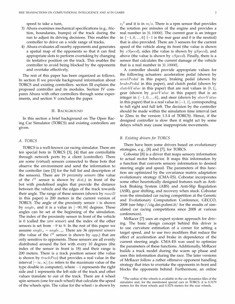
Fig. 1: The angle of the turn in front is estimated basedon dist−1,0,1 sensors.

Algorithm 1 Estimate the turn in frontInput: distOutput: estimatedTurn (estimated turn in front)

1: if dist1 > dist0 then2: k = sin(θ)dist1

dist0−cos(θ)dist13: else4: k = sin(θ)dist0

dist−1−cos(θ)dist05: end if6: estimatedTurn = tan−1(k)

be determined when the vehicle arrives to a turn, theaction before arriving to the turn is also important. Thus,the vehicle is prepared as soon as a turn was detected infront to take the turn with maximum speed and safety(see subsection III-A3). The preparation for turn involvesestimation of the angle of the turn in front. Hence, wedescribe the algorithm to estimate the angle of a turn insubsection III-A1.

1) Estimation of the angle of a turn: To estimate the angleof the turn in front we use three proximity sensors −1,0, and 1. Let us assume that the angle between thesesensors is θ (angle−1 = angle1 = θ). The angle of theturn (ϕ in Fig. 1) in front is calculated by tan−1( q2q1 ). Thevalue of q1 and q2 are calculated by dist−1 − cos(θ)dist0and sin(θ)dist0. Thus, Algorithm 1 is used to estimatethe turn in front.

Smaller values for θ lead to better estimations for thevalue of ϕ. The reason is that the proposed estimationprocedure uses two sample points on the edges of thetrack (provided by dist−1 and dist0 or dist1 and dist0) toestimate the angle of the turn. Thus, closer samples leadto more accurate calculation of the turn angle. Hence,we set θ = 1 in our experiments.

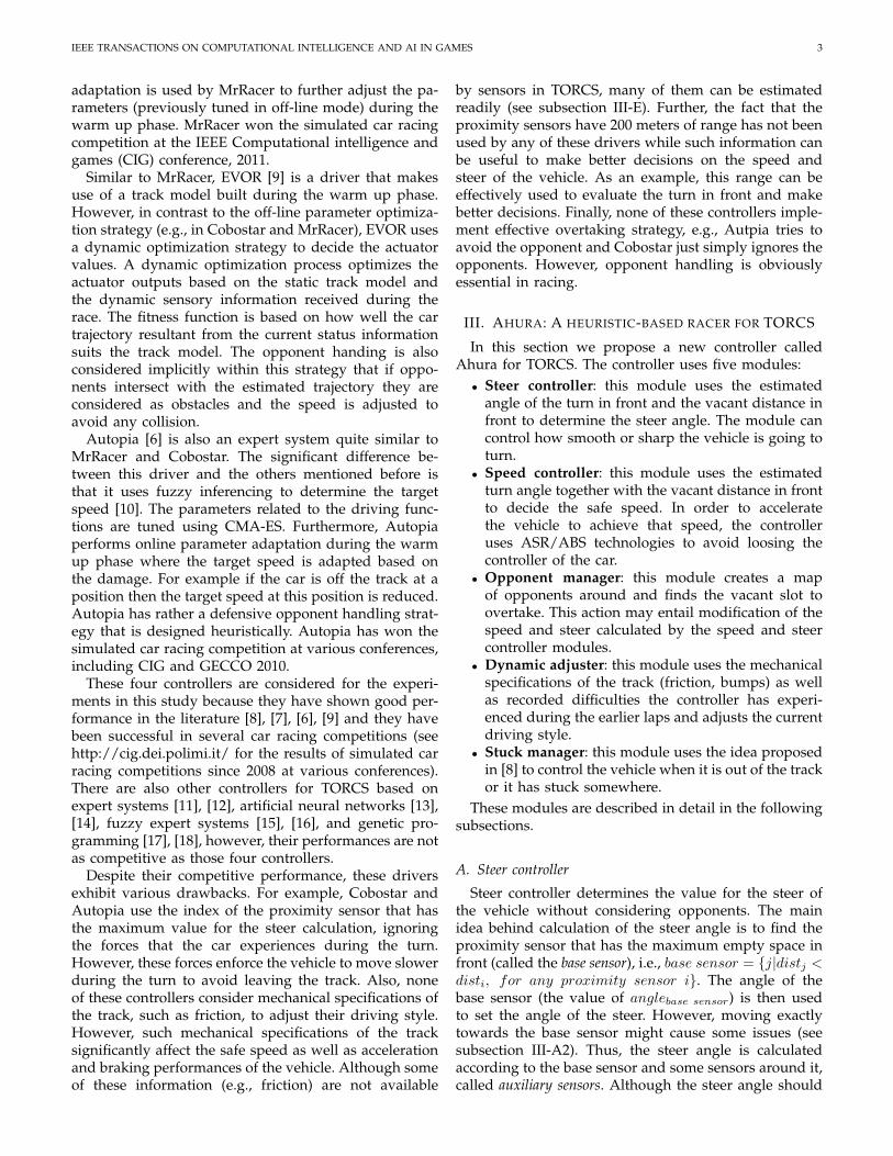
2) Taking a turn: The angle of the steer is set ac-cording to the angle of the base sensor (the value ofanglebase sensor). The trajectory towards the base sensor,however, might be very close to the edges of the trackthat might cause the vehicle to move out of the track.Also, if the angle between the base sensor and thedirection of movement is very large (a sharp turn) thensetting the steer angle to this large value might causelosing the control of the vehicle and slipping to the sidesof the track. To avoid these situations, the steer angle iscalculated according to a weighted average of the basesensor and some other sensors around it (see Fig. 2). We

Fig. 2: The red vector, the yellow vector, green vectors,and the blue vector represent the zero sensor, the basesensor, auxiliary sensors, and the final angle to take theturn, respectively.

call these extra sensors as auxiliary sensors.Because a weighted average over all auxiliary sensors

and the base sensor is used for calculation of the steerangle, the smoothness of the changes of the steer angleis a function of the number of auxiliary sensors. If thedistance in front of the vehicle is too small (dist0 issmall) then the vehicle needs to turn immediately andsharply. Thus, smaller number of sensors are preferred toenable the vehicle to change the direction more rapidly.However, if this distance is large then there is no needfor large and sudden changes of the steer angle. Hence,the number of auxiliary sensors is a function of dist0.We used a logarithm sigmoid function to map the valueof dist0 to the number of auxiliary sensors.

y = logSig(x1, x2, y1, y2, x) =a

1 + eb(x+c)+ d (1)

where x = dist0 and a, b, c, and d are defined as

a = y2 − y1

d = y1

b =ln( a

1.01y1−d−1)−ln( a0.99y2−d−1)

x1−x2

c =ln( a

1.01y1−d−1)

b − x1

(2)

With these settings4, the logarithm sigmoid functiongenerates 0.99y1 for dist0 = x1 and 0.99y2 for dist0 =

4There might be different ways to design a function to map dist0 tothe number of sensors, we designed this function manually. We need afunction f that maps the distance in front (x) to the number of sensors(y), i.e., y = f(x). The number of sensors should remain constant ifthe distance in front is larger than a value y2 or smaller than anothery1 (assuming y1 < y2). The reason is that the maximum number ofsensors is constant and the minimum number of sensors can not besmaller than 1. Hence, the function f has two asymptotes at y = y1and y = y2. If we assume that the minimum and maximum number ofauxiliary sensors are x1 and x2, respectively, then f(x1) should becomevery close to y1 and f(x2) should become very close to y2. Of courseone option for such function is a line that connects the points (x1, y1)and (x2, y2) when x ∈ [x1, x2] while has a constant value outside ofthe interval [x1, x2]. However, we experimentally found that the f(x)is not linear in the interval [x1, x2], hence, a logarithm sigmoid functionwas used. We assumed that f(x1) = y1 + 0.01y1 and f(x2) = y2 −0.01y2 (closer than 99% to y1 and y2 for x = x1 or x2, respectively).We then derived the values for a, b, c, and d accordingly.


Algorithm 2 Weighted average of the sensorsInputs: angle, dist, base sensor, α (a tentative position)Output: SteeringAnle (steer angle)

1: given x = dist0, calculate y by Eq. 12: L = {base sensor− y, ...base sensor, ..., base sensor+y}

3: h = g = 04: for each i in L do5: if i is the base sensor then6: d = 2disti7: else8: if anglei > anglebase sensor then9: d = disti

α10: else11: d = α× disti12: end if13: end if14: h = h+ d× cos(anglei)15: g = g + d× sin(anglei)16: end for17: steeringAngle = tan−1( gh )

x2. The total number of auxiliary sensors is 2y becausethe value y refers to the number of auxiliary sensors atone side of the base sensor (in our implementation, thenumber of auxiliary sensors is set to 2round(y) whereround(y) is the closest natural number to y). The valuesof y1, y2, x1, and x2 are the parameters that are tunedby an evolutionary strategy in section III-D.

During the run, x is substituted by dist0 in Eq.1 to calculate y. The value of y is then usedto generate a list L defined by {base sensor −y, ...base sensor, ..., base sensor+y} (see section III-A forthe calculation of the base sensor). The list L is used todetermine the steer angle by the algorithm 2.

The value of α in Algorithm 2 is the tentative positionof the vehicle at the track while moving. If α = 1.0 thenthe vehicle tends to stay in the middle of the track. If0.0 ≤ α ≤ 1.0 the distances that are at the left hand sideof the base sensor become larger (as they are divided by0.0 < α < 1.0) and the distances at the right hand side ofthe base sensor become smaller (as they are multipliedby 0.0 < α < 1.0). This multiplication/division resultsin more attraction towards the left hand side of thetrack. Also, if α > 1.0 the distances that are at theright hand side of the base sensor become larger andthe distances on the left hand side of the base sensorbecome smaller, resulting in more attraction towards theright hand side of the track. The value of distbase sensorhas been multiplied by 2 in the algorithm to increase theeffect of this sensor on the calculation of the steer angle.

3) Preparation for a turn: Although the steer angleshould be determined to take a turn, the action beforetaking the turn is also important because of the forcesthat the vehicle experiences during the turn. The vehicleexperiences a force during the turn outwards of the track

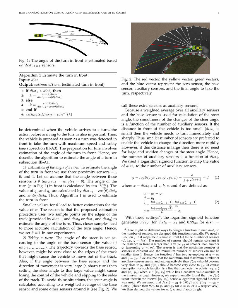
Fig. 3: Opposite sliding before the turn (red vector) incomparison to no sliding before the turn (white vector)

perpendicular to its body, called centrifugal force. Thecentrifugal force is proportional to the velocity, mass,and the angle of the steer (a small angle refers to asmooth turn and a large angle refers to a sharp turn),i.e., for a constant mass, the smaller the steer angleis, the smaller the force will be. Hence, for a constantmass and a constant centrifugal force, a smaller angleof steer allows larger velocity. Therefore, during a turn,if a smaller angle for the steer is selected then thevehicle is able to move faster while the centrifugal forceremains constant. In order to minimize the angle of thesteer (and consequently maximize the velocity) to takea turn the vehicle needs to take the largest curve that infact requires starting the turn from the further edge ofthe track (the red trajectory in Fig. 3). Thus, a strategyis needed to enable the vehicle to move towards theopposite side of the track before arriving to the turn andthen takes the turn. We call this strategy opposite sliding(see also [19]). Although a longer distance should thevehicle travel if this strategy is used (comparing to theother strategy in Fig. 3, shown by a white trajectory),the velocity that the vehicle can move by using thisstrategy is considerably larger than the other’s that notonly compensates for the larger distance, but also causessaving more time 5.

The opposite sliding in Ahura is implemented bysetting the value of α in Algorithm 2. Let us assumethat α = hsβ (h > 0)6, where s ∈ {−1, 1} determinesthe tentative position towards right/left side of the trackand β >= 0 determines the amplitude of the positiontowards the sides of the track. The value of s can bedetermined according to the estimated turn angle infront: if the turn is to the left (estimatedTurn < 0 inAlgorithm 1) then s = −1 to slide the vehicle to theright hand side of the track and vice versa.

The value of β is a function of the distance in front(dist0). The reason is that if dist0 is too large or too smallthen it is better to set α = 1.0 that entails setting β = 0.If dist0 is in the mid range then it is better to conductthe opposite sliding that needs α > 1.0 or α < 1.0(depending on the turn direction in front) that entails

5This strategy is also used by professional human drivers in racing.6Any positive value for h can be considered, however, we set this

value to 4 in our experiments.


β = 1.0 (note that the direction of the slide is determinedby s while β is only used to determine the amplitude ofthe slide). Hence, we used a trapezoidal function (Eq.3) to calculate appropriate value for β as a function ofdist0.

y = trap(a, b, c, d, x) =

0 x ≤ ax−ab−a a < x ≤ b1.0 b < x ≤ cc−xd−c + 1.0 c < x ≤ d0 x > d

(3)

where x = dist0, y = β, a is the distance where thevehicle should focus on taking the turn with no oppositesliding (β = 0 for x ≤ a), b is the distance where thevehicle should begin taking the turn and ending theopposite sliding (β drops from 1 to 0 for a < x ≤ b),c is the distance where the vehicle should be in theopposite sliding stage (β = 1 for any b < x ≤ c), andd is the distance where the opposite sliding stage begins(β grows from 0 to 1 for c < x ≤ d). The parameters a, b,c, and d are determined by an evolutionary strategy insection III-D.

As the opposite sliding procedure is not useful forwide angle turns, the value of β is set to zero if theestimated turn (determined by the Algorithm 1) is small.The threshold for the estimated angle of the turn to usethe opposite sliding is set to 0.1 in our experiments.

B. Speed controller

The aim of the speed controller is to determine thespeed that the vehicle can move by according to thecurrent situation without considering opponents. Thisdecision then is translated to the acceleration/breakingpedals.

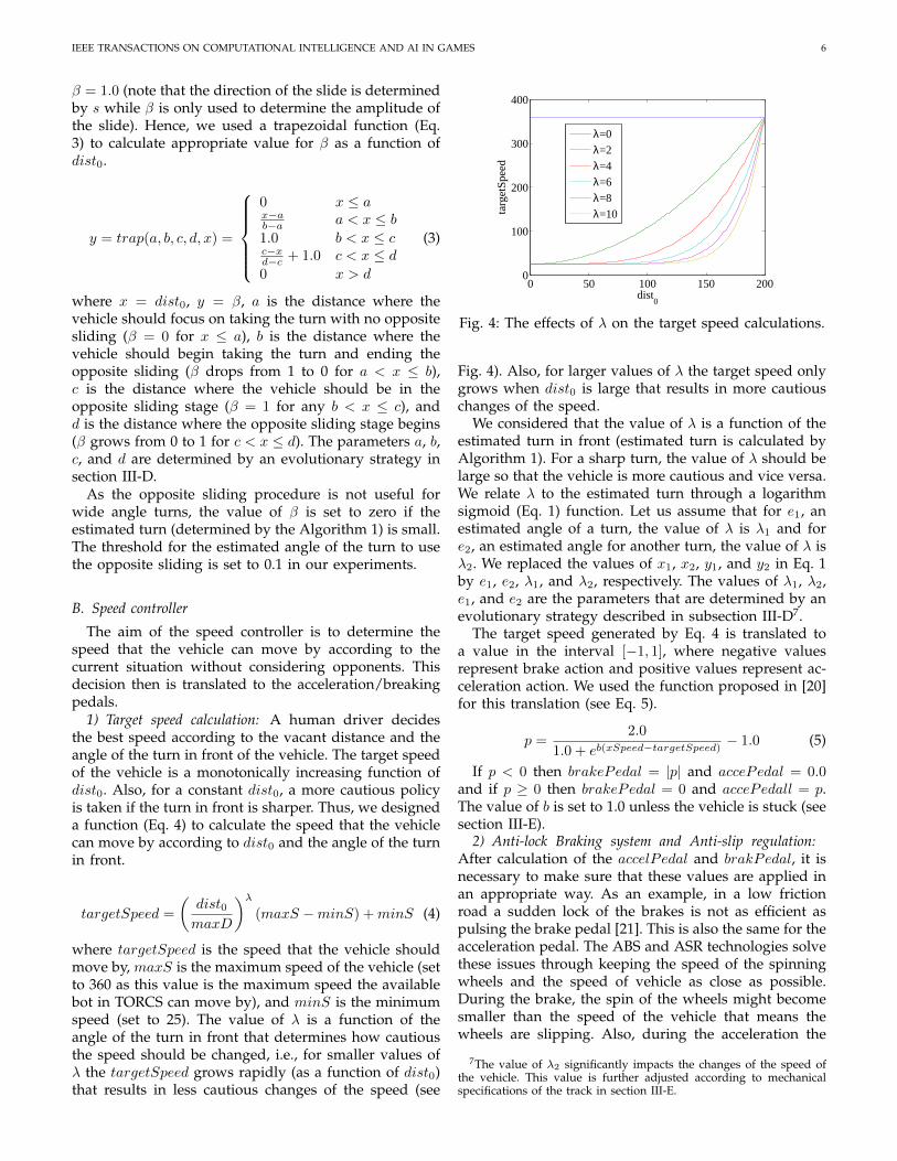
1) Target speed calculation: A human driver decidesthe best speed according to the vacant distance and theangle of the turn in front of the vehicle. The target speedof the vehicle is a monotonically increasing function ofdist0. Also, for a constant dist0, a more cautious policyis taken if the turn in front is sharper. Thus, we designeda function (Eq. 4) to calculate the speed that the vehiclecan move by according to dist0 and the angle of the turnin front.

targetSpeed =

(dist0maxD

)λ(maxS −minS) +minS (4)

where targetSpeed is the speed that the vehicle shouldmove by, maxS is the maximum speed of the vehicle (setto 360 as this value is the maximum speed the availablebot in TORCS can move by), and minS is the minimumspeed (set to 25). The value of λ is a function of theangle of the turn in front that determines how cautiousthe speed should be changed, i.e., for smaller values ofλ the targetSpeed grows rapidly (as a function of dist0)that results in less cautious changes of the speed (see

0 50 100 150 2000

100

200

300

400

dist0

targ

etSp

eed

λ=0λ=2λ=4λ=6λ=8λ=10

Fig. 4: The effects of λ on the target speed calculations.

Fig. 4). Also, for larger values of λ the target speed onlygrows when dist0 is large that results in more cautiouschanges of the speed.

We considered that the value of λ is a function of theestimated turn in front (estimated turn is calculated byAlgorithm 1). For a sharp turn, the value of λ should belarge so that the vehicle is more cautious and vice versa.We relate λ to the estimated turn through a logarithmsigmoid (Eq. 1) function. Let us assume that for e1, anestimated angle of a turn, the value of λ is λ1 and fore2, an estimated angle for another turn, the value of λ isλ2. We replaced the values of x1, x2, y1, and y2 in Eq. 1by e1, e2, λ1, and λ2, respectively. The values of λ1, λ2,e1, and e2 are the parameters that are determined by anevolutionary strategy described in subsection III-D7.

The target speed generated by Eq. 4 is translated toa value in the interval [−1, 1], where negative valuesrepresent brake action and positive values represent ac-celeration action. We used the function proposed in [20]for this translation (see Eq. 5).

p =2.0

1.0 + eb(xSpeed−targetSpeed)− 1.0 (5)

If p < 0 then brakePedal = |p| and accePedal = 0.0and if p ≥ 0 then brakePedal = 0 and accePedall = p.The value of b is set to 1.0 unless the vehicle is stuck (seesection III-E).

2) Anti-lock Braking system and Anti-slip regulation:After calculation of the accelPedal and brakPedal, it isnecessary to make sure that these values are applied inan appropriate way. As an example, in a low frictionroad a sudden lock of the brakes is not as efficient aspulsing the brake pedal [21]. This is also the same for theacceleration pedal. The ABS and ASR technologies solvethese issues through keeping the speed of the spinningwheels and the speed of vehicle as close as possible.During the brake, the spin of the wheels might becomesmaller than the speed of the vehicle that means thewheels are slipping. Also, during the acceleration the

7The value of λ2 significantly impacts the changes of the speed ofthe vehicle. This value is further adjusted according to mechanicalspecifications of the track in section III-E.


spin of the wheels might become larger than the speedof the vehicle that means the vehicle is in traction.

To implement ABS, we calculated the difference be-tween the speed of the vehicle and the speed that thewheels by d = |xSpeed−

∑4i=1 rivi|, ri is the radius of the

wheel i. If d is larger than ABSSlip then the value for thebrake pedal is revised to brakePedal− d−ABSSlip

ABSrange . Also, if∑4i=1 vi/4 is smaller than ABSMinSpeed then there is no

need to apply ABS as the vehicle is moving slowly. Theparameters ABSSlip, ABSrange, and ABSMinSpeedare determined to maximize the efficiency of the brakingsystem (see subsection III-D).

The implementation of ASR is very similar to thatof ABS. If d is larger than the maximum ASR speed(ASRSlip) then the value for the acceleration pedal isrevised to accelPedal+ ASRSlip−d

ASRrange (note that ASRSlip−dis negative, thus p becomes smaller). If the value of∑4i=1 vi/4 is larger than ASRMaxSpeed then p is not

changed. The parameters maxASR, ASRrange, andASRMaxSpeed are determined to maximize the effi-ciency of the acceleration system (see subsection III-D).

3) Gear control and clutch: We use a simple gearchanging procedure that is based on the minimumand maximum values of the rpm for each gear. Weset two thresholds for the motor’s rpm for each geari, one for the gear up (ui) and one for the geardown (di). The values for u1,...,6 and d1,...,6 were setto {9500, 9500, 9500, 9500, 9500, 0} (e.g., if gear=2 thenchange the gear to 3 if rpm is larger than u1 = 9500)and {0, 3300, 6200, 7000, 7300, 7700} (e.g., if gear=2 thenchange the gear to 1 if rpm is smaller than l2 = 3300)through some experiments.

The clutch is used to change the gears. However,clutch for the first gear is used in a special way byprofessional human drivers. When the gear is 1, theclutch is pushed half way through and it is releasedslowly in a way that the spin of the wheels remainsas close to the speed of the vehicle as possible. Thisprevents the wheels from slipping too much (maximizesthe friction between the wheels and the track surface) sothat the vehicle accelerates faster with less traction.

C. Opponent managerAhura’s opponent manager contains two modules,

steer reviser and speed reviser, that are responsible torevise steer and speed for overtaking. Ahura buildsa spacial map of the position of opponents based onthe information provided by the opp sensors. This mapis used to revise steer and speed of the vehicle forovertaking purposes.

1) Opponents spacial map: The information about op-ponents provided by opp sensors contain their distanceand angle from the current position of the vehicle. Thismeans that the position of opponents is provided in apolar coordinates system with the center of the measur-ing vehicle. Ahura builds a spacial map of the opponentspositions according to the given opp sensors. This map is

1

2

2

1

2

1

1d

2d

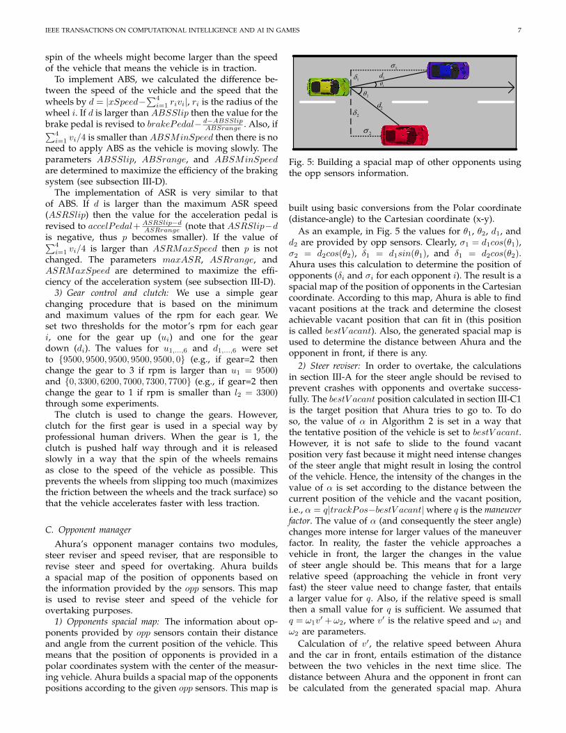
Fig. 5: Building a spacial map of other opponents usingthe opp sensors information.

built using basic conversions from the Polar coordinate(distance-angle) to the Cartesian coordinate (x-y).

As an example, in Fig. 5 the values for θ1, θ2, d1, andd2 are provided by opp sensors. Clearly, σ1 = d1cos(θ1),σ2 = d2cos(θ2), δ1 = d1sin(θ1), and δ1 = d2cos(θ2).Ahura uses this calculation to determine the position ofopponents (δi and σi for each opponent i). The result is aspacial map of the position of opponents in the Cartesiancoordinate. According to this map, Ahura is able to findvacant positions at the track and determine the closestachievable vacant position that can fit in (this positionis called bestV acant). Also, the generated spacial map isused to determine the distance between Ahura and theopponent in front, if there is any.

2) Steer reviser: In order to overtake, the calculationsin section III-A for the steer angle should be revised toprevent crashes with opponents and overtake success-fully. The bestV acant position calculated in section III-C1is the target position that Ahura tries to go to. To doso, the value of α in Algorithm 2 is set in a way thatthe tentative position of the vehicle is set to bestV acant.However, it is not safe to slide to the found vacantposition very fast because it might need intense changesof the steer angle that might result in losing the controlof the vehicle. Hence, the intensity of the changes in thevalue of α is set according to the distance between thecurrent position of the vehicle and the vacant position,i.e., α = q|trackPos−bestV acant|where q is the maneuverfactor. The value of α (and consequently the steer angle)changes more intense for larger values of the maneuverfactor. In reality, the faster the vehicle approaches avehicle in front, the larger the changes in the valueof steer angle should be. This means that for a largerelative speed (approaching the vehicle in front veryfast) the steer value need to change faster, that entailsa larger value for q. Also, if the relative speed is smallthen a small value for q is sufficient. We assumed thatq = ω1v

′ + ω2, where v′ is the relative speed and ω1 andω2 are parameters.

Calculation of v′, the relative speed between Ahuraand the car in front, entails estimation of the distancebetween the two vehicles in the next time slice. Thedistance between Ahura and the opponent in front canbe calculated from the generated spacial map. Ahura


records the changes of the distance of the opponent infront and uses the Lagrange interpolation technique with4 points [22] (set experimentally) to estimate the distancein the next simulation time slice (next 22ms). This esti-mation of the distance is then used to estimate the speedof the vehicle in front using the basic velocity calculationformula: v = x2−x1

t2−t1 where x2 is the extrapolated distance,x1 is the current distance, and t2 − t1 is the time sliceduration. If Ahura recognized that there is an opponenton one of its sides and it is vacant in front then thetentative position is kept constant until the opponent ispassed by a far enough distance.

Ahura determines the distance to start overtaking(shown by minDistToOvertake) according to the rela-tive speed with the vehicle in front. The faster Ahurais approaching the vehicle in front, the earlier it needsto overtake. We assumed that there is a linear re-lationship between minDistToOvertake and v′ , i.e.,minDistToOvertake = ω3v

′+ω4. If the distance from theopponent in front is smaller than minDistToOvertakethen Ahura starts changing the steer to overtake, other-wise, no action is taken. The parameters ω1, ω2, ω3, andω4 are set in section III-D.

If an opponent was detected and Ahura started toovertake, the number of auxiliary sensors (Algorithm 2)is set to maximum possible (10 in our implementations)to make the movement as accurate and smooth as possi-ble. In addition, if Ahura detected an opponent at eitherof its sides then the targetSpeed is multiplied by 1.1 tomake the overtaking process faster.

3) Speed reviser: The aim of the speed reviser is to re-vise targetSpeed to avoid crashes with other opponents.It is obvious that a vehicle A that is chasing a vehicle Bin front does not crash with B if it is moved at the samespeed or slower than B. Thus, Ahura estimates the speedof the vehicle in front in the next time slice and setsits own speed accordingly. To estimate the speed of thevehicle in front, the value of the current speed of Ahura(xSpeed) is added to the relative speed v′ (calculated insection III-C3). The targetSpeed is then set to the speedof the vehicle in front. The speed is revised only if thevehicle in front is closer than minDistToBrake = ω5,otherwise, it remains unchanged. The parameter ω5 isset in section III-D.

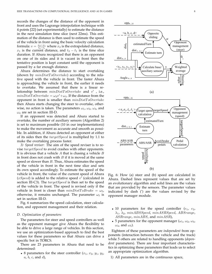
Fig. 6 summarizes the speed calculation, steer calcula-tion, and opponent management and their relation.

D. Optimization of parametersThe parameters for steer and speed controllers as well

as the opponent manager give Ahura the flexibility tobe able to drive a large range of vehicles. In this section,we use an optimization-based approach to find the bestvalues for these parameters so that Ahura can drive aspecific bot in TORCS.

There are 23 parameters in Ahura that need to bedetermined:• 8 parameters for the steer controller (x1, x2, y1, y2,a, b, c, and d),

Target speed calculation

ABS/ASR

1 2 1 2, , ,e e

ABS/ASR parameters

targetSp

Accel/bpeda

Accel/brake pedals

Estimateturn

dist-1, 0, 1

opp0...35

estimatedTurn

opp0...35

Estimate turn

Opposite sliding

Calculate base/auxiliary sensors

Opponent management

(steer)

Weighted average

'

dist-9...9

Steering angle

dist-1, 0, 1

<a, b, c, d>

<x1, x2, y1, y2>

estimatedTurn

y

dist

0

Angle-9...9

(a)

Target speed

calculation

Pedal

calculation

Opponent

management

(speed)

ABS/ASR

1 2 1 2, , ,e e

targetS

peed

'

ABS/ASR

parameters

targetSpeed

Accel/brake

pedals

Accel/b

rake

ped

als

Estimate

turn

dist-1, 0, 1

opp0...35

estimatedTurn

(b)

Fig. 6: How (a) steer and (b) speed are calculated inAhura. Dashed lines represent values that are set byan evolutionary algorithm and solid lines are the valuesthat are provided by the sensors. The parameter valuesindicated by dash (’) are the values revised by theopponent manager module.

• 10 parameters for the speed controller (e1, e2,λ1, λ2, minABSSpeed, minASRSpeed, ABSrange,ASRrange, minABS, and minASR),

• 5 parameters for the opponent manager (ω1, ω2, ω3,ω4, and ω5).

Eighteen of these parameters are independent from op-ponents (interaction between the vehicle and the track)while 5 others are related to handling opponents (depen-dent parameters). There are four important characteris-tics in optimizing these parameters that leads us to selectan appropriate optimization algorithm.

1) All parameters are in the continuous space,


TABLE I: Average and standard deviation of the objec-tive value over 10 runs (1 lap each) when the optimizedparamters for one track were tested on other tracks. Eachcolumn represents the average objective values (totaltime + damage/2) where Ahura used the parametersoptimized for the track specified in the heading of thatcolumn.

PWheel 2 PEroad PStreet 1 PAlpine 2Wheel 2 118.2 (0.29) 127.2 (1.22) 154.1 (1.41) 144.4 (2.09)

Eroad 69.7 (1.01) 68.2 (0.25) 73.8 (1.29) 79.2 (1.91)Street 1 130.4 (0.86) 135.3 (1.03) 87.7 (0.19) 109.6 (0.91)

Alpine 2 113.1 (0.92) 151.5 (1.04) 143.0 (1.11) 102.6 (0.24)Average 107.8 120.55 110.9 112.7

2) The effect of the changes of the value of parameterson the behavior of the vehicle is non-linear (chang-ing the value of λ affects the speed in a non-linearway, see Fig. 4),

3) There is no constraint,4) Some parameters are non–separable (changing the

value of one parameter changes the best possiblechoice for another), e.g., if the parameters are set ina way that the vehicle moves faster then the bestchoice for steering parameters are changed.

We use Covariance Matrix Adaptation EvolutionaryStrategy (CMA-ES) [5] for the optimization purposesbecause it has a good performance in continuous space,works with non-linear systems, no constraint handlingtechnique is required, and it is appropriate for non-separable search spaces [23].

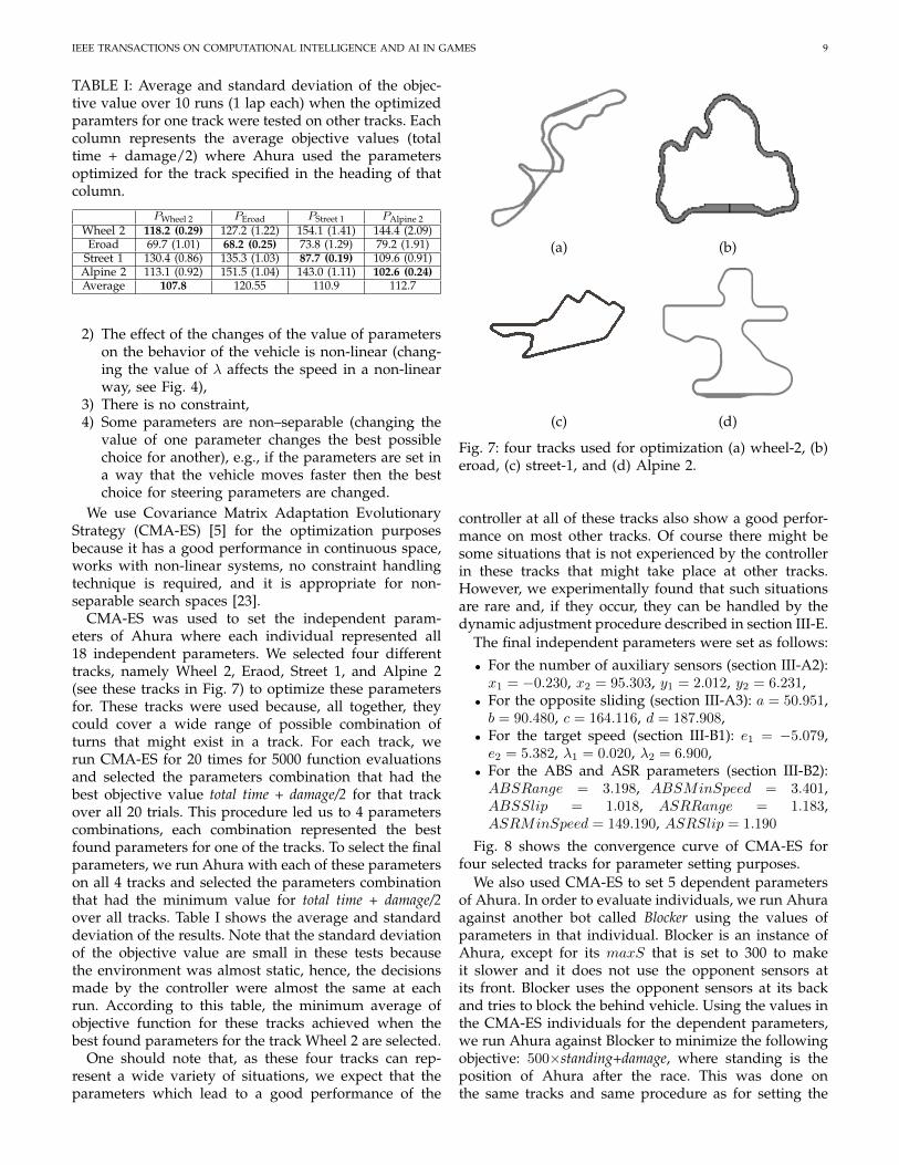
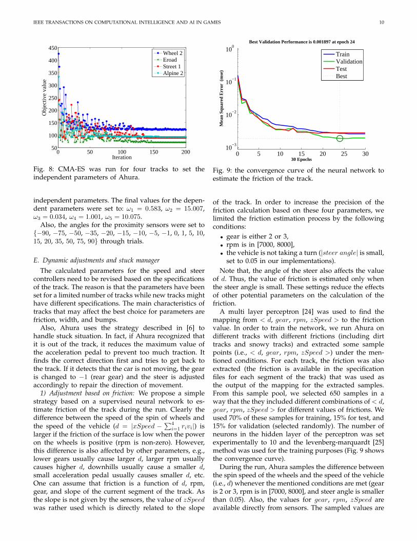
CMA-ES was used to set the independent param-eters of Ahura where each individual represented all18 independent parameters. We selected four differenttracks, namely Wheel 2, Eraod, Street 1, and Alpine 2(see these tracks in Fig. 7) to optimize these parametersfor. These tracks were used because, all together, theycould cover a wide range of possible combination ofturns that might exist in a track. For each track, werun CMA-ES for 20 times for 5000 function evaluationsand selected the parameters combination that had thebest objective value total time + damage/2 for that trackover all 20 trials. This procedure led us to 4 parameterscombinations, each combination represented the bestfound parameters for one of the tracks. To select the finalparameters, we run Ahura with each of these parameterson all 4 tracks and selected the parameters combinationthat had the minimum value for total time + damage/2over all tracks. Table I shows the average and standarddeviation of the results. Note that the standard deviationof the objective value are small in these tests becausethe environment was almost static, hence, the decisionsmade by the controller were almost the same at eachrun. According to this table, the minimum average ofobjective function for these tracks achieved when thebest found parameters for the track Wheel 2 are selected.

One should note that, as these four tracks can rep-resent a wide variety of situations, we expect that theparameters which lead to a good performance of the

(a) (b)

(c) (d)

Fig. 7: four tracks used for optimization (a) wheel-2, (b)eroad, (c) street-1, and (d) Alpine 2.

controller at all of these tracks also show a good perfor-mance on most other tracks. Of course there might besome situations that is not experienced by the controllerin these tracks that might take place at other tracks.However, we experimentally found that such situationsare rare and, if they occur, they can be handled by thedynamic adjustment procedure described in section III-E.

The final independent parameters were set as follows:

• For the number of auxiliary sensors (section III-A2):x1 = −0.230, x2 = 95.303, y1 = 2.012, y2 = 6.231,

• For the opposite sliding (section III-A3): a = 50.951,b = 90.480, c = 164.116, d = 187.908,

• For the target speed (section III-B1): e1 = −5.079,e2 = 5.382, λ1 = 0.020, λ2 = 6.900,

• For the ABS and ASR parameters (section III-B2):ABSRange = 3.198, ABSMinSpeed = 3.401,ABSSlip = 1.018, ASRRange = 1.183,ASRMinSpeed = 149.190, ASRSlip = 1.190

Fig. 8 shows the convergence curve of CMA-ES forfour selected tracks for parameter setting purposes.

We also used CMA-ES to set 5 dependent parametersof Ahura. In order to evaluate individuals, we run Ahuraagainst another bot called Blocker using the values ofparameters in that individual. Blocker is an instance ofAhura, except for its maxS that is set to 300 to makeit slower and it does not use the opponent sensors atits front. Blocker uses the opponent sensors at its backand tries to block the behind vehicle. Using the values inthe CMA-ES individuals for the dependent parameters,we run Ahura against Blocker to minimize the followingobjective: 500×standing+damage, where standing is theposition of Ahura after the race. This was done onthe same tracks and same procedure as for setting the


0 50 100 150 20050

100

150

200

250

300

350

400

450

Iteration

Obj

ectiv

e va

lue

Wheel 2EroadStreet 1Alpine 2

Fig. 8: CMA-ES was run for four tracks to set theindependent parameters of Ahura.

independent parameters. The final values for the depen-dent parameters were set to: ω1 = 0.583, ω2 = 15.007,ω3 = 0.034, ω4 = 1.001, ω5 = 10.075.

Also, the angles for the proximity sensors were set to{−90, −75, −50, −35, −20, −15, −10, −5, −1, 0, 1, 5, 10,15, 20, 35, 50, 75, 90} through trials.

E. Dynamic adjustments and stuck managerThe calculated parameters for the speed and steer

controllers need to be revised based on the specificationsof the track. The reason is that the parameters have beenset for a limited number of tracks while new tracks mighthave different specifications. The main characteristics oftracks that may affect the best choice for parameters arefriction, width, and bumps.

Also, Ahura uses the strategy described in [6] tohandle stuck situation. In fact, if Ahura recognized thatit is out of the track, it reduces the maximum value ofthe acceleration pedal to prevent too much traction. Itfinds the correct direction first and tries to get back tothe track. If it detects that the car is not moving, the gearis changed to −1 (rear gear) and the steer is adjustedaccordingly to repair the direction of movement.

1) Adjustment based on friction: We propose a simplestrategy based on a supervised neural network to es-timate friction of the track during the run. Clearly thedifference between the speed of the spin of wheels andthe speed of the vehicle (d = |xSpeed −

∑4i=1 rivi|) is

larger if the friction of the surface is low when the poweron the wheels is positive (rpm is non-zero). However,this difference is also affected by other parameters, e.g.,lower gears usually cause larger d, larger rpm usuallycauses higher d, downhills usually cause a smaller d,small acceleration pedal usually causes smaller d, etc.One can assume that friction is a function of d, rpm,gear, and slope of the current segment of the track. Asthe slope is not given by the sensors, the value of zSpeedwas rather used which is directly related to the slope

0 5 10 15 20 25 3010

−3

10−2

10−1

100

Best Validation Performance is 0.001897 at epoch 24

Mea

n Sq

uare

d E

rror

(m

se)

30 Epochs

TrainValidationTestBest

Fig. 9: the convergence curve of the neural network toestimate the friction of the track.

of the track. In order to increase the precision of thefriction calculation based on these four parameters, welimited the friction estimation process by the followingconditions:• gear is either 2 or 3,• rpm is in [7000, 8000],• the vehicle is not taking a turn (|steer angle| is small,

set to 0.05 in our implementations).Note that, the angle of the steer also affects the value

of d. Thus, the value of friction is estimated only whenthe steer angle is small. These settings reduce the effectsof other potential parameters on the calculation of thefriction.

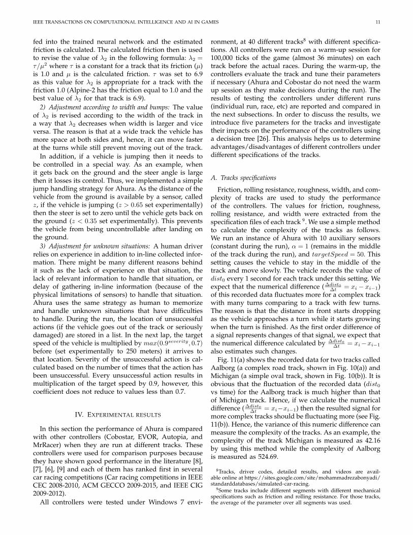
A multi layer perceptron [24] was used to find themapping from < d, gear, rpm, zSpeed > to the frictionvalue. In order to train the network, we run Ahura ondifferent tracks with different frictions (including dirttracks and snowy tracks) and extracted some samplepoints (i.e., < d, gear, rpm, zSpeed >) under the men-tioned conditions. For each track, the friction was alsoextracted (the friction is available in the specificationfiles for each segment of the track) that was used asthe output of the mapping for the extracted samples.From this sample pool, we selected 650 samples in away that the they included different combinations of < d,gear, rpm, zSpeed > for different values of frictions. Weused 70% of these samples for training, 15% for test, and15% for validation (selected randomly). The number ofneurons in the hidden layer of the perceptron was setexperimentally to 10 and the levenberg-marquardt [25]method was used for the training purposes (Fig. 9 showsthe convergence curve).

During the run, Ahura samples the difference betweenthe spin speed of the wheels and the speed of the vehicle(i.e., d) whenever the mentioned conditions are met (gearis 2 or 3, rpm is in [7000, 8000], and steer angle is smallerthan 0.05). Also, the values for gear, rpm, zSpeed areavailable directly from sensors. The sampled values are


fed into the trained neural network and the estimatedfriction is calculated. The calculated friction then is usedto revise the value of λ2 in the following formula: λ2 =τ/µ2 where τ is a constant for a track that its friction (µ)is 1.0 and µ is the calculated friction. τ was set to 6.9as this value for λ2 is appropriate for a track with thefriction 1.0 (Alpine-2 has the friction equal to 1.0 and thebest value of λ2 for that track is 6.9).

2) Adjustment according to width and bumps: The valueof λ2 is revised according to the width of the track ina way that λ2 decreases when width is larger and viceversa. The reason is that at a wide track the vehicle hasmore space at both sides and, hence, it can move fasterat the turns while still prevent moving out of the track.

In addition, if a vehicle is jumping then it needs tobe controlled in a special way. As an example, whenit gets back on the ground and the steer angle is largethen it losses its control. Thus, we implemented a simplejump handling strategy for Ahura. As the distance of thevehicle from the ground is available by a sensor, calledz, if the vehicle is jumping (z > 0.65 set experimentally)then the steer is set to zero until the vehicle gets back onthe ground (z < 0.35 set experimentally). This preventsthe vehicle from being uncontrollable after landing onthe ground.

3) Adjustment for unknown situations: A human driverrelies on experience in addition to in-line collected infor-mation. There might be many different reasons behindit such as the lack of experience on that situation, thelack of relevant information to handle that situation, ordelay of gathering in-line information (because of thephysical limitations of sensors) to handle that situation.Ahura uses the same strategy as human to memorizeand handle unknown situations that have difficultiesto handle. During the run, the location of unsuccessfulactions (if the vehicle goes out of the track or seriouslydamaged) are stored in a list. In the next lap, the targetspeed of the vehicle is multiplied by max(0.9severity, 0.7)before (set experimentally to 250 meters) it arrives tothat location. Severity of the unsuccessful action is cal-culated based on the number of times that the action hasbeen unsuccessful. Every unsuccessful action results inmultiplication of the target speed by 0.9, however, thiscoefficient does not reduce to values less than 0.7.

IV. EXPERIMENTAL RESULTS

In this section the performance of Ahura is comparedwith other controllers (Cobostar, EVOR, Autopia, andMrRacer) when they are run at different tracks. Thesecontrollers were used for comparison purposes becausethey have shown good performance in the literature [8],[7], [6], [9] and each of them has ranked first in severalcar racing competitions (Car racing competitions in IEEECEC 2008-2010, ACM GECCO 2009-2015, and IEEE CIG2009-2012).

All controllers were tested under Windows 7 envi-

ronment, at 40 different tracks8 with different specifica-tions. All controllers were run on a warm-up session for100,000 ticks of the game (almost 36 minutes) on eachtrack before the actual races. During the warm-up, thecontrollers evaluate the track and tune their parametersif necessary (Ahura and Cobostar do not need the warmup session as they make decisions during the run). Theresults of testing the controllers under different runs(individual run, race, etc) are reported and compared inthe next subsections. In order to discuss the results, weintroduce five parameters for the tracks and investigatetheir impacts on the performance of the controllers usinga decision tree [26]. This analysis helps us to determineadvantages/disadvantages of different controllers underdifferent specifications of the tracks.

A. Tracks specifications

Friction, rolling resistance, roughness, width, and com-plexity of tracks are used to study the performanceof the controllers. The values for friction, roughness,rolling resistance, and width were extracted from thespecification files of each track 9. We use a simple methodto calculate the complexity of the tracks as follows.We run an instance of Ahura with 10 auxiliary sensors(constant during the run), α = 1 (remains in the middleof the track during the run), and targetSpeed = 50. Thissetting causes the vehicle to stay in the middle of thetrack and move slowly. The vehicle records the value ofdist0 every 1 second for each track under this setting. Weexpect that the numerical difference ( ∆dist0

∆t = xi − xi−1)of this recorded data fluctuates more for a complex trackwith many turns comparing to a track with few turns.The reason is that the distance in front starts droppingas the vehicle approaches a turn while it starts growingwhen the turn is finished. As the first order difference ofa signal represents changes of that signal, we expect thatthe numerical difference calculated by ∆dist0

∆t = xi−xi−1

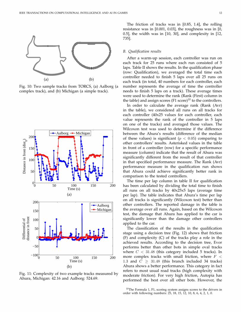
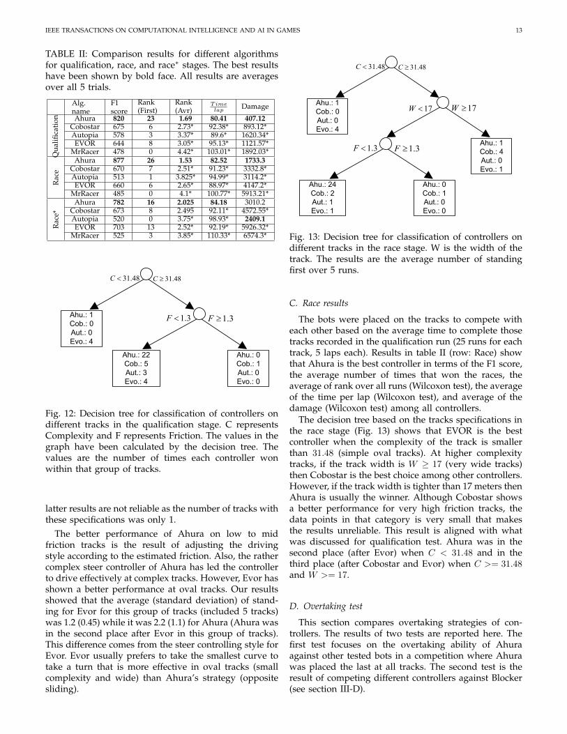
also estimates such changes.Fig. 11(a) shows the recorded data for two tracks called

Aalborg (a complex road track, shown in Fig. 10(a)) andMichigan (a simple oval track, shown in Fig. 10(b)). It isobvious that the fluctuation of the recorded data (dist0vs time) for the Aalborg track is much higher than thatof Michigan track. Hence, if we calculate the numericaldifference ( ∆dist0

∆t = xi−xi−1) then the resulted signal formore complex tracks should be fluctuating more (see Fig.11(b)). Hence, the variance of this numeric difference canmeasure the complexity of the tracks. As an example, thecomplexity of the track Michigan is measured as 42.16by using this method while the complexity of Aalborgis measured as 524.69.

8Tracks, driver codes, detailed results, and videos are avail-able online at https://sites.google.com/site/mohammadrezabonyadi/standarddatabases/simulated-car-racing.

9Some tracks include different segments with different mechanicalspecifications such as friction and rolling resistance. For those tracks,the average of the parameter over all segments was used.

https://sites.google.com/site/mohammadrezabonyadi/standarddatabases/simulated-car-racing

https://sites.google.com/site/mohammadrezabonyadi/standarddatabases/simulated-car-racing


(a) (b)

Fig. 10: Two sample tracks from TORCS, (a) Aalborg (acomplex track), and (b) Michigan (a simple track).

0 50 100 150 2000

50

100

150

200

Time (s)

Dis

tanc

e in

fro

nt (

dist

0)

Aalborg Michigan

(a)

0 50 100 150 200−100

−50

0

50

100

150

200

Time (s)

Diff

eren

tial o

f di

stan

ce in

fron

t

AalborgMichigan

(b)

Fig. 11: Complexity of two example tracks measured byAhura, Michigan: 42.16 and Aalborg: 524.69.

The friction of tracks was in [0.85, 1.4], the rollingresistance was in [0.001, 0.03], the roughness was in [0,0.5], the width was in [10, 30], and complexity in [12,735].

B. Qualification results

After a warm-up session, each controller was run oneach track for 25 runs where each run consisted of 5laps. Table II shows the results. In the qualification phase(row: Qualification), we averaged the total time eachcontroller needed to finish 5 laps over all 25 runs oneach track (in total, 40 numbers for each controller, eachnumber represents the average of time the controllerneeds to finish 5 laps on a track). These average timeswere used to determine the rank (Rank (First) column inthe table) and assign scores (F1 score)10 to the controllers.

In order to calculate the average rank (Rank (Avr)in the table), we considered all runs on all tracks foreach controller (40x25 values for each controller, eachvalue represents the rank of the controller in 5 lapson one of the tracks) and averaged those values. TheWilcoxon test was used to determine if the differencebetween the Ahura’s results (difference of the medianof these values) is significant (p < 0.05) comparing toother controllers’ results. Asterisked values in the tablein front of a controller (row) for a specific performancemeasure (column) indicate that the result of Ahura wassignificantly different from the result of that controllerin that specified performance measure. The Rank (Avr)performance measure in the qualification run showsthat Ahura could achieve significantly better rank incomparison to the tested controllers.

The time per lap column in table II for qualificationhas been calculated by dividing the total time to finishall runs on all tracks by 40x25x5 laps (average timeper lap). The table indicates that Ahura’s time per lapon all tracks is significantly (Wilcoxon test) better thanother controllers. The reported damage in the table isthe average over all runs. Again, based on the Wilcoxontest, the damage that Ahura has applied to the car issignificantly lower than the damage other controllersapplied to the car.

The classification of the results in the qualificationstage using a decision tree (Fig. 12) shows that friction(F) and complexity (C) of the tracks play a role in theachieved results. According to the decision tree, Evorperforms better than other bots in simple oval trackswhere C < 31.48 (this category included 5 tracks). Inmore complex tracks with small friction, where F <1.3 and C ≥ 31.48 (this branch included 34 tracks)Ahura shows a better performance. This category in factrefers to most usual road tracks (high complexity withmoderate friction). For very high friction, Autopia hasperformed the best over all other bots. However, the

10The Formula 1, F1, scoring system assigns scores to the drivers inorder with following numbers: 25, 18, 15, 12, 10, 8, 6, 4, 2, 1, 0.


TABLE II: Comparison results for different algorithmsfor qualification, race, and race∗ stages. The best resultshave been shown by bold face. All results are averagesover all 5 trials.

Alg.name

F1score

Rank(First)

Rank(Avr)

Timelap

Damage

Qua

lifica

tion Ahura 820 23 1.69 80.41 407.12

Cobostar 675 6 2.73* 92.38* 893.12*Autopia 578 3 3.37* 89.6* 1620.34*EVOR 644 8 3.05* 95.13* 1121.57*

MrRacer 478 0 4.42* 103.01* 1892.03*

Rac

e

Ahura 877 26 1.53 82.52 1733.3Cobostar 670 7 2.51* 91.23* 3332.8*Autopia 513 1 3.825* 94.99* 3114.2*EVOR 660 6 2.65* 88.97* 4147.2*

MrRacer 485 0 4.1* 100.77* 5913.21*

Rac

e*

Ahura 782 16 2.025 84.18 3010.2Cobostar 673 8 2.495 92.11* 4572.55*Autopia 520 0 3.75* 98.93* 2409.1EVOR 703 13 2.52* 92.19* 5926.32*

MrRacer 525 3 3.85* 110.33* 6574.3*

31.48C 31.48C

31.48C

1.3F 1.3F

Ahu.: 0Cob.: 1Aut.: 0Evo.: 0

31.48C


31.48C

1.3F 1.3F Ahu.: 1Cob.: 0Aut.: 0Evo.: 4


Fig. 12: Decision tree for classification of controllers ondifferent tracks in the qualification stage. C representsComplexity and F represents Friction. The values in thegraph have been calculated by the decision tree. Thevalues are the number of times each controller wonwithin that group of tracks.

latter results are not reliable as the number of tracks withthese specifications was only 1.

The better performance of Ahura on low to midfriction tracks is the result of adjusting the drivingstyle according to the estimated friction. Also, the rathercomplex steer controller of Ahura has led the controllerto drive effectively at complex tracks. However, Evor hasshown a better performance at oval tracks. Our resultsshowed that the average (standard deviation) of stand-ing for Evor for this group of tracks (included 5 tracks)was 1.2 (0.45) while it was 2.2 (1.1) for Ahura (Ahura wasin the second place after Evor in this group of tracks).This difference comes from the steer controlling style forEvor. Evor usually prefers to take the smallest curve totake a turn that is more effective in oval tracks (smallcomplexity and wide) than Ahura’s strategy (oppositesliding).

Aut.: 0Evo.: 0

31.48C 31.48C

17W Ahu.: 1Cob.: 0Aut.: 0Evo.: 4



1.3F 1.3F


17W

Fig. 13: Decision tree for classification of controllers ondifferent tracks in the race stage. W is the width of thetrack. The results are the average number of standingfirst over 5 runs.

C. Race results

The bots were placed on the tracks to compete witheach other based on the average time to complete thosetracks recorded in the qualification run (25 runs for eachtrack, 5 laps each). Results in table II (row: Race) showthat Ahura is the best controller in terms of the F1 score,the average number of times that won the races, theaverage of rank over all runs (Wilcoxon test), the averageof the time per lap (Wilcoxon test), and average of thedamage (Wilcoxon test) among all controllers.

The decision tree based on the tracks specifications inthe race stage (Fig. 13) shows that EVOR is the bestcontroller when the complexity of the track is smallerthan 31.48 (simple oval tracks). At higher complexitytracks, if the track width is W ≥ 17 (very wide tracks)then Cobostar is the best choice among other controllers.However, if the track width is tighter than 17 meters thenAhura is usually the winner. Although Cobostar showsa better performance for very high friction tracks, thedata points in that category is very small that makesthe results unreliable. This result is aligned with whatwas discussed for qualification test. Ahura was in thesecond place (after Evor) when C < 31.48 and in thethird place (after Cobostar and Evor) when C >= 31.48and W >= 17.

D. Overtaking test

This section compares overtaking strategies of con-trollers. The results of two tests are reported here. Thefirst test focuses on the overtaking ability of Ahuraagainst other tested bots in a competition where Ahurawas placed the last at all tracks. The second test is theresult of competing different controllers against Blocker(see section III-D).


92.50%

50.00%

17.50%

62.50%

30.00%

52.50%

70.00% 80.00%

67.50%

13.48%

29.76%

19.40%

43.79%

42.99%

5.99

%

7.29

%

11.97%

6.39

%

0.00%

20.00%

40.00%

60.00%

80.00%

100.00%

120.00%Win Damage

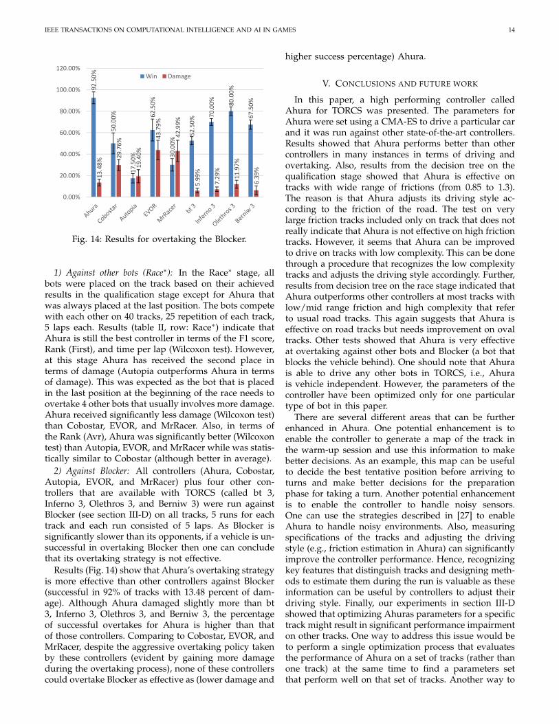
Fig. 14: Results for overtaking the Blocker.

1) Against other bots (Race∗): In the Race∗ stage, allbots were placed on the track based on their achievedresults in the qualification stage except for Ahura thatwas always placed at the last position. The bots competewith each other on 40 tracks, 25 repetition of each track,5 laps each. Results (table II, row: Race∗) indicate thatAhura is still the best controller in terms of the F1 score,Rank (First), and time per lap (Wilcoxon test). However,at this stage Ahura has received the second place interms of damage (Autopia outperforms Ahura in termsof damage). This was expected as the bot that is placedin the last position at the beginning of the race needs toovertake 4 other bots that usually involves more damage.Ahura received significantly less damage (Wilcoxon test)than Cobostar, EVOR, and MrRacer. Also, in terms ofthe Rank (Avr), Ahura was significantly better (Wilcoxontest) than Autopia, EVOR, and MrRacer while was statis-tically similar to Cobostar (although better in average).

2) Against Blocker: All controllers (Ahura, Cobostar,Autopia, EVOR, and MrRacer) plus four other con-trollers that are available with TORCS (called bt 3,Inferno 3, Olethros 3, and Berniw 3) were run againstBlocker (see section III-D) on all tracks, 5 runs for eachtrack and each run consisted of 5 laps. As Blocker issignificantly slower than its opponents, if a vehicle is un-successful in overtaking Blocker then one can concludethat its overtaking strategy is not effective.

Results (Fig. 14) show that Ahura’s overtaking strategyis more effective than other controllers against Blocker(successful in 92% of tracks with 13.48 percent of dam-age). Although Ahura damaged slightly more than bt3, Inferno 3, Olethros 3, and Berniw 3, the percentageof successful overtakes for Ahura is higher than thatof those controllers. Comparing to Cobostar, EVOR, andMrRacer, despite the aggressive overtaking policy takenby these controllers (evident by gaining more damageduring the overtaking process), none of these controllerscould overtake Blocker as effective as (lower damage and

higher success percentage) Ahura.

V. CONCLUSIONS AND FUTURE WORK

In this paper, a high performing controller calledAhura for TORCS was presented. The parameters forAhura were set using a CMA-ES to drive a particular carand it was run against other state-of-the-art controllers.Results showed that Ahura performs better than othercontrollers in many instances in terms of driving andovertaking. Also, results from the decision tree on thequalification stage showed that Ahura is effective ontracks with wide range of frictions (from 0.85 to 1.3).The reason is that Ahura adjusts its driving style ac-cording to the friction of the road. The test on verylarge friction tracks included only on track that does notreally indicate that Ahura is not effective on high frictiontracks. However, it seems that Ahura can be improvedto drive on tracks with low complexity. This can be donethrough a procedure that recognizes the low complexitytracks and adjusts the driving style accordingly. Further,results from decision tree on the race stage indicated thatAhura outperforms other controllers at most tracks withlow/mid range friction and high complexity that referto usual road tracks. This again suggests that Ahura iseffective on road tracks but needs improvement on ovaltracks. Other tests showed that Ahura is very effectiveat overtaking against other bots and Blocker (a bot thatblocks the vehicle behind). One should note that Ahurais able to drive any other bots in TORCS, i.e., Ahurais vehicle independent. However, the parameters of thecontroller have been optimized only for one particulartype of bot in this paper.

There are several different areas that can be furtherenhanced in Ahura. One potential enhancement is toenable the controller to generate a map of the track inthe warm-up session and use this information to makebetter decisions. As an example, this map can be usefulto decide the best tentative position before arriving toturns and make better decisions for the preparationphase for taking a turn. Another potential enhancementis to enable the controller to handle noisy sensors.One can use the strategies described in [27] to enableAhura to handle noisy environments. Also, measuringspecifications of the tracks and adjusting the drivingstyle (e.g., friction estimation in Ahura) can significantlyimprove the controller performance. Hence, recognizingkey features that distinguish tracks and designing meth-ods to estimate them during the run is valuable as theseinformation can be useful by controllers to adjust theirdriving style. Finally, our experiments in section III-Dshowed that optimizing Ahuras parameters for a specifictrack might result in significant performance impairmenton other tracks. One way to address this issue would beto perform a single optimization process that evaluatesthe performance of Ahura on a set of tracks (rather thanone track) at the same time to find a parameters setthat perform well on that set of tracks. Another way to


address this issue would be to find optimum parameterssets for Ahura for a set of tracks (one parameters setfor each track) and design a mechanism that identifieswhich of these parameters set is a better fit when thecontroller drives on a new track. This can be done byanalyzing the performance of the controller during thewarm-up stage when it uses different parameters set orby identifying how similar is the current track to otherpreviously evaluated tracks and use the best parametersset accordingly.

VI. ACKNOWLEDGMENT

This work was partially funded by the ARC DiscoveryGrant DP130104395 and by grant N N519 5788038 fromthe Polish Ministry of Science and Higher Education(MNiSW).

REFERENCES

[1] J. Markoff, “Google cars drive themselves, in traffic,” The NewYork Times, vol. 10, p. A1, 2010.

[2] B. Wymann, E. Espie, C. Guionneau, C. Dimitrakakis, R. Coulom,and A. Sumner, “TORCS, the open racing car simulator,” Softwareavailable at http://torcs.sourceforge.net, 2000.

[3] D. Loiacono, P. L. Lanzi, J. Togelius, E. Onieva, D. A. Pelta, M. V.Butz, T. D. Lonneker, L. Cardamone, D. Perez, and Y. Sez, “The2009 simulated car racing championship,” IEEE Transactions onComputational Intelligence and AI in Games, vol. 2, no. 2, pp. 131–147, 2010.

[4] D. Loiacono, L. Cardamone, and P. L. Lanzi, “Simulated car rac-ing championship: Competition software manual,” arXiv preprintarXiv:1304.1672, 2013.

[5] N. Hansen, S. Muller, and P. Koumoutsakos, “Reducing the timecomplexity of the derandomized evolution strategy with co-variance matrix adaptation (CMA-ES),” Evolutionary Computation,vol. 11, no. 1, pp. 1–18, 2003.

[6] E. Onieva, D. A. Pelta, J. Godoy, V. Milans, and J. Prez, “Anevolutionary tuned driving system for virtual car racing games:The AUTOPIA driver,” International Journal of Intelligent Systems,vol. 27, no. 3, pp. 217–241, 2012.

[7] J. Quadflieg, M. Preuss, and G. Rudolph, Driving faster than ahuman player. Springer, 2011, pp. 143–152.

[8] M. V. Butz and T. Lonneker, “Optimized sensory-motor couplingsplus strategy extensions for the torcs car racing challenge,” inComputational Intelligence and Games. IEEE, 2009, pp. 317–324.

[9] S. Nallaperuma, F. Neumann, M. R. Bonyadi, and Z. Michalewicz,“EVOR: an online evolutionary algorithm for car racing games,”in Genetic and evolutionary computation. ACM, pp. 317–324.

[10] E. Onieva, J. Godoy, J. Villagra, V. Milanes, and J. Perez, “On-linelearning of a fuzzy controller for a precise vehicle cruise controlsystem,” Expert Syst. Appl., vol. 40, no. 4, pp. 1046–1053, 2013.

[11] T. S. Kim, J. C. Na, and K. J. Kim, “Optimization of an autonomouscar controller using a self-adaptive evolutionary strategy,” Int JAdv Robot Syst, vol. 73, no. 9, 2012.

[12] J. Munoz, G. Gutierrez, and A. Sanchis, “A human-like TORCScontroller for the simulated car racing championship,” in Com-putational Intelligence and Games (CIG), 2010 IEEE Symposium on,2010, pp. 473–480.

[13] K.-J. Kim, J.-H. Seo, J.-G. Park, and J. C. Na, “Generalization ofTORCS car racing controllers with artificial neural networks andlinear regression analysis,” Neurocomp, vol. 88, pp. 87–99, 2012.

[14] D. Galanopoulos, C. Athanasiadis, and A. Tefas, “Evolution-ary optimization of a neural network controller for car racingsimulation.” in SETN, ser. Lecture Notes in Computer Science,I. Maglogiannis, V. P. Plagianakos, and I. P. Vlahavas, Eds., vol.7297. Springer, 2012, pp. 149–156.

[15] L. Cardamone, P. L. Lanzi, D. Loiacono, and E. Onieva, “Ad-vanced overtaking behaviors for blocking opponents in racinggames using a fuzzy architecture,” Expert Systems with Applica-tions, vol. 40, no. 16, pp. 6447–6458, 2013.

[16] D. Perez, G. Recio, Y. Saez, and P. Isasi, “Evolving a fuzzycontroller for a car racing competition,” in Proceedings of the 5thInternational Conference on Computational Intelligence and Games, ser.CIG’09. Piscataway, NJ, USA: IEEE Press, 2009, pp. 263–270.

[17] A. Agapitos, J. Togelius, and S. M. Lucas, “Evolving controllers forsimulated car racing using object oriented genetic programming,”in Genetic and evolutionary computation. ACM, 2007, pp. 1543–1550.

[18] J. Togelius, S. M. Lucas, H. D. Thang, J. M. Garibaldi,T. Nakashima, C. H. Tan, I. Elhanany, S. Berant, P. Hingston, R. M.MacCallum, T. Haferlach, A. Gowrisankar, and P. Burrow, “The2007 IEEE CEC simulated car racing competition,” Genetic Prog.and Evolvable Machines, vol. 9, no. 4, pp. 295–329, 2008.

[19] B. Beckman and N. B. R. Club, “The physics of racing, part 5:Introduction to the racing line,” online] http://www. esbconsult. com.au/ogden/locust/phors/phors05. htm, 1991.

[20] D. Galanopoulos, C. Athanasiadis, and A. Tefas, Evolutionaryoptimization of a neural network controller for car racing simulation.Springer, 2012, pp. 149–156.

[21] H. Pacejka, Tire and vehicle dynamics. Elsevier, 2005.[22] D. Sheen, “Introduction to numerical analysis,” 1980.[23] N. Hansen, R. Ros, N. Mauny, M. Schoenauer, and A. Auger,

“Impacts of invariance in search: When CMA-ES and pso face ill-conditioned and non-separable problems,” Applied Soft Computing,vol. 11, no. 8, pp. 5755–5769, 2011.

[24] F. Rosenblatt, “Principles of neurodynamics. perceptrons and thetheory of brain mechanisms,” DTIC Document, Tech. Rep., 1961.

[25] C. T. Kelley, Iterative methods for optimization. Siam, 1999, vol. 18.[26] J. R. Quinlan, “Learning decision tree classifiers,” ACM Computing

Surveys (CSUR), vol. 28, no. 1, pp. 71–72, 1996.[27] M. Preuss, J. Quadflieg, and G. Rudolph, “Torcs sensor noise

removal and multi-objective track selection for driving style adap-tation,” in IEEE Conference on Computational Intelligence and Games(CIG). IEEE, 2011, pp. 337–344.

Documents

IEEE TRANSACTIONS ON COMPUTATIONAL INTELLIGENCE AND …zbyszek/PapersRB/Ahura-Car.pdf · IEEE TRANSACTIONS ON COMPUTATIONAL INTELLIGENCE AND AI IN GAMES 1 Ahura: A heuristic-based