IEEE TRANSACTIONS ON AUTOMATIC CONTROL, … TRANSACTIONS ON AUTOMATIC CONTROL, VOL. X, NO. X, X 2014 1 Soft Constrained Model Predictive Control with Robust Stability Guarantees Melanie

IEEE TRANSACTIONS ON AUTOMATIC CONTROL, VOL. X, NO. X, X 2014 1

Soft Constrained Model Predictive Control withRobust Stability Guarantees

Melanie N. Zeilinger, Member, IEEE, Manfred Morari, Fellow, IEEE, and Colin N. Jones, Member, IEEE

Abstract—Soft constrained MPC is frequently applied in prac-tice in order to ensure feasibility of the optimization duringonline operation. Standard techniques offer global feasibility byrelaxing state or output constraints, but cannot ensure closed-loop stability. This paper presents a new soft constrained MPCapproach for tracking that provides stability guarantees evenfor unstable systems. Two types of soft constraints and slackvariables are proposed to enlarge the terminal constraint andrelax the state constraints. The approach ensures feasibilityof the MPC problem in a large region of the state space,depending on the imposed hard constraints, and stability isguaranteed by design. The optimal performance of the MPCcontrol law is preserved whenever all state constraints can beenforced. Asymptotic stability of all feasible reference steady-states under the proposed control law is shown, as well as input-to-state stability for the system under additive disturbances. Thesoft constrained method can be combined with a robust MPCapproach, in order to exploit the benefits of both techniques. Theproperties of the proposed methods are illustrated by numericalexamples.

Index Terms—Soft constraints, Model Predictive Control

I. INTRODUCTION

In control systems, there are generally two types of con-straints: those originating from physical limitations of theactuators or the system itself, including critical bounds relatedto, e.g., safe operation of the plant, or constraints derivedfrom desired system specifications. While input constraints cantherefore generally not be exceeded, state or output constraintscan either be hard if they fall under the first category, orthey can be considered soft. Violation may then in practicebe tolerated for short time periods, e.g. because of unexpecteddisturbances. Model predictive control (MPC) is a successfulparadigm for the control of constrained systems and offersguaranteed constraint satisfaction as well as stability in closed-loop, when all constraints are enforced in the MPC problem[1]. Imposing hard state or output constraints can, however,be overly conservative or render the optimization probleminfeasible in closed-loop operation. One possible remedy is tosimply remove the constraints for some portion of the predic-tion horizon until the problem becomes feasible. However, thismay lead to large constraint violations in closed-loop, when

M.N. Zeilinger is with the Department of Electrical Engineering andComputer Sciences, UC Berkeley, CA 94720, USA, and the Departmentof Empirical Inference, Max Planck Institute for Intelligent Systems, 72076Tübingen, Germany, email: [email protected].

C.N. Jones is with the Laboratoire d’Automatique, École PolytechniqueFédérale de Lausanne (EPFL), CH – 1015 Lausanne, Switzerland, email:[email protected].

M. Morari is with the Automatic Control Laboratory, ETH Zurich, CH –8092 Zurich, Switzerland, email: [email protected].

Manuscript received May 21, 2013; revised December 2, 2013.

implementing the first control input of the horizon, without anypossibility to tune the amount of violation. A popular approachis a so called soft constrained technique, where state or outputconstraints are relaxed and the size of the violation is penalizedin the cost. While this recovers feasibility of the MPC problemand offers the ability to tune the performance, standard softconstrained MPC schemes generally do not provide stabilityguarantees.

In this paper we propose a soft constrained linear MPCapproach for tracking that guarantees stability even for open-loop unstable systems. Although soft constraints are widelyused in practical implementations of MPC, this topic hasreceived comparably little attention in the literature. In [2],a condition on the quadratic penalty on the output constraintviolation is derived to guarantee stability for single-inputsingle-output systems. In [3], MPC with hard input and softoutput constraints is considered and stability is proven foropen-loop stable systems by showing that the stability proof inMPC extends to this case. This result also holds for marginallystable systems, if the horizon length is sufficiently long, whichis however difficult to choose in practice. The performanceof soft constrained MPC for relaxing output constraints wasinvestigated in [4]. The use of exact penalty functions in orderto enforce hard constraints when possible is discussed in [5],[6], in which case the stability properties are preserved in thefeasible set of the corresponding hard constrained problem. In[7], a Youla parametrization is employed and robust stabilityof the hard or soft constrained problem is enforced by addingan LMI to the MPC problem. The use of barrier functions toreplace constraints presented in [8] is a related idea, howeverthe key difference is that the barrier imposes a penalty insidethe constraint set, whereas in soft constrained schemes apenalty is only imposed on the constraint violation. As a result,this approach only provides stability in the feasible set of thecorresponding hard constrained problem.

The method proposed in this paper has the advantagethat it is conceptually similar to a standard soft constrainedtechnique usually applied in practice, but it also maintains thedesirable properties of MPC. Feasibility of the MPC problemis ensured in a large region of the state-space, which dependson the imposed hard constraints. Stability is guaranteed bydesign, while allowing to tune the system performance andthe amount of constraint violation. The method is based onthe MPC approach for tracking introduced in [9] and uses afinite horizon with a terminal weight as well as a terminalconstraint. All input constraints are hard constraints, whilestate constraints are softened in two ways. Since a completerelaxation of the terminal constraint leads to a loss of the


stability properties, we restrict the amount of relaxation byusing an enlarged terminal set. All other state constraints aresoftened by the introduction of two types of slack variables,which is a crucial item for proving stability. The approachallows for any positive definite, convex penalty function onthe constraint violation. Here, we include a quadratic and anl1- or l∞-norm penalty in order to allow for better tuning andfor exact penalty functions, which preserve the optimal MPCbehavior whenever the state constraints can be enforced [4],[5]. The proposed problem setup results in a convex second-order cone program (SOCP), which can be solved efficientlyusing, e.g., interior-point methods [10]–[13].

We show that asymptotic stability of all feasible referencesteady-states in the absence of disturbances is guaranteedwithin the feasible set of the soft constrained MPC problem.In addition, input-to-state stability of the proposed schemeunder additive disturbances is proven. The robust invariant set,in which input-to-state stability can be guaranteed, dependson the maximum disturbance size. Using the presented softconstrained method, stability can be provided in a potentiallymuch larger set than with a hard constrained method andunexpected disturbances can be tolerated by relaxing stateconstraints. The soft constrained scheme can also be com-bined with a robust MPC framework. The advantages of bothtechniques can be exploited in order to account for a certaindisturbance size with a robust design, while dealing withexceeding disturbances by means of soft constraints. We showthat the stability results extend to the combined robust and softconstrained approach.

A numerical example demonstrates that the proposedscheme provides feasibility and stability for a large region ofthe state space and that significant disturbances can be toler-ated. Application to a large-scale example shows that the soft-constrained MPC problem can be solved with computationtimes in the millisecond range even for significant problemdimensions.

This paper extends the initial work in [14] to a soft con-strained method for tracking and proposes a new combinationof the soft constrained scheme with robust MPC, includingnew theoretical and numerical results. The outline of the paperis as follows: After reviewing some preliminary results inSection II, Section III introduces the problem and the proposedsoft constrained MPC formulation for tracking. Asymptoticstability of the nominal system under the resulting controllaw is proven in Section IV. Section V shows input-to-statestability of the uncertain system under the soft constrainedcontrol law as well as the combined robust and soft con-strained approach. The properties of the presented approachare illustrated in Section VI by numerical examples.

II. PRELIMINARIES

A polyhedron is the intersection of a finite number ofhalfspaces P = x|Ax ≤ b and a polytope is a boundedpolyhedron. If A ∈ Rm×n, then Ai ∈ Rn is the vector formedby the i’th row of A. If b ∈ Rm is a vector, then bi is thei’th element of b. Given a sequence u , [u0, · · · , uN−1], ujdenotes the j’th element of u. If a sequence depends on a

parameter denoted by u(x), uj(x) denotes its j’th element.If x ∈ Rn is a vector and Q is a positive semi-definitematrix, then ‖x‖2Q = xTQx and [x]+ = max0, x takenelementwise. A function γ : R≥0 → R≥0 is of class K ifit is continuous, strictly increasing and γ(0) = 0 [15]. If inaddition γ(s) → ∞ as s → ∞, then it is of class K∞. Afunction β : R≥0 × R≥0 → R≥0 is of class KL if for eachfixed t ≥ 0, β(·, t) is of class K, for each fixed s ≥ 0, β(s, ·)is non-increasing and β(s, t)→ 0 as t→∞ [15].

Consider the discrete-time uncertain linear system

x(k + 1) = Ax(k) +Bu(k) + w(k), k ∈ N (1)

that is subject to the following constraints:

x(k) ∈ X ⊂ Rn, u(k) ∈ U ⊂ Rm , (2)

where x(k) is the state, u(k) is the control input and w(k) ∈W ⊂ Rn is a bounded disturbance at the k’th sample time.X , x | Gxx ≤ fx and U , u | Guu ≤ fu, where Gx ∈Rpx×n, fx ∈ Rpx and Gu ∈ Rpu×m, fu ∈ Rpu , are polytopicconstraints on the states and inputs that each contain the originin their interior. W is a convex and compact disturbance setthat contains the origin. When it is convenient, we make use ofthe lighter notation x+ = Ax+Bu+w, where x+ denotes thesuccessor state at the next sampling time. The nominal modelof system (1) describes the system considering no disturbance,given by

x(k + 1) = Ax(k) +Bu(k) . (3)

The solution of the uncertain system controlled by the controllaw u(k) = κ(x(k)) at sampling time k for the initial statex(0) and for a sequence of disturbances w is denoted asφκ(k, x(0),w).

A steady-state and input pair zs , (xs, us) of the nominalsystem (3) is characterized by the condition (I−A)xs = Bus.The constraints limit the set of feasible steady-states to S ,(xs, us)| (xs, us) ∈ X×U, (A− I)xs+Bus = 0 and in thesoft constrained case to Ss , (xs, us) |us ∈ U, (A− I)xs+Bus = 0. The set of admissible steady-states for tracking isgiven by Str , (xs, us) | (1+ ξ)Gxxs ≤ fx, (1+ ξ)Guus ≤fu, (A − I)xs + Bus = 0 ⊂ S , where 0 < ξ 1 is asmall positive constant, restricting the reference to the interiorof the constraints. While the system under consideration maybe unstable, it is assumed to satisfy the following standingassumption:

Assumption II.1. The pair (A,B) is stabilizable.

The following standard definitions can be found in [16]:

Definition II.2 ((Robust) positively invariant set). A setS ⊆ Rn is a robust positively invariant (RPI) set of systemx+ = f(x) + w, if f(x) + w ∈ S for all x ∈ S,w ∈ W .S is called a positively invariant (PI) set of system x+ = f(x),if f(x) ∈ S for all x ∈ S.

Stability of an uncertain system will be analyzed using theframework of input-to-state stability (ISS):

Definition II.3 (Regional ISS [17], [18]). Given an RPI setΓ ⊆ Rn containing the origin in its interior, system x(k +1) = f(x(k)) +w(k) is Input-to-State Stable (ISS) in Γ with


respect to w(k) ∈ W , if there exists a KL-function β anda K-function γ such that for all initial states x(0) ∈ Γ andfor all disturbance sequences w , [wj ]j≥0 with wj ∈ W:‖φκ(k, x(0),w)‖ ≤ β(‖x(0)‖, k) + γ(‖w[0,k−1]‖) ∀ k ≥ 0,where ‖w[0,k−1]‖ , max‖wj‖, j ∈ [0, k − 1].Note that the condition for input-to-state stability reduces tothat for asymptotic stability, if wj = 0 for all j ≥ 0.

Theorem II.4 (Regional ISS [19], [20]) Let Γ be an RPI setfor system x(k + 1) = f(x(k)) + w(k) and S ⊆ Γ be acompact set, both including the origin as an interior point.If there exists a function V : Rn → R+, suitable K∞-classfunctions α1, α2, α3 and a K-class function γ such that:

V (x) ≥ α1(‖x‖) ∀x ∈ Γ , (4a)V (x) ≤ α2(‖x‖) ∀x ∈ S , (4b)V (f(x) + w)− V (x) ≤ −α3(‖x‖) + γ(‖w‖) (4c)

∀x ∈ Γ, w ∈ W , (4d)

V (·) is called an ISS Lyapunov function in Γ and the systemx(k+1) = f(x(k))+w(k) is ISS in Γ with respect to w ∈ W .

A. MPC for Tracking Piecewise Constant References

We consider the problem of tracking a given referencesteady-state zr , (xr, ur) ∈ Str starting from a given initialstate x. This work employs the tracking formulation introducedin [9] as the basis for the proposed soft constrained scheme,offering recursive feasibility and an enlarged region of attrac-tion compared to the standard approach of applying a changeof variables [20], [21]. An artificial steady-state is introduced,which may deviate from the desired reference if the latter isnot a feasible target from the current state, and can be seenas an artificial set point that is simultaneously steered to thereference. The cost is then designed for tracking the artificialsteady-state, where a penalty term on the deviation betweenthe artificial and the real steady-state ensures convergence tothe desired reference. The resulting nominal MPC problem fortracking PN (x, zr) is given by:

VN (x,u, zs, zr) ,N−1∑i=0

l(xi − xs, ui − us) + Vf (xN − xs)

+ Vo(xs − xr, us − ur) (5a)

V ∗N (x, zr) , minx,u,zs

VN (x,u, zs, zr) (5b)

s.t. x0 = x , (5c)xi+1 = Axi +Bui , (5d)(xi, ui) ∈ X× U , (5e)xN ∈ Xf (xs, us) , (5f)(xs, us) ∈ S , (5g)

for i = 0, . . . , N − 1, where x = [x0, x1, · · · , xN ] andu = [u0, · · · , uN−1] denote the state and input sequences, thestage cost is defined as l(x, u) , ‖x‖2Q+‖u‖2R, Vf (x) , ‖x‖2Pis a terminal penalty function and Q,R and P are sym-metric positive definite matrices. In this tracking formulationzs = (xs, us) denotes the artificial steady-state and input pair,

Xf (xs, us) is a compact terminal set for tracking that is pa-rameterized by the steady-state, and Vo(·, ·) : Rn×Rm → R+

is a positive definite cost on the tracking offset. We refer to[9], [22] for more details on this approach.

Problem PN (x, zr) implicitly defines the set of feasible con-trol sequences UN (x, zs) , u | ∃ x s.t. (5c)− (5f) hold andfeasible initial states XN , x | ∃zs ∈ S s.t. UN (x, zs) 6= ∅.Note that the feasible set is independent of the given reference.The resulting MPC control law for tracking is given in areceding horizon fashion by

κ(x, zr) = u∗0(x, zr) , (6)

where u∗(x, zr) is the optimal solution to Problem PN (x, zr).

Assumption II.5. It is assumed that for any given (xs, us) ∈S, Vf (x− xs) is a Lyapunov function in Xf (xs, us) and thatXf (xs, us) is a PI set for the nominal system (3) under thelocal control law for tracking κf (x) = K(x−xs)+us, whichcan be stated as the following conditions:A1: Vf ((A+BK)(x− xs))− Vf (x− xs)

≤ −l(x− xs,K(x− xs)) ∀x ∈ Xf (xs, us) .A2: Xf (xs, us) ⊆ X, Ax+Bκf (x) ∈ Xf (xs, us),

κf (x) ∈ U ∀x ∈ Xf (xs, us) .

Theorem II.6 (Nominal stability under κ(x, zr) [9])Let (xr, ur) ∈ Str be a given reference steady-state.xr is asymptotically stable for the closed-loop systemx+ = Ax+Bκ(x, zr) with region of attraction XN .

The extension of this tracking scheme to a robust tube-based MPC framework for systems with bounded additivedisturbances of the form (1) was considered in [23].

III. SOFT CONSTRAINED MPC - PROBLEM SETUP

This paper develops a soft constrained MPC method basedon the tracking formulation PN (x, zr), which provides sta-bility guarantees in the presence of soft constraints. We firstbriefly discuss in the following why the stability propertiesare lost using a standard soft constrained technique, and thenpresent the new formulation.

A. Problem Statement

A commonly applied approach is to relax all state con-straints by the introduction of slack variables εi and to mini-mize the amount of constraint violation by including penaltyfunctions on the slack variables in the MPC cost, i.e. to replacexi ∈ X in (5e) with Gxxi ≤ fx + εi and to add

∑N−1i=0 lε(εi)

to the cost function in (5b), where εi ≥ 0 and lε is a positivedefinite function. Stability would be preserved in this casewhen imposing a terminal set, in which all state and inputconstraints are satisfied. Note that the method in [33] can beconsidered as an approach with a hard terminal constraint, butsince the terminal set is Rn for stable systems, global stabilitycan be shown. For marginally stable or unstable systems asconsidered in this paper, a hard terminal constraint representsa significant limitation. In order to ensure feasibility of theMPC problem in a large region of the state space, an extremelylong prediction horizon would have to be chosen or it would


have to be adapted online; both approaches are undesirablefor implementation. Similarly, stability would be guaranteedby using an infinite horizon, which is however intractable inthe presence of additional hard constraints.

If the terminal constraint is relaxed by a slack variable that isminimized in the cost, the stability guarantee is lost even in thenominal case. The stability proof employing the optimal MPCcost as a Lyapunov function fails for two possible reasons.If the terminal state is outside the region where a controllaw stabilizing the unconstrained system is feasible, no inputsequence is available for proving a decrease in the cost. If thelocal control law satisfies the input constraints, but the stateconstraints are violated, a decrease in the cost can no longerbe guaranteed due to the addition of the slack penalties to thecost function.

B. Soft Constrained MPC Problem Formulation

A stability guarantee by means of the standard stabilityproof in MPC has to be sacrificed in exchange for a completerelaxation of the terminal constraint. In this work, we thereforepropose to use a restricted relaxation by means of an enlargedterminal set that enforces only the input constraints. In ad-dition, two different types of slack variables are employed,which will be key in proving (input-to-state) stability in alarge feasible set. The proposed soft constrained MPC problemPsN (x, zr) is given by:

Problem PsN (x, zr) (Soft constrained MPC problem)

V sN (x,u, zs, ε, zr) ,VN (x,u, zs, zr) + lε(εs) +

N−1∑i=0

lε(εi + εs)

V s∗N (x, zr) = minx,u,zs,ε

V sN (x,u, zs, ε, zr) (7a)

s.t. x0 = x , (7b)xi+1 = Axi +Bui , (7c)Guui ≤ fu , (7d)Gxxi ≤ fx + εs + εi , (7e)xN ∈ Esf (xs, us) , (7f)

(xs, us) ∈ Ss , (7g)(1 + ξ)Gxxs ≤ fx + εs , (7h)c‖xN − xs‖T ≤ fx + εs −Gxxs (7i)εi ≥ 0 , εs ≥ 0 , (7j)

for i = [0, . . . , N − 1], where ε = [ε0, . . . , εN−1, εs] are theslack variables corresponding to the state sequence x. Theoffset cost is defined as Vo(xs − xr, us − ur) = ρx‖xs −xr‖p + ρu‖us − xr‖p and the penalty function on the slackvariables is taken as lε(ε) = ‖ε‖2S + ρε‖ε‖p, where S is asymmetric positive semi-definite matrix, p ∈ 1,∞, andρx, ρu, ρε ∈ R+ are positive constant weights. We use aninvariant ellipsoidal terminal set, given by

Esf (xs, us) ,x∣∣∣ ‖x− xs‖2T ≤ 1− r(xs, us)

, (8)

where T ∈ Rn×n is a symmetric positive definite matrix andr : Ss → [0, 1) is a quadratic positive definite function. ξ ∈

R+ is a small positive constant and c ∈ Rpx is a constantvector with ci , ‖T−

12GTx,i‖2 ∀ i = 1, . . . , px.

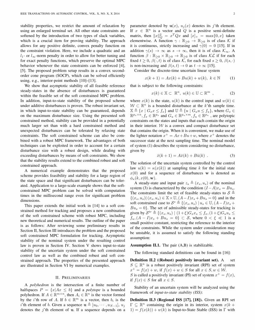
The modifications introduced in Problem PsN (x, zr) are ex-plained in the following sections and are illustrated in Figure 1.

IEEE TRANSACTIONS ON AUTOMATIC CONTROL, VOL. ?, NO. ?, ? 201? 1

Soft Constrained Model Predictive Control withRobust Stability Guarantees

Melanie N. Zeilinger, Member, IEEE, Manfred Morari, Fellow, IEEE, and Colin N. Jones, Member, IEEE

Abstract

Index Terms

Soft constraints, Model Predictive Control

!!s

!!1

!!2

!!3 = 0 Cs

f

X

EsT (x!

s , u!s)

x!0 = x

x!1

x!2

x!3

!!0

Esf (x!

N , x!s)

M.N. Zeilinger is with the Department of Electrical Engineering and Computer Sciences, UC Berkeley, CA 94702, USA, and the Department of EmpiricalInference, Max Planck Institute for Intelligent Systems, 72076 Tübingen, Germany, email: [email protected].

C.N. Jones is with the Laboratoire d’Automatique, École Polytechnique Fédérale de Lausanne (EPFL), CH – 1015 Lausanne, Switzerland, email:[email protected].

M. Morari is with the Automatic Control Laboratory, ETH Zurich, CH – 8092 Zurich, Switzerland, email: [email protected] received May 21, 2013; revised December 2, 2013.

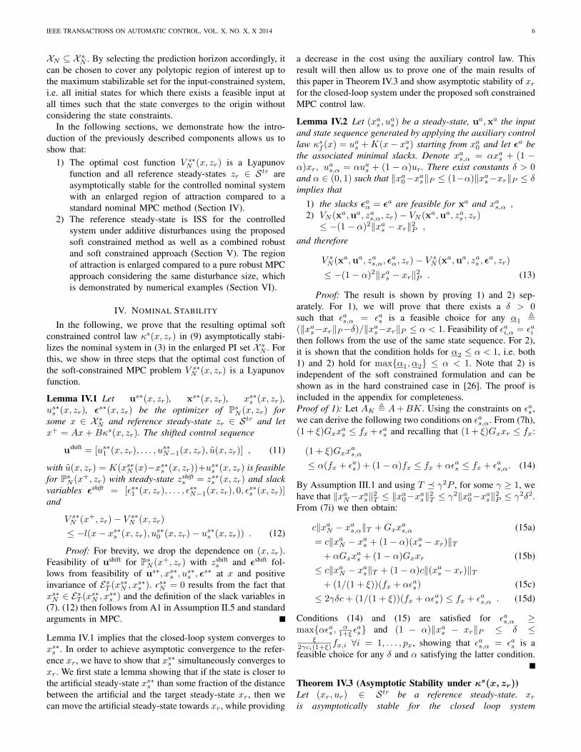
Fig. 1. Illustration of the optimal slack variables ε∗s , ε∗i , i = 0, 1, 2, 3, theterminal set Esf (x∗s , u

∗s), the scaled terminal set EsT (x∗N , x

∗s) and enlarged

terminal set Csf for an initial state x outside X.

Problem PsN (x, zr) implicitly defines the set of feasible con-trol sequences UsN (x, zs) = u | ∃ x s.t. (7b)− (7d), (7f) holdand feasible initial states X sN , x | ∃zs ∈ Ss s.t. UsN (x, zs) 6=∅. For a given state x ∈ X sN and reference zr ∈ Str, ProblemPsN (x, zr) results in a convex second order cone program(SOCP) and its solution yields the optimal control sequenceus∗(x, zr). Note that SOCPs can be efficiently solved using,e.g., interior-point methods [10]–[13]. The implicit optimalsoft constrained MPC control law is then given in a recedinghorizon fashion by

κs(x, zr) , us∗0 (x, zr) . (9)

1) Relaxation of the Terminal Constraint: The terminal setfor tracking in (7f) is relaxed by two effects: i) by allowing theartificial set point to move to any steady-state (xs, us) ∈ Sssatisfying only the input constraints, ii) by allowing the stateconstraints to be violated in the terminal set Esf (xs, us). Thisresults in an enlarged terminal set Csf , x | ∃ (xs, us) ∈Ss s.t. x ∈ Esf (xs, us) for the MPC problem, given by theset of all states x, for which there exists a steady-state suchthat the terminal constraint is satisfied.

Assumption III.1. For any given (xs, us) ∈ Ss, Esf (xs, us) isa PI set under the local control law κsf (x) = K(x− xs) + ussatisfying the following conditions:A3: κsf (x) ∈ U ∀x ∈ Esf (xs, us)A4: ‖Ax+Bκsf (x)− xs‖2T = ‖(A+BK)(x− xs)‖2T

≤ ‖x− xs‖2T .

It is further assumed that the set Csf is compact.

Note that compared to condition A2 in Assumption II.5,condition A3 only enforces the input constraints. ConditionA4 is slightly stronger than set invariance and is requiredfor proving stability in Section IV. If K is taken as theinfinite horizon LQR control law, which is a common choicein MPC, a matrix T satisfying condition A4 is, e.g., givenby the solution to the discrete-time algebraic Riccati equation.Compactness of Csf is required to ensure boundedness of the


feasible set and in turn uniform continuity of the optimal valuefunction V s∗N (x, zr) (Lemma V.1). It can be easily satisfied byimposing a large upper bound on the steady-state xs.

Lemma III.2 A matrix T and function r defining the invariantellipsoidal target set Esf (xs, us) in (8) such that Assump-tion III.1 is satisfied can be computed by solving a convexlinear matrix inequality (LMI).

Proof: See appendix.

Remark III.3. The amount, by which the terminal set can beenlarged depends on Ss. An increase can only be achieved ifthe reference steady-state is not the only steady-state, i.e xscan differ from xr, and the imposed hard constraints are notlimiting the size of the terminal set to be always contained inthe state constraints.

Remark III.4. The combination of moving the artificialsteady-state and neglecting state constraints offers a significantincrease of the terminal set, which is the reason for choosingthe tracking formulation [9]. The proposed scheme could alsobe applied to a standard MPC formulation by allowing stateconstraints to be violated in the terminal set, which would,however, result in a smaller terminal and hence feasible set.

2) Slack Variables: We now explain the crucial item in theproposed soft constrained scheme, the slack variables εs andεi that are used to soften all state constraints:• εs represents the amount of constraint relaxation that is

necessary in order to include the ellipsoid EsT (xN , xs)for a particular value of (xs, us) into the relaxed stateconstraints, where

EsT (xN , xs) ,x∣∣∣ ‖x− xs‖2T ≤ ‖xN − xs‖2T (10)

is a scaling of the ellipsoidal terminal set Esf (xs, us)containing xN on its boundary. This can be expressedas

maxx

Gx,ix

∣∣∣‖x− xs‖2T ≤ ‖xN − xs‖2T ≤ fx,i + εs,i

∀i = 1, . . . , px, resulting in the following condition [24]:

‖T− 12GTx,i‖2‖T

12 (xN − xs)‖2 ≤ fx,i + εs,i −Gx,ixs

∀i = 1, . . . , px, which corresponds to (7i) with ci =‖T− 1

2GTx,i‖2 ∀i = 1, . . . , px and is a collection of pxconvex second order cone constraints.

• εi in (7e) represents the additional constraint violation ofeach state xi for i = 0, . . . , N − 1 with respect to thestate constraints relaxed by εs.

The use of the slack variable εs defined by (7i) ensures that theterminal state, which is contained in EsT (xN , xs), will lie insidethe state constraints relaxed by the amount εs and will notrequire a further relaxation of the state constraints, i.e. εN = 0,where εN is the slack variable of the terminal state defined byGxxN ≤ fx+ εs+ εN . This provides feasibility of the shiftedsequence using the shifted slack variables with the last slackvariable being zero. Constraint (7h) additionally enforces thatthe steady-state xs always has to lie in the interior of theconstraints relaxed by εs by an amount ξ, which is a user-specified small, positive parameter. For a state that is close to

the artificial steady-state, this ensures that the steady-state canalways be shifted towards the reference without increasing theslack variables.

As will be shown in Section IV, these items provide thatthe optimal cost function is still a Lyapunov function andare hence crucial for proving stability of the proposed softconstrained MPC scheme.

Remark III.5. By Assumption III.1, the set EsT (xN , xs) is apositively invariant set under the local control law κsf (x).

Remark III.6. Defining εs by the inclusion of Esf (xs, us) intothe relaxed state constraints would also provide εN = 0 andwould allow for proving asymptotic stability. We have chosenEsT (xN , xs) here, since it results in a slack closer to the actualconstraint violation of the terminal state.

Remark III.7. While a strictly positive value of ξ in con-straint (7h) is required to prove stability of the closed-loopsystem (Lemma IV.2), the particular choice is not crucial andfor ξ 1, it will have a negligible or no effect on the systembehavior.

Remark III.8 (Hard state constraints). For ease of nota-tion, we assume the relaxation of all state constraints exceptthe terminal constraint in PsN (x, zr). However, the resultsdirectly extend to the case where some of the state constraintsare considered as hard constraints with only minor notationalchanges.

3) Penalty Functions: A penalty function on the slackvariables is included in the cost in (7a), in order to minimizethe constraint violation and to ensure satisfaction of the stateconstraints whenever possible. The penalty can be chosenas in standard soft constrained schemes. In the proposedformulation, we include a quadratic penalty, which is oftenpreferable for tuning the constraint violation [4], and an l1 orl∞-norm penalty, in order to allow for exact penalty functions.It is well-known that, when the weights on the l1 or l∞-normsare sufficiently large and there exists a feasible solution to thehard constrained problem PN (x, zr), then the optimal solutionto the soft constrained problem PsN (x, zr) corresponds to thatof the hard constrained problem [5], [6], [25]. Note that anl1 or l∞-norm is also used in the offset cost for penalizingthe deviation of the artificial from the reference steady-state,in order to enforce the reference as the target point if it isfeasible [22].

Remark III.9. The results presented in this paper hold forany positive definite, convex penalty function on the slackvariables, i.e. the quadratic penalty could also be omitted. Notethat the linear penalties can be simplified for implementation.The l1-norm can directly be replaced with the sum of the slackvariables, and the l∞-norm can be formulated by using a singleslack variable for the constraint relaxation at each stage thatis then penalized in the cost.

C. Soft Constrained MPC Properties

The soft constrained formulation PsN (x, zr) enlarges thefeasible set compared to the hard constrained problem since


XN ⊆ X sN . By selecting the prediction horizon accordingly, itcan be chosen to cover any polytopic region of interest up tothe maximum stabilizable set for the input-constrained system,i.e. all initial states for which there exists a feasible input atall times such that the state converges to the origin withoutconsidering the state constraints.

In the following sections, we demonstrate how the intro-duction of the previously described components allows us toshow that:

1) The optimal cost function V s∗N (x, zr) is a Lyapunovfunction and all reference steady-states zr ∈ Str areasymptotically stable for the controlled nominal systemwith an enlarged region of attraction compared to astandard nominal MPC method (Section IV).

2) The reference steady-state is ISS for the controlledsystem under additive disturbances using the proposedsoft constrained method as well as a combined robustand soft constrained approach (Section V). The regionof attraction is enlarged compared to a pure robust MPCapproach considering the same disturbance size, whichis demonstrated by numerical examples (Section VI).

IV. NOMINAL STABILITY

In the following, we prove that the resulting optimal softconstrained control law κs(x, zr) in (9) asymptotically stabi-lizes the nominal system in (3) in the enlarged PI set X sN . Forthis, we show in three steps that the optimal cost function ofthe soft-constrained MPC problem V s∗N (x, zr) is a Lyapunovfunction.

Lemma IV.1 Let us∗(x, zr), xs∗(x, zr), xs∗s (x, zr),us∗s (x, zr), εs∗(x, zr) be the optimizer of PsN (x, zr) forsome x ∈ X sN and reference steady-state zr ∈ Str and letx+ = Ax+Bκs(x, zr). The shifted control sequence

ushift = [us∗1 (x, zr), . . . , us∗N−1(x, zr), u(x, zr)] , (11)

with u(x, zr) = K(xs∗N (x)−xs∗s (x, zr))+us∗s (x, zr) is feasiblefor PsN (x+, zr) with steady-state zshift

s = zs∗s (x, zr) and slackvariables εshift = [εs∗1 (x, zr), . . . , ε

s∗N−1(x, zr), 0, ε

s∗s (x, zr)]

and

V s∗N (x+, zr)− V s∗N (x, zr)

≤ −l(x− xs∗s (x, zr), us∗0 (x, zr)− us∗s (x, zr)) . (12)

Proof: For brevity, we drop the dependence on (x, zr).Feasibility of ushift for PsN (x+, zr) with zshift

s and εshift fol-lows from feasibility of us∗, xs∗s , u

s∗s , ε

s∗ at x and positiveinvariance of EsT (xs∗N , x

s∗s ). εs∗N = 0 results from the fact that

xs∗N ∈ EsT (xs∗N , xs∗s ) and the definition of the slack variables in

(7). (12) then follows from A1 in Assumption II.5 and standardarguments in MPC.

Lemma IV.1 implies that the closed-loop system converges toxs∗s . In order to achieve asymptotic convergence to the refer-ence xr, we have to show that xs∗s simultaneously converges toxr. We first state a lemma showing that if the state is closer tothe artificial steady-state xs∗s than some fraction of the distancebetween the artificial and the target steady-state xr, then wecan move the artificial steady-state towards xr, while providing

a decrease in the cost using the auxiliary control law. Thisresult will then allow us to prove one of the main results ofthis paper in Theorem IV.3 and show asymptotic stability of xrfor the closed-loop system under the proposed soft constrainedMPC control law.

Lemma IV.2 Let (xas , uas) be a steady-state, ua,xa the input

and state sequence generated by applying the auxiliary controllaw κsf (x) = uas +K(x− xas) starting from xa0 and let εa bethe associated minimal slacks. Denote xas,α = αxas + (1 −α)xr, u

as,α = αuas + (1 − α)ur. There exist constants δ > 0

and α ∈ (0, 1) such that ‖xa0−xas‖P ≤ (1−α)‖xas−xr‖P ≤ δimplies that

1) the slacks εaα = εa are feasible for xa and xas,α ,2) VN (xa,ua, zas,α, zr)− VN (xa,ua, zas , zr)≤ −(1− α)2‖xas − xr‖2P ,

and therefore

V sN (xa,ua, zas,α, εaα, zr)− V sN (xa,ua, zas , ε

a, zr)

≤ −(1− α)2‖xas − xr‖2P . (13)

Proof: The result is shown by proving 1) and 2) sep-arately. For 1), we will prove that there exists a δ > 0such that εas,α = εas is a feasible choice for any α1 ,(‖xas−xr‖P−δ)/‖xas−xr‖P ≤ α < 1. Feasibility of εai,α = εaithen follows from the use of the same state sequence. For 2),it is shown that the condition holds for α2 ≤ α < 1, i.e. both1) and 2) hold for maxα1, α2 ≤ α < 1. Note that 2) isindependent of the soft constrained formulation and can beshown as in the hard constrained case in [26]. The proof isincluded in the appendix for completeness.Proof of 1): Let AK , A+BK. Using the constraints on εas ,we can derive the following two conditions on εas,α. From (7h),(1 + ξ)Gxx

as ≤ fx + εas and recalling that (1 + ξ)Gxxr ≤ fx:

(1 + ξ)Gxxas,α

≤ α(fx + εas) + (1− α)fx ≤ fx + αεas ≤ fx + εas,α. (14)

By Assumption III.1 and using T γ2P , for some γ ≥ 1, wehave that ‖xaN−xas‖2T ≤ ‖xa0−xas‖2T ≤ γ2‖xa0−xas‖2P ≤ γ2δ2.From (7i) we then obtain:

c‖xaN − xas,α‖T +Gxxas,α (15a)

= c‖xaN − xas + (1− α)(xas − xr)‖T+ αGxx

as + (1− α)Gxxr (15b)

≤ c‖xaN − xas‖T + (1− α)c‖(xas − xr)‖T+ (1/(1 + ξ))(fx + αεas) (15c)≤ 2γδc+ (1/(1 + ξ))(fx + αεas) ≤ fx + εas,α . (15d)

Conditions (14) and (15) are satisfied for εas,α ≥maxαεas , α

1+ξ εas and (1 − α)‖xas − xr‖P ≤ δ ≤

ξ2γci(1+ξ)fx,i ∀i = 1, . . . , px, showing that εas,α = εas is afeasible choice for any δ and α satisfying the latter condition.

Theorem IV.3 (Asymptotic Stability under κs(x, zr))Let (xr, ur) ∈ Str be a reference steady-state. xris asymptotically stable for the closed loop system


x(k + 1) = Ax(k) + Bκs(x(k), zr) with region of attractionX sN .

Proof: Using Lemma IV.1 and IV.2, it can be shownthat V s∗N (x, zr) is a Lyapunov function by following the samearguments as in the hard constrained case presented in [26].The proof is included in the appendix.

V. ROBUST STABILITY

In practice, model uncertainties or external disturbancescause a deviation from the nominal system dynamics in (3).There are two general approaches to deal with disturbances. Inthe case of linear systems and under certain assumptions on theMPC problem setup, the nominal control law offers inherentrobust stability properties [19], [27] and robust stability canbe guaranteed in an RPI set that depends on the considereddisturbance size. Robust MPC schemes, on the other hand,take a worst-case disturbance size explicitly into account bychanging the problem formulation and/or tightening the con-straints, e.g. using a min-max or a tube-based MPC approach(see e.g. [1], [19], [20], [28] and the references therein).

In a hard constrained setup, both techniques have potentiallimitations. Using a nominal MPC scheme, the RPI set, inwhich stability can be guaranteed, may be prohibitively smallfor the considered disturbance size. Using a robust MPCscheme, the choice of the disturbance bound employed in thecontroller design is often conservative, since feasibility of theMPC problem may be lost if the disturbance exceeds the pre-defined bound.

The proposed soft constrained scheme can be used toimprove the properties of both techniques. The nominal softconstrained method offers inherent robust stability propertiesand can thereby provide stability in a potentially much largerRPI set, since state constraints can be relaxed. It is impor-tant to note that, while stability is formally only guaranteedwithin the RPI set, the control law is defined everywherein the enlarged feasible set. If constraint satisfaction shouldbe guaranteed for a certain expected size of the disturbance,the soft constrained scheme can be combined with a robustMPC approach. While the robust method designs the problemfor a certain disturbance bound, the use of the proposedsoft constrained formulation ensures feasibility and stabilityof the MPC problem if the disturbance exceeds this bound.Conservatism in the choice of the disturbance bound for robustMPC can thereby be avoided and the system performanceimproved.

Robust stability under both the nominal soft constrainedMPC scheme as well as the combination with a robust MPCapproach is proven in the following using the framework ofinput-to-state stability.

A. ISS of Nominal Soft Constrained MPC

Assume that the system is subject to an additive uncertaintyas given in (1). Because of the disturbance, the shifted se-quence ushift in (11) may no longer be feasible for PsN (x+, zr).For all x+ ∈ X sN there does, however, exist a feasible solutionto PsN (x+, zr) and input-to-state stability can be shown in

an RPI set X sW ⊂ X sN . It is given by the maximum robustpositively invariant set for the controlled uncertain systemx+ = Ax+Bκs(x, zr)+w under the optimal soft constrainedMPC control law in (9). We make use of the following resultin order to show that the uncertain system in (1) under thenominal control law κs(x, zr) is input-to-state stable withrespect to the (unspecified) disturbance setW in Theorem V.2.

Lemma V.1 (Continuity of V s∗N (x)) Consider problemPsN (x, zr). The optimal value function V s∗N (x, zr) isuniformly continuous in x on X sN .

Proof: Continuity follows directly from continuity andconvexity of the cost function and the constraints in (7) as wellas compactness of the constraint set for all x ∈ X sN (Theorem4.3.3 in [29]), where the latter is provided by the fact that theterminal set is compact (Assumption III.1). Uniform continuitythen follows, since X sN is compact (e.g. Proposition 5 in [20]).

Theorem V.2 (ISS under κs(x, zr)) Let (xr, ur) ∈ Str bea given reference steady-state. xr is ISS for the closed loopsystem x(k+1) = Ax(k)+Bκs(x(k), zr)+w(k) with respectto w(k) ∈ W with region of attraction X sW .

Proof: From the proof of Theorem IV.3 and Lemma V.1it follows that V s∗N (x, zr) is a uniformly continuous Lyapunovfunction and hence there exists a K-class function γ(·), suchthat |V s∗N (y, zr) − V s∗N (x, zr)| ≤ γ(‖y − x‖) (see, e.g.,[20], A.11) as well as a K∞-class function α3(·) such thatV s∗N (Ax+Bκs(x, zr), zr)− V s∗N (x, zr) ≤ −α3(‖x− xr‖). Itfollows from these facts that

V s∗N (x+, zr)− V s∗N (x, zr)

= V s∗N (Ax+Bκs(x, zr) + w, zr)− V s∗N (x, zr)

+ V s∗N (Ax+Bκs(x, zr), zr)− V s∗N (Ax+Bκs(x, zr), zr)

≤ −α3(‖x− xr‖) + γ(‖w‖) ,

i.e. V s∗N (x, zr) is an ISS-Lyapunov function with respect tow ∈ W and xr is ISS for the closed-loop system.

The uncertain system controlled by the soft constrained controllaw κs(x, zr) is hence input-to-state stable against sufficientlysmall disturbances. Since the RPI set X sW depends on W ,the size of the disturbances and the corresponding region, forwhich stability can be formally guaranteed, depend on theparticular system of interest.

In the following section we will show that the previouslypresented results can be directly extended to the combinationof a robust and soft constrained MPC framework, in order totake advantage of both properties.

B. Combination of Robust and Soft Constrained MPC

We assume in the following that the system is affected bytwo uncertainties:

x(k + 1) = Ax(k) +Bu(k) + w1(k) + w2(k) , (16)

where w1 ∈ W1, w2 ∈ W2 and W1,W2 are convex andcompact sets that each contain the origin. The disturbancew1 is explicitly taken into account by using a robust MPC


technique, which provides constraint satisfaction and stabilityin the presence of w1. Feasibility and stability in the presenceof w2 is guaranteed by means of the proposed soft constrainedscheme.

In this work, we apply the tube-based robust MPC approachfor linear systems [28]. The method is based on the use of afeedback policy of the form u = u + K(x − x) that boundsthe effect of the disturbance w1 and keeps the states x of theuncertain system under w1 close to the states of the nominalsystem in (3). The use of tightened state and input constraintsensures feasibility of the uncertain system in (16) despitethe disturbance w1: X = X Z ,

x | Gxx ≤ fx

, U =

UKZ ,u | Guu ≤ fu

, with fx,i = fx,i−hZ(GTx,i), i =

1, . . . , px, fu,i = fu,i − hZ(KTGTu,i), i = 1, . . . , pu, where Zis an RPI set for the controlled system x+ = (A+BK)x+w1

and hZ(a) = supx∈Z aTx is the support function of Z eval-

uated at a. Note that the tightened state and input constraintsagain result in compact polytopes. See [28] for a detaileddescription of the method. The tracking approach described inSection II was extended to a robust tube-based MPC methodfor tracking in [23], which will be combined in the followingwith the soft constrained scheme proposed in Section III.

Problem PrsN (x, zr) (Robust soft constrained MPC problem)

V rs∗N (x, zr) = minx,u,zs,ε,zr

V sN (x, u, zs, ε, zr) + Vf (x− x0)

s.t. x ∈ x0 ⊕Z ,

(7c)− (7j) ,

where in the constraints (7c)-(7j), fx, fu and Esf (xs, us) are re-placed with fx, fu and Esf (xs, us), respectively. The conditionson the robust terminal set for tracking Esf (xs, us) are obtainedby replacing the input constraints U in Assumption III.1 withU. Compared to [28], we propose to augment the cost withthe term Vf (x − x0), which offers the advantage of directlyproviding an ISS Lyapunov function (Theorem V.4, see also[26], [30] for more details).

Remark V.3. The use of tightened state constraints in the softconstrained formulation, i.e. replacing fx with fx, has theadvantage that the behavior of the robust MPC controller isrecovered if the constraints can be enforced. Stability would,however, also be provided by using fx.

The set of feasible initial states of the robust soft constrainedproblem is denoted by X rsN . The robust formulation does notchange the problem structure and Problem PrsN (x, zr) againresults in a convex SOCP. For a given state x ∈ X rsN , thesolution of PrsN (x, zr) yields the optimal control sequenceurs∗(x, zr) and the optimal first tube center xrs∗0 (x, zr). Therobust soft constrained control law is then given in a recedinghorizon fashion by

κrs(x, zr) , urs∗0 (x, zr) +K(x− xrs∗0 (x, zr)) . (17)

Input-to-state stability will in the following be shown for therobust invariant set X rsW ⊆ X rsN , given by the maximum robustpositively invariant set for the controlled uncertain systemx+ = Ax+Bκrs(x, zr) +w1 +w2 with w1 ∈ W1, w2 ∈ W2.

Let Str , (xs, us) ∈ Str | (1+ξ)Gxxs ≤ fx, (1+ξ)Guus ≤fu.Theorem V.4 (ISS under κrs(x, zr)) Let (xr, ur) ∈ Strbe a given reference steady-state. xr is ISS for the closed loopsystem x(k+ 1) = Ax(k) +Bκrs(x(k), zr) +w1(k) +w2(k)with respect to w1(k) ∈ W1 and w2(k) ∈ W2 with region ofattraction X rsW .

Proof: The first part of the proof assumes w2 = 0 and fol-lows similar steps as in Section IV to show that V rs∗N (x, zr) isan ISS Lyapunov function with respect to w1. A more detailedversion of this part of the proof can also be found in [26]. Thesecond part of the proof then shows that V rs∗N (x, zr) is also anISS Lyapunov function with respect to w2. In the following,we omit the dependence of the optimal solution on (x, zr). Letw2 = 0, i.e. x+ = Ax+Bκrs(x, zr)+w1. Lemma IV.1 extendsto the robust problem setup showing feasibility of the shiftedsequence with εshift = [εrs∗1 , . . . , εrs∗N−1, 0, ε

rs∗s ]. Using uniform

continuity of Vf (·), x+ = xrs∗1 +(A+BK)(x−xrs∗0 )+w1 andAssumption II.5, it can be shown that there exists a K-classfunction γ1(·) such that Vf (x+ − xrs∗1 ) − Vf (x − xrs∗0 ) ≤−‖x − xrs∗0 ‖2Q + γ1(‖w1‖). Using standard arguments andconvexity of ‖ · ‖2Q, it then follows that

V rs∗N (Ax+Bκrs(x, zr) + w1, zr)− V rs∗N (x, zr)

≤ V sN (xshift, ushift, zrs∗s , εshift, zr) + Vf (x+ − xrs∗1 )

− V sN (xrs∗, urs∗, zrs∗s , εrs∗, zr)− Vf (x− xrs∗0 )

≤ −‖xrs∗0 − xrs∗s ‖2Q − ‖x− xrs∗0 ‖2Q + γ1(‖w1‖)

≤ −1

2‖x− xrs∗s ‖2Q + γ1(‖w1‖) . (18)

Following similar arguments as in the proof of Theorem IV.3and using optimality of V rs∗N (x, zr) it can be shown that thereexist K∞-class functions α(·), α(·) such that V rs∗N (x, zr) ≥α(‖x− xr‖) ∀x ∈ X rsN and V rs∗N (x, zr) ≤ α(‖x− xr‖) ∀x ∈Esf (xr, ur) ⊕ Z . The condition that remains to be shown isthat (18) also provides a strict decrease that is a function of‖x−xr‖2Q. Lemma IV.2 directly extends to the robust problemformulation by replacing the constraints with the tightenedform (Part 1)) and since the additional cost term Vf (x− x0)does not contain the steady-state xs and is irrelevant for theargument (Part 2)). Considering the same cases and argumentsas in the proof of Theorem IV.3, it can then be shown that thereexists a K∞-class function α3(·) such that

V rs∗N (Ax+Bκrs(x, zr) + w1, zr)− V rs∗N (x, zr)

≤ −α3(‖x− xr‖) + γ1(‖w1‖) .

For the second part of the proof, uniform continuity of the op-timal value function V rs∗N (x, zr) follows as in the non-robustcase from the proof of Lemma V.1. Therefore, there existsa K-class function γ2(·), such that |V rs∗N (y) − V rs∗N (x)| ≤γ2(‖y − x‖) and we obtain

V rs∗N (Ax+Bκrs(x, zr) + w1 + w2, zr)− V rs∗N (x, zr)

≤ −α3(‖x− xr‖) + γ1(‖w1‖) + γ2(‖w2‖) ,

proving the result.Theorem V.4 proves ISS of the uncertain system in (16) con-trolled by κrs(x, zr) in (17) with respect to the disturbances


w1 ∈ W1 and w2 ∈ W2 and shows that the results presentedfor the soft constrained MPC method can directly be extendedto the combination of a robust and soft constrained approach.

VI. NUMERICAL EXAMPLES

In this section, the proposed methods for soft constrainedand robust soft constrained MPC are illustrated for a small-scale example and computation times for a large-scale problemare provided. All set computations were carried out usingYALMIP [31] and the MPT toolbox [32].

A. Illustrative Example

Consider the following unstable system:

x(k + 1) =

[1.05 1

0 1

]x(k) +

[1

0.5

]u(k) + w(k) . (19)

The prediction horizon was chosen to be N = 5, theconstraints on the states and control inputs to ‖x‖∞ ≤ 5and ‖u‖∞ ≤ 1, Q = I , R = 1 and S = 100I . Theterminal cost function Vf (·) is taken as the unconstrainedinfinite horizon optimal value function for the nominal systemwith P = [ 1.9119 0.2499

0.2499 2.6510 ] and κf (x) = K(x − xs) + us isthe corresponding optimal LQR controller. The exact penaltymultipliers were chosen as ρε = ρx = ρu = 100, which wasobserved to provide optimality in XN . For simplicity, we takexr = 0, ur = 0 as the reference steady-state for the followingillustrations.

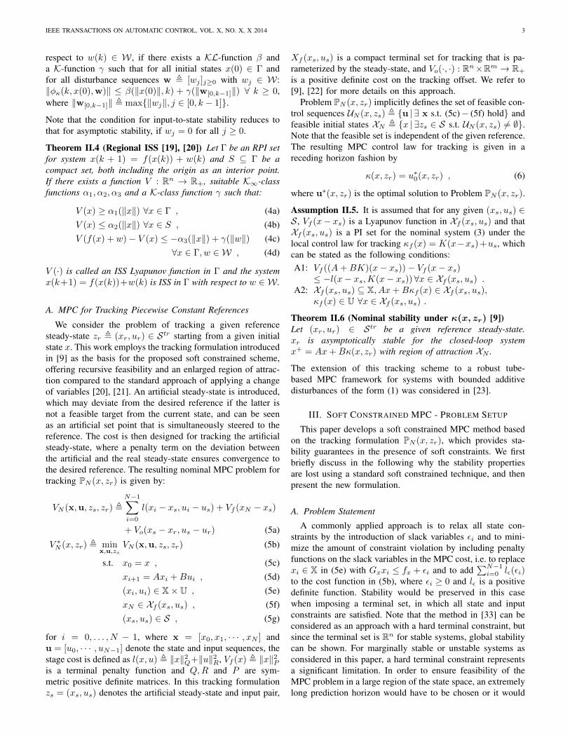
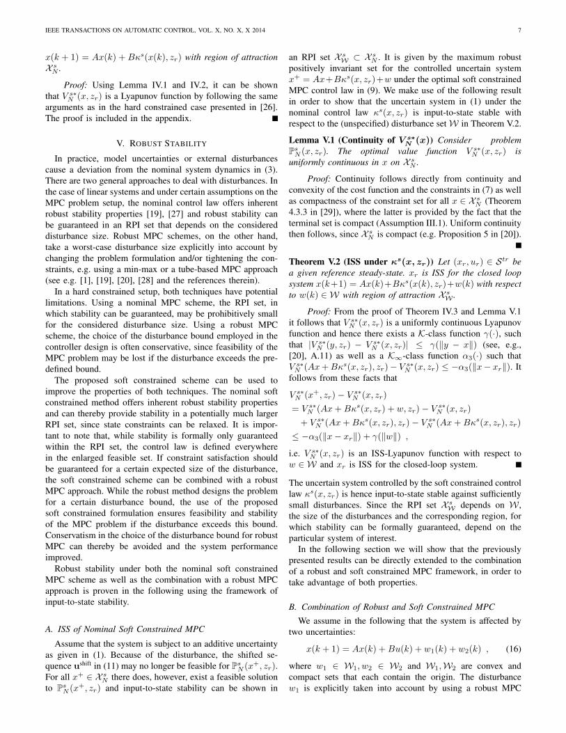
1) Soft Constrained MPC: The feasible set X s5 and theenlarged terminal set Csf for the soft constrained approachPsN (x, zr) are illustrated and compared with the feasible set X5

and terminal set Cf for the hard constrained problem PN (x, zr)in Figure 2, which demonstrates that the soft constrainedapproach significantly enlarges the feasible set and therebythe region of attraction for the nominal closed-loop system.This shows that the proposed method provides the benefitsof soft constraints and ensures feasibility of the optimizationproblem in a large region while still guaranteeing stability ofthe closed-loop system.

−30 −20 −10 0 10 20 30

−5

−4

−3

−2

−1

0

1

2

3

4

5

x1

x 2

X

X s5

X5

Cf

Csf

Fig. 2. Feasible and terminal set for the soft constrained problem PsN (x, zr)

for N = 5 in comparison with the feasible and terminal set of the hardconstrained problem PN (x, zr).

−30 −20 −10 0 10 20 30

−5

−4

−3

−2

−1

0

1

2

3

4

5

x1

x 2

X5

X s5

X sW0.25

X sW0.15

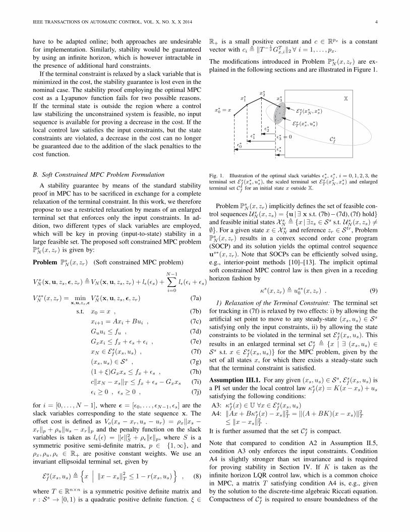
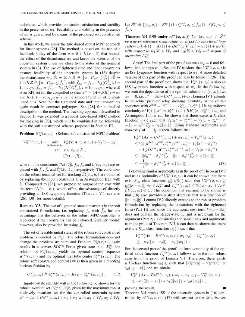
Fig. 3. Feasible set and RPI sets of PsN (x, zr) for w ∈ 0.15, 0.25 together

with a closed-loop trajectory starting at x(0) = [20, 1.25]T under a sequenceof extreme disturbances. Dots represent the optimal steady-state xs∗s (x(k), 0)at each sampling time.

−30 −20 −10 0 10 20 30

−5

−4

−3

−2

−1

0

1

2

3

4

5

x1

x 2

X sW0.25

X s5

X rs5

X rsW0.25

X5

X rh5

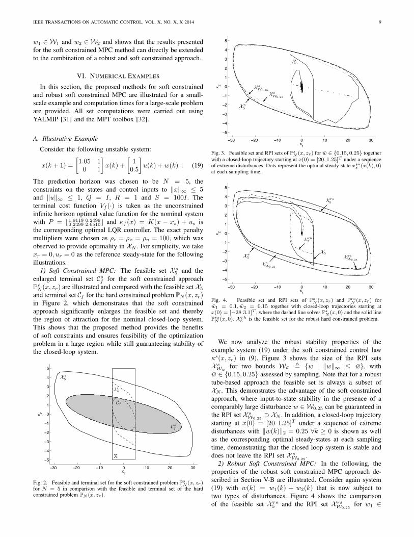
Fig. 4. Feasible set and RPI sets of PsN (x, zr) and Prs

N (x, zr) forw1 = 0.1, w2 = 0.15 together with closed-loop trajectories starting atx(0) = [−28 3.1]T , where the dashed line solves Ps

N (x, 0) and the solid linePrsN (x, 0). X rh

5 is the feasible set for the robust hard constrained problem.

We now analyze the robust stability properties of theexample system (19) under the soft constrained control lawκs(x, zr) in (9). Figure 3 shows the size of the RPI setsX sWw

for two bounds Ww , w | ‖w‖∞ ≤ w, withw ∈ 0.15, 0.25 assessed by sampling. Note that for a robusttube-based approach the feasible set is always a subset ofXN . This demonstrates the advantage of the soft constrainedapproach, where input-to-state stability in the presence of acomparably large disturbance w ∈ W0.25 can be guaranteed inthe RPI set X sW0.25

⊃ XN . In addition, a closed-loop trajectorystarting at x(0) = [20 1.25]T under a sequence of extremedisturbances with ‖w(k)‖2 = 0.25 ∀k ≥ 0 is shown as wellas the corresponding optimal steady-states at each samplingtime, demonstrating that the closed-loop system is stable anddoes not leave the RPI set X sW0.25

.2) Robust Soft Constrained MPC: In the following, the

properties of the robust soft constrained MPC approach de-scribed in Section V-B are illustrated. Consider again system(19) with w(k) = w1(k) + w2(k) that is now subject totwo types of disturbances. Figure 4 shows the comparisonof the feasible set X rs5 and the RPI set X rsW0.25

for w1 ∈


Ww1, w2 ∈ Ww2

with w1 = 0.1, w2 = 0.15 in comparisonwith the feasible set X s5 and the RPI set X sW0.25

of the pure softconstrained approach. The feasible set of the hard constrainedrobust MPC problem, i.e. Problem PrsN (x, zr) with (xs, us) ∈S, εs = 0, εi = 0, w = w1 + w2 ∈ W0.25 is denoted byX rh5 . Due to the tightening of the input constraints, the robustsoft constrained approach has a smaller feasible set whencompared to the pure soft constrained method. However, incomparison with the hard constrained robust MPC method, thefeasible set for the combined approach is significantly larger,while still guaranteeing ISS with respect to w1 in X rs5 . TheRPI set X rsW0.25

is only slightly smaller than X rs5 and input-to-state stability with respect to the combined disturbancew = w1 + w2 ∈ W0.25 is provided in a comparably largeset. Closed-loop trajectories starting from x(0) = [−28 3.1]T

are shown for both the robust soft constrained and the puresoft constrained approach under a sequence of extreme distur-bances ‖w1(k)‖2 = 0.1 and a disturbance ‖w2(k)‖2 ∈ W0.15

∀k ≥ 0 that additionally affects the system at every thirdsampling time. Figure 4 demonstrates that both approachesprovide input-to-state stability of the closed-loop system. Therobust soft constrained approach steers the system earlier to-wards the origin and the trajectory remains in X rsW0.25

, since therobust formulation is designed to counteract the disturbancew1. The soft constrained approach allows for a larger deviationof the state within the RPI set X sW0.25

. This shows that byusing a combination of a robust and soft constrained method,robustness against a certain disturbance size can be providedwhile ensuring stability if the disturbance exceeds this bound.

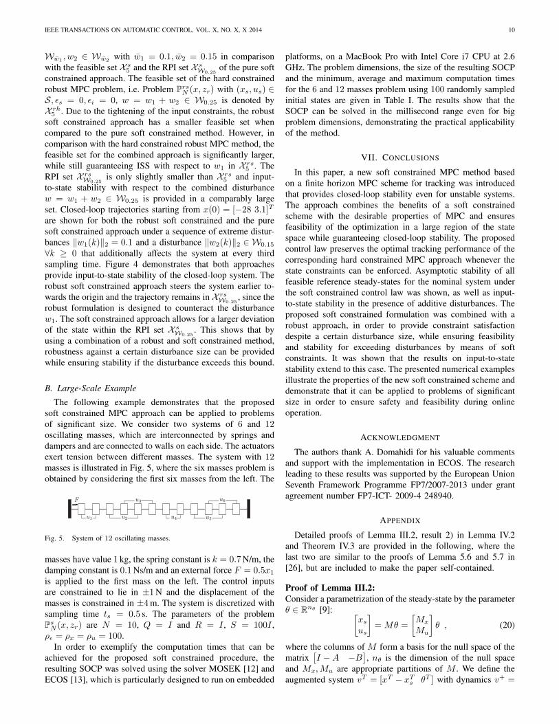
B. Large-Scale Example

The following example demonstrates that the proposedsoft constrained MPC approach can be applied to problemsof significant size. We consider two systems of 6 and 12oscillating masses, which are interconnected by springs anddampers and are connected to walls on each side. The actuatorsexert tension between different masses. The system with 12masses is illustrated in Fig. 5, where the six masses problem isobtained by considering the first six masses from the left. The

136 9 Soft Constrained MPC with Robust Stability Guarantees

Robust Soft Constrained MPC

In the following the properties of the robust soft constrained MPC approach described inSection 9.7 are illustrated. Consider again system (9.17) with w(k) = w1(k)+w2(k) thatis now subject to two types of disturbances. Figure 9.5(b) shows the comparison of thefeasible set X rs

5 and the RPI set X rsW0.2

for w1 ! Ww1 , w2 ! Ww2 with w1 = 0.1, w2 = 0.1

in comparison with the feasible set X sN and the RPI set X s

W0.2of the pure soft constrained

approach. The feasible set of the hard constrained robust MPC problem, i.e. ProblemPrs

N (x) with xs = us = 0, !s = 0, !i = 0, w = w1 + w2 ! W0.2 is denoted by X rh5 . Due

to the tightening of the input constraints, the robust soft constrained approach has asignificantly smaller feasible set when compared to the pure soft constrained method.However, in comparison with the hard constrained robust MPC method, the feasibleset for the combined approach is significantly larger while still guaranteeing ISS withrespect to w1 in X rs

N , which is almost as large as the nominal feasible set X5. TheRPI set X rs

W0.2is only slightly smaller than X rs

5 and input-to-state stability with respectto the combined disturbance w = w1 + w2 ! W0.2 is still provided in a comparablylarge set. Closed-loop trajectories starting from x(0) = ["9.6 1]T are shown for bothapproaches under a sequence of extreme disturbances w1(k) = ±0.1 and a disturbancew2(k) ! W0.1, k # 0, of varying size that additionally a!ects the system at every thirdsampling time. Figure 9.5(b) demonstrates that both approaches provide input-to-state stability of the closed-loop system, however the robust soft constrained approachprovides a better performance, since it is designed for the disturbance w1 that constantlya!ects the system.

9.8.2 Large-Scale Example

We now apply the soft constrained MPC approach to a large scale example and es-timate the computational e!ort required to solve the corresponding SOCP. Considerthe problem of regulating a system of 12 oscillating masses which are interconnectedby spring-damper systems and connected to walls on the side, as shown in Fig. 9.6.The six actuators exert tension between di!erent masses. The masses are 1, the spring

u1 u2

u3

u4 u5

u6F

Figure 9.6: System of oscillating masses.

constants are 1, the damping constants are 0.1 and F = 1.05x1. The state and inputconstraints are $u$! % 1, $x$! % 4, the horizon is chosen as N = 5 and the weight

Fig. 5. System of 12 oscillating masses.

masses have value 1 kg, the spring constant is k = 0.7 N/m, thedamping constant is 0.1 Ns/m and an external force F = 0.5x1

is applied to the first mass on the left. The control inputsare constrained to lie in ±1 N and the displacement of themasses is constrained in ±4 m. The system is discretized withsampling time ts = 0.5 s. The parameters of the problemPsN (x, zr) are N = 10, Q = I and R = I , S = 100I ,ρε = ρx = ρu = 100.

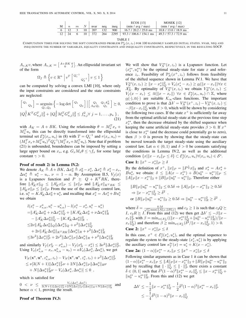
In order to exemplify the computation times that can beachieved for the proposed soft constrained procedure, theresulting SOCP was solved using the solver MOSEK [12] andECOS [13], which is particularly designed to run on embedded

platforms, on a MacBook Pro with Intel Core i7 CPU at 2.6GHz. The problem dimensions, the size of the resulting SOCPand the minimum, average and maximum computation timesfor the 6 and 12 masses problem using 100 randomly sampledinitial states are given in Table I. The results show that theSOCP can be solved in the millisecond range even for bigproblem dimensions, demonstrating the practical applicabilityof the method.

VII. CONCLUSIONS

In this paper, a new soft constrained MPC method basedon a finite horizon MPC scheme for tracking was introducedthat provides closed-loop stability even for unstable systems.The approach combines the benefits of a soft constrainedscheme with the desirable properties of MPC and ensuresfeasibility of the optimization in a large region of the statespace while guaranteeing closed-loop stability. The proposedcontrol law preserves the optimal tracking performance of thecorresponding hard constrained MPC approach whenever thestate constraints can be enforced. Asymptotic stability of allfeasible reference steady-states for the nominal system underthe soft constrained control law was shown, as well as input-to-state stability in the presence of additive disturbances. Theproposed soft constrained formulation was combined with arobust approach, in order to provide constraint satisfactiondespite a certain disturbance size, while ensuring feasibilityand stability for exceeding disturbances by means of softconstraints. It was shown that the results on input-to-statestability extend to this case. The presented numerical examplesillustrate the properties of the new soft constrained scheme anddemonstrate that it can be applied to problems of significantsize in order to ensure safety and feasibility during onlineoperation.

ACKNOWLEDGMENT

The authors thank A. Domahidi for his valuable commentsand support with the implementation in ECOS. The researchleading to these results was supported by the European UnionSeventh Framework Programme FP7/2007-2013 under grantagreement number FP7-ICT- 2009-4 248940.

APPENDIX

Detailed proofs of Lemma III.2, result 2) in Lemma IV.2and Theorem IV.3 are provided in the following, where thelast two are similar to the proofs of Lemma 5.6 and 5.7 in[26], but are included to make the paper self-contained.

Proof of Lemma III.2:Consider a parametrization of the steady-state by the parameterθ ∈ Rnθ [9]: [

xsus

]= Mθ =

[Mx

Mu

]θ , (20)

where the columns of M form a basis for the null space of thematrix

[I −A −B

], nθ is the dimension of the null space

and Mx,Mu are appropriate partitions of M . We define theaugmented system vT = [xT − xTs θT ] with dynamics v+ =


ECOS [13] MOSEK [12]M n m N nvar neq ineq (min / avg / max) (min / avg / max)6 12 3 10 207 132 900 16.7 / 20.2 / 25.0 ms 10.8 / 13.0 / 18.9 ms

12 24 6 10 372 264 2295 93.3 / 106.6 / 154.1 ms 49.3 / 57.3 / 72.9 ms

TABLE ICOMPUTATION TIMES FOR SOLVING THE SOFT CONSTRAINED PROBLEM Ps

N (x, zr) FOR 100 RANDOMLY SAMPLED INITIAL STATES. NVAR, NEQ ANDINEQ DENOTE THE NUMBER OF VARIABLES, EQUALITY CONSTRAINTS AND INEQUALITY CONSTRAINTS, RESPECTIVELY, IN THE RESULTING SOCP.

Av,Kv,where Av,K =[A+BK 0

0 I

]. An ellipsoidal invariant set

of the form

Ωf ,v ∈ Rn

∣∣∣ vT [Q−11

Q−12

]v ≤ 1

can be computed by solving a convex LMI [10], where onlythe input constraints are considered and the state constraintsare neglected:[Q1

Q2

]= argmin

Q1,Q2

− log det

[Q1

Q2

] ∣∣∣[ Q1 Q1ATK

AKQ1 Q1

] 0,

‖Q121 K

TGTu,j‖22 + ‖Q122 M

Tu G

Tu,j‖22 ≤ f2

u,j∀ j = 1, . . . , pu ,(21)

with AK = A + BK. Using the relationship θ = MTx xs +

MTu us this can be directly transformed into the ellipsoidal

terminal set Esf (xs, us) in (8) with T = Q−11 and r(xs, us) =

(MTx xs+M

Tu us)

TQ−12 (MT

x xs+MTu us). Note that if problem

(21) is unbounded, boundedness can be imposed by setting alarge upper bound on xs, e.g. GxMxθ ≤ γfx for some largeconstant γ > 0.

Proof of result 2) in Lemma IV.2:We denote AK , A+BK, ∆xa0 , xa0 −xas , ∆xas , xas −xr,∆uas , uas − ur, ν = 1 − α. By Assumption II.5, Vf (x)is a Lyapunov function and P Q + KTRK, there-fore ‖AiKx‖Q ≤ ‖AiKx‖P ≤ ‖x‖P and ‖AiKx‖KTRK ≤‖AiKx‖P ≤ ‖x‖P From the use of the auxiliary control law,i.e. uai = KAiK∆xa0 +uas , and recalling that xas = Axas +Buaswe obtain

l(xai − xas,α, uai − uas,α)− l(xai − xas , uai − uas)

=‖AiK∆xa0 + ν∆xas‖2Q + ‖KAiK∆xa0 + ν∆uas‖2R− ‖AiK∆xa0‖2Q − ‖KAiK∆xa0‖2R ,

≤2ν‖AiK∆xa0‖Q‖∆xas‖Q + ν2‖∆xas‖2Q+ 2ν‖AiK∆xa0‖KTRK‖∆uas‖R + ν2‖∆uas‖2R

≤3ν2‖∆xas‖2P + 2ν2‖∆xas‖P ‖∆uas‖R + ν2‖∆uas‖2Rand similarly Vf (xaN − xas,α)− Vf (xaN − xas) ≤ 3ν2‖∆xas‖2P .Using Vo(xas,α − xr, uas,α − ur) = αVo(∆x

as ,∆u

as), we get

VN (xa,ua, zas,α, zr)− VN (xa,ua, zas , zr) + ν2‖∆xas‖2P≤ ν[3(N + 1)‖∆xas‖2P ν + 2N‖∆xas‖P ‖∆uas‖Rν

+N‖∆uas‖2Rν − Vo(∆xas ,∆uas)] ≤ 0 ,

which is satisfied for

0 < ν ≤ Vo(∆xas ,∆uas )

3(N+1)‖∆xas‖2P+2N‖∆xas‖P ‖∆uas‖R+N‖∆uas‖2Rand

hence α < 1, proving the result.

Proof of Theorem IV.3:

We will show that V s∗N (x, zr) is a Lyapunov function. Let(xs∗s , u

s∗s ) be the optimal steady-state for state x and refer-

ence zr. Feasibility of PsN (x+, zr) follows from feasibilityof the shifted sequence shown in Lemma IV.1. We have thatV s∗N (x, zr) ≥ ‖x− x∗s‖2Q + Vo(x

∗s − xr) ≥ α(‖x− xr‖)∀x ∈

X sN . By optimality of V s∗N (x, zr) we obtain V s∗N (x, zr) ≤Vf (x − xr) ≤ α(‖x − xr‖) ∀x ∈ Esf (xr, ur) ∩ X, whereα(·), α(·) are suitable K∞-class functions. The importantcondition to prove is that ∆V = V s∗N (x+, zr)− V s∗N (x, zr) ≤−β‖x−xr‖2Q with β > 0, which will be shown by consideringthe following two cases. If the state x+ is sufficiently far awayfrom the optimal artificial steady-state at the previous time stepxs∗s , then the decrease obtained by the shifted sequence whenkeeping the same artificial steady-state provides β > 0. If x+

is close to xs∗s (and the decrease could potentially go to zero),then β > 0 is proven by showing that the steady-state canbe moved towards the target steady-state using the auxiliarycontrol law. Let α ∈ (0, 1) and δ > 0 be constants satisfyingthe conditions in Lemma IV.2, as well as the additionalcondition x|‖x− xs‖P ≤ δ ⊂ Esf (xs, us)∀(xs, us) ∈ Ss.Case 1: ‖x+ − x∗s‖P ≥ δBy the definition of x+, ‖x‖P = ‖P 1

2x‖2 and xas = Axas +Buas , we obtain: δ ≤ ‖A(x − xs∗s ) + B(us∗0 − us∗s )‖P ≤‖A‖P ‖x− xs∗s ‖2 + ‖B‖P ‖us∗0 − us∗s ‖2. Therefore either

‖B‖P ‖us∗0 − us∗s ‖2 ≤ 0.5δ ⇒ ‖A‖P ‖x− xs∗s ‖2 ≥ 0.5δ

⇒ ‖x− xs∗s ‖2Q ≥ δ2 ,

or ‖B‖P ‖us∗0 − us∗s ‖2 ≥ 0.5δ ⇒ ‖us∗0 − us∗s ‖2R ≥ δ2 ,

where δ = 0.5δ√c2 max(‖A‖P ,‖B‖P ) and c2 ≥ 1 is such that c2Q

I , c2R I . From this and (12) we then get ∆V ≤ −β‖x −xr‖2P with β = minx∈X sN ((‖x−xs∗s ‖2Q+‖us∗0 −us∗s ‖2R)/‖x−xr‖2Q) and therefore β ≥ minx∈X sN (δ2/‖x− xr‖2Q, 1) > 0.

Case 2: ‖x+ − x∗s‖P ≤ δIn this case, x+ ∈ Esf (x∗s, u

∗s), and the optimal sequence to

regulate the system to the steady-state (x∗s, u∗s) is by applying

the auxiliary control law κtrf (x) = u∗s +K(x− x∗s).

Case 2a: (1− α)‖xs∗s − xr‖P ≤ ‖x+ − x∗s‖P ≤ δFollowing similar arguments as in Case 1 it can be shown that(1−α)‖xs∗s −xr‖P ≤ ‖A‖P ‖x−xs∗s ‖2 +‖B‖P ‖us∗0 −us∗s ‖2and by recalling that ‖ · ‖2Q ≤ ‖ · ‖2P there exists a constantδ ∈ (0, 1] such that δ2(1− α)2‖xs∗s − xr‖2Q ≤ ‖x− xs∗s ‖2Q +‖us∗0 − us∗s ‖2R. From this and (12) we get

∆V ≤ −1

2‖x− xs∗s ‖2Q −

1

2δ2(1− α)2‖xs∗s − xr‖2P

≤ −1

4δ2(1− α)2‖x− xr‖2Q


and therefore β = 14 δ

2(1− α)2 > 0.Case 2b: ‖x+ − xs∗s ‖P ≤ (1− α)‖xs∗s − xr‖P ≤ δIn this case we can use result (13) in Lemma IV.2. Let ua,xa

be the input and state sequence generated by applying theauxiliary control law κtrf (x) = us∗s + K(x − xs∗s ) startingfrom x+ and let εa be the associated slacks. We denotexs,α = αxs∗s + (1 − α)xr and similarly for us,α. We showthat α < 1, i.e. moving the steady-state xs∗s towards xr, isfeasible and provides the required cost decrease. Feasibilityreduces to showing satisfaction of the terminal constraint:

‖xaN − xs,α‖P = ‖xaN − xs∗s + (1− α)(xs∗s − xr)‖P≤ ‖(A+BK)N (x+ − xs∗s )‖P + (1− α)‖xs∗s − xr‖P ≤ δ ,

which is satisfied for some α < 1, since ‖(A+BK)N (x+ −xs∗s )‖P < δ, proving that xaN ∈ Esf (xs,α, us,α) by thedefinition of δ.

In order to show the decrease, i.e. β > 0, we first provethat the auxiliary control law provides a lower cost than theshifted sequence. By optimality of the auxiliary control lawfor regulation to (xs∗s , u

s∗s ), we have VN (xa,ua, z∗s , zr) ≤

VN (xshift,ushift, z∗s , zr). From ‖xai −xs∗s ‖P ≤ ‖x+−xs∗s ‖P ≤δ, the condition on δ in Lemma IV.2, i.e. 2γδc ≤ ξ

1+ξfx,where T γ2P , and (1 + ξ)Gxx

∗s ≤ fx + εs∗s , we obtain

c‖xai − xs∗s ‖T ≤1

2(fx −Gxx∗s +

1

1 + ξεs∗s )∀i = 1, . . . , N .

As a result, εsas = εs∗s , εsai = 0 is feasible for xa, pro-viding that εa ≤ εshift and hence V sN (xa,ua, zas , ε

a, zr) ≤V sN (xshift,ushift, z∗s , ε

shift, zr). It then follows from optimalityof V sN (x+, zr), Lemma IV.1 and IV.2 that

∆V ≤ V sN (xa,ua, z∗s,α, εaα, zr)− V s∗N (x, zr)

≤ V sN (xa,ua, z∗s , εa, zr)− V s∗N (x, zr)

− (1− α)2‖xs∗s − xr‖2P≤ V sN (xshift,ushift, z∗s , ε

shift, zr)− V s∗N (x, zr)

− (1− α)2‖xs∗s − xr‖2P≤ −‖x− x∗s‖2Q − (1− α)2‖xs∗s − xr‖2P≤ −1

2(1− α)2‖x− xs∗s ‖2Q

i.e. β = 12 (1− α)2 > 0.

A decrease of the Lyapunov function with β > 0 is thereforeguaranteed in all cases, which concludes the proof.

REFERENCES

[1] D. Q. Mayne, J. B. Rawlings, C. V. Rao, and P. O. M. Scokaert, “Con-strained model predictive control: Stability and optimality,” Automatica,vol. 36(6), pp. 789–814, 2000.

[2] E. Zafiriou and H.-W. Chiou, “Output constraint softening for SISOmodel predictive control,” in Proc. of the American Control Conference,1993, pp. 372–376.

[3] A. Zheng and M. Morari, “Stability of model predictive control withmixed constraints,” IEEE Transactions on Automatic Control, vol. 40,no. 10, pp. 1818–1823, 1995.

[4] P. O. M. Scokaert and J. B. Rawlings, “Feasibility issues in linear modelpredictive control,” AIChE Journal, vol. 45, pp. 1649–1659, 1999.

[5] N. M. C. de Oliveira and L. T. Biegler, “Constraint handling and stabilityproperties of model-predictive control,” AIChE Journal, vol. 40, pp.1138–1155, July 1994.

[6] E. C. Kerrigan and J. M. Maciejowski, “Soft constraints and exactpenalty functions in model predictive control,” in Proc. UKACC In-ternational Conference (Control), Cambridge, UK, Sept. 2000.

[7] S. C. Thomsen, H. Niemann, and N. K. Poulsen, “Robust stability inpredictive control with soft constraints,” in Proc. of the American ControlConference, 2010, pp. 6280–6285.

[8] A. G. Wills and W. P. Heath, “Barrier function based model predictivecontrol,” Automatica, vol. 40, pp. 1415–1422, 2004.

[9] D. Limon, I. Alvarado, T. Alamo, and E. F. Camacho, “MPC fortracking piecewise constant references for constrained linear systems,”Automatica, vol. 44, pp. 2382–2387, 2008.

[10] S. Boyd and L. Vandenberghe, Convex Optimization. CambridgeUniversity Press, 2004.

[11] M. Andersen, J. Dahl, Z. Liu, and L. Vandenberghe, “Interior-pointmethods for large-scale cone programming,” in Optimization for Ma-chine Learning. MIT Press, 2011, pp. 55–83.

[12] E. D. Andersen, C. Roos, and T. Terlaky, “On implementing a primal-dual interior-point method for conic quadratic optimization,” Mathemat-ical Programming, vol. 95, pp. 249–277, 2003.

[13] A. Domahidi, E. Chu, and S. Boyd, “ECOS: An SOCP solver forembedded systems,” in Proc. of the 2013 European Control Conference,July 2013, pp. 3071–3076.

[14] M. N. Zeilinger, C. N. Jones, and M. Morari, “Robust stability propertiesof soft constrained MPC,” in Proc. of the 49th IEEE Conf. on Decisionand Control, 2010, pp. 5276–5282.

[15] M. Vidyasagar, Nonlinear Systems Analysis, 2nd ed. Prentice Hall,1993.

[16] F. Blanchini, “Set invariance in control,” Automatica, vol. 35, pp. 1747–1767, 1999.

[17] Z.-P. Jiang and Y. Wang, “Input-to-state stability for discrete-timenonlinear systems,” Automatica, vol. 37, pp. 857–869, 2001.

[18] E. D. Sontag and Y. Wang, “New characterizations of input-to-statestability,” IEEE Transactions on Automatic Control, vol. 41, pp. 1283–1294, 1999.

[19] D. Limon, T. Alamo, D. M. Raimondo, D. Muñoz de la Peña, J. M.Bravo, A. Ferramosca, and E. F. Camacho, “Input-to-state stability: Aunifying framework for robust model predictive control,” Lecture Notesin Control and Information Sciences, vol. 384, pp. 1–26, 2009.

[20] J. B. Rawlings and D. Q. Mayne, Model Predictive Control: Theory andDesign. Nob Hill Publishing, 2009.

[21] J. Maciejowski, Predictive Control with Constraints. Prentice Hall,2000.

[22] A. Ferramosca, D. Limon, I. Alvarado, T. Alamo, and E. F. Camacho,“MPC for tracking with optimal closed-loop performance,” Automatica,vol. 45, pp. 1975–1978, August 2009.

[23] D. Limon, I. Alvarado, T. Alamo, and E. F. Camacho, “Robust tube-based MPC for tracking of constrained linear systems with additivedisturbances,” Journal of Process Control, vol. 20, no. 3, pp. 248–260,March 2010.

[24] S. Boyd, L. El Ghaoui, E. Feron, and V. Balakrishnan, Linear MatrixInequalities in System and Control Theory, ser. Studies in AppliedMathematics. Philadelphia, PA: SIAM, Jun. 1994, vol. 15.

[25] R. Fletcher, Practical Methods of Optimization, 2nd ed. John Wileyand Sons, New York, 1987.

[26] M. N. Zeilinger, D. M. Raimondo, A. Domahidi, M. Morari, andC. N. Jones, “On Real-time Robust Model Predictive Control,” 2014,Automatica. To appear.

[27] G. Grimm, M. J. Messina, S. E. Tuna, and A. R. Teel, “Examples whennonlinear model predictive control is nonrobust,” Automatica, vol. 40,no. 10, pp. 1729–1738, 2004.

[28] D. Q. Mayne, M. M. Seron, and S. V. Rakovic, “Robust model predic-tive control of constrained linear systems with bounded disturbances,”Automatica, vol. 41, no. 2, pp. 219–234, 2005.

[29] B. Bank, J. Guddat, D. Klatte, B. Kummer, and K. Tammer, Non-linearparametric optimization. Akademie-Verlag, Berlin, 1982.

[30] M. N. Zeilinger, “Real-time Model Predictive Control,” Ph.D. disserta-tion, ETH Zurich, 2011.

[31] J. Löfberg, “YALMIP : A Toolbox for Modeling and Optimization inMATLAB,” in Proc. of the 2004 IEEE Int. Symp. on Computer AidedControl Systems Design, 2004, pp. 284–289.

[32] M. Kvasnica, Real-Time Model Predictive Control via Multi-ParametricProgramming: Theory and Tools. VDM Verlag, 2009.


Melanie N. Zeilinger Melanie N. Zeilinger receivedthe diploma in Engineering Cybernetics from theUniversity of Stuttgart, Germany, in 2006. She con-ducted her diploma thesis research at the Departmentof Chemical Engineering, University of Californiaat Santa Barbara, USA, in 2005-2006. In 2011 shereceived the Dr.sc. degree with honors in ElectricalEngineering from ETH Zurich, Switzerland. From2011-2012 she was a postdoctoral fellow in theAutomatic Control Laboratory at the École Polytech-nique Fédérale de Lausanne (EPFL), Switzerland.

She is currently a Marie Curie fellow at the Max-Planck Institute forIntelligent Systems, Tübingen, Germany, and a postdoctoral researcher at theUniversity of California, Berkeley, USA. Her current research interests includereal-time and distributed control and optimization and the development ofmodeling and control techniques for green energy-efficient technologies.

Manfred Morari Manfred Morari was head of theDepartment of Information Technology and Elec-trical Engineering at ETH Zurich from 2009 toJan2012. He was head of the Automatic ControlLaboratory from 1994 to 2008. Before that he wasthe McCollum-Corcoran Professor of Chemical En-gineering and Executive Officer for Control andDynamical Systems at the California Institute ofTechnology. He obtained the diploma from ETHZurich and the Ph.D. from the University of Min-nesota, both in chemical engineering. His interests

are in hybrid systems and the control of biomedical systems. In recognitionof his research contributions he received numerous awards, among them theDonald P. Eckman Award, the John R. Ragazzini Award and the Richard E.Bellman Control Heritage Award of the American Automatic Control Council,the Allan P. Colburn Award and the Professional Progress Award of theAIChE, the Curtis W. McGraw Research Award of the ASEE, Doctor HonorisCausa from Babes-Bolyai University, Fellow of IEEE, IFAC and AIChE, theIEEE Control Systems Technical Field Award, and was elected to the NationalAcademy of Engineering (U.S.). Manfred Morari has held appointments withExxon and ICI plc and serves on the technical advisory boards of severalmajor corporations.

Colin N. Jones Colin N. Jones is an AssistantProfessor in the Automatic Control Laboratory at theÉcole Polytechnique Fédérale de Lausanne (EPFL)in Switzerland. He was a Senior Researcher at theAutomatic Control Lab at ETH Zurich until 2010and obtained a Ph.D. in 2005 from the University ofCambridge for his work on polyhedral computationalmethods for constrained control. Prior to that, he wasat the University of British Columbia in Canada,where he took a bachelor and master in ElectricalEngineering and Mathematics. His current research

interests are in the areas of high-speed predictive control and optimization, aswell as green energy generation, distribution and management.

Documents

IEEE TRANSACTIONS ON AUTOMATIC CONTROL, … TRANSACTIONS ON AUTOMATIC CONTROL, VOL. X, NO. X, X 2014 1 Soft Constrained Model Predictive Control with Robust Stability Guarantees Melanie