IEEE SYSTEMS JOURNAL (AUTHOR PREPRINT)(DOI) 1 Static …amfarid.scripts.mit.edu/resources/Journals/IES-J19.pdf · 2016-11-06 · Static Resilience of Large Flexible Engineering Systems:

IEEE SYSTEMS JOURNAL (AUTHOR PREPRINT) (DOI) 1

Static Resilience of Large Flexible EngineeringSystems: Axiomatic Design Model & Measures

Amro M. Farid, Senior Member, IEEE,

Abstract—Our modern life has grown to depend on manyand nearly ubiquitous large complex engineering systems. Manydisciplines now seemingly ask the same question: “In the face ofassumed disruption, to what degree will these systems continueto perform and when will they be able to bounce back to normaloperation”. This paper seeks to partially fulfill this need withstatic resilience measures for large flexible engineering systemsbased upon an axiomatic design model. This development isfounded upon graph theory, and axiomatic design for largeflexible engineering systems (LFESs). Central to the developmentis the concept of structural degrees of freedom as the availablecombinations of systems processes and resources which couldbe measured individually to describe system capabilities ormeasured sequentially to give a sense of the skeleton of asystem’s behavior. This approach facilitates the enumeration ofservice paths through a LFES along which valuable artifactsflow. Therefore, this work compares the value and quantity ofservice paths before and after a disruption as measures of staticresilience – or survivability. To complete the contribution, a fullillustrative example from the production system domain.

Index Terms—resilience, reconfigurability, axiomatic de-sign,large flexible engineering systems, graph theory, systemarchitecture

I. INTRODUCTION

Our modern life has grown to depend on many and nearlyubiquitous large complex engineering systems [1]. Transporta-tion, water distribution, electric power, natural gas, healthcare,manufacturing and food supply are but a few. These systemsare characterized by an intricate web of interactions withinthemselves [2] but also between each other [3]. Our heavyreliance on these systems coupled with a growing recognitionthat disruptions and failures; be they natural or man-made;unintentional or malicious; are inevitable. Therefore, in recentyears, many disciplines have seemingly come to ask the samequestion: “How resilient are these systems?” Said differently,in the face of assumed disruption, to what degree will thesesystems continue to perform and when will they be ableto bounce back to normal operation [4]. Furthermore, themajor disruptions of 9/11, the 2003 Northeastern Blackout, andHurricanes Katrina and Sandy has caused numerous agencies[5]–[7] to make resilient engineering systems a policy goal.

Naturally, a large body of academic literature has developedon the subject across multiple disciplines [4]. These includeecological [8], economic [9], organizational [10], network[11], socio-ecological [12] and psychological [13] resilience.Not surprisingly, a number of reviews [5], [13]–[15] on thetopic have found that these contributions while complementary

Amro M. Farid is with the Engineering Systems and Management De-partment, Masdar Institute of Science and Technology, PO Box 54224,Abu Dhabi, UAE and the MIT Mechanical Engineering [email protected], [email protected]

are not necessarily in agreement. The emerging field of re-silience engineering, therefore, is still developing and requiresformal quantitative definitions and frameworks [4], [5]. A keyelement to such rigorous approaches is the development ofresilience measures which many, even recently, have identifiedas an area for concerted effort [4], [5], [13]–[19]. Suchresilience measures would not only quantify resilience butcould also inform designers and planners in advance how tobest improve system resilience.

Time

Perf

orm

ance

Surv

ivab

ility

Recovery Time

Fig. 1. Conceptual Representation of Resilient Performance

A. Contribution

This paper seeks to partially fulfill this need with static re-silience measures for large flexible engineering systems basedupon an axiomatic design model [20]. Thus, this work is inagreement with the developing consensus view which dividesthe life cycle property into two complementary aspects: a static“survival” property which measures the degree of performanceafter a disruption, and a dynamic “recovery” property whichmeasures how quickly the performance returns to normal oper-ation (Figure 1) [1], [4], [5], [13]–[19]. This paper also strikesa middle ground between two complementary approaches toresilience measurement. In the first, many resilience measuresdepend on traditional graph theoretic applications. The choiceof axiomatic design over (traditional) graph theory allowsthe paper’s scope to expand from homo-functional to hetero-functional systems. In the second, resilience measurement isconducted via complex simulation packages. While Axiomaticdesign allows for discrete-event system simulation, the modelis at a higher level of abstraction to facilitate decision-makingearlier in the system life-cycle. The paper’s contributiongeneralizes previous work in which axiomatic design wasalso applied to production, transportation, water, and powersystems [21]–[32]. One notable theme in the prior work wasthe enumeration of paths in these large flexible engineeringsystems which will be used here in the development ofresilience measures. To demonstrate the broad applicabilityof the work, this paper inserts illustrative examples fromtransportation, power grid, water distribution, and productionsystems throughout.

HTTP://DX.DOI.ORG/10.1109/JSYST.2015.2428284


B. Scope & Terminology

This paper restricts its scope to the static resilience of largeflexible engineering systems.

Definition 1. Large Flexible Engineering System (LFES)[20], [26], [27]: an engineering system with many functionalrequirements that not only evolve over time, but also can befulfilled by one or more design parameters.

Here, a LFES is understood to constitute a physical systemof engineered artifacts. The organizational system or networkthat designs, develops, and constructs, the LFES is explicitlyexcluded.

Although this paper relies on an Axiomatic Design model,it departs from its terminology without any change in in-terpretation. Instead, a set of definitions consistent with theINCOSE systems engineering handbook [33] are chosen.More specifically, the term “functional requirements” above isreplaced from this point with “system processes” as thereindefined [33]. These processes are physical and generic innature, collectively constitute the system’s function(s) andare consequently modeled in Section III with SysML activitydiagrams. Given the system scope provided above, these pro-cesses should not be narrowly interpreted as technical, project,agreement, or organization processes as defined in the systemsengineering handbook [33]. The term ”design parameters”above is replaced from this point with ”system resources”also as defined in the systems engineering handbook [33].These system resources are utilized rather than consumed andconstitute the system elements. This choice of terminology isentirely consistent with the prior works [21]–[31] upon whichthis paper is based.

C. Paper Outline

The measurement of resilience is naturally an indirectmeasurement process. Therefore, this paper paper follows aseven part discussion guided by Figure 2. Section II ori-ents the discussion in terms of the two foundations of thework: graph theory and axiomatic design. Next, Section IIIintroduces an Axiomatic Design model of “Structural Degreeof Freedom” as a generalization of previous work [21]–[25]applied to production and transportation systems. Section IVthen uses this model to develop static resilience measures forlarge flexible engineering systems. The developments are thendemonstrated on an illustrative example in Section V. SectionVI then provides a thorough discussion of the utility of thedevelopments. Finally, Section VII concludes the work.

Measurement Methods ModelsMeasurables Formulaic

MeasuresMeasuredProperty

Fig. 2. A Generic Indirect Measurement Process [22], [34]II. BACKGROUND

This section summarizes the methodological foundationsfound in graph theory and axiomatic design in order tointroduce the concept of “structural degrees of freedom” inthe next section. Section II-A gives a brief introduction tograph theory while Section II-B introduces the application ofaxiomatic design to LFESs.

A. Graph Theory Introduction

As mentioned in the introduction, much of the existingresilience measurement literature has been based on graphtheory [35], [36]. A number of basic definitions and theoremsfrom this field are introduced for later in the development.

Definition 2. A graph [36]: G = {V,E}, consists of acollection of nodes V and a collection of edges E. Each edgee ∈ E is said to join two nodes which are called its end points.If e joins v1, v2 ∈ V , we write e = 〈v1, v2〉. Nodes v1 andv2, in this case, are said to be adjacent. Edge e is said to beincident with nodes v1 and v2 respectively.

Definition 3. A directed graph (digraph) [36]: GD, consists ofa collection of nodes V and a collection of arcs A, for whichGDD = V,A. Each arc a = 〈v1, v2〉 is said to join nodev1 ∈ V to another (not necessarily distinct) node v2. Vertexv1 is called the tail of a, whereas v2 is its head.

Definition 4. Adjacency matrix [36]: A, is binary and of sizeσ(V )× σ(V ) and its elements are given by

A(i, j) =

{1 if 〈vi, vj〉 exists0 otherwise (1)

where the operator σ() gives the size of a set.

Theorem 1. Number of Paths in a Graph [35]: The numberof n-step paths between nodes i and j is given by AN (i, j).

Theorem 2. Number of Loops in a Graph [35]: The numberof n-step loops from node i back to itself is given by AN (i, i).

Definition 5. Diameter of a Graph [35]: The length of thelongest geodesic (i.e shortest) path D between any nodes in agraph measured in number of steps.

While graph theory for decades has presented a usefulabstraction across many applications, it has limitations froman engineering design and systems engineering perspective be-cause it focuses primarily on an abstracted model of a system’sform; neglecting an explicit description of system’s function[37]. Consequently, it becomes challenging to link nodes andedges to physical variables as part of a detailed engineeringdesign process. Also consider, Table I where Newman listssome common graph theory applications [35]. In all cases,the applications are large flexible homo-functional engineeringsystems where artifacts (of some kind) are transported betweenphysical locations. While transportation processes that accountfor movement from one location to another are fundamentallydifferent, ultimately they are of the same class or type. Thus,it is less than clear how graph theory may be applied tosystems that are of a fundamentally transformative nature. Asmost engineering systems are hetero-functional (i.e. includefunctions of many types), graph theory may impede rigorousapproaches where resilience can be engineered into the system.

TABLE ICOMMON APPLICATIONS OF GRAPH THEORY [35]

Network Node EdgeInternet Computer/Router Wired/Wireless Data ConnectionWorld Wide Web Web Page HyperlinkPower Grid Power or Substation Transmission LineTransportation Intersections RoadsNeural Network Neuron Synapse



B. Axiomatic Design for Large Flexible Engineering Systems

In contrast, axiomatic design for LFES (much like otherengineering design methodologies [38]) overcomes many ofthese limitations because it specifically considers the allocationof system processes to system resources. This is achievedthrough the axiomatic design equation for LFESs [21]–[26].Such processes and resources may be defined at any level ofabstraction or decomposition at successive stages of engineer-ing design.

P = JS �R (2)

where JS is a binary matrix called a LFES “knowledge base”,and � is “matrix boolean multiplication” [21]–[26].

Definition 6. LFES Knowledge Base [21]–[26]: A binary ma-trix JS of size σ(P )×σ(R) whose element JS(w, v) ∈ {0, 1}is equal to one when action ewv exists as a system processpw ∈ P being executed by a resource rv in R.

In other words, the system knowledge base itself forms abipartite graph which maps the set of system processes to theirresources.

III. STRUCTURAL DEGREES OF FREEDOM IN AXIOMATICDESIGN OF LARGE FLEXIBLE ENGINEERING SYSTEMS

In preparation for the development of static resilience mea-sures in Section IV, this section now employs the axiomaticdesign knowledge base as a model for the development ofstructural degree of freedom measures in large flexible engi-neering systems. Consequently, the definitions found here aregeneralizations of those found in previous work where onlyproduction and transportation systems were considered [21]–[27]. Nevertheless, the interested reader is referred to theseinitial works for specific examples of each definition presented.

Following the indirect measurement process in Figure 2, thesection proceeds in five parts: 1.) Description of Measurables2.) Measurement Methods and three sets of related measures:3.) Sequence-Independent structural degrees of freedom 4.)Sequence-dependent structural degrees of freedom 4.) Service-specific structural degrees of freedom.

A. Measurables

As mentioned in Section II-B, Axiomatic Design for LargeFlexible Engineering Systems requires the definition of sys-tem resources and processes. These resources R = M ∪B ∪ H may be classified into transforming resources M ={m1 . . .mσ(M)}, independent buffers B = {b1 . . . bσ(B)},and transporting resources H = {h1 . . . hσ(H)} [21]–[26].The set of buffers BS = M ∪ B is also introduced forlater simplicity. Similarly, the high level system processesare formally classified into three varieties: transformation,transportation and holding processes.

Definition 7. Transformation Process [21]–[26]: A resource-independent, technology-independent process pµj ∈ Pµ ={pµ1 . . . pµσ(Pµ)} that transforms an artifact from one forminto another.

Definition 8. Transportation Process [21]–[26]: A resource-independent process pηu ∈ Pη = {pη1 . . . pησ(Pη)} that

transports artifacts from one buffer bsy1 to bsy2 . There areσ2(BS) such processes of which σ(BS) are “null” processeswhere no motion occurs. Furthermore, the convention ofindices u = σ(BS)(y1 − 1) + y2 is adopted.

Definition 9. Holding Process [21]–[26]:A transportation in-dependent process pϕg ∈ Pϕ that holds artifacts during thetransportation from one buffer to another.

These high level systems processes are defined to includeboth underlying physical function as well as the supportingenterprise control activities required for their operation [39].

Example 1. Table II [26] provides examples of transforma-tion and transportation processes as well the three types ofsystem resources. Holding processes are often introduced todifferentiate between two transportation processes between anorigin and a destination. In production systems, two materialhandler robots may have different end-effectors [21], [22],[24]. In water distribution systems, they can be introduced todifferentiate between pipes that hold different types of water(e.g. potable and wastewater). In power grids, they can be usedto differentiate transmission lines of different voltage level. Intransportation systems, they have been used to differentiatebetween electrified and non-electrified roads [28].

TABLE IISYSTEM PROCESSES & RESOURCES IN LFESS [26]

Pµ Pη M B HProduction Trans-

formationTrans-portation

Value-AddingMachines

Buffers MaterialHandlers

Transportation Entry/Exit Trans-portation

Stations Stations Vehicles

PowerGrids

Generation/Consump-tion

Transmission Generators/Loads

Storage Lines

Water Extract/Treat/Pollute/Dispose

Distribute Treatment/Demands

Storage Lines

B. Measurement Methods

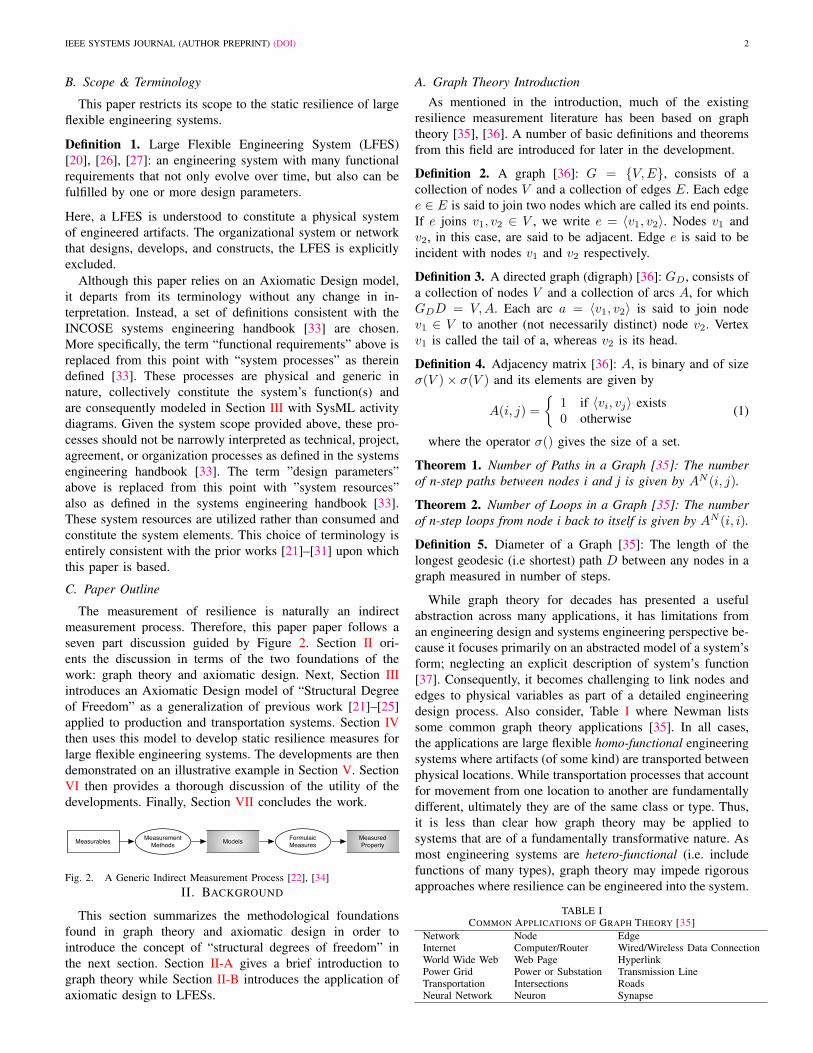
The measurables described in the previous subsection maybe practically measured manually [40] or automatically [34]as has been done in a number of practical case studies [22],[40]. In the latter case, the LFES processes and resources areoften found in IT-based management systems such as thosefound in the control centers of production shop floors, trafficoperators, power grid operators, and water utilities. Figure 3,provides a SysML example of system processes, resources, andtheir allocation via swim lanes. Such an approach implicitlydefines an ontological basis for the system’s transformationand holding processes [22], [41].

C. Sequence-Independent Structural Degrees of Freedom

The concept of structural degrees of freedom was initiallyintroduced on the basis of an analogy with mechanical degreesof freedom [21]–[26]. The heart of the concept rests inthe realization that an allocated action ewv ∈ E (in theSysML activity diagram sense) [42] can be defined for eachfeasible combination of system process pw and resource rv .Naturally, the existence of ewv in the LFES is representedby JS(w, v) = 1. SysML classifies actions on the basis ofwhether they are streaming or nonstreaming. In the case of



Distill Water Distill Water[Activity] act [ ]

«continuous»discharge:Residue

{stream}

«continuous»cold dirty: H2O

{stream}

«continuous»external: Heat

{stream}

«continuous»pure:H2O{stream}

a3: Condense Steam

steam:H2O

recovered:Heat

pure H2O

shutdown

a1: Heat Water

recovered: Heatcold dirty: H2O

hot dirty: H2O

a2: Boil Water

steam dirty: H2O

predischarge: Residueexternal:Heat

hot dirty: H2Oa4: Drain Residue

predischarge:Residue

«allocate»evaporator: Boiler

«allocate»condensor: Heat Exchanger

«allocate»drain: Valve

of4

of8

of2

of3

of5

of6

of7

of1

Fig. 3. Example: System Processes, Resources & Allocation [26]

the former, the allocated action would be described by acontinuous time differential equation [43], [44]. In the case ofthe latter, the allocated action would be described as a discreteevent [45]. With these notions in mind, reconfigurations anddisruptions can add or remove these allocated actions orpotentially reallocate a process to a resource.

The development of structural degrees of freedom continueswith the introduction of a number constraints as is foundin mechanical degrees of freedom. Here, the constraints arediscrete and can apply in the operational time frame so as toeliminate actions from the action set. These constraints are saidto be scleronomic as they are independent of action sequence.Such constraints can arise from any phenomenon that reducesthe capabilities of a LFES e.g. resource breakdowns, inflexiblyimplemented processes and their control.

Definition 10. LFES Scleronomic Constraints Matrix [21]–[26]: A binary matrix KS of size σ(P )×σ(R) whose elementKS(w, v) ∈ {0, 1} is equal to one when a constraint eliminatesevent ewv from the event set.

From these definitions of JS and KS , follows the definitionof LFES sequence-independent structural degrees of freedom.

Definition 11. LFES Sequence-Independent Structural De-grees of Freedom [21]–[26]: The set of independent actionsES that completely defines the available processes in a LFES.Their number is given by:

DOFS = σ(ES) =

σ(P )∑w

σ(R)∑v

[JS KS ] (w, v) (3)

=

σ(P )∑w

σ(R)∑v

AS(w, v) (4)

In matrix form, Equation 3 can be rewritten in terms of theFrobenius inner product [46].

DOFS = 〈JS , K̄S〉F = tr(JTS K̄S) (5)

JS and KS can be reconstructed straightforwardly fromsmaller knowledge bases that individually address transfor-mation, transportation and holding processes. Pµ = JM �M ,Pη = JH � R, Pγ = Jγ � R. In this case, it follows that[21]–[26]:

JS =

[JM | 0

JH̄

](6)

KS =

[KM | 0

KH̄

](7)

where [21]–[26]

JH̄ =[Jϕ ⊗ 1σ(Pη)

]·[1σ(Pϕ) ⊗ JH̄

]KH̄ =

[Kϕ ⊗ 1σ(Pη)

]·[1σ(Pϕ) ⊗KH̄

] (8)

and 1n is a ones vector of length n. Consequently, transfor-mational (DOFM ) and transportational (DOFH ) degree offreedom measures may be calculated as shown in Table III[21]–[26].

TABLE IIITYPES OF LFES SEQUENCE-INDEPENDENT DEGREE OF FREEDOM

MEASURES [21]–[26]

Measure ProcessElement

ResourceElement

KnowledgeBase

ConstraintMatrix

MeasureFunction

DOFM pµj mk JM KM 〈JM , K̄M 〉FDOFH pηu rv JH KH 〈JH , K̄H〉FDOFH̄ Pγ% rv JH̄ KH̄ 〈JHγ , K̄Hγ〉FDOFS pw rv JS KS 〈JSγ , K̄Sγ〉F

Intuitively, the sequence-independent structural degrees offreedom measure the number of ways that all of the systemprocesses may be executed. They provide a flexible expressionof LFES capabilities in the design and operational phases.From an axiomatic design perspective, the usage of knowl-edge bases facilitates further detailed engineering design [20].The constraints matrix captures the potential for resourcebreakdowns and inflexibly implemented processes either phys-ically or informatically in associated control and managementstructures. Additionally, from a graph theory perspective, theknowledge base forms a bipartite graph which may experiencenode or edge addition or elimination during operation. In thenext section, a graph will be formed with structural degreesof freedom representing the nodes.

D. Sequence-Dependent Structural Degrees of Freedom

The previous subsection recalled the development ofsequence-independent structural degrees of freedom. A LFES,however, has constraints that introduce dependencies in thesequence of actions. A new measure is required for thesequence-dependent capabilities of the LFES [21]–[26].

Example 2. Reconsider Figure 3 [26]. Each solid line betweenactivities represents a feasible sequence or pair of activities.Unconnected activities effectively have a design constraint thatprohibits their sequential operation.

Definition 12. LFES Sequence-Dependent Structural Degreesof Freedom [21]–[26]: The set of independent pairs of actionszψ1ψ2 = ew1v1ew2v2 ∈ Z of length 2 that completely describethe system language. The number is given by:

DOFρ = σ(Z) =

σ(ES)∑ψ1

σ(ES)∑ψ2

[Jρ Kρ](ψ1, ψ2) (9)

=

σ(ES)∑ψ1

σ(ES)∑ψ2

[Aρ](ψ1, ψ2) (10)

where Jρ and Kρ are defined below.



TABLE IVTYPES OF SEQUENCE-DEPENDENT PRODUCTION DEGREE OF FREEDOM MEASURES [24]–[26]

Type Measures Processes Resources Knowledge Base ConstraintMatrix

PerpetualConstraint

Measure Function

I DOFMMρ PµPµ M,M JMMρ =[JM · K̄M

]V [JM · K̄M

]V TKMMρ K1 = K2 〈JMMρ, K̄MMρ〉F

II DOFMHρ PµPη M,R JMHρ =[JM · K̄M

]V [JH · K̄H

]V TKMHρ k1 − 1 =

(u1 − 1)/σ(BS)〈JMHρ, K̄MHρ〉F

III DOFHMρ PηPµ R,M JHMρ =[JH · K̄H

]V [JM · K̄M

]V TKHMρ k1 − 1 =

(u1 − 1)&σ(BS)〈JHMρ, K̄HMρ〉F

IV DOFHHρ PηPη R,R JHHρ =[JH · K̄H

]V [JH · K̄H

]V TKHHρ (u1−1)%σ(BS) =

(u2 − 1)/σ(BS)〈JHMρ, K̄HMρ〉F

ALL DOFρ PP R,R Jρ =[JS · K̄S

]V [JS · K̄S

]V TKρ All of the Above 〈JHMρ, K̄HMρ〉F

Definition 13. LFES Rheonomic knowledge base [24]–[26]:A square binary matrix Jρ of size σ(P )σ(R) × σ(P )σ(R)whose element Jρ(ψ1, ψ2) ∈ {0, 1} is equal to one when stringzψ1,ψ2 exists. It may be calculated directly as

Jρ =[JS · K̄S

]V [JS · K̄S

]V T(11)

where ()V is shorthand for vectorization (i.e. vec()).

Definition 14. LFES Rheonomic Constraints Matrix Kρ [24]–[26]: a square binary constraints matrix of size σ(P )σ(R) ×σ(P )σ(R) whose elements K(ψ1, ψ2) ∈ {0, 1} are equal toone when string zψ1ψ2 = ew1v1ew2v2 ∈ Z. is eliminated andwhere ψ = σ(P )(v − 1) + w.

Unlike its scleronomic counterpart where a zero matrixis possible, the rheonomic production constraints matrix hasthe perpetually binding constraints described in Table IV.These ensure that the origin and destination of consecutiveevents match. Accurately keeping track of these constraintssimultaneously is challenging. The final calculation of theseminimal constraints is most easily implemented in a scalarfashion using FOR loops while adhering to the followingrelationships of indices. ψ = σ(P )(v − 1) + w. v = k∀k = [1 . . . σ(M)]. w = [σ(Pη)(g − 1) + u] + j [24], [26].

As with sequence-independent structural degrees of free-dom, sequence-dependent structural degrees of freedom maybe classified in terms of their transformational and transporta-tional variants. The calculation of the four types of measures issummarized in Table IV and maintains an intuitive symmetry[24]. In practice, the formation of the associated constraintsmatrices KMMρ, KMHρ, KHMρ,KHHρ is an extra compu-tational expense if Kρ has already been formed. Instead, theassociated rheonomic production degree of freedom measurescan be calculated by the appropriate replacement of JM or JH̄with a zero matrix in Equation 6 [24].

Intuitively, the sequence-dependent structural degrees offreedom measure the number of ways that pairs of system pro-cesses may be executed. In other words, the system languageL can be described equally well in terms of the Kleene closure[45] of the sequence-independent and sequence-dependentstructural degrees of freedom.

L = E∗S = Z∗ (12)

From a graph theory perspective, Equation 11 shows thatthe sequence independent structural degrees of freedom areexplicitly vectorized (as is commonly done with mechanicaldegrees of freedom). Furthermore, boolean difference of the

rheonomic knowledge base and constraints matrix forms anadjacency matrix Aρ between nodes defined as structuraldegrees of freedom.

E. Service-Specific Structural Degrees of Freedom

While it is important to quantify the capabilities of a LFES,it is even more important to assess how well these capabilitiesare matched to the services that it intends to offer. This isespecially important in the context of resilience measurementwhere either the required services or the existing capabilitiesmay be changed. Furthermore, resilience is often measuredwith respect to a certain performance property [47]; thusimplicitly defining one or more services of interest. Thissubsection builds upon the efforts of the previous sections todevelop service-specific structural degrees of freedom. Intu-itively speaking, the required services select out the sequence-independent structural degrees of freedom and the mathemati-cal form of the associated measure is developed on that basis.To begin, the set of services is simplistically modeled so thatthe service-specific structural degree of freedom measures maybe developed later.

1) Service Modeling: Before a treatment of service-specificstructural degrees of freedom can be initiated, a systematicapproach to describing services is required. For the sakeof simplicity, the scope of this work restricts itself to aclass of services that do not require the mixing/assemblyof heterogeneous artifacts, or the disjoining/separation of thesame. The interested reader is referred to [22] for work thataddress such types of services.

A LFES may provide a set of services L = {l1, . . . , lσ(L)}where each service li has its associated set of service activitiesexli ∈ Eli which when all are completed result in the deliveryof the service.

Definition 15. Service Activity [22], [24], [26]: A specifictransformation process that may be applied as a part of largerservice.

Consequently, the delivery of the service is described as asequence of service activities [22], [24], [26]:

zli = ex1liex2li . . . exσ(Eli )li(13)

Example 3. Table V provides concrete examples of servicesfor production, transportation, power grid and water distribu-tion systems.

These examples offer a number of fundamental insights.First, it is important to note that this work implicitly assumes



TABLE VEXAMPLE SYSTEM SERVICES IN LFESS [26]

Transportation: {Enter passenger at the origin station, Exit the passengerat the destination}

Power Grid: {Generate electricity at the origin, Consume the elec-tricity at the destination}

Water Dis-tribution:

{Extract the water at the origin, Treat the water, De-grade the water through use, Dispose of the water atthe destination}

Production: {Enter the part to an input buffer, Mill the part, Drill ahole in the part, Polish the part, Exit the part from anoutput buffer}

that the LFES is an open system. As such all of the servicesdescribed above begin with an entrance of some artifact andend with its exit. Furthermore, water distribution and produc-tion systems require more careful thought given the potentialheterogeneity of transformation processes and their artifacts.Finally, all of the systems do not fundamentally requiretransportation processes because all transformation processesrequired by the service could conceivably be realized in onelocation. This generalization is true even for transportationsystems for the trivial case that the passenger’s desired originand destination are the same.

2) Service Activity Feasibility: The feasibility of a givenservice on an activity-by-activity basis follows straightfor-wardly from the introduction of two feasibility matrices.

Definition 16. Service Transformation Feasibility Matrix Λµi[22], [24], [26]: For a given service li, a binary matrix of sizeσ(Eli) × σ(Pµ) whose value Λµi(x, j) = 1 if exli realizestransformation process pµj .

Definition 17. Service Transportation Feasibility Matrix Λγi[22], [24], [26]: A binary row vector of size 1×σ(Pγ) whosevalue Λγi(g) = 1 if product li can be held by holding processpγg .

Note that because the service model only includes activitiesof a transformative nature, Λγi only marks feasibility betweenthe service as a whole and the set of holding processes [22],[24].

3) Calculation of Service-Specific Structural Degrees ofFreedom: From these definitions, it is straightforward to mea-sure the number of LFES service-specific structural degreesof freedom. Λµi and Λγi must first be used to produce anumber of “selector” matrices that are equal in size to theircorresponding LFES (scleronomic) knowledge base. Whichone is used depends on the scope of interest; be it the type ofprocess (e.g. transformation or transportation) or the desiredscale (i.e. a single service activity, a whole service, or thewhole set of services). Table VI summarizes the definition andformulation of the multiple types of service selector matrices[24], [26].

From these definitions, it is straightforward to measure thenumber of LFES service-specific structural degrees of freedom[24], [26].

DOFLS = 〈ΛSL · JS , K̄S〉F (14)

As mentioned at the beginning of the section, this intuitiveform of service-specific degrees of freedom shows that theservices effectively select out the structural degrees of freedomprovided by the LFES [24], [26].

TABLE VITYPES OF SERVICE SELECTOR MATRICES [22], [24], [26]

Symbol Formula Scope

ΛMxi[eTxΛµi

]T1σ(M)T Service Activity – Transfor-

mation

ΛMi

σ(EL)∨x

Λµi

T1σ(M)T Service – Transformation

ΛML

σ(L)∨i

σ(EL)∨x

Λµi

T1σ(M)T Service Line – Transforma-tion

ΛHi[Λγi ⊗ 1σ(Pη)T

]T1σ(R)T Service – Transportation

ΛHi

σ(L)∨i

Λγi

⊗ 1σ(Pη)T

T1σ(R)T Service – Transportation

ΛSxi

[ΛMxi | 0

ΛHi

]Service Activity – Transfor-mation & Transportation

ΛSMxi

[ΛMxi | 0

0

]Service Activity – Transfor-mation

ΛSi

[ΛMi | 0

ΛHi

]Service – Transformation &Transportation

ΛSHi

[0 | 0

ΛHi

]Service – Transportation

ΛSL

[ΛML | 0

ΛHL

]Service Line – Transforma-tion & Transportation

F. Relevance of Structural Degrees of Freedom to ResilienceMeasurement

The structural degree of freedom measures have a directrelevance to resilience measurement. This is because theyprovide a quantitative description of the system “reconfigura-tion” potential [21], [34], [34]; be it an arbitrary disruption orrestoration of the system’s capabilities. Such a reconfigurationprocesses would be mathematically described by [21], [24],[26], [48]:

(JSo ,KSo ,Kρo)→ (JS ,KS ,Kρ) (15)

The static resilience or survivability measures devel-oped in the next section depend on the performancedegradation arising from the reconfiguration process de-scribed by Equation 15 and implicitly assume thatDOFρo(JSo ,KSo ,Kρo) ≥ DOFρ(JS ,KS ,Kρ). In that sense,it assumes that (JS ,KS ,Kρ) are associated with closed setsof processes and resources. That said, future work on dynamicresilience or “recovery” can loosen this assumption and allowfor an expansion in these sets to achieve greater resilience.

IV. DEVELOPMENT OF STATIC RESILIENCE MEASURES

The background provided by the previous two sections al-low for the development of static resilience measures for largeflexible engineering systems. Many resilience measures in theexisting literature are based upon some form of calculation ofthe shortest path length through a traditional graph [49]–[52].Similarly, the static resilience measures proposed in this workdepend on paths through a graph as well. In contrast, however,the measures derive from the number rather than the lengthof those paths. Furthermore, the paths are through a graphbased upon nodes defined as structural degrees of freedomrather than simply locations as is often done in traditionalgraph theory. This section proceeds in two parts. SectionIV-A enumerates the number of paths for a service offeredby an LFES. Section IV-B then proposes the static resiliencemeasures.



A. Path Enumeration in Large Flexible Engineering Systems

The development of static resilience measures depends onthe enumeration of the number of feasible paths for eachof the services provided by the LFES. The first step in thiscalculation is the translation of the service string in Equation13 to an equivalent string composed of structural degrees offreedom. Because the service feasibility of transformation andtransportation processes is fundamentally different, the newequivalent string must also alternate between the two types ofdegrees of freedom [22], [24], [27].

z = eµj1mk1 [eγϕ1rv1

]∗Deµj2mk2 [eγϕ2rv2

]∗D . . . eµjσ(Eli )mkσ(Eli )

(16)where the exponent of an activity is used to denote the numberof times it is repeated, and ∗D denotes the repetition betweenzero and D times where D is the diameter of the transportationnetwork of the LFES as defined in Definition 5. For simplicity,Equation 16 can be rewritten explicitly in terms of its repeatingpattern: [

eµjxmkx [eγϕ1rv1

]∗Deµj2mk2

]σ(Eli )

(17)

Example 4. The string in Equation 17 is overly general formost LFESs [27]. It is useful to specialize it for each of thefour example LFESs discussed in this work:

Transportation [27]: The passenger must enter at the originstation, take a number of transportation degrees of freedomand then leave at the destination. Therefore, Equation 16 cancollapse to:

eµj1mk1 [eγϕ1rv1]∗Deµj2mk2 (18)

Power Grid [27]: The electricity must be generated at apower plant, pass through a number of power lines and then beconsumed at a destination. Therefore, power grids also followthe string in Equation 18.

Production [27]: Production system’s naturally minimizetransportation degrees of freedom because they are viewedas non-value adding. Good production system design practiceallows at most one transportation process between any twotransformation degrees of freedom. Therefore, Equation 17 cancollapse to [27]:[

eµjxmkx [eγϕ1rv1]eµj2mk2

]σ(Eli )

(19)

Note that this string still encompasses the potential for suc-cessive transformation events because the transportation eventsinclude “null processes” where no motion occurs at a systemresource.

Water Distribution [27]: Taken alone, the potable waterdistribution network resembles the transportation and powergrid systems as in Equation 18. However, when the waterdistribution system is taken to include storm drains, wastewa-ter, and recycled water, then the full string in Equation 17 isrequired.

The next step in path enumeration is to rewrite Equation 17in terms of sequence-dependent structural degrees of freedom

using Equation 12 [27].[zψMxψH [zHH ]∗D−1zψMx+1

ψH

]σ(Eli )−1

(20)

where zψMxψH , zHH , and zψMx+1ψH are Type II, III and IV

sequence-dependent structural degrees of freedom respectively(See Table IV). This relatively compact form explicitly statesin terms of the sequence-dependent structural degrees offreedom the paths through a LFES that would make a givenservice feasible.

The enumeration of these paths is straightforward usingTheorem 1. To that effect, an adjacency matrix is written foreach of the three types of sequence dependent structural de-grees of freedom in Equation 20. This requires the applicationof Equation 9 as specialized by Tables III, IV, and VI. Forany given service i [27],

AMHx1ρ =[ΛSMx1 · JSM · K̄SM

]V [ΛSH · JSH · K̄SH

]V T Kρ

(21)

AHHρ =[ΛSH · JSH · K̄SH

]V [ΛSH · JSH · K̄SH

]V T Kρ

(22)

AHMx2ρ =[ΛSH · JSH · K̄SH

]V [ΛSMx2 · JSM · K̄SM

]V T Kρ

(23)

where x1 and x2 are the indices of sequential serviceactivities. x2 = x1 + 1. These adjacency matrices are thenmultiplied together following Equation 20 to give the numberof paths through a LFES for a given service i

DOFPi =

σ(ES)∑ψ1

σ(ES)∑ψ2

[APi

](ψ1, ψ2) (24)

where

APi =

D∑d=1

[(AMHxρ)

(Ad−1HHρ

)(AHMx+1ρ)

]σ(Eli )−1

(25)

Note that the summation over d is required here because theirmay exist transportation paths of length one up to D − 1between successive transformations [25].

Example 5. As expected, this formula is overly general formost LFESs [27]. It is useful to specialize it for each of thefour example LFESs discussed in this work:

Transportation/Power/Potable Water Distribution [27]:

APi =

D∑d=1

[(AMHxρ)

(Ad−1HHρ

)(AHMx+1ρ)

](26)

which confirms the result in [25].Production [27]:

APi =

[(AMHxρ) (AHMx+1ρ)

]σ(Eli )−1

(27)

which confirms the result in [24].

Remark. For the application of resilience measurement, it isoften important to distinguish between the number of trans-portation paths and the number of simple transportation paths(i.e. without loops). Intuitively speaking, transportation loopsrepresent a type of unuseful redundancy. For this purpose, it



may be necessary to eliminate the number of loops from thecalculation of Equation 25. This can be done straightforwardlyby eliminating the diagonal at each power of AHHρ. InsteadAD−1HHρ can be replaced with AD−1

HHSρ which is defined recur-sively [27]:

AnHHSρ =[An−1HHSρ − diag(An−1

HHSρ)]

[AHHSρ] (28)

AHHSρ =AHHρ − diag(AHHρ)

B. Static Resilience Measures

Returning to Figure 1, this work is concerned with staticresilience measures which effectively quantifies survivabilityor the level of immediate degradation caused by a disruptionrepresented as a change in (JS , KS ,Kρ). Furthermore, theperformance of the service depends on the existence of acomplete path for its realization. Therefore, a static resiliencemeasure can be defined as a function of the existence or num-ber of paths that realize a service which are in turn a functionof the structural degrees of freedom. The section proceedsby defining the concept of performance then proposing tworesilience measures.

1) Definition of Performance: In the context of this work,the engineering performance of an LFES depends purely onits static structure. Consider a service i, that begins with DOFeψ1 and ends with eψ2 . It delivers a quantity Qi(ψ1, ψ2) worthof a valuable artifact. The performance of that service is givenby [27]:

EPi =

σ(ES)∑ψ1

σ(ES)∑ψ2

Qi(ψ1, ψ2) · bi [APi(ψ1, ψ2)] (29)

where bi() is the binary function that returns 1 for all positivequantities and zero otherwise. Here, it is assumed that thenumber of paths for the service is not as important as thesimple existence of such a path. As such, it assumes that eachpath is not capacity limited in Q. For the full engineeringperformance of the LFES over all services, it is necessary tolinearly combine this measure with those of the other services[27].

EP =

σ(L)∑i

σ(ES)∑ψ1

σ(ES)∑ψ2

ciQi(ψ1, ψ2) · bi [APi(ψ1, ψ2)] (30)

where ci is a measure of value of the ith service such as utility,cost or profit that harmonizes the units of all Qi.

In the context of this work, it is also useful to write theengineering performance measure explicitly in terms of theknowledge base and constraint matrices (JS ,KS ,Kρ). Withthe change of notation APi(ψ1, ψ2) = APiψ1ψ2 [27],

EP =

σ(L)∑i

σ(ES)∑ψ1

σ(ES)∑ψ2

ciQi(ψ1, ψ2)·bi [APiψ1ψ2(JS ,KS ,Kρ)]

(31)Because the LFES’s dynamics in terms of constitutive, conti-nuity and compliance relations have not been modeled, Qi ismodeled as a constant rather than as a function of the structuraldegrees of freedom. Nevertheless, the ability to provide Qidoes require the existence of at least one service path and sostudying the presence of such a path is a logical first step.

2) Actual Resilience: The actual engineering resilience(AER) with respect to a particular disruption that takesthe system through the transformation: (JSo ,KSo ,Kρo) →(JS ,KS ,Kρ) can now be defined straightforwardly [27].

AER =EP (JS ,KS ,Kρ)

EP (JSo ,KSo ,Kρo)(32)

This actual resilience measure benefits from the binary func-tion bi(). As expected, LFESs that exhibit some path redun-dancy for their services will not suffer from performancedegradation. That said, the bi() also hides the effect ofredundancy elimination caused by successive disruptions andso is not the most accurate predictor of the LFES’ “health”towards future disruptions.

3) Latent Engineering Resilience: To address the limita-tions of the actual resilience measure, a latent engineeringresilience measure is proposed [27]. LER=

σ(L)∑i

σ(ES)∑ψ1

σ(ES)∑ψ2

ciQi(ψ1, ψ2) · [APiψ1ψ2(JS ,KS ,Kρ)]

[APiψ1ψ2(JSo ,KSo ,Kρo)]

EP (JSo ,KSo ,Kρo)(33)

Here, the LER measure degrades gracefully with the transfor-mation (JSo ,KSo ,Kρo)→ (JS ,KS ,Kρ) because of the ratioof actual enumerated paths to the prior enumerated paths. Itmay be used to show how a given disruption eliminates somebut not all of the paths of a given service.

V. ILLUSTRATIVE EXAMPLE

Based on the discussion of the previous section, a largeflexible engineering system with several types of functions ischosen for an illustrative example. This choice demonstratesthe analytical capability of the proposed measures relative tothose applicable to homo-functional systems. As mentioned inExamples 3 and 4, production systems provide an extra level offunctional heterogeneity that is less apparent in transportation,electric power and potable water distribution. To this end, the“Starling Manufacturing System” is taken as the test case forits functional heterogeneity and redundancy and its resourceflexibility while maintaining a moderate size [21], [22], [24],[26], [27].

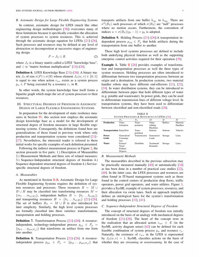
The system produces customized bird feeders from cylin-drical wooden components. In this example, customers canchoose between bird feeders of red and yellow color, and smalland large radii. The wooden cylinders are turned for slots andtabs, milled, laminated, and painted. All product variants havean injection molded dome roof and a base which doubles as abird perch. These components are manually snapped onto thecylindrical bird feeders after production and are not furtherdiscussed in this example.

The production system itself is considered in three con-figurations that includes machining, lamination, and paintingmachines. Figure 4(a) shows the initial configuration, Figure4(b) adds a second machining station, and Figure 4(c) makesall three value-adding resources redundant. Two shuttles trans-port the cylinders between the machines and buffer. The firsthas a flexible fixture which accommodates both radius sizeswhile the second can only carry cylinders of small radius.



MillingStation 1

LaminationStation 1

PaintingStation 1

OutputBuffer

InputBuffer

(a) Phase I

MillingStation 2

MillingStation 1

LaminationStation 1

PaintingStation 1

OutputBuffer

InputBuffer

(b) Phase II

MillingStation 2

LaminationStation 2

MillingStation 1

PaintingStation 2

LaminationStation 1

PaintingStation 1

OutputBuffer

InputBuffer

(c) Phase IIIFig. 4. Starling manufacturing system in three configurations

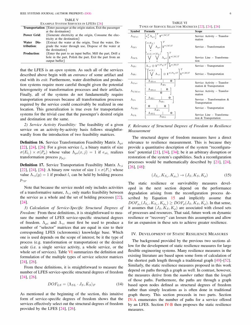
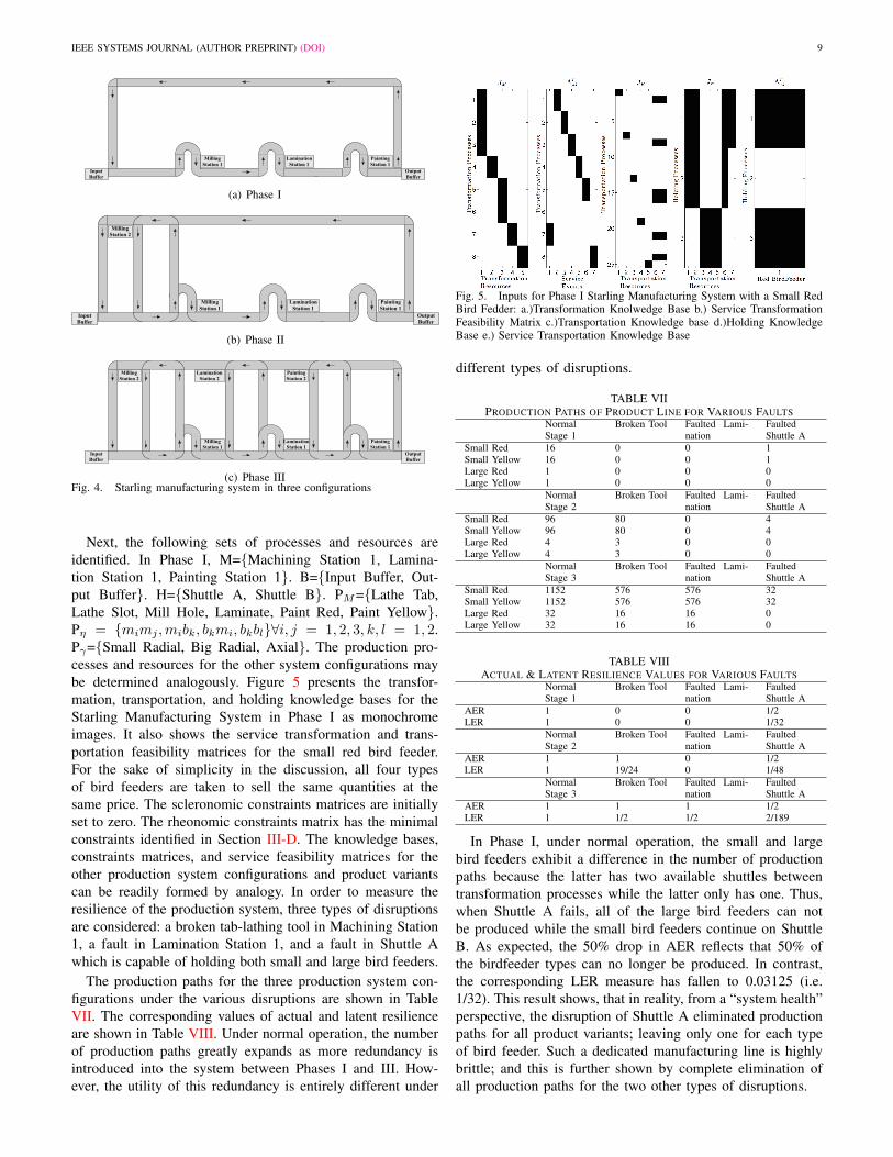
Next, the following sets of processes and resources areidentified. In Phase I, M={Machining Station 1, Lamina-tion Station 1, Painting Station 1}. B={Input Buffer, Out-put Buffer}. H={Shuttle A, Shuttle B}. PM={Lathe Tab,Lathe Slot, Mill Hole, Laminate, Paint Red, Paint Yellow}.Pη = {mimj ,mibk, bkmi, bkbl}∀i, j = 1, 2, 3, k, l = 1, 2.Pγ={Small Radial, Big Radial, Axial}. The production pro-cesses and resources for the other system configurations maybe determined analogously. Figure 5 presents the transfor-mation, transportation, and holding knowledge bases for theStarling Manufacturing System in Phase I as monochromeimages. It also shows the service transformation and trans-portation feasibility matrices for the small red bird feeder.For the sake of simplicity in the discussion, all four typesof bird feeders are taken to sell the same quantities at thesame price. The scleronomic constraints matrices are initiallyset to zero. The rheonomic constraints matrix has the minimalconstraints identified in Section III-D. The knowledge bases,constraints matrices, and service feasibility matrices for theother production system configurations and product variantscan be readily formed by analogy. In order to measure theresilience of the production system, three types of disruptionsare considered: a broken tab-lathing tool in Machining Station1, a fault in Lamination Station 1, and a fault in Shuttle Awhich is capable of holding both small and large bird feeders.

The production paths for the three production system con-figurations under the various disruptions are shown in TableVII. The corresponding values of actual and latent resilienceare shown in Table VIII. Under normal operation, the numberof production paths greatly expands as more redundancy isintroduced into the system between Phases I and III. How-ever, the utility of this redundancy is entirely different under

Fig. 5. Inputs for Phase I Starling Manufacturing System with a Small RedBird Fedder: a.)Transformation Knolwedge Base b.) Service TransformationFeasibility Matrix c.)Transportation Knowledge base d.)Holding KnowledgeBase e.) Service Transportation Knowledge Base

different types of disruptions.

TABLE VIIPRODUCTION PATHS OF PRODUCT LINE FOR VARIOUS FAULTS

NormalStage 1

Broken Tool Faulted Lami-nation

FaultedShuttle A

Small Red 16 0 0 1Small Yellow 16 0 0 1Large Red 1 0 0 0Large Yellow 1 0 0 0

NormalStage 2


FaultedShuttle A


NormalStage 3


FaultedShuttle A


TABLE VIIIACTUAL & LATENT RESILIENCE VALUES FOR VARIOUS FAULTS

NormalStage 1


FaultedShuttle A

AER 1 0 0 1/2LER 1 0 0 1/32

NormalStage 2


FaultedShuttle A

AER 1 1 0 1/2LER 1 19/24 0 1/48

NormalStage 3


FaultedShuttle A

AER 1 1 1 1/2LER 1 1/2 1/2 2/189

In Phase I, under normal operation, the small and largebird feeders exhibit a difference in the number of productionpaths because the latter has two available shuttles betweentransformation processes while the latter only has one. Thus,when Shuttle A fails, all of the large bird feeders can notbe produced while the small bird feeders continue on ShuttleB. As expected, the 50% drop in AER reflects that 50% ofthe birdfeeder types can no longer be produced. In contrast,the corresponding LER measure has fallen to 0.03125 (i.e.1/32). This result shows, that in reality, from a “system health”perspective, the disruption of Shuttle A eliminated productionpaths for all product variants; leaving only one for each typeof bird feeder. Such a dedicated manufacturing line is highlybrittle; and this is further shown by complete elimination ofall production paths for the two other types of disruptions.



In Phase II, an additional milling station provides redun-dancy for three transformation processes: lathe tab, latheslot, and mill hole. Setting aside the transportation systemredundancy, the number of paths in normal operation shouldgrow by 23 = 8. However, it only grows by a factor of 4 forthe large bird feeders because they can be transferred fromthe second milling station to the first but not vice versa. Thedisruption of Shuttle A has a similar effect in Phase II asin Phase I. The AER drops by 50% and the LER falls to aneven smaller value to reflect that an even greater percentage ofthe production paths have been eliminated as a result of thedisruption. That said, the addition of the redundant millingstation has dramatically improved the AER and LER valuesin response to a broken tool. The zero AER and LER valuesin response to a fault in the lamination station highlight theproduction system’s vulnerability. Collectively, these resultsshow that adding redundancy must be done judiciously. Inthis case, tools may break often and so redundancy there maybe extremely valuable. It’s also worth noting that an additionalmilling station adds three new structural degrees of freedomwhereas an additional lamination station would only add one.The proposed AER and LER measures thus have the potentialto objectively inform investment decisions in how to upgradethe LFES.

In Phase III, all of the system’s resources are redundant– but not for all products. The large bird feeders are stillentirely disrupted by the failure of Shuttle A and this issimilarly reflected in the AER and LER values. Because, thestructural degree of freedom approach differentiates systemresources in terms of their processes and their applicability toservices, system vulnerabilities can be more easily resolved.Interestingly, the need for resilience in production systems maygo counterflow to lean manufacturing trends where non-valueadding processes were systematically eliminated. In this case,the lack of redundancy in the transportation system eliminatesthe utility of the other forms of redundancy for half of theproduct line. For the other two disruptions, the results arepredictable and intuitive. The AER measure provides a valueof 1 to show that all the products can continue to be producedfeasibly, while the LER measure gives a value of 0.5 to reflectthe corresponding loss in the percentage of production paths.

VI. DISCUSSION

This section discusses some of the advantages of the pro-posed resilience measures relative to the existing literature.

The measurement of resilience as an output in response toa disruption as an input is a natural first step. However, whencomplex simulation packages are used for this purpose [5],[14], [16], [18], [19], [53], they effectively become “black-boxes” that do not necessary shed light as to why a particulardisruption leads to a particular change in performance. Thepredictive capability of such black-box measurement is partic-ularly uncertain for large complex systems and often requiresexhaustive simulation. In contrast, the proposed resiliencemeasures provide a measurement method based upon ab-stracted physical models which provide an advisory capabilityon how to best improve the system resilience. That is not tosay that these measures inform why disruptions occur. Rather,

they inform why a particular disruption affects the systemperformance more than another.

The proposed resilience measures also present a useful levelof abstraction in successive iterations of design and planning.Focusing on the specifics of a system’s dynamic equationsof motion in a first pass analysis, especially when the fullconstitutive relations may not yet be fully known, masksthe strengths and weaknesses of the underlying structure.If necessary at a later stage, the engineering performancemeasure in Equation 30 can be detailed such that Qi(ψ1, ψ2)depends explicitly on the structural degrees of freedom. Suchan approach is consonant with conventional industrial practiceof N-1 contingency analysis [54] in power grids whose resultsoften depend more on the sparsity of the bus admittance matrixthan the values of the impedances and bus injections. Similarly,this approach can be extended into a discrete-event systemsimulation but provides analytical capability at a higher levelof abstraction prior to the implementation of a full simulation.

InputBuffer

OutputBuffer

MachiningStation

Lamination Station

PaintingStation

Fig. 6. Traditional (red) & Structural Degree of Freedom-based (blue) Graphsfor Starling Manufacturing System in Phase I.

While the proposed measures incorporate many of theconcepts found in the existing graph theoretic resilience mea-surement literature, the most fundamental difference is that thegraphs presented in this work have nodes defined as structuraldegrees of freedom rather than simply locations. Figure 6highlights the differences between the two approaches with atraditional graph colored in red while the structural degree offreedom based graph colored in blue. Naturally, the values ofgraph theoretic measures like centrality would differ betweenthe two graphs. The new approach allows for the explicitdescription of multiple modes of transport (i.e. demonstratedby the nearly parallel lines between buffers) and resources withmultiple transformation process (i.e. demonstrated by clustersaround each buffer). In that regard, Axiomatic Design [20]and SysML [42] have the potential to bridge the gap fromabstract graph theoretic descriptions to more well-establishedengineering practice. Indeed, the application of model-basedsystems engineering can allow for the axiomatic design knowl-edge bases to be developed or mined automatically even forvery large scale systems. In such an instance, sparse matrixmethods can be applied to take advantage of the sparsity ofthe knowledge bases and constraint matrices [25], [55]. It isimportant to note that the graph theory community already haswell established case studies for graphs on the order of 107

nodes [56]. That said, the application of the axiomatic design



model at multiple levels of functional and physical abstractionis useful to tackle problems of particularly large scale.

That said, the proposed resilience measures share manyconcepts found in the existing graph theoretic resilience mea-surement literature. First, as demonstrated by the illustrativeexample, the measures proposed here on the basis of service-specific paths are consonant with resilience measures basedupon degree and eigenvector centrality [49], [52]. Service-specific paths are chosen over centrality because they may bemore easily linked to physical values that provide differentlevels of value. Second, the use of paths in the proposedmeasures also agree with resilience measures based upon con-nectedness [11], [17], [57]–[61]. While such measures are im-portant in transportation and communication networks whereevery location must be linked, many resilience improvementstrategies neither require nor encourage graph connectedness.In power grids, for example, the recent literature encouragesthe design and operation of multiple microgrids which canconnect and disconnect from each other while each servingtheir local demand for power [62], [63]. More fundamentally,electrical load can be served with onsite generation andwithout a power grid at all. Similarly, many regions do notrequire water grids because of the existence of local wellsand lakes. Also similarly, production systems have long beendesigned and operated as manufacturing cells with either staticor dynamic configurations. The proposed work is also similarto resilience measures based upon shortest path length [49]–[52]. The dependence on the number rather than the length ofthe paths takes into consideration LFESs where the valuableartifact travels exceptional fast. For example, angular stabilityoscillations caused by an outage in Florida could be felt inMinnesota in less than three seconds [64]. Similarly, fiber opticnetworks rely on information transmission at the speed of light.

VII. CONCLUSION

This paper has proposed actual and latent engineering re-silience measures for large flexible engineering systems. Thisdevelopment was founded upon graph theory, and axiomaticdesign for large flexible engineering systems. Central to thedevelopment was the concept of structural degrees of free-dom as the available combinations of systems processes andresources which could be measured individually to describesystem capabilities or measured sequentially to give a senseof the skeleton of a system’s behavior. It was these sequence-dependent degrees of freedom that were used to enumerateservice paths through a LFES. Each service path may beviewed as a value chain through an LFES along which quan-tities of valuable artifacts flow. Therefore, this work comparedthe value and quantity of service paths before and after adisruption as measures of static resilience – or survivability.

The work presented in this paper leaves open many op-portunities for future work. First, this work can be directlyapplied to hetero-functional LFES’s such as tthe energy-waternexus [32], [65], [66], and the transportation electrification[25], [28]. Second, some faults may not be binary and maylead to impaired rather than fully disabled functionality. Third,this work can be extended to address the dynamic aspects

of resilience. To that effect, the recent work on reconfigura-tion processes [48] may be applied as a promising avenuefor future developments. Furthermore, the Axiomatic Designknowledge base and the associated structure degree of freedomof measures have been recently used in the design of multi-agent systems in power systems [29], [30], [62], [63] andthe manufacturing systems domain [31]. Finally, the authorsbelieve that this work has direct application to resilient controlsystems and resilient human operation in LFESs that possessa significant amount of control, automation, and intelligence.

REFERENCES

[1] D. A. Reed, K. C. Kapur, and R. D. Christie, “Methodology for assessingthe resilience of networked infrastructure,” IEEE Systems Journal, vol. 3,no. 2, pp. 174–180, Jun. 2009.

[2] E. Hollnagel, D. D. Woods, and N. Leveson, Resilience Engineering:Concepts and Precepts, kindle edi ed. Aldershot, U.K.: AshgatePublishing Limited, 2006.

[3] S. M. Rinaldi, J. P. Peerenboom, and T. K. Kelly, “Identifying, un-derstanding, and analyzing critical infrastructure interdependencies,”Control Systems, IEEE, vol. 21, no. 6, pp. 11–25, 2001.

[4] A. M. Madni and S. Jackson, “Towards a conceptual framework forresilience engineering,” IEEE Systems Journal, vol. 3, no. 2, pp. 181–191, 2009.

[5] B. M. Ayyub, “Systems resilience for multihazard environments: Defi-nition, metrics, and valuation for decision making,” Risk Analysis, pp.1–16, 2013.

[6] Y. Y. Haimes, K. Crowther, and B. M. Horowitz, “Homeland securitypreparedness: Balancing protection with resilience in emergent systems,”Systems Engineering, vol. 11, no. 4, pp. 287–308, 2008.

[7] {The White House: Office of the Press Secretary}, “Presidential PolicyDirective: Critical Infrastructure Security and Resilience (PPD-21),” TheWhite House, Washington, D.C. United states, Tech. Rep., 2013.

[8] C. S. Holling, “Resilience and Stability of Ecological Systems,” AnnualReview of Ecology and Systematics, vol. 4, no. 1, pp. 1–23, Nov. 1973.

[9] A. Rose, “Economic resilience to natural and man-made disasters:Multidisciplinary origins and contextual dimensions,” EnvironmentalHazards, vol. 7, no. 4, pp. 383–398, 2007.

[10] T. J. Vogus and K. M. Sutcliffe, “Organizational resilience: towardsa theory and research agenda,” in Systems, Man and Cybernetics,2007. ISIC. IEEE International Conference on, ser. IEEE InternationalConference on Systems, Man and Cybernetics, 2007. Vanderbilt OwenGraduate Sch. of Manage., Nashville, USA BT - IEEE InternationalConference on Systems, Man and Cybernetics, 2007, 7-10 Oct. 2007:IEEE, 2008, pp. 3418–3422.

[11] W. Najjar and J.-L. J.-L. Gaudiot, “Network resilience: a measure ofnetwork fault tolerance,” IEEE Transactions on Computers, vol. 39,no. 2, pp. 174–181, Feb. 1990.

[12] J. Diamond, Collapse: How Societies Choose to Fail or Succeed,revised ed. New York NY: Penguin Books, 2011.

[13] A. D. VanBreda, “Resilience Theory : A Literature Review by,” MilitaryPsychological Institute, Pretoria, South Africa, Tech. Rep. October,2001.

[14] R. Francis and B. Bekera, “A metric and frameworks for resilience anal-ysis of engineered and infrastructure systems,” Reliability Engineeringand System Safety, vol. 121, pp. 90–103, 2014.

[15] R. Bhamra, S. Dani, and K. Burnard, “Resilience: the concept, a litera-ture review and future directions,” International Journal of ProductionResearch, vol. 49, no. 18, pp. 5375–5393, 2011.

[16] D. Henry, J. E. Ramirez-Marquez, and J. Emmanuel Ramirez-Marquez,“Generic metrics and quantitative approaches for system resilience as afunction of time,” Reliability Engineering and System Safety, vol. 99,pp. 114–122, Mar. 2012.

[17] J. C. Whitson and J. E. Ramirez-Marquez, “Resiliency as a componentimportance measure in network reliability,” Reliability Engineering& System Safety, vol. 94, no. 10, pp. 1685–1693, Oct. 2009.

[18] K. Barker, J. E. Ramirez-Marquez, and C. M. Rocco, “Resilience-basednetwork component importance measures,” Reliability Engineering andSystem Safety, vol. 117, pp. 89–97, 2013.

[19] R. Pant, K. Barker, and C. W. Zobel, “Static and dynamic metricsof economic resilience for interdependent infrastructure and industrysectors,” Reliability Engineering & System Safety, vol. 125, no. 92-102,2013.



[20] N. P. Suh, Axiomatic Design: Advances and Applications. OxfordUniversity Press, 2001.

[21] A. M. Farid and D. C. McFarlane, “Production degrees of freedom asmanufacturing system reconfiguration potential measures,” Proceedingsof the Institution of Mechanical Engineers, Part B (Journal of Engineer-ing Manufacture), vol. 222, no. B10, pp. 1301–1314, Oct. 2008.

[22] A. M. Farid, “Reconfigurability Measurement in Automated Manufactur-ing Systems,” Ph.D. Dissertation, University of Cambridge EngineeringDepartment Institute for Manufacturing, 2007.

[23] ——, “Product Degrees of Freedom as Manufacturing System Recon-figuration Potential Measures,” International Transactions on SystemsScience and Applications, vol. 4, no. 3, pp. 227–242, 2008.

[24] ——, “An Axiomatic Design Approach to Non-Assembled Produc-tion Path Enumeration in Reconfigurable Manufacturing Systems,” in2013 IEEE International Conference on Systems Man and Cybernetics,Manchester, UK, 2013, pp. 3862 – 3869.

[25] A. Viswanath, E. E. S. Baca, and A. M. Farid, “An Axiomatic DesignApproach to Passenger Itinerary Enumeration in Reconfigurable Trans-portation Systems,” IEEE Transactions on Intelligent TransportationSystems, vol. 15, no. 3, pp. 915–924, 2014.

[26] A. M. Farid, “Static Resilience of Large Flexible Engineering Systems: Part I – Axiomatic Design Model,” in 4th International EngineeringSystems Symposium, Hoboken, N.J., 2014, pp. 1–8.

[27] ——, “Static Resilience of Large Flexible Engineering Systems : PartII – Axiomatic Design Measures,” in 4th International EngineeringSystems Symposium, Hoboken, N.J., 2014, pp. 1–8.

[28] A. Viswanath and A. M. Farid, “A Hybrid Dynamic System Model forthe Assessment of Transportation Electrification,” in American ControlConference 2014, Portland, Oregon, 2014, pp. 1–7.

[29] A. M. Farid, “Multi-agent system design principles for resilient operationof future power systems,” in IEEE International Workshop on IntelligentEnergy Systems, San Diego, CA, 2014, pp. 1–7.

[30] ——, “Multi-Agent System Design Principles for Resilient Coordination& Control of Future Power Systems,” Intelligent Industrial Systems (inpress), vol. 1, no. 1, pp. 1–9, 2015.

[31] A. M. Farid and L. Ribeiro, “An Axiomatic Design of a Multi-AgentReconfigurable Manufacturing System Architecture,” in InternationalConference on Axiomatic Design, Lisbon, Portogal, 2014, pp. 1–8.

[32] W. N. Lubega and A. M. Farid, “A Reference System Architecture forthe Energy-Water Nexus,” IEEE Systems Journal, vol. PP, no. 99, pp.1–11, 2014.

[33] SE Handbook Working Group, Systems Engineering Handbook: A Guidefor System Life Cycle Processes and Activities. International Councilon Systems Engineering (INCOSE), 2011.

[34] A. M. Farid, “Measures of Reconfigurability & Its Key Characteristicsin Intelligent Manufacturing Systems,” Journal of Intelligent Manufac-turing, vol. 1, no. 1, pp. 1–26, 2014.

[35] M. Newman, Networks: An Introduction. Oxford, United Kingdom:Oxford University Press, 2009.

[36] M. van Steen, Graph Theory and Complex Networks: An Introduction.Maarten van Steen, 2010, no. January.

[37] O. L. De Weck, D. Roos, and C. L. Magee, Engineering systems :meeting human needs in a complex technological world. Cambridge,Mass.: MIT Press, 2011.

[38] G. Pahl, W. Beitz, and K. Wallace, Engineering design : a systematicapproach. Springer-Verlag, 1996.

[39] ANSI-ISA, “Enterprise Control System Integration Part 3: ActivityModels of Manufacturing Operations Management,” The InternationalSociety of Automation, Tech. Rep., 2005.

[40] A. M. Farid and D. C. McFarlane, “A Design Structure Matrix BasedMethod for Reconfigurability Measurement of Distributed Manufactur-ing Systems,” International Journal of Intelligent Control and Systems,vol. 12, no. 2, pp. 118–129, 2007.

[41] D. Gasevic, D. Djuric, and V. Devedzic, Model driven engineering andontology development, 2nd ed. Dordrecht: Springer, 2009.

[42] S. Friedenthal, A. Moore, and R. Steiner, A Practical Guide to SysML:The Systems Modeling Language, 2nd ed. Burlington, MA: MorganKaufmann, 2011.

[43] D. Karnopp, D. L. Margolis, and R. C. Rosenberg, System dynamics :a unified approach, 2nd ed. New York: Wiley, 1990.

[44] F. T. Brown, Engineering System Dynamics, 2nd ed. Boca Raton, FL:CRC Press Taylor & Francis Group, 2007.

[45] C. G. Cassandras and S. Lafortune, Introduction to Discrete EventSystems, 2nd ed. New York, NY, USA: Springer, 2007.

[46] K. M. Abadir and J. R. Magnus, Matrix Algebra. Cambridge ; NewYork: Cambridge University Press, 2005, no. 1.

[47] B. Sudakov and V. H. Vu, “Local resilience of graphs,” RandomStructures & Algorithms, vol. 33, no. 4, pp. 409–433, 2008.

[48] A. M. Farid and W. Covanich, “Measuring the Effort of a Reconfigura-tion Process,” in Emerging Technologies and Factory Automation, 2008.ETFA 2008. IEEE International Conference on, Hamburg, Germany,2008, pp. 1137–1144.

[49] P. Holme, B. J. Kim, C. N. Yoon, and S. K. Han, “Attack vulnerabilityof complex networks,” Physical Review E (Statistical, Nonlinear, andSoft Matter Physics), vol. 65, no. 5, pp. 56 101–56 109, May 2002.

[50] J. Ash and D. Newth, “Optimizing complex networks for resilienceagainst cascading failure,” Physica A: Statistical Mechanics and itsApplications, vol. 380, no. 0, pp. 673–683, Jul. 2007.

[51] W. H. Ip and D. Wang, “Resilience and Friability of Transportation Net-works: Evaluation, Analysis and Optimization,” IEEE Systems Journal,vol. 5, no. 2, pp. 189–198, Jun. 2011.

[52] R. Albert, H. Jeong, and A.-L. Barabasi, “Error and attack tolerance ofcomplex networks,” Nature, vol. 406, no. 6794, pp. 378–382, Jul. 2000.

[53] M. Omer, R. Nilchiani, and A. Mostashari, “Measuring the resilienceof the trans-oceanic telecommunication cable system,” IEEE SystemsJournal, vol. 3, no. 3, pp. 295–303, 2009.

[54] A. J. Wood and B. F. Wollenberg, Power generation, operation, andcontrol, 2nd ed. New York: J. Wiley & Sons, 1996, vol. 2, no. 2.

[55] S. Williams, L. Oliker, R. Vuduc, J. Shalf, K. Yelick, and J. Demmel,“Optimization of sparse matrix–vector multiplication on emerging mul-ticore platforms,” Parallel Computing, vol. 35, no. 3, pp. 178–194, Mar.2009.

[56] J. Leskovec and A. Krevl, “SNAP Datasets: Stanford large networkdataset collection,” http://snap.stanford.edu/data, Jun. 2014.

[57] C. Colbourn, “Network Resilience,” SIAM Journal on Algebraic DiscreteMethods, vol. 8, no. 3, pp. 404–409, Jul. 1987.

[58] F. K. Hwang, W. Najjar, and J. L. Gaudiot, “Comments on Networkresilience: a measure of network fault tolerance [and reply],” IEEETransactions on Computers, vol. 43, no. 12, pp. 1451–1453, Dec. 1994.

[59] F. Harary and J. P. Hayes, “Edge fault tolerance in graphs,” Networks,vol. 23, no. 2, pp. 135–142, Mar. 1993.

[60] D. J. Rosenkrantz, S. Goel, S. S. Ravi, and J. Gangolly, “Resilience Met-rics for Service-Oriented Networks: A Service Allocation Approach,”IEEE Transactions on Services Computing, vol. 2, no. 3, pp. 183–196,Jul. 2009.

[61] R. M. Salles, D. A. Marino Jr., and D. A. Marino Jr., “Strategiesand Metric for Resilience in Computer Networks,” Computer Journal,vol. 55, no. 6, pp. 728–739, Jun. 2012.

[62] S. Rivera, A. M. Farid, and K. Youcef-Toumi, “A Multi-Agent SystemTransient Stability Platform for Resilient Self-Healing Operation ofMultiple Microgrids,” in IEEE 5th Innovative Smart Grid TechnologiesConference, Washington D.C., 2014, pp. 1–5.

[63] S. Rivera, A. Farid, and K. Youcef-Toumi, “Chapter 15 - a multi-agent system coordination approach for resilient self-healing operationsin multiple microgrids,” in Industrial Agents, P. L. Karnouskos, Ed.Boston: Morgan Kaufmann, 2015, pp. 269 – 285.

[64] Anonymous, “Florida Generator Trip 2/26/2008,” Power IT Lab @UTK, Tech. Rep., 2008. [Online]. Available: http://www.youtube.com/watch?v=bdBB4byrZ6U

[65] W. N. Lubega and A. M. Farid, “Quantitative Engineering SystemsModel & Analysis of the Energy-Water Nexus,” Applied Energy, vol.135, no. 1, pp. 142–157, 2014.

[66] W. Lubega and A. M. Farid, An engineering systems model for thequantitative analysis of the energy-water nexus. Paris, France: SpringerBerlin Heidelberg, 2013, ch. 16, pp. 219–231.

Amro M. Farid received his Sc.B and Sc.M degreesfrom MIT and completed his Ph.D. degree at theInstitute for Manufacturing within the Universityof Cambridge Engineering Department in 2007. Heis currently an assistant professor of EngineeringSystems and Management and leads the Laboratoryfor Intelligent Integrated Networks of EngineeringSystems (LIINES) at Masdar Institute of Scienceand Technology, Abu Dhabi, U.A.E. He is also avisiting scientist at the MIT Mechanical EngineeringDepartment. His research interests address the sys-

tems engineering of intelligent energy systems including smart power grids,energy-water nexus, transportation electrification, and industrial production.He is a senior member of the IEEE and is actively involved in the ControlSystems Society, the Systems, Man & Cybernetics Society, and the IndustrialElectronics Society.


http://snap.stanford.edu/data

http://www.youtube.com/watch?v=bdBB4byrZ6U

http://www.youtube.com/watch?v=bdBB4byrZ6U

Documents

IEEE SYSTEMS JOURNAL (AUTHOR PREPRINT)(DOI) 1 Static …amfarid.scripts.mit.edu/resources/Journals/IES-J19.pdf · 2016-11-06 · Static Resilience of Large Flexible Engineering Systems: