Embed Size (px)
Citation preview

IEEE JOURNAL OF ROBOTICS AND AUTOMATION, VOL. RA-3, NO. 4, AUGUST 1987 323
A Versatile Camera Calibration Techniaue for High-Accuracy 3D Machine Vision Metrology Using Off-the-shelf TV Cameras and Lenses
ROGER
Abstract-A new technique for three-dimensional (3D) camera calibra- tion for machine vision metrology using off-the-shelf TV cameras and lenses is described. The two-stage technique is aimed at efficient computation of camera external position and orientation relative to object reference coordinate system as well as the effective focal length, radial lens distortion, and image scanning parameters. The two-stage technique has advantage in terms of accuracy, speed, and versatility over existing state of the art. A critical review of the state of the art is given in the beginning. A theoretical framework is established, supported by comprehensive proof in five appendixes, and may pave the way for future research on 3D robotics vision. Test results using real data are described. Both accuracy and speed are reported. The experimental results are analyzed and compared with theoretical prediction. Recent effort indi- cates that with slight modification, the two-stage calibration can be done in real time.
I. INTRODUCTION
A . The Importance of Versatile Camera Calibration Technique
C AMERA CALIBRATION in the context of three- dimensional (3D) machine vision is the process of
determining the internal camera geometric and optical charac- teristics (intrinsic parameters) and/or the 3D position and orientation of the camera frame relative to a certain world coordinate system (extrinsic parameters), for the following purposes.
I ) Inferring 3 0 Information from Computer Image Coordinates: There are two kinds of 3D information to be inferred. They are different mainly because of the difference in applications.
a) The first is 3D information concerning the location of the object, target, or feature. For simplicity, if the object is a point feature (e.g., a point spot on a mechanical part illuminated by a laser beam, or the corner of an electrical component on a printed circuit board), camera calibration provides a way of determining a ray in 3D space that the object point must lie on, given the computer image coordinates. With two views either taken from two cameras ,or one camera in two locations, the position of the object point can be determined by intersecting the two rays. Both intrinsic and extrinsic parame- ters need to be calibrated. The applications include mechanical
Manuscript received October 18, 1985; revised September 2, 1986. A version of this paper was presented at the 1986 IEEE International Conference on Computer Vision and Pattern Recognition and received the Best Paper Award.
Heights, NY 10598. The author is with the IBM T. J . Watson Research Center, Yorktown
IEEE Log Number 8613011.
Y. TSAI
part dimensional measurement, automatic assembly of me- chanical or electronics components, tracking, robot calibration and trajectory analysis. In the above applications, the camera calibration need be done only once.
b) The second kind is 3D information concerning the position and orientation of moving camera (e.g., a camera held by a robot) relative to the target world coordinate system. The applications include robot calibration with camera-on- robot configuration, and robot vehicle guidance.
2) Inferring 2 0 Computer Image Coordinates from 3 0 In formation: In model-driven inspection or assembly appli- cations using machine vision, a hypothesis of the state of the world can be verified or confirmed by observing if the image coordinates of the object conform to the hypothesis. In doing so, it is necessary to have both the intrinsic and extrinsic camera model parameters calibrated so that the two-dimen- sional (2D) image coordinate can be properly predicted given the hypothetical 3D location of the object.
The above purposes can be best served if the following criteria for the camera calibration are met.
I ) Autonomous: The calibration procedure should not require operator intervention such as giving initial guesses for certain parameters, or choosing certain system parameters manually.
2) Accurate: Many applications such as mechanical part inspection, assembly, or robot arm calibration require an accuracy that is one part in a few thousand of the working range. The camera calibration technique should have the potential of meeting such accuracy requirements. This re- quires that the theoretical modeling of the imaging process must be accurate (should include lens distortion and perspec- tive rather than parallel projection).
3) Reasonably Efficient: The complete camera calibra- tion procedure should not include high dimension (more than five) nonlinear search. Since type b) application mentioned earlier needs repeated calibration of extrinsic parameters, the calibration approach should allow enough potential for high- speed implementation.
4) Versatile: The calibration technique should operate uniformly and autonomously for a wide range of accuracy requirements, optical setups, and applications.
5) Need Only Common Off-the-shelf Camera and Lens: Most camera calibration techniques developed in the photogrammetric area require special professional cameras and processing equipment. Such requirements prohibit full automation and are labor-intensive and time-consuming to
0882-4967/87/0800-0323$01.00 O 1987 IEEE

324 IEEE JOURNAL OF ROBOTICS AND AUTOMATION, VOL. RA-3, NO. 4, AUGUST 1987
implement. ’ The advantages of using off-the-shelf solid state or vidicon camera and lens are
versatile-solid state cameras and lenses can be used for a variety of automation applications; availability-since off-the-shelf solid state cameras and lenses are common in many applications, they are at hand when you need them and need not be custom ordered; familiarity, user-friendly-not many people have the experience of operating the professional metric camera used in photogrammetry or the tetralateral photodiode with preamplifier and associated electronics calibration, while solid state is easily interfaced with a computer and easy to install.
The next section shows deficiencies of existing techniques in one or more of these criteria.
B. Why Existing Techniques Need Improvement In this section, existing techniques are first classified into
several categories. The strength and weakness of each category are analyzed.
Category I-Techniques Involving Full-Scale Nonlinear Optimization: See [I]-[3], [7], [lo], [14], [17], [22], [30], for example.
Advantage: It allows easy adaptation of any arbitrarily accurate yet complex model for imaging. The best accuracy obtained in this category is comparable to the accuracy of the new technique proposed in this paper.
Problems: I) It requires a good initial guess to start the nonlinear search. This violates the principle of automation. 2) It needs computer-intensive full-scale nonlinear search.
Classical Approach: Faig’s technique [7] is a good representative for these techniques. It uses a very elaborate model for imaging, uses at least 17 unknowns for each photo, and is very computer-intensive [7]. However, because of the large number of unknowns, the accuracy is excellent. The rms (root mean square or average) error can be as good as 0.1 mil. However, this rms error is in photo scale (i.e., error of fitting the model with the observations in image plane). When transformed into 3D error, it is comparable to the average error (0.5 mil) obtained using monoview multiplane calibra- tion technique, which is the typical case among the various two-stage techniques proposed in this paper. Another reason why such photogrammetric techniques produce very accurate results is that large professional format photo is used rather than solid-state image array such as CCD. The resolution for such photos is generally three to four times better than that for the solid-state imaging sensor array.
Direct linear transformation (DL T): Another example is the direct linear transformation (DLT) developed by Abdel- Aziz and Karara [ 11, [2]. One reason why DLT was developed is that only linear equations need be solved. However, it was later found that, unless lens distortion is ignored, full-scale nonlinear search is needed. In [14, p. 361 Karara, the co-
’ Although existing techniques such as direct linear transformation (see Section I-B) can be implemented using common solid state or vidicon cameras, the version NBS implemented uses high resolution analog tetra- lateral photodiode, and the associated optoelectronics accessories need special manual calibration (see [5] for details).
inventor of DLT, comments,
When originally presented in 1971 (Abdel-Aziz and Karara, 1971), the DLT basic equations did not involve any image refinement parameters, and represented an actual linear transformation between comparator coordinates and object- space coordinates. When the DLT mathematical model was later expanded to encompass image refinement parameters, the title DLT was retained unchanged.
Although Wong [30] mentioned that there are two possible procedures of using DLT (one entails solving linear equations only, and the other requires nonlinear search), the procedure using linear equation solving actually contains approximation. One of the artificial parameters he introduced, K ~ , is a function of (x, y , z ) world coordinate and therefore not a constant. Nevertheless, DLT bridges the gap between photogrammetry and computer vision so that both areas can use DLT directly to solve camera calibration problem.
When lens distortion is not considered, DLT falls into the second category (to be discussed later) that entails solving linear equations only. It, too, has its pros and cons and will be discussed later when the second category is presented. Dainis and Juberts [5] from the Manufacturing Engineering Center of NBS reported results using DLT for camera calibrations to do accurate measurement of robot trajectory motion. Although the NBS system can do 3D measurement at a rate of 40 Hz, the camera calibration was not and need not be done in real time. The accuracy reported uses the same type of measure for accessing or evaluating camera calibration accuracy as Type I measure used in this paper (see Section 111-A). The total accuracy in 3D is one part in 2000 within the center 80 percent of the detector field of view. This is comparable to the accuracy of the proposed two-stage method in measuring the x and y parts of the 3D coordinates (the proposed two-stage technique yields better percentage accuracy for the depth). Notice, however, that the image sensing device NBS used is not a TV camera but a tetralateral photodiode. It senses the position of incidence light spot on the surface of detector by means of analog and uses a 12-bit AID converter to convert the analog positions into a digital quantity to be processed by the computer. Therefore, the tetralateral photodiode has an effective 4K X 4K spatial resolution, as opposed to a 388 X 480 full-resolution Fairchild CCD area sensor. Many thought that the low resolution characteristics of solid-state imaging sensor could not be used for high-accuracy 3D metrology. This paper reveals that wit,h proper calibration, a solid-state sensor (such as CCD) is still a valid tool in high-accuracy 3D machine vision metrology applications. Dainis and Juberts [5] mentioned that the accuracy is 100 percent lower for points outside the center 90-percent field of view. This suggests that lens distortion is not considered when using DLT to calibrate the camera. Therefore, only linear equations need to be solved. This actually puts the NBS work in a different category that follows which include all techniques that computes the perspective transformation matrix first. Again, the pros and cons for the latter will be discussed later.
Sobel, Gennery, Lowe: Sobel [23] described a system for calibrating a camera using nonlinear equation solving. Eighteen parameters must be optimized. The approach is

TSAI: VERSATILE CAMERA CALIBRATION TECHNIQUE 325
similar to Faig’s method described earlier. No accuracy results were reported. Gennery [lo] described a method that finds camera parameters iteratively by minimizing the error of epipolar constraints without using 3D coordinates of calibra- tion points. It is mentioned in [4, p. 2531 and [20, p. 501 that the technique is too error-prone.
Category 11- Techniques Involving Computing Perspec- tive Transformation Matrix First Using Linear Equation Solving: See [ 13, [2], [9], [ 111, [ 141, [241, [251, and [3 11, for example.
Advantage: No nonlinear optimization is needed. Problems: 1) Lens distortion cannot be considered. 2)
The number of unknowns in linear equations is much larger than the actual degrees of freedom (i.e., the unknowns to be solved are not linearly independent). The disadvantage of such redundant parameterization is that erroneous combination of these parameters can still make a good fit between experimen- tal observations and model prediction in real situation when the observation is not perfect. This means the accuracy potential is limited in noisy situation.
Although the equations characterizing the transformation from 3D world coordinates to 2D image coordinates are nonlinear functions of the extrinsic and intrinsic camera model parameters (see Section 11-C1 and -2 for definition of camera parameters), they are linear if lens distortion is ignored and if the coefficients of the 3 x 4 perspective transformation matrix are regarded as unknown parameters (see Duda and Hart [6] for a definition of perspective transformation matrix). Given the 3D world coordinates of a number of points and the corresponding 2D image coordinates, the coefficients in the perspective transformation matrix can be solved by least square solution of an overdetermined systems of linear equations. Given the perspective transformation matrix, the camera model parameters can then be computed if needed. However, many investigators have found that ignoring lens distortion is unacceptable when doing 3D measurement (e.g., Itoh et al. [12], Luh and Klassen [ 161). The error of 3D measurement reported in this paper using two-stage camera calibration technique would have been an order of magnitude larger if the lens distortion were not corrected.
Sutherland: Sutherland [25] formulated very explicitly the procedure for computing the perspective transformation matrix given 3 0 world coordinates and 2D image coordinates of a number of points. It was applied to graphics applications, and no accuracy results are reported.
Yakimovsky and Cunningham: Yakimovsky and Cun- ningham’s stereo program [31] was developed for the JPL Robotics Research Vehicle, a testbed for a Mars rover and remote processing systems. Due to the narrow field of view and large object distance, they used a highly linear lens and ignored distortion. They reported that the 3D measurement accuracy of k 5 mm at a distance of 2 m. This is equivalent to a depth resolution of one part in 400, which is one order of magnitude less accurate than the test results to be described in this paper. One reason is that Yakimovsky and Cunningham’s system does not consider lens distortion. The other reason is probably that the unknown parameters computed by linear equations are not linearly independent. Notice also that had it
not been for the fact that the field of view in Yakimovsky and Cunningham’s system is narrow and that the object distance is large, ignoring distortion should cause more error.
DLT: By disregarding lens distortion, DLT developed by Abdel-Aziz and Karara [ 11, [2] described in Category I falls into Category 11. Accuracy results on real experiments have been reported only by Dainis and Juberts from NBS [SI. The accuracy results and the comparison with the proposed technique are described earlier in Category I.
Hall et al.: Hall et al. [l 11 used a straightforward linear least square technique to solve for the elements of perspective transformation matrix for doing 3D curved surface measure- ment. The computer 3D coordinates were tabulated, but no ground truth was given, and therefore the accuracy is unknown.
Ganapathy, Strat: Ganapathy [9] derived a noniterative technique in computing camera parameters given the perspec- tive transformation matrix computed using any of the tech- niques discussed in this category. He used the perspective transformation matrix given from Potmesil through private communications and computed the camera parameters. It was not applied to 3D measurement, and therefore no accuracy results were available. Similar results are obtained by Strat
Category 111-Two-Plane Method: See [13] and 1191 for ~ 4 1 .
example. Advantage: Only linear equations need be solved. Problems: 1) The number of unknowns is at least 24 (12
for each plane), much larger than the degrees of freedom. 2) The formula used for the transformation between image and object coordinates is empirically based only.
The two-plane method developed by Martins et ai. [19] theoretically can be applied in general without having any restrictions on the extrinsic camera parameters. However, for the experimental results reported, the relative orientation between the camera coordinate system and the object world coordinate system was assumed known (no relative rotation). In such a restricted case, the average error is about 4 mil with a distance of 25 in, which is comparable to the accuracy obtained using the proposed technique. Since the formula for the transformation between image and object coordinates is empirically based, it is not clear what kind of approximation is assumed. Nonlinear lens distortion theoretically cannot be corrected. A general calibration using the two-plane technique was proposed by Isaguirre et al. [13]. Full-scale nonlinear optimization is needed. No experimental results were re- ported.
Category IV-Geometric Technique: See [8] for exam- ple.
Advantage: No nonlinear search is needed. Problems: 1) No lens distortion can be considered. 2)
Focal length is assumed given. 3) Uncertainty of image scale factor is not allowed.
Fischler and Bolles [8] use a geometric construction to derive direct solution for the camera locations and orientation. However, none of the camera intrinsic parameters (see Section 11-C2) can be computed. No accuracy results of real 3D measurement was reported.

326 IEEE JOURNAL OF ROBOTICS AND AUTOMATION, VOL. RA-3. NO. 4, AUGUST 1987
11. THE NEW APPROACH TO MACHINE VISION CAMERA CALIBRATION USING A TWO-STAGE TECHNIQUE
In the following, an overview is first given that describes the strategy we took in approaching the problem. After the overview, the underlying camera model and the definition of the parameters to be calibrated are described. Then, the calibration algorithm and the theoretical derivation and other issues will be presented. For those readers who would like to have a physical feeling of how to perform calibration in a real setup, first read “Experimental Procedure,” Section IV-A1 . A . Overview
Camera calibration entails solving for a large number of calibration parameters, resulting in the classical approach mentioned in the Introduction that requires large scale nonlin- ear search. The conventional way of avoiding this large-scale nonlinear search is to use the approaches similar to DLT described in the Introduction that solves for a set of parameters (coefficients of homogeneous transformation matrix) with linear equations, ignoring the dependency between the param- eters, resulting in a situation with the number of unknowns greater than the number of degrees of freedoms. The lens distortion is also ignored (see the Introduction for more detail). Our approach is to look for a real constraint or equation that is only a function of a subset of the calibration parameters to reduce the dimensionality of the unknown parameter space. It turns out that such constraint does exist, and we call it the radial alignment constraint (to be described later). This constraint (or equations resulting from such physical constraint) is only a function of the relative rotation and translation (except for the z component) between the camera and the calibration points (see Section 11-B for detail). Furthermore, although the constraint is a nonlinear function of the abovementioned calibration parameters (called group I parameters), there is a simple and efficient way of computing them. The rest of the calibration parameters (called group I1 parameters) are computed with normal projective equations. A very good initial guess of group I1 parameters can be obtained by ignoring the lens distortion and using simple linear equation with two unknowns. The precise values for group I1 parame- ters can then be computed with one or two iterations in minimizing the perspective equation error. Be aware that when single-plane calibration points are used, the plane must not be exactly parallel to image plane (see (15), to follow, for detail).
Due to the accurate modeling for the image-to-object transformation described in the next section, subpixel accu- racy interpolation for extracting image coordinates of calibra- tion points can be used to enhance the calibration accuracy to maximum. Note that this is not true if a DLT-type linear approximation technique is used since ignoring distortion results in image coordinate error more than a pixel unless very narrow angle lens is used. One way of achieving subpixel accuracy image feature extraction is described in Section IV- Al.
B. The Camera Model This section describes the camera model, defines the
calibration parameters, and presents the simple radial align-
0 )X
or P(xw,yw,zw)
Fig. 1. Camera geometry with perspective projection and radial lens distortion.
ment principle (to be described in Section 11-E) that provides the original motivation for the proposed technique. The camera model itself is basically the same as that used by any of the techniques in Category I in Section I-B.
I) The Four Steps of Transformation from 3 0 World Coordinate to Camera Coordinate: Fig. 1 illustrates the basic geometry of the camera model. (xw, y w , z,) is the 3D coordinate of the object point P in the 3D world coordinate system. (x, y , z ) is the 3D coordinate of the object point P in the 3D camera coordinate system, which is centered at point 0, the optical center, with the z axis the same as the optical axis. ( X , Y ) is the image coordinate system centered at Oi (intersection of the optical axis z and the front image plane) and parallel to x and y axes. f is the distance between front image plane and the optical center. (X,, Y,) is the image coordinate of (x, y , z ) if a perfect pinhole camera model is used. ( X d , Yd) is the actual image coordinate which differs from (X,, Y,) due to lens distortion. However, since the unit for ( X f , Y f ) , the coordinate used in the computer, is the number of pixels for the discrete image in the frame memory, additional parameters need be specified (and calibrated) that relates the image coordinate in the front image plane to the computer image coordinatk system. The overall transforma- tion from (x,,,, y,, z,) to ( X f , Yf) is depicted in Fig. 2. Step 4 is special to industrial machine vision application where TV cameras (particularly solid-state CCD or CID) are used. The following is the transformation in analytic form for the four steps in Fig. 2.
Step I: Rigid body transformation from the object world coordinate system (x,,,, yw, z,,,) to the camera 3D coordinate system (x, Y , z )

TSAI: VERSATILE CAMERA CALIBRATION TECHNIQUE
(xw, yw, zw) 3 0 world coordinate
I v
327
Step 1 Rigid body transformation from (xw, y,. zw) to (x, y , z )
Parameters to be calibrated: R, T
I v
(x , y, z ) 3 0 camera coordinate system
I 7
Step 2 Perspective projection with pin hole geometry
Parameters to be calibrated: f
I v
(X,, Y,) Ideal undistorted image coordinate
I v
Step 3 Radial lens distortion
Parameters to be calibrated: K , , K*
I v
(X,, Y,) Distorted image coordinate
I w
Step 4 TV scanning, Sampling, computer acquisition
Parameter to be calibrated: uncertainty scale factor s, for image X coordinate
~ ~ ~~
I v
(Xr. Yf) Computer image coordinate in frame medory
Fig, 2. Four steps of transformation from 3D world coordinate to computer image coordinate.
where R is the 3 X 3 rotation matrix Step 2: Transformation from 3D camera coordinate (x, y , z ) to ideal (undistorted) image coordinate (Xu , Yu) using
f-1 r2 r3 perspective projection with pinhole camera geometry R = r4 rs r6 , [ r7 r8 r9]
(2) X
Z X u = f - (44
and T is the translation vector
T E [;I. (3)
The parameters to be calibrated are R and T. Note that the rigid body transformation from one Cartesian
coordinate system (x,,,, yw, z,) to another (x, y , z ) is unique if the transformation is defined as 3D rotation around the origin (be it defined as three separate rotations-yaw, pitch, and roll- around an axis passing through the origin) followed by the 3D translation. Most of the existing techniques for camera calibration (e.g., see Section I-B) define the transformation as translation followed by rotation. It will be seen later (see Section 11-E) that this order (rotation followed by translation) is crucial to the motivation and development of the new calibration technique.
The parameter to be calibrated is the effective focal length f . Step 3: Radial lens distortion is
x d + D x = x u (54
Y d + D y = Y u (5b)
where ( X d , Yd) is the distorted or true image coordinate on the image plane ,and
DX =Xd( K , r2 + ~~r~ + -)
Dy= Y d ( ~ I r 2 + ~ 2 r 4 + * e - )
r = q d .

328 IEEE JOURNAL OF ROBOTICS AND AUTOMATION, VOL. RA-3, NO. 4, AUGUST 1987
The parameters to be calibrated are distortion coefficients K ~ .
The modeling of lens distortion can be found in [ 181. There are two kinds of distortion: radial and tangential. For each kind of distortion, an infinite series is required. However, my experience shows that for industrial machine vision applica- tion, only radial distortion needs to be considered, and only one term is needed. Any more elaborate modeling not only would not help but also would cause numerical instability.
Step 4: Real image coordinate ( X d , Yd) to computer image coordinate coordinate ( X f , Y f ) transformation
where
(X f , Y f ) row and column numbers of the image pixel in computer frame memory,
(ex, Cy) row and column numbers of the center of computer frame memory, (6c)
dX center to center distance between adjacent sensor elements in X (scan line) direction, @e)
dY center to center distance between adjacent CCD sensor in the Y direction, (6f)
N c x number of sensor elements in the X direc- tion, (6g)
Nfx number of pixels in a line as sampled by the computer. (6h)
The parameter to be calibrated is the uncertainty image scale factor s,.
To transform between the computer image coordinate (in the forms of rows and columns in frame buffer) and the real image coordinate, obviously the distances between the two adjacent pixels in both the row and column direction in the frame buffer mapped to the real image coordinates need be used. When a vidicon camera is used where both such distances are not known a priori, the multiplane (rather than single plane) calibration technique described in this paper must be used. However, the scale in y is absorbed by the focal length since focal length scales the image in both the x and y directions. Therefore, dy (6b) should be set to one while the computed focal length f will be a product of the actual focal length and the scale factor in y . Also, Ncx and Nfx in (6d) should be set to one since they only apply to CCD cameras.
Note that if a vidicon type camera is used, the sensor element or pixel mentioned earlier should be regarded as each individual resolution element in the receptor area with the resolution being determined by the sampling rate. If a solid- state CCD or CID discrete array sensor is used and if full resolution is used, since the image is scanned line by line, obviously the distance between adjacent pixels in the y direction is just the same as dy , center to center distance between adjacent CCD sensor elements in Y direction. Therefore, (6b) is the right relationship between Yd and Y. If
only the odd or the even field is used, then dy is twice the center-to-center distance between adjacent CCD sensor ele- ments in the Y direction. The situation in X is different. Normally, in TV camera scanning, an analog waveform is generated for each image line by zeroth-order sample and hold. Then it is sampled by the computer into Nfx samples. Therefore, one would easily draw the conclusion that
Normally, manufacturers of CCD cameras supply informa- tion of dx and dy (defined in (6e) and (6f)) to submicron accuracy. However, an additional uncertainty parameter has to be introduced. This is due to a variety of factors, such as slight hardware timing mismatch between image acquisition hard- ware and camera scanning hardware, or the imprecision of the timing of TV scanning itself. Even a one-percent difference can cause three- to five-pixels error for a full resolution frame. Our experience with the Fairchild CCD 3000 camera shows that the uncertainty is as much as five-percent. Therefore, an unknown parameter sx in (6a) is introduced to accommodate this uncertainty, and to include it in the list of unknown parameters to be calibrated, multiplane calibration technique described in this paper should be used. However, there are a variety of other simple techniques one can use to determine this scale factor in advance (see Lenz and Tsai [ZS]). In this case, the single plane calibration technique suffices. The issue of (ex, Cy) will be discussed later (see Note at end of paper).
C. Equations Relating the 3 0 World Coordinates to the 2 0 Computer Image Coordinates
By combining the last three steps, the ( X , Y ) computer coordinate is related to (x , y , z ) , the 3D coordinate of the object point in camera coordinate system, by the following equation:
s;'d:X+s;'d:XK1r2= f - X
2
dy'Y+dyYKIr2=f- Y (7b) Z
where
r=d(s;1d:X)2+(dyY)2 . \,
Substituting (1) into (7a) and (7b) gives
where

TSAI: VERSATILE CAMERA CALIBRATION TECHNIQUE 329
The parameters used in the transformation in Fig. 2 can be categorized into the following two classes:
1) Extrinsic Parameters: The parameters in Step 1 in Fig. 2 for the transformation from 3D object world coordinate system to the camera 3D coordinate system centered at the optical center are called the extrinsic parameters. There are six extrinsic parameters: the Euler angles yaw 8, pitch +, and tilt $ for rotation, the three components for the translation vector T. The rotation matrix R can be expressed as function of 8, 9, and $ as follows:
r cos $ cos 8
according to (4a) and (4b), z changes X , and Y, by the same scale, so that oiP,//oiPd). - Observation IV.‘ The constraint that OjPd is parallel to Po,P for every point, being shown to be independent of the radial distortion coefficients K ] and K ~ , the effective focal length f, and the z component of 3D translation vector T, is actually sufficient to determine the 3D rotation R, X , and Y component of 3D translation from the world coordinate system to the camera coordinate system, and the uncertainty scale factor s, in X component of the image coordinate.
- -
sin $ cos 8 -sin 8 1 R= -sin$cos++cos$sin8cos+ cos $cosc$+sin$sinesin+ cosOsin+ . 1 1 (9)
sin$sin++cos$sin8cos+ -cos$sin++sin$sinOcos+ C O S ~ C O S +
2) Intrinsic Parameters: The parameters in Steps 2-4 in Fig. 2 for the transformation from 3D object coordinate in the camera coordinate system to the computer image coordinate are called the intrinsic parameters. There are six intrinsic
effective focal length, or image plane to projec- tive center distance, lens distortion coefficient, uncertainty scale factor for x , due to TV camera scanning and acquisition timing error, computer image coordinate for the origin in the image plane.
D. Problem Definition The problem of camera calibration is to compute the camera
intrinsic and extrinsic parameters based on a number of points whose object coordinates in the (xw, yw , z,) coordinate system are known and whose image coordinates ( X , Y ) are mea- sured.
E. The New Two-Stage Camera Calibration Technique: Motivation
The original basis of the new technique is the following four observations.
Observation Z: Since we assume that the distortion is radial, no matter how much the distortion is, the direction of the vector OiPd extending from the origin oi in the image plane to the image point (Xd, Yd) - remains unchanged and is radially aligned with the vector P,,P extending from the optical axis (or, more precisely, the point Po, on the optical axis whose z coordinate is the same as that for the object point ( x , y , z ) ) to the object point (x, y, z ) . This is illustrated in Fig. 3. See Appendix I for a geometric and an algebraic proof of the radial alignment constraint (RAC).
Observation ZI: The effective focal length f also does not influence the direction of the vector Oipd, since f scales the image coordinate Xd and Yd by the same rate.
Observation ZIZ: Once the object world coordinate system is rotated and translated in x and y as in step 1 such that OiPd is parallel to PozP for every point, then translation in will not alter the direction of OjPd (this comes from the fact that,
-
-
- -
Among the four observations, the first three are clearly true, while the last one requires some geometric intuition and “imagination” to establish its validity. It is possible for the author to go into further details on how this intuition was reached, but it will not be sufficient for a complete proof. Rather, the complete proof will be given analytically in the next few sections. In fact, as we will see later, not only is the radial alignment constraint sufficient to determine uniquely the extrinsic parameters (except for T,) and one of the intrinsic parameters (s,), but also the computation entails only the solution of linear equations with five to seven unknowns. This means it can ‘be done fast and done automatically since no initial guess, which is normally required for nonlinear optimization, is needed.
F. Calibrating a Camera Using a Monoview Coplanar Set of Points
To aid those readers who intend to implement the proposed technique in their applications, the presentation will be algorithm-oriented. The computation procedure for each individual step will first be given, while the derivation and other theoretical issues will follow. Most technical details appear in the Appendices.
Fig. 4 illustrates the setup for calibrating a camera using a monoview coplanar set of points. In the actual setup, the plane illustrated in the figure is the top surface of a metal block. The detailed description of the physical setup is given in Section IV-A1. Since the calibration points are on a common plane, the (xw, yw, z,) coordinate system can be chosen such that zw = 0 and the origin is not close to the center of the view or y axis of the camera coordinate system. Since the (xw, y w , z,) is user-defined and the origin is arbitrary, it is no problem setting the origin of ( xw , yw , z,) to be out of the field of view and not close to the y axis. The purpose for the latter is to make sure that T, is not exactly zero, so that the presentation of the computation procedure to be described in the following can be made more unified and simpler. (In case it is zero, it is quite straightforward to modify the algorithm but is unnecessary since it can be avoided.)
I ) Stage I-Compute 3D Orientation, Position (x and Y):

330 IEEE JOURNAL OF ROBOTICS AND AUTOMATION, VOL. RA-3, NO. 4, AUGUST 1987
O A X /* Y I I \ L . \
--j-\---)Pd(Xd,Yd)
Fig. 3. Illustration of radial alignment constraint. Radial distortion doesnot alter direction of vector from origin to image point, which leads to O,P,// O,P,//O,,P. --
flat surface holding the calibration po i nta, whi ch a r e the cornera of squares.
I I I I
Fig. 4. Schematic diagram of experimental setup for camera calibration using monoview coplanar set of points.
a) Compute the distorted image coordinates ( X d , Yd): Procedure:
i) Grab a frame into the computer frame memory. Detect the row and column number of each calibra- tion point i. Call it (Xfi, Yfi).
ii) Obtain N,, Nf,, d i , dy according to (6c)-(6h) using information of camera and frame memory supplied by manufacturer.
iii) Take (C,, Cy) to be the center pixel of frame memory (see i ) in “Derivation and discussion” below).
iv) Compute (Xdi, Ydj) using (6a) and (6b):
X d i = S i d i (X , - c,) Ydj=dy(Yfj-Cy)
for i = 1, . . . , N, and N is the total number of
calibration points. See ii) in “Derivation and discus- sion below concerning s,.
Derivation and discussion (also see Note at end of paper):
i) Issues concerning image origin: Currently, we do not include the image center (C,, Cy) in the list of camera parameters to be calibrated. We simply take the apparent center of the computer image frame buffer to be the center. The results of the real experiments show that when a full resolution CCD camera is calibrated with the proposed technique, it is so well equipped as to be able to make 3D measurement with one part in 4000 average accuracy. To see the consequence of having a wrongly guessed image center when doing calibration, we intentionally alter the apparent image center by ten pixels. The results of 3D measurement still is about as accurate. We have not yet conducted experiments with the image origin way off the apparent center of the sampled image. While doing the experiments, we did not take the center of the frame memory to be the center of the sampled image or the image origin. It is often the case that image acquisition hardware may have a slight timing error such that the starting of each line may either be too early or too late, causing the RS170 video from CCD camera to be sampled in the front or back porch (porch is the blanking interval between each line of active video). Similar situation may occur in the vertical direction, but usually to a much lesser extent. The user should observe the pixel values in the frame memory, and see if there are any blank lines on the border. For example, if there are eight blank lines on the left border and five blank lines on the top border, the image origin should be taken as the center in the frame memory offset (added) by (8, 5 ) , which is the case we encountered in the real experiments described in Section IV.
ii) Issues concerning uncertainty scale factor s,: Unlike the multiplane case, the single plane case does not calibrate the scale factor s,. In e) of Section IV-A1, it is explained in what situation one does not need to calibrate s, and how to get apriori knowledge of s,. See also Step 4 in the transformation from 3D world coordinate to camera coordi- nate in Section 11-B.
b) Compute the five unknowns T;lrl, T;’r2, T;lT,, T;lr4, T;’r5.
Procedure: For each point i with (xwj, ywj , zwj) , (&i,
Ydj) as the 3D object coordinate and the corresponding image coordinate (computed in a) above), set up the following linear equation with T;lrl, T;lr2, T; ‘T,, T;Ir4, and as unknowns:
[ Ydjxwi Ydiywj Y d i - x d i x w i - x d i ~ w i I T; 1 T, = (10) 7:;1 With N (the number of object points) much larger than five, an overdetermined system of linear equations can be established and solved for the five unknowns T; lrl , T y ‘r2, T i T,, T;lr4, and Ty1r5 .
TSAI: VERSATILE CAMERA CALIBRATION TECHNIQUE 33 1
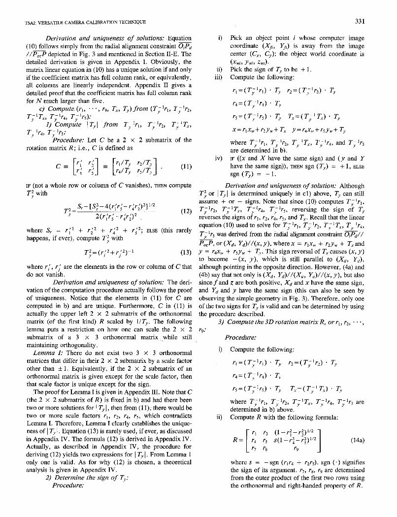
Derivation and uniqueness of solutions: Equation - (10) - follows simply from the radial alignment constraint 0;Pd //P,,P depicted in Fig. 3 and mentioned in Section 11-E. The detailed derivation is given in Appendix I. Obviously, the matrix linear equation in (10) has a unique solution if and only if the coefficient matrix has full column rank, or equivalently, all columns are linearly independent. Appendix I1 gives a detailed proof that the coefficient matrix has full column rank for N much larger than five.
c) Compute ( r l , * * * , r9, T,, T,) from (T;lr1, T;lr2, Ti'T,, T;lr4, T;lr5):
I ) Compute 1 Ty I from T; lrl, T;'r2, T;'T,, T; 'r4, T; 'r,:
Procedure: Let C be a 2 x 2 submatrix of the rotation matrix R ; i.e., C is defined as
IF (not a whole row or column of C vanishes), THEN compute T; with
where S, = r;2 + r i2 + r i 2 + r;2; ELSE (this rarely happens, if ever), compute T; with
T;=(r:2+rj2) -1 (13)
where r; , rj' are the elements in the row or column of C that do not vanish.
Derivation and uniqueness of solution: The deri- vation of the computation procedure actually follows the proof of uniqueness. Notice that the elements in (1 1 ) for C are computed in b) and are unique. Furthermore, C in ( 1 1 ) is actually the upper left 2 x 2 submatrix of the orthonormal matrix (of the first kind) R scaled by UT,. The following lemma puts a restriction on how one can scale the 2 X 2 submatrix of a 3 x 3 orthonormal matrix ,while still maintaining orthogonality.
Lemma I: There do not exist two 3 X 3 orthonormal matrices that differ in their 2 X 2 submatrix by a scale factor other than +. 1 . Equivalently, if the 2 X 2 submatrix of an orthonormal matrix is given except for the scale factor, then that scale factor is unique except for the sign.
The proof for Lemma I is given in Appendix 111. Note that C (the 2 X 2 submatrix of R ) is fixed in b) and had there been two or more solutions for I Ty 1, then from ( 1 l ) , there would be two or more scale factors r I , r2, r4, r5, which contradicts Lemma I. Therefore, Lemma I clearly establishes the unique- ness of I T, I. Equation (13) is rarely used, if ever, as discussed in Appendix IV. The formula (12) is derived in Appendix IV. Actually, as described in Appendix IV, the procedure for deriving (12) yields two expressions for I Ty I. From Lemma 1 only one is valid. As for why (12) is chosen, a theoretical analysis is given in Appendix IV.
2) Determine the sign of T,: Procedure:
i) Pick an object point i whose computer image coordinate (XB, Yfi) is away from the image center (C,, Cy); the object world coordinate is ( x w i , ~ w ; , 2 3 .
ii) Pick the sign of Ty to be + 1. iii) Compute the following:
r l=(T; l r l ) T, r2=(T,-'rz) + Ty
r4=(T;lr4) - Ty
r5=(T; 'r5) Ty T,=(T;lT,) T,
x=rlx,+r2yw+ T, y=r4x,+r5yw+T,
where Tilt-' , TY-'r2, T;'T,, T;'r4, and T;lr5 are determined in b).
iv) IF ( ( x and X have the same sign) and ( y and Y have the same sign)), THEN sgn ( T,) = + 1 , ELSE
sgn (T,) = - 1 .
Derivation and uniqueness of solution: Although T; or I Ty I is determined uniquely in cl) above, Ty can still assume + or - signs. Note that since (10) computes T; lrl, T;lr2, T;'T,, T;lr4, T;'r5, reversing the sign of Ty reverses the signs of r l , r2, r4, r,, and T,. Recall that the linear equation (10) used to solve for Ti l r l , T i1r2 , T i 'T , , T i1r4 , T i 'r5 was derived from the radial alignment constraint oiPd// PozP, or ( X d , Yd)//(& y ) , where x = rlxw + r2yw + T, and y = r4xw + r5y, + Ty . This sign reversal of Ty causes (x , y ) to become - ( x , y ) , which is still parallel to (Xdy Yd), although pointing in the opposite direction. However, (4a) and (4b) say that not only is (&, Yd)//(Xu, Y,)//(x, y ) , but also since f and z are both positive, and x have the same sign, and Yd and y have the same sign (this can also be seen by observing the simple geometry in Fig. 3 ) . Therefore, only one of the two signs for Ty is valid and can be determined by using the procedure described.
3) Compute the 3 0 rotation matrix R, or rl , r2, , r9 :
-
-
Procedure:
i) Compute the following:
r l=(T; l r1 ) Ty r2=(T;'rZ) Ty
r4= ( T;lr4) Ty
r5=(T;lr5) * Ty T,=(T;lT,) * Ty
where T;lrl, T;lr2, TiIT,, T;lr4, Ti1r5 are determined in b) above.
ii) Compute R with the following formula:
rl rz ( l - r : - r i )1 /2 R = r4 r5 s ( l - r ~ - r ~ ) 1 / 2 (144 [ r-i rx 1 r9
where s = - sgn (rlr4 + r2r5). sgn (e) signifies the sign of its argument. r7, rs, r9 are determined from the outer product of the first two rows using the orthonormal and right-handed property of R .

332 IEEE JOURNAL OF ROBOTICS AND AUTOMATION, VOL. RA-3, NO. 4, AUGUST 1987
iii) Compute the effective focal length f using (15) in d), to follow. IF ( f < 0), THEN
rl r2 - (1 -r;-r?j)l’2
R = [ r4 r5 -s(l-r:-rz)1’2 . (14b)
- r7 - r8 r9 1 Derivation and uniqueness of solution: Since
T;lrl, T;lr2, T;lr4, T;lr5 are uniquely determined in b) and T, is uniquely determined in c-1) and -2), obviously, rl, r2, r4, r5 are uniquely determined. Note that rl , r2 are the elements in the upper 2 X 2 submatrix of rotation matrix R. The problem becomes how to compute the rest of the elements uniquely in R. This is provided by the following lemma:
Lemma 2: Given 2 x 2 submatrix of a 3 x 3 orthonormal matrix of the first kind,2 there are exactly two possible solutions for the orthonormal matrix. They are given in (14a) and (14b).
Proof: The proof of Lemma 2 is given in Appendix V.
Now we explain why the procedure described earlier for choosing the one among (14a) and (14b) gives the correct and unique solution.
In (14a) and (14b), only the first two rows are given explicitly in terms of the given quantities rl , r2, r4, r5. From the orthonormal property of R and the right-handed rule (i.e., determinant of R is 1, not - l ) , r,, r8, and r9 are easily and uniquely computed from the first two rows. Only one among (14a) and (14b) is valid. This follows from the fact that by reversing the sign of z for all points in the camera 3D coordinate system, i.e., (x , y , z ) + (x, y , - z ) , all points are still coplanar (note that this is not permissible for noncoplanar points since the mirror image of object points with respect to z = 0 plane reverses the right-handed rule). However, since T, is not yet computed in stage 1, one cannot compute the z coordinate (= r7x, + r8yw + r9.0 + T,) yet. From (4a) and (4b), it is seen that reversing the sign of z also reverses the sign off. Therefore, the easiest way to select the valid one among the two solutions in (14a) and (14b) is to use the linear equation in d) below for computing approximation o f f and T, by ignoring distortion. The wrong one will yield negative f and the right one will yield positive f . Note that there is no need to worry about distortion just for deciding which among the two cases would yield positive f , since the actual quantity off is not needed for this purpose. This is always confirmed by the experimental results, as to be seen in Section IV.
2) Stage 2-Compute Effective Focal Length, Distor- tion Coefficients, and z Position:
d) Compute an approximation o f f and T, by ignoring lens distortion:
Procedure: For each calibration point i, establish the following linear equation with f and T, as unknowns:
[Y; - dy Yil [ ;,I = W d y Yi (1 5 )
Orthonormal matrix of the first kind, by definition, has determinant + 1, as opposed to orthonormal matrix of the second kind, whose determinant is - 1 .
where
y; = r4xwi + r5ywi + r6 * 0 + Ty
wi = r7xWi + rs ywi + r9 0.
With several object calibration points, this yields an overdeter- mined system of linear equations that can be solved for the unknowns f and T,. The calibration plane must not be exactly parallel to image plane, otherwise (15) becomes linearly dependent.
Derivation: Equation (15) is derived by setting K~ to zero in (8b). Since R, T,, and Ty have all been determined at this point, y and w are fixed. Thus (15) is a linear equation with f and T, as unknowns. Note that although (8a) can give rise to a similar equation, it is redundant. To solve for an approximation of f and T,, using (15), an overdetermined system of linear equation using a number of points can be established, and a least square solution is easily obtained. The proof for uniqueness off and T, can be found in Tsai [29].
e) Compute the exact solution f o r f , T,, K ~ :
Procedure: Solve (8b) with f , T,, K~ as unknowns using standard optimization scheme such as steepest descent. Use the approximation for f and T, computed in d) as initial guess, and zero as the initial guess for K ~ .
Derivation and uniqueness of solution: With R, T,, and Ty have all been determined previously, (8b) becomes a nonlinear equation with f , T,, K~ as unknowns. Usually only one or two iterations are needed.
G. Calibrating a Camera Using Monoview Noncoplanar Points
When s,, the uncertainty scale factor in X , is not known a priori, the calibration techniques using a noncoplanar set of calibration points should be used. The same pattern used in coplanar case can be used, except that it is moved to several different heights by a z stage. One can of course use a calibration pattern that is noncoplanar physically, but it is much easier to fabricate a coplanar set of calibration points than noncoplanar points whose image coordinates must be known accurately. Since zw is no longer identically zero, the linear matrix equation derived from the RAC yield solutions for seven unknowns instead of five, making both the computa- tion and proof of uniqueness in stage 1 less tricky than the coplanar case. Just like the monoview coplanar case, the origin for the object world coordinate system should be set up away from the origin and the y axis of the camera coordinate system. 1) Stage 1-Compute 3 0 Orientation, Position (x and
y ) and Scale Factor: a) Compute image coordinate ( X i , Y i ) , where ( X i ,
Y; ) is defined the same as the (Xd, Yd) in (6a) and (6b) except that s, is set to 1 (that is, the uncertainty scale factor is taken to be a perfect I):
Procedure: The procedure is the same as a) for stage 1 in Section 11-F except that s, is taken to be one. s, is absorbed into the unknowns for the linear equations in b) below and will be computed explicitly in c-3).

T;Ir4, T;lr5, T;lr6: Procedure: For each calibration point i with (xwi, ywi,
zwi) as the 3D world coordinate and (Xi i , Y&) as the modified image coordinate computed in a) above, set up the following linear equation with T - Isxrl, T; 's,r2, T; 'sXr3, T; 's,T,, TY-lr4, T; 'r5, and T; P r6 as unknowns:
[ YiiXw; YiiY, YiiZWi Yii -X&Xwi -x;;ywi -X;izwil
= X i i . (16)
With N (the number of object points) much larger than seven, an overdetermined system of linear equations can be estab- lished and solved for the seven unknowns T;'sxrl, T;ls,r2, T;IsXr3, T;'sxTx, T;lr4, T;lr5, and T;Ir6.
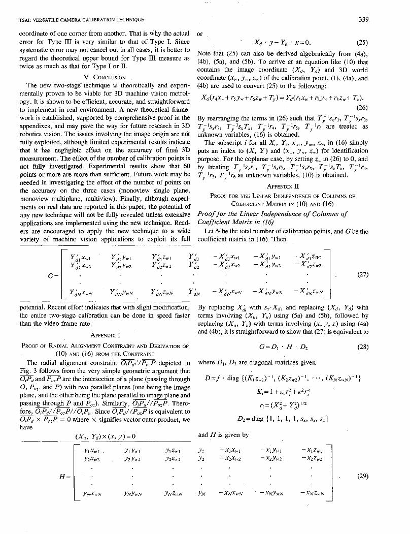
Derivation and uniqueness of solutions: Equation (16) is derived by following exactly the same procedure as coplanar case in using the radial alignment constraint but with zw not set to zero (see Appendix I for detail). Obviously, the matrix linear equation in (16) has a unique solution if and only if the coefficient matrix has full column rank, or equivalently, all columns are linearly independent: Appendix I1 contains a detailed proof that the coefficient matrix has full column rank for N much larger than seven.
e) Compute ( r l , + , rg, T,, Ty) from T;Isxr1, T;Isxr2, T; 's,r3, T;IsxTX, T; lr4, T;'r5, T;lr6: The derivation and proof of uniqueness of solution are straightfor- ward, and can be found in Tsai [29].
I ) Compute 1 Ty I from TJ1s,rl, T;'s,r2, T; ls,r3, T;'s,Tx, T;Ir4, T;lr5, T;lr6:
Procedure: Let ai, i = 1, * - - , 7 be defined as al = T; lsxrl, a2 = T-'sxr2, a3 = T; lsXr3, a4 = T;'s,T,, a5 = T; 'r4, a6 = T; c5, a7 = T; 'r6. Note that all the ai from i = 1, - * , 7 are determined in b). Compute I Ty I using the following formula:
2) Determine the sign of Ty: The procedure, deriva- tion, and uniqueness argument are the same as those for the coplanar case.
3) Determine s,: Procedure: Use the following formula to compute
S, :
sx=(a~+a~+a:)1 '21 Tyl . (18)
4) Compute the 3 0 rotation matrix R, or r l , r2, * ,
Procedure: Compute rl, r2, r3, r4, r5, r6, and T, rg :
with the following formula:
rl = a1 - Ty/s, r2= a2 Ty/s, r3 = a3 Ty/s,
r4= a5 . Ty r5 = a6 Ty r6= a7 _ * Ty
T,=u~ * Ty
where ai, i = 1, e , 7 are defined in (1) and are the seven variables computed in b).
Given r;, i = 1, - + , 6, which are the elements in the first two rows of R, the third row of R can be computed as the cross product of the first two rows, using the orthonormal property of R and the right-handed rule (determinant of R = 1, not - 1).
Derivation and uniqueness: The derivation simply follows from the definition of ai in b). The uniqueness follows from the fact that the formula is explicit and that given two rows of a 3 x 3 orthonormal matrix with determinant + 1, the third row is always unique.
2) Stage 2-Compute Effective Focal Length, Distor- tion Coefficients, and z Position:
a) Compute of an approximation of f and Tz by ignoring lens distortion: The procedure, derivation, and uniqueness are exactly the same as that for the coplanar case.
b) Compute the exact solution for f, T,, K ' : This again is the same as the coplanar case.
H. Multiple Viewing Position Calibration When more than one view is taken at different position and
orientation relative to the calibration points with a single camera, the extrinsic parameters of the camera differs from view to view, but the intrinsic parameters remain the same. We can exploit this when using multiple views by choosing the set of intrinsic parameters that optimizes the global consist- ency between camera model and observations. The disadvan- tage that quickly comes to mind is the increase of dimensional- ity in parameter space, making the computation less suitable for automated robotics application. However, because the new two stage technique computes most of the extrinsic parameters in stage 1, the disadvantage of increase in dimensionality for parameter space no longer prevails. Due to the limit of space, the technique using multiple view is not described here. See Tsai [29] for detail.
111. ACCURACY ASSESSMENT
It is difficult to obtain high accuracy ground truth for camera calibration parameters that can serve as absolute reference. Therefore, we will assess the accuracy of the two- stage camera calibration by how well it can sense or measure the 3D world.
A . Three Types of Measures for Camera Calibration Accuracy
We will adopt the following three types of measures. Type I-Accuracy of 3 0 Coordinate Measurement
Obtained through Stereo Triangulation Using the Cali- brated Camera Parameters: The procedure is as follows.
1) Calibrate one camera using either coplanar or nonco- planar points, monoview or multiview. If monoview calibra- tion is used, repeat the calibration procedure for another camera rigidly connected with camera 1 (the purpose of the

334 IEEE JOURNAL OF ROBOTICS AND AUTOMATION, VOL. RA-3, NO. 4, AUGUST 1987
second camera is to provide stereo triangulation capability to be used later).
2) Acquire 2D image coordinates for a set of test points whose 3D coordinates are known relative to the same 3D world coordinate system used for the calibration points, using the camera (or cameras) in the same viewing position as for the calibration.
3) Compute the 3D coordinates of the above test points in the world coordinate system using stereo triangulation. If multiview calibration was used, two views are sufficient for stereo triangulation. If monoview calibration was used, then since two cameras rigidly connected together in (1) were calibrated, stereo triangulation can still be done.
4) The accuracy of camera calibration is assessed by comparing the difference between the known 3D coordinates of the test points and the coordinates computed in (3). That comparison can be done either in the 3D world coordinate system, or in the computed 3D camera coordinate system. We will use the latter throughout this section because in 3D camera coordinate system, physical meaning can be easily attached to the x, y , z coordinates. For example, z coordinate is the depth, and x and y coordinate axes are parallel to X, Y coordinate axes in the image plane.
Type 11-Radius of Ambiguity Zone in Ray Tracing: As shown in Fig. 1, the calibration process tries to find
camera model parameters such that the ray starting from the optical center 0, passing through the true image point Pd (the ray bends at Pd according to the extent of radial distortion), will eventually pass through the calibration object point P. Of course, due to error, the ray will not exactly pass through P. After the camera model is calibrated or reconstructed, this path of ray in Fig. 1 can be back traced, that is, starting from the optical center, the ray can be traced through the image point and “back projected” into the object world passing through the object point P. One way of measuring the camera calibration accuracy is the extent of ambiguity of error of this ray tracing in one view, which is the basis of Type I1 measure. As seen in Fig. 5 , error of camera model reconstruction causes the ray to miss the point P. Using Type I1 measure in assessing camera calibration accuracy is to see how much the ray misses the object point P. To see the relationship between Type I1 and I measures, consider the fact that if the ray tracing can be done very accurately, then obviously with two views, the intersec- tion of the two rays gives the 3D coordinate of the object point P. Therefore, the accuracy of reconstructing the 3D coordi- nate of P is a measure of the accuracy of camera calibration, which is the basis for the Type I measure just described. The procedure is as follows.
1) Calibrate the camera using a coplanar set of points on a plane (called plane V in Fig. 5 ) .
2) Set up a coplanar set of test points whose 3D coordinates in the object world coordinate system (in which the coordinate of the calibration points are defined) are known, and the position of the plane (called plane U in Fig. 5) on which the test points reside is also known. Take one view.
3) For each image point Pd on the test plane U, use the calibrated camera model in (1) to back project the ray from 0 through Pd and intersect with plane U at P’ . The distance
Fig. 5. Radius of ambiguity zone is Type 11 measure for camera calibration accuracy, P is ideal object point, and P’ is point where back projected ray using calibrated camera model intersects with object surface plane U.
between P’ and P (the ideal point in plane U ) is called the radius of the ambiguity zone (as depicted in Fig. 5) .
Type 111-Accuracy of 3 0 Measurement: Since a cali- brated camera may be applied to measure relative 3D information instead of absolute 3D coordinate, e.g., dimen- sional inspection of mechanical parts, it is useful to measure the goodness of camera calibration by how well the camera can be used to perform dimensional measurement.
B. Accuracy Analysis Summary As explained earlier in this section, we assess the accuracy
of camera calibration by measuring how accurately the camera measures the 3D world. The remainder of this section reviews the formula of accuracy or error for camera calibratiod3D measurement provided in Tsai [26] which will later be used for the analysis of experimental results. It is important to note that the purpose of this section is not to propose a new accuracy results or to prove its validity. The accuracy analysis formula is only to double check the numerical figures of the experi-, mental results.
C. Theoretical Upper Bound of Error for 3 0 Measurement
It is shown in Tsai [26] that the error of 3D measurement of the x, y , z coordinate of a feature point using stereo triangulation is bounded above by
1 1 Z +- +--I - * 6 + A q (22) 2- 2 a . f II Gll
where
6 effective image spatial quantization or the error of
TSAI: VERSATILE CAMERA CALIBRATION TECHNIQUE 335
estimated image feature location (see more discus- sion about 6 in the following),
No total number of points used in calibration, 11 T,ll distance between the optical centers of the two
camera viewing stations, Nf number of views used in calibration (i.e., one for
monoview calibration, two for multiple viewing position calibration using two views, etc.),
L dimension of the image sensor chip, or more generally the size of the active area in image plane scanned by the camera,
A q target ambiguity in three-space (e.g., if the corner of a rectangular block is the target point, then the edge break or the sharpness of edges determines the extent of ambiguity for the true location of the target point).
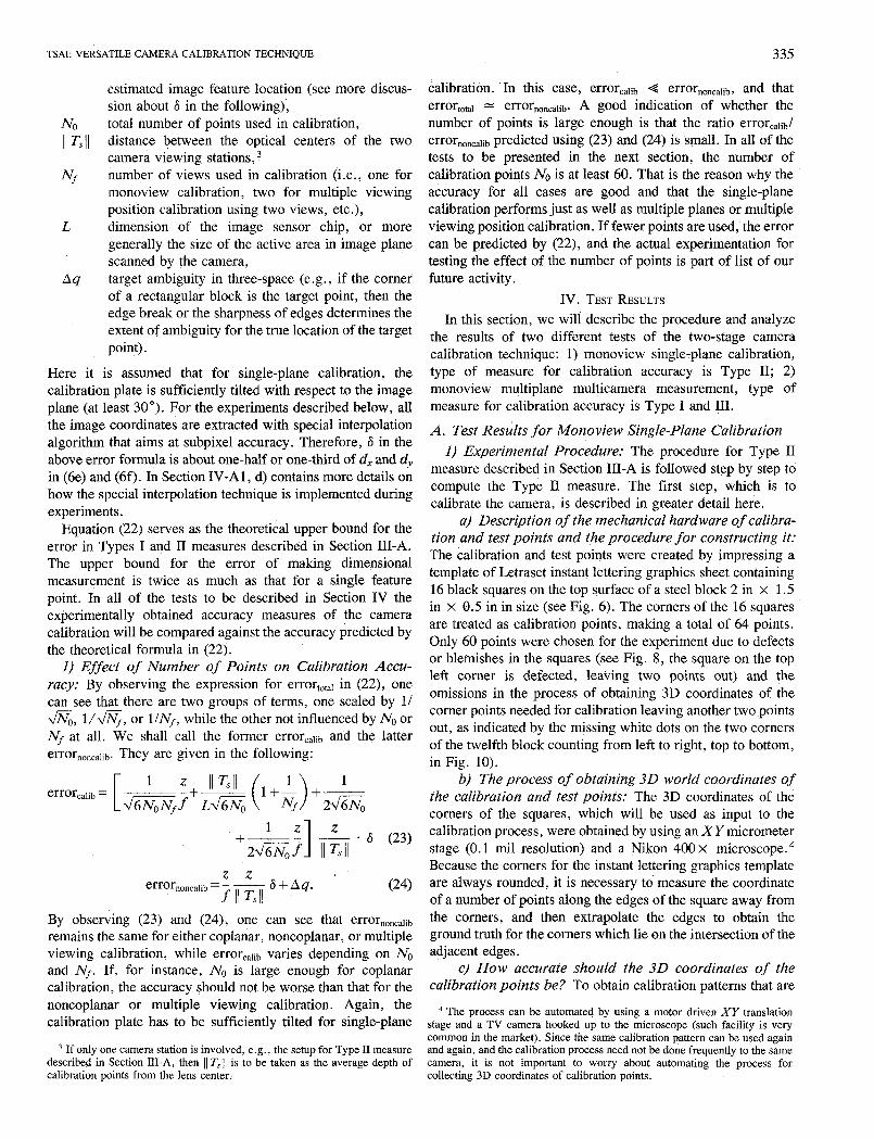
Here it is assumed that for single-plane calibration, the calibration plate is sufficiently tilted with respect to the image plane (at least 30"). For the experiments described below, all the image coordinates are extracted with special interpolation algorithm that aims at subpixel accuracy. Therefore, 6 in the above error formula is about one-half or one-third of d, and dy in (6e) and (6f). In Section IV-A1, d) contains more details on how the special interpolation technique is implemented during experiments.
Equation (22) serves as the theoretical upper bound for the error in Types I and I1 measures described in Section 111-A. The upper bound for the error of making dimensional measurement is twice as much as that for a single feature point. In all of the tests to be described in Section IV the experimentally obtained accuracy measures of the camera calibration will be compared against the accuracy predicted by the theoretical formula in (22).
I ) Effect of Number of Points on Calibration Accu- racy: By observing the expression for errortotal in (22), one can see that there are two groups of terms, one scaled by 1/ fro, l/*, or 1/Nf, while the other not influenced by NO or Nf at all. We shall call the former errorcalib and the latter errornoncalib. They are given in the following:
+--I 1 - z * 6 (23)
2m.f II T.11 z z
errornoncalib = - - f I1 Tsll 6 + A q .
By observing (23) and (24), one can see that errornoncalib remains the same for either coplanar, noncoplanar, or multiple viewing calibration, while errorcalib varies depending on NO and NJ. If, for instance, No is large enough for coplanar calibration, the accuracy should not be worse than that for the noncoplanar or multiple viewing calibration. Again, the calibration plate has to be sufficiently tilted for single-plane
If only one camera station is involved, e.g., the setup for Type I1 measure described in Section 111-A, then 11 T,/i is to be taken as the average depth of calibration points from the lens center.
calibration. In this case, errorcalib 4 errornoncalib, and that errortoal = errorno,,,lib. A good indication of whether the number of points is large enough is that the ratio errorcalib/ errornoncalib predicted using (23) and (24) is small. In all of the tests to be presented in the next section, the number of calibration points NO is at least 60. That is the reason why the accuracy for all cases are good and that the single-plane calibration performs just as well as multiple planes or multiple viewing position'calibration. If fewer points are used, the error can be predicted by (22), and the actual experimentation for testing the effect of the number of points is part of list of our' future activity.
IV. TEST RESULTS In this section, we will describe the procedure and analyze
the results of two different tests of the two-stage camera calibration technique: 1) monoview single-plane calibration, type of measure for calibration accuracy is Type 11; 2) monoview multiplane multicamera measurement, type of measure for calibration accuracy is Type I and 111.
A. Test Results for Monoview Single-Plane Calibration 1) Experimental Procedure: The procedure for Type I1
measure described in Section 111-A is followed step by step to compute the Type I1 measure. The first step, which is to calibrate the camera, is described in greater detail here.
a) Description of the mechanical hardware of calibra- tion and test points and the procedure for constructing it: The calibration and test points were created by impressing a template of Letraset instant lettering graphics sheet containing 16 black squares on the top surface of a steel block 2 in X 1.5 in X 0.5 in in size (see Fig. 6). The corners of the 16 squares are treated as calibration points, making a total of 64 points. Only 60 points were chosen for the experiment due to defects or blemishes in the squares (see Fig. 8, the square on the top left corner is defected, leaving two points out) and the omissions in the process of obtaining 3D coordinates of the corner points needed for calibration leaving another two points out, as indicated by the missing white dots on the two corners of the twelfth block counting from left to right, top to bottom, in Fig. 10).
b) The process of obtaining 3 0 world coordinates of the calibration and test points: The 3D coordinates of the corners of the squares, which will be used as input to the calibration process, were obtained by using an X Y micrometer stage (0.1 mil resolution) and a Nikon 400 x micro~cope.~ Because the corners for the instant lettering graphics template are always rounded, it is necessary to measure the coordinate of a number of points along the edges of the square away from the corners, and then extrapolate the edges to obtain the ground truth for the corners which lie on the intersection of the adjacent edges.
e) How accurate should the 3 0 coordinates of the calibration points be? To obtain calibration patterns'that are
The process can be automated by using a motor driven X Y translation stage and a TV camera hooked up to the microscope (such facility is very common in the market). Since the same calibration pattern can be used again and again, and the calibration process need not be done frequently to the same camera, it is not important to worry about automating the process for collecting 3D coordinates of calibration points.

336 IEEE JOURNAL OF ROBOTICS AND AUTOMATION, VOL. RA-3, NO. 4, AUGUST 1987
Fig. 6 . Steel block on top of which Letraset instant lettering graphics are impressed. Corners of black squares are calibration points.
highly accurate and easily processed by the computer is not easy. Therefore, one should consider how accurate the calibration points must be to achieve a certain accuracy for calibratiod3D measurement. Note that errorcalibration in (23) is scaled by -I. Therefore, for a large number of points, errorcalibration becomes negligible compared with er- rornoncalibration. However, (23) assumes that the error of calibra- tion points is either comparable to image spatial quantization error and random, or is much less than image spatial quantization error irrespective of randomness. Therefore, if there is any factor during the process of creating and measuring the 3D coordinates of the calibration points that would cause the error of calibration coordinates to be nonrandom or systematic, that factor must be reduced to a minimum such that the nonrandom error is less than the desired final accuracy of 3D measurement. If the desired measurement accuracy is of the order of 1 mil, then the factors such as flatness of the surface holding the calibration pattern and the parallelism between the top and bottom of the surfaces are the only factors that need to be controlled. All other factors tend to give random error and can easily be made smaller than image spatial quantization. It is important to keep the tolerance for the flatness and parallelism at least one order of magnitude tighter than the final goal of 3D measurement using the calibrated camera; for example, if the find accuracy is desired to be 1 mil, then the surface flatness and parallelism has to be 0.1 mil accurate.
d) Extraction of computer image coordinates for the calibration and test points: Images of calibration and test objects were acquired with a Fairchild CCD 3000 camera and a Fuji 25-mm focal length TV lens, using the setup shown in Fig. 7. The objects were illuminated using a fiber-optic illuminator (any intense diffuse source would also work).
Computer image coordinates for calibration and test points (corners of black Letraset squares) were extracted as follows.
1) Acquire a gray scale image (see Fig. 8). 2) Threshold the image to produce a binary image (see Fig.
9); the exact threshold value is not critical and could be set by analysis of intensity histograms or some ad hoc method (in the current work, the threshold was selected manually).
Fig. 7. Setup for camera calibration for all tests. Only one of two cameras is used for first two tests.
Fig, 8. Gray scale image of calibration pattern viewed by computer. One square is defective.
Fig. 9. Thresholded binary image of calibration pattern viewed by com- puter.

TSAI: VERSATILE CAMERA CALIBRATION TECHNIQUE
Fig. 10. White dots at corners of black squares are calibration points extracted by computer using special interpolation technique, which reduces effect of image spatial quantization of factor of 2 or 3.
Link edge points in the binary image to extract a set of approximate boundary edges. Scan in the direction perpendicular to the approximate edge locations in the gray scale image to locate the “true” edge points using interpolation. Fit straight lines to true edge points. Then compute intersections, yielding feature point (corner) coordi- nates. Fig. 10 illustrates the result by superimposing white dots on the original gray scale image at computed feature locations. This procedure yielded image coordi- nates with an accuracy of 1/2 to 1/3 pixel; in the CCD 3000 camera, pixels .are spaced approximately 1 mil apart (center to center, in X and Y directions).
e) Compute camera intrinsic and extrinsic parameters using the two-stage technique: With the image coordinates extracted in d) and the 3D world coordinates of the calibration points obtained in b), the key equations (lo), (15), and (8b) used for camera calibration can be used if s, is given. A priori knowledge of s, is needed only for single plane case. Since our experience shows that s, is quite consistent for CCD 3000 camera, the same s, can be used for any Fairchild 3000 camera. Furthermore, in many cases, when one changes the lens and/or exterior orientation/position of the camera, the calibration must be done again, but s, is already calibrated before. We simply take the value of s, that we normally find for Fairchild CCD 3000, which is 1.042, in this experiment. It is found that with Fuji 25-mm lens, the angle is wide enough so that the radial distortion is significant. The distortion is found to be barrel type negative distortion, as expected. The undistorted image coordinate (Xu, Y,) computed from com- puter image coordinate (X, Y ) and the calibrated distortion coefficients K ~ , ~2 are displayed in Fig. 11, together with the original distorted points. For the points far away from the center, the distortion is about three to four pixels.
2) Experimental Results for Monoview Single-Plane Calibration: A total of 60 calibration points and 60 test points were used, and Type I1 measure described in Section 111-A is
337
computed and tabulated below. Type I1 measure:
Average radius of ambiguity zone 0.7 mil Maximum radius of ambiguity zone 1.3 mil
-______-
-
Note: 1 mil = 0.001 in. The computer time for calibration is 1.5 s. This computer
time refers to the time taken for performing steps 1 and 2 of the calibration procedure. It can be reduced to half a second when seven calibration points are used. The program is not optimized for speed performance. It can further be reduced if effort is invested to optimize the program. The computer used is a 68 000 based MASSCOMP minicomputer. We have very recently improved the speed such that it only takes 20 ms to do extrinsic calibration and less than 1 s to do the whole calibration when 36 points are used. It is expected to improve even more. In fact with slight modification, the entire two- stage calibration can be done in less than 30 ms.
In the above test, the image origin is chosen to be the apparent center of the sampled image (see the discussion and derivation of a) in Stage 1 of Section I-F. Experiments were also conducted using an arbitrarily chosen image origin (10 X 10 off the origin used in the above test); the results show no significant difference (see discussion and derivation of a) in Stage 1 of Section I-F.
3) Analysis: a) Comparison between experimentally obtained er-
ror and predicted error: To use (22)-(24) to obtain a theoretical upper bound on error, the following parameters are necessary:
L = 0.4 in f-1.1 in 2-4 in Ts=3 in
Aqz0.1 mil Nf= 1 d,= dy - 1 mil
No(number of points) = 60.
Since super resolution interpolation scheme was used when extracting image coordinates, the effective image spatial quantization 6 is about 1/2 or 1/3 of d, or dy , the distance between adjacent CCD sensor elements. Using (22)-(24), the following table for the theoretical upper bound of three types of error described in Section 111-B is obtained.
Effective image quantization 6 = 112 mil 6 = 113 mil Errortolal (predicted) 3.3 mil 2.3 mil
It is clearly seen by comparing the order of magnitude between the theoretical error bound and the actual error, the error bound is tight enough.
b) Predicted effect of number of calibration points: In Section 111-C1 it is explained why the ratio errorcalib/ error,,,,lib gives a good indication or theoretical prediction of whether the number of points is large enough. From (23) and (24), the following table is obtained:
______
Effective Image Quantization 6 = 112 mil 6 = 113 mil
Error,,,,, 0.7 mil 0.5 mil
ErrOr,,lib/errOr,,,calih 29 percent 28 percent ErrOrnoncd>h 2.5 mil 1.7 mil
______

338 IEEE JOURNAL OF ROBOTICS AND AUTOMATION, VOL. RA-3, NO. 4, AUGUST 1987
Fig. 11. White dots near corners of black square are original calibration points and corrected or undistorted points. Size of frame buffer holding image is 480 x 512. Therefore, it is seen that distortion near border is roughly three to four percent.
Since the ratio is small, it can be inferred that increasing the number of calibration points will not reduce the error measure for calibration significantly. This is the reason why the accuracy obtained in this case is not worse than that for the noncoplanar and multiple viewing calibration to be described later.
B. Test Results for Monoview Multiple-Plane Multicamera Measurement
I ) Experimental Procedure: The procedure is exactly the same as that for the previous test (coplanar case) except that a Klinger vertical micrometer stage is used to move the steel block to eight different heights and eight views are taken without moving the camera. However, instead of computing Type II measure, Types I and ID are to be computed. For this reason, the second camera in Fig. 7 is needed. The image coordinates extracted from the eight views are collected together and treated as if they were taken from one single view of eight planes of calibration points. The total height variation is only about 0.18 in, because the depth of focus and the total travel range of the vertical stage are limited. Nevertheless, the experimental results indicate that the extra depth information was good enough to estimate all the intrinsic and extrinsic parameters (including s,) with good accuracy, as can be seen in the following report of experimental results. The calibration done to one of the cameras as in the previous test is repeated identically to the second camera. Then a new set of test points (60 in total) whose 3D world coordinates are measured in advance are viewed by both cameras. Then stereo triangula- tion is used to compute Type I and I11 measure.
2) Experimental Results for Monoview Multiple-Plane Calibration:
~ ~ ~ _ _
Type I Measure Type 111 Measure ~-~
X Y distance between coordinate coordinate depth corners of square
Average error 0.4 mil 0.3 mil 0.6 mil 0.5 mil Maximum error 1.3 mil 1.5 mil 1.8 mil 1.4 mil _ _ _ _ ~ --
The total range of x, y are the size of the calibration pattern (1 in X 1 in), and the total range of depth in the camera coordinate system is about from 4 in to 4.5 in. Since eight planes were used, the computer time for calibration is 9 s. However, only two or three planes are actually needed. That time should be reduced by a factor of five. Also, on each plane, 60 points were used. Another factor of ten can be reduced in the computer time if only seven points are used on each plane, When fewer points are used, the accuracy degrades somewhat, but not much. Since complete camera calibration need not be done every millisecond, using 60 points give great accuracy with good speed. However, we will investigate the real benefit of reducing the number of points in the future.
3) Analysis: The experimental setup and parameters are identical to that in the previous test. The only difference is the type of measure used to assess the camera calibration accuracy. Since same error formula applies both to measures Type I and Type 11, the theoretical error as well as the analysis is identical to that of the previous test. Notice that the actual error for type 111 measure is similar to that for Type I . According to Section 111-B the upper bound for measurement of dimension theoretically should be twice as much as that for a single point feature. However, in measuring dimension, such as distance between corners of a square, certain systematic error sometimes cancels out when one subtracts the 3D
TSAI: VERSATILE CAMERA CALIBRATION TECHNIQUE
coordinate of one corner from another. That is why the actual error for Type 111 is very similar to that of Type I. Since systematic error may not cancel out in all cases, it is better to regard the theoretical upper bound for Type 111 measure as twice as much as that for Type I or 11.
V. CONCLUSION The new two-stage- technique is theoretically and experi-
mentally proven to be viable for 3D machine vision metrol- ogy. It is shown to be efficient, accurate, and straightforward to implement in real environment. A new theoretical frarne- work is established, supported by comprehensive proof in the appendixes, and may pave the way for future research in 3D robotics vision. The issues involving the image origin are not fully exploited, although limited experimental results indicate that it has negligible effect on the accuracy of final 3D measurement. The effect of the number of calibration points is not fully investigated. Experimental results show that 60 points or more are more than sufficient. Future work may be needed in investigating the effect of the number of points on the accuracy on the three cases (monoview single plane, monoview multiplane, multiview). Finally, although experi- ments on real data are reported in this paper, the potential of any new technique will not be fully revealed unless extensive applications are implemented using the new technique. Read- ers are encouraged to apply the new technique to a wide variety of machine vision applications to exploit its full
r
339
or Xd ' y - Yd ' x=o. (25)
Note that (25) can also be derived algebraically from (4a), (4b), @a), and (5b). To arrive at an equation like (10) that contains the image coordinate (Xd , Yd) and 3D world coordinate (xw, yw, z,) of the calibration point, (l), (4a), and (4b) are used to convert (25) to the following:
xd(r4xw+r5Yw+r6~w+ T,)= Y d ( r l ~ , + r 2 ~ ~ f r 3 z ~ + T,). (26)
By rearranging the terms in (26) such that T i lsXrl, T; 's,r2, T,-IsXr3, T; 's,Tx, T;lr4, T; 'rS, T;lr6 are treated as unknown variables, (16) is obtained.
The subscript i for all Xi , Yi, x,!, ywi, zwi in (16) simply puts an index to ( X , Y ) and (xw, y,, z,) for identification purpose. For the coplanar case, by setting zw in (26) to 0, and by treating T i lsxr1, T; ls,r2, T; Is,r3, T i 's,T,, T; lr4; T; 'r5, T i 'r6 as unknown variables, (10) is obtained.
APPENDIX I1 PRWF FOR THE LINEAR INDEPENDENCE OF COLUMNS OF
COEFFICIENT MATRIX IN (10) AND (16) Proof for the Linear Independence of Columns of Coefficient Matrix in (16)
coefficient matrix in (1 6). 'Then Let N be the total number of calibration points, and G be the
1
L
potential. Recent effort indicates that with slight modification, the entire two-stage calibration can be done in speed faster than the video frame rate.
APPENDIX I PROOF OF RADIAL ALIGNMENT CONSTRAINT AND DERIVATION OF
(10) AND (16) FROM THE CONSTRAINT The radial alignment constraint oiPd//Po,P depicted in
Fig. 3 follows from the very simple geometric argument that OiPd and P,,P are the intersection of a plane (passing through 0, Po,, and P ) with two parallel planes (one being the image plane, and the other being the plane parallel to image plane and passing through P and Poz). Similarly, OiP,//P,,P. There- fore, o i ~ d / / P o , ~ / / o ; P , . Since oipd//p,$ is equivalent to oipd x PozP = 0 where x signifies vector outer product, we have
__-
- -
- - - - - - -
__-
( x d ? yd) x (x, Y>=O
H =
- Y l X W I YlYWl Y l Z W l
Y 2 X w 2 Y 2 Y w 2 Y 2 Z W 2
YNXWN YNYWN YNZWN -
A
By replacing Xii with s,-Xd, and replacing (Xd, Yd) with terms involving (X,, Y,) using (5a) and (5b), followed by replacing (X,, Y,) with terms involving ( x , y , z ) using (4a) and (4b), it is straightforward to show that (27) is equivalent to
G=D1 H * 0 2 (28)
where Dl , D2 are diagonal matrices given
D=f - diag {(KIZ~I)-~, (K2zw2)V1, ( K N Z ~ N ) - ' }
Kj= 1 + f K2rf
ri= ( X i + Y$)1'2
D2=diag (1, 1, 1, 1, s,, s,, s,}
and H is given by
YI - X I X w l - X I Y w l -XIZWl
Y2 -x2xw2 - X 2 Y w 2 - x2zw2
. , YN - X N X W N - XNYWN - X N Z W N
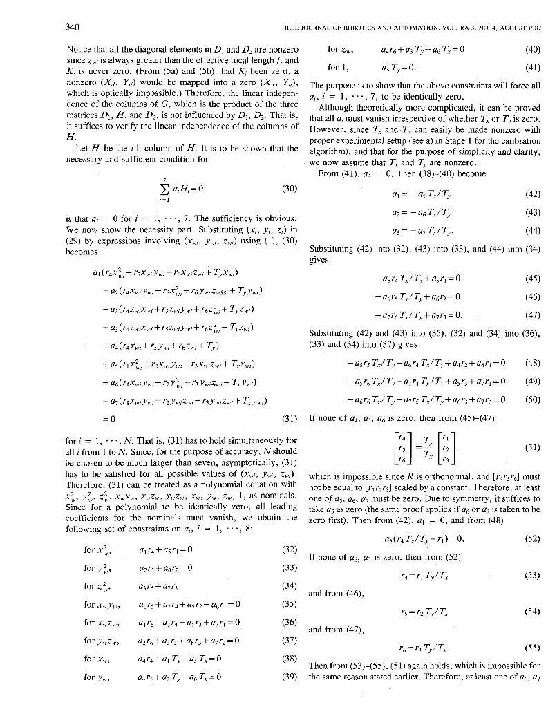
340 IEEE JOURNAL OF ROBOTICS AND AUTOMATION, VOL. RA-3, NO. 4, AUGUST 1987
Notice that all the diagonal elements in Dl and D2 are nonzero since zwi is always greater than the effective focal lengthf, and Ki is never zero. (From (5a) and (5b), had Ki been zero, a nonzero (X,, Y,) would be mapped into a zero (Xu , Yu), which is optically impossible.) Therefore, the linear indepen- dence of the columns of G , which is the product of the three matrices D l , H , and 4 , is not influenced by Dl , D2. That is, it suffices to verify the linear independence of the columns of H.
Let Hi be the ith column of H. It is to be shown that the necessary and sufficient condition for
The purpose is to show that the above constraints will force all a;, i = 1, . . . , 7, to be identically zero.
Although theoretically more complicated, it can be proved that all ai must vanish irrespective of whether T, or Ty is zero. However, since T, and Ty can easily be made nonzero with proper experimental setup (see a) in Stage 1 for the calibration algorithm), and that for the purpose of simplicity and clarity, we now assume that T, and Ty are nonzero.
From (41), a4 = 0. Then (38)-(40) become
a1 = -
U2 = - U6 Tx/ Ty (43) is that ai = 0 for i = 1, . . a , 7. The sufficiency is obvious. We now show the necessity part. Substituting (xi, yi, zi) in a3 = - a7 Tx/Ty. (44) (29) by expressions involving (xwi, ywi, zwi) using (11, (30) becomes Substituting (42) into (32), (43) into (33), and (44) into (34)
gives
for i = 1, , N. That is, (3 1) has to hold simultaneously for all i from 1 to N. Since, for the purpose of accuracy, N should be chosen to be much larger than seven, asymptotically, (31) has to be satisfied for all possible values of (xwi, ywir zwi). Therefore, (31) can be treated as a polynomial equation with
Y:, z2,, xWyw, x,zw, yWz,, xu,, yw, z,, 1, as nominals. Since for a polynomial to be identically zero, all leading coefficients for the nominals must vanish, we obtain the following set of constraints on a;, i = 1, . . e , 8:
for x;, alr4+u5r1=0 (32)
for Y ”,, a2r5 + a6r2 = 0 (33)
for zt, a3 r6 + a7 r3 (34)
forxIYyW, a l rS+a2r4+a5r~+a~r l=0 (35)
for xwzw, alr6+a3r4+a5r3+a7rl=0 (36)
foryWzw, azr6+a3r5+a6r3+a7r2=0 (37)
[ I r6 =g [;I which is impossible since R is orthonormal, and [r4r5r6] must not be equal to [rlr2r3] scaled by a constant. Therefore, at least one of a5, a6, a7 must be zero. Due to symmetry, it suffices to take as as zero (the same proof applies if 0 6 or a7 is taken to be zero first). Then from (42), a1 = 0 , and from (48)
U6(T4T,/Ty-rl)=0. (52)
If none of a6, a7 is zero, then from (52)
r4 = rl Ty/T, (53)
and from (46),
r5 = r2 Ty / T, (54)
and from (47),
r, = r3 TJT,. (55 ) for x,, a4r4+al Ty+a5 T,=O
for yw, a4r5+a2Ty+a6T,=0
(38) Then from (53)-(55), (51) again holds, which is impossible for (39) the same reason stated earlier. Therefore, at least one of 0 6 , a7

TSAI: VERSATILE CAMERA CALIBRATION TECHNIQUE 34 1
must vanish. Again, for symmetry and simplicity, we take a6 to be zero. Then from (43) a2 = 0. From (49)
a7(rlr4 Tx/T,) = O . (56)
From (50),
a7(r2rs Tx/T,)=O. (57)
If, at this point, a7 is not zero, then from (47)
r3 = r6 Tx/ T,
from (56), rl = r4 Tx/T,
from (57), r2 = rs Tx/ Ty
which implies that
Proofi Let R be defined as a 3 X 3 orthonormal matrix defined in (2), and let R2 be the 2 X 2 submatrix of R :
The purpose is to show that there is no way one can construct a 3 X 3 orthonormal matrix from a 2 X 2 submatrix
c = s * [;; ;] with s different from t 1 . Since orthonormality is maintained no matter how the rows and columns are permuted, we assume that the 2 x 2 submatrices are in the upper left corner of the 3 x 3 orthonomal matrices. Let R and Re be 3 x 3 orthonormal matrices constructed from R2 and C. Then from the fact that the norm of each row and column of R is unity (without yet considering orthogonality), R must assume the following form:
rl r2 k(1 - r f - r i ) 1 / 2 R = [ r4 r5 t ( l - r : - r : )1 /2
t ( 1 - r: - r ! ) f ( l - r i - r : ) 1 / 2 f ( - 1 + S,)’/2
and is impossible. Thus a7 must vanish, which also implies where S, = r f + r i + ri + r:. from (44) that a3 = 0. In conclusion, the necessary and Similarly, if R, exists, it must assume the following form sufficient condition for (30) is that ai = 0 for i = 1 , * * * , 7 . (using the property of unity row and column norm only)
ST1 sr2 t [ l - ~ ~ ( r f - r i ) ] I / ~ Re= [ sr4 sr5 -t [ l - ~ ~ ( r i - r ; ) ] l / ~ . 1 (59)
t [ l - ~ ~ ( r f - - r ; ) ] ’ / ~ f [ l - ~ ~ ( r i - r : ) ] I ’ ~ f (- 1 +s2Sr)”2
Proof for the Linear Independence of Columns of Coefficient Matrix in (IO)
The only differences between coefficient matrix in (10) and in (16) are that ( X d , Y d ) is used in ( lo ) , while ( X ; , Y i ) = ( S x X d , Y d ) is used in (16), and that the column space of (10) is part of the column space in (16) (the third and seventh columns are missing (10)). By setting D2 in (28) to an identity matrix, which takes care of the first difference, and by considering the fact that the subspace of a linearly independent column space is always linearly independent, the coefficient matrix in (10) also has linearly independent columns. This completes the proof.
APPENDIX I11
PROOF OF LEMMA 1
Lemma I : There do not exist two 3 x 3 orthonormal matrices that differ in their 2 x 2 submatrix by a scale factor other than +. 1 . Equivalently, if the 2 x 2 submatrix of a 3 x 3 orthonormal matrix is given except for the scale factor, then that scale factor is unique except for the sign.
In the following, it is to be shown that with the orthogonality condition imposed, s is forced to take the values of & 1 only.
Since the first two columns of R are mutually orthogonal, we have
r1r2+r4rs= * ( I -rf-r:)Il2(1 -ri-r:)II2. (60)
Similarly, for Re,
s2(rlr2+r4rs)= k [ 1 - s 2 ( r ~ + r ~ ) ] ~ ~ z [ l - s z ( r ~ + r ~ ) ] . (61)
By substituting rlr2 + r4rs in (61) with the right-hand side of (60), (61) becomes
( 1 - ~ ~ s 4 + ~ ~ 9 - 1 = 0
or
[ ( l - Sr)s2+ ll(s2- 1) = 0. (62)
From (62), s2 can assume two possible values:
s2= 1 (63)

342
or
IEEE JOURNAL OF ROBOTICS AND AUTOMATION, VOL. RP-3, NO. 4, AUGUST 1987
Now we show that (64) is valid and is equivalent to (63). Observe that r9 (the (3, 3)th element) in (58)) is k ( - 1 + Sr)lI2. Since lr91 I 1 , we have
- 1 + S , I 1 . (65)
Let the (3, 3)th element of R, be denoted as rC9. Substituting (64) into the expression for rC9 in (59) gives
rC9= f 1 -- ( s,: 1 >,I2
=i(> 1 1/2 . s,- 1
Since lrC9l I 1, I/($ - 1 ) I 1, or
From (65) and (66) S, - 1 = 1 . Thus (64) becomes
and
From Lemma 1, I Ty I of T; is unique. Thus only one among (71a) and (71b) is valid. We now prove that only (71a) or (12) is valid. Substituting (70) into expression for r9 in (69) gives
r9= f [ T;?(r,'r;-r;r;)2]1/2. (71)
Thus from (71)
Substituting (71b) into (72) gives
After some simple algebraic manipulation, the following is derived:
However, from triangular inequality, Thus s = + 1 . This completes the proof.
APPENDIX IV
DERIVATION OF COMPUTATION PROCEDURE FOR Ty
Case I: Not a Whole Row or Column of C Vanishes
From the definition of C and r ,' , ri , r i , r; in ( 1 l), we have
Using the property that the rows and columns of R have unity norm, we have
Substituting the above two equations into (74) gives
Notice in the above inequality expressions that the leftmost expression and the rightmost expression are identical. Thus equality must hold throughout, giving
Substituting the above into (73) gives
where S, = r ;2 + r i2 + r i 2 + r i2 . Sr+[S~-4(r;r;-r , ' r , ' )2]1/2
orthogonal, we have Since the first two columns of R in (69) are mutually = 1
S r
[S~-4(r;r5/-r4/ri)2]1/2 ( r , ' r ; - r ;r i )2T;-SrT;+l =O. (70) + sr I1
There are two solutions for (70): or

TSAI: VERSATILE CAMERA CALIBRATION TECHNIQUE 343
The above implies that whenever (71b) is valid, (71a) and (71b) are identical, meaning that (71b) is either invalid or not needed.
Case 11: A Whole Row or Column of C Vanish The derivation is the same no matter which row or column
vanishes. Suppose r,' and r2/ vanish. Then
0
Since the first row has norm unity, r3 = k 1. Again, since the third column has norm unity, r6 = r9 = 0. Then,
Since the second row has unity norm, we have
or
(77)
In general, for Case 11,
I Ty I = ( r / 2 + rI2)-II2
where r; , rj' are the elements in the row or column of C that do not vanish.
Case I1 actually rarely happens, since from (76) the transformation between (x, y , z ) and (xw, y w , z,) entails a swap of x and z axes, and since the x, and yw axes are always set parallel to the plane containing the calibration points for convenience, this means the camera is viewing in a direction tangent to the calibration plane, which is unlikely to happen.
APPENDIX V
PROOF FOR LEMMA 2 FOR THE COMPUTATION OF R Lemma 2: Given 2 X 2 submatrix of a 3 X 3 orthonormal
matrix, there are exactly two possible solutions for the orthonormal matrix. They are given in (14a) and (14b).
Proof: Let the signs of r;, i = 3 ,6 ,7 ,8 ,9 , be defined as s;. From the fact that the norm of the first and second rows are 1, we have
[ r7 rs r9 1 rl r2 s3(l - r f - r2 )1 /2 R= r4 r j ~ ~ ( l - r : - r Z ) ~ / ~
where r7, rs, r9 are determined from the first two rows using the orthonormal property and the fact the det ( R ) = 1 once s3 and s6 are fixed. There are two, cases to be discussed.
I ) s3 = 1: From the orthogonality between the first two rows, we have
rlr4+r2rj+s6(1 -r f -r;) l l2( l -r:-r:)1/2=0. (78)
Since ( 1 - r: - ri)II2 and ( 1 - r: - rt)Il2 are positive, we
'have
s6= -sgn (rlr4+r2r5). (79)
Note that in case when r? + ri = 1, then r3 = 0 , which means that s3 need not be considered. In this case, s6 can be + 1 or - 1. Taking s6 to be (79) is convenient since s6 for the other solution of R will be complementary to (78) (i.e., s6 = sgn (rlr4 + r2r4)). Therefore, (14a) is one solution.
2) s3 = - 1: In this case, (78) becomes
r l r 4 + r 2 r 5 - s 6 ( l - r f - r ~ ) 1 / 2 ( 1 - r ~ r ~ ) ' / 2 = 0
giving
s6=sgn (rlr4+r2r5).
From the orthogonality between first column and third column of R, it is seen that changing the signs of r3 and r6 from case 1 to case 2 causes the product of the signs of r7 and r9 to be reversed. Similarly, from the orthogonality between the second column and third column or R, changing the signs of r3 and r6 causes sg's9 to be reversed in sign. Since rl, r2, r4, rj are fixed, from the orthogonality of the first column and second column of R, s7 'sg is reversed in sign. In summary, changing from case 1 to case 2 causes the following to happen:
s7 * S9-t -s7 s9
sg * s9+ -sg s9. (80)
There are only two possibilities when changing from case 1 to case 2 as a result of (80):
s 9 -+ s 9 s7+ -s7 sg-* -ss.
It is easy to show that a) causes det ( R ) to be reversed, while b) maintains det ( R ) to be + 1. Thus only b) is valid. Thus (14b) is the solution for case 2.
ACKNOWLEDGMENT
Many thanks are due to Reimar Lenz for his helpful comments.
NOTE ADDED IN PROOF It has been a common practice in the computer vision area to
choose the center of the image frame buffer as the image origin. This is always fine for analysis of 2D patterns. For 3D vision, the proper choice of the image center can be critical. We reported in this paper that altering the image center by as much as ten pels does not significantly influence the accuracy of 3D measurement using the calibrated camera. After the author submitted the paper, we began investigating this image center issue more seriously and found some interesting results. We derived several new methods for estimating image centers efficiently and accurately, and performing real experiments to test them. We also derived some formulae on how the image center error influences the accuracy of actual 3D measure-

344 IEEE JOURNAL OF ROBOTICS AND AUTOMATION, VOL. RA-3, NO. 4, AUGUST 1987