IEEE PES GENERAL MEETING, JULY 2012 1

The Holomorphic Embedding Load Flow MethodAntonio Trias

Abstract—The Holomorphic Embedding Load Flow is a novelgeneral-purpose method for solving the steady state equations ofpower systems. Based on the techniques of Complex Analysis,it has been granted two US Patents. Experience has proven itis performant and competitive with respect established iterativemethods, but its main practical features are that it is non-iterativeand deterministic, yielding the correct solution when it existsand, conversely, unequivocally signaling voltage collapse when itdoes not. This paper reviews the embedded load flow methodand highlights the technological breakthroughs that it enables:reliable real-time applications based on unsupervised exploratoryload flows, such as Contingency Analysis, OPF, Limit-Violationssolvers, and Restoration plan builders. We also report on theexperience with the method in the implementation of severalreal-time EMS products now operating at large utilities.

Index Terms—Load flow analysis, power system modeling,power system simulation, power engineering computing, energymanagement, decision support systems, power system restoration.

I. INTRODUCTION

MOST known load flow methods, particularly those used

in software for large real-world networks, are based on

general-purpose numerical iterative techniques (for a recent

review, see [1]). The earliest methods were based on Gauss-

Seidel (GS) iteration [2], which has slow convergence rates

but very small memory requirements. GS may still be used

when the other methods fail to converge starting from the

flat profile, but methods based on Newton-Raphson (NR) [3]

are judged to be better in general, because of their quadratic

convergence properties. However, even after applying sparse

linear algebra techniques for efficiency [4], the full NR method

is computationally too expensive due to the reevaluation of the

Jacobian matrix and the corresponding factorizations that need

to be done at each iteration. Several techniques exploit the

weak coupling between active power and voltage magnitude

on the one hand, and reactive power and phase angles on the

other, in order to derive more efficient schemes [5], [6] where

the Jacobian matrix only needs to be factorized once. Of all

the various decoupled methods based on NR, the so-called

Fast Decoupled Load Flow (FDLF) formulation of Stott and

Alsac [7] has become the most successful and it is almost a

de-facto standard in the industry, either in its original form or

in one of its variants [8].

To a greater or lesser degree, all these iterative methods

suffer from the same convergence pitfalls: on the one hand,

there is no guarantee that the iteration will always converge,

as this depends on the choice of the initial point; on the

other, since the system has multiple solutions, it is not always

possible to control to which solution it will converge. As it is

A. Trias is with Aplicaciones en Informatica Avanzada SA, Sant Cugat delValles, Spain. e-mail: triast@aia.es

Manuscript received November 30, 2011. Reviewed February 8, 2012.

well-known the load flow equations have multiple solutions,

and only one of them corresponds to the real operative state

of the electrical system. Unless one provides a starting point

sufficiently close to the correct solution, iterative schemes may

not just fail to converge, but converge to a spurious solution.

Although these problems are well known, there is a certain

lack of awareness among practitioners. The reasons are clear:

under normal operating conditions, convergence problems do

not appear often, and even the flat profile provides a good

initial seed. Some heuristics have been devised to come up

with better starting seeds [9], [10], which helps to minimize

non-convergence cases, and efforts have been made to under-

stand and characterize the regions of convergence [11]. In any

case, non-convergence is mostly a problem in real-time, where

there is no time to manually tune the seed until convergence

is reached, or, more critically, to review the solution in detail

to check for possible spurious convergence at a few buses.

In the author’s opinion, it is not sufficiently recognized how

these reliability problems have hindered the development of

real-time applications for the operators of power transmission

and distribution networks. Intelligent real-time applications

have a tremendous potential in power systems because, in

contrast to other infrastructures under human control, there

is an underlying physical model that is for the most part

completely descriptive and accurate. However, real-time usage

requires that the physical model be solved in a fully 100%

deterministic and reliable way. The Holomorphic Embedding

load flow method is posed to fill in this important gap.

The rest of the paper is organized as follows. Section II

describes the problems of convergence of iterative methods

and discusses the contexts in which such problems become

relevant. Section III exposes the Holomorphic Embedding

Load Flow Method (HELM), from the concepts of complex

embedding to the practical mechanics of the method. Sec-

tion IV exemplifies the method step by step, on the two-

bus model. Finally, Section V briefly reports on the real-

world experience in the development of intelligent real-time

applications that benefit from the full reliability of the method.

II. THE PROBLEM OF CONVERGENCE IN ITERATIVE

METHODS

Numerical iterative methods are widely used in numerical

analysis for the solution of nonlinear equations. But contrary

to linear systems, where convergence is ensured and unique,

nonlinear systems exhibit a wide array of potential problems.

Convergence is only ensured when the initial seed is an

estimate “sufficiently close” to the actual solution (so that the

conditions for the Banach fixed-point theorem are satisfied),

but there are no practical criteria for quantifying how close

this needs to be in general. Then systems having multiple

978-1-4673-2729-9/12/$31.00 ©2012 IEEE

IEEE PES GENERAL MEETING, JULy 2012

Fig. 1. Fractal basins of attraction for the two-bus load flow problem, underthe FDLF method. Initial seeds that lead to the correct solution are shown ingreen; to the spurious solution in red; and non-convergence in black.

solutions pose additional problems, since the iterations mayconverge to a non-desired solution. When different solutionsget too close to each other, there are no general methods todeterministically select the desired one, unless one can exploitparticular symmetries in the system.

Moreover, for systems in complex variables (as it is thecase of the load flow problem) the boundaries between thebasins of attraction under the iterative scheme are typicallyfractal. As two or more solutions get closer, their respectivebasins become more and more intertwined, so that, eventually,the neighborhood of any given solution becomes pepperedby points attracted to different ones. In the case of theNewton-Raphson method, this phenomenon has been studiedextensively and has been given the name of Newton fractals[12]. It is a straightforward exercise to verify that Newtonfractals are indeed present in the load flow problem, usingeither the full NR or the FDLF method, as several authorshave shown [13], [14]. Figure 1 shows an example using thetwo-bus model, where the results can be contrasted againstthe two exact solutions. The figure, which represents thecomplex plane for the voltage variable V, is obtained simplyby coloring each point according to where the iteration leadsto. Typically, one would assign different colors for at leastthese three possible outcomes: the correct load flow solutionthe spurious low-voltage solution, and no-convergence. On;could also use colors for convergence to non-solutions (morerare, but it also happens), and for other numerical artifactssuch as the convergence of phase angles on high multiples of27r. The author provides more examples on the web site [15].

For the load flow problem the consequence is that, forarbitrary electrical scenarios, it is hopelessly difficult to deviseany a priori mechanism to select a good seed for the iterativemethod. Some efforts have been devoted to improve theseed [9], [10], but they cannot guarantee success. The problembecomes progressively more evident as the network loadincreases: when one bus approaches its maximum loadabilitypoint (voltage collapse), a spurious solution gets closer tothe real one, in what may be understood as a saddle-nodebifurcation scenario [16], [17]. Under these stressed conditionsit becomes increasingly difficult for iterative methods to ensureconvergence to the correct solution, or any convergence at all.

There is a class of methods, commonly referred to as theContinuation Load Flow [18], which try to circumvent this

2

problem. These use the numerical techniques of homotopiccontinuation, or "path-following" [19], which allow to faith­fully track a known solution around the bifurcation point. Theproblem is that, in real-time EMS applications, one commonlyneeds to calculate load flow solutions for hypothetical what-ifscenarios that are not smoothly connected to any previouslyknown one. This happens for instance in many contingencystudies, and most notably in any application that exploresthe state space by simulating SCADA actions. Thereforeusing a continuation load flow for real-time applications isfundamentally unfeasible, let alone slow.

III. THE HOLOMORPHIC EMBEDDED LOAD FLOWMETHOD

As evidenced in the previous section there is a need for adirect, fully reliable load flow method. One theoretical possi­bility is solving the equations exactly in closed form, usingpolynomial elimination techniques (resultants and GroebnerBasis) with the help of computer algebra packages [20],[21]. This has very strong limitations, since the memory andcomputational costs make it impossible to get past 5 or 6buses. A more interesting approach from the practical pointof view is the so-called Series Load Flow [22], [23], based onan earlier idea by Sauer [24]. This method uses the Taylorexpansion of the voltage variables as functions of all thespecified parameters of the problem (power injections, voltagemagnitudes), calculated on a point in which the solution isknown. Summation of the Taylor series then allows to extendthe solution to other scenarios, in a process that is limited bythe radius of convergence of the series.

Although it was developed completely independently, theHolomorphic Embedding method presented in this paper issomewhat related to these ideas, but with one key difference:the Series Load Flow uses real variables and therefore cannotguarantee convergence of the Taylor series in general, forarbitrary ranges. By contrast the Holomorphic EmbeddingLoad Flow method described in this paper is based on Com­plex Analysis. This seemingly minor technicality makes anenormous difference, and not just in terms of gaining newtheoretical insights. It is only by working in the complex fieldand using the wonderful properties of holomorphic functions,that the method achieves its desired properties. In short, theHolomorphic Embedding Load Flow provides a procedure tocompute, with mathematically proven guarantees of success,the right solution to the desired accuracy (within the con­straints of the computer arithmetic accuracy); and otherwisesignals unambiguously if the system has no solution (voltagecollapse).

A. Holomorphic EmbeddingIn the following, the main steps of the Holomorphic Em­

bedding method are reviewed. The method is based on theconcept of embedding as general problem-solving program:the original problem is first submerged (embedded) in a largerproblem, in which the solution is easy to find under somereference conditions. Then one expects to be able to usesuch reference solution away from those conditions, the goal

IEEE PES GENERAL MEETING, JULY 2012 3

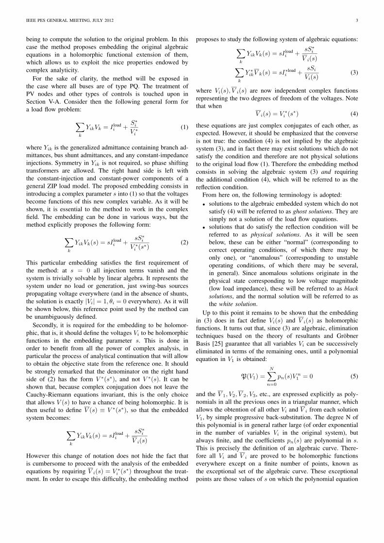
being to compute the solution to the original problem. In this

case the method proposes embedding the original algebraic

equations in a holomorphic functional extension of them,

which allows us to exploit the nice properties endowed by

complex analyticity.

For the sake of clarity, the method will be exposed in

the case where all buses are of type PQ. The treatment of

PV nodes and other types of controls is touched upon in

Section V-A. Consider then the following general form for

a load flow problem:

∑k

YikVk = I loadi +

S∗i

V ∗i

(1)

where Yik is the generalized admittance containing branch ad-

mittances, bus shunt admittances, and any constant-impedance

injections. Symmetry in Yik is not required, so phase shifting

transformers are allowed. The right hand side is left with

the constant-injection and constant-power components of a

general ZIP load model. The proposed embedding consists in

introducing a complex parameter s into (1) so that the voltages

become functions of this new complex variable. As it will be

shown, it is essential to the method to work in the complex

field. The embedding can be done in various ways, but the

method explicitly proposes the following form:

∑k

YikVk(s) = sI loadi +

sS∗i

V ∗i (s

∗)(2)

This particular embedding satisfies the first requirement of

the method: at s = 0 all injection terms vanish and the

system is trivially solvable by linear algebra. It represents the

system under no load or generation, just swing-bus sources

propagating voltage everywhere (and in the absence of shunts,

the solution is exactly |Vi| = 1, θi = 0 everywhere). As it will

be shown below, this reference point used by the method can

be unambiguously defined.

Secondly, it is required for the embedding to be holomor-

phic, that is, it should define the voltages Vi to be holomorphic

functions in the embedding parameter s. This is done in

order to benefit from all the power of complex analysis, in

particular the process of analytical continuation that will allow

to obtain the objective state from the reference one. It should

be strongly remarked that the denominator on the right hand

side of (2) has the form V ∗(s∗), and not V ∗(s). It can be

shown that, because complex conjugation does not leave the

Cauchy-Riemann equations invariant, this is the only choice

that allows V (s) to have a chance of being holomorphic. It is

then useful to define V (s) ≡ V ∗(s∗), so that the embedded

system becomes:

∑k

YikVk(s) = sI loadi +

sS∗i

V i(s)

However this change of notation does not hide the fact that

is cumbersome to proceed with the analysis of the embedded

equations by requiring V i(s) = V ∗i (s

∗) throughout the treat-

ment. In order to escape this difficulty, the embedding method

proposes to study the following system of algebraic equations:∑k

YikVk(s) = sI loadi +

sS∗i

V i(s)∑k

Y ∗ikV k(s) = sI∗load

i +sSi

Vi(s)(3)

where Vi(s), V i(s) are now independent complex functions

representing the two degrees of freedom of the voltages. Note

that when

V i(s) = V ∗i (s

∗) (4)

these equations are just complex conjugates of each other, as

expected. However, it should be emphasized that the converse

is not true: the condition (4) is not implied by the algebraic

system (3), and in fact there may exist solutions which do not

satisfy the condition and therefore are not physical solutions

to the original load flow (1). Therefore the embedding method

consists in solving the algebraic system (3) and requiring

the additional condition (4), which will be referred to as the

reflection condition.

From here on, the following terminology is adopted:

• solutions to the algebraic embedded system which do not

satisfy (4) will be referred to as ghost solutions. They are

simply not a solution of the load flow equations.

• solutions that do satisfy the reflection condition will be

referred to as physical solutions. As it will be seen

below, these can be either “normal” (corresponding to

correct operating conditions, of which there may be

only one), or “anomalous” (corresponding to unstable

operating conditions, of which there may be several,

in general). Since anomalous solutions originate in the

physical state corresponding to low voltage magnitude

(low load impedance), these will be referred to as blacksolutions, and the normal solution will be referred to as

the white solution.

Up to this point it remains to be shown that the embedding

in (3) does in fact define Vi(s) and V i(s) as holomorphic

functions. It turns out that, since (3) are algebraic, elimination

techniques based on the theory of resultants and Grobner

Basis [25] guarantee that all variables Vi can be successively

eliminated in terms of the remaining ones, until a polynomial

equation in V1 is obtained:

P(V1) =

N∑n=0

pn(s)Vn1 = 0 (5)

and the V 1, V2, V 2, V3, etc., are expressed explicitly as poly-

nomials in all the previous ones in a triangular manner, which

allows the obtention of all other Vi and V i from each solution

V1, by simple progressive back-substitution. The degree N of

this polynomial is in general rather large (of order exponential

in the number of variables Vi in the original system), but

always finite, and the coefficients pn(s) are polynomial in s.

This is precisely the definition of an algebraic curve. There-

fore all Vi and V i are proved to be holomorphic functions

everywhere except on a finite number of points, known as

the exceptional set of the algebraic curve. These exceptional

points are those values of s on which the polynomial equation

IEEE PES GENERAL MEETING, JULY 2012 4

for V1 exhibits a null derivative ∂P/∂V1, and will play an

important role on the discussion about analytic continuation

further below.

B. Power series

Obtaining and solving (5) for large networks is unfeasible in

practice. Instead, one should work with the power series of the

holomorphic functions, as is commonly done when calculating

algebraic curves. The power series provides the so-called germof the analytical function, as it allows to calculate the function

well away from the convergence radius of the series, by the

well-known mechanism of analytic continuation.

As seen above, the algebraic problem has multiple solutions.

Indeed at s = 0, multiple solutions as can be found for (3) if

one allows Vi(0) = 0 and V i(0) = 0 at one or more buses i.However, those solutions are either ghost (unphysical) or black(non-vanishing injection at s = 0, meaning a short-circuit at

the bus). On the other hand, by requiring V i(0) �= 0 and

V i(0) �= 0 for all buses i, all injection terms in (3) vanish at

s = 0 and the resulting linear system has a unique solution,

dubbed the white solution. This is the operational solution

of a power system under a no-load, no-generation scenario,

where only the swing bus is providing a voltage source. The

HELM method proposes that the operational solution to the

load flow problem is the maximal analytical continuation of

this reference solution at s = 0.

An interesting question may arise now, as to what solution

is actually realized in a real power system. Is it necessarily the

continuation of the white solution, as proposed by the method?

To answer this question satisfactorily we need to remind

ourselves that the load flow equations are just describing

the steady-state of the physical system. To be certain about

the actual state of the system we would need to integrate

the differential equations of the full dynamical model, using

some initial conditions. This would yield a unique steady

state because there is no ambiguity in the solution of those

equations. This is almost impossible to achieve in practice, but

it is certain that the steady state will be analytic in the problem

parameters, given some minimal assumptions of smoothness

for the differential equations. In the absence of this modeling,

solving the algebraic equations for the steady state actually

requires to make a proposal as to what solution is the correct

one for the physical systyem. In this sense, and invoking

the smoothness of the underlying dynamical model, it seems

most reasonable to propose the solution that is the analytical

continuation of the white solution at the reference limit s = 0.

Note however that the HELM procedure can also be applied

to the calculation of black branches, and it possibly provides

the best framework in which this can be done in a systematic

manner.

The power series for the white solution can now be calcu-

lated as follows. Assume Vi(s) =∑∞

n=0 ci[n]sn are the power

series to be calculated, and 1/Vi(s) =∑∞

n=0 di[n]sn are the

corresponding power series for the functions appearing on the

right hand side of (3). Making use of the reflection condition

V i(s) = V ∗i (s

∗), the following equation is obtained where a

formal power series appears on both sides:

∑k

Yik

∞∑n=0

ck[n]sn = sI load

i + sS∗i

∞∑n=0

d∗i [n]sn (6)

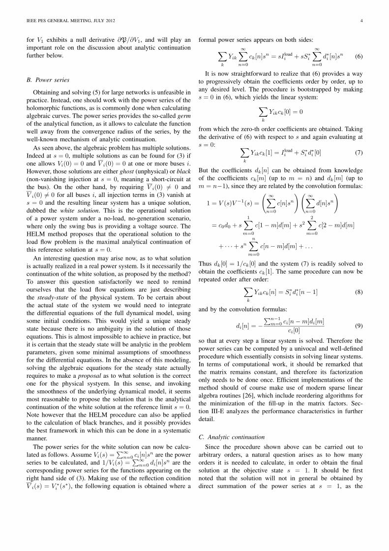
It is now straightforward to realize that (6) provides a way

to progressively obtain the coefficients order by order, up to

any desired level. The procedure is bootstrapped by making

s = 0 in (6), which yields the linear system:∑k

Yikck[0] = 0

from which the zero-th order coefficients are obtained. Taking

the derivative of (6) with respect to s and again evaluating at

s = 0: ∑k

Yikck[1] = I loadi + S∗

i d∗i [0] (7)

But the coefficients dk[n] can be obtained from knowledge

of the coefficients ck[m] (up to m = n) and dk[m] (up to

m = n−1), since they are related by the convolution formulas:

1 = V (s)V −1(s) =

( ∞∑n=0

c[n]sn

)( ∞∑n=0

d[n]sn

)

= c0d0 + s

1∑m=0

c[1−m]d[m] + s22∑

m=0

c[2−m]d[m]

+ · · ·+ snn∑

m=0

c[n−m]d[m] + . . .

Thus dk[0] = 1/ck[0] and the system (7) is readily solved to

obtain the coefficients ck[1]. The same procedure can now be

repeated order after order:∑k

Yikck[n] = S∗i d

∗i [n− 1] (8)

and by the convolution formulas:

di[n] = −∑n−1

m=0 ci[n−m]di[m]

ci[0](9)

so that at every step a linear system is solved. Therefore the

power series can be computed by a univocal and well-defined

procedure which essentially consists in solving linear systems.

In terms of computational work, it should be remarked that

the matrix remains constant, and therefore its factorization

only needs to be done once. Efficient implementations of the

method should of course make use of modern sparse linear

algebra routines [26], which include reordering algorithms for

the minimization of the fill-up in the matrix factors. Sec-

tion III-E analyzes the performance characteristics in further

detail.

C. Analytic continuation

Since the procedure shown above can be carried out to

arbitrary orders, a natural question arises as to how many

orders it is needed to calculate, in order to obtain the final

solution at the objective state s = 1. It should be first

noted that the solution will not in general be obtained by

direct summation of the power series at s = 1, as the

IEEE PES GENERAL MEETING, JULY 2012 5

radius of convergence is typically much smaller than 1. The

powerful procedure of analytic continuation is used instead

[27]. In passing, it should be stressed that the process of

analytic continuation does not have anything in common with

the concepts of numerical continuation (homotopy methods

[19]) used in continuation load flow methods. In practice the

analytical continuation is carried out by means of rational

approximants, among which Pade approximation is the method

of choice for reasons to be revealed shortly. As to the question

of the number of terms needed in the power series in order

to attain a given level of precision, practice has shown that

typically anywhere from 10 to 40 terms suffice to reach 5-digit

precision in large networks, and about 60 terms will exhaust

the limits of the computer arithmetic in double precision.

The mechanics of the method have now been completely

described, but another important issue needs to be addressed:

is the analytical continuation procedure “complete”? That is,

does it always reach the solution when it exists? Conversely,

will the procedure unambiguously signal non-existence when

the solution does not exist?. To answer these questions it

is needed to invoke some powerful results from Complex

Analysis.

As it is well-known from the theory of Algebraic Curves,

all solutions Vi(s) and V i(s) are holomorphic functions that

can be analytically continued along any path in s, as long

as this path does not contain points of the exceptional set of

the curve. This result can be alternatively stated by saying

that Algebraic Curves are analytical functions whose only

singularities are branch points, since the exceptional points

of the curve (the points in s where the zeros of (5) have

multiplicity greater than one, or equivalently, the points on the

curve where ∂P/∂V1 = 0) are in fact branch points. These

are the points where two or more branches of the curve V1(s)coalesce. The algebraic curve as a whole (all its branches)

is a complete global analytic function [28], which means

that there exist paths of analytic continuation connecting any

points between any branches. In other words, knowledge of the

power series at any (non-exceptional) point can be exploited

to calculate the solution anywhere else, on any branch, by

means of a suitable path of analytic continuation. However,

note that analytical continuation paths enclosing branch points

yield the curve on a branch different from the starting one. This

is the subject of Monodromy Theory and is a foundational

part of the theory of Riemann surfaces, which is the natural

setting in which to study multivalued complex functions (and

in particular, algebraic curves). For the purposes of the load

flow method, the aim is to perform analytic continuation of

the reference solution at s = 0 along paths that ensure single-

valuedness, in other words, remaining always within the white

branch. This is accomplished by the well-known procedure

of selecting branch cuts on the complex plane. Branch cuts

consist of lines connecting all branch points in such a way

that no analytic continuation paths can encircle isolated branch

points, in which case Monodromy Theory ensures that any

chosen path for analytical continuation is single-valued.

However, since the specific geometry of cuts is arbitrary,

some criteria need to be defined in order to choose them. At

this point, two key results are invoked:

1) Stahl’s extremal domain theorem [29]–[31]: this result

asserts that for any analytic function there exists a

unique set of cuts with the property of having minimal

logarithmic capacity [32], and such that the function

has single-valued analytic continuation in the domain

consisting of the complex plane excluding the cuts (i.e.,

the maximal domain). This provides a natural criteria for

the choice of cuts, and ensures that such choice exists

and is unique.

2) Stahl’s Pade convergence theorem [33], [34]: for any

analytic function whose singularities are finite (in fact,

it suffices for the set of singularities to have zero

logarithmic capacity), any close-to-diagonal sequence of

Pade approximants converge in capacity to said function

in the extremal domain. The poles of the diagonal and

paradiagonal Pade approximants accumulate on the set

of cuts with minimal logarithmic capacity.

Pade approximants [31] are rational approximants to power

series, and they have been used extensively as a technique

for analytic continuation because their convergence has been

known to be much better than that of power series. In

particular, the diagonal and paradiagonal Pade approximants

coincide with the continued fraction approximation to the

power series, which are also known to have good convergence

properties in general. Stahl’s results, after the seminal works of

Nuttall [35], reveal that Pade approximants are really a means

for maximal analytic continuation. Therefore these two results

confer the method very strong additional guarantees: if the

Pade approximants converge at s = 1, the result is guaranteed

to be the analytic continuation of the white branch at s = 1;

conversely, if the Pade approximants do not converge at s = 1(i.e. the point s = 1 lies on the set of cuts with minimal

logarithmic capacity) then it is guaranteed that there is no

solution (that is, the system is beyond voltage collapse).

D. The method in brief

To recapitulate, the Holomorphic Embedding Load Flow

boils down to these steps:

1) Choose a suitable complex embedding by means of

a complex parameter s. The embedding needs to be

holomorphic (uses V ∗(s∗), not V ∗(s)). At s = 0, this

embedding should be such that the system becomes

linear and trivially simple to solve (the no-load, no-

generation case). This unambiguously selects the ref-

erence solution at s = 0.

2) Calculate the power series of V (s) corresponding to the

reference solution, by means of a sequence of linear

systems that yield the coefficients progressively, order

after order. The matrix in those systems remains always

constant, so it needs to be factorized just once; and

the right hand sides can always be calculated from the

results of the previous system.

3) Compute the solution at s = 1 as the analytical continua-

tion of the power series obtained in step 2, by using Pade

Approximants. These are guaranteed to yield maximal

analytical continuation, therefore the solution is obtained

IEEE PES GENERAL MEETING, JULY 2012 6

when it exists, or a divergence is obtained when it does

not exist.

Steps 2 and 3 are typically performed in an interleaved fashion,

that is, after a new coefficient of the series is obtained, a

new Pade approximant can be computed. The procedure stops

when the desired accuracy is obtained, or when oscillation

or divergence is detected. Section IV below will illustrate the

whole procedure step by step.

E. Performance

The performance characteristics of the method are fairly

easy to analyze in the asymptotic limit, when the size N of

the network is large. Most of the work consists in factorizing

a matrix system (8), and using the result to repeatedly solve

different right-hand sides. Modern direct sparse solvers [26]

are able to factorize a matrix A into its LDLT Cholesky

decomposition with a cost of O(|L|), that is, linear in the

number of non-zero entries obtained in the factorized matrix

L. Therefore it is of utmost importance to use a fill-reducing

reordering of the matrix. Solving each system adds O(N)operations due to forward and back substitution. Computing

the right hand sides of each linear system involves computing

a simple convolution formula, reaching at most the order of

the coefficient we are solving in the series. Since in practice

there is a maximum of about 60 coefficients to solve before

one encounters the limits of double-precision accuracy, the

cost of calculation of these convolution formulas can consid-

ered to be fixed for each bus and thus contributes another

O(N). The same can be said about the computation of Pade

Approximants. The cost of computing approximants increases

approximately as the square of the number of coefficients

being used, but since this number tops off at about a maximum

of 60, the costs are still O(N) asymptotically. Moreover,

both the computation of the right-hand sides and the Pade

approximants can be trivially parallellized. Therefore for large

enough networks the costs are dominated by the factorization

of the impedance matrix. These costs are then similar to

the FDNR method, since the matrix factorization is only

performed once.

To give some practical figures, in a real-world large trans-

mission network of about 3,000 electrical nodes the HELM

algorithm solves a load flow in about 10 to 20 ms, running

on Intel Xeon 5500 CPUs, for a required precision of about

5 significant digits. The maximum orders for the Pade ap-

proximants are typically about 20, going up to a maximum of

about 60 in scenarios where the network approaches voltage

collapse.

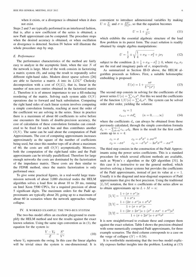
IV. A WORKED EXAMPLE: THE TWO-BUS SYSTEM

The two-bus model offers an excelent playground to exem-

plify the HELM method and test the results against the exact

known solution. Using the same sign convention as in (1), the

equation for the system is:

V − V0

Z=

S∗

V ∗ (10)

where V0 represents the swing. In this case the linear algebra

will be trivial since the system is one-dimensional. It is

convenient to introduce adimensional variables by making

U ≡ VV0

and σ ≡ ZS∗|V0|2 , so that the equation becomes

U = 1 +σ

U∗ (11)

which exhibits the essential algebraic structure of the load

flow problem in its purest form. The exact solution is readily

obtained by simple algebra manipulations:

U =1

2±√

1

4+ σR − σ2

I + jσI (12)

subject to the condition Δ ≡ 14 + σR − σ2

I ≥ 0, where σR, σI

are the real and imaginary parts of σ, respectively.

As summarized in Section III-D above, the HELM al-

gorithm proceeds as follows. First, a suitable holomorphic

embedding is proposed:

U(s) = 1 +sσ

U∗(s∗)(13)

The second step consists in solving for the coefficients of the

power series U(s) =∑

cnsn. For this we need the coefficients

of the function 1/U(s) =∑

dnsn. The system can be solved

order after order, yielding the solution:

c0 = 1

cn+1 = σd∗n (n = 0, . . . ,∞) (14)

where the coefficients dn can always be obtained from those

previously calculated, through the simple convolution formula

dn = −∑n−1k=0 cn−kdk. Here is the result for the first coeffi-

cients up to n = 4:

c1 = σc2 = −σσ∗

c3 = σ2σ∗ + σσ∗2

c4 = −σ3σ∗ − 3σ2σ∗2 − σσ∗3

The third step consists in the construction of the Pade Approx-

imants using the power series coefficients. This is a standard

procedure for which several efficient methods are available,

such as Wynn’s ε algorithm or the QD algorithm [31]. In

this case it is instructive to use the general method, which

involves solving a linear systems but provides the coefficients

of the Pade approximants, instead of just its value at s = 1.

Usually it is the diagonal and near-diagonal sequences of Pade

approximants that give the best precision. Using the traditional

[L/M ] notation, the first n coefficients of the series allow us

to obtain approximants up to L+M = n:

[1/1] =1 + (σ + σ∗)s

1 + σ∗s

[2/1] =1 + (2σ + σ∗)s+ σ2s2

1 + (σ + σ∗)s

[2/2] =1 + (2σ + 2σ∗)s+ (σ2 + σσ∗ + σ∗2)s2

1 + (σ + 2σ∗)s+ σ∗2s2

It is now straightforward to evaluate these and compare them

against the exact solution. Table I shows the precision obtained

with some numerically computed Pade approximants, for three

example scenarios. The third column corresponds to a case on

the verge of collapse (|V | = 0.58).

It is worthwhile mentioning that the two-bus model explic-

itly exposes further insights into the problem. Looking at (13)

IEEE PES GENERAL MEETING, JULY 2012 7

TABLE IEXAMPLES OF RELATIVE PRECISION OF PADE APPROXIMANTS VS. ORDER

Pade order σ = −0.07− j0.08 −0.14− j0.15 −0.2− j0.22(|V | = 0.92) (|V | = 0.81) (|V | = 0.58)

[2/2] 1.795e-03 2.30e-02 2.74e-01[5/5] 7.02e-09 2.10e-05 5.85e-02[10/10] 0 1.89e-10 1.16e-02[15/15] 0 1.55e-15 2.86e-03[20/20] 0 0 7.38e-04

and its complex comjugate, it is realized that the equations are

telling us explicitely what the solution is, in continued fractionform. Just subsitute the denominators iteratively:

U(s) = 1 +σs

1 +σ∗s

1 +σs

1 +σ∗s

1 + · · ·

(15)

This is another representation of the function, but continued

fractions have in general a much larger convergence radius

and faster convergence compared to power series. In fact, it

is well known that the convergents (i.e. truncations) of this

continued fraction coincide with the diagonal and paradiagonal

Pade approximants [31]. This may be verified against the

approximants computed above in (15).

The general N -bus case does not easily lend itself into

the elegant continued fraction approach, since there are linear

systems involved. However, given the equivalence between

Pade approximants and continued fractions, the analysis of

the two-bus model is quite relevant, as the essential algebraic

structure of the problem is already there.

V. FINAL REMARKS

A. Controls

Thus far only the pure PQ case has been considered. Real

power systems have all sorts of automated controls imposing

additional constraints on the solution of (1), the most pervasive

being the PV controls for generator buses. These and other

controls such as transformer ULTCs, FACTS, o HVDC links

are easily accommodated under the HELM methodology.

The explicit procedure for each type of constraint, although

straightforward, is lengthy and will be the subject of a follow

on paper [36]. Here it is pointed out that the only requirement

is that the constraints can be expressed as algebraic equalities,

which is true in all the aforementioned cases. Since no

approximations are needed, the solutions benefit from all the

mathematical guarantees that have been shown in this paper.

This is in contrast to iterative methods, where controls are

introduced as adjustments at each iteration. Such adjustments

do not lend themselves to rigorous analysis and their effects

on the solutions have to be studied empirically [37], [38].

B. Significance of HELM

Arguably the single most important impact of the HELM

algorithm is the enabling of reliable, real-time, intelligent

applications. The HELM method was actually born out of the

need for a fully reliable load flow in the context of some

AI-based applications that depend critically on the ability

to perform exploratory load flow studies, with absolutely

no margin for failure. The most prominent examples are

two decision-support tools, a Limits Violation Solver and a

Restoration Plan Builder. These tools are fully model-based

thanks to a technique well-known in the AI community: guided

exploration in the state-space of the electrical system, using

the A∗ algorithm. The state-space consists of all possible

electrical (steady) states that the network can achieve, and the

available SCADA actions provide transitions between them.

The algorithm needs sophisticated heuristics to guide the

search efficiently, but the load flow method needs to be 100%

reliable, as it is used at each and every step of the exploration.

Our experience has shown that these kind of tools would be

impossible to build on top of iterative load flow methods. Of

course, other real-time tools such as Contingency Analysis or

PV/QV Curves also benefit from increased reliability.

Another promising yet untapped potential of the method

lies in the new insights it brings into the analysis of the load

flow problem. The treatment in terms algebraic curves could

prove quite powerful. For instance, it provides a coherent

framework for the characterization and computation of all

the multiple solutions to the original problem (white, black,

ghost solutions). Given the vast amounts of results in the

field of algebraic curves in Complex Analysis, it is reasonable

to think that this is just scratching the surface of what is

potentially possible. The theory of approximants (rational or

other) is another source for insights and practical results.

As it has been shown, the zeros and poles of the rational

approximants tend to accumulate on the (minimal) branch cuts

of the functions V (s). Therefore their values, or even their

patterns of appearance as the approximant order increases, may

be used as new indicators, such as the proximity to voltage

colapse. One may think of all this as a sort of a new language

for the analysis of an old problem.

VI. CONCLUSIONS

This paper has presented a novel load flow method that rad-

ically breaks away from the established iterative methods. Its

most salient features are that it is non-iterative, deterministic,

and non-ambiguous: it guarantees, backed by mathematical

proof, obtaining the right solution to the multivalued load

flow problem, and otherwise signals unambiguously the non-

existence of solution when the system is beyond voltage

collapse. The method is based on a holomorphic embedding

procedure that extends the voltage variables into analytic

functions in the complex plane. This provides a framework to

study and obtain the solutions using the full power of complex

analysis. The method provides a procedure for constructing the

complex power series at a well-defined reference point, where

it is trivial to identify the correct branch of the multivalued

problem, and then uses analytical continuation by means of

algebraic approximants to reach the objective. It can be proven

that the continuation is maximal in logarithmic capacity,

thus propagating the chosen branch to the maximal possible

IEEE PES GENERAL MEETING, JULY 2012 8

domain on the complex plane. If the objective point is not

in this domain, the initial correct branch does not have an

analytical continuation there and the problem has no solution.

Therefore, by construction, the process is totally deterministic

thus ensuring that if there is a solution the method will find it

and, conversely, if there is no solution (voltage collapse) the

method will unequivocally signal such condition as well.

Although advanced results from geometric function theory

are used to prove the method properties, the numerical im-

plementation is straightforward and has performance charac-

teristics that make it competitive and even superior to fast-

decoupled algorithms, thus making it a good general-purpose

load flow method for power systems of any size. The method

has been implemented in industrial-strength EMS applications

now operating at several large transmission operators, and has

been granted two US Patents [39]. Experience has proven the

foremost practical impact of the method, namely the enabling

of reliable real-time applications.

ACKNOWLEDGMENT

The author would like to thank J. A. Marques and V. Gaitan

for their numerical implementations and extensive testing of

the HELM algorithms since its inception, and J. L. Marın

for his help in the preparation of this manuscript. The author

also thanks the reviewers of the manuscript, whose comments

helped improve the clarity of the paper.

REFERENCES

[1] A. Gomez-Exposito and F. L. Alvarado, “Load flow,” in Electric EnergySystems: Analysis and Operation, A. Gomez-Exposito, A. J. Conejo, andC. Canizares, Eds. CRC Press, 2009, pp. 95–126.

[2] J. B. Ward and H. W. Hale, “Digital computer solution of power-flowproblems,” Power Apparatus and Systems, Part III. Transactions of theAmerican Institute of Electrical Engineers, vol. 75, no. 3, pp. 398–404,jan. 1956.

[3] W. Tinney and C. Hart, “Power flow solution by newton’s method,”IEEE Trans. Power App. Syst., vol. PAS-86, no. 11, pp. 1449–1460,nov. 1967.

[4] W. Tinney and J. Walker, “Direct solutions of sparse network equationsby optimally ordered triangular factorization,” Proc. IEEE, vol. 55,no. 11, pp. 1801–1809, nov. 1967.

[5] S. Despotovic, B. Babic, and V. Mastilovic, “A rapid and reliable methodfor solving load flow problems,” IEEE Trans. Power App. Syst., vol.PAS-90, no. 1, pp. 123–130, jan. 1971.

[6] B. Stott, “Decoupled newton load flow,” IEEE Trans. Power App. Syst.,vol. PAS-91, no. 5, pp. 1955–1959, sept. 1972.

[7] B. Stott and O. Alsac, “Fast decoupled load flow,” IEEE Trans. PowerApp. Syst., vol. PAS-93, no. 3, pp. 859–869, may 1974.

[8] R. van Amerongen, “A general-purpose version of the fast decoupledload flow,” IEEE Trans. Power Syst., vol. 4, no. 2, pp. 760–770, may1989.

[9] G. Leonidopoulos, “Approximate linear decoupled solution as the initialvalue of power system load flow,” Electric Power Systems Research,vol. 32, no. 3, pp. 161–163, 1995.

[10] R. Klump and T. Overbye, “Techniques for improving power flowconvergence,” in Power Engineering Society Summer Meeting, 2000.IEEE, vol. 1, 2000, pp. 598–603.

[11] F. Wu, “Theoretical study of the convergence of the fast decoupled loadflow,” IEEE Trans. Power App. Syst., vol. 96, no. 1, pp. 268–275, jan.1977.

[12] J. Hubbard, D. Schleicher, and S. Sutherland, “How to find all roots ofcomplex polynomials by newton’s method,” Inventiones Mathematicae,vol. 146, pp. 1–33, 2001.

[13] R. Klump and T. Overbye, “A new method for finding low-voltage powerflow solutions,” in Power Engineering Society Summer Meeting, 2000.IEEE, vol. 1, 2000, pp. 593–597.

[14] J. Thorp and S. Naqavi, “Load-flow fractals draw clues to erraticbehaviour,” IEEE Comput. Appl. Power, vol. 10, no. 1, pp. 59–62, jan1997.

[15] Grupo AIA, “Problems with iterative load flow,” http://www.elequant.com/products/agora/demo/iterativeloadflow, 2002–11.

[16] I. Dobson, “Observations on the geometry of saddle node bifurcationand voltage collapse in electrical power systems,” IEEE Trans. CircuitsSyst. I, vol. 39, no. 3, pp. 240–243, mar 1992.

[17] C. Canizares, “On bifurcations, voltage collapse and load modeling,”IEEE Trans. Power Syst., vol. 10, no. 1, pp. 512–522, feb 1995.

[18] V. Ajjarapu and C. Christy, “The continuation power flow: a tool forsteady state voltage stability analysis,” IEEE Trans. Power Syst., vol. 7,no. 1, pp. 416–423, feb 1992.

[19] E. Allgower and K. Georg, Introduction to numerical continuationmethods, ser. Classics in applied mathematics. SIAM, 2003.

[20] A. Montes, “Algebraic solution of the load-flow problem for a 4-nodeselectrical network,” Mathematics and Computers in Simulation, vol. 45,no. 1-2, pp. 163–174, 1998.

[21] J. Ning, W. Gao, G. Radman, and J. Liu, “The application of thegroebner basis technique in power flow study,” in North American PowerSymposium (NAPS), 2009, oct. 2009, pp. 1–7.

[22] W. Xu, Y. Liu, J. Salmon, T. Le, and G. Chang, “Series load flow:a novel noniterative load flow method,” Generation, Transmission andDistribution, IEE Proceedings, vol. 145, no. 3, pp. 251–256, may 1998.

[23] A. Zambroni De Souza, C. Rosa, B. Lima Lopes, R. Leme, andO. Carpinteiro, “Non-iterative load-flow method as a tool for voltagestability studies,” Generation, Transmission Distribution, IET, vol. 1,no. 3, pp. 499–505, may 2007.

[24] P. Sauer, “Explicit load flow series and functions,” IEEE Trans. PowerApp. Syst., vol. PAS-100, no. 8, pp. 3754–3763, aug. 1981.

[25] B. Sturmfels, Solving systems of polynomial equations, ser. Regionalconference series in mathematics. AMS, 2002.

[26] T. Davis, Direct methods for sparse linear systems, ser. Fundamentalsof algorithms. SIAM, 2006.

[27] T. Gamelin, Complex analysis. Springer, 2001.[28] L. Ahlfors, Complex analysis: an introduction to the theory of analytic

functions of one complex variable. McGraw-Hill, 1979.[29] H. Stahl, “Extremal domains associated with an analytic function I, II,”

Complex Variables, Theory and Application: An International Journal,vol. 4, no. 4, pp. 311–324, 325–338, 1985.

[30] ——, “The structure of extremal domains associated with an analyticfunction,” Complex Variables, Theory and Application: An InternationalJournal, vol. 4, no. 4, pp. 339–354, 1985.

[31] G. Baker and P. Graves-Morris, Pade approximants, ser. Encyclopediaof mathematics and its applications. Cambridge University Press, 1996.

[32] R. Rumely, Capacity theory on algebraic curves, ser. Lecture notes inmathematics. Springer-Verlag, 1989.

[33] H. Stahl, “On the convergence of generalized Pade approximants,”Constructive Approximation, vol. 5, pp. 221–240, 1989.

[34] ——, “The convergence of Pade approximants to functions with branchpoints,” Journal of Approximation Theory, vol. 91, no. 2, pp. 139–204,1997.

[35] J. Nuttall, “On convergence of Pade approximants to functions withbranch poits,” in Pade and Rational Approximation, E. B. Saff and R. S.Varga, Eds. Academic Press, New York, 1977, pp. 101–109.

[36] A. Trias, “Holomorphic embedding load flow: Controls,” 2012, preprint.[37] S.-K. Chang and V. Brandwajn, “Solving the adjustment interactions in

fast decoupled load flow,” IEEE Trans. Power Syst., vol. 6, no. 2, pp.801–805, may 1991.

[38] J. Vlachogiannis, “Control adjustments in fast decoupled load flow,”Electric Power Systems Research, vol. 31, no. 3, pp. 185–194, 1994.

[39] A. Trias, “System and method for monitoring and managing electricalpower transmission and distribution networks,” US Patents 7 519 506and 7 979 239, 2009–2011.

Antonio Trias received a PhD degree in Physics from the University ofBarcelona in 1974. From 1974 to 1976 he was a visiting postdoctoral researchfellow at the Lawrence Berkeley Laboratory of the University of California.He is a founding member of Aplicaciones en Informatica Avanzada S.A.,where he currently is R&D Vice President and CTO. He has worked in theload flow problem and other algorithms of interest for power systems for overtwenty years.