Embed Size (px)
Citation preview
IECM Technical Documentation:
Chemical Looping Combustion
for Pre-combustion CO2 Capture
September 2012
Disclaimer
This report was prepared as an account of work sponsored by an agency of the United
States Government. Neither the United States Government nor any agency thereof,
nor any of their employees, makes any warranty, express or implied, or assumes any
legal liability or responsibility for the accuracy, completeness, or usefulness of any
information, apparatus, product, or process disclosed, or represents that its use would
not infringe privately owned rights. Reference therein to any specific commercial
product, process, or service by trade name, trademark, manufacturer, or otherwise
does not necessarily constitute or imply its endorsement, recommendation, or
favoring by the United States Government or any agency thereof. The views and
opinions of authors expressed therein do not necessarily state or reflect those of the
United States Government or any agency thereof.
IECM Technical Documentation:
Chemical Looping Combustion for Pre-combustion CO2 Capture
RES Activity No. 0004000.2.672.241.003:
The Role of Simulation and Modeling in Accelerating CO2 Capture Technology
Prepared for:
National Energy Technology Laboratory
Department of Energy
Pittsburgh, PA 15236
www.netl.doe.gov
Prepared by:
Hari C. Mantripragada
Edward S. Rubin
Carnegie Mellon University
Pittsburgh, PA 15213
www.iecm-online.com
September 2012

Integrated Environmental Control Model - Technical Documentation Table of Contents v
Table of Contents
Chemical Looping Combustion 1
Objectives of this Report ........................................................................................................... 1 Introduction ............................................................................................................................... 2
Oxygen Carriers .......................................................................................................... 3 Reactor Design ............................................................................................................ 4 CLC Applications ........................................................................................................ 5
Thermodynamic Analysis of CLC Reactions .......................................................................... 10 Equilibrium Constant Solution Method ..................................................................... 10 Adiabatic Temperature .............................................................................................. 12 Air Reactor Calculations ........................................................................................... 13 Fuel Reactor Analysis................................................................................................ 19 Methods for Calculating Solids Inventory ................................................................. 30 Reactor Design .......................................................................................................... 32
IGCC power plant using CLC ................................................................................................. 34 Gas turbine and compressor calculations .................................................................. 34 CO2 Purification Unit ................................................................................................ 35 Calculation procedure ................................................................................................ 38
Case Studies ............................................................................................................................. 40 Base Case .................................................................................................................. 40 Results ....................................................................................................................... 41
Conclusion ............................................................................................................................... 48 References ............................................................................................................................... 48
Integrated Environmental Control Model - Technical Documentation List of Figures vi
List of Figures
Figure 1. Chemical looping combustion process: Oxygen carrier is oxidized in the air reactor and reduced in the fuel
reactor. .......................................................................................................................................................................... 2
Figure 2. Typical process flow diagram of CLC process with interconnected fluidized beds (1) high velocity riser air
reactor, (2) cyclone for particle separation and (3) fuel reactor (Fang et al, 2009) ...................................................... 5
Figure 3. Example of application of CLC to power generation – a simple cycle power plant where hot exhaust from air
(oxidation) and fuel (reduction) reactors are expanded in air and CO2 turbines, respectively (Brandvoll and Bolland,
2004). ............................................................................................................................................................................ 6
Figure 4. Example of a CLC combined cycle power plant. Steam is produced using the hot exhaust from air and CO2
turbines in a heat recovery steam generator (HRSG) (Naqvi and Bolland, 2007). ....................................................... 7
Figure 5. Conceptual design of combined gasification and combustion of solid fuels using chemical looping (Rizeq et al,
2003). ............................................................................................................................................................................ 8
Figure 6. ALSTOM's Ca-based CLC process (Andrus et al, 2009). ..................................................................................... 8
Figure 7. Different applications of ALSTOM's chemical-looping concept using solid fuels (Andrus, 2009) ..................... 9
Figure 8. Chemical looping with oxygen-uncoupling (Mattisson et al, 2009). .................................................................... 9
Figure 9. Schematic of chemical looping combustion ........................................................................................................ 14
Figure 10. Variation of equilibrium constant for the oxidation reaction Ni + 0.5O2 <=> NiO, with temperature ............. 14
Figure 11. Inlet and outlet flows of the air reactor.............................................................................................................. 14
Figure 12. Variation of heat of reaction of Ni + 0.5O2 NiO, with temperature ............................................................. 16
Figure 13. Variation of adiabatic reaction temperature of AR as a function of inlet OC temperature at different inlet air
temperatures. Pure NiO is assumed. x=0, z=0. ........................................................................................................... 18
Figure 14. Variation of adiabatic reaction temperature of AR as a function of inlet air temperature and inlet OC
temperatures. Pure NiO is assumed. x=0, z=0. ........................................................................................................... 18
Figure 15. Variation of adiabatic temperature of AR as a function of inlet air temperature and inlet OC temperature. 40%
NiO in the OC, x=0, z=0............................................................................................................................................. 18
Figure 16. Variation of adiabatic temperature in AR as a function of excess air ratio (x) and excess NiO ratio (z) at fixed
inlet temperature of 400oC and inlet OC temperature of 900
oC ................................................................................. 19
Figure 17. Equilibrium constants for reactions between CO and NiO and H2 and NiO as a function of temperature ....... 22
Figure 18. Variation of specific heat (Cp) of different components with temperature ....................................................... 27
Figure 19. Variation of equilibrium constant expressions with temperature ...................................................................... 27
Figure 20. Variation of equilibrium constant expressions with temperature ...................................................................... 27
Figure 21. Adiabatic FR temperature as a function of inlet fuel temperature and inlet OC temperature. z=0, pure NiO as
OC .............................................................................................................................................................................. 28
Integrated Environmental Control Model - Technical Documentation List of Figures vii
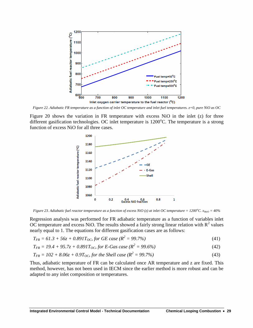
Figure 22. Adiabatic FR temperature as a function of inlet OC temperature and inlet fuel temperatures. z=0, pure NiO as
OC .............................................................................................................................................................................. 29
Figure 23. Adiabatic fuel reactor temperature as a function of excess NiO (z) at inlet OC temperature = 1200oC. xMeO =
40% ............................................................................................................................................................................. 29
Figure 24. Regression lines for solids inventory for different fuels at Xox values very close to 1. Data from Abad et al
(2007) and Mattison et al (2007) were used in estimating these. ................................................................................ 31
Figure 25. Schematic of CLC process applied to IGCC ..................................................................................................... 34
Figure 26. Flow diagram of CO2 purification unit (CPU) .................................................................................................. 35
Figure 27. Figure showing the energy requirement per tonne of CO2 cpatured as a function of the amount of inert
material (expressed in terms of N2) present in the feed gas. This figure is adopted from Aspelund and Jordal (2007).
.................................................................................................................................................................................... 37
Figure 28. Diagram showing IECM screen with performance results of a CLC reactor system ........................................ 42
Figure 29. Diagram showing IECM screen with performance results of a CLC gas turbine power block ......................... 42
Figure 30. Diagram showing IECM screen with performance results of a CLC steam cycle power block ........................ 42
Figure 31. Fuel reactor temperature as a function of air reactor temperature for excess NiO ratio at FR outlet = 0.3 ....... 43
Figure 32. Required excess air as a function of air reactor temperature for excess NiO ratio at FR outlet = 0.3 ............... 43
Figure 33. Net plant power output as a function of air reactor temperature for excess NiO ratio at FR outlet = 0.3 ......... 44
Figure 34. Net plant efficiency as a function of air reactor temperature for excess NiO ratio at FR outlet = 0.3 .............. 44
Figure 35.FR temperature as function of excess NiO ratio at FR outlet and AR temperature ............................................ 45
Figure 36. Required excess air ratio as function of excess NiO ratio at FR outlet and AR temperature ............................ 45
Figure 37. Net plant power output as function of excess NiO ratio at FR outlet and AR temperature ............................... 45
Figure 38. Net plant efficiency as function of excess NiO ratio at FR outlet and AR temperature .................................... 46
Figure 39. Mass flow rate of oxygen carrier as a function of excess NiO ratio at FR outlet and air reactor temperature .. 46
Figure 40. Total capital requirement for the CLC system as a function of air reactor temperature .................................... 47
Figure 41. Overall plant capital cost as a function of air reactor temperature .................................................................... 47
Figure 42.Total capital requirement of the CLC system as a function of excess NiO ratio at FR outlet and air reactor
temperature ................................................................................................................................................................. 47
Integrated Environmental Control Model - Technical Documentation List of Tables viii
List of Tables
Table 1. Thermodynamic properties of different species relevant for CLC applications ................................................... 13
Table 2. Equilibrium constants of different FR reactions at different temperatures ........................................................... 21
Table 3. Mass balance equations for FR ............................................................................................................................. 24
Table 4. Specific heats and other coefficients of different components used for calculation of FR adiabatic temperature 26
Table 5. Solids inventory for different fuels as a function of conversion variation. Estimated from Abad et al (2007) and
Mattisson et al (2007). ................................................................................................................................................ 30
Table 6. Design parameters of GE 7EA turbine ................................................................................................................. 34
Table 7. Input assumptions in IECM for base case ............................................................................................................ 40
Table 8.CLC Capital cost assumptions for base case ......................................................................................................... 41
Table 9. Syngas composition before and after the fuel reactor ........................................................................................... 41
Integrated Environmental Control Model - Technical Documentation Acknowledgements ix
Acknowledgements
This work is supported by the U.S. Department of Energy under Activity No.
0004000.2.672.241.003 from the National Energy Technology Laboratory (DOE/NETL). Any
opinions, findings, and conclusions or recommendations expressed in this material are those of the
authors and do not reflect the views of any agency.
We thank Haibo Zhai (Project Manager for IECM) and Karen Kietzke (Research Programmer for
IECM) of Carnegie Mellon University for their months of tireless efforts in converting the analytical
models into the user-friendly interface of IECM.
Integrated Environmental Control Model - Technical Documentation Chemical Looping Combustion 1
Chemical Looping Combustion
Objectives of this Report This report deals with the use of chemical looping combustion (CLC) technology for pre-
combustion CO2 capture from an integrated gasification combined cycle (IGCC) power plant. A
brief literature review of the CLC process is provided along with the description of the process.
In the latter part of the report, the thermodynamic principles of CLC process are explained and a
thermodynamic performance model, including reactor design, is developed which is
implemented in to the Integrated Environmental Control Model (IECM). Cost models were
developed based on data from open literature to estimate the cost of CLC system and its effect on
the overall plant costs. The models are illustrated with case studies towards the end.
Integrated Environmental Control Model - Technical Documentation Chemical Looping Combustion 2
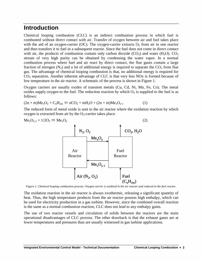
Introduction Chemical looping combustion (CLC) is an indirect combustion process in which fuel is
combusted without direct contact with air. Transfer of oxygen between air and fuel takes place
with the aid of an oxygen-carrier (OC). The oxygen-carrier extracts O2 from air in one reactor
and then transfers it to fuel in a subsequent reactor. Since the fuel does not come in direct contact
with air, the products of combustion contain only carbon dioxide (CO2) and water (H2O). CO2
stream of very high purity can be obtained by condensing the water vapor. In a normal
combustion process where fuel and air react by direct contact, the flue gases contain a large
fraction of nitrogen (N2) and a lot of additional energy is required to separate the CO2 from flue
gas. The advantage of chemical looping combustion is that, no additional energy is required for
CO2 separation. Another inherent advantage of CLC is that very less NOx is formed because of
low temperature in the air reactor. A schematic of the process is shown in Figure 1.
Oxygen carriers are usually oxides of transient metals (Cu, Cd, Ni, Mn, Fe, Co). The metal
oxides supply oxygen to the fuel. The reduction reaction by which O2 is supplied to the fuel is as
follows:
(2n + m)MexOy + CnH2m nCO2 + mH2O + (2n + m)MexOy-1 (1)
The reduced form of metal oxide is sent to the air reactor where the oxidation reaction by which
oxygen is extracted from air by the O2-carrier takes place:
MexOy-1 + 1/2O2 MexOy (2)
Figure 1. Chemical looping combustion process: Oxygen carrier is oxidized in the air reactor and reduced in the fuel reactor.
The oxidation reaction in the air reactor is always exothermic, releasing a significant quantity of
heat. Thus, the high temperature products from the air reactor possess high enthalpy, which can
be used for electricity production in a gas turbine. However, since the combined overall reaction
is the same as a normal combustion reaction, CLC does not lead to any enthalpy gains.
The use of two reactor vessels and circulation of solids between the reactors are the main
operational disadvantages of CLC process. The other drawback is that the exhaust gases are at
lower temperatures and pressures than are usually witnessed in gas turbine applications.
Air
Reactor
Air (N2, O2)
N2, O2
Fuel
Reactor
Fuel
(CnH2m)
CO2, H2O
MexOy
MexOy-1
Air
Reactor
Air (N2, O2)
N2, O2
Fuel
Reactor
Fuel
(CnH2m)
CO2, H2O
MexOy
MexOy-1
Integrated Environmental Control Model - Technical Documentation Chemical Looping Combustion 3
Oxygen Carriers
The oxygen carrier is the most important component of a CLC system. The role of an OC is to
efficiently transfer O2 between air and fuel. Hence, it must have high reactivity with both air and
fuel. Since CLC is a cyclic process, the OC should also possess mechanical strength to sustain
for a long time. Apart from that, in order to be used in a fluidized bed reactor, OC should also
possess good fluidizing properties. So, the three main requirements of an OC are:
Reactivity – should have high reactivity with both air and fuel
Durability – should be able to sustain long cyclic oxidation and reduction processes without
fragmentation or attrition
Fluidizability – should be fluidizable and stable in cyclic processes
Besides these, the OC must also be abundantly available, environmentally benign and cost less.
Oxides of transition metals such as Cu, Cd, Ni, Mn, Fe and Co are the preferred oxygen carriers
for CLC.
Though the pure metal oxides have reactive properties, they are often alloyed with support
materials to enhance the properties. Having a porous support increases the surface area for
reaction, acts as a binder to improve the mechanical strength and improves resistance to attrition.
A few typical metal oxides and porous support materials are discussed here.
Ni-based OCs
Ni-based OCs have all the desirable characteristics for CLC mainly because they can operate at
high temperatures (> 900oC) and have good methane conversion rates. The disadvantage is that
Ni is conducive to the formation of CO and H2.
It is widely observed that NiO supported over an inert material has higher reactivity and
mechanical strength than pure NiO. Examples of support materials include Yttria-stabilized-
Zirconia (YSZ), Al2O3, NiAl2O4, MgAl2O4, oxides of Si, Ti, Zr and so on. Of these, NiO coated
with NiAl2O4 has the highest potential to be an OC for a CLC process for applications using
natural gas or syngas as the fuel because of its high reactivity in oxidation and reduction, high
selectivity of CH4 to CO2 and H2O and high mechanical strength and durability over a wide
temperature range. It is relatively inexpensive too.
Cu-based OCs
CuO/Cu has the advantage of having the highest oxygen carrying capacity among the metal
oxides. High O2-carrying capacity leads to low solids flow rate. Its reduction reaction with fuel is
also exothermic which means that no additional heat is required for the reaction to take place.
Thermodynamically also, CuO/Cu is favored for complete conversion in the reduction reaction.
Besides, Cu is one of the cheapest metals. However, reactivity of this metal oxide reduces after a
few cycles and it cannot operate at high temperatures.
In order to improve the reactivity of CuO/Cu systems, Al2O3 and SiO2 have been tried as binder
materials. Though reactivity can be improved, high-temperature operation still is an area of
concern.
Fe-based OCs
Integrated Environmental Control Model - Technical Documentation Chemical Looping Combustion 4
Iron oxides are abundantly available in nature in various forms – magnetite (Fe3O4), hematite
(Fe2O3) and wustite (FeO). Hence, iron based oxygen carriers have high environmental
compatibility. Because of their abundance, their prices are lower than the oxides of Cu or Ni. Of
these, Fe2O3/Fe3O4 combination has the fastest reduction rate, and hence is more favored than
Fe3O4/FeO or FeO/Fe combinations.
Though pure Fe2O3 has excellent chemical stability at lower temperatures (<800oC), it is prone to
agglomeration at higher temperatures. Addition of supports such as Al2O3 and MgAl2O4
improves reactivity and mechanical strength but there is scope for further improvement in high-
temperature operation.
However, Fe2O3 can be used as on oxygen carrier for CLC of solid fuels like coal because it
enhances gasification reactions, which need to occur before the actual combustion begins.
Mn-based
Though it is a promising metal oxide, it has not been widely tested so far. The disadvantage of
manganese oxides is their incompatibility with common support materials like Al2O3 and SiO2.
But Mn2O3 with ZrO2 as the support material has very high reactivity and mechanical strength.
Its feasibility as an oxygen carrier will be known only after wide-scale testing.
Based on the above brief description, Ni-based oxygen carriers are likely to be favored for
gaseous fuel CLC.
Mixed metal oxides
Mixed metal oxides, which are a combination of oxides of two or more metals, are novel
materials which aim to avoid the disadvantages and combine the advantages of individual metal
oxides. For example, though CuO cannot operate at high temperatures and NiO leads to the
formation of CO and H2 in the products, the combination of CuO and NiO can be operated at
high temperatures without CO-formation. Though mixed metal oxides have not been widely
tested, they do have potential to become efficient oxygen carriers for CLC.
Others
Besides the metal oxides discussed above, other oxygen carriers have also been tried for their
applicability to CLC.
Perovskites are materials in which metal oxides are combined in a non-stoichiometric ratio,
thereby introducing structural and electronic defects that can be used to enhance reactivity.
Though some of them (eg. La0.8Sr0.2Co0.2Fe0.2O3-δ) have been tested, a lot of improvement is still
needed for them to be used as oxygen carriers for CLC.
CaSO4 has also been tried as an oxygen carrier. Though it exhibits good reactivity and stability,
the formation of SO2 at high temperatures is a definite disadvantage.
Reactor Design
The reactors in which CLC reactions take place should ensure good contact between reactants
(fuel or air) and oxygen carriers so that maximum conversion is achieved. Also, since there are
two reactors – air reactor and fuel reactor – solid flow occurs between the two reactors
continuously. There should also be minimum loss of oxygen carrier in the circulation loop.
Based on these requirements, interconnected fluidized bed reactors seem to be the ideal design
Integrated Environmental Control Model - Technical Documentation Chemical Looping Combustion 5
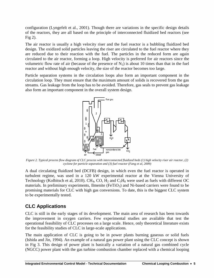
configuration (Lyngefelt et al., 2001). Though there are variations in the specific design details
of the reactors, they are all based on the principle of interconnected fluidized bed reactors (see
Fig 2).
The air reactor is usually a high velocity riser and the fuel reactor is a bubbling fluidized bed
design. The oxidized solid particles leaving the riser are circulated to the fuel reactor where they
are reduced due to their reaction with the fuel. The particles in the reduced form are again
circulated to the air reactor, forming a loop. High velocity is preferred for air reactors since the
volumetric flow rate of air (because of the presence of N2) is about 10 times than that in the fuel
reactor and without high enough velocity, the size of the reactor becomes too large.
Particle separation systems in the circulation loops also form an important component in the
circulation loop. They must ensure that the maximum amount of solids is recovered from the gas
streams. Gas leakage from the loop has to be avoided. Therefore, gas seals to prevent gas leakage
also form an important component in the overall system design.
Figure 2. Typical process flow diagram of CLC process with interconnected fluidized beds (1) high velocity riser air reactor, (2)
cyclone for particle separation and (3) fuel reactor (Fang et al, 2009)
A dual circulating fluidized bed (DCFB) design, in which even the fuel reactor is operated in
turbulent regime, was used in a 120 kW experimental reactor at the Vienna University of
Technology (Kolbitsch et al, 2010). CH4, CO, H2 and C3H8 were used as fuels with different OC
materials. In preliminary experiments, Ilmenite (FeTiO3) and Ni-based carriers were found to be
promising materials for CLC with high gas conversions. To date, this is the biggest CLC system
to be experimentally tested.
CLC Applications
CLC is still in the early stages of its development. The main area of research has been towards
the improvement in oxygen carriers. Few experimental studies are available that test the
operational feasibility of CLC processes on a large scale. Hence, only theoretical literature exists
for the feasibility studies of CLC in large-scale applications.
The main application of CLC is going to be in power plants burning gaseous or solid fuels
(Ishida and Jin, 1994). An example of a natural gas power plant using the CLC concept is shown
in Fig 3. This design of power plant is basically a variation of a natural gas combined cycle
(NGCC) power plant with the gas turbine combustion chamber replaced with a chemical looping
Integrated Environmental Control Model - Technical Documentation Chemical Looping Combustion 6
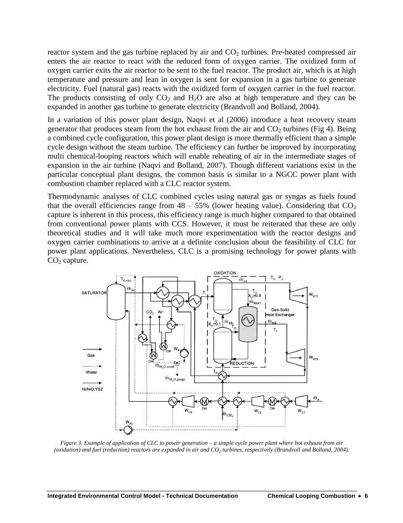
reactor system and the gas turbine replaced by air and CO2 turbines. Pre-heated compressed air
enters the air reactor to react with the reduced form of oxygen carrier. The oxidized form of
oxygen carrier exits the air reactor to be sent to the fuel reactor. The product air, which is at high
temperature and pressure and lean in oxygen is sent for expansion in a gas turbine to generate
electricity. Fuel (natural gas) reacts with the oxidized form of oxygen carrier in the fuel reactor.
The products consisting of only CO2 and H2O are also at high temperature and they can be
expanded in another gas turbine to generate electricity (Brandvoll and Bolland, 2004).
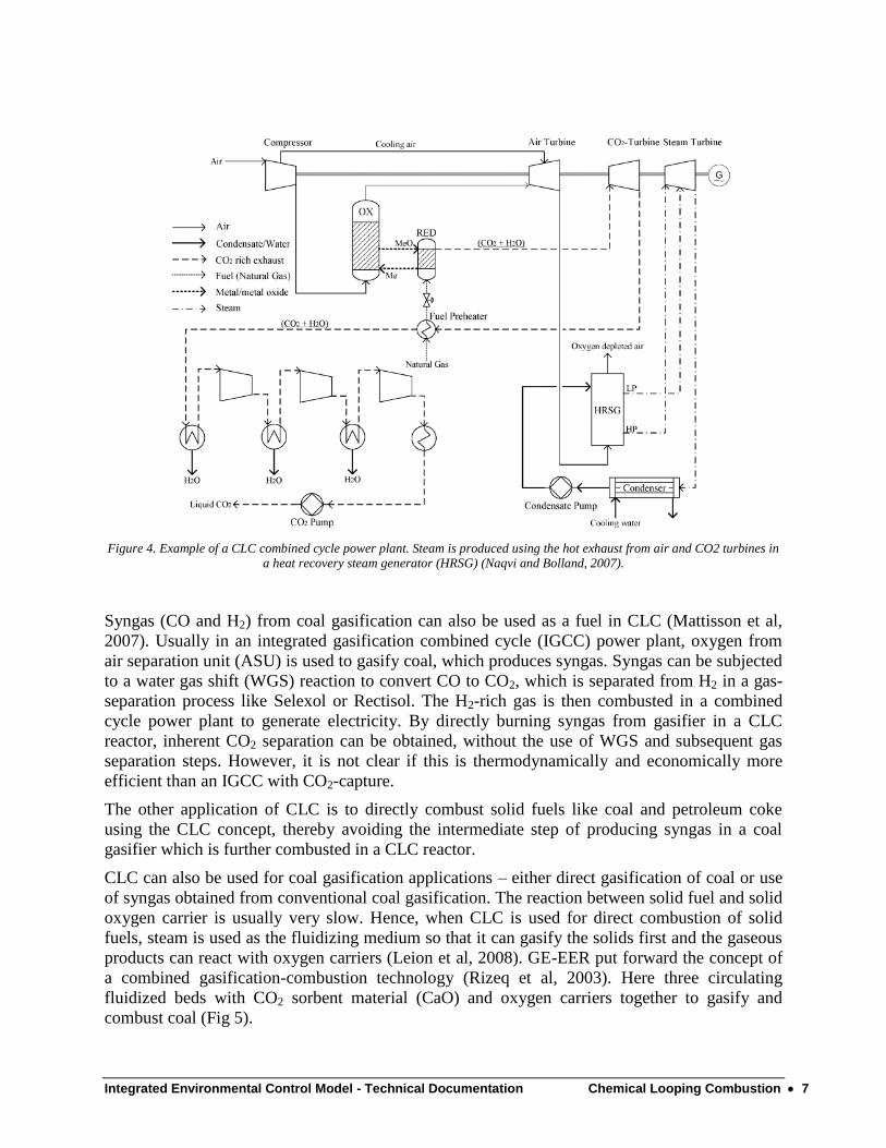
In a variation of this power plant design, Naqvi et al (2006) introduce a heat recovery steam
generator that produces steam from the hot exhaust from the air and CO2 turbines (Fig 4). Being
a combined cycle configuration, this power plant design is more thermally efficient than a simple
cycle design without the steam turbine. The efficiency can further be improved by incorporating
multi chemical-looping reactors which will enable reheating of air in the intermediate stages of
expansion in the air turbine (Naqvi and Bolland, 2007). Though different variations exist in the
particular conceptual plant designs, the common basis is similar to a NGCC power plant with
combustion chamber replaced with a CLC reactor system.
Thermodynamic analyses of CLC combined cycles using natural gas or syngas as fuels found
that the overall efficiencies range from 48 – 55% (lower heating value). Considering that CO2
capture is inherent in this process, this efficiency range is much higher compared to that obtained
from conventional power plants with CCS. However, it must be reiterated that these are only
theoretical studies and it will take much more experimentation with the reactor designs and
oxygen carrier combinations to arrive at a definite conclusion about the feasibility of CLC for
power plant applications. Nevertheless, CLC is a promising technology for power plants with
CO2 capture.
Figure 3. Example of application of CLC to power generation – a simple cycle power plant where hot exhaust from air
(oxidation) and fuel (reduction) reactors are expanded in air and CO2 turbines, respectively (Brandvoll and Bolland, 2004).
Integrated Environmental Control Model - Technical Documentation Chemical Looping Combustion 7
Figure 4. Example of a CLC combined cycle power plant. Steam is produced using the hot exhaust from air and CO2 turbines in
a heat recovery steam generator (HRSG) (Naqvi and Bolland, 2007).
Syngas (CO and H2) from coal gasification can also be used as a fuel in CLC (Mattisson et al,
2007). Usually in an integrated gasification combined cycle (IGCC) power plant, oxygen from
air separation unit (ASU) is used to gasify coal, which produces syngas. Syngas can be subjected
to a water gas shift (WGS) reaction to convert CO to CO2, which is separated from H2 in a gas-
separation process like Selexol or Rectisol. The H2-rich gas is then combusted in a combined
cycle power plant to generate electricity. By directly burning syngas from gasifier in a CLC
reactor, inherent CO2 separation can be obtained, without the use of WGS and subsequent gas
separation steps. However, it is not clear if this is thermodynamically and economically more
efficient than an IGCC with CO2-capture.
The other application of CLC is to directly combust solid fuels like coal and petroleum coke
using the CLC concept, thereby avoiding the intermediate step of producing syngas in a coal
gasifier which is further combusted in a CLC reactor.
CLC can also be used for coal gasification applications – either direct gasification of coal or use
of syngas obtained from conventional coal gasification. The reaction between solid fuel and solid
oxygen carrier is usually very slow. Hence, when CLC is used for direct combustion of solid
fuels, steam is used as the fluidizing medium so that it can gasify the solids first and the gaseous
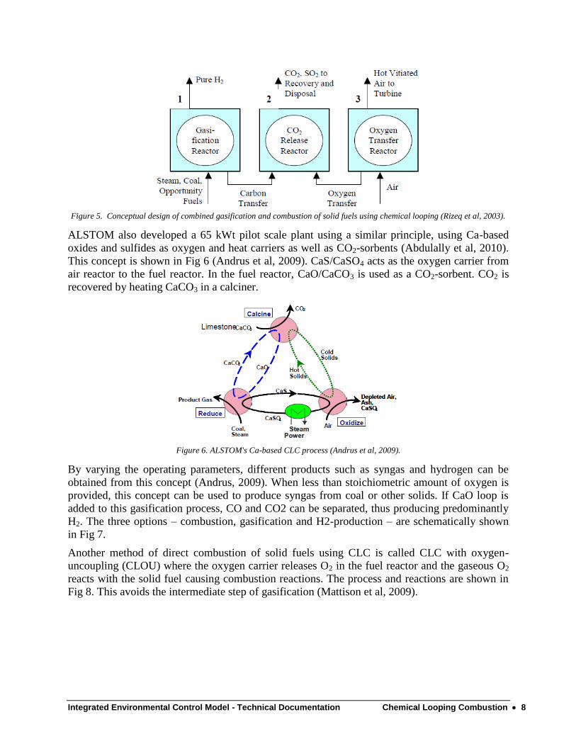
products can react with oxygen carriers (Leion et al, 2008). GE-EER put forward the concept of
a combined gasification-combustion technology (Rizeq et al, 2003). Here three circulating
fluidized beds with CO2 sorbent material (CaO) and oxygen carriers together to gasify and
combust coal (Fig 5).
Integrated Environmental Control Model - Technical Documentation Chemical Looping Combustion 8
Figure 5. Conceptual design of combined gasification and combustion of solid fuels using chemical looping (Rizeq et al, 2003).
ALSTOM also developed a 65 kWt pilot scale plant using a similar principle, using Ca-based
oxides and sulfides as oxygen and heat carriers as well as CO2-sorbents (Abdulally et al, 2010).
This concept is shown in Fig 6 (Andrus et al, 2009). CaS/CaSO4 acts as the oxygen carrier from
air reactor to the fuel reactor. In the fuel reactor, CaO/CaCO3 is used as a CO2-sorbent. CO2 is
recovered by heating CaCO3 in a calciner.
Figure 6. ALSTOM's Ca-based CLC process (Andrus et al, 2009).
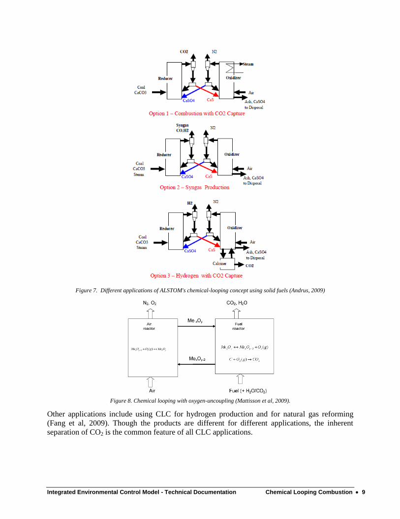
By varying the operating parameters, different products such as syngas and hydrogen can be
obtained from this concept (Andrus, 2009). When less than stoichiometric amount of oxygen is
provided, this concept can be used to produce syngas from coal or other solids. If CaO loop is
added to this gasification process, CO and CO2 can be separated, thus producing predominantly
H2. The three options – combustion, gasification and H2-production – are schematically shown
in Fig 7.
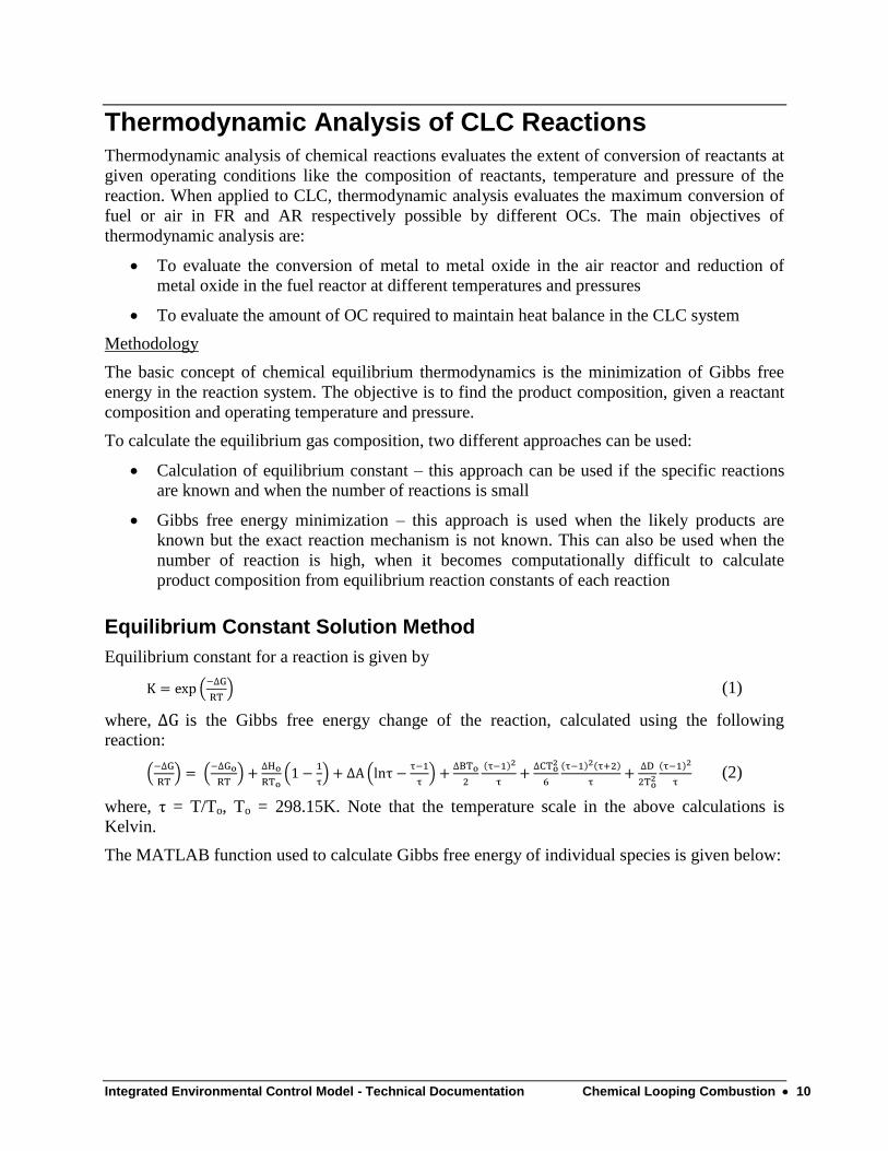
Another method of direct combustion of solid fuels using CLC is called CLC with oxygen-
uncoupling (CLOU) where the oxygen carrier releases O2 in the fuel reactor and the gaseous O2
reacts with the solid fuel causing combustion reactions. The process and reactions are shown in
Fig 8. This avoids the intermediate step of gasification (Mattison et al, 2009).
Integrated Environmental Control Model - Technical Documentation Chemical Looping Combustion 9
Figure 7. Different applications of ALSTOM's chemical-looping concept using solid fuels (Andrus, 2009)
Figure 8. Chemical looping with oxygen-uncoupling (Mattisson et al, 2009).
Other applications include using CLC for hydrogen production and for natural gas reforming
(Fang et al, 2009). Though the products are different for different applications, the inherent
separation of CO2 is the common feature of all CLC applications.
Integrated Environmental Control Model - Technical Documentation Chemical Looping Combustion 10
Thermodynamic Analysis of CLC Reactions Thermodynamic analysis of chemical reactions evaluates the extent of conversion of reactants at
given operating conditions like the composition of reactants, temperature and pressure of the
reaction. When applied to CLC, thermodynamic analysis evaluates the maximum conversion of
fuel or air in FR and AR respectively possible by different OCs. The main objectives of
thermodynamic analysis are:
To evaluate the conversion of metal to metal oxide in the air reactor and reduction of
metal oxide in the fuel reactor at different temperatures and pressures
To evaluate the amount of OC required to maintain heat balance in the CLC system
Methodology
The basic concept of chemical equilibrium thermodynamics is the minimization of Gibbs free
energy in the reaction system. The objective is to find the product composition, given a reactant
composition and operating temperature and pressure.
To calculate the equilibrium gas composition, two different approaches can be used:
Calculation of equilibrium constant – this approach can be used if the specific reactions
are known and when the number of reactions is small
Gibbs free energy minimization – this approach is used when the likely products are
known but the exact reaction mechanism is not known. This can also be used when the
number of reaction is high, when it becomes computationally difficult to calculate
product composition from equilibrium reaction constants of each reaction
Equilibrium Constant Solution Method
Equilibrium constant for a reaction is given by
(1)
where, is the Gibbs free energy change of the reaction, calculated using the following
reaction:
(2)
where, τ = T/To, To = 298.15K. Note that the temperature scale in the above calculations is
Kelvin.
The MATLAB function used to calculate Gibbs free energy of individual species is given below:
Integrated Environmental Control Model - Technical Documentation Chemical Looping Combustion 11
For different reactions, Gibbs free energy change is calculated subtracting the Gibbs free energy
of formation of the reactants from that of the products. For elements, Gibbs free energy is set to
zero. Gibbs free energy of different species is calculated from their formation reactions. The
MATLAB routine used to calculate Gibbs free energy of formation is given below:
where, g_i is the Gibbs free energy of the species calculated using Eqn 2.
For a typical reaction of the form described below, equilibrium concentrations can be calculated
from the equilibrium constant and extent of reaction.
(3)
is the stoichiometric coefficient of the component Ai. The stoichiometric coefficient is
negative for reactants and positive for products.
For a system with multiple reactions, the mole fraction of a given component is given by
(4)
Subscript ‘i' denotes species (total N species) and ‘j’ denotes a particular reaction. The numerator
of the above equation is the number of moles of species ‘i' in the equilibrium mixture and
denominator is the total number of moles of all the species combined in the equilibrium mixture.
(5)
is the extent of reaction ‘j’.
G_CH4 = g_CH4 - G_C-2*G_H2; %C+2H2 -> CH4
G_CO = g_CO-G_C-0.5*G_O2; %C+0.5O2->CO
G_CO2 = g_CO2-G_C-G_O2; %C+O2->CO2
G_H2O = g_H2O-G_H2-0.5*G_O2; %H2+0.5O2->H2O
G_NiO = g_NiO-G_Ni-0.5*G_O2; %Ni+0.5O2->NiO
function G = gibbs(props,T)
%Calculate the Gibbs free energy of a species based on properties
and
%temperature.
%prop_CH4 = [-50460 -74520 1.702 9.081e-3 -2.164e-6 0];
g = props(1);
h = props(2);
A = props(3);
B = props(4);
C = props(5);
D = props(6);
G = -8.314*T*(-g/(8.314*298.15)+h/(8.314*298.15)*(1-298.15/T)+...
A*(log(T/298.15)-1+298.15/T)+...
(B/2)*298.15*(T/298.15-1)^2/(T/298.15)+ ...
(C/6)*298.15^2*(T/298.15-1)^2*(T/298.15+2)/(T/298.15) ...
+(D/2)*(T/298.15-1)^2/T^2);
Integrated Environmental Control Model - Technical Documentation Chemical Looping Combustion 12
Equilibrium constant of each reaction can be defined as
(6)
K can be calculated at any given temperature using eqns 1 and 2. By writing these equations for
all reactions and species, we get a series of linear equations as a function of extent of reaction
( ). These can be solved numerically and the equilibrium concentrations of each species can be
calculated.
Adiabatic Temperature
When the reaction occurs under adiabatic conditions, no heat is lost to the surroundings and
hence, the temperature of the products increases for an exothermic reaction. The process can be
thought of as occurring at standard temperature (298.15K) and then heating of the products from
standard temperature to the final temperature. Since no heat is lost, the whole heat of reaction is
used to heat up the products.
(7)
(8)
(9)
The values of constants A, B, C and D for different species are obtained from standard property
tables. Properties of some of the materials relevant to CLC are shown in Table 1.
The MATLAB function to calculate specific heat is given below:
The overall Cp of the mixture of gases is obtained by multiplying the individual specific heats
with the respective mole fractions of each species. Cp also depends on temperature, so an
iterative solution is required to calculate the adiabatic reaction temperature. Also, the heat carried
into any reactor depends on the flow rates and temperatures of different inlet components.
function C_p = spec_heat(props,T)
%Calculate the specific heat based on properties
%prop_CH4 = [-50460 -74520 1.702 9.081e-3 -2.164e-6 0];
A = props(3);
B = props(4);
C = props(5);
D = props(6);
C_p = 8.314*(A+B*298.15*(T/298.15+1)/2+ ...
C*298.15^2*((T/298.15)^2+(T/298.15)+1)/3 ...
+D/(T*298.15));
Integrated Environmental Control Model - Technical Documentation Chemical Looping Combustion 13
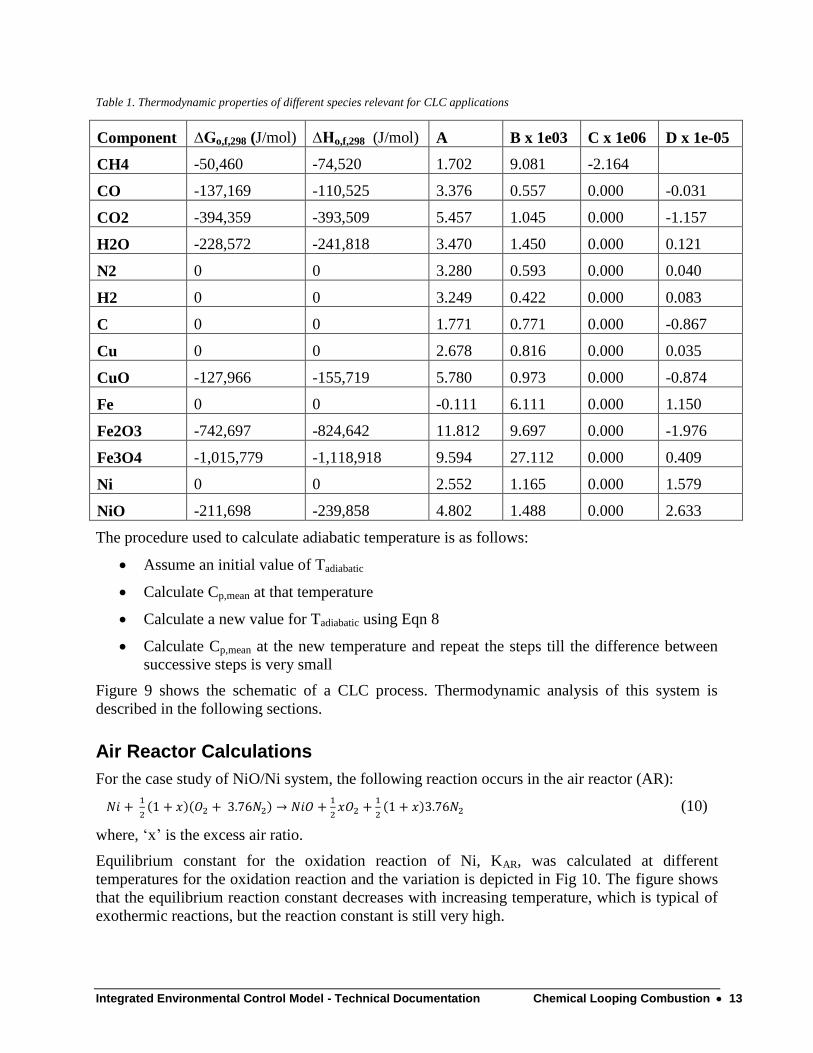
Table 1. Thermodynamic properties of different species relevant for CLC applications
Component ∆Go,f,298 (J/mol) ∆Ho,f,298 (J/mol) A B x 1e03 C x 1e06 D x 1e-05
CH4 -50,460 -74,520 1.702 9.081 -2.164
CO -137,169 -110,525 3.376 0.557 0.000 -0.031
CO2 -394,359 -393,509 5.457 1.045 0.000 -1.157
H2O -228,572 -241,818 3.470 1.450 0.000 0.121
N2 0 0 3.280 0.593 0.000 0.040
H2 0 0 3.249 0.422 0.000 0.083
C 0 0 1.771 0.771 0.000 -0.867
Cu 0 0 2.678 0.816 0.000 0.035
CuO -127,966 -155,719 5.780 0.973 0.000 -0.874
Fe 0 0 -0.111 6.111 0.000 1.150
Fe2O3 -742,697 -824,642 11.812 9.697 0.000 -1.976
Fe3O4 -1,015,779 -1,118,918 9.594 27.112 0.000 0.409
Ni 0 0 2.552 1.165 0.000 1.579
NiO -211,698 -239,858 4.802 1.488 0.000 2.633
The procedure used to calculate adiabatic temperature is as follows:
Assume an initial value of Tadiabatic
Calculate Cp,mean at that temperature
Calculate a new value for Tadiabatic using Eqn 8
Calculate Cp,mean at the new temperature and repeat the steps till the difference between
successive steps is very small
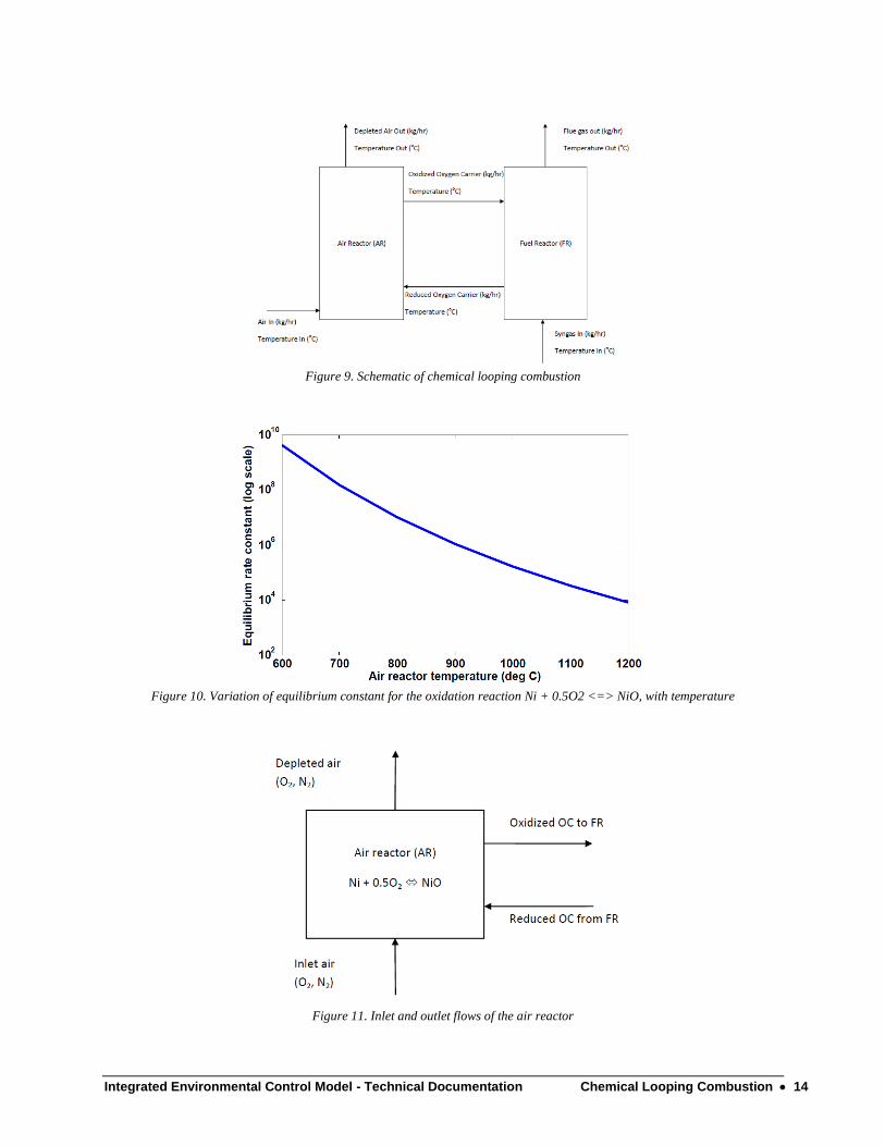
Figure 9 shows the schematic of a CLC process. Thermodynamic analysis of this system is
described in the following sections.
Air Reactor Calculations
For the case study of NiO/Ni system, the following reaction occurs in the air reactor (AR):
(10)
where, ‘x’ is the excess air ratio.
Equilibrium constant for the oxidation reaction of Ni, KAR, was calculated at different
temperatures for the oxidation reaction and the variation is depicted in Fig 10. The figure shows
that the equilibrium reaction constant decreases with increasing temperature, which is typical of
exothermic reactions, but the reaction constant is still very high.
Integrated Environmental Control Model - Technical Documentation Chemical Looping Combustion 14
Figure 9. Schematic of chemical looping combustion
Figure 10. Variation of equilibrium constant for the oxidation reaction Ni + 0.5O2 <=> NiO, with temperature
Figure 11. Inlet and outlet flows of the air reactor
Integrated Environmental Control Model - Technical Documentation Chemical Looping Combustion 15
Figure 11 shows the mass flows for the air reactor. Inlet air and the reduced form of OC
(predominantly Ni) enter the air reactor where the oxidation reaction takes place. The extent of
the reaction depends on the temperature at which it takes place. The amount of O2 at equilibrium
conditions can be calculated using the equilibrium constant in the following way
(11)
yO2 is the mole fraction of O2 at equilibrium conditions. Since Ni and NiO are solids, their
amounts are included in the equilibrium constant equation. Since the reaction constant is
inversely proportional to the mole fraction of oxygen (eqn 11), it can be safely assumed that the
oxidation reaction goes to completion, i.e almost zero amount of oxygen is present under
equilibrium conditions. Hence, the mass balance equations can be written using simple
stoichiometry for the air reactor. The following equations, expressed in molar terms for
simplicity, are used to calculate the mass balance in the AR.
Inlet flows
Mair,in = (1+x)Mair,stoichiometric (12)
MO2,in = 0.21Mair,in (13)
MN2,in = 0.79Mair,in (14)
The oxygen carrier consists of Ni, NiO and an inert material used to support the metal oxide as
well as increase the surface area of reaction. The support material considered here is Al2O3.
Oxygen carrier consisting of 40% MeO and 60% Al2O3 has been widely tested at lab-scale
[Abad et al, 2007]. This inert material does not undergo any reaction and so its mass does not
change throughout the system. The mass fraction of MeO in the OC is denoted by xMeO. Ideally,
stoichiometric amount of NiO is needed for the combustion reaction of fuel and hence no NiO is
present at the outlet of the fuel reactor and hence in the inlet to the air reactor. But extra NiO
may be present in order to carry sufficient heat between the two reactors. The excess NiO at the
AR inlet (which is FR outlet) is represented as the fraction ‘z’, which is the molar ratio of NiO to
OC.
z = MNiO/(MNiO + MNi) (15)
When ‘z’ is zero, there is no NiO in the inlet. When z = 1, which is not a possible condition,
there is no Ni in the inlet stream of the AR.
MNi,in = MNi,out,FR
MNiO,in = MNiO,out,FR = z/(1-z) MNi,in (16)
xMeO = MNiO x MWNiO/ (MNiO x MWNiO + MAl2O3 x MWAl2O3)
MAl2O3 = (1-xMeO)/xMeO x (MWNiO/MWAl2O3) x MNiO (17)
It has to be noted that xMeO is the fraction of NiO in fully oxidized OC.
Outlet flows
One mole of Ni reacts with 0.5 moles of O2 to form one mole of NiO. Hence outlet flow of O2
can be calculated as
MO2,out = MO2,in – 0.5MNi,in (18)
Integrated Environmental Control Model - Technical Documentation Chemical Looping Combustion 16
Nitrogen does not participate in the reactions. Hence, its inlet and outlet flows are the same.
MN2,out = MN2,in
Mair,out = MO2,out + MN2,out (19)
Since in most practical applications, there will be some amount of excess air, it can be assumed
that all of Ni is oxidized to NiO. One mole of Ni is converted to one mole of NiO.
MNi,out = 0 (20)
MNiO,out = MNiO,in + MNi,in = 1/(1-z)MNi,in (21)
Adiabatic temperature of AR
Assuming one mole of Ni at the inlet to AR, all other flows are expressed per mole of Ni. O2
mole flow is also expressed in terms of excess air ratio ‘x’ and NiO mole flow is a function of
‘z’. For CLC applications in IGCC, the most suitable approach will be to operate the CLC
system at the gas turbine pressure since depleted air from the AR will be the motive fluid in the
gas turbine. Hence, inlet air to the AR needs to be compressed to that pressure. Inlet temperature
of air to AR is the same as the compressor exit temperature. Reduced OC coming from the FR is
of the same temperature as the FR. Tair and TMeO are the temperatures of inlet air and MeO,
respectively. Thus, adiabatic temperature can be calculated as a function of ‘x’, ‘z’, Tair and
TMeO.
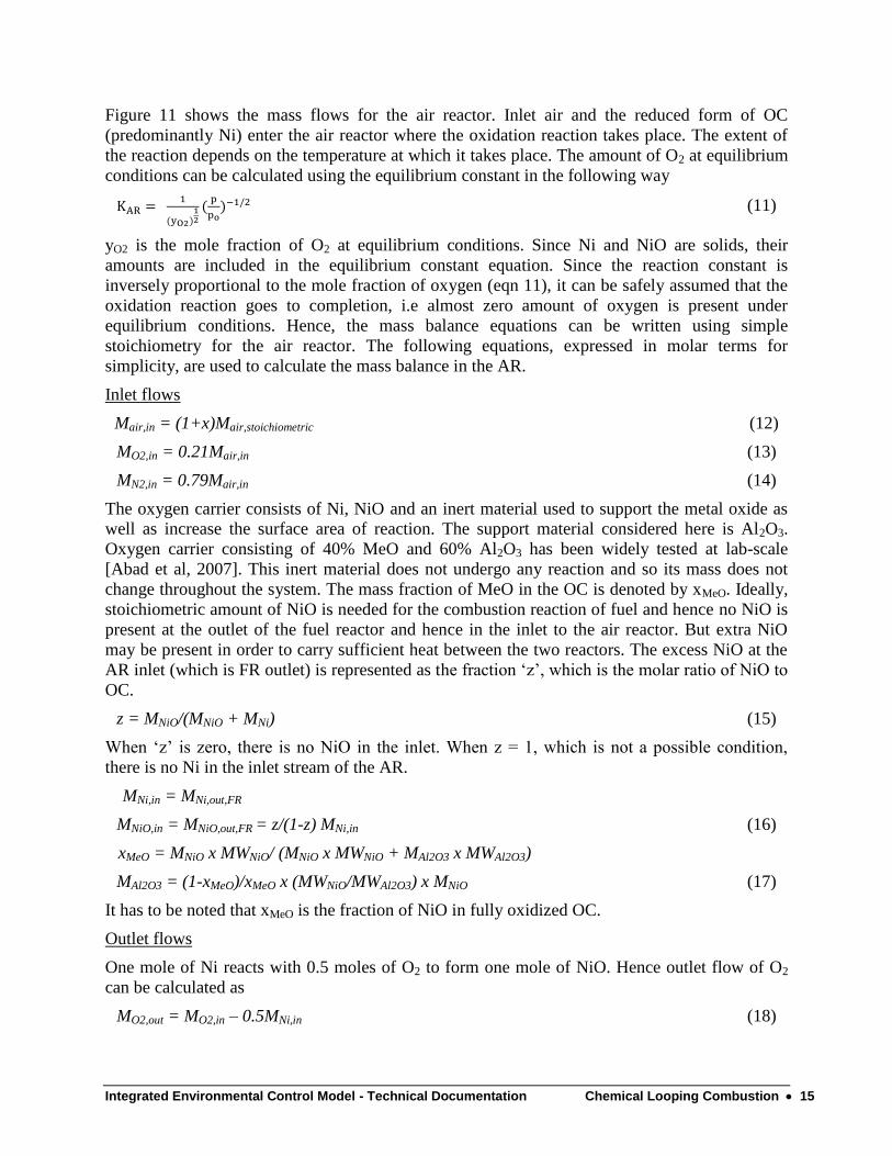
The heat released in the reaction is called heat of reaction. The heat of reaction for the oxidation
reaction of Ni at different temperatures is shown in Fig 12. It can be seen that the heat of reaction
decreases with temperature, but only marginally.
Figure 12. Variation of heat of reaction of Ni + 0.5O2 NiO, with temperature
Integrated Environmental Control Model - Technical Documentation Chemical Looping Combustion 17
The MATLAB routine to calculate the adiabatic temperature is given below:
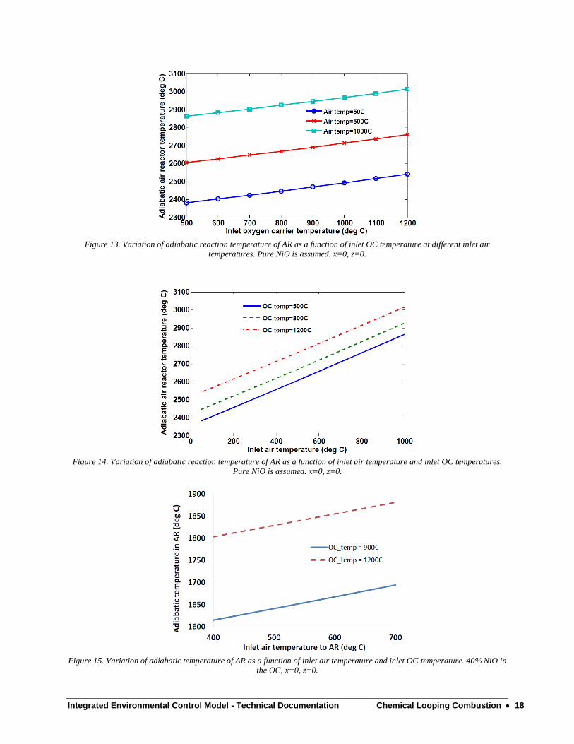
Figure 13 shows the variation of adiabatic reaction temperature of AR as a function of inlet OC
temperature at different inlet air temperatures, when there is no excess air or NiO. Similarly, Fig
14 shows the variation with inlet air temperature at different OC temperatures. Pure NiO, without
any support material, is considered for these calculations. For no excess air or NiO, adiabatic
temperature in the AR is extremely high, much higher than the melting points of most of the
metals. Thus, there is a need for support materials in order to enhance the thermal stability of the
OCs. Excess air and MeO also help in carrying away some heat of reaction thereby reducing the
adiabatic temperature.
Figure 15 shows the same variation with a supported OC (40% NiO, 60% Al2O3). It can be
observed that the adiabatic temperature has decreased considerably compared to a pure NiO
oxygen carrier. This temperature is still higher than the melting point of NiO (1200oC).
%%%%% Calculating adiabatic reaction temperature
H_reactants = H_R_sens+H_Reaction_298;
for m=1:length(T_air)
for n=1:length(T_MeO)
num=H_reactants(m,n);
T_adia(1) = 600; %K, initial guess
for k=2:100
T = T_adia(k-1);
props = prop_Ni;
C_p_Ni = spec_heat(props,T);
props = prop_O2;
C_p_O2 = spec_heat(props,T);
props = prop_N2;
C_p_N2 = spec_heat(props,T);
props = prop_NiO;
C_p_NiO = spec_heat(props,T);
props=prop_Al2O3;
C_p_Al2O3=spec_heat(props,T);
denom = 1000*(M_Ni_out*C_p_Ni+M_O2_out*C_p_O2+...
M_N2_out*C_p_N2+M_NiO_out*C_p_NiO+M_Al2O3_out*C_p_Al2O3);
T_adia(k)=298.15-num/denom;
err = abs(T_adia(k)-T_adia(k-1));
T_out(m,n)=T_adia(k)-273.15;
if err<1, break; end
end
end
end
Integrated Environmental Control Model - Technical Documentation Chemical Looping Combustion 18
Figure 13. Variation of adiabatic reaction temperature of AR as a function of inlet OC temperature at different inlet air
temperatures. Pure NiO is assumed. x=0, z=0.
Figure 14. Variation of adiabatic reaction temperature of AR as a function of inlet air temperature and inlet OC temperatures.
Pure NiO is assumed. x=0, z=0.
Figure 15. Variation of adiabatic temperature of AR as a function of inlet air temperature and inlet OC temperature. 40% NiO in
the OC, x=0, z=0.
Integrated Environmental Control Model - Technical Documentation Chemical Looping Combustion 19
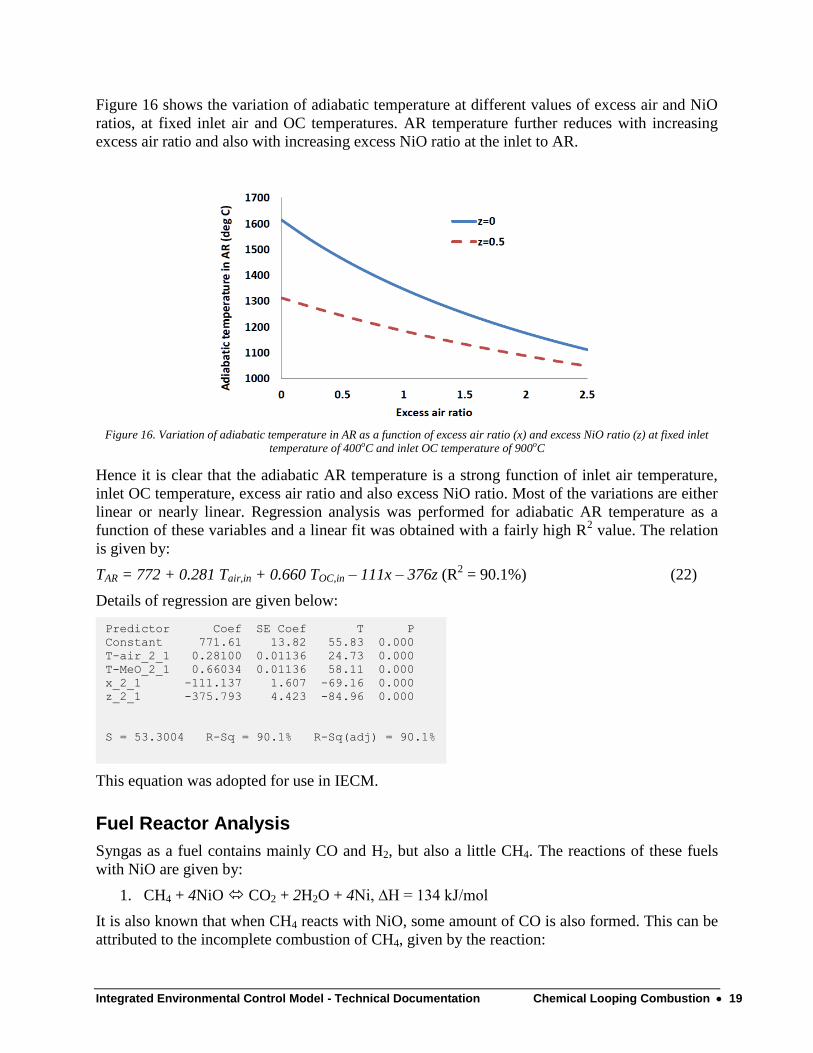
Figure 16 shows the variation of adiabatic temperature at different values of excess air and NiO
ratios, at fixed inlet air and OC temperatures. AR temperature further reduces with increasing
excess air ratio and also with increasing excess NiO ratio at the inlet to AR.
Figure 16. Variation of adiabatic temperature in AR as a function of excess air ratio (x) and excess NiO ratio (z) at fixed inlet
temperature of 400oC and inlet OC temperature of 900oC
Hence it is clear that the adiabatic AR temperature is a strong function of inlet air temperature,
inlet OC temperature, excess air ratio and also excess NiO ratio. Most of the variations are either
linear or nearly linear. Regression analysis was performed for adiabatic AR temperature as a
function of these variables and a linear fit was obtained with a fairly high R2 value. The relation
is given by:
TAR = 772 + 0.281 Tair,in + 0.660 TOC,in – 111x – 376z (R2 = 90.1%) (22)
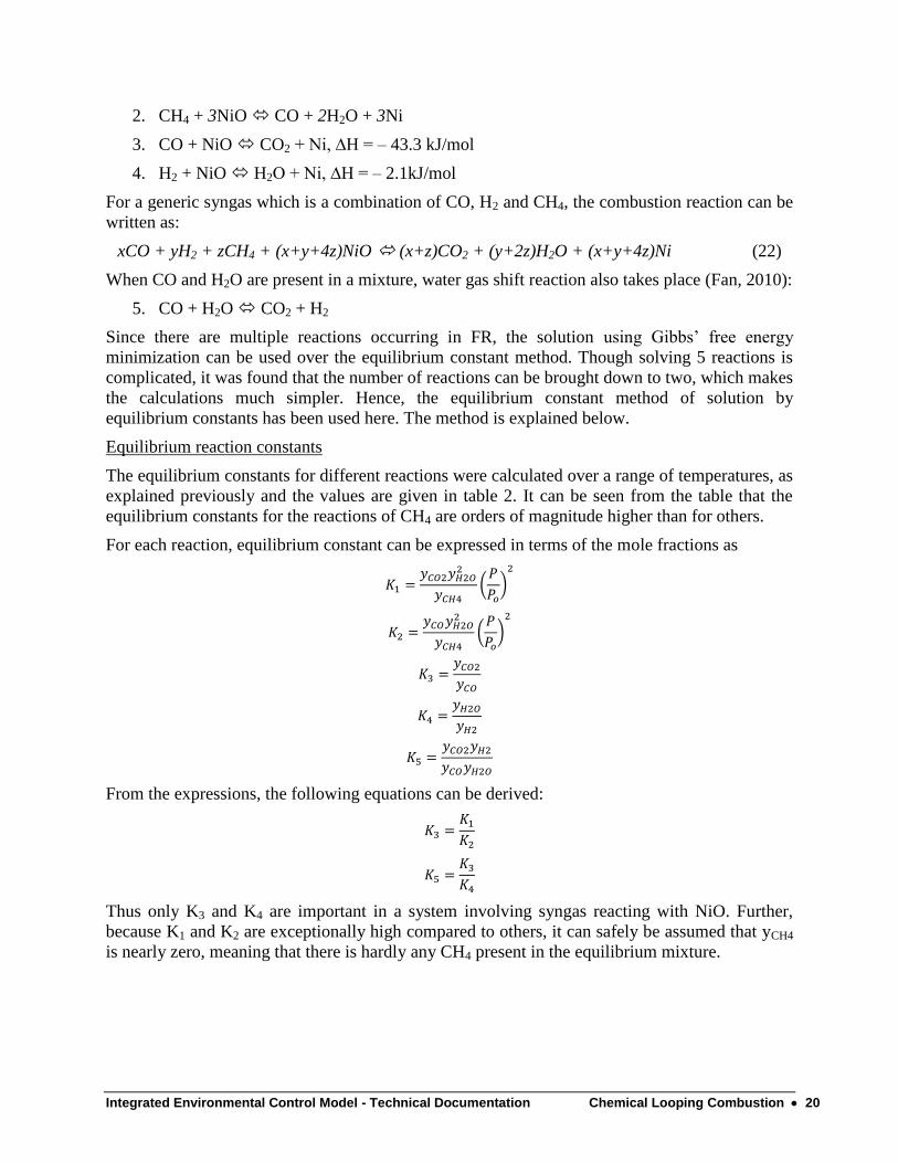
Details of regression are given below:
This equation was adopted for use in IECM.
Fuel Reactor Analysis
Syngas as a fuel contains mainly CO and H2, but also a little CH4. The reactions of these fuels
with NiO are given by:
1. CH4 + 4NiO CO2 + 2H2O + 4Ni, ∆H = 134 kJ/mol
It is also known that when CH4 reacts with NiO, some amount of CO is also formed. This can be
attributed to the incomplete combustion of CH4, given by the reaction:
Predictor Coef SE Coef T P
Constant 771.61 13.82 55.83 0.000
T-air_2_1 0.28100 0.01136 24.73 0.000
T-MeO_2_1 0.66034 0.01136 58.11 0.000
x_2_1 -111.137 1.607 -69.16 0.000
z_2_1 -375.793 4.423 -84.96 0.000
S = 53.3004 R-Sq = 90.1% R-Sq(adj) = 90.1%
Integrated Environmental Control Model - Technical Documentation Chemical Looping Combustion 20
2. CH4 + 3NiO CO + 2H2O + 3Ni
3. CO + NiO CO2 + Ni, ∆H = – 43.3 kJ/mol
4. H2 + NiO H2O + Ni, ∆H = – 2.1kJ/mol
For a generic syngas which is a combination of CO, H2 and CH4, the combustion reaction can be
written as:
xCO + yH2 + zCH4 + (x+y+4z)NiO (x+z)CO2 + (y+2z)H2O + (x+y+4z)Ni (22)
When CO and H2O are present in a mixture, water gas shift reaction also takes place (Fan, 2010):
5. CO + H2O CO2 + H2
Since there are multiple reactions occurring in FR, the solution using Gibbs’ free energy
minimization can be used over the equilibrium constant method. Though solving 5 reactions is
complicated, it was found that the number of reactions can be brought down to two, which makes
the calculations much simpler. Hence, the equilibrium constant method of solution by
equilibrium constants has been used here. The method is explained below.
Equilibrium reaction constants
The equilibrium constants for different reactions were calculated over a range of temperatures, as
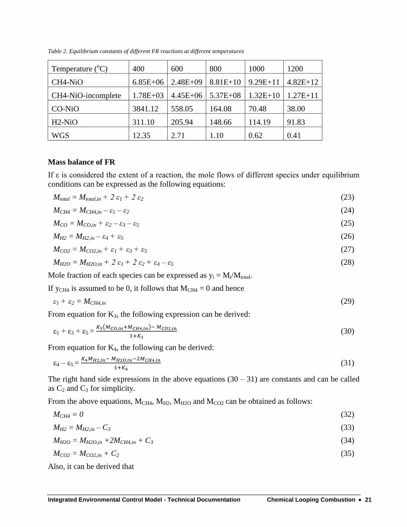
explained previously and the values are given in table 2. It can be seen from the table that the
equilibrium constants for the reactions of CH4 are orders of magnitude higher than for others.
For each reaction, equilibrium constant can be expressed in terms of the mole fractions as
From the expressions, the following equations can be derived:
Thus only K3 and K4 are important in a system involving syngas reacting with NiO. Further,
because K1 and K2 are exceptionally high compared to others, it can safely be assumed that yCH4
is nearly zero, meaning that there is hardly any CH4 present in the equilibrium mixture.
Integrated Environmental Control Model - Technical Documentation Chemical Looping Combustion 21
Table 2. Equilibrium constants of different FR reactions at different temperatures
Temperature (oC) 400 600 800 1000 1200
CH4-NiO 6.85E+06 2.48E+09 8.81E+10 9.29E+11 4.82E+12
CH4-NiO-incomplete 1.78E+03 4.45E+06 5.37E+08 1.32E+10 1.27E+11
CO-NiO 3841.12 558.05 164.08 70.48 38.00
H2-NiO 311.10 205.94 148.66 114.19 91.83
WGS 12.35 2.71 1.10 0.62 0.41
Mass balance of FR
If ε is considered the extent of a reaction, the mole flows of different species under equilibrium
conditions can be expressed as the following equations:
Mtotal = Mtotal,in + 2 ε1 + 2 ε2 (23)
MCH4 = MCH4,in – ε1 – ε2 (24)
MCO = MCO,in + ε2 – ε3 – ε5 (25)
MH2 = MH2,in – ε4 + ε5 (26)
MCO2 = MCO2,in + ε1 + ε3 + ε5 (27)
MH2O = MH2O,in + 2 ε1 + 2 ε2 + ε4 – ε5 (28)
Mole fraction of each species can be expressed as yi = Mi/Mtotal.
If yCH4 is assumed to be 0, it follows that MCH4 = 0 and hence
ε1 + ε2 = MCH4,in (29)
From equation for K3, the following expression can be derived:
ε1 + ε3 + ε5 =
(30)
From equation for K4, the following can be derived:
ε4 – ε5 =
(31)
The right hand side expressions in the above equations (30 – 31) are constants and can be called
as C2 and C3 for simplicity.
From the above equations, MCH4, MH2, MH2O and MCO2 can be obtained as follows:
MCH4 = 0 (32)
MH2 = MH2,in – C3 (33)
MH2O = MH2O,in +2MCH4,in + C3 (34)
MCO2 = MCO2,in + C2 (35)
Also, it can be derived that
Integrated Environmental Control Model - Technical Documentation Chemical Looping Combustion 22
MCO2 + MCO = MCO2,in + MCO,in + MCH4,in – C3
Hence, expression for MCO can also be obtained:
MCO = MCO,in + MCH4,in – C2 (36)
Mtotal = Mtotal,in + 2MCH4,in (37)
Hence mole flows of all the reacting components can be obtained by the above algebraic
expressions (32 – 37). The constants C2 and C3 are functions of equilibrium constants K3 and K4,
which are a function of temperature. Thus, mass balance can be solved for any given
temperature. The mole flows of other components in the syngas such as N2, Ar etc remain
unchanged since they don’t take part in any reaction.
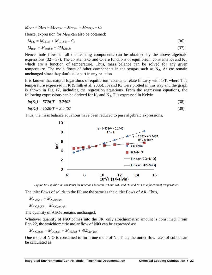
It is known that natural logarithms of equilibrium constants relate linearly with 1/T, where T is
temperature expressed in K (Smith et al, 2005). K3 and K4 were plotted in this way and the graph
is shown in Fig 17, including the regression equations. From the regression equations, the
following expressions can be derived for K3 and K4, T is expressed in Kelvin:
ln(K3) = 5726/T – 0.2407 (38)
ln(K4) = 1520/T + 3.5467 (39)
Thus, the mass balance equations have been reduced to pure algebraic expressions.
Figure 17. Equilibrium constants for reactions between CO and NiO and H2 and NiO as a function of temperature
The inlet flows of solids to the FR are the same as the outlet flows of AR. Thus,
MNi,in,FR = MNi,out,AR
MNiO,in,FR = MNiO,out,AR
The quantity of Al2O3 remains unchanged.
Whatever quantity of NiO comes into the FR, only stoichiometric amount is consumed. From
Eqn 22, the stoichiometric molar flow of NiO can be expressed as:
MNiO,stoic = MCO,fuel + MH2,fuel + 4MCH4,fuel
One mole of NiO is consumed to form one mole of Ni. Thus, the outlet flow rates of solids can
be calculated as:
Integrated Environmental Control Model - Technical Documentation Chemical Looping Combustion 23
MNiO,out,FR = MNiO,in,FR – MNiO,stoic (40)
MNi,out,FR = MNi,in,FR + MNiO,stoic (41)
Thus, both the solids and gases’ mass flow has been accounted for.
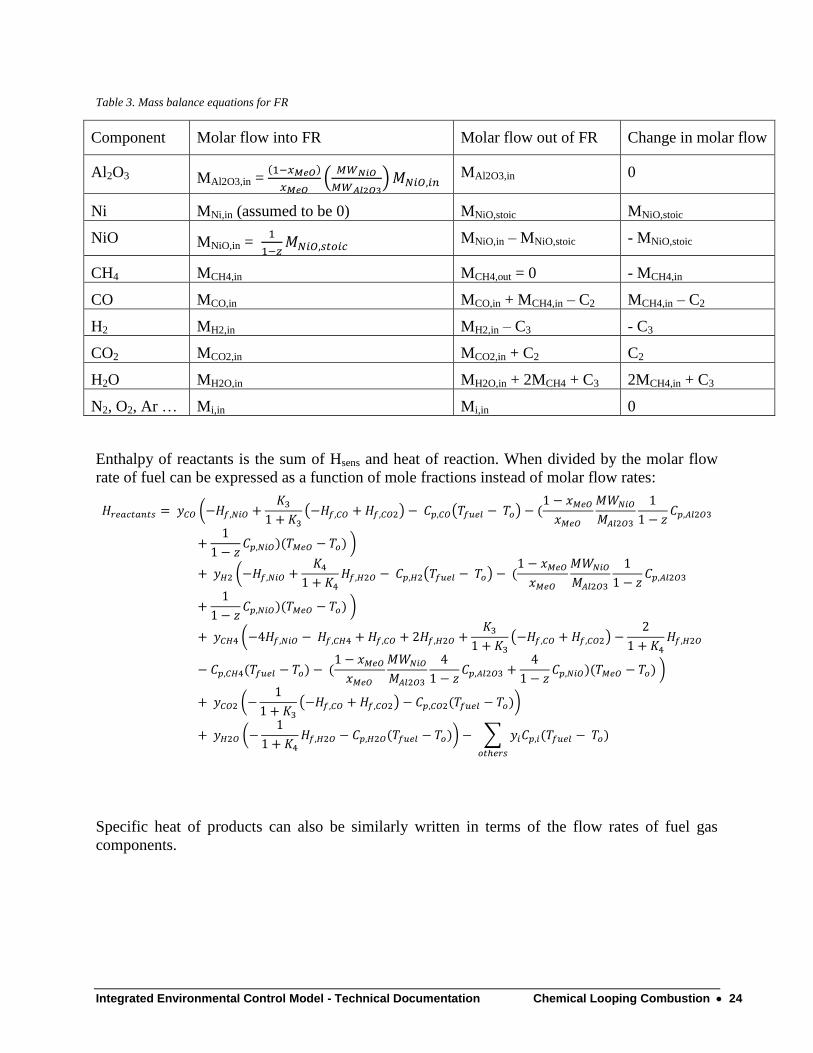
Mass balance equations for FR are summarized in Table 3.
Adiabatic temperature of FR
Because of temperature dependence of specific heat, an iterative procedure is required to
calculate adiabatic temperature from Eqn 8. However, a simplified solution is developed here
which avoids the use of interative calculations.
Heat of reaction at 298.15K can be written as
Using expressions from the above table and substituting expressions for MNiO,stoic from Eqn
22 and C2 and C3 from eqns 30 and 31, heat of reaction can be expressed in terms of inlet molar
flows or mole fractions.
The reactants (fuel and OC) are at a higher temperature than 298.15K. For calculation, it is
assumed that the reactants are cooled to 298.15K, at which temperature the reaction takes place
and the products are heated to the adiabatic temperature. So the sensible heat of cooling of
reactants has to be accounted for.
Integrated Environmental Control Model - Technical Documentation Chemical Looping Combustion 24
Table 3. Mass balance equations for FR
Component Molar flow into FR Molar flow out of FR Change in molar flow
Al2O3 MAl2O3,in =
MAl2O3,in 0
Ni MNi,in (assumed to be 0) MNiO,stoic MNiO,stoic
NiO MNiO,in =
MNiO,in – MNiO,stoic - MNiO,stoic
CH4 MCH4,in MCH4,out = 0 - MCH4,in
CO MCO,in MCO,in + MCH4,in – C2 MCH4,in – C2
H2 MH2,in MH2,in – C3 - C3
CO2 MCO2,in MCO2,in + C2 C2
H2O MH2O,in MH2O,in + 2MCH4 + C3 2MCH4,in + C3
N2, O2, Ar … Mi,in Mi,in 0
Enthalpy of reactants is the sum of Hsens and heat of reaction. When divided by the molar flow
rate of fuel can be expressed as a function of mole fractions instead of molar flow rates:
Specific heat of products can also be similarly written in terms of the flow rates of fuel gas
components.
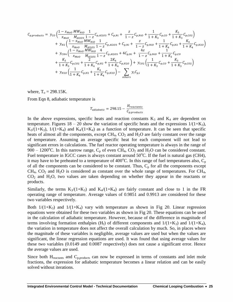
Integrated Environmental Control Model - Technical Documentation Chemical Looping Combustion 25
where, To = 298.15K.
From Eqn 8, adiabatic temperature is
In the above expressions, specific heats and reaction constants K3 and K4 are dependent on
temperature. Figures 18 – 20 show the variation of specific heats and the expressions 1/(1+K3),
K3/(1+K3), 1/(1+K4) and K4/(1+K4) as a function of temperature. It can be seen that specific
heats of almost all the components, except CH4, CO2 and H2O are fairly constant over the range
of temperature. Assuming an average specific heat for each component will not lead to
significant errors in calculations. The fuel reactor operating temperature is always in the range of
900 – 1200oC. In this narrow range, Cp of even CH4, CO2 and H2O can be considered constant.
Fuel temperature in IGCC cases is always constant around 50oC. If the fuel is natural gas (CH4),
it may have to be preheated to a temperature of 400oC. In this range of fuel temperatures also, Cp
of all the components can be considered to be constant. Thus, Cp for all the components except
CH4, CO2 and H2O is considered as constant over the whole range of temperatures. For CH4,
CO2 and H2O, two values are taken depending on whether they appear in the reactants or
products.
Similarly, the terms K3/(1+K3) and K4/(1+K4) are fairly constant and close to 1 in the FR
operating range of temperature. Average values of 0.9851 and 0.9913 are considered for these
two variables respectively.
Both 1/(1+K3) and 1/(1+K4) vary with temperature as shown in Fig 20. Linear regression
equations were obtained for these two variables as shown in Fig 20. These equations can be used
in the calculation of adiabatic temperature. However, because of the difference in magnitude of
terms involving formation enthalpies (Hf) of different components and 1/(1+K3) and 1/(1+K4),
the variation in temperature does not affect the overall calculation by much. So, in places where
the magnitude of these variables is negligible, average values are used but when the values are
significant, the linear regression equations are used. It was found that using average values for
these two variables (0.0149 and 0.0087 respectively) does not cause a significant error. Hence
the average values are used.
Since both Hreactants and Cp,products can now be expressed in terms of constants and inlet mole
fractions, the expression for adiabatic temperature becomes a linear relation and can be easily
solved without iterations.
Integrated Environmental Control Model - Technical Documentation Chemical Looping Combustion 26
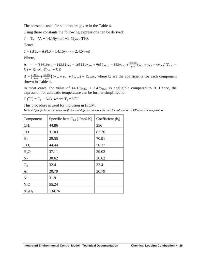
The constants used for solution are given in the Table 4.
Using these constants the following expressions can be derived:
T = To – (A + 14.15yCO2T +2.42yH2OT)/B
Hence,
T = (BTo – A)/(B + 14.15yCO2 + 2.42yH2O)
Where,
A =
B =
, where bi are the coefficients for each component
shown in Table 4.
In most cases, the value of 14.15yCO2 + 2.42yH2O is negligible compared to B. Hence, the
expression for adiabatic temperature can be further simplified to:
T (oC) = To – A/B, where To =25
oC.
This procedure is used for inclusion in IECM.
Table 4. Specific heats and other coefficients of different components used for calculation of FR adiabatic temperature
Component Specific heat Cp,i (J/mol-K) Coefficient (bi)
CH4 44.86 256
CO 31.03 82.26
H2 29.55 70.91
CO2 44.44 50.37
H2O 37.11 39.02
N2 30.62 30.62
O2 32.4 32.4
Ar 20.79 20.79
Ni 31.9
NiO 55.24
Al2O3 134.76
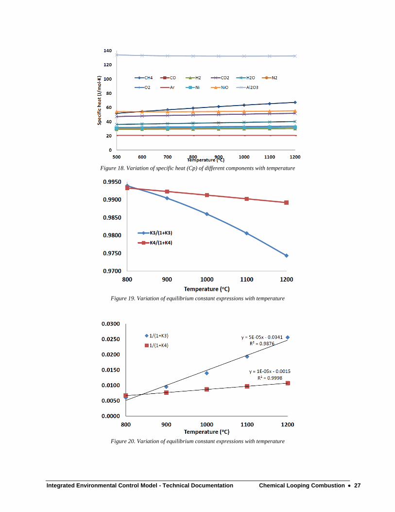
Integrated Environmental Control Model - Technical Documentation Chemical Looping Combustion 27
Figure 18. Variation of specific heat (Cp) of different components with temperature
Figure 19. Variation of equilibrium constant expressions with temperature
Figure 20. Variation of equilibrium constant expressions with temperature
Integrated Environmental Control Model - Technical Documentation Chemical Looping Combustion 28
Alternative method to calculate adiabatic temperature of FR
The adiabatic temperature of FR can also be calculated in a manner similar to that explained for
AR. Adiabatic temperature depends on the inlet composition and temperature of fuel, OC and
their mass flow rates, by using regression analysis for TFR in terms of inlet composition and
temperatures. However, since the number of components in inlet syngas is much higher than in
air, regression equations can be developed for fixed syngas compositions.
As case studies, three different fuel compositions are considered – syngas derived from Illinois#6
coal using GE, E-Gas and Shell gasification technologies (NETL, 2007a).
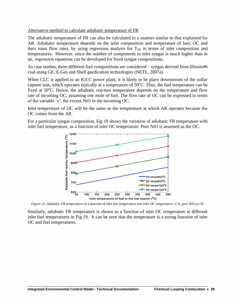
When CLC is applied to an IGCC power plant, it is likely to be place downstream of the sulfur
capture unit, which operates typically at a temperature of 50oC. Thus, the fuel temperature can be
fixed at 50oC. Hence, the adiabatic reaction temperature depends on the temperature and flow
rate of incoming OC, assuming one mole of fuel. The flow rate of OC can be expressed in terms
of the variable ‘z’, the excess NiO in the incoming OC.
Inlet temperature of OC will be the same as the temperature at which AR operates because the
OC comes from the AR.
For a particular syngas composition, Fig 18 shows the variation of adiabatic FR temperature with
inlet fuel temperature, as a function of inlet OC temperature. Pure NiO is assumed as the OC.
Figure 21. Adiabatic FR temperature as a function of inlet fuel temperature and inlet OC temperature. z=0, pure NiO as OC
Similarly, adiabatic FR temperature is shown as a function of inlet OC temperature at different
inlet fuel temperatures in Fig 19. It can be seen that the temperature is a strong function of inlet
OC and fuel temperatures.
Integrated Environmental Control Model - Technical Documentation Chemical Looping Combustion 29
Figure 22. Adiabatic FR temperature as a function of inlet OC temperature and inlet fuel temperatures. z=0, pure NiO as OC
Figure 20 shows the variation in FR temperature with excess NiO in the inlet (z) for three
different gasification technologies. OC inlet temperature is 1200oC. The temperature is a strong
function of excess NiO for all three cases.
Figure 23. Adiabatic fuel reactor temperature as a function of excess NiO (z) at inlet OC temperature = 1200oC. xMeO = 40%
Regression analysis was performed for FR adiabatic temperature as a function of variables inlet
OC temperature and excess NiO. The results showed a fairly strong linear relation with R2 values
nearly equal to 1. The equations for different gasification cases are as follows:
TFR = 61.3 + 56z + 0.891TOC, for GE case (R2 = 99.7%) (41)
TFR = 19.4 + 95.7z + 0.891TOC, for E-Gas case (R2 = 99.6%) (42)
TFR = 102 + 8.06z + 0.9TOC, for the Shell case (R2 = 99.7%) (43)
Thus, adiabatic temperature of FR can be calculated once AR temperature and z are fixed. This
method, however, has not been used in IECM since the earlier method is more robust and can be
adapted to any inlet composition or temperatures.
Integrated Environmental Control Model - Technical Documentation Chemical Looping Combustion 30
Methods for Calculating Solids Inventory
Two important variables in the design of a CLC system are the solids circulation rate and solids
inventory. Solids circulation rate is determined by the amount of oxygen that needs to be
transferred between the reactors and also to cater to the heat balance of the system. The mass
balance analysis described before calculates the mass and molar flow rate of solids between the
two reactors. Two methods are presented here to calculate solids inventory in the system.
Method 1
Inventory of solids in each reactor depends on the reactivity of the OC with fuel and air, the
conversion of solids in each reactor and the times of residence in each reactor. Abad et al (2007)
describe a detailed methodology of calculating solids inventory for CH4 as fuel, given the type of
OC and its reaction kinetic parameters obtained from experimental investigation. Mattisson et al
(2007) describe a similar methodology for syngas as fuel. A parameter called ‘conversion’ is
defined as
Xox = (m – mred)/(mox – mred), at the exit of the AR, and
Xred = 1 – (m – mred)/(mox – mred), at the exit of FR and the ‘conversion difference’ as
∆X = Xox – Xred
In the above equations, ‘m’ is the mass of OC, mox is the mass of OC if it was completely
oxidized and mred is the mass of OC if it were completely in the reduced state. The two papers
cited above calculate the solids inventory per MW of each fuel at different values of ∆X and Xox.
In the present report, it is assumed that the OC coming out of AR is in completely oxidized state,
i.e, it contains only NiO and no Ni. Thus, Xox =1. The graphs for different fuels depicted in the
two studies were used to estimate the overall solids inventory at Xox values very close to 1 and
for different values of ∆X. Table 3 shows the values estimated from these papers. These values
for used to develop regression equations for overall solids’ inventory for different fuel types.
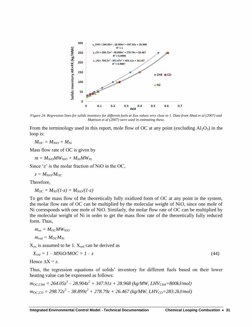
Figure 21 shows the excellent fit offered by a 3rd
order polynomial equation for all the three
fuels. These equations, applicable only when Xox is very close to 1, are used for estimation of
solids inventory.
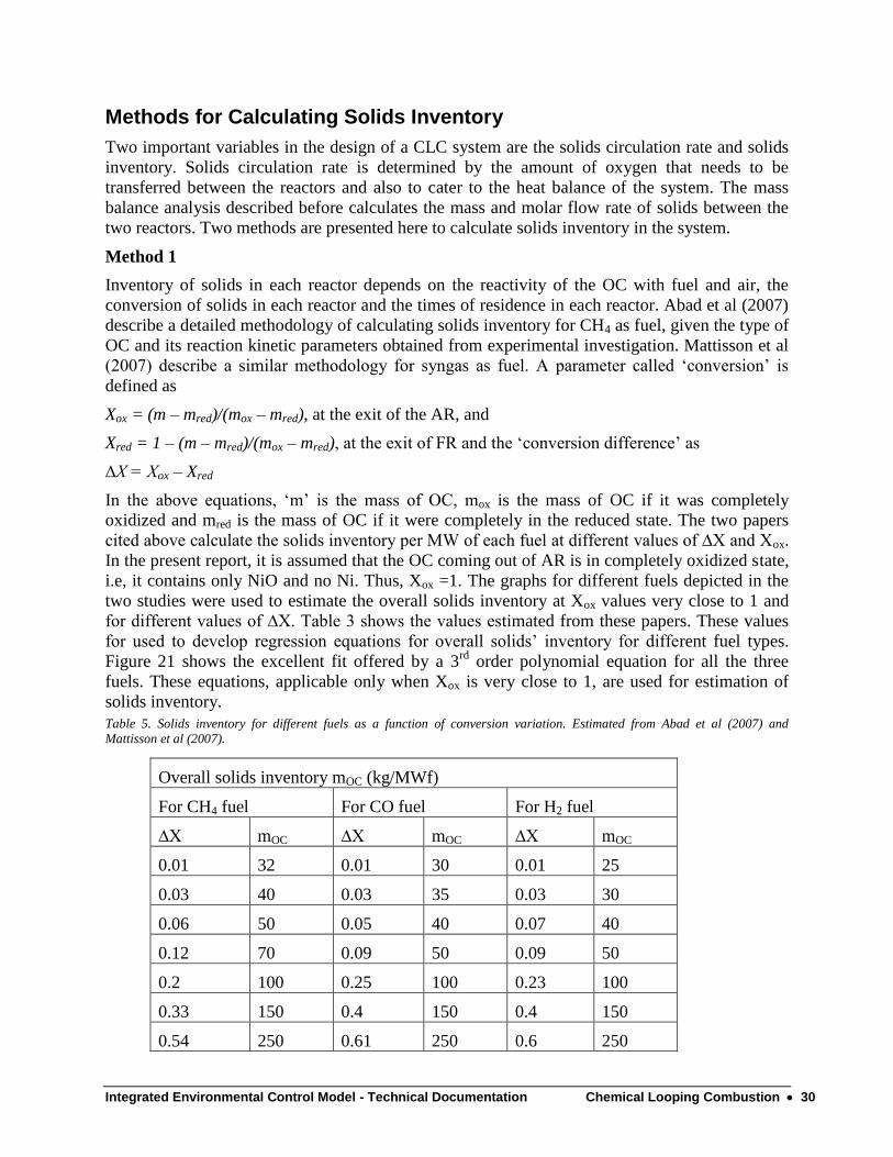
Table 5. Solids inventory for different fuels as a function of conversion variation. Estimated from Abad et al (2007) and
Mattisson et al (2007).
Overall solids inventory mOC (kg/MWf)
For CH4 fuel For CO fuel For H2 fuel
∆X mOC ∆X mOC ∆X mOC
0.01 32 0.01 30 0.01 25
0.03 40 0.03 35 0.03 30
0.06 50 0.05 40 0.07 40
0.12 70 0.09 50 0.09 50
0.2 100 0.25 100 0.23 100
0.33 150 0.4 150 0.4 150
0.54 250 0.61 250 0.6 250
Integrated Environmental Control Model - Technical Documentation Chemical Looping Combustion 31
Figure 24. Regression lines for solids inventory for different fuels at Xox values very close to 1. Data from Abad et al (2007) and
Mattison et al (2007) were used in estimating these.
From the terminology used in this report, mole flow of OC at any point (excluding Al2O3) in the
loop is:
MOC = MNiO + MNi
Mass flow rate of OC is given by
m = MNiOMWNiO + MNiMWNi
Since ‘z’ is the molar fraction of NiO in the OC,
z = MNiO/MOC
Therefore,
MOC = MNi/(1-z) = MNiO/(1-z)
To get the mass flow of the theoretically fully oxidized form of OC at any point in the system,
the molar flow rate of OC can be multiplied by the molecular weight of NiO, since one mole of
Ni corresponds with one mole of NiO. Similarly, the molar flow rate of OC can be multiplied by
the molecular weight of Ni in order to get the mass flow rate of the theoretically fully reduced
form. Thus,
mox = MOCMWNiO
mred = MOCMNi
Xox is assumed to be 1. Xred can be derived as
Xred = 1 – MNiO/MOC = 1 – z (44)
Hence ∆X = z.
Thus, the regression equations of solids’ inventory for different fuels based on their lower
heating value can be expressed as follows:
mOC,CH4 = 264.05z3 – 28.904z
2 + 347.91z + 28.968 (kg/MW, LHVCH4=800kJ/mol)
mOC,CO = 298.72z3 – 38.899z
2 + 278.79z + 26.467 (kg/MW, LHVCO=283.2kJ/mol)
Integrated Environmental Control Model - Technical Documentation Chemical Looping Combustion 32
mOC,H2 = 704.5z3 – 451.67z
2 + 403.12z + 18.147 (kg/MW, LHVH2=241.5kJ/mol)
Overall solids inventory can be expressed as
msolids = (yCH4 mOC,CH4 + yCO mOC,CO + yH2 mOC,H2)LHVfuel (45)
This is the solids inventory for both the reactors combined. Individual solids inventories can be
calculated if the mean residence time of solids in either reactor is known. The solids inventory in
the other reactor can be calculated from the overall solids inventory.
msolids,AR = mOC,in,AR tAR = msolids – msolids,FR (46)
msolids,FR = mOC,in,FR tFR = msolids – msolids,AR (47)
Since this method uses calculations based on figures from published literature, it can prone to
cause errors. Hence, an alternative method is used for inclusion in IECM.
Method 2
Solids inventory can also be calculated if the residence time needed for complete conversion in
each reactor are known. Mean residence time for a NiO/Al2O3 system can be approximated to
be 4s for AR and 60s for FR [Wolf, 2004]. The overall solids inventory can be calculated by
adding equations 46 and 47.
Reactor Design
The most likely design for a CLC system will be comprised of circulating fluidized bed (CFB)
design for AR and FR (Fig 2). For reactor design, the methodology described in Lyngfelt et al
(2001) is used.
The first step is to calculate the area of air reactor, which is a function of the air flow rate
AAR (m2) = Mair,in x 22.4x(TAR+273.15)/(PAR x 273.15 x Ug) (48)
where, PAR is the pressure at which AR operates, Ug is the superficial gas velocity. The most
common value of Ug for these kind of applications is 7m/s, though a range of 5 – 10m/s is
possible [Fan, 2010].
Diameter of vessel D (m) = (4xA/3.14)½.
Maximum diameter of a vessel is 8m [Fan, 2010]. If D > 8m, the air flow is divided in to
multiple vessels.
Pressure drop in the AR is a function of the bed material (solids) and area of AR, which can be
calculated from Eqn 46:
∆pAR (Pa) = msolids,AR x 9.81/AAR (49)
Height of AR is a function of the pressure drop, density of oxygen carrier and void space in the
reactor:
hAR = ∆pAR / (dOC x 9.81 (1 – v)) (50)
where, dOC is the apparent density of solid particles (3446 kg/m3) [Abad et al, 2007].
Integrated Environmental Control Model - Technical Documentation Chemical Looping Combustion 33
Wolf (2004) uses the following equation for solids fraction in the dense bed of AR. Void space
is 1 – solids fraction.
v = 1- ε = -0.053 ln (Ug) + 0.2306
For Ug in the range of 5 – 10 m/s, this value is between 0.11 and 0.15. A value of 0.13 can be
taken as the mean solids fraction in AR.
Volume of the dense bed of AR is calculated as the product of AR height and area
VAR,dense = AAR x hAR (m3)
Volume can also be calculated directly using the equation:
VAR,dense = msolids,AR/(dOC x v) (m3)
This is the volume of dense bed. The overall height of AR riser is about 5 times the height of the
height of dense bed [Wolf, 2004]. Hence the volume of AR can be calculated as;
VAR = 5VAR,dense =5 msolids,AR/(dOC x v) (m3) (51)
Area and height of FR are calculated using similar procedure. For FR with large residence time,
Ug is very low, on the order of 0.05 m/s. From Wolf (2004), the solids fraction in FR (bubbling
bed) can be estimated as:
ε = (Ug/Ut)0.4
,where Ut is the terminal velocity. The typical ratio Ug/Ut is 0.25 and hence solids
fraction (1-v) is about 0.6.
The pressure drop in FR is calculated using this area and the bed material in FR (mOC,FR).
∆pFR (Pa) = msolids,FR x 9.81/AFR (52)
hFR = ∆pFR / (dOC x 9.81 x v)) (53)
VFR = AFR x hFR (m3)
or simply,
VFR = msolids,FR/(dOC x v) (m3) (54)
Integrated Environmental Control Model - Technical Documentation Chemical Looping Combustion 34
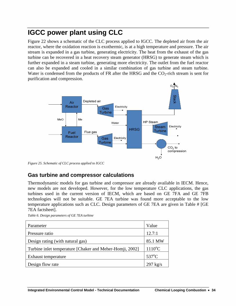
IGCC power plant using CLC Figure 22 shows a schematic of the CLC process applied to IGCC. The depleted air from the air
reactor, where the oxidation reaction is exothermic, is at a high temperature and pressure. The air
stream is expanded in a gas turbine, generating electricity. The heat from the exhaust of the gas
turbine can be recovered in a heat recovery steam generator (HRSG) to generate steam which is
further expanded in a steam turbine, generating more electricity. The outlet from the fuel reactor
can also be expanded and cooled in a similar combination of gas turbine and steam turbine.
Water is condensed from the products of FR after the HRSG and the CO2-rich stream is sent for
purification and compression.
Figure 25. Schematic of CLC process applied to IGCC
Gas turbine and compressor calculations
Thermodynamic models for gas turbine and compressor are already available in IECM. Hence,
new models are not developed. However, for the low temperature CLC applications, the gas
turbines used in the current version of IECM, which are based on GE 7FA and GE 7FB
technologies will not be suitable. GE 7EA turbine was found more acceptable to the low
temperature applications such as CLC. Design parameters of GE 7EA are given in Table # [GE
7EA factsheet].
Table 6. Design parameters of GE 7EA turbine
Parameter Value
Pressure ratio 12.7:1
Design rating (with natural gas) 85.1 MW
Turbine inlet temperature [Chaker and Meher-Homji, 2002] 1110oC
Exhaust temperature 537oC
Design flow rate 297 kg/s
Integrated Environmental Control Model - Technical Documentation Chemical Looping Combustion 35
Using these design parameters, gas turbine and compressor were calibrated using procedures
previously followed in IECM [IGCC tech document]. Gas turbine efficiency is varied to match
the exhaust gas temperature and compressor efficiency is varied to match the overall power
output. Following this calibration procedure, gas turbine and compressor isentropic efficiencies
are fixed at 88.7% and 82.1%, respectively.
It can be noted that in a conventional combined cycle power plant, the flow rate of air that passes
through the compressor is lower than the flow rate of gas passing through the gas turbine. In
contrast, in a CLC system, the amount of air that is compressed is more than the amount that
passes through the gas turbine. Hence, net power output from a CLC system is lower than from a
corresponding conventional gas turbine power plant.
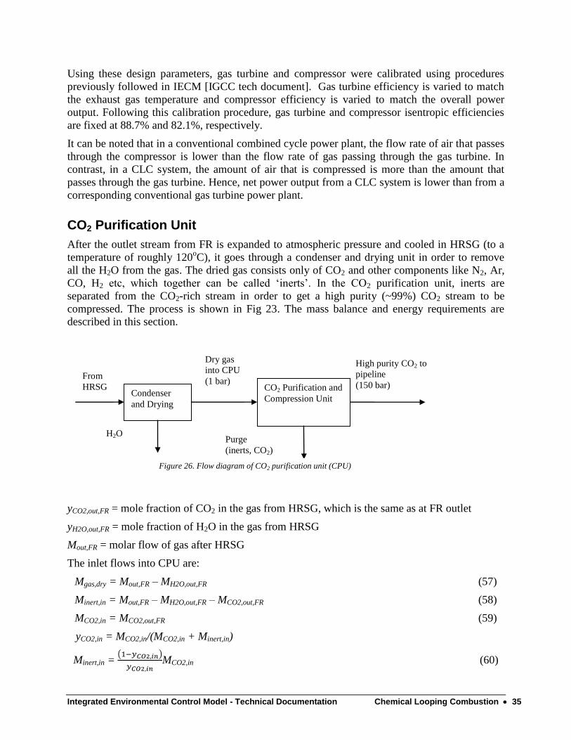
CO2 Purification Unit
After the outlet stream from FR is expanded to atmospheric pressure and cooled in HRSG (to a
temperature of roughly 120oC), it goes through a condenser and drying unit in order to remove
all the H2O from the gas. The dried gas consists only of CO2 and other components like N2, Ar,
CO, H2 etc, which together can be called ‘inerts’. In the CO2 purification unit, inerts are
separated from the CO2-rich stream in order to get a high purity (~99%) CO2 stream to be
compressed. The process is shown in Fig 23. The mass balance and energy requirements are
described in this section.
yCO2,out,FR = mole fraction of CO2 in the gas from HRSG, which is the same as at FR outlet
yH2O,out,FR = mole fraction of H2O in the gas from HRSG
Mout,FR = molar flow of gas after HRSG
The inlet flows into CPU are:
Mgas,dry = Mout,FR – MH2O,out,FR (57)
Minert,in = Mout,FR – MH2O,out,FR – MCO2,out,FR (58)
MCO2,in = MCO2,out,FR (59)
yCO2,in = MCO2,in/(MCO2,in + Minert,in)
Minert,in =
MCO2,in (60)
Condenser
and Drying
CO2 Purification and
Compression Unit
From
HRSG
Dry gas
into CPU
(1 bar)
High purity CO2 to
pipeline
(150 bar)
H2O Purge
(inerts, CO2)
Figure 26. Flow diagram of CO2 purification unit (CPU)
Integrated Environmental Control Model - Technical Documentation Chemical Looping Combustion 36
Assume the molar ratio of CO2 and inerts in the purge gas is ‘a’. This value is determined by
thermodynamic calculations and is not available at this point of time. So, this needs to be
assumed from empirical data.
a = MCO2,purge/Minert,purge
Purity of CO2 in the stream to pipeline is given by
yCO2,out = MCO2,out/(MCO2,out + Minert,out)
Minert,in = Minert,out + Minert,purge
Minert,in = Minert,out + MCO2,purge/a
= Minert,out + (MCO2,in – MCO2,out)/a
This can be rearranged in terms of mole fraction of CO2:
or
(61)
If ‘a’ is known and yCO2,out is fixed, MCO2,out can be calculated.
Mass of CO2 captured is given by
mCO2,captured = 44MCO2,out
(62)
Efficiency of capture is given by:
ηCO2,capture = MCO2,out / MCO2,in =
(63)
For energy requirements, the estimation given in Aspelund and Jordal (2007) is used. Figure 24
shows a result from that paper, from which line P2 is applicable to CLC purpose. The figure
shows energy requirement to clean and compress flue gas from 1 bar to 150 bar, as a function of
the amount of inert material (in the form of Nitrogen). The mole fraction of inerts is 1 – mole
fraction of CO2.
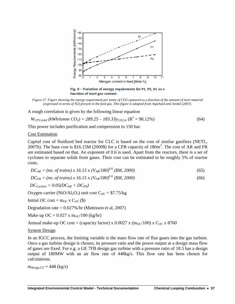
Integrated Environmental Control Model - Technical Documentation Chemical Looping Combustion 37
Figure 27. Figure showing the energy requirement per tonne of CO2 cpatured as a function of the amount of inert material
(expressed in terms of N2) present in the feed gas. This figure is adopted from Aspelund and Jordal (2007).
A rough correlation is given by the following linear equation
WCPU,total (kWh/tonne CO2) = 289.25 – 183.33yCO2,in (R2 = 98.12%) (64)
This power includes purification and compression to 150 bar.
Cost Estimation
Capital cost of fluidized bed reactor for CLC is based on the cost of similar gasifiers (NETL,
2007b). The base cost is $16.15M (2000$) for a CFB capacity of 180m3. The cost of AR and FR
are estimated based on that. An exponent of 0.6 is used. Apart from the reactors, there is a set of
cyclones to separate solids from gases. Their cost can be estimated to be roughly 5% of reactor
costs.
DCAR = (no. of trains) x 16.15 x (VAR/180)0.6
($M, 2000) (65)
DCFR = (no. of trains) x 16.15 x (VFR/180)0.6
($M, 2000) (66)
DCCyclone = 0.05(DCAR + DCFR)
Oxygen carrier (NiO/Al2O3) unit cost COC = $7.75/kg
Initial OC cost = mOC x COC ($)
Degradation rate = 0.027%/hr (Mattisson et al, 2007)
Make up OC = 0.027 x mOC/100 (kg/hr)
Annual make-up OC cost = (capacity factor) x 0.0027 x (mOC/100) x COC x 8760
System Design
In an IGCC process, the limiting variable is the mass flow rate of flue gases into the gas turbine.
Once a gas turbine design is chosen, its pressure ratio and the power output at a design mass flow
of gases are fixed. For e.g. a GE 7FB design gas turbine with a pressure ratio of 18.5 has a design
output of 180MW with an air flow rate of 448kg/s. This flow rate has been chosen for
calculations.
mdesign,GT = 448 (kg/s)
Integrated Environmental Control Model - Technical Documentation Chemical Looping Combustion 38
Mdesign,GT = mdesign,GT/29 (kmol/s)
The air flow into the air reactor of the CLC system should be such that the outlet flow should be
equal to the design value of the gas turbine.
From Eqn 18, MO2,out = MO2,in – 0.5MNi,in
Mair,out = MO2,out + MN2,out = MO2,in – 0.5MNi,in + MN2,in = Mair,in – 0.5MNi,in
The Ni coming into AR is equal to the stoichiometric amount with respect to the fuel. The flow
rate of air at the outlet of AR should be equal to the design flow rate. Therefore,
Mair,in = Mdesign,GT + 0.5MNiO,stoic = Mdesign,GT + 0.5sNiO,fMfuel
(67)
For NiO, stoichiometric ratio with respect to fuel is half of the stoichiometric ratio of O2 in air
with respect to fuel. Thus,
Mair,in = Mdesign,GT + sO2,fMfuel (68)
The actual air can be expressed in terms of stoichiometric air and excess air ratio, as in Eqn 69.
(1+x)Mair,stoic = Mdesign,GT + sO2,fMfuel (69)
Stoichiometric air can be expressed in terms of fuel flow and stoichiometric ratio of O2 with
respect to fuel. One mole of O2 is equivalent to 4.76 moles of air.
(1+x)(4.76 sO2,f)Mfuel = Mdesign,GT + sO2,fMfuel
From the above equation, fuel flow requirement of the CLC system can be calculated for a
choice of gas turbine.
(70)
Once the required fuel flow is known, required air flow at the inlet to AR can be calculated from
Eqn 68.
Calculation procedure
The calculation procedure for the CLC system can be listed as follows:
1. Choose the gas turbine. This fixes the operating pressure (PAR), design air flow
(Mdesign,GT) and the turbine output power. This also fixes the pressure ratio of the
compressor and hence the temperature of air (Tair) going into AR, which is calculated
using the compressor model equations.
2. Fuel composition is fixed by the choice of gasifier. From the fuel composition, calculate
the stoichiometric O2 (sO2,f)and NiO (sNiO,f) ratios. Fuel temperature is fixed at 50oC
because it comes from the sulfur cleanup process which operates at 50oC.
3. Choose the air reactor temperature (TAR). Usual operating temperatures using an NiO-
based OC range from 900 – 1200 oC.
4. Choose the excess NiO ratio (z)
5. Since TAR and z are fixed, fuel reactor temperature (TFR) can be calculated from the
regression Eqns 41 – 43, depending on the type of gasifier
Integrated Environmental Control Model - Technical Documentation Chemical Looping Combustion 39
6. The OC temperature (TMeO) going into the AR is the same as TFR.
7. Since TMeO, Tair, TAR and z are known, excess air ratio (x) can be calculated from Eqn 22.
This denotes the excess air required to maintain the air reactor temperature.
8. Flow rate of fuel (Mfuel) can be calculated since Mdesign,GT and x are known.
9. FR calculations - based on fuel flow rate and composition, flow rates of individual
components can be obtained. Based on the thermodynamic model for FR described
before, the flow rates of different components, including solids and gases, at the outlet of
FR can be calculated.
10. AR calculations – based on the fuel flow rate and excess air ratio, inlet air flow can be
calculated. Based on the thermodynamic model for AR described before, the flow rates of
different components, including solids and gases, at the outlet of AR can be calculated.
11. Overall solids inventory can be calculated based on z and Eqn 45. Assuming a residence
time of solids in the FR which is typically around 60s [Wolf, 2010], the solids inventory
in the FR can be calculated using Eqn 46 and hence solids inventory in the AR
12. Based on the calculations above, reactor dimensions can be estimated using the procedure
described in the reactor design section
13. From the reactor volume, capital cost can be estimated using eqn#. O&M costs can be
calculated based on the solids flow rates.
14. Energy output from the gas turbine and expander and energy required for compressor can
also be calculated
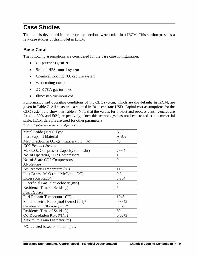
Integrated Environmental Control Model - Technical Documentation Chemical Looping Combustion 40
Case Studies The models developed in the preceding sections were coded into IECM. This section presents a
few case studies of this model in IECM.
Base Case
The following assumptions are considered for the base case configuration:
GE (quench) gasifier
Selexol H2S control system
Chemical looping CO2 capture system
Wet cooling tower
2 GE 7EA gas turbines
Illinois# bituminous coal
Performance and operating conditions of the CLC system, which are the defaults in IECM, are
given in Table 7. All costs are calculated in 2011 constant USD. Capital cost assumptions for the
CLC system are shown in Table 8. Note that the values for project and process contingencies are
fixed at 30% and 50%, respectively, since this technology has not been tested at a commercial
scale. IECM defaults are used for other parameters.
Table 7. Input assumptions in IECM for base case
Metal Oxide (MeO) Type NiO
Inert Support Material Al2O3
MeO Fraction in Oxygen Carrier (OC) (%) 40
CO2 Product Stream
Max CO2 Compressor Capacity (tonne/hr) 299.4
No. of Operating CO2 Compressors 1
No. of Spare CO2 Compressors 0
Air Reactor
Air Reactor Temperature (oC) 1100
Inlet Excess MeO (mol MeO/mol OC) 0.3
Excess Air Ratio* 3.204
Superficial Gas Inlet Velocity (m/s) 7
Residence Time of Solids (s) 5
Fuel Reactor
Fuel Reactor Temperature (oC) 1045
Stoichiometric Ratio (mol O2/mol fuel)* 0.3842
Combustion Efficiency (%)* 99.22
Residence Time of Solids (s) 60
OC Degradation Rate (%/hr) 0.0272
Maximum Train Diameter (m) 8
*Calculated based on other inputs
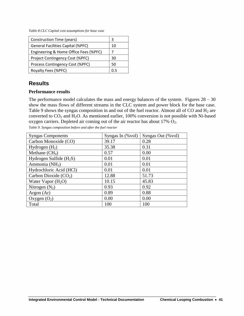
Integrated Environmental Control Model - Technical Documentation Chemical Looping Combustion 41
Table 8.CLC Capital cost assumptions for base case
Construction Time (years) 3
General Facilities Capital (%PFC) 10
Engineering & Home Office Fees (%PFC) 7
Project Contingency Cost (%PFC) 30
Process Contingency Cost (%PFC) 50
Royalty Fees (%PFC) 0.5
Results
Performance results
The performance model calculates the mass and energy balances of the system. Figures 28 – 30
show the mass flows of different streams in the CLC system and power block for the base case.
Table 9 shows the syngas composition in and out of the fuel reactor. Almost all of CO and H2 are
converted to CO2 and H2O. As mentioned earlier, 100% conversion is not possible with Ni-based
oxygen carriers. Depleted air coming out of the air reactor has about 17% O2.
Table 9. Syngas composition before and after the fuel reactor
Syngas Components Syngas In (%vol) Syngas Out (%vol)
Carbon Monoxide (CO) 39.17 0.28
Hydrogen (H2) 35.38 0.31
Methane (CH4) 0.57 0.00
Hydrogen Sulfide (H2S) 0.01 0.01
Ammonia (NH3) 0.01 0.01
Hydrochloric Acid (HCl) 0.01 0.01
Carbon Dioxide (CO2) 12.88 51.73
Water Vapor (H2O) 10.15 45.83
Nitrogen (N2) 0.93 0.92
Argon (Ar) 0.89 0.88
Oxygen (O2) 0.00 0.00
Total 100 100
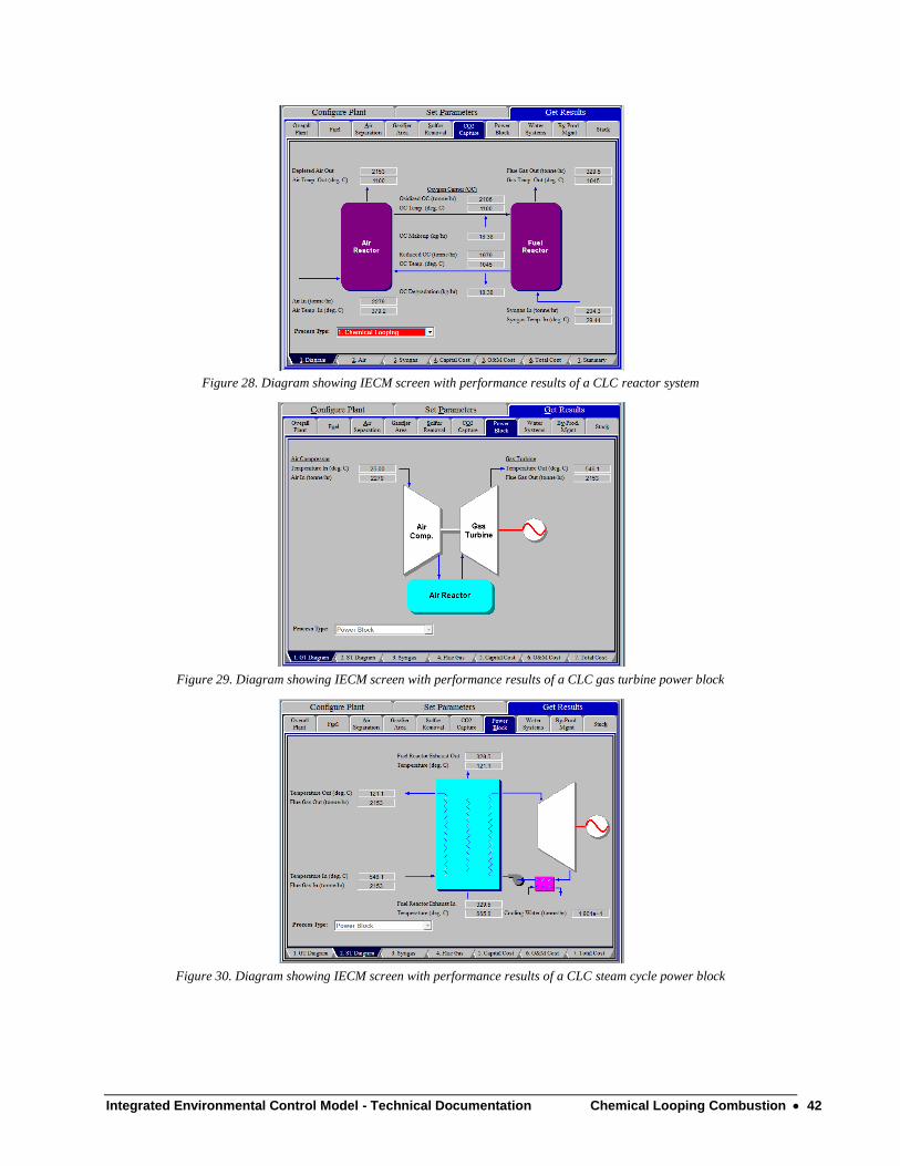
Integrated Environmental Control Model - Technical Documentation Chemical Looping Combustion 42
Figure 28. Diagram showing IECM screen with performance results of a CLC reactor system
Figure 29. Diagram showing IECM screen with performance results of a CLC gas turbine power block
Figure 30. Diagram showing IECM screen with performance results of a CLC steam cycle power block
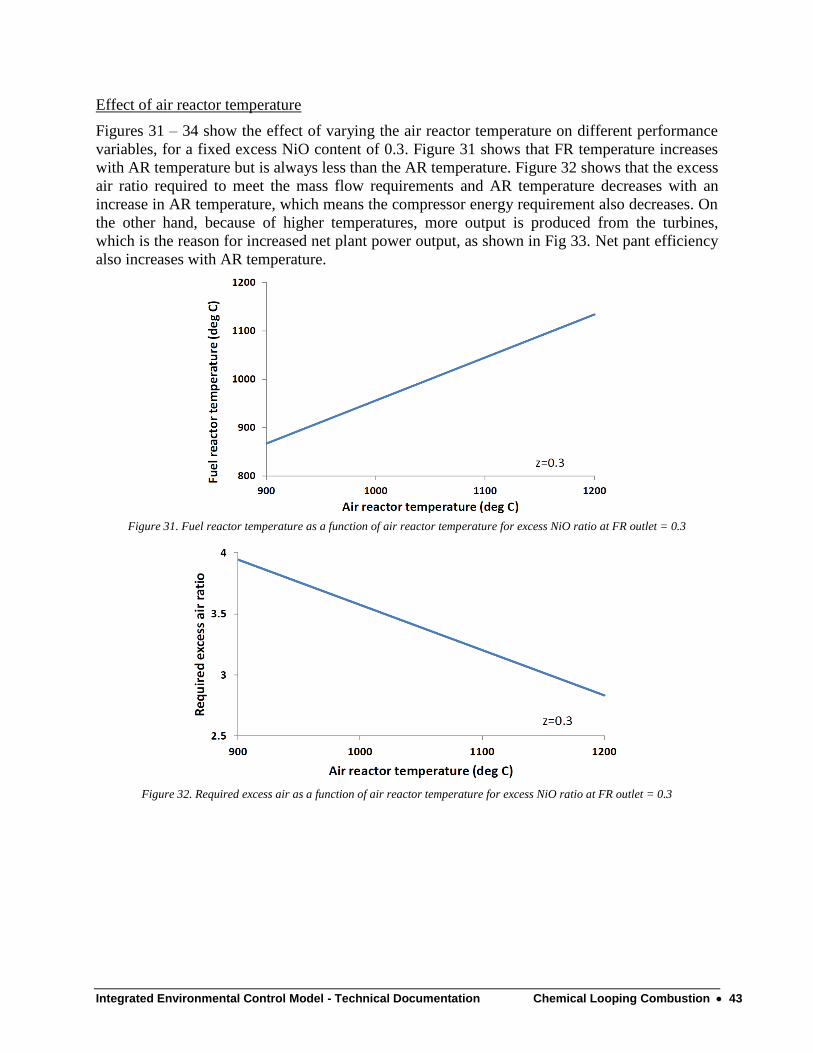
Integrated Environmental Control Model - Technical Documentation Chemical Looping Combustion 43
Effect of air reactor temperature
Figures 31 – 34 show the effect of varying the air reactor temperature on different performance
variables, for a fixed excess NiO content of 0.3. Figure 31 shows that FR temperature increases
with AR temperature but is always less than the AR temperature. Figure 32 shows that the excess
air ratio required to meet the mass flow requirements and AR temperature decreases with an
increase in AR temperature, which means the compressor energy requirement also decreases. On
the other hand, because of higher temperatures, more output is produced from the turbines,
which is the reason for increased net plant power output, as shown in Fig 33. Net pant efficiency
also increases with AR temperature.
Figure 31. Fuel reactor temperature as a function of air reactor temperature for excess NiO ratio at FR outlet = 0.3
Figure 32. Required excess air as a function of air reactor temperature for excess NiO ratio at FR outlet = 0.3
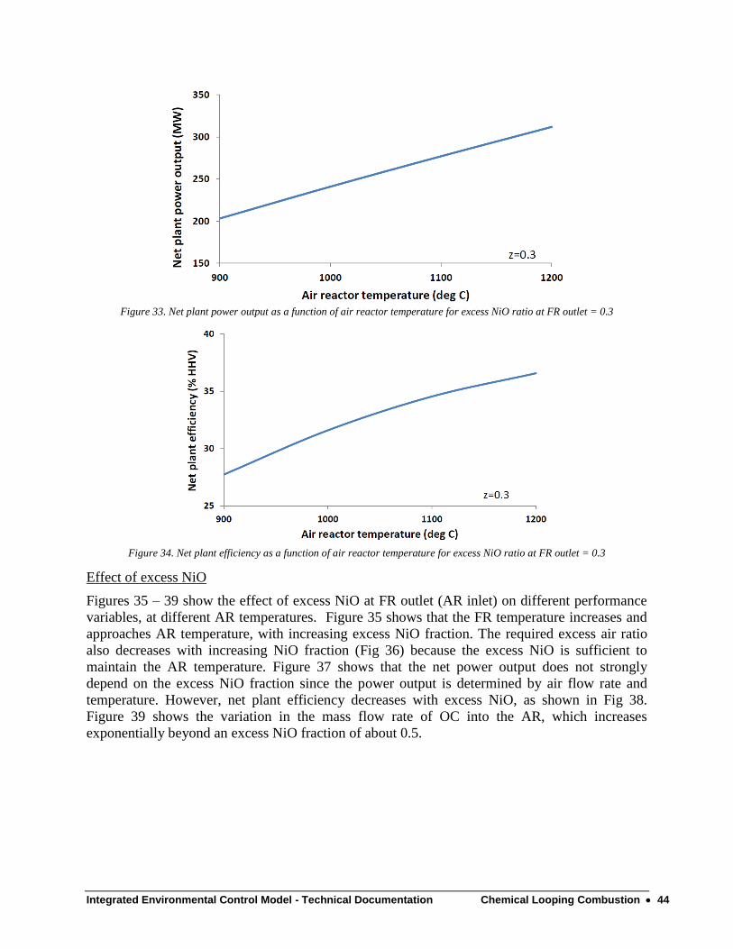
Integrated Environmental Control Model - Technical Documentation Chemical Looping Combustion 44
Figure 33. Net plant power output as a function of air reactor temperature for excess NiO ratio at FR outlet = 0.3
Figure 34. Net plant efficiency as a function of air reactor temperature for excess NiO ratio at FR outlet = 0.3
Effect of excess NiO
Figures 35 – 39 show the effect of excess NiO at FR outlet (AR inlet) on different performance
variables, at different AR temperatures. Figure 35 shows that the FR temperature increases and
approaches AR temperature, with increasing excess NiO fraction. The required excess air ratio
also decreases with increasing NiO fraction (Fig 36) because the excess NiO is sufficient to
maintain the AR temperature. Figure 37 shows that the net power output does not strongly
depend on the excess NiO fraction since the power output is determined by air flow rate and
temperature. However, net plant efficiency decreases with excess NiO, as shown in Fig 38.
Figure 39 shows the variation in the mass flow rate of OC into the AR, which increases
exponentially beyond an excess NiO fraction of about 0.5.
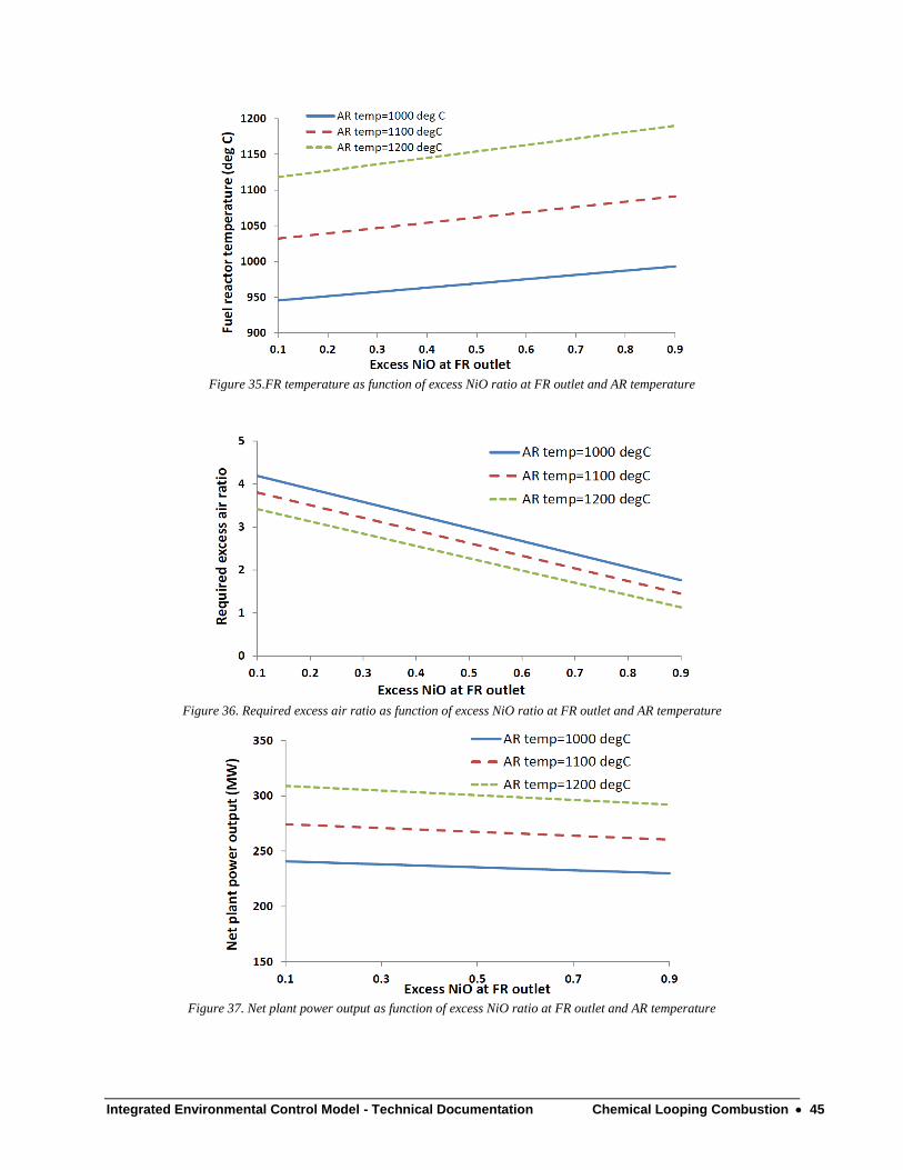
Integrated Environmental Control Model - Technical Documentation Chemical Looping Combustion 45
Figure 35.FR temperature as function of excess NiO ratio at FR outlet and AR temperature
Figure 36. Required excess air ratio as function of excess NiO ratio at FR outlet and AR temperature
Figure 37. Net plant power output as function of excess NiO ratio at FR outlet and AR temperature
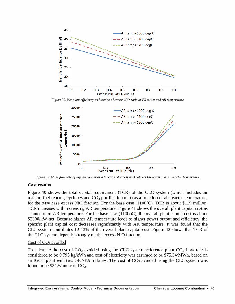
Integrated Environmental Control Model - Technical Documentation Chemical Looping Combustion 46
Figure 38. Net plant efficiency as function of excess NiO ratio at FR outlet and AR temperature
Figure 39. Mass flow rate of oxygen carrier as a function of excess NiO ratio at FR outlet and air reactor temperature
Cost results
Figure 40 shows the total capital requirement (TCR) of the CLC system (which includes air
reactor, fuel reactor, cyclones and CO2 purification unit) as a function of air reactor temperature,
for the base case excess NiO fraction. For the base case (1100oC), TCR is about $119 million.
TCR increases with increasing AR temperature. Figure 41 shows the overall plant capital cost as
a function of AR temperature. For the base case (1100oC), the overall plant capital cost is about
$3300/kW-net. Because higher AR temperature leads to higher power output and efficiency, the
specific plant capital cost decreases significantly with AR temperature. It was found that the
CLC system contributes 12-13% of the overall plant capital cost. Figure 42 shows that TCR of
the CLC system depends strongly on the excess NiO fraction.
Cost of CO2 avoided
To calculate the cost of CO2 avoided using the CLC system, reference plant CO2 flow rate is
considered to be 0.795 kg/kWh and cost of electricity was assumed to be $75.34/MWh, based on
an IGCC plant with two GE 7FA turbines. The cost of CO2 avoided using the CLC system was
found to be $34.5/tonne of CO2.
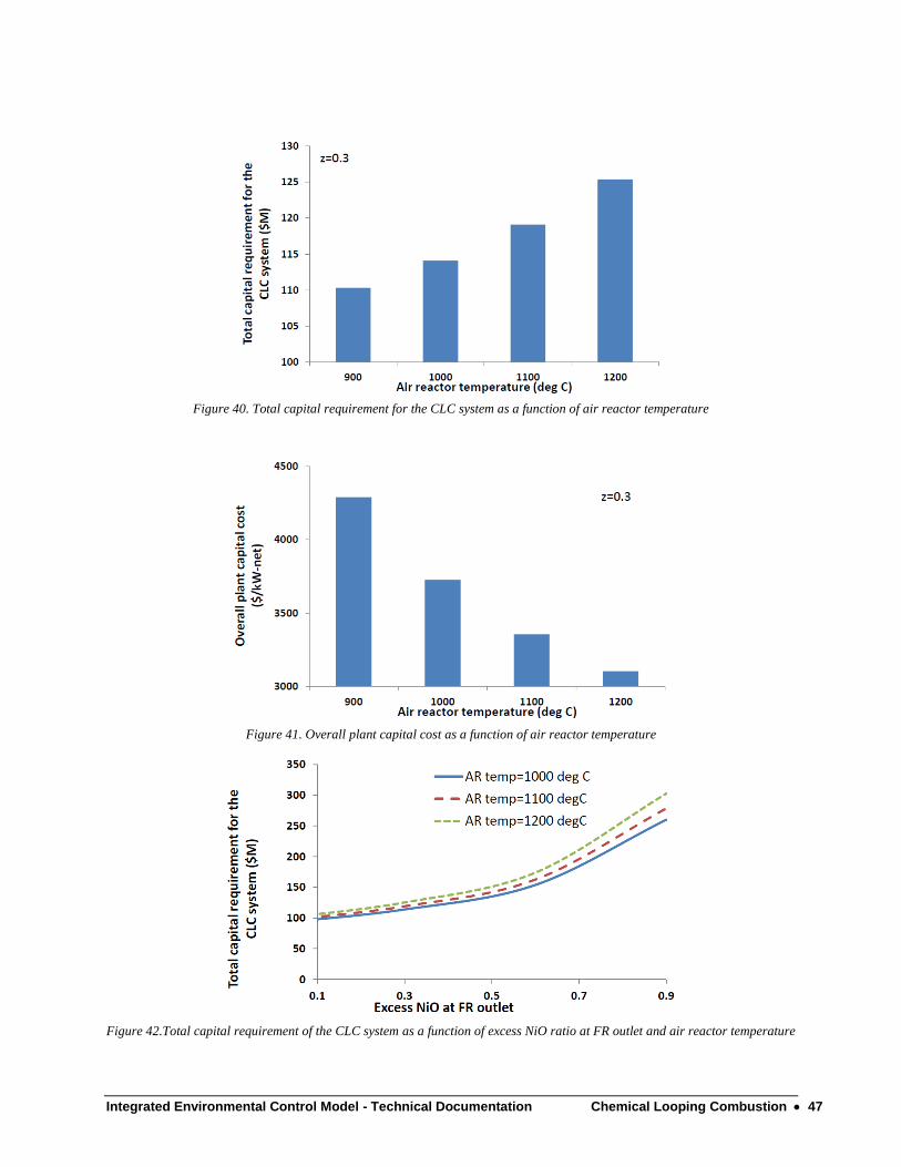
Integrated Environmental Control Model - Technical Documentation Chemical Looping Combustion 47
Figure 40. Total capital requirement for the CLC system as a function of air reactor temperature
Figure 41. Overall plant capital cost as a function of air reactor temperature
Figure 42.Total capital requirement of the CLC system as a function of excess NiO ratio at FR outlet and air reactor temperature
Integrated Environmental Control Model - Technical Documentation Chemical Looping Combustion 48
Comparison with other configurations
In the current version of IECM, a base plant without CCS using GE 7EA turbine technology
does not exist. Hence, a direct comparison of the plant with CCS (using CLC) to a plant without
CCS is not possible. However, the user may change the design parameters (pressure ratio,
temperature, isentropic efficiency) for a plant using GE 7FA/7FB turbine technologies to match
the output with a 7EA turbine, in order to get a sense of the additional performance and cost
penalties of CCS with CLC.
To compare the CLC system with a Selexol process, the IECM user should adjust the number of
turbines so that the amount of CO2 captured in both the plants is comparable.
Conclusion
Thermodynamic and cost models were developed for pre-combustion CO2 capture using
chemical looping combustion technology, and implemented into IECM. The use of IECM to
estimate the performance and cost of an IGCC power plant with CLC-based CO2 capture was
also demonstrated in this report.
References
Abad A., Adanez J., Garcia-Labiano F., de Diego L.F., Gayan P., and Ceyala J., 2007, “Mapping
the range of operational conditions for Cu-, Fe-, and Ni-based oxygen carriers in chemical-
looping combustion”, Chemical Engineering Science, 62, 533 – 549.
Abdulally I. et al, 2010, “Alstom’s chemical looping combustion coal power technology
development prototype”, 1st Intl. Chemical Looping Conference, 17
th – 19
th March, Lyon,
France.
Alanso M., Rodriguez N., Gonzalez B., Grasa G., Murillo R., and Abanades J.C., 2010, “CO2
capture from combustion flue gases with a calcium oxide chemical loop”, Intl. Journal of
Greenhouse Gas Control, Special Issue, 4, 2, 167 – 173.
Andrus H., 2009, “Chemical looping combustion coal power technology development
prototype”, CO2 Capture Technology Conference, US DOE/NETL, 24th
– 26th
March,
Pittsburgh, USA.
Andrus H.E., Chiu J.H., Thibeault P.R., and Brautsch A., 2009, “Alstom’s calcium oxide
chemical looping combustion coal power technology development”, The 34th
Intl. Technical
Conference on Clean Coal & Fuel Systems, May 31st – June 4
th, Clearwater, FL, USA.
Aspelund A., and Jordal K., 2007, “Gas conditioning – the interface between CO2 capture and
transport,” Intl. Journal of Greenhouse Gas Control, 1, 342 – 354.
Blamey J., Anthony E.J., Wang J., and Fennell P.S., 2010, “The calcium looping cycle for large-
scale CO2 capture”, Progress in Energy and Combustion Science, 36, 260 – 279.
Brandvoll O. and Bolland O., 2004, “Inherent CO2 capture using chemical looping combustion
in a natural gas fired power cycle”, Transaction of ASME, 126, 316 – 321, April.
Fan L.S., 2010, “Chemical looping processes”, 1st Intl. Conference on Chemical Looping, 17
th –
19th
March, Lyon, France.
Integrated Environmental Control Model - Technical Documentation Chemical Looping Combustion 49
Fan L.S., “Chemical looping systems for fossil energy conversions”, AIChE and John Wiley &
Sons, Inc. New Jersey, 2010.
Fang H., Haibin L, and Zengli Z., 2009, “Advancements in development of chemical-looping
combustion: a review”, Review article, Intl. Journal of Chemical Engineering.
Ishida M., and Jin H., 1994, “A new advanced power-generation system using chemical-looping
combustion”, Energy, 4, 415 – 422.
Jerndal E., Mattisson T., and Lyngfelt A., 2006, “Thermal analysis of chemical-looping
combustion”, Chemical Engineering Research and Design, 84 (A9), 795 – 806.
Hossain M.M and de Lasa H., 2008, “Chemical-looping combustion (CLC) for inherent CO2
separations – a review”, Chemical Engineering Science, 63, 4433 – 4451.
Kolbitsch P., Proll T., and Hofbauer H., 2009, “Modeling of a 120 kW chemical looping
combustion reactor system using a Ni-based oxygen carrier”, Chemical Engineering Science,
64, 99 – 108.
Kolbitsch P. et al, 2010, “Operating experience with chemical looping combustion in a 120 kW
dual circulating fluidized bed (DCFB) unit”, Intl. Journal of Greenhouse Gas Control, 4, 180
– 185.
Lyngefelt A., Leckner B. and Mattisson T., 2001, “A fluidized-bed combustion process with
inherent CO2 separation; application of chemical-lopping combustion”, Chemical
Engineering Science, 56, 3101 – 3113.
Lyngfelt A., “Oxygen carriers for chemical looping combustion – operational experience”, 1st
Intl. Chemical Looping Conference, 17th
– 19th
March, Lyon, France.
Mattisson T., Lyngfelt A. and Leion H., 2009, “Chemical looping with oxygen uncoupling for
combustion of solid fuels”, Intl. Journal of Greenhouse Gas Control, 3, 1, 11 – 19.
Mattisson T., Garcia-Labiano F., Kronberger B., Lyngfelt A., Adanez J., and Hofbauer H., 2007,
“Chemical-looping combustion using syngas as fuel”, Intl. Journal of Greenhouse Gas
Control, 1, 158 – 169.
NETL, 2007a, “Cost and performance baseline for fossil energy plants”, NETL/DoE-2007/1281,
May
NETL, 2007b, Chemical-looping process in a coal-to-liquids configuration, DOE/NETL-
2008/1307.
Rizeq et al., 2003, “Fuel-flexible gasification-combustion technology for production of hydrogen
and sequestration-ready carbon dioxide”, Report to US DoE/NETL, DE-FC26-00FT40974.
Smith J. M, Van Ness H. C, Abbott M. M, “Introduction to chemical engineering
thermodynamics”, 7th
ed, McGraw Hill publication, New York, 2005.


![Alstom’s [GE] Chemical Looping Combustion Technology ......Imagination at work Alstom’s [GE] Chemical Looping Combustion Technology with CO2 Capture for New and Existing Coal-fired](https://img.pdfslide.us/doc/110x75/60fbc9baac9da0424a530e18/alstomas-ge-chemical-looping-combustion-technology-imagination-at-work.jpg)