Embed Size (px)
Citation preview

1'-'
Ie:2qA #~(, 'CIVIL ENGINEERING STUDIES
:STRUCTURAL RESEARCH SERIES NO. 261
INTERACTION OF PLANE ELASTIC WAVES
ITH AN ELASTIC CYLINDRICAL SHELL
By T. YOSHIHARA
A. R. ROBINSON
and
J. l. MERRITT
A Technical Report
of a Research Program
Sponsored by
THE~ OFFICE OF NAVAL. RESEARCH
DEPARTMENT OF THE NAVY
Contract Nonr 1 834(03)
Project NR-064-1 83
UNIVERSITY OF ILLINOIS
URBANA, ILLINOIS
JANUARY 1963

INTERACTION OF PLANE ELASTIC WAVES
WITH AN ELASTIC CYLINDRICAL SHELL
By
T. Yoshihara
A. R. Robinson
and
J. L. Merritt
A Technical Report of a Research Program
Sponsored by
THE OFFICE OF NAVAL RESEARCH DEPARTMENT OF THE NAVY Contract Nonr 1834(03)
Project NR-064-183
UNIVERSITY OF ILLINOIS
URBANA, ILLINOIS
JANUARY 1963

ABSTRACT
The purpose of this study was to investigate the interaction of plane
elastic waves with a thinJ hollow; cylindrical shell embedded in an elastic
medium 0
The cylindrical shell is considered to be elastic, isotropic J homo
geneous, and of infinite lengtho It is surrounded by an elastic, isotropic,
and homogeneous medium whose motions conform to the ordinary theory of elas
ticityo A plane stress wave, either dilatational or shear, with a step varia
tion in time, whose wave front travels in a direction perpendicular to the
cylinder axis, envelops the sheIla Later J a Duhamel integral is used to study
other wave shapes for the incident stress o
The response of the shell is studied by expressing the two components
of displacement, radial and tangential, in terms of Fourier series, each term
of which is called a modeo The equations of motion of the shell in vacuo
are derived from expressions giving the strain and kinetic energies due to
generalized external forceso Forces on the shell result from the stresses in
the medium at the boundary 0 Stresses in the medium are taken to be the sum
of the stresses due to the incoming stress wave expressed in terms of Fourier
series whose coefficients are known; and those due to the reflected and dif
fracted effects expressed in terms of a pair of displacement potentials rep
resenting waves diverging from the axis of the shello
The equations to be solved consist of two pairs of coupled integro
differential equations in the generalized coordinates of the shell and the
displacement potentialso By use of a digital computer they are solved mode
wise by a step-by-step iterative integration technique known as the Newmark
Beta Method, with which values for the potential functions, and the acceler-
ations y velocities, and displacements of the shell are determinedo Stresses
in the shell are £o~~d from the displacements, and the values of the potential
functions permit determination of stresses for any point in the mediumo
Although the equations are written to include an infinite number
of modes, only the first three modes are considered in detailo The computed
solution is compared with values obtained from a series expansion of the
equations, which is valid for short times J and with the static solution based
on the theory of elasticity to which the general solution should approach
asymptoticallyo In addition, the results of two particular problems are
compared with results given in another studyo
Numerical solutions are obtained to determine the effect of the
several parameters which describe the relative physical properties of the
shell and meditimo Results are presented in tabular and graphical forma

ACKNOWLEDGMENT
The study reported herein was conducted under a program sponsored
by the United states Navy Bureau of Yards and Docks and administered by the
Superintendent, U. S. Naval Postgraduate School 0 The report is based upon
a thesis prepared by T. Yoshihara in partial fulfillment of the requirements
for the degree of Doctor of Philosophy in Ci vi.l Engineering.
The report ~las prepared under the general direction of Dr 0 NoM.
Ne\vmark, Head, Department of Civil Engineeringo The assistance of Dr ~ SoL 0
Paul, Instructor in Civil Engineering, is gratefully acknowledgecL
Appreciation is also expressed to the personnel of the University
of Illinois Digital Computer Laboratory for their cooperation.

II.
TABLE OF CONTENTS
INTRODUCTION . . . . . . .
1.1 1.2 1·3 1.4 1·5 1.6
General Remarks . . . . . Statement of Problem. . Basic Assumptions . . Method of Approach. . . ·Previous Work. Notation ..... .
BASIC EQUATIONS .
2.1
2.2
2·3 2.4 2·5
E~uations for the Medium. 2.11 Dilatational Wave 2.12 Shear Wave ..... E~uations for the Shell . 2.21 Dilatational Wave . 2.22 Shear Wave .... 2.23 Effect of Additional Mass . Boundary Conditions . . . . . . . . . . Summary of E~uations in Non~Dimensionalized Form. . OtherE~uations of Interest . . . . . . . . . . . .
III. METHOD OF SOLUTION .
IV.
3·1 3·2 3·3 3·4 3·5 3.6 3·7
General . ~ . . Numerical Integration of the Potential Functions .. Solution of the Basic E~uations . Stresses of the Shell and Medium. . Time Dependent Stress Wave ..... . Description of the Computer Program . Short-Time Approximation. . . . ..
DISCUSSION OF RESULTS. . ...... .
4.1 General. . . . . . ..... . 4.2 Modal Response of Shell and Medium .. 4.3 Short-Time and Asymptotic Comparison ..... . 4.4 Effect of Parameters ...... . 4.5 Response to Time Varying Incident Wave .. 4.6 Comparison with Previous Work. 4.7 Conclusions .......... .
BIBLIOGRAPHY . . . . .
iv
Page
1
1 1 2 3 4 5
9
9 12 18 21 23 25 26 28 29 32
34
34 34 40 43 46 46 48
53 5.) 54 56 59 61 61 62
64

APPENDIX A.
APPENDIX B.
TABLE OF CONTENTS (Cont'd)
DERIVATION OF THE EXPRESSIONS INVOLVING THE POfJ;ENTIAL FUNCTIONS . . . . . 0 • • • • 0 • 0 • • • •
A.l A.2 A·3
General Form of the Potential Function . Velocity Terms ...... . Stre s sTerms . . . . . . . . . . . . . .
STATIC SOLUTION .
Bol Dilatational Wave. Boll n = 0 Mode .. B.12 n = 2 Mode .
B.2 Shear Wave ...
v
Page
65
65 68 69
71 71 72 74 76
101 General Remarks
CHAPTER I
INTRODUCTION
The problem of designing underground protective structures to
1
resist the effects of nuclear weapons has become increasingly important in
recent years with the development of modern weapons whose destructi.ve capacity
is overwhelming. Engineers in thi.s fi.eld are hampered to a great extent by a
lack of theoretical information on how structures i.n media such as soil or
rock behave when subjected to dynami.c loads. Even for static loads alone)
much of the design practice today is of a semi-empirical nature.
When a nuclear explosion occurs) stress waves are transmitted
through the air and ground. How are they transmitted and how are they modifi.ed
by the presence of a structure embedded i.n the medium? How does the structure
respond?
The purpose of this report is to st'udy one aspect of the problem)
the interaction between the medium and structure.
1.2 Statement of Problem
The problem considered here consi.sts of analyzing the elastic
response of a hollow cylindrical shell em~bedded in an elasti.c
medium when subjected to an incident plane stress wave traveling in a direction
perpendicular to the axis of the shell 0 Some questions with which thi,s problem
may be associated are ~ Do tunnel li.nings in contact with rock afford a measure
of protection significantly higher than an unlined opening? lfua t magnitude
and time variation of displacement ) velocity) and accelera ti.on would equipment
mounted within such a structure be subjected to? How are stress waves within

the medi.um modified in the vicinity of the shel17 This study was conducted
in an attempt to find some qualitati.ve and quantitative answers to these
questions within the limitations imposed by the assumptions noted below.
103 Basi.c Assumptions
2
The cylindrical shell is considered to be of infinite length, and
is embedd,ed in an elastic medium of infinite extent in all directions. A
plane stres s wave whose front travels in a directi,on perpendicular to the
cylinder axis envelops the shell, Strai,ns parallel to the axis in both the
medium and shell are as sumed to vanish; thus.j since each cros s section of the
shell is exactly similar to every other, the problem is reduced to one of
plane strai,no
In the mathematical development of the problem certai,n basic
assumpti.ons 'were made, the most important of which are given here with a few
explanatory remark.s~
(1) The medium is consi.dered to be homogeneous, isotropic, and
linearly elastic. This implies that the ordinary theory of stress wave
propagati,on applies 0 In view of the non-homogeneous, non-isotropi,c, and
non-elastic characteristics of most materials encountered in nature, this
is a severe limi,tation; however, current theories of stress propagation
through such medi.a have not advanced to the stage where this limi ta t ion can
be readily overcome. In the case of some rocks" though, this assumption
may be justifiedo
(2) The material in the shell is also considered to be homogeneous,
isotropic, and linearly elasticu Generally speak.ing, this assumption is valid
for values of stress below the so-called proportional limit of materials
commonly used. In addition, the thickness of the shell relative to its radius
3
is assumed small; this permits expression of all stress components of the
shell in terms of a function which describes the deflection of its middle
surface, This deflection must satisfy a li.near partial differential equation
with the appropriate boundary conditions,
(3) The incident stress wave considered is either a plane dilata
tional or a plane distortional (shear) wave, Under actual conditions, both
waves are propagated with the shear lagging the dilatational wave, The
combined effect for elastic conditions may be determined through the principle
of superposition,
(4) The radial and tangential particle veloci.ties of the medium
at the boundary are equal to that of the shell, This is the continuity
relation insuring that the shell and the medium are in contact with no
relative slip occurring at the boundary.
(5) Any additional mass '!Vi.thin the shell i.8 assumed to be dis
tri.buted symmetrically about the axi.s, The signi,ficance of this assumption
is found in the development of the equations of motion to account for any
add:i tional mass located within the shell,
Other assumptions a re presented in the formal development of the
mathemati.cal expressions used to describe the behav:Lor of shell and medi.um.
1.4 Method of Approach
The two components of shell displacement, radial and tangential"
are wr:Ltten in terms of Fourier series from 'which expressions giving the
strai.n energy and kineti.c energy of the shell :tn vacuo are derivedo The
elluat:Lons of motion are deri,ved from Lagrange I s equations in terms of the
displacement functions and forces acti.ng on the shell, Forces on the shell
result from the stresses in the medi.um at the boundary, Stresses in the

4
medium are taken to be the sum of the stresses due to the incoming stress wave
expres sed in terms of Fourier series whose coeffici.ents are known) and those
due to the reflected and diffracted effects expressed i.n terms of a pair of
displacement potentials representing 'waves di.verging from the axis of the
·it shello The form of these poten ttals as derived, 'by :Lamb (4) J is in terms of
sine and cosine series, the nature and treatment of which has been studied
by Paul (6) 0
The equations of motion, described as a pair of coupled integro-
differentia.l equations) are solved modewi.se using a numerical techni,que
known as the Newmark Beta Method (5) whi,ch permi,ts determi.nation of the
coefficients of the potentials and values of acceleration) velocity, and
displacement of the shello
The solution obtained is compared 'with values obtained from a series
expansion of the equations" INhi,ch i,s vali,d for short 'cimes., and with the static
solut:i,on based on the theory of elasti.c:i.ty which the machi,ne solution should
approach asymptotically 0
10 5 Previous Work
The problem stated above has been the subject of a recent report
by Baron ( J whose analysis consist;s of f,irst solving for the displacements
caused at the boundary of an unli,ned cylindri,cal cavity subjected to a plane
stres s 'wave 0 This is done through an i.ntegral transform g,pproach, the solu-
tion of the transformed equations being expressed usi,ng Hankel functions 0
The evaluation of the inverse transform is accomplished only with great
computational effort 0 Values of displacements obtained are then used as
i.nfluence coefficients in determi,ning the di,splacements of the shell.
* Numbers in parenthesis refer to the corresponding entry in the Bibliography.

5
Solutions obtained for two different sets of parameters by Baron are compared
in Section 406 with results obtained by the method of solution outlined in
this report 0
The study by Paul (6) consisted of analyzing the effect of a plane
stress wave incident on an unlined cylindrical cavity in an elastic medium.
The reflected and diffracted waves are described in terms of displacement
potentials which represent outgoing shear and dilatational waves. A method
was developed for determining values of these potentials) and a similar
method is used in this report.
1.6 Notation
Notation is defined throughout the text where it first appears;
however) the following list sUllLmarizes the mai.n uses of certain symbols. In
discussions of special topics other meanings may be ascribed to the symbols)
at ~whi.ch ti.me they wi.ll be redefinedo
A
A n"
A n"
AM) m
a n J
a ns)
cl )
d
B n)
B n'
EM m
b n
b ns
c2
C n
C n
Area of cross section of the shell) per unit length.
Coefficients of Fourier series for stresses in the medium 0
Coefficients of Fourier series for total stresses in the medium 0
Weighting factors 0
Generalized coordinates for the displacements of the medium at the boundary 0
Generalized coordinates for displacements of the shell 0
Velocities of 'wave propagation) dilatational and shear, respectively.
Distance from neutral axis of shell to its outermost fiber.

E) E s
e
F) G
I
k
k r
k c
m
m'
n
Qn) Qn
R
R , m ~
r, e
T
Ti
t
U
u
u, V
us) V S
ux ' u y
x) y, z
Moduli of elasticity for the medium and shell) respectively. Bar over the symbol refers to the plane strain modulus.
Volumetric strain.
Generalized coordinates of the displacement potentials.
Moment of inertia of the shell) per unit length.
Parameter which relates to the shape of a time dependent stress wave.
R/r) ratio of radii.
c2/C
l) ratio of velocities.
Mass of the shell per unit surface area.
Additional mass within the shell.
Mode number.
Generalized forces.
Radius of the shello
Multiplying factors.
Polar coordinates 0
Kinetic energy of the shell.
6
Kinetic energy of additional mas s wi thi.n the shell.
Thickness of the shell; also) time.
Strain energy of the shell.
Displacement vector.
Components of the displacement vector in the radial and tangential directions, respectively.
Radial and tangential displacement components of the shell.
Components of the displacement vector in the x and y directions, respectively.
Rectangular coordinates.

ex n
Pn
EX' E Y
E(;)
S
l1E
l1A
l1I
l1 t
l1p
l1v
(;), r
(;)1
k
A, fl
V
V =
~l) ;2
p
Ps
a xx' a yy
a xy
a E sn s R (J
P
b E sn s R (J
P
non=dimensionalized radial component of displacement.
non~dimensionali.zed tangential component of displacement.
Strains along the x and y axes, respectively.
Circumferential strain.
A variable of integration.
E s
E a parameter.
A R ' a parameter.
I -- , a parameter. R3
t R ' a parameter.
Ps -- ) a parameter. P
(l+V) (1=2v) (l=V ) ) a parameter.
Polar coordinates 0
Position angle of the incident wave.
Curvature of the shell.
Lame constants 0
Poisson B S rati.O 0
~ l=v
Arguments of the functions F and G) respectively.
Mass d.ensity of the med.ium.
Mass density of the shell.
Normal components of stress parallel to the x and y axis, respectively 0
Shearing stress component 0
7

a smax
a p
a s
Radial and tangential normal stresses in polar coordinates. Additional subscripts sand m, when used, refer to the shell and medium.
Shearing stress in polar coordinates.
Bending stress in the shell.
Maximum stress in the shell.
Amplitude of incident dilatational wave.
Amplitude of incident shear wave.
Non-dimensionalized time in the case of the incident dilatational wave.
Non-dimensionalized time in the case of the incident shear wave.
Displacement potentials) di.latational and shear, respectively.
8

9
CHAPTER II
BASIC EQUATION S
2.1 Equations for the Medium
The differential equation of motion of a particle in a homogeneous,
isotropic,. and linearly-elastic medium in terms of its displacement vector u is given by Kolsky (3) in the form'
('A' + 2!l) ~ ~ . u - !l '\J x (~x u) (2-1)
/ where 'A and !l are the :Lame constants, and p is the density of the medium. The
vector u may be expressed as the sum of two displacements, the gradient of
a scalar potential and the curl of a vector potential
(2-2)
Here cp'is a potential giving rise to an irrotational displacement and'¥ a
potential leading to an equivoluminal displacement.
If the wave equations (2-3) are satisfied and u expressed as in
(2-2), the equations of motion (2-1) are automatically satisfied.
where the velocities of wave propagation are
C1
= JI\;~
c2 = If for the dilatational and shear waves, respectively.
(2-4)

10
Since the problem i.s essentially a titlo-dimensional one wherein only the
rota ti.on about the cylinder axis i.8 cons idered, the expres s ion for the
propagation of shear waves can be written i.n terms of a scalar potential
function
J:.. d2
ifr 2 2
c d·t 2
with ifr '¥ z (2-3a)
cp and ifr are functi.ons of x J Y.' and to The components of the displacement
vector u can be expressed as
u = ~ + difr
x .?iY
u .-~ difr y ,- dy - dX
Stress components are
(J Ae + 2f-LE xx X
a xy ur , xy
(J Ae + 2~E yy Y
(2-6)
where e represents volumetric strain, E and E strain along the x and y axis x y
respectively, and r the shearing straino The strain components for small xy
displacement are
E X
E Y
dU x ~
dU dU ~+ -1L dy dX
(2-6a)
In terms of the potential functions, the equations for the stress components
become
d2 d2 2 2 0 A (QJ£ + QJE,) + (~+h) xx dx2 dy2' dx2 . dXdyi
2 2 2 0 jJ, (2 ~ _ d \jr + d \jr) xy dXdy dx2 dy2
2 2 d2 d2\jr
0 'A. (~ + d ~) + 2jJ,(QJ£ - ~~) yy dX2 dyL dy2 dXd-Y
In polar coordinates
2 \l
and the wave equations expressed in polar coordinates are
Di.splacements in polar coordinates become
dcp 1 d\jr u=",\,,":",+-~
or r de
11
(2-7)
(2-8)
where u and v represent radial and tangenti.al components of displacement)
respectively 0
Stress components may be written as
(2-10)

12
aee ) represent respectively the radial) shear and circum-
ferential (hoop stresses in the mediumc
In the following development of the equati.ons) the incoming wave)
considered a step function of time) is either a dilatational or shear wave.
The step wave was chosen as a convenient form from which, through the principle
of superposition using Duhamel!s integral) the effects of any time dependent
wave may be approximated. It is shown by Kolsky (3) that for either the
incoming dilatational or shear wave, the reflected wave from a plane body must
have both dilatational and shear components in order to satisfy boundary con-
ditions. The same holds in the present caseo
2.11 Dila ta ti.onal Wave
The orientation of the incoming dilatational (compressional) wave
with respe ct to the spatial coordi.na te s and time are shown in Fig. 1. Owing
to symmetry about the x axis, the radial stress, hoop stress) and the radial
component of displacement are even functi.ons of e) whi.le the shear stress and
tangential component of displacement are odd functions of e.
In the expressions previously given) the dilatati.onal potenti.al may
now be separated i.nto two parts
ltlhere
1'\/ l ') cpo :::::: ~ (J A- \xtc. t· In p , 1
represents the potential of the incoming step wave) and cp t represents the ou
potential of the outgoing dilatational wave.
The displacement and velocity of a particle behind the plane wave
front can be derived from the potential of the incoming wave) with notation
defined in Fig. 1
u x
The velocities in polar coordinates become
u
v
13
(2-11)
(2-12)
The radial and tangential displacements at the boundary r = R due to the
incoming plane stress wave are expanded in Fourier series as a function of
time as
u(R,t,e)
v(R,t,e)
and the velocities as
u(R,t,e)
v(R,t,e)
00
p=O
00
00
n=O
00
a (R,t) cos ne n
b, (R, t) s in ne n
a (R,t) cos ne n
b (R,t) sin ne n
(2-14)
The Fourier coefficients are determined as a function of el
, a measure of the
degree of envelopment of the shell by the incoming stress wave (Fig. 1), by
evaluation of the integrals
14
2a e
l
a - -p~ 1 cos e cos ne de n rrpc l
2a e
l
b ~ Ia sin e sin ne de n TCpc l
The indicated integrations are performed using the orthogonality properties
of the sine and cosine functions to get the following result
sin 81
n 0
sin 28 e + 1
1 2 n 1
sin(n-l)81 sin(n+l)81 n-l + n+l n 2" 3, ...
J sin 2el e -1 2 n 1
1 sin(n-l)81 sin(n+l)81
n-l n+l
b (. ) n lD
The subscript (in) has been added to designate the coeffi.cients due to the
incident 'wave 0 81 is a time dependent variable which varies from 0 to :n:
during the transit of the incoming wave across the cavity" after which it
becomes a constant equal to ~.
The stresses in the medium behind the 'wave front are as shown in
* Figo I" where 'V) a ratio relating the stress in a direction perpendi.cular to
the direction of wave propagation" is derived from the assumption that there
is no strain behind the wave front in the direction parallel to the wave front.
It is related to Poisson's ratio" v, of the medium in the following way
* The bar over the symbol does not indicate a vector quantity.

The stresses behind the wave front are in polar coordinates
IT - a (cos2e + V sin
28)
rr p
are ap
(l;V) sin 2e
-a (sin2e + V cos
2e) p
15
(2-16)
Stresses in the medium as a function of radius and time are now
expressed in terms of Fourier series
IT (r)t)8) rr
<Xl
I n=O
<Xl
I n=l
<Xl
I n=O
A (r)t) cos n8 n
B (r)t) sin n8 n
C (r,t) cos n8 n .
(2-18)
and the coefficients determined in the same manner as used previously for
velocities are
I a
An(in) -12. 2:n:
a (l-v) p .
211:
(1+v)81
+ (l-V) 2
(1-v)8 + 1 (l+v)
(1~v)sin(n-2)81
n-2
8 -1
sin(n-2)81 n-2
sin 281
n
(14V) sin 281
+ sin 48 n 1
+ (1-v)sin(n+2)81
n+2
sin(n+2)81
n+2
2(1+V) sin n81
+ -------n
n
n
0
2
(2-19)
2
1)3,4"5,, ...

(J p
C n(in) - 2rr
(l+V)81 (l-v)
2
- (v-l)81 + (l+v)
Cv -1) sin(n-2)8 1
n-2
sin 281
sin 281
+ (V-l -4) sin
+ (v-l )sin(n+2)8
1 n+2 +
n
481
n
where the subscript (in) again refers to the incident stress wave.
16
0
2
As noted earlier) the reflected and diffracted wave is represented
as a diverging or outgoing cylindrical wave from a line source whose origin is
the axis of the cylinder, and includes both dilatational and shear components.
The outgoing potential functions are expressed as infinite series, each term
of which will henceforth be called a mode
00 \I
CPout L f (r,t) cos n8 n
n=O
00
\jrout I g (r,t) sin ne n
n=l
It is shown in the appendix that the coefficients are of the form
where Fnet
f n
00
(_l)n l Y\t - r cosh u l ) cosh nUl dUl n c
l cl
00
(_l)n l Gn(t _ r cosh u2
) cosh nU2
dU2 -n c
2 c2
r cosh ul
) and Gn(t - cr
cosh u2
) represent the nth order cl 2
(2-20)
(2-21)
derivative of the respective functions, n being e~ual to the mode number
considered.

17
To express the velocity components of the medium at the boundary
due to the outgoing waves as in equations (2-14)) one differentiates
equations (2-9) with respect to time and substitutes the expressions given
above for the potential functions. This results in the following for the
velocity coefficients
co
a I ) n\out 1 n+2( ) F -s 1 cosh ul cosh nUl dUl o
CXl
(2-22) co
b I \ n\out)
(_l)n r Fn+2 (S"1 ) sinh u., sinh nu., du., n+l J O
• .1.' J.. J.. J.. c
l
co
+ (_l)n l Gn+2(s ) cosh u
2 cosh nU
2 dU
2 n+l 2 c
2
where (~l) and (~2) represent the arguments of the respective functions.
The subscript (out) refers to the outgoing wave.
The stresses in the medium. due to the outgoing waves are also
expressed in series fonn as in equations (2-18) J the coeffi.cients being
found by substitution into equations (2-10)
A n(out)
CXl
1 n+2( ) A 2 o F Sl cosh nUl[~ + 2 cosh ulJ dUl
co J: Gn+2(~2) sinh 2u2
sinh nU2
dU2

B n(out)
C n(out)
2012 Shear Wave
18
00
J Fn+21r:; ) . \~l.l sinh 2ul sinh nUl dUl o
co
The orientation of the incoming plane shear wave with respect to
the spatial coordinates and time are shown in Figo 2. In this case the shear
stress and tangential component of displacement must be even functions of e
while the radial stress) hoop stress) and. radial component of displacement
are odd functions of e.
The incoming wave expressed in terms of a shear potential function
is
\jr == a Y-in s s (2-24)
from ltlhich the velocity of a particle behi.nd the wave front in polar
coordina tes may be deri.ved as
u sin e
(2-25)
v cos e
The stresses in the medium behind the wave front are as shown in Figo 20 In
terms of polar coordinates they are

19
0 a sin 28 rr s
are a cos 28 (2-26) s
°ee -0 sin 28 s
Velocities and stresses due to the i.ncoming plane stress wave as functions
of radial distance and time are expanded in terms of Fourier series in a
manner similar to that of the dilatational wave, except that because of the
difference in symmetry) the sine and cosine terms are interchanged, The
coefficients are also found in a similar manner and are given here. The
coefficients for the velocity series are
r - sin 2el
a 81 2 . s a =--x--n(in) upC2 1 sin(n-l)8
1 n-l
b I. ) n,ln
and the
An(i.n)
Bn(in)
sin 81
sin(n-l)el n-l
coefficients for the
sin 481 e -
0 1 4 s -x U
sin(n=2)Bl
n-2
sin 2el
2
0 sin 481 ~x 8
1 +
JC 4
sin(n-2)81 n-2
+
+
sin(n+l)Bl n+l
sin(n+l)81
n+l
stress series
sin(n+2)Bl
n+2
sin(n+2)81
n+2
n 1
n 2,3" .. 0
n o
n 1
n
are
n 2
n 1"3,4,,5,, ...
n 0
n 2
(2-28)

C n(in) -A
n(in)
20
el
is a time dependent variable similar to that for the dilatational wave
except that now it is a function of the position of the incoming shear wave)
which travels with velocity c2 .
The outgoing potential functions are expressed modewise as
00
crout I f (r)t) sin ne n
n=l
00
\jrout I g (r)t) cos ne n n=O
where the coefficients are of the form
f n
(_l)n n
cl
(_l)n n
c2
00
jFn(t 0
00
jGn(t 0
r cosh ul) cosh nUl dUI
-cl
r cosh u
2) cosh nU
2 dU
2 -c
2
(2-29)
(2-30)
The terms have the same significance as in the case of the dilatational wave.
Modal coefficients are derived as before. The coefficients for the velocity
terms are
00
8.n (out) (_l)n
Ia n+2( ) n+l F Sl cosh ul cosh nUl dUl cl
00
(_l)n
Ia Gn
+2
(S2) sinh u 2 sinh nU2
dU2 n+l
c2
(2-31)

b n(out)
(X)
1 Fn+2 (t.:) . h . h d ~l Sln Ul Sln nUl ul o
00
(_l)n lo
Gn+2 (t.:2) + n+l ~ cosh u2 cosh nU2 dU2 c
2
and the coefficients for the stress terms are
A n(out)
B n(out)
C n(out)
2.2 E~uations for the Shell
00
J Gn+2( ~2) sinh 2u2
sinh nU2
dU2 o
00
~ Fn+
2(Sl) sinh 2ul sinh nUl dUl
00
~ Gn+
2(S2) sinh 2u2 sinh nU2 dU2
21
(2-32)
In the following derivations of the e~uations of motion for the
shell, it is assumed that the thickness of the shell is small in relation to
its radius. This assumption permits description of the behavior of the shell
in terms of its middle surface, and effectively concentrates all of the mass
in a line thickness. This should be kept in mind when interpreting the results.

22
The effects of shear and rotatory inertia are not considered) since they
affect only the very high modes) which are not considered in this study.
The deformation of any point (e) on the shell can then be described
by specifYing the components of displacement (Fig. 3)~
u s
v s
radial displacement, positive outwards
tangential displacement, positive in the direction of increasingB.
The strain energy of the shell per unit length can be expressed as
u
where Es "plane strain!! modulus of elasticity of the shell
I moment of inertia per unit length of shell
A area of the cross section per unit length of shell
k change in curvature of the cross section
extensional strain in the B direction
R radius of the cylinder
Flugge (2) gives the expressions for the curvature and extensional strain
terms as
k
and
correct to first order terms. The strain energy equation in terms of the
components of displacement then becomes
u (2-34)

23
The kinetic energy of the shell can be expressed as
T ( 02 .2) e u + v Rd s s (2-35)
where
m = mass of shell per unit surface area
2021 Dilatational Wave
In view of the symmetries of the problem) the displacement com-
ponents of the shell can be expanded in terms of the following Fourier series
00
u (e)t) s L a (t) cos ne sn n=O
(2-36) 00
v (e)t) L b (t) sin ne s sn
n=l
Equations for the strain and kinetic energies of the shell are then expressed
as the following quadratic forms in the generalized displacements and
velocities
00 00
E In E An 2
E In
L 2 2 2 EsA:n: L 2 (_8_ + _8_) s a +-- asn(l-n) + ~ (nb + a ) R3 R so
2R3 sn sn n=l n=l
u
(2-37) 00
T 02 . mreR L (a2 + b2 ) mn:Ra + --so 2 sn sn
n=l
The Lagrangian equations of motion in terms of the generalized displacement
coefficients a and b are sn sn
d dT dU dt (dB. ) +-- = Q da n sn sn
d dT dU (2-38)
dt (~) +~ Qn sn sn

where Qn
and Qn are generalized forces corresponding to the displacement
terms a and b ) respectively. The following equations of motion result sn sn
E I EA Qo a + (~s_ + _s~) a 2mnR so mR4 mR2 so
n 0
E I 2 2 EA Qn s (a + nb ) a + ~ (l-n ) a + -- mrrR sn sn mR2 sn sn mR
nEA Qn s (a + nb ) b +
mR2 mnR sn sn sn n 1) 2, , ..
Now to determi.ne the generali.zed forces Q and Q ) the principle n n
of virtual work is applied. Consider a virtual displacement corresponding
to an incrament 5a of coordinate a sn sn
Virtual work) by defini.tion = Q • 5a n sn
The external forces acting on the shell are
00
(J rr L A cos nB n
n=O
(Xl
L B sin nB n
n=l
where An and Bn represent the sum of the forces on the shell due to the
incoming and outgoing stress waves
A = A ( in) + A (out) n n n
B B (in) + B (out) n n n
24
The coefficients A and B have been discussed previously. The work due to n n
a virtual change of the generalized coordinate a is sn
Virtual Work A n
2 cos nB . 5a sn
o RdB

25
The generalized force term is determined by equating the two expressions of
work) from which we get
2:n:R A o
rrR A n
and by a similar computation
Q =:n:R B n n
The equations of motion now become
n o
n 1) 2) ...
a sn
E I 2 2 E A + ~4 (l-n) a + _s_ (a + nb )
mR sn mR2 sn sn
A n
m
nEA b + _s_ (a + nb )
sn mR2 sn sn
2.22 Shear Wave
B n
m
(2-40 )
Because of the difference in symmetry associated with the shear
wave as compared to the dilatational wave, displacement components in the
case of the incoming shear wave are written as
00
\I
U (e,t) L a (t) sin ne s sn
n=l
00 (2-41)
v (e.t) ') b (t) cos ne S' / I L sn' , n=O
Expressions for the strain and kinetic energies in terms of the generalized
coordinates a and b now become sn sn
E I:n: LOO
E Arc LOO
_s___ a 2 (1_n2)2 s 2R3 s.n + ~
n=l n=l
u 2 (-nb + a ) sn sn
(2-42)

T 02
mnRb so + mrcR
2
00
(02 ,2. a + b ) sn sn
n=l
The equations of motion determined in a manner similar to that of the
dilatational wave are then
EA a sn
E I 2 2 + ~ (l-n )
mR a + ~s~ (a - nb )
sn mR2 sn sn
nEA b s (a - nb )
sn - mR2 sn sn
2023 Effect of Additional Mass
B n
m
A n
m
26
The equations of motion derived thus far assumed no mass within the
shell. The simplest way to consider the effect of additional mass is to
assume that it is distributed within the shell symmetrically about the axis,
The total quantity can be assumed equal to 2:rcRmi J wi.th mY the magnitude of
the added mass measured in terms of the surface area of the shell. If it is
assumed to move with the same velocity as the mass center of the shell, its
ki.netic energy can be expressed as
2Jr
Ti 2rcRm i ~ [1 (--c? cos e + v 2 4:rc 2 _ 0 s s
(2-44 )
for the case of the incoming di.latational wave. If u and v are replaced by s s
their Fourier expansions, and if the indicated integration is carried out,
the kinetic energy T! due to the additional mass may be represented as
This kinetic energy must be added to the kinetic energy of the shell which
was derived earlier. Since the above expression affects only the n = 1 mode,

27
the other modes need not be consideredo With this additional kinetic energy)
the e~uations of motion for the n = 1 mode become
m! EA Al asl (a l - b 1)
s (asl + bsl ) +- + --2m s_ s
mR2 m
(2-45) m! EA Bl .0
(asl - bsl ) s
(asl + bsl ) b Sl + --2m mR2 m
If now we add the above e~uations) we get
2E A
as1 + bS1 + m;2 (as1 + bs1 ) m m +-
or
and
By making the appropriate substitutions for asl
and bsl
) the e~uations of
motion can be written as
2m+m! Bl m! m 2(m+m!) + m 2(m+m!)
EA b S1 + ~2 (aS1 + bs1 )
(2-46)
m
m! Bl 2m+m! 2(m+m!) +y;- 0 2Cm+m!)
Note that these equations are similar in form to the equations derived earlier
without the additional mass; the effect of the additional mass merely alters
the right-hand side.
In the case of the incoming shear wave, the kinetic energy of the
additional mass is

28
2n
2nRmt 1 [f 2 4n2 - 0 (US sin 8 + vs cos e)
and by a similar method) the equations of motion for the n 1 mode are
written
EA Al 2m+mt Bl mt s (aSl
- bsl ) a + --2 (m+m ")
- _. 2 (m+m t ) sl mR
2 m m
EA (2-48)
Al mt Bl 2m+mt bSl
s (asl - bsl )
mR2 2(m+mt ) + - .
2(m+mt ) m m
The significance of the additional mass on the numerical results is discussed
in a later chapter. Inclusion of a flexible support for the additional mass
is also possible by changing the above equations; however) this problem is
not treated here.
203 Boundary Conditions
It is assumed that the shell is attached to the medium permitting
no differential displacements at the boundary between the two. Thus) con-
ti.nuity of stresses and displacements are maintained at the boundary. A
convenient way of satisfYing the boundary condition of equal displacements
of the shell and medium is to equate the corresponding velocity components
of the shell and medi.um. This is done modewise for both the dilatational
and shear incoming waves by merely equating the coefficients of the velocity
terms as follows
a = a (in) + a (out) sn n n
b sn b (in) + b (out)
n n

29
2.4 Swmnary of Equations in Non-Dimensionalized Form
It is conveni.ent to express the equations derived earlier in
non-dimensionalized form by introducing certain dimensionless variables and
parameters 0 Let
a n
a
b
sn R
SD
R
E tCl s
T R cr P
E S
cr p
be the non-dimensionalized form of the displacement and time variables.
Parameters are expressed as
E s
~E E
Ps ~P --
P
~v (l+V) (1-2v)
(l-v)
t ~t R
A ~A R
~I
(2-50)
(2-51)
The last two parameters given above become unnecessary when considering an
unstiffened shell since for this case A and I are given by
A t and I 1 3 l2t
Although the equations were derived considering an unstiffened shell of
(2-52)
uniform thickness) the response of a shell with thin) closely spaced stiffeners
can also be approximated by specifying A and I separately from t. The

30
equations of interest in non-dimensionalized form are
a Pln(e1 ) + Qln(F)G) n
f3n P2 (el ) + Q2 (F,G) n n (2-53) ..
=Nl (0:)f3) + P3n (el ) + Q3 (F,G) 0: n n n n n
f3n = N2 (0: ) f3 ) n n n + P4n (el ) + Q4 (F)G) n
wherePl , P2 ) P3 , and p4 are functions whose values are determined n n n n
directly from the position of the incident wave. Ql ) Q2 ) Q3 ) and Q4 are n n n n
functions of the outgoing shear and dilatational waves; and Nl and N2 are n n
functions of the displacements. These various functions in non-dimensionalized
form are derived from equations given earlier. Given here are those for the
case of the incoming dilatational stress wave.
T1vT1E • PlnCe
l ) 7T
T1vT1E • P2n (e
l)
7T
sin el
n
sin 2el
el
+ n 2
sin(n-l)el sin(n+l)el n-l
+ n+l n
sin 2el e- - n
1 2
sin(n-l)el sin(n+l)e
l n-l n+l n
,.;," J-\ (l-y") sin 2e 1 (l+v)el + ---2--~
(l-V) sin (n-2)el sin (n+2)el
--------------~ + n-2 n+2
2(1+~) sin nel +
n
0
1
2,3) ...
1
(2-54)
2)3) .. ,
n o
n 2

'IlVTlE(l-~) 2TfIlp TJ t
J 8 - sin 481
1 4 . l sin(n-2)81 n-2
sin(n+2)81
n+2
Tl~ TJE [ 2 2 ] Nl (0: )f3) - -- 1l,,{0: + nf3 ) + 'Ilr(l-n) 0: n n n TJ Tl t .n \ n n n p -
N2 (0: ,(3) ~ TJvTlE ['IlA(no: + n2f3 )] n n n Tl Tl
t n n
p -
co
Qln(F,G) - (_l)n ~ Fn+2(~l) cosh ul cosh nUl dUl
00
n = 2
cl n+1J + ( _l)n . (_) . Gn+2 ( 1:
2) ,s sinh u2 sinh nU
2 dU
2 c2 0
00
Q2 (F)G) n
00
J, n+2( ) [r.. 2] F . Sl cosh nUl _~ + 2 cosh ul dUl o
(_l)n 'Il cl n+2 JOO 2 V . ') , Gn+ (s ) - -2'7""'( l--+-v~) 'Il~'Il~ ( ~ . 2 sinh 2u2 sinh nU2 dU2 p t 2 0
31

32
2.5 Other Equations of Interest
Dilatational Wave
The hoop stress in the shell is determined from the relation
where
By substitution of the Fourier expansion of the displacement components the
hoop stress can be expressed modewise as a fraction of the absolute amplitude
of the incoming stress wave) as
00
I [nlln + an] cos ne n=O
The bending stress is determined from the relation
which may also be expressed modewise as
00
(n2_l) a: cos ne n
(2-55)
(2-56)
where d is the distance from the neutral axis of the shell to its extreme
fiber.
Stresses within the medium at any radius r may be determined by
summation of modal stresses as follows
(J rr
Ta:T p
00
I n=O
A n Ta:T cos ne p
33
where A , B , and C are coefficients previously described as generalized n n n
stresses of the incoming and outgoing stress waves.
Shear Wave
The corresponding equations for the incoming shear wave are, for
the shell
and for the
aee la s I
asb
lasl
stresses
a rr
fciJ
in
00
I (a -nf3 ) sin n n
n=l
00
I 2 d (l-n ) a
n n=l
the medium
00
I A
n ne fciJ sin
n=l
00
I B
n cos ne fciJ
n=O
00
L c
n . ne ro:r Sln
n=l
where all terms are as defined before.
ne
(2-58)
sin ne
(2-59)
3.1 General
CHAPTER III
METHOD OF SOLUTION
34
In this chapter are presented the numerical techniques used in
solving the problem. Since the methods employed are similar in theory for
both the incoming dilatational and shear waves) only the solution to the
incoming dilatational (compressional) wave will be discussed in detail here.
The equations (2-53) to be solved consist of two pairs of coupled integro
differential equations in the generalized coordinates of the shell and the
potential functions. The integral terms in these equations contain elements
of the outgoing wave potentials, both dilatational and shear, whose values
must be determined through application of the boundary equations at each
instant of time considered.
In the numerical solution) time is taken to be the independent
variable, and is expressed in terms of the half transit time of the incoming
wave across the cavity, ~ = tcl/R. Increments of time are expressed as a
fraction of the half transit time; if N is defined as the number of time
steps for the wave to travel one radius, then i/N denotes the elaspsed time
after the ith step has been taken (Fig. 4).
The positi.on angle) 81 , can be defined for any step in time as
81 = arc cos (1 - i/N)
After total envelopment, i.e., for i/N > 2, 81
becomes equal to rr.
3.2 Numerical Integration of the Potential Functions
Lamb (4) notes that if a point source f(t)dz is located at the
point (x = 0, y = 0, z = z), its effect at a distance r from the origin in

the xy plane can be represented by the equation
1 cp !
r 2 2 f (t _ \I r +z ) dz
cl
35
which may be represented graphically as in Fig. 5. To obtain the effect of
a line source of density F(t) on the z axis, spherically symmetric point
sources with the same variation in time can be assumed to be situated all
along the axis, and their combined effect represented as an integral over all
the point sources
cp
The limits of minus infinity to plus infinity are shown here in order to
represent the general case. It will be shown that for a disturbance beginning
at some definite time, the limits of the integral may be taken as finite.
Now let
2 2 r + z r2(1 + z2/ r 2)
r2 cosh2 ul
and the above integral can be written as
00
cp f F(t o
from which the graphical interpretation in Fig. 6 is made.
Consider for the present the determination of the integral values
at the boundary r = R. We define t = 0 to be that time when the first effects
of the outgoing stress 'waves (i. e., from the point source at z = 0) reach the
boundary. As time increases the effects of other point sources progressively
further away along the z axis will reach the boundary in the xy plane. Thus
it can be seen that though the limits of infinity are given in the integrals,

for finite times the limits can be represented by finite values. The maximum
value of the variable R cosh ul in equation (3-3) that need be considered can
therefore be represented as a function of ti.me. At t = 0
R cosh ulm
= R
that is, ulm
is zero for time zero. For any time later
R cosh ulm
in the case of the outgoing dilatational wave (Fig. 6). R cosh ulm locates
the point farthest along the z axis whose wave front has just reached the
boundary in the xy plane, cl being the velocity of wave propagation. In
non-dimensionalized form this can be written
cosh ulm = 1 + l' i
1+N
where the terms are as previously defined. Since the integration is over all
point sources whose wave front has reached or passed the boundary in the xy
plane) the integral expression of equation (3=3) can be written with new
limits
cp
Let
1 + ~
where S now becomes the variable of integration varying in value from
o to T. In terms of S the integral expression becomes
cp
Note that a singularity of the integrand occurs at ~ = 0) for all values of T.
Paul (6} has presented a numerical technique for evaluating integrals of this

37
general type taking into account the singular point. The method is essentially
a modified trapezoidal rule in which weighting coefficients are obtained. If
the range (OJ~) of the integral is subdivided into subranges each of equal
length 6~) the above integral for any time ~ = ill~ can be represented as
where f(~) is a polynomial of first degree in ~ which approximates the
quotient
F(-l+~-~)
.J l+~/ 2
(3-6)
as a linear function over each subrange. The results of the integration of
equation (3-6) are then put in the form
where
(i-l)
cp = I [AMm . Rm . F. + EM l-m m
. R . F ] m+l i-m+l
m=O
AMm J~ ~(m+1) [(m+1)1/2 - m1
/2J -5 [ (m+1)3/
2 _m3/ 2J }
EM m
J""; ~ [ (m+1) 3/2 _m3/ 2 ] -2m [(m+1)1/2 _m1/ 2 ] }
represent a set of weighting functions which can be computed for any interval
being considered. For large values of m these functions were written in a
form more convenient for computational purposes by asymptoti.c expansion) to
get the following result
AM J~~ [~ 1 11] - -- + 32m3 - 64m 4 m 12m2
l~T. [~ - 1 _3 __ 1 ] (3=9) EM: ~-+
m 6m
2 32m3 16m
4

For an illustration of the variation of AM and EM functions with m, see
Fig. 10. R is termed the multiplying factor which for this particular m
integral is equal to
R m
1
All of the various integral expressions for the potential functions were
simplified to the form of equation (3-6) thereby permitting use of the above
weighting factors for all integrals. However, the expression for the multi-
plying factor R varies for the different integrals. m
The integration for the outgoing shear potential ~ is handled in a
similar manner, except for a minor modification which results from the fact
that the shear wave travels outward with velocity c2
.
as
Consider for illustrative purposes some shear potential represented
00
f G(t
° Since the incident wave strikes the shell at time t = 0, the shear wave front
must also reach the boundary at this instant in order to satisfy boundary
conditions. Thus at t = ° R cosh u
2m R
and for any time later
R cosh u2m
= R + tC2
using the same reasoning as for the outgoing dilatational wave. We can express
the above equation in non-dimensionalized form as.
cosh u2m
1 + k T C

where
k c
is a constant relating the velocities.
Again since u2
is a variable of integration we can write
1 + k S c
where S as in the case of the dilatational wave is the new variable of
integration with limits 0 to~. In terms of this variable the integral is
now written as
39
G(- ~ + ~ - s) ~c (1 + kcS) dS kc
(3-10)
Note that the shear wave starts from the z axis at time 't =-l/k which is c
earlier than for the dilatational wave since it travels at a slower speed
(with fictitious material within the shell) and must reach the boundary at
time equal to zero. The numerical integration of equation (3=10) is
accomplished in a similar method to that which was done for the dilatational
potential. The result can be expressed as
(i-l)
L [AMm' ~ . Gi _m + !Mm . ~+l . Gi -m+1]
m=O
(3-11)
where AM and EM are weighting factors identical to those derived previously) ill m
and ~ for this particular integral is
Jk . (1 + k S ) c c m
The expression for ~ is again dependent on the form of each integral considered.

40
For an illustration of the variation of the F and G functions with time)
see Figs. 11 and 12.
3.3 Solution of the Basic Equations
The equations of motion for the shell are solved by an iterative
procedure known as the Newmark Beta Method (5) with which values for the
potential functions) and the accelerations) velocities, and displacements
of the shell are determined.
In general the method consists of using a step-by-step integration
technique over successive time intervals assuming a specific variation of
acceleration during each interval. If we assume that at time rr = (i-l)6rr all
values of potential functions) accelerations) velocities and displacements
are known) the method becomes that of determining the corresponding values
at a ti.me rr = wrr. For an assumed linear variation of acceleration over each
interval the equations of interest are
6rr (.. ..) a ,=a '1+-2 a 'l+a, n,l n,l- n)l- n)l
a , n"l
(3-12)
where n denotes the mode and i the time. Note that in the above equations
the velocities and displacements are expressed in terms of a '1 and ~ '1) n)l- n"l-
acceleration components which generally are unknown.
Values for the acceleration components at time rr = wrr are assumed
and the velocities and displacements determined from the above equations; then
by use of the boundary equations to determine the values of the potential
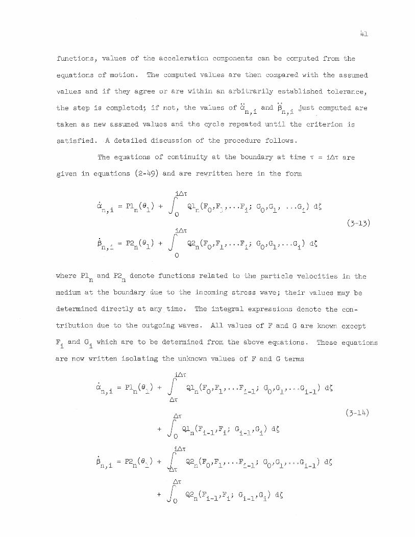
41
functions., values of the acceleration components can be computed from the
equations of motion. The computed values are then compared with the assumed
values and if they agree or are within an arbitrarily established tolerance)
the step is completed) if not) the values of a . and ~ , just computed are n,l n)l.
taken as new assumed values and the cycle repeated until the criterion is
satisfied. A detailed discussion of the procedure follows.
The equations of continuity at the boundary at time ~ M~ are
given in equations (2-49) and are re~lri tten here in the form
W'1
ct n,i Pln (E11 ) + Ia Qln(FO,Fl,oo.Fi; GO,Gl ) 00 .G.) d~
l
(3=13) i61"
~n i P2n (E11 ) + J Q2 (F 0 ) F 1 -' 0 • 0 F . ; GO)Gl " ... Gi ) d~ , n . l
0
where Pl and P2 denote functions related to the particle velocities i.n the n n
medium at the boundary due to the incoming stress wave; their values may be
determined directly at any time. The integral expressions denote the con-
tribution due to the outgoing waves 0 All values of F and G are known except
F. and G. which are to be determined from the above equations 0 These equations l l
are now written isolating the unknown values of F and G terms
ct . n,l
~n i ,
W~
Pln (el ) + J Q.ln (F O,Fl , ... F i-l; GO' Gl , ... Gi _l ) dS 61"
61"
+ 10 Qln (F i_l,F i; Gi _l , Gi ) dt;
W'1
J Q2n(FO"Fl"o.oFi~1; GO"Gl"oooGi=l) dS ~'1
Q2 (F. l"F.; G. l"G.) dS n l= l l- l

42
The integrals with limits 6'1 to ill'1 are evaluated using the numerical
technique described in a previous section.
The next step is to assume values for ex . and ~ the radial and n)l n"i)
tangential components of acceleration of the shell) from which velocity and
displacement components are determined using equations (3~12). With these
values known) equations (3-14) become effectively two equations with the two
unknowns) F. and G.) which can then be determined. l . l
The equations of motion are given in equations (2-53) and are here
written in the form
lli'1
°a n)i
= Nl(a .' ~ .) + P3 (81 ) + ~ Q3 (F) F 1) . . . F . ; GO)Gl ,,· .. Gi ) d(;; n)lJ n"l n n 0 l
(3-15) lli'1
~n i N2(a . j ~ .) + p4 (81 ) + Ia Q4 (F"Fl,,··.F.; G ,Gl
) ... G.) d(;; ) n)l n"l n n 0 l o l
from which the acceleration components ex . and ~ are now computed. If n"l n"i
the computed values agree or are within an arbitrarily establi.shed limit of
the assumed values" the step is completed; otherwise the computed values are
used as the assumed values for the next cycle of iteration.
The procedure described above requires that all parameters at '1 = 0
be known" including the initial values F and G· Initial values of velocity o 0
and displacement of the shell are specified to be zero. From the short-time
approximation presented in Section 3.7 initial values of acceleration and G o
were determined to also be zero, and the values of F to be the following o
F o
n 0
n = 1,2., ...
(3-16)
The short-time approximation also indicated that the radial acceleration
components near '1 = 0 varied as '11
/2
and the tangential components as '1 3/ 2;

43
thus to improve the accuracy of the calculations) equations (3-12) for the
first step in time were modified to
2 .. t3n 1
2 .. ex -ex "5 t3n )l n)l 3 n)l )
(3-17) 2 2 .
ex -ex t3 = - f3 n)l 5 n,l n)l 7 n)l
Without this modification) the results for the first step cannot be brought
into acceptable agreement with the short-time approximation.
The n = 0 mode is simplified somewhat because it has no tangential
component of displacement) and contains only the dilatational component of
the potential functions.
3.4 Stresses of the Shell and Medium
Solution of the equations of motion yields modal values of the
functions F and G, and the modal acceleration, velocity and displacement
components of the shell. The stresses in the shell are determined directly
from the displacements using equations (2-55) and (2-56).
Stresses in the medium at any radius and time are determined using
equations (2-57). They are here written in the form
~ 00 00
I [sn(e) + fa Tn(F)d~ + fa Wn(G) d~J n=O
where Sn(el ) represents the stress due to the incoming wave and the integral
terms that due to the butgoing Waves~. All are functions of both radius
and time. Consider the stresses in the medium for any radius equal to r at
time ~ = i6~ = i/N.
81 (Fig. 7) is now determined from the equation
81 = arc cos ~ (1 ~ i/N) (3-19 )
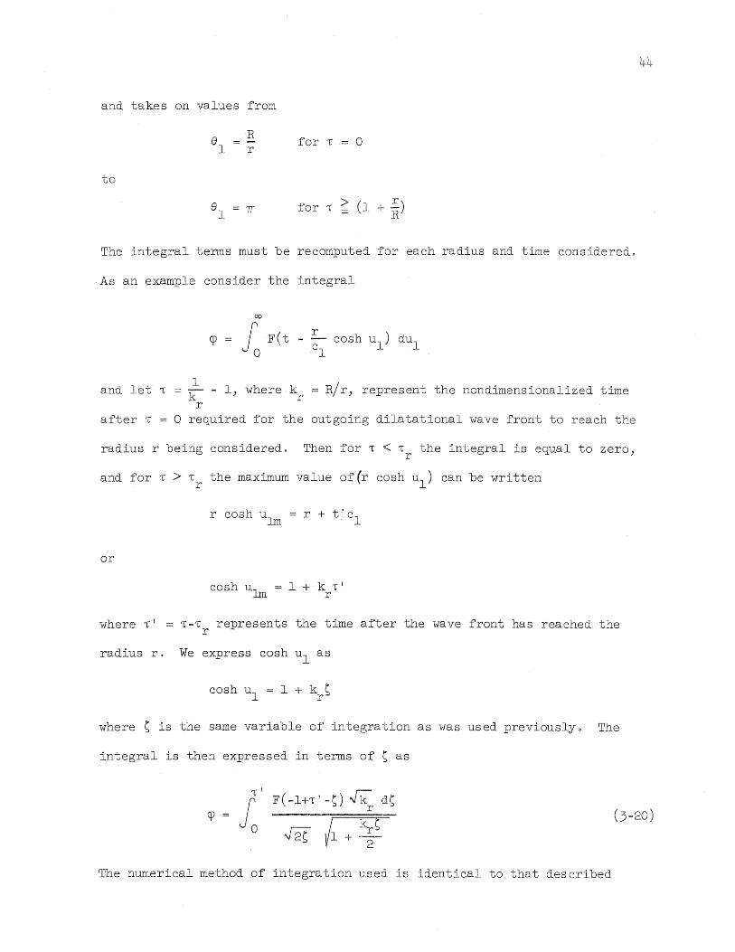
and takes on values from
to
R e =-1 r
7T
for 1" o
for 1" > (1 + ~)
The integral terms must be recomputed for each radius and time considered.
As an example consider the integral
cp
00
f F(t o
and let ~ ~ - 1) where kr = R/r) represent the nondimensionalized time r
after 1" 0 required for the outgoing dilatational wave front to reach the
radius r being considered. Then for 1" < 1" the integral is equal to zero, r
and for 1" > 1"r the maximum value of(r cosh ul ) can be written
r cosh ulm
or
where 1"' = 1"-1" represents the time after the wave front has reached the r
radius r. We express cosh ul as
where S is the same variable of integration as was used previously. The
integral is then expressed in terms of S as
44
cp (3-20)
The numerical method of integration used is identical to that described

45
earlier for the integral at the boundary, with the result that the same
weighting factors AM and EM are applicable. Note, however, that the limits m m
of the integral are now 0 to ~I j also the multiplying factor R for this m
particular integral becomes
R m
By a similar analysis, the integral of the shear potential
00
1Jr ~ ~ G( t :2 cosh u2 ) co.sh u2 dU2
can be put in the form
1;" .G(· .1 ~' S) J"kk (1 + kk S)dS -.- + -
Ia . \, . '-:k r c r c
l/r c
J k k S .J2f 1 + 2f-where
~I ~ - ~ rs
For the potential l/r
1 1 ~ ='k (- - 1) rs k c r
(3-21)
The weighting factors AM and EM remain the same but the multiplying factor m m
~ for this particular integral becomes
~D (1 + k k S ) r c r c m
k k Fr c~m
2

46
3.5 Time Dependent Stress Wave
The problem considered thus far has dealt with an incoming stress
wave with a step distribution in timeo The results obtained for the step
wave can be used through the application of Duhamel1s integral to find values
for the response of a shell and medium to incoming waves with any time
variation. As an example, a stress wave which decays exponentially with time
(Figo 8) according to the following equation is considered
er ('r) P
er (1 - .2...) e po 'riO
'[ -k -
'[ o
'[ represents the time at which the stress wave decays to zero and k is a o
parameter which is related to the shape of the curve. Stresses at any time
equal to L6rr can be found by the application of Duhamel's integral) here
written. in the form
erst is defined to be that stress resulting from an incoming step wave of
amplitude er in equation (3-22). In the numerical analysis) the time po
dependent wave is approximated by a series of rectangular sections as illu-
strated in Fig. 8.
3.6 Description of the Computer Program
The problem was programmed modewise for a high speed digital
computer (CDC 1604) using Fortran language) and considering only the first
three modes. Input data consist of the following parameters~
(1) The time intervals at which computations are to be performed)
expressed as the number of intervals required for the incoming wave to travel

one radius (one-half transit time). The degree of accuracy achieved is
dependent on this parameter) the smaller the interval the more accurate
the results. However) the machine time required for a given number of transits
of the incoming wave varies inversely as the square of the interval size ap-
proximately) thus some sacrifice in accuracy is necessary to reduce the time
of computations required.
(2) The total time over which the computations are to be performed)
expressed as the total number of time intervals to be considered. Generally
speaking) all values seemed to have reached their asymptotic (static) values
within ten transit times of the incoming wave across the cavity.
The ratio of the moduli of elastic i.ty) E IE) where E is the s s
IIplane strainfJ modulus for the shell and E the modulus of elasticity of the
medium.
(4) The mass ratio) ps/p) where Ps is the mass of the shell and P
the mass of the medium per unit volume.
(5) Poisson's ratio of the medium.
(6) The ratio of the thickness of the shell to its radius. When
considering a shell whose area) A) and moment of inertia) I) are not directly
related to the thickness) A and I must be specified separately.
(7) The amount of additional mass 'wi thin the shell expres sed as a
fraction of the mass per unit surface area of the shell.
(8) The number of radii to which stresses in the medium are
desired.
(9) The time intervals at which output data are desired.
(10) The angular increment at which output data is to be computed.
Because of symmetry only values between 0 and 180 degrees need be considered.

48
Additional input quantities in the case of the exponentially
decaying stress wave are~· and k) parameters which define the duration and o
shape of the stress pulse) respectively.
Output data consist of the acceleration) velocity) displacement)
and stress campanents af the shell far specified angles and times; and the
stresses in the medium far specified radii) angles and times.
3.7 Short-Time Appraximatian
As a check an the accuracy af the machine salutian far shart times)
the boundary equatians and the equatians af matian were salved appraximately
by making a series expansian af all pertinent functians in terms af time as
the independent variable. Althaugh the fallowing discussian is limited to' the
case af the incaming dilatatianal wave) the basic principles are the same far
either of the types af wave CODS idered.
The expressi.ans far the velacities and stresses in the medium
araund the baundary due to' the incident wave all have been written thus far
in terms af 81
, the pasitian angle af the wave. In terms af nandimensianalized
time 1") all functians af 81 can be written in terms af ~ using the fallawing
relatians
cas el
1 - ~
r 1 1 2 .. oJ sin e = ~Ll = 1+ ~ _ - 'T - (3=24) 1 32 "
81 = - [ 1 3 2 ~ 2~ _1 + 12 ~ + 160 ~ + 0.0 J
The integral values representing the effects af the autgaing waves
are alsO' expressed as functians af 1". The fallawing example will illustrate
the technique used to' accamplish this. Far example) cansider the transfarma-
tian af the integral

cp
.00
f F(t o
49
As was shown in Section 3.2) cosh u l in the integral varies in value for any
given time ~ from 1 to 1 +~. It is convenient for purposes of analyzing the
integral to represent the variable cosh ul as follows
cosh ul = 1 + W~
where ~ is now a fixed value in the integration and w is defined as the
variable of integration whose value ranges from 0 to 1. The function
F (-1 + ~ (l-w ) )
is expanded in terms of a power series as
F( -1 + ~(l-w))
where Y. are unknown coefficients of the series. Since l
·l21 [ Wf" 3 2 ] dUl 2~ 1 - ~ + 32 (w~) + ... dw
the integral can now be written as
from which after performing the indicated integration
]
(3-26)
The integrals which represent the effects of the outgoing shear
wave can also be transformed in somewhat similar manner. Consider for example
the integral

50
00
ljr J' G( t - ~ cosh u 2 ) cosh u2 dU2 o '2
In this case cosh u2
varies from 1 to 1 + k ~ where k c c
Therefore we write
cosh u = 1 + wk ~ 2 c
(3-28)
where w is now the variable of integration ranging in value from 0 to 1 in
the integral. The function
1 G( - k + ~ (l-w))
c
is expanded in terms of a power series as
1 G( - k + ~ (l-w) )
c
i )i E.~ (l-w l
where Ei are unknown coefficients of the series. From equation (3-28)
The integral written in terms of the variable w is now
~ Jl [ J [1 + k W1"
... J [1 + WkcTJ dw ljr = _c_ l Go + El~(l-W)+,. 0
c ~4-. - +
.J2 0 rw-and performing the integration
. [2 2 4 ljr =.J2k
C1" 1"(3 Go) + ~ (15 El + .-l.k
10 c Gol + T3( ... J (3-29)
The same basic technique is applied to all the integrals so that now the
effects of both the incoming and outgoing waves can be written in terms of T.
Substitution into the continuity equations and the equations of motion yield
the following for any mode

51
00 1
I i - 2
a fl. (F, G) 1" l
i=l
00 1
I i· - 2
f3 f2. (F,G)1" l
i=l (3-30)
00 1
I i - 2
a + £l.(a,f3) f3.(F,G)1" l l
i=l
00 1
L i -
2 ~ + £2. (a,f3) f4. (F,G)1" l l
i=l
where fl., f2., f3., and f4. are coefficients which contain certain elements l l l l
~~ ~ - ~..p Cl.lll..l \::.. UJ. known functions
l
of the displacements.
To solve the above equations, the displacement components of the
shell are expressed as Frobenius (8) type series
.iX>
I c+i a p.1" l
i=l
00
\" c+i f3 L q.1"
l
i=l
where p., q., and c are unknown coefficients. Substitution into equations l l
(3-30) results in the following set of equations
00 CXJ 1
I 1"c+i-l I i
2 Pi ( c+i) fl. (F, G) 1"
l
i=l i=l
00 00 1
I c+i-l I i ~
(c+i) f2. (F,G)1" 2
(3-32) qi 1" l
i=l i=l

52
00 00 00 1
L c+i-2 L c+i L i
2 Pi (c+i)' (c+i-l) 1: + £l(p." q. )rr f3.(F"G)1:
l l l
i=l i=l i=l
00 00 QO 1
~ c+i-2 L ( ) " c+i L i
2 qi (c+i)·(c+i-l) 1: + £2 p." q. ' rr f4; (F" G) 1:
l l l
i=l i=l i=l
The coefficient c is now determined by inspection. Then through a step by
step process which involves the equating of coefficients of like powers of 1:"
values of p., q.) /.) and E. are determined. The following equations are then l l l l
used to find values of the potential functions" and the displacement components
of the shell.
00
F(1:) F L i + /.1:
0 l
i=l
00
G(rr) G L i + E.rr
0 l
i=l
00 (3-33)
a(1:) L c+i Pi 1:
i=l
00
t3(-r) L c+i q.1:
l
i=l
Velocity and acceleration components may be determined by differentiation of
the above expressions for the displacements.

4.1 General
CHAPTER: IV
DISCUSSION OF RESULTS
Results of computations performed to determine the effect of the
various parameters are discussed in this chapter.
53
Although equations presented throughout the study have been written
to include an infinite number of modes) the greater part of the actual calcu
lations performed and presented here are the results obtained considering only
the modes n = 0, 1, and 2. It is important to note that during envelopment of
the shell by the plane stress wave, a Fourier series representation of the
incoming wave is objectionable in that the series at this stage is slowly con
vergent, thus necessitating a large number of modes to accurately represent the
plane wave. However, after passage of the wave across the cavity, the Fourier
expansion of the incoming stresses around the boundary results in coefficients
of all modes except n = 0 and 2 becoming identically equal to zero for the
plane dilatational wave) and coefficients of all modes except n = 2 becoming
identically equal to zero for the plane shear wave. Therefore, stresses due
to the outgoing waves in modes corresponding to those of the incoming wave
whose coefficients become zero must also eventually vani,sh at long times 0 The
limited study conducted for modes greater than n = 2 indicated that the
maximum effect of the higher modes occurs within one transit time of the
incident wave and rapidly decays) thus contributing relatively little to the
maximum response of the shell which occurs after several transit times.
However, for determining the early time response of the shell and medium)
the higher modes are significant and should be considered in further extension
of this work.

54
In the tables and figures to be di.scussed, quantiti.es given in
non-dimensionalized units are defined by equations (2-36) and (2-50). Stresses
are given in units of the absolute value of the amplitude (/a I or ja I) of the p s
incident wave; a negative stress means a compressive response to an incoming
compressional (Fig. 1) or a positive shear wave (Figo 2). The physical
properties of the shell relative to those of the medium) as well as the nature
of the incoming wave are indicated on the graphs. Unless otherwi.se stated,
the shell is considered to be an unstiffened one so that its cross sectional
area and moment of inertia are related to the thickness as given by equations
(2-52). Except where indicated) there is assumed to be no additional mass
within the shell. Numeral subscripts denote the mode number.
The shell and medium have been assumed to exhibit linearly elastic
behavior thrDughout their stress histories) which for the practical problem
does not permit evaluation of any spalling or non-elastic effects.
Values of stresses given are in addition to those which exist prior
to the arrival of the incident wave. For the elastic case) the effect of
prior stresses such as those resulting from the overburden may be taken into
account by merely adding them to stresses caused by the incident wave.
For clarity of presentation and because of the impracticability of
including solutions for all possible permutations of the parameters involved)
the discussion in this chapter is limited to a few representative cases,
402 Modal Response of the Shell and Medium
Figures 11 and 12 illustrate the shape of the modal components of
the dilatational and shear potentials obtained in the solution to a typical
problem. It appears that a singularity occurs at one transit time in the
case of the F functions resulting in the slight irregularity of the curves at

55
this point. Since computed values of stresses were determined to be rather
insensitive to relatively large variations in values of the F and G functions)
the effect of the irregularity would seem to be slight.
Figures 13 through 20 show modal acceleration) velocity) displace=
ment and stress components for the shell and stress components for the medium
at the boundary) as they vary with time. Static values shown were computed
using the method given in Appendix B.
The high accelerations ,computed near the beginning are not truly
representative of the actual case, since they are the result of assumptions
made earlier in deriving the equations for the shell. The shell was repre
sented by a line describing its mi,ddle surface which permits no variation in
accelerations) velocities) and displacements of particles through the actual
thickness. Also) no provision was made for refraction of the incident wave
through the shell lining. These limitations restrict the applicability of
the solutions to a shell whose thickness is small relative to its radius.
The n =1 mode is primarily a translational one which accounts for
the rigid body translation of the shell after it has been enveloped by the
incident wave. Thus) it can be seen that the velocity components for this
mode approach constant values equal to the velocity of the medium behind the
incident wave front) and displacements grow wi,thout bound reaching a straight
line variation with time. Note that the stresses contributed by this mode
reach their peak values within one transit time and quickly damp out)
approaching zero asymptotically. For the incident shear wave) the n = 0 mode
is also a rigid body movement which accounts for rigid body rotation) and
contributes little to the stresses.
Modal quantities obtained are coefficients of Fourier series;
therefore) the total response or effect is determined by adding the coeffi,cients

multiplied by the appropriate sine and cosipe terms for any desired angle.
Figures 21 through 24 show the time variation of stresses in the shell and
medium for various angles when the first three modes are summed. The maxi
mum stress in the shell for any angle may be determined by adding the bending
stress to the hoop stress. This is indicated in Figs. 21 and 24 by the
dotted line above the hoop stress.
Figure 25 is given to illustrate the relative magnitudes of the
hoop stresses in the shell and medium for several thicknesses of shell. This
also shows the effect of varying the relative thickness of the shell on the
hoop stress in the medium. The dotted line indicating the hoop stress in
the medium for an unlined cavity was obtained from the report by Paul (6).
Figures 26 and 27 show how the relative thickness of the shell
affects the radial and shear stresses in the medium.
As was discussed earlier) stresses in the medium for any radius
can be determined by reevaluating the integral terms which represent the
effects of the outgoing waves) and adding them to the Fourier expansion of
the incident wave. Figure 28 shows the modal and total radial) hoop) and
shear stresses which were computed for a time equal to 10 transit times.
These values are compared later with the static stresses) but on this figure
the static stresses do not differ by more than the thickness of the lines)
and therefore are not shown. The time variation of the radial and hoop
stresses in the medium for various radii are shown in Fig. 29 for the incident
dilatational wave) and in Fig. 30 for the incident shear wave.
4.3 Short-Time and Asymptotic Comparisons
A method for obtaining a solution to the problem which is accurate
for very short times (T « 1) was presented in Section 3.7. This was desirable

57
to validate the machine solution and to determine the effect of the size of
time interval selected. The results for a representative problem are shown
in Figs. 31 through 33 for the incident dilatational wave, and in Figs. 34
through 36 for the incident shear wave. Four terms of the series representing
the F and G functions, and three terms for other quantities were used in the
short-time solution.
As can be seen from the graphs, good agreement was obtained for
very small values of time, somewhat shorter time being obtained for the shear
wave as compared to the dilatational wave. The shorter time results from the
nature of the forcing functions (Eqs. 2-19 and 2-32) which indicate a more
rapid rise in the incoming stresses for the incident shear wave.
Within the range of time for which the short-time solution is valid,
decreasing the size of time interval for each step of the machine solution
resulted in closer agreement between the two methods, as is to be expected.
It also indicated that the stresses and displacements are not as sensitive to
variations in the interval size as are the F and G functions.
At the other end of the time scale, i.e., at a relatively long time
after passage of the incident wave front across the cavity, another check on
the accuracy of the machine solution is afforded by the asymptotic approach
of all values to the static results. Figures presented thus far have shown
that the static condition is approached well within ten transit times.
The time interval used in the machine solution affects the stability
of the results for long times. This is indicated in Fig, 37 which shows the
variations in computed values of the displacement components for mode n = 2
at relatively long times, for different time intervals. N represents the
number of time steps required for the incident wave to travel a distance equal
to the radius of the opening, and liN defines the interval size. Note the

smaller graph which shows the percentage difference between the computed
values at ten transit times and the static values.
As the interval is decreased the machine solution at long time
approaches the static solution more closely. Below a certain size of time
interval) there is little difference in the results) which indicates asymp
totic convergence to the correct solution. For this particular problem)
N r;;;: 30 seems to be UcriticalU in that for N < 30) wide variations in computed
values occur. As the mode number increases) the Hcritical" value of N in=
creases rapidly, and the requirements of computer storage and calculation
time become decisive factors which make impractical the study for long times
of modes much larger than 2. The interval size selected for all problems
solved (exclusive of the study to determine the effect of the interval size)
was set equal to 1/40 (N = 40) of the half transit time of the i.ncident waveo
For the static case) only the modes n = 0 and 2 yield values other
than zero. Table 1 compares values of shell stresses and displacement com~
ponents in these modes obtained from the computer solution to a particular
problem at a time equal to 10 transit times) with the stati.c solution. Most
pairs of values differ by less than one percent. Comparable agreement of
stresses in the medium at various radii are shown in Table 20 Values in
Tables 1 and 2 were obtained from the solution to a problem whose parameters
were~ ~E = 4.0) ~p = 3·0) ~t =. .05) and V = .250
Although the figures and tables presented above were for a particular
problem) the discussion given is applicable to all problems which were solvedo
Changing the physical characteristics of the shell and medium 'ivi thin the range
of values studied had hardly any effect on the degree to which the long time
machine solution and the static solution agreed. Also) the absolute value of
all quantities which should asymptotically approach zero became less than
.00005 in each case well before ten transit times.

59
4,4 Effect of Parameters
Studies were conducted to determine the effect of each of the
following parameters:
E Ps s 11E 11p -E p
t (mediwn) 11 = ~ V V t R
for an unstiffened shell without additional mass, Since it was impractical
to take into account all permutations of the above parameters., a basic shell
where
4.0
V .25
was considered from which each parameter was separately varied to determine
its effect on the resulting stresses and displacements, Calculations
performed were only for the case of the incident dilatational (p) wave,
Of particular interest was the determination of the maximwn dynamic
stresses and displacements (not including rigid body translation) due to the
incident stress wave. Tables. 3 through 6 compare the maximwn values obtained
in the machine solution with the static solution 0 IIDLF)II termed the dynamic
load factor) is defined as the factor by which the displacement or stress
produced by 0 applied as a static load should be multiplied in order to obtain p
the maximwn dynamic value. Figures 38 through 41 are given to graphically
illustrate the variations in stresses and displacements) both static and
dynamic) in the range of parameters considered. Stresses are given in units
of 10 I and displacements in non-dimensionalized units defined by equations p
(2~36) and (2-50).

Table 3 and Fi.g. 38 illustrate the effect of increasing the
relative thicb1ess of the shello The range of values selected for ~t is
probably much greater than is practical or justified by the assumptions of
60
the analysis) and was considered only to determine the trend of the results.
As ~t is increased) displacements and hoop stresses of both the shell and
medium decrease; however, the bending stress of the shell and the radial and
shear stresses in the medium at the boundary increase. Figure 25 shows the
time variation of the hoop stress in the shell and medium for various thick-
nesses of shell) including the case of the unlined cavity.
Increasing TIE results in a rapid increase in the displacements and
stresses of the shell and a much lower rate of attenuation of the hoop stress
in the medium. See Fig. 39 and Table 4.
Table 5 and Fig. 40 show that the parameter ~ has no effect on the p
static results but does affect the dynamic response.
the maximum response in both the medium and shell.
Increasing Tj increased p
Figure 41 and Table 6 show that within the range of Poisson!s ratio
for the medium considered) as V increases displacements and stresses in the
shell decrease) with very little additional reduction of the medium hoop
stress.
Additi.onal mass within the shell was shown to contribute relatively
little to the overall response. This is mainly due to the simplifying assump-
tions which were made in deriving the equations of motion to account for the
additional mass. Figure 42 shows the effect of the presence of additional
mass equal to 40rr times the mass of the shell on the dynamic response of a
particular shell. Additional mass decreases the displacements and increases
the dynamic stresses in mode n = 1.

61
4.5 Response to Time Varying Incident Wave
The results obtained from a solution to an incident wave with a step
variation iiltime was shown to be 1.1se,fulbYapplication of Duhamel is integral in
determining the response to any time varying stress wave, The case of the
exponentially decaying wave was considered, the results of 'which are
illustrated in Fig. 43. Substantial reductions in the maximum stresses can
be expected as the duration becomes smaller. In Fig. 44 is shown the effect
of a linear rise in the amplitude of the incident wave. Note that for a
wave with a linear rise followed by a step variation in time, very li.ttle
decrease in maximum stresses occurred.
4.6 Comparison with Previous Work
Baron (1), using a different method of analysis., investigated the
dynamic response of two shells with different physical characteristics sub-
jected to an incident plane dilatational wave. Figures 45 through 49 compare
his results for the modal values of stresses and displacements of the thin
shell, with results obtained by the method of solution given in this study.
Similar results were obtained considering his so-called stiff shell. Although
the shape of the response curves can be considered similar in the two reports)
the magnitude of the dynamic response in Ref. (1) seems consi.stently higher
than in the present report, and the long time results asymptotically approach
values higher than the static solution. The following table compares the
maximum modal stresses) for Poisson's ratio of 0.25) obtained in the two reports)
and also shows values for the static case . Stresses are given i.n units of
/a /. The bending stresses for the stiffened shell cannot be compared directly p
since d, the distance from the neutral axis of the shell to its extreme fiber,
is not stated in Ref. (1).

62
Thin Shell Stiff Shell
Maximum Stresses Maximum Stresses
Ref. Current Ref, Current Quant 0 Mode (1) Work Static (1) Work. Static
(Jee 0 -4·79 -4.56 -4.10 -4·79 -4.08 ""3.67
(Jee 2 4.69 4.11 3·67 3·42 3·20 2·95
a sb 0 0.043 0,043 0.039 0·55 4.08d 3·67d
a sb 2 0.140 0.137 0.122 1·70 13·29d 11.89d
4.7 Conclusions
Conclusions drawn from the results of the analysis are~
(1) The method which has been presented is p~actical for effective
computation of the dynamic response of a cylindrical shell embedded. in an
elastic medium when subjected to plane dilatational or shear waves. The
solution presented herein is believed correct since it was check.ed by independent
methods at short and. long times.
(2) Peak stresses and displacements in both the medium and shell
occur sometime after the transit of the incident 'wave across the cavity.; of
the problems solved" both the average and mean time at whi.ch the peak values
occurred was equal to 3 transit times. The dynamic effect measured in terms
of the ratio of the maximum stresses and di.splacements to the static values
varied within a relatively small range. The average value of this ratio was
1.12 and the mean" 1011. Thus" for the cases considered at least" the maximum
stresses and displacements to be expected for a particular situation can be
roughly approximated by determining the static values and by multiplying them
by a factor of 1.1.

(3) The largest stresses in the shell occurred for a relatively
thin liner in a medium with a low modulus of elasticity) low mass density)
and low Poisson's ratio. The greatest reduction of the hoop stress in the
medium as compared to the unlined cavity results from a relatively thick
liner in a medium with low modulus of elasticity and high mass density.
Additional mass within the shell has relatively small effect on the dynamic
stresses.
(4) The practical value of tunnel linings to reduce the maximum
stresses in the medium depends on the several conditions mentioned above) and
on the magnitude of the incident stress wave. Under favorable conditions,
reduction of stresses on the order of 30 percent or more is possible. However,
for materials such as granite) smaller reductions can be expected for steel
liners of practical size.
(5) Certain assumptions made concerning the behavior of the shell
have limited the applicability of the analysis to relatively thin liners.
Future studies of the behavior of thick shells would indicate the effect of
the approximations used herein. The analysis has also been based on the
assumption that the behavior of both the liner and medium is linearJ~ elastic
at all times. Perhaps a more desirable condition would be one in which some
inelastic behavior is permitted to take place in the medium surrounding the
shell or in the shell, or one in 'which some inelastic energy absorbing medium
such as cinders or foamed plastic surrounds the shell. As a subject of future
study) it is recommended that the behavior of thick shells" and thin shells
surrounded by some energy absorbing layer) be considered.
BIBLIOGRAPHY
1. Baron) M. L.) and Parnes) R., Diffraction of a Pressure Wave by an Elastically Lined Cylindrical Cavity in an Elastic Medium) The Mitre Corporation) Bedford, Masso, December 1961.
64
2. Flugge) W., Stres sesin Shells., Springer~ Verlag, Germany., 1960" pp 0 4780
3. Kolsky, Ho) Stress Waves in Solids, Oxford~ Clarendon Press) 19530
40 Lamb, H., Hydrodynamics, Dover Publications, New York) 1945) pp. 296-301) 503-505) 524-527-
5. Newmark) N. Me) A Method of Computation for Structural Dynamics) Journal of the Engineering Mechanics Division) Proceedings of the American Society of Civil Engineers, Vol. 85) No. EM3, July 1959.
6. Paul) S. L.) Interaction of Plane Elastic Waves With a Cylindrical Cavity) Ph.D. Dissertation) University of Illj.noi.s) 19630
7. Robinson) A. R.) Structural Effects of a Shock Wave Incident on a Cylindrical Shell, M.S. ThesiB) University of Illinois" 1953.
8. Spiegel) M. H .. , Applied Differential Equations, Prentice~Hall) Inc.) Englewood Cliffs, New Jersey, 1958 ) pp. 263-270.
9. Timoshenko, S') and Goodier) J. No) Theory of Elasticity) McGraw=Hil1 Book Company, Inc., New York) New York, 1951) pp. 58=80.

APPENDIX A
DERIVATION OF THE EXPRESSIONS INVOLVING THE POTENTIAL FUNCTIONS
A.l General Form of the Potential Function
The dilatational potential function must satisfy the wave
equation
(A-l)
~ in the case of the incoming dilatational wave is an even function of e and
thus can be expressed as a cosine Fourier series
cp
ao
I fn(r,t) cos nB
n=O
(A-2)
where f is a function of rand t representing the modal coeffi.cient of the n
potential function. By substitution of the above expression into equation
(A-l) we obtain the equation that must be satisfied by f . n
The general solution of f is assumed to be of the form n
f = rn R (r,t) n n
Then R is some function of rand t satisfying n
(A~3)
(A-4)
(A-5 )
IfR is a solution it can be shovm that the corresponding equation for n
R 1 is satisfied by n+
1 dRn R ---n+l - r dr

By repeated application of this result it can be shown that equation (A-5)
is satisfied by
where R is the solution of o
66
(A-8)
The solution to this equation for the case of a wave diverging from a center
is
00
R o J(o F(t ~l cosh uI ) aUI (A-9)
For the proof of this) see Lamb (4)0 Therefore) the coefficient f of the n
potential function is written as
00
rne! ~) n f F(t f
r cosh ul
) dU1 -n r dr cl 0
(A-IO)
For modes 0) 1) and 2) this can be written
00
f f F(~l) dUl 0
0
00 00
where primes indicate the derivative of the function F with respect to its
argument. Note that the expression for the n = 2 mode contains derivatives
of two different orders 0 It is convenient to express the function f in n
terms of derivatives of a single order which may be done through integration

by parts. For the n = 2 mode we then wish to change the second integral to
an integral involving the second derivative of the function F. Integrating
by parts gives
where
Thus
00
f F' (~l) cosh u l dUl o
dTJ
The second term can be shown to equal zero since for its lower limit
sinh ul
= 0; and for its upper limit) FI is the integral of the function r at the wave front which under the assumed initial conditions) does not exist.
Therefore) the coefficient of the potential function for the n = 2 mode can
be written as
00
f F" (t o
(A-II)
By a similar process the coefficients of the potential function for any other
mode can be reduced to the form
f n
The shear potential function must satisfy the wave equation
(A-12)
(A-13 )

68
Ijr in the case of the incoming dilatational wave must be an odd function of e
and can be represented as
00
1jr L gn ,t) sin nB
n=l
and proceeding exactly as in the case of the dilatational potential the
general expression for the coefficient g is found to be n
00
(\_l)n J . Gn(t n
c2
0
Ao2 Velocity Terms
(A-14)
The equations for the velocity components of a particle on the
boundary due to the outgoing waves are
(A-15 )
The components of velocity and the potential functions are expanded in series
as
00
u }' ;,. (rJt) cos ne L.....J n
n=O
00
v L b (r,t) sin ne n . n=l
00 (A-16)
cp L f (r)t) cos ne n
n=O
00
Ijr }' g (r)t) sin ne L-1 n
n=O
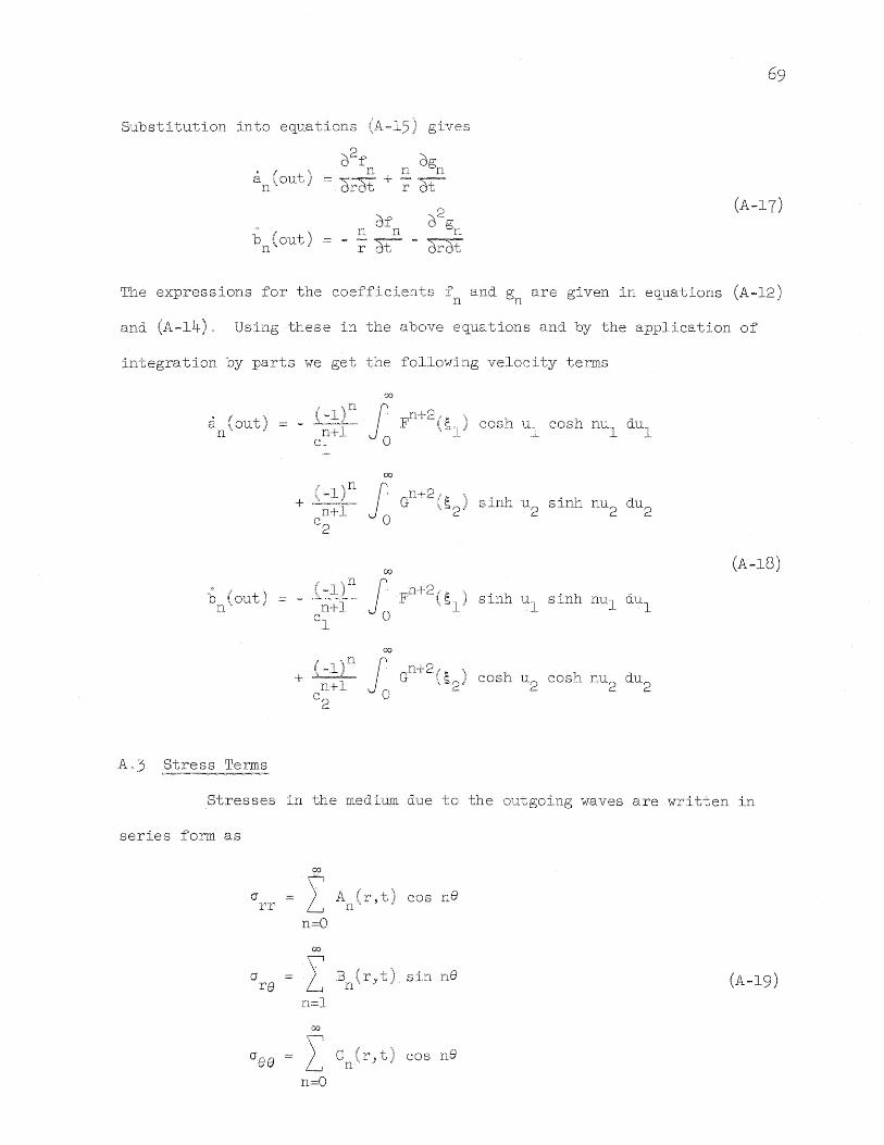
Substitution into equat,ions gi.ves
(A-17)
b (out) n
The expressions for the coeffic.ients f and g are given in equations (A-12) n n
and (A-14)0 Using these in the above equations and by the application of
integration by parts we get the following velocity terms
a (out 'Ii n·
b (out) n'
Ao3 Stress Terms
+ (_l)n '\ '
n+l' c
2
00
cosh ul cosh nUl dUl
00
J 0 "s'2) s:inh u2 sinh nU2 dU2
00
J o si,nh ul sinh nUl dU
l
(A-l8 )
Stresses in the medium due to the outgoing waves are wri.tten in
seri.es form as
00
a I A (r,t cos ne rr n" ,
n=O
00
a y B (r~t) sin ne (A-19 ) re '---J n' ,
n=l
00
Gee I C :(r9t) cos ne n ' n=O

70
By substituti.on into equations (2-10) the coefficients A J B ) and Care n' n n
expressed i.n terms of the coeffici.ents of the potential functions., fn and gn
d2
f d ng~J A (out) + 2f-t)
[ n n gn ~~2= + r dr -n dr r
"- [Mn + ~ 2 OgnJ n
f + ~ g - - n r dr r n r n dr
B (out) n
~f ~2 2 ~
[ 2n 0, n ,+' 2n f 0 gn n + .-h OgnJ
~ ~_= Jr dr 2 n - ---2= - ~ gn r dr r dr r
(A-20)
( ) =: A,+,2fJ, [dfn + !2: g _ n2 f C : out, ~
n r ur r n r n
dg -"1
nJ n ~= dr
+ A, [02fn + ~ Ogn _ n.:n2J -dr2 . r dr ~
Again,!l using the equations for fn and gn given earlier 'we can write the above
coefficients finally as
A (out) n
B (out) n
c (out) n
<Xl
(-l)nf-t J' Fn+2( 1:1
) [,,- 2 ] n+2. 0 ~ ,. cosh nUl _~ + 2 cosh u l dUl cl
00
(-l)y (. Gn+2 ( ~2) sinh 2u2
sinh nU2
dU2 n+2. v 0 -c
2
( . n
_ l.-l)j:l n+2
c2
00
J. Gn+2 (1:) 'h h \s2 cos_ nU2
cos 2u2
dU2 o

71
APPENDIX B
STATIC SOLUTION
B.l Dilatational Wave
The static solution presented here is based on the application of
the theory of stress functions presented by Timoshenko (9). Under static
conditions) it can be assumed that at large distances from the boundary of
the cavity the state of stress in the medium is equal to the stress field in
the medium behind the front. In polar coordinates this is
a _ (l+V) a - (l-v) a cos 2e rr 2 p 2 P
are (l-V) a sin 2e (B-1) 2 P
aee (l+V) a + (l-V) a cos 2e
2 p 2 P
a is the stress in the medium in the direction of wave propagation and vo p P
is the stress parallel to the wave front. v) derived from the assumption
that there is no strain parallel to the wave front) is equal to
v ..L l-v
(B-2)
It can be seen from equations (B-1) that the n = 0 and 2 modes describe
exactly the free field stresses. Therefore) the unknown stresses at the ed.ge
of the cavity can likewise be expressed in terms of these modes
where po) P2
) and S2 are the unknown modal components of stress acting at
the boundary. These same stresses must act on the shell. Thus the boundary
stresses in the medium and shell can be illustrated as shown in Fig. 9.

72
The e~uations of e~uilibrium in the medium under plane strain
conditions are satisfied by the following expressions for the components of
stress
where n is the stress function in terms of rand e.
B.ll n o Mode -----
The general solution of the stress function for the n
given by Timoshenko as
2 n = K log r + Mr
from which can be derived the stress components
k cr =-2+2M rr
r
o
k cree 2" + 2M
r
(B-4)
o mode is
(B-5)
The coefficients K and M are determined from the states of stress at r ~ 00
and r = R
(B-6)
For the conditions of plane strain) the strains are

73
E = l [a = v aee] r - rr E -
Ee = ~ [aee - v arr] (B-7) E _
1 l rEi - are !-l
where
E E
modulus of plane strain 2
1 - V for the medium
Displacement components are found by suitable integration of the following
equations for the strains in the medium
E r
dU dr
1 dU dV lre = r de + dr
v r
Displacements in the medium for the zero mode are
u R
v R
(l+V)
E
o
(B-8)
(B-9)
The corresponding displacement components of the shell with an exterior
compressive force P are found in Flugge (2) to be o
u P R s 0
R - =-EA s
v s 0 -=
R
where E E s
modulus s 1 - v2 for the s
(B-1O)
of plane strain shell

74
The unknown stress P is now determined by equating the radial displacement o
components, to get
(l+V) a p :e
0
[: R v] ._+ 1 + A
s
(B-ll)
After P is determined" stresses in the medium at any radius can be found o
using equations (B-5)o Equation (B-10) gives the displacement of the shell;
and the hoop and bending stresses of the shell are) respectively
P R o
(j e.e =--;;:-
B.12 n 2 Mode -----
(B-12)
The general solution in terms of a stress function Q is given as
n = [kr2 + M2 + N] cos 28 r
from which the stress components in the medium become
[ 6M 4NJ cos 2e a - 2K+'4+-"2 rr - r r
aee [ 2K + ~J cos 28 r
[2K _ 6~ 2NJ . 2e are -"2' Sln - r r
(B-13)
Coefficients are determined as before from the states of stress at r ~ 00
and r = R
(B-14)

75
R4 [3(1-V) ] M b 2 a p - P 2 - 282
The displacement components of the medium at the boundary can be expressed
as
u R
v R
1 [ -= -=- 2(v-l) E -
= ~ [2(1-V) - 2(2-v) p - (5-v) 8 ] sin 2e E _ 3 2 3 2
and the corresponding components for the shell are
u s
R
v s
R
[_ P2 ~~ _ 32 R
3] cos 2e
_ E E s s
[_P2 ( R3 R 181 + 6A -E
s
(B-15)
(B-16)
The unknown boundary stresses P2
and 82
are determined by equating the dis
placement of the shell and medium at the boundary. The hoop and bending
stresses in the shell are then found from the following equations
P2R 282R
aee = (-+-) cos 2e 3A 3A
tR3 (B-17) 0"8B = 121 (2P2 + 82) cos 2e
Displacements of the shell and stresses in the medium can be determined us~ng
equations given earlier in the discussion. Total static stresses and dis-
placements are merely the sum of the modal values for any angleo

B.2 ShearWave
The free field shear wave stresses expressed in polar coordinates
include only the n
(J rr
2 mode
(J sin s
0 cos s
-0 sin s
261
261 (B-18)
2e
where (J is the amplitude of the incoming wave. The static solution is s
obtained exactly as in the case of the dilatational wave except for the
interchange of sines and cosines resulting from the difference in geometry.
The resulting e~uations are
a. Displacement components
u s "If
v s
R
sin 28
b. Shell Stresses
c. .Medium Stresses
cr rr
(2A + 6c + 4D) sin 28 4 2
r r
_ (2A _ 6~ r
2D) cos 28 2
r
(fee (2A + 6~) sin 28 r
(B-19)
(B-20)
(B-2l)

where
A a
s 2
In the machine program) the n = 0 mode is purely rotational and
77
thus we get a static value of tangential displacement. This is calculated
as follows
e 1 1 Os Y"ot
= - )' 2 2 xy lJ.
(B-22)
1 (J
v e s -R rot 2 lJ.
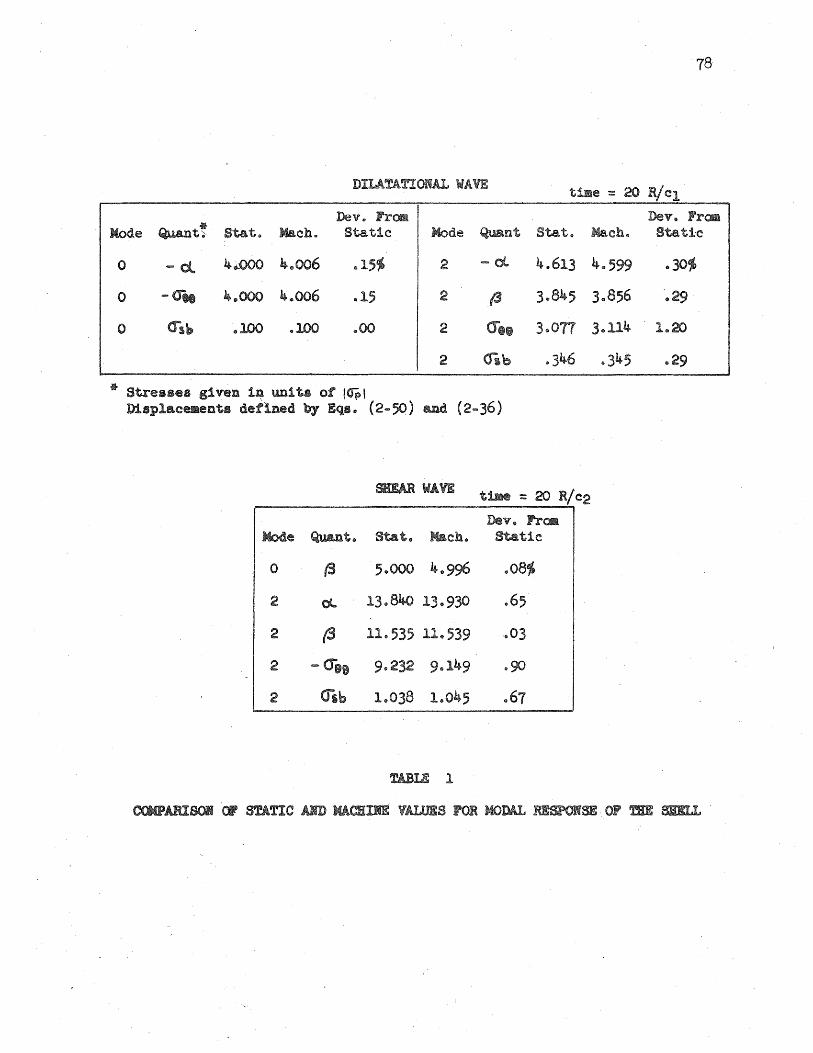
78
DILATATIONAL WAVE tble :: 20 RI c1
Dev .. From DeVil P;roa Mode '* Quant~ Stat. Mach .. Static Mode Quant Stat. Mach. Static
0 -ol 4~OOO ~.oo6 .. 15~ 2 -ot 4.613 4 .. 599 .30~
0 -cr" At..OOO 4 .. 006 .. 15 2 t3 3 .. 845 3 .. 856 .. 29
0 CTsb .. 100 .. 100 .. 00 2 300n 3 .. 114 1 .. 20
2 OSb .346 .. 34; .29
* Stresses given 1~ unit. of lapl Di8plac~ents defined by Eqs .. (2-50 ) and (2-36)
SHEAR WAVE time :: 20 R/C2 Dev. Free
Mode Quant 0 Stat. Macho Static
0 (3 5 .. 000 4.996 ,,08tj
2 Ol. 13 .. 840 13 .. 930 .65
2 (3 110535 11 .. 539 .• 03
2 -(Tee 9.232 9 .. 149 .. 90
2 (jsb 1.038 1 .. 045 .67

79
DILATATIONAL WAVE
1.0 R 2.0 R 3.0 R 4 .. 0 R
Mode Quant! Stat .. Mach .. Stat. .Mach" Stat" Mach .. stat .. Mach ..
0 ... a;.", .. 200 .. 200 .. 550 0551 ,,615 .. 616 .. 638 ,,639
0 ... 1,,133 1.135 .783 .. 785 .. 718 .. 720 .. 696 .. 697
2 ... errr ... ,,153 "".155 "Ill .112 .. 226 .229 .. .. 273
2 (T"" " .307 ~312 .. 428 8429 .. 384 .386 .. 363 .. 366
2 cree .. 872 .. 868 .367 ,,368 .. 340 ,,342 .. 335 ,,337
*' Stresses given ill units of IfPl
SHEAR WAVE time :: 20 HI c2
1,,0 R 2.0 R 3,,0 R 4100 R
Mode Quant 10 State Mach .. Stat. Mach. Stat., Mach., stat ..
2 0'; \V; -.460 -,,455 .. 332 .331 ,,675 .. 678 .814 .. 815
2 aye .. 921, .913 1 .. 283 1 .. 286 1 .. 151 1 .. 154- 1 .. 092
i 2 -<r" 2.616 2.636 1,,101 1.104 1 .. 020 1 .. 022 1 .. 006 1 .. 009
TABLE 2
COMPARISOJI OF STATIC AIm MACHmE VALlJES FOR MODAL STRESSES

.01
.. 10
.. 15
'lJt .. 01
.. 05
.. 10
.. 15
.,20
'?t 1901
.,05
el0
.15
020
..
,,9,,21 -10,,12
-7 .. 08 ... 7 .. 74
-5 .. 56 - 6 .. 15
-4 .. 60 - 5021
-3,,94 - 4e52
(f,b (90°) J Static_J Max ..
.. 10 .. 11
.. 45 .. 50
.. 83 .. ~
1,,18 1.,36
1 .. 50 1076
1~1O 3~12
1 .. 09 2 .. 88
1910 2,,25
1 .. 13 2,,25
1 .. 14 2 .. 25
-2 .. 49
... 2 .. 01
-1 .. 67
-1 .. 45
-1$30
-1,,84
80
1 .. 09 3 .. 13
1.09 2 .. 88
1 .. 11 2.25
. __ . __ ._----_._----.--- --
DII
-r------rr-----------------:--~
I ~-~~~--~ tm , Static 1 :Max ! m..r tm
-' ----_._- --. --~ - -1 .. 11 3 .. 38 '" G09 ... ,,10 1,,10 3 .. 25
1 .. 11 3 .. 25 - .. 35 - .. 39 1 .. 11 2.88
1 .. 13 3 .. 00 ... • 55 ... .. 63 1,,14 2 .. 50
1 .. 15 2088 ... .,68 "" .. 79 1 .. 17 2.50
1 .. 18 2 .. 88 ..... 75 GO 991 1 .. 21 24150
d.. {Oe} ---1---~- I __ ~J StatiC~ t5~1-:T-' Static -1 ___ -9.65 ... 10 .. 64- 1.,10 3., 4 .. 67 5 .. 23 1 .. 1.2 3 .. 15
-8.61 "" 9 .. 50 1 .. 10 3eOO 3 .. 85 4 .. 33 1 .. 13 3" 50
-7 .. 16 - 8,,62 1 .. 11 2 .. 16 3.33 3 .. 82 1.15 3 .. 25
.15 - 8 .. 01 1 .. 12 2 .. 88 3 .. 02 3 .. 55 1,,18 3 .. 25
-6.,66 .. 7056 1,,13 2.88 2,,80 3.,31 1.20 3 .. 38 -
of Max .. to Static 1/ Time in transit t1.aes at which occurs
TABLE 3
~ OF RELATIVE mICKBESS fJfI SHELL

2
4
6
10
... 4;,16
... 7 .. 08
- 9 ..
... 12 .. 57
72
1,,10
-10 .. 11 1
2 .. -2 .. 01
2 .. -1
... 2,,51
-2e19
-1.·97
-1 .. 37
81
2 .. 76
2 .. 88
2 .. 76
2.,76
2;,76
l---",,---s_ta_ti~~~E:hl~~ ~I~~~:~E~~:l~~=I_mP I tal 2. ,,26 1 .. 12 3.. ,,21 ..... 23 1" 3 .. 12
4
6
1 .. 11 3.. - .. 39 1 .. 11 2 .. 88 I
1 .. 10 2,,~r6 I
2a62 jl
2.62 .
.. 68 1 .. 08
1.,06
transit time sa t which

3 tl 1 2 .. II
5 It
1" t' "",211>
7 26 VI
1<1> 2" 'I
30
:3 " 10 " 10 <1>
5 ~9 3<1>
tl 0
7 u " :3
it 1® 3 'I fIp
1!1&)
"
static
1 3 .. 00 3 4 .. 1 .. 3@
3 " 1 .. 10 .,00 111 4 .. 3"
5 tI " 4€) 3
1 " 1", 4
!9 1
to static in tranll1t tirMell at which :Max" OCCurll
5

o ... 9.17 l~lO 3 ..
... 8 .. 69 1 .. 09 3 .. 12
." 8 .. 08 1 .. 09 3",00
". 7a 1~O9 2 .. 88
... 6 .. 1a11 3 .. 12
... 2 .. 29
-2,,24
-2 .. ~
-2,.19
... 2 ..
1.,10
1~O9
1.~O9
1,,09
1.,16
! t.l
I 3 .. 25 I
3 .. 00 I 2 .. 88 j
~25 .." 7eoB
• Ae. CD 5 .. 16 -------
3.25.]
o @61
.56
.. 49
01...
Static
0 -10.,33
,,1 - 9,,88
.2 "" 9 .. 12
- 8"
,,4 - 6 ..
O't
.. 69 1 .. 14
,,63 1"
.. 55 1 .. 12
1 .. 11
3 .. - ill
3"
3.,25 1",11
) .. 00
2 .. 88
2 .. 88
l .. U 2 .. 88
_____________ -__ e3_3 ___ 1~.1~ ,,50 3"
I", 3 .. 75
--.,----1---1-- '4C~ I l o·~_ (3 Max. _~~_ Static
Max. mI~ -11 .. 48 1.,11 3,,25 6 .. 00 6 .. 94 leIn 3 .. 38
-10 .. 90 1 .. 10 / 30 5" 6 .. 08 1 .. 14 38
-10,,03 1,,10 3,,00 4" 4,,98 1 .. 13
- 9 .. 1.,10 3 3 4,,33 1,,13
"" 7,,61 1 .. 16 1 .. 97 1.11 4,,,38 I ._------,--- J
to static in t..raluI!i t tiJlle. at which .Max .. OCC'll.lrS
6
Er'FECT POISSO}f3S

y
Plane Dilatational Wave Front at time t -: 0 stresses Behind Wave Front Shown in Both Rectangular
and Polar Coordinates
y
t I I
/----t·_" / . I 9,·
( I - -..-ll---ll.- .. _ . _ '-"- -.JL.-.
I I
I
Plane Dilatational Wave 'ront at time t ,. 0
FIGURE 1
84

I I
~ ---T--I -----
I
I
Plane Shear Wave-Front at time t = 0 Stresses Behind Wave rront Shown in Both Rectangular
and Polar Coordinates
/"--t--',-, ! a, _ x ~___ ,_, __ i __
-~-lI'-'--
Plane Shear We. ve Front at time t:> 0
rIGURE 2

y
I
I
x ---
~I _1~ __ _
FIG .. 3 DISPLACEMENT COMPONENTS or THE SHELL
Wave front ~ ~
x ___ _
y
!
I ,
el~ -T-------
POSITION ANGLE, e.
86

87
point source ~ . z--
xy plane
z AXIS
1"
xy plane
FIG" 6 GEOMETRY OF MAN! POINT SOlJRCES

Wave front ~ ..
I )! - -t
\
I
\ \
/ I
I I
\ \ , ,
~
" /
.....
" " I ./
--1----
FIG. 7 POSITION AN~LE, 9" POR
,. ,..,
I /
/
I I
I
RADIUS
FIG" 8 TIME DEPENDENT .STRESS WAVE
88

89
FIG .. - 9 STATIC STRESSES OR

.06 .. 06
.. 05 .. 05 t I
FOR N~ 40
.. 04 .. 04 I
I
I I
I i .03
\ I
I
\ --------,....----_.-
~ ---------.--~ >----
~
-------
.. 02
,,01
i .03
I
I - -----1----r-------- 0-
1
~ ~ ~
,
.. 02
.. 01
.. 00 - .00 ·0 40
m 60 20 80 o 40 60 20 80 ~ m
10 WEIGHTING COEFFICIENTS AHm and

~ H
§
0 .. 5
0 .. 4 !I-~ -_.
0,,3
P WAVE
~\:.= 4 .. 0 ,~.!/ .. 05
"p= 2 .. 0 ."\) ::: .. 25
O .. 2l· ---t III
""O .. 2~= .' o 1
G (n '= 1
234 HALF TRANSIT TIMES, "'r:: tcliR
PIG .. 11 FUNCTIONS ... 1.;.\) and G( -like"" 1:' )
I ' '.
5
\0 t...s

0 .. 5
0 .. 4
0,,3
~ H l§
~ 0 .. 2
~ H Ol 0",1
I a
~ ~ 0 .. 0
-0,,1
-0,,2 o 1 2
HALF J.~i;J.J1. 3
TIMES, ""l':: tcJ../R
12 U.&II .... .II...l\.VJI>'ilU F(':l + ,.) and G( -l/kc .... "'r )
P WAVE
~ e= ,4 .. 0 ~t == .. 05
~p= 2~O V = .. 25
4 5
'is

4
2
0
~ ~ B ~ -2 ~ G::
i Q
m
~ -4 ..
-6
-8 o
P WAVE
:: 4.0
'r :: 3*\0
005 leO le5 2 .. 0 2 .. 5 3 .. 0 30; TRANSIT TlJ{ES
COlIiPOREliTS OF FOR MOm n :: 0 and 1
::: $05
"1) :,,25
400 \0 W

~ ~ A
~ ~ H
i D
~ IE;
4
2 P WAVE
"1 E :: 4 .. 0 11' :: .05
~p.: 3 .. 0 -v = .. 25 I
___ 4Y
0
-2
-4
-6
-8·--~=---~~----=-~--~=-~~----~~~ ____ ~-=~ ____ ~ ______ ~~ ______ -L __ ~ o 0Of/5 1 .. 0 1 .. 5 2 .. 0
TRAKSIT TIMES 2 .. 5 3.0
rl~~ OF ACCELERATION roB MODE n :: 2
3 .. 5 4 .. 0
~

~ H
!!§
I H
I a
I!S ~
4 l I ( ---- I 3 iIr' I ..
I -- i~---'~~~.-~~
P WAVE 21 AI' '" ~E = 4.0 "1,= .05
1 ,~:: 3 .. 0 11:::.25
., ;
Ope :::::;;p::z
-1 t----+------+----+----+_~ I I
-21 , . I
-31 I ~
o -4 1.5 1.0 0,,5 2.5 3.,5 4.,0 4.5 5 .. 0 ,c:,
amANSIT TIMES MODAL CCItPommTS
\0 \Ill
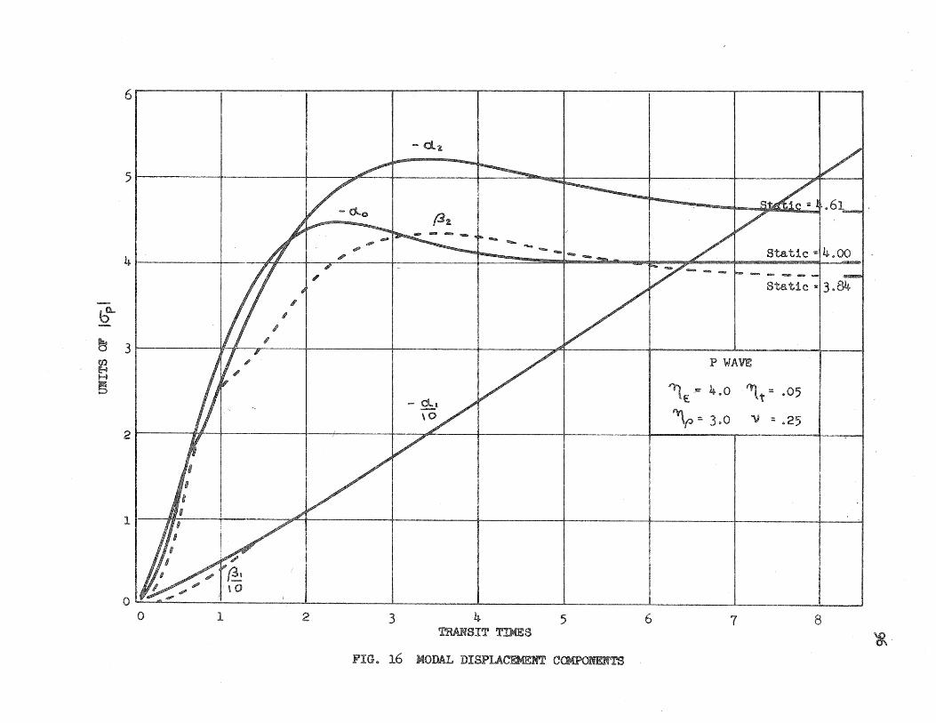
6
- d. a
51 ~ ~ ~
(32.
4 1------4------...... -""'"
~
~ 31
~ H
~
P WAVE
~ES= 4 ,,0 ~t::: ,,05
"\p =. 3GO v:: e25 2
1
O~~----~~----~-~L---------L---______ ~ _________ L-________ L-________ L-________ L-__ ~
o 1 2 3 4 TRANSIT TIMES
5
FIG .. 16 MOnAL DISPLACEMENT C<J4PONEBTS
6 7 8 '&-

5
- <Jeeo
/ ()es'l
Static 1= 1 wo8
3' , P WAVE
: 21 /IfJ 1 L--Ll 1 ~;~::: I :~::: 1
H
§
I
1 \1 -+-- ~ !
(ft.\)1.
~~ 1= 0 ..
o / (f~bo Static I'" 0 .. 10
1 2 4 TRANSIT TIMES
6 7 ~l'~O----~----~----~----~----~--~~--~----~~
3 5 8
FIG.. MODAL COMPONENTS OF SHELL STRESSES
~

~
~ H
~
1.4
1.21 14" ~ 1 -<Tee 1 I. <>h+.J", I
1 .. 0
Static
0.81 I A I I P WAVE
"1£= 4 .. 0 :: .. 05
0.61 U I I ~p = 3.0 V - •25
1 I
o
Static 1= 0 & II
-0 .. o 1 2 3 5 8 9 10
TRANSIT TIMES A"1V~ OF t;.·AAilIJ .... .!!" ... ' .. ·" S~rRE,SSE~S
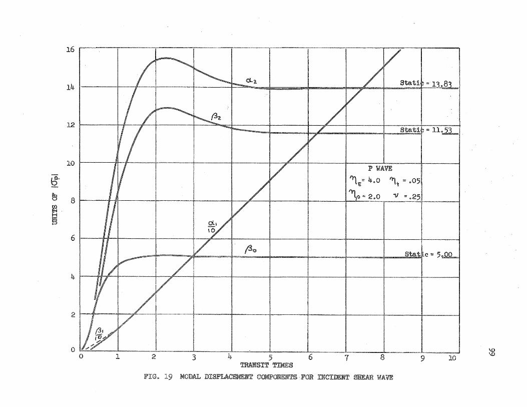
16
14 I-------~_,~_r----~-------~~--~~--~------+_~--~----_+~~~I
12 II-i--
_ 10 I ~ III I P WAVE
~'E= 4 .. 0 ~1:= ,,05
~ 8 I~p= 2 .. 0 11 = .. 25
~ §
6
~
4
2
o o 1 2 3 4 5 6 7 8 9 10
TRABSIT TnmS
FIG .. 19 MODAL INCIDENT SHEAR WAVE
\0 \0

-12
-10
-8
t.;
~ -6
~ §
-4
-2
o
V I
f <reel
II ~
o 1
/~ ~
(f~b2.
2
~ 0-98'2, -
3 4 TRANSIT TIMES
-
5
Static
S WAVE
~e = 4&0 "1t -= .. 05
~p = 2 .. 0 "V = .. 25
Static
--~
6 7
FIG .. 20 MODAL SHELL STRESSES FOR INCIDENT SHEAR WAVE
-9.23 ............
I
-1~
8 8

-12
-10 I k -i
-8
~
i -6,
1
~ ()"b -
-CJ6Is,(45@ )
2 3 4 5 TRANSIT TIMES
6
P WAVE
,~::: 4.0
~(J ::: 3~0
- -+
7
~t ::: &05
V ::: .25
"""'i
........ ..............l~ __
8
FIG" 21 HOOP AND BEIrn:mG STRESSES OF THE SHELL AT VARIOUS ANGLES
lr.:d1
o fId

0 .. 6 "
0 .. 5 P WAVE
~~ :: 4.0 '\, = .. 05
0 .. 41 ~f' = 3.0 1) = .. 25
I , l:)
~ 0 .. 3
~ H
§ I I
-cryy (45@) 0 .. 2 "
0 .. 1
)
0 .. 0 !be .l\ ' J
o 1 2 3 4 5 6 7 8 TRANSIT TIMES b
ro
22 RADIAL AND SHEAR STRESSES IN THE MEDIUM AT THE BOUNDARY

3 .. 0
2 .. 5
2 .. 0
bo...
~ 1 .. 5 ~ ~
leO
0 .. 5
0,,0
I
" ,
,~ " I'
i- ..... - - ~ '( c) ... - - - - - ~"-.Qe6 ... go (unlined)
,. - - - - - - - ,... - - - .po. - -
.I .
I I
I .1
,. I , _ O8"",(goO)
I / P WAW
I "'l" = 4.0 tilt = .05
/ ~r = 3.0 11 ~ .25
/f ~",- -<f88 .... (45°)
,'V , j~ -
7~ '- -~- --~ l--~ __ -:~~OO)~ _ _. .... __ _ o 1 2 3 4
mABSIT TIMES 5 6
23 HOOP STRESSES llf THE MEDIUM AT THE BOUlmARI
1 8
b w

... 12
/ I;--~
"" ,
/ ~""""" , I ....... ....... (f'smax
I
1'- ____
~ama~G!I!llmlJ ....... ""i"''''''''-- ~ aJ!iD ~ ~ .............. ..,# IJI"'" /~ /'
I I----[7
I <Jees(45@) Oih ~
... 10
l \
I I
0'
e -6
V S WAVE ;
I E = 4 .. 0 m .. 05
/J ~f> == 2 .. 0 V = .. 25 -' I
-8
I I
I "" _'" """"e _ .. _
I '" ~~.~.~ a." 088-145.°1 (unlined) ",'" - ... -............ ""
~ 6i
/ (f1
;' -4
'/ ,e~(4.5@) /
ill
.I
,;/ )
-2
I
o o 1 2 (I, 3 4. 5 6 7 '8 \ b
~~..l'JJ.' TIMES ~
IN THE SHELL AND FOR IJiClDElfT SHEAR liA VE

-12 P WAVE
'Ja'" 4.0
-10 r- i I _ I I "p ~ 3.0 :;JP' ::::: ~, =1
:,,01
11 :: e25
-8
1t = .05 - I \ ~
~ -6 ~ I II ; s10
~
-4
(unlined) .. ~ • ~ e ~ ~ So ~ ~ ~ ce t~
-2
o d
o 1
FIG ..
2 3 4 TRANSIT TOO!S
5 6 7
S'TRESSES IN T.BE SHEll. AND MEDIUM FOR VARIOUS RELATIVE THICKNESSES OF SHELL
8 ~,.!l
{)1 '\11!

-10 2
I 0 P WAVE
-1 ..
~E = 4 .. 0
~? = 3.0 11 = v25 -0. tl
b I
~ -0 •
~
o;.y (90°) I'h. L ~ -r---.-... It ": .. 10
. I.,.i , H
~ I
!
-0 .. I uY \" font:!; \ nn. I.
;r
It = .. 05
/ / ~
I I
(;
?/ ~y 19o~J ~t:: .. 01
~ ~
-0"
o ~-----------.--.~-.--- ~-.-
o 6 4 5 TRANSIT TlXES
8 2 1 7 3 b 0\
FIG" 26 RADIAL STRESS IN THE MEDIUM AT THE BOO!IDARY FOR n.u.ll.VVU THICKNESSES OF SHELL
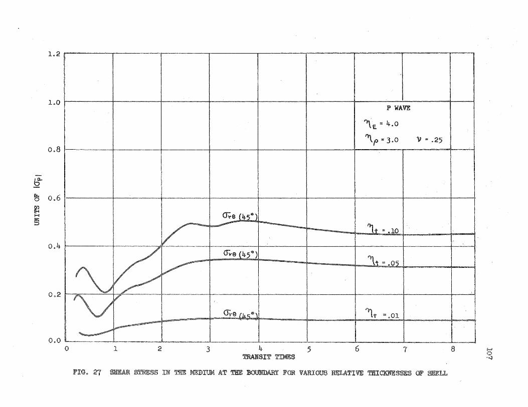
le2
1 .. 0
008
~
~ 0 .. 6
~ H
E§
0.4
0 .. 2
0,,0 o
Cf;e (45") --/
i""""""
~ Che{45°)
~ V-
V /'
0';.9 fhc.° \
~ ~---
1 2 3 4 5 _VU'3SIT TDlES
SHEAR IN THE AT THE BOUNDARY 'OR VARIOUS Ju.~uru
P WAVE
~E. = 4.0
'\p ::: 3.0 11 ,.. .25
~t ::: .10
,'" - ~O5
~t =,,01
6 1
THICKJIESSES OF SHELL
I I
,J
8 il-» c> ~

1.2 _ I
I
I I I i I !
0.8 ~ t-------t--------r--.. ---I I '
! .
0.4
~
~ 0 i -,..,
~ ~
I I
I I
-0 .. 81----- ~'-I
I I I I !
i I I
-1 .. 2 I I I ________ 1 ___ I 1 2 3
RADIUS R 4 5R
-2.4nl'-------;--------~------~--------
... 2 $ 0 1--.-----.. -- .-... -._+ .... --_._ ...... _--.-.-
\
\ \
P WAVE
"E ::: 4.0
I f = 2 .. 0
It = .05
11 = .. 25
-1 .. 6 1--\----+---·-------· .. +------ -'1"""' ------,-____ --l i ~ \
\ \ ; I)
\GSa i (90 )
" -1 .. 2 r--.-.----... - .. ---~~
i I
-- - unlined cavity
( 0)
I <i;.." 0 '-.--l _ I ... 0.8 1----·- ... ---.- ------.-i--------~-.:.+...e..~-------._t_
"
-0 .. 4
I I
o.otL- I I 1 2 3
RADIUS R 4 5R ......
o co
FIG II> 28 STRESSES IN THE MEDIUM FOR VARIOUS RADII AT TEN TRANSIT TIME
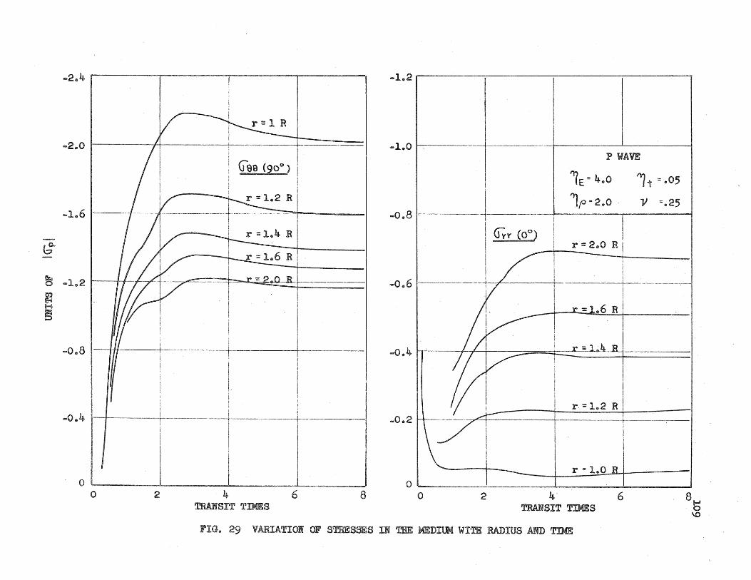
... 2.4
... 2.0 I A -=r:r======:::::==
",,1<116
-<S
~ o -1.2 to E-G H §
... 0.8
... 0.4
o o 2 4
TRANSIT TIMES 6 8
-1.2 ,~------------------------~------------------------
P WAVE -1.0 ~ '--l-- 1 = 4.0 It = .05
1 E
! 11 ".25 I ~ t ---- j -- i
I O! I Uvv (0) ! r = 2.0 R I I I I I ~:
I
... 0.8 k·-··----
-0.6 , --'------~- ..........,-------+---.. --~--.-----
-0.4 Ii' I /
-0.2
r:c 1.0
o .. --________ ~ ________ ~~----~~----------o 2 4' 6 8
TRANSIT TD4ES ~
FIG. 29 VARIATION OF STRESSES IN THE MEDIUM WITH RADIUS AND TIME

~
~
~ H
~
4.0r-. -----r--
3.2 S WAVE
1 E:: 4.0 '1 t = .. 05
'1 f ::: 3.0 V = .. 25
- Uael I .,
! I L __ _ -----+-----.- i --~
GYe;zi - , I
: i I 0.81 ----r----~·~~I ::::::::=:==1
~ I I
Orr 7"
!
I -0 .. 81 at ten transit time
I
1 .. 0 2 .. 0 3.0 RADIUS, R
4.0 5.0
4.0
I I
3.2 I' -----4----J ! I
e ll i - . I i
. .! : -.....r_.= __ l;..;;..O..;;......;;;.R~I ____ ,
2.41 I ~ I ; -. i I - cree (45) ! I
.....;;;...;;0. __ ·1 I
r -= 1 .. 2 R I i f I
1 .. 6 I I / +
0 .. 8
o I " 'v" Gyy (0°)
! !
~-- ---------.!
r:: 2 .. 0 R
r :: 1.0 R
-Oe8 L' ________ -L ________ ~ ________ ~ ________ ~
o 2 4. 6 8 TRANSIT TIMES .....
b FIG. 30 STRESSES IN THE MEDIUM FOR VARIOUS RADII AND TIMES

.24,' ----~----~----~------~--~ .. 24,' ----~---'-------r----------r------,-------
.. 161 .....
Ul E=I ~ o12[
81 _ II
A ~ H
~ .. 08 0 H ro
I ~ .. 04 ~ 0 z
- .. 04
o
- Machine Sol ..
-- - Short Time Sol.
P WAVE
"e = 4.0 1t = .. 05
..161 \ ,'p = 2 .. 0 i "'II:: .2, I
1 p'''(n • l~ .j \J I~ - F (n:: 21)
1/80 2/80 , 3/80 4/80 5/80 0 1/80 2/80 3/80 TRANSIT TIMES
FIG.. 31 COMPARISON OF SHORT-TDm. RESULTS FOR INCIDENT P WAVE
4/80 i-'
5/80 l:!

1.6 le6
I I
1.41
I P WAVE 1 .. 4 I
.......... Machine Sol .. '1E = 4 .. 0 't =,.05
1--Short r
TimeSo1
'1 J
1.21 11,., = 2.0 1.2 I
---.~ I I ~-- -r= --T- 1.0 H 1.0 ~ A ~ H
~ 0.8 I Y 'L // 0.8:
H
! @ 0 .. 6 I I
I +- zi , J 0 .. 6 ~ ~
0 .. 4
Oe2 If I "'" o. 21 '1/ -1--------1
0,,0 ...........-: I I I I
o 1/80 2/80 3/80 4/80 5/80 0 1/80 2/80 3/80 4/80 5/80 ~ TRANSIT TDIES N
3~~ COMPARISON OF SHORT -TIME RESULTS FOR INCIDENT P WAVE

1.6 1 .. 6
1 .. 4 - Machine Sol.
1.2
- - Short Time Sol.
1 .. ~ P WAVE
'?E= 4 .. 0 I t =, .. 05 /
'f»= 2,,0 ·V = .. 25 I~
2 I ..
f1l ~ 1 .. 01 8 1 .. I 0 § A ~ H
~ 0 .. 81- I I 0 .. §
0 8
H W
S A 0,,61 / :1'1 0 .. D
~ 6
~
0 .. 41 tI' 1/ o. 4
0 .. 2 1 1 /' Y ;/ 0 ..
0 .. 0, ~ -d=:::::=: 1 1 I 0 .. 0 o 1/80 2/80 3/80 4/80 5/80 0
TRANSIT TDtES 1/80 5/80 ~ w 2/80 3/80 4/80
33 COMPARISON or SHORT-TIME RESULTS FOR INCIDENT P WAVE

lo2ri----------~----------r----------.----------~--------~ 102
1.01 ·1
1.0
1 I S WAVE
--Machine Sol. 'E = 4.0 1t:: .05
0.81 _. -Short Tiae Sol. I I i 0.8 1 I 'f= 2.0 ·11 =.25
~ 0.61\ ~
0.6
~
~ 0.4 H
I • 0.2
~ ~
",
I-F (n = 1)
0(00 ------
.... 0 .. 21 7' ... ........ ........
-0 .. 4 ft iii I I -01& 4. ! ! i i
o 1/80 2/80 3/80 4/80 5/80 0 . 1/80 2/80 3/80 4/80 5/80 S TRANSIT TIMES
FIG .. 34 COMPARISON OF SHORT-TIME RESULTS FOR INCIDENT S WAVE

ttl E-4
§ ~
~ H w
I g
~ z
3.2
I ./
./ 2.81 /~ ~
2.41 Y (' I
2 .. 0 ............ Machine Sol ..
- - Short Time 801<11
1e6 .. /?:;c
l
----i 1.2~~-+--
''\ I
+-~ 0.81 I / I" I
0.4111 - -g ::A""""-:
3 .. 2
2.81L-~---+------+-----~------~----~
2.41 / '........j
2 .. 0
le6l-L S WAVE
''E= 4.0 1t= e05
_1f= 2 .. 0 11 = .. 2;
1.2
0 .. 8
0 .. 41' ~r ...... "'"
0.,0' ====! I I I 0",0..........-= ! I ! ! I ...., o 1/80 2/80 3/80 4/80 5/80 0 1/80 2/80 3/80 4/80 5/80 ~
TRANSIT TIMES
35 COMPARISON OF SHORT-TIME RESULTS FOR INCIDENT S WAVE
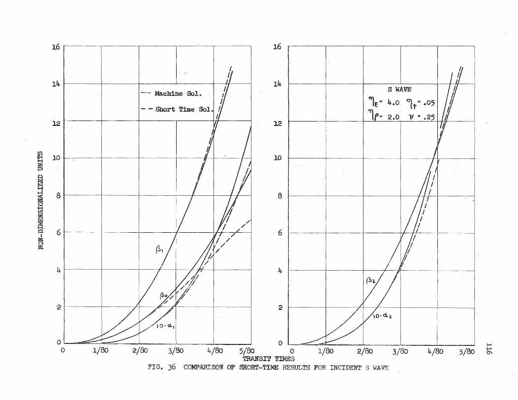
16 16
lq.1 I I - Machine Sol. I ,1 lq. I I S WAVE
'1e= 4.0 1t = .05
1f= 2.0 121 ~l 12
~ 10 l-, H I I 10 H ,
§ A
~ ~ 81 f.
I f. , I J 8
H tf.)
~ 61 t- -f-----. -+ff--~-j ~ 6 D
~
41 ,
J /11 I 4-
2 i --+ //:#' ~ 2
0 1 ~I~ / 0.""........- = ! ! I ! ~
o 1/80 2/80 3/80 4/80 5/80 0 1/80 2/80 3/80 4/80 5/80 th TRANSIT TIMES
rIG. COMPARISON OF mORT-TIME RESULTS FOR INCIDENT :3 WAVE
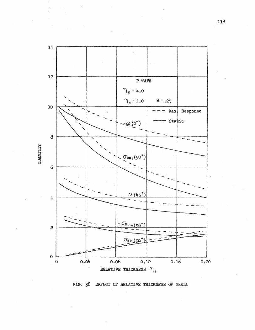
118
14
12 P WAVE
"\E: = 4 .. 0 ....
.... ~f:;: 3 .. 0 v:= .. 25 ..... 10 .....
..... Max Response ..... ...... .....
--~ (0°) Sta. ic
.......
-8 -- -- .... -i::
~ Of
6
--..... ,
4 - - -
o ----------~--------~--------~--------~---=----~ o 0.04 0 .. 08 0 .. 12 0 .. 16 ·0.20
RELATIVE THICKNESS ~t
FIG. 38 EFFECT OF RELATIVE THICKNESS OF SHELL

119
10 ~------~~~~~-4--------~--~-----+--------~
I I
8 ~------~~~-----4~/~/~~--+---------~------~ P WAVE
I
t -= .05
~p == 3.0 \J = .25 6
- - - Max Response
- Sta ic
4.
2
o ~~----~--------~----~--~--------~~------~ o 4 8 12 16 20
RATIO OF MODULI OF ELASTICITY ~E
FIG. 39 EFFECT OF RATIO OF MODULI OF ELASTICITY

120
14
- - -Max n "£"
- Sta 6>lc 12
P liA-VE
:: ®O ::: .,05
\) ':. ..
- d.(o@l = - F ~ ~ - -
t - .... --.- - - - --- - ------
10
..- - - ---- 9s(90_@»_ ..- ---!--- ..-- ~ - ...... - -8
6
!:J -- """" --.i- ~ - -- ~ ~ ~ ..... .-~ - ... - - ..... ~
------f
- __ J - -- ~~ ~ - - - -.... .... - - - - - - -"" - .-
2
I .. - -!-o -- ""'" - - - ,.., - - j2Q'~jl- - - - - - F- - - - -.,
o I I
o 4 6 8 10
EFFECT M.liSS RATIO

121
12 P WAVE
" " " '\ 10
8 ,-d...(00)
~ , H \
~ Of 6
o b-~ __ ~ __ ~ ________ ~ ____ ~~~
o 0 .. 2 0.,4
POISSON'S RATIO \)
FIG.. 41 EFFECT OF POISSON g S RATIO
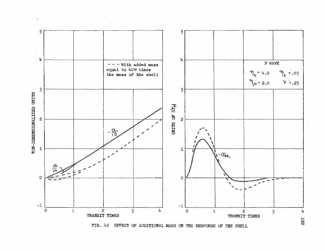
~ § A ~
~ 0 H to ~
~ ~
a
~ ~
5 5
41 4 , - - - 'With added mass equal to 40". times the mass of the shell
3 3
(-j
2 ~ 2
~ d... .. H
§ --• n
Ii /1 , 1
o o
-1 b-____ ~~ ________ ~ ________ ~ ______ ~ -1 o 1 2 3 o
TRANSIT TIMES
P WAVE
~E = 4 .. 0 ~t =" .. 05
~p == 2 .. 0 V ~ .. 25'
, .... '\
I \
,~ I \ I '\ I \
~ 1
,~
~-"" '\ " "
, ..... - ~"
2 TRANSIT TIMES
3
- "'""
FIG .. 42 EFFECT OF ADDITIONAL MASS ON 'mE RESPONSE OF THE SHELL
4 ~
~
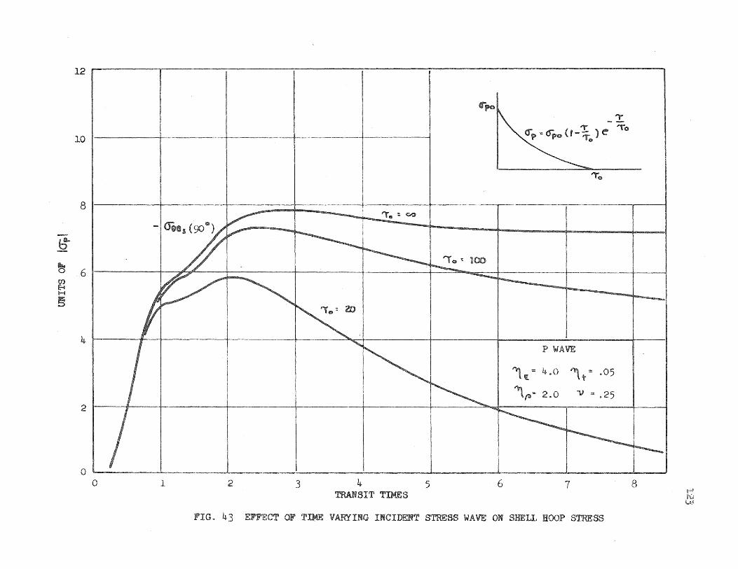
~
~
~ H
§
12
10 ----+-1 .. - .. -------.... ···+--.. ---·-·-.. -·---+-·· .. ------·-·-·--·-t----!
i I -----+---
"l'1\J :. c..o 8 I r- ~-l--..."""-..._L
G"'po ..,.. <Tp ,. <f"po (t - '!'. ) e- 1"'0
'To
""0
6 I :#. -+- +.-----.......:::::l'e ...... iiIii!ii!iii:::""""':---t-----
4 » ,
P WAVE
E 4~o ~t =: .05
2 I f t _ -+ + ~ "\f>~ 2.0 v· .25
o L~ __________ ~ __________ ~ __________ ~ __________ ~ __________ ~ __________ l __________ =_~ ________ ~ ____ _J
0 1. 2 3 4 5 6 7 8 TRANSIT TIMES
FIG" 43 EFFECT OF TIl(E VARYING INCIDENT STRESS WAVE ON SHELL HOOP STRESS

~ H
!5
12 Up
o;@
101 ---j
"0 -OQ9~ (90@)
8~1 -------~------~------~------~-------~-------r------_r------_r---
61-1 -~---+-
41---P WAVE
~E. == 4 .. 0 ~t "'" ,,05
~p= 2 .. 0 V = ,,25
2 --I-+---.----l--------t--~----.....".-------+_------+_
Om -" o 1 :2 3 4 5 6 7
..II.J!.VU'llU'.A.A TIMES
44 EFFECT OF TIME ON SHELL HOOP STRESS
8
~ ~
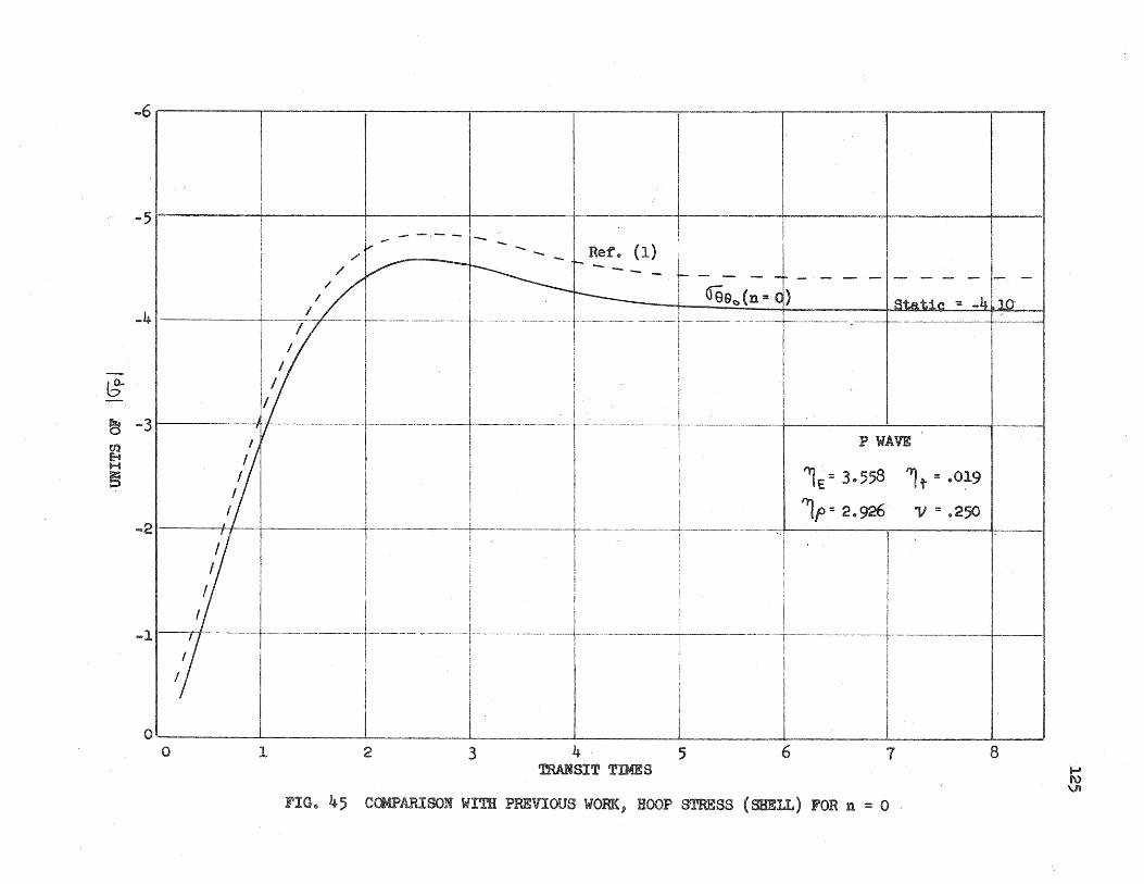
-6~1----------'-----·------~---------'-----------'----------.----------'r----------.----------.-----,
... 5 i
;L' ,I
I I i --+.--' I + _____ ~__ .1 i -----+--- i - - 1: -I (/ -r-u
-------- t --- -- ._--j----- ----1- ~9~ (~=t-- I staUc - ) 10
I
I I Iii --- ~~ I Ii! 1
1/ I : I I I !
. -------1--- I I· ! --------I" --.------- -t-----------+----------.-.. I :
I I : 't) .
... 21 /1 t -----4----------L-~---- I I. IE: 3.558 "It = .019 ! I !, +---.. -------t--------- 1f 2 .. 926 V = .250 i I ; --I-cr' ---"------r-----=--J
1 I I ! I . !
I i I I
I I I I Ii: ----f---- I i: I I ! I
I ~--,- --- _L_ 'i~_
I
I ! --------- --t--- ---.. -----~------- ! t-: i I : -- !---~-~-- -----i I ,-------- ---.-
I I I I I ! I
0 1 I _______ I L I I I I - - I I I I 6 I
7 8
~
~ -3
~ H
§
-41--
-1
o
I -,- 1-- --
P WAVE
1 2 4 5 3 TRANSIT TIMES
45 C()fPARlSON WITH PREVIOUS WORK, HOOP STRESS (SHELL) rOR n = 0
...., ro VI
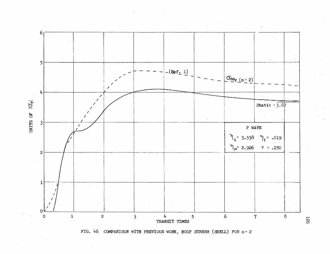
6
5
4
b ~ ~ 3 H
~
2
1
o o 1
--------- <rSB2J.n.:.~, L ~
------r ~E= 3.558 1t =
~p= 2 .. 926 I
I
I
2 3 4 5 6 1 TRANSIT TIMES
FIG.. 46 COMPARISON WITH PREVIOUS WORK, HOOP STRESS (SHELL) FOR n = 2
-8 f-'
I\) 0'\

~--r--r---r-~II-r--' -6 I
I _I
!
! 1
-5
I - - - Rei'. (1) I I - - 1 I -;-.--- +----+-
i -' {n:: O~ - """"0 I
/ /
-1- - - - j_ I
Static :: -4 .. 10
~ -41----------[--7 Q
~ i! ~ ! I ! I f:il'.Go - -3 ---------------------\--! I I ~ / I I ----1---------1~------ r-j --_-P-W....!-AVE---~--
~ I I I I 1'1: - 3. 558 -'\-I- =. 019
~ -2 I -t' -----------i-----------------------t_!-----------l-.--------------------1'------- _ 'l~= 2 .. 926 V = .. 250 _ I I ' _-------11 ------.--------1----
I, \ j ! i - I I '
,I i I I I I ' I I : I Ii i I ! i I I - : I f---..-t --r-----r-----··--1---- -----r----------l I I I I I I
I I I I
-1
o o 1 2 3 4 5 6 7 8
TRANSIT TIKES
41 COMPARISON WITH PREVIOUS WORK, RADIAL DISPLACEMENT FOR n :: 0
..... ro ~

-61 I I I ' I
-51 +--- / .0 -I c- - - *~ ~ J I I I ." I ==1 - - _ I i
I r/ I d.' I --+----t!
II I / I len :: 2) ! i ' - - - -I' I" i ----r-. --:==-=~
4 ~-'---'--_-_'_TI ---.-.-~.-- I . ------L--~ S~t~_c _d ~~~ ---L ~""I I !!,' -1---
~ I i I ! I I I ~ I I / I I I I J" H I 1/ I I I I I, ~ -31-----y- I I -r-----I p W~VE - .
! I i I I i
I I I I 'Wl
~ -2~~i 1---- I ---t---'-t-----} .. If"" 2.926
1
V =.250
I I I I !, I " I, ! I! ill I
-+-- .---~.----- t-------i------t- ·t-----i--,-~---t-----t II I I' I I I I I I l "I' I 0---- I I I _. ___ ~ _______ l_.__ I
o 1 2 3 4 5 6 7 8 TRANSIT TIMES
I-'
~
48 COMPARISON WITH PREVIOUS WORK, RADJl:AL DISPLACEMENT FOR n -= 2

6,
51 -t----- _---- _ -I I I I ./ - - - - - -J (Ret e 1) I
" ,/ ,/ [- ---------1- ----1- --~I ~(~~ I
~§ -------l- IStatic = 3-96 I Iii
J J
- / I I ~ I I
~ 3 -- -t--~ I p~ til i = 3-558 t=
~ ~ 2 ---t-. "tp: 29926 V ~$250 ~I ~
I I
1 I I I L_J I
1 +---~-1--- --+-----l--
I I I I
o -_-L-_L L "----'--I __ --L.
o 1 2 ~~ 4 5 6 1 8 ..., ro \0 iRM'SIT TIMES
WORK, TANGENTIAL FORD: 2

Distribution List for Technical Heports Issued Under
Contract Nonr 1834( 03), Project NR.-064=183
Argonne National Laboratory Bailey and Bluff Lamont, Illinois
Armed Forces Special I'leapons Project Po 00 Box 2610 Washington, Do Co ~}lTN~ Chief, Blast Branch (2)
Chi.ef" "l1eapons Effects Di v 0 (1)
Armed Services Technical (5) Ir~oTInation Agency
Arlington Hall Station Arlington 12, Virginia
Ballistic Research Laboratory Aberdeen Proving Ground Aberdeen, Maryland ATTN~ Dr 0 C 0 ~L Lampson
Battelle Memorial Institute 505 King Avenue ColUllibus J Ohio ATTN~ Ho Co Cross
Chi.ef of Bureau of Aeronauti.cs Navy Department vJashington 25, DoC 0
ATTN ~ DK~,22 (l) DE~'23, 'E~Mo Ryan (1) TD=,41, Techo Libo (1)
Chief, Bureau of Ordnance Navy Department Washington 25, Do Co ATTN ~ AD=3,w Technical Library
Chief, Bureau of Ships Navy Department 1vashington 25, Doe, ATTN~ Code 421 ( ,;
Code 423 (1) Code 430 (1) Code 442 (1) Code 449 (1) Director of Research (2)
Chief'} Bureau of Yards and Docks Navy De];lartment Hashington .' Doe 0
ATTN~ Code C=313 (1) Cod,e P=314 (1)
Chi.ef of Engi.neers Engineering Division Military Construction Washington 25, Do Co ATTN ~ ENGEB ( 2
Chief of Naval Research Department of the Navy Washington 25., DoG 0
ATTN~ Code 423 (1) Code 432 (1) Code 438 (4)
Chief of Staff' Department of the Army R.esearch and Divo \vashi.ngton 25.1 D 0 Co ATTN~ ChIef of Research
and Development
Chief.~ Structures Division (2) Research Directorate Air Force Special Center Kirtland Air }."'orce Base ~ New Mexico
Commander Uo So Naval Ordnance Test Station Inyokern., China Lake J Cal1.fornia NrTN~ Code 501
C omrm::t.rl.de r Uo So Naval Ordnance Test Station Pasadena Annex: 3202 Eo Foothill Boulevard Pasadena 8, California AT~~~ Code p808?
Commander 1]0 So Naval Proving Grounds Dahlgren, Virginia

Forest Products Laboratory Madison, ~'risconsin ATTN ~ L 0 J 0 Markvvard t
Library, Engineering Foundation 29 West 39th street Nelv York, New York
National Aeronautics and Space Admin~istration
Cleve1an(1 Municipal Airport Cleveland, Ohio ATTN~ Jo Ho Collins, Jr.
Nati.ona1 Aeronautics and Space AdminiE',ration
1512 H st~eet, N.W. Washington 25, Do C.
National Aeronautics and Space Administration
Langley Field, Virginia ATTN~ Dynamic Loads Branch (1)
Structures Lab (1)
Naval Air Experimental Station Naval Air Material Center Naval Base Philadelphia 12, Pennsylvania ATTN~ Head, Aeronautical
Materials Laboratory
Naval Ordnance Laboratory White Oak, Maryland RFD 1, Silver Spring, Maryland ATrN~ Mechanics Division (2)
Naval Ordnance Test Inyokern, China Lake, California ATTN~ Scientific Officer
Office of Air Research ~'lright=Patterson Air Force Base Dayton, Ohio ATTN~ Chief, Applied Mechanics Group
Office of the Chief of Engineers Assistant Chief for Public Works Department of the A~y Bldg 0 T=7, Gravelly Point' Washipgton 25, DoC 0
ATTN~ Structural Branch, RoL. Bloor
=3=
Office of Naval. Research (2) The John Crerar Library Building lOth Floor, 86 Eo Randolph Street Chicago 1, Illinois
Office of Chief of Ordnance Research and Development Service Department of the Army The Pentagon Washington 25, Do Co ATTN; ORDTE (2)
Officer in Charge Naval Civil Engineering Research
and Evaluation Laboratory Naval Station Port Hueneme;) California
Officer in Charge Office of Naval Research Branch Office) London Navy Noo 100 FPO, New York, Ne,v York
RAND Corporation Nuclear Energy Division 1700 Main street Santa Monica, Californi.a
Research and Development Board Department of Defense Pentagon Building ~'lashington 25, Doe. ATTN ~ Library, Code 3D-=1075
Superintendent Naval Gun FJactory Washi.ngton 25, Doe 0
Superintendent Post Graclua te School Uo So Naval Academy Monterey, California
DoS. Atomic Energy COrD11li,ssion Division of Research Washington, Doe 0
Do So Coast Guard 1300 Eo Street, NoWo Washington, Do Co ATT.N~ Chi.ef, Testing and
Development Di. vi.s ion

Profo Mo Gensamer Department of }1etallurgy Columbia U~iversity NevT York) NevT York
Dr. Martin Goland Vice President Southwest Research Insto 8500 Culebra Road San Antonio, Texas
Dr. J. No Goodier School of Engineering Stanford University Stanford) California
Proi' 0 :La Eo Goodman Dept 0 of Mechanics and Materials University of Minnesota Minneapolis, Minnesota
Prof 0 Ao Eo Green Kings College Newcastle on Tyne 1) England
Dr 0 Ro JoHansen Massachusetts Inst. of Technology Cambridge 39, Mass.
Prof 0 Ro Po Harrington, Head Department of Aeronautic Engo University: of Cincinnati Cincinnati 21, Ohio
Prof 0 R. Me Hermes Uni vers i ty of Santa Clara Santa Clara, California
Prof 0 No 30 Hoff, Head DiVa of Aeronautical Engineering Stanford University Stanford) California
Dro H 0 Ho Hoppmann Department of Mechanics Rensselaer Polytechnic Institute Troy, New York
Prof 0 Lo So Jacobsen Stanford University Stanford, California
=5~
Dro Bruce Johnston 301 We Engineering Building University of Michigan Ann Arbor, Michigan
Prof 0 \'10 K 0 Krefeld College of Engineering Columbia University Ne"\v York, New York
Dr. Ro Latter RAND Corporation Nuclear Energy Division 1700 Main sto Santa Monica, California
Profo Bo Jo Lazan Department of Mechanics University of Minnesota Minneapolis 14, Minnesota
Prof 0 George Lee Department of Mechanics Rensselaer Polytechnic Institute Troy, New York
Dro Me Mo Lemcoe Atomics International Canoga Park, Cali.forni.a
Dr. Co Wo MacGregor Engineering Buildi.ng Dni versi,ty of Pennsylvania Philadelphia l~, Fa 0
Prof. Ro Fo Mehl Metals Research Laboratory Carnegie Institute of Technology Pittsburgh, Pac
Dr. Me Lo Merritt Sandia Corporation Sandia Base Albuquerque, Ne,,·j Mexico
Prof 0 Jesse Ormondroyd University of Michigan Ann Arbor, Michigan
Prof 0 H 0 R 0 Osgood Department of Civil Engineering The Catholic Uni versi.ty of America Washington 17, D. Co


![Critical ideals of graphs - CINVESTAV · G], the determinantal ideals of L(G;X G) are ideals on Z[X G] which we call critical ideals of G. Next we study how the critical ideals encode](https://img.pdfslide.us/doc/110x75/5fa3f5e4efc6f36b113a3fab/critical-ideals-of-graphs-cinvestav-g-the-determinantal-ideals-of-lgx-g-are.jpg)


![Polynomial Ideals Euclidean algorithm Multiplicity of roots Ideals in F[x]](https://img.pdfslide.us/doc/110x75/56649cf45503460f949c2c78/polynomial-ideals-euclidean-algorithm-multiplicity-of-roots-ideals-in-fx.jpg)