Embed Size (px)
Citation preview
Identifying the Urban Poor in Brazil
James F. HicksDavid Michael Vetter
WORLD BANK STAFF WORKING PAPERSNumber 565
20
K,,
...
Pub
lic D
iscl
osur
e A
utho
rized
Pub
lic D
iscl
osur
e A
utho
rized
Pub
lic D
iscl
osur
e A
utho
rized
Pub
lic D
iscl
osur
e A
utho
rized
Pub
lic D
iscl
osur
e A
utho
rized
Pub
lic D
iscl
osur
e A
utho
rized
Pub
lic D
iscl
osur
e A
utho
rized
Pub
lic D
iscl
osur
e A
utho
rized
WORLD BANK STAFF WORKING PAPERSNumber 565
Identifying the Urban Poor in Brazil
James F. HicksDavid Michael Vetter
The World BankWashington, D.C., U.S.A.
Copyright © 1983The International Bank for Reconstructionand Development / THE WORLD BANK1818 H Street, N.W.Washington, D.C. 20433, U.S.A.
First printing April 1983All rights reservedManufactured in the United States of America
This is a working document published irnformally by the World Bank. Topresent the results of research with the least possible delay, the typescript hasnot been prepared in accordance with the procedures appropriate to formalprinted texts, and the World Bank accepts no responsibility for errors. Thepublication is supplied at a token charge to defray part of the cost ofmanufacture and distribution.
The views and interpretations in this document are those of the author(s) andshould not be attributed to the World Bank, to its affiliated organizations, or toany individual acting on their behalf. Any maps used have been preparedsolely for the convenience of the readers; the denominations used and theboundaries shown do not imply, on the part ot the Wrorld Bank and its affiliates,any judgment on the legal status of any territory or any endorsement oracceptance of such boundaries.
The full range of World Bank publications is described in the Catalog of WorldBank Publications; the continuing research program of the Bank is outlined inWorld Bank Research Program: Abstracts of Current Studies. Both booklets areupdated annually; the most recent edition of each is available without chargefrom the Publications Distribution Unit of the Bank in Washington or from theEuropean Office of the Bank, 66, avenue d'Iena, 75116 Paris, France.
James F. Hicks is senior public finance specialist at the Research TriangleInstitute and David Michael Vetter a statistician with the Instituto Brasileiro deGeografia e Estatistica; both are consultants to the World Bank.
Library of Congress Cataloging in Publication Data
Hicks, James F., 1944-Identifying the urban poor in Brazil.
(World Bank staff iorking papers ; no. 565)Bibliography: p.1. Urban poor--Brazil. I. Vetter, David Michael,
1943- . II. title. III. Series.HCl90.P6B52 1983 339.4'6'0287 83-6912ISBN 0-8213-0177-2
ABSTRACT
Brazilts urban poverty target group is defined by the World Bankby using the concept of relative poverty, in which the poverty line isestimated as one third the national per capita income, adjusted forurban-rural price differences. It is common in Brazil to transform cur-rent cruzeiros into minimum salary units. The minimum salary is alsodetermined on a regional basis; currently there are three regional mini-mum salaries.
The Bank has used a national, urban poverty line mea.sured in unitsof the highest regional minimum salary. Recent appraisals of urbanprojects have used three regional minimum salaries for all regions asthe relative poverty line. In using a single urban poverty line, theBank implicitly assumes that regional differences in the cost of livingare accurately reflected by the regionally differentiated minimum salaries.
The basic objective of this paper is to investigate the degree towhich the use of a single urban poverty threshold in Brazil may lead tobiased project identification, design, and evaluation. Absolute povertylines are defined by the use of estimates of expenditures for minimum-cost, nutritionally adequate diets and food shares of total expendituresby families with incomes roughly equivalent to the Bank's relativepoverty standard. This approach permits estimation of city-specific,minimum-diet food costs and poverty lines in 25 cities and analysis ofthese estimates over time, as well as between and within regions.
The average, per capita cruzeiro cost of the food basket was foundto be highest in the poorer regions. Because regional minimum se ariesare lowest in the poorer regions, this result raises questions about theBank ts current standard of using a single relative poverty, line. Thestudy concludes that converting the national poverty line expressed incruzeiros to minimum salaries expressed in the regional values woulddecrease the risks of bias in urban project design and appraisal.
ACKNOWLEDGEMENTS
We wish to acknowledge a special debt of gratitude to Mr. Peter
Watson. The need for this type of research was identified during urban
project appraisal missions in which we participated. Mr. Watson also
served as project sipervisor and made many useful written and verbal
contributions to our effort. Illis insights were particularly useful in
helping us to direct our study as closely as possible to the needs of
the Bank's urban projects staff. Mr. Watson's secretary, Ms. Lelia
Hedrick, was also quite helpful in providing and processing information.
The collaboration of Mr. Gregory Ingram was especially important
and useful at the initial stages of this study. He met with us in Rio
de Janeiro and made many helpful suggestions for our methodology. He
also gave us written comments in the Draft Version of this study which
have substantially contributed to this Final Report.
Ms. Louis Fox and MIr. Fred D. Levy also provided us with written
comments on the Draft Version, and Mr. Vinod Thomas, verbal ones. We
appreciate their interest and useful suggestions.
None of these people has reviewed this Final Report, and none is
responsible for any errors in data gathering and analysis, or in the
conclusions and recommendations presented here.
TABLE OF CONTENTS
Page
ACKNOWLEDGEMENTS
I. INTRODUCTION AND SUNMARY OF MAIN FINDINGS 1
2. GENERAL METHODOLOGICAL CONSIDERATIONS 4
2.1 Overview 4
2.2 The Unit of Analysis 9
2.3 The Instruments of Measurement 10
2.3.1 Regional Minimum Salaries 10
2.3.2 National Household Expenditure 13
Survey - ENDEF
2.3.3 National Price Survey - INP 15
2.3.4 GetuXio Vargas Foundation 16
3. DEFINITION OF THE POVERTY LINE FOOD BASKET 18
4. ESTIMATES AND ANALYSIS OF THE ABSOLUTE POVERTY LINES 25
4.1 Absolute Poverty Line Estimates Based on 25
Minimum Diet Costs
4.2 Intertemporal Changes in the Poverty Lines 28
4.3 Comparison of Poverty Lines by City Size 34
4.4 Regional Comparisons of the Poverty Lines 34
5. COMPARISON OF ABSOLUTE AND RELATIVE POVERTY LINES 40
AND EVALUATION OF RESULTS
BIBLIOGRAPHY 50
ANNEX I - 1979 Estimates of Urban Poverty Lines 52
in Brazil According to-World Bank Guidelines
ANNEX II - Poverty Line Food Basket 55
ANNEX III - Size Distribution of Family Expenditures 60
by ENDEF Region
TABLE OF CONTENTS
Page
ANNEX IV - Sensitivity Tests for the Absolute 76Poverty Line Estimates
IV.1 - Use of Average Family 76Size Data
IV.2 - Use of Monetary versus Non- 79Monetary Data
IV.3 - Use of Behavioral Diet in 79Poverty Line Estimates
LIST OF TABLES
Page
1. Changes in the Minimum Salary in-Three Cities 12
2. Minimum S.laries for the Surveyed Cities in 1974 14
and 1980 and Comparison of Changes Over Time
3. Nutritional Quality of Sample Diet and Comparison 19with FGV Staridards
4. Selected Least Cost Nutritionally Adequate Diet 22
5. Food Component Quantities of the Minimum Diet 24
Used in Poverty Line Estimates
6. Cost Estimates of Minimum Diet in the Surveyed Cities 26
7. Poverty Line Estimates in Surveyed Cities 27
8. Linear Regression Models of the Per Capita Poverty Lines 31
Estimated for 1974/75 and 1980
9. Estimates of 1980 Minimum, Per Capita Diet Cost Based on 33Five Staple Item Costs and Staple Share in Total Cost
10. City Size ComparisJns of Poverty Indicators 35
11. Inter and Intraregional Comparisons of Poverty Indicators 36
.12. Indicators of Central Tendency and Dispersion of the 38Per Capita Cost of Minimum Diet and Poverty Lines
13. Regional Estimates of Relative and Absolute Family 42Poverty Lines Measured with Different Units of AccouInt
14. Ratios of Absolute and Relative Family Poverty Lines 43
15. Estimates of Number of Poor Families According to 46Absolute Poverty Criterion - 1980
16. Estimates of Number of Poor Families According to 47Bank's Current Relative Poverty Criterion - 1980
17. Estimates of Number of Poor Families According to 48Recommended Relative Poverty Criterion - 1980
18. Comparison of the Number of Families Considered Poor 49According to the Various Criteria
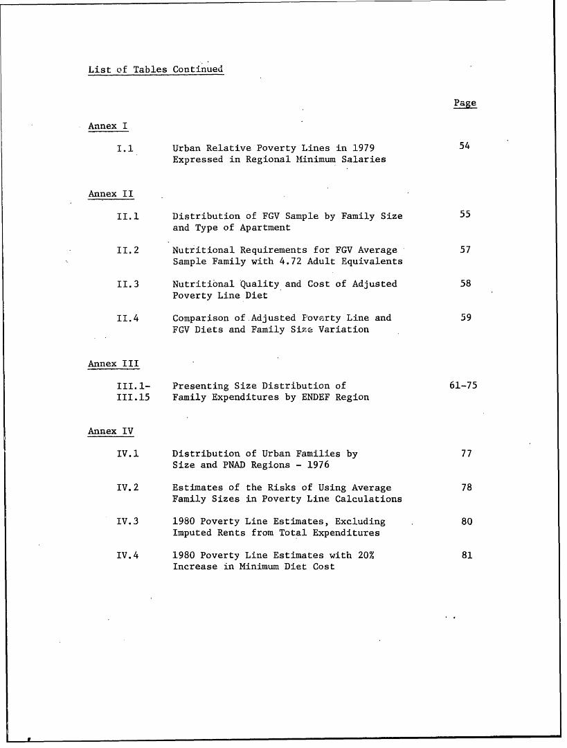
List-of Tables Continued
Page
Annex I
I.1 Urban Relative Poverty Lines in 1979 54Expressed in Regional MIinimum Salaries
Annex II
II.1 Distribution of FGV Sample by Family Size 55and Type of Apartment
II.2 Nutritional Requirements for FGV Average 57Sample Family with 4.72 Adult Equivalents
II.3 Nutritional Quality and Cost of Adjusted 58Poverty Line Diet
II.4 Comparison of-Adjusted Fovzrty Line and 59FGV Diets and Family Size Variation
Annex III
III.1- Presenting Size Distribution of 61-75III.15 Family Expenditures by ENDEF Region
Annex IV
IV.1 Distribution of Urban Families by 77Size and PNAD Regions - 1976
IV.2 Estimates of the Risks of Using Average 78Family Sizes in Poverty Line Calculations
IV.3 1980 Poverty Line Estimates, Excluding 80Imputed Rents from Total Expenditures
IV.4 1980 Poverty Line Estimates with 20% 81Increase in Minimum Diet Cost
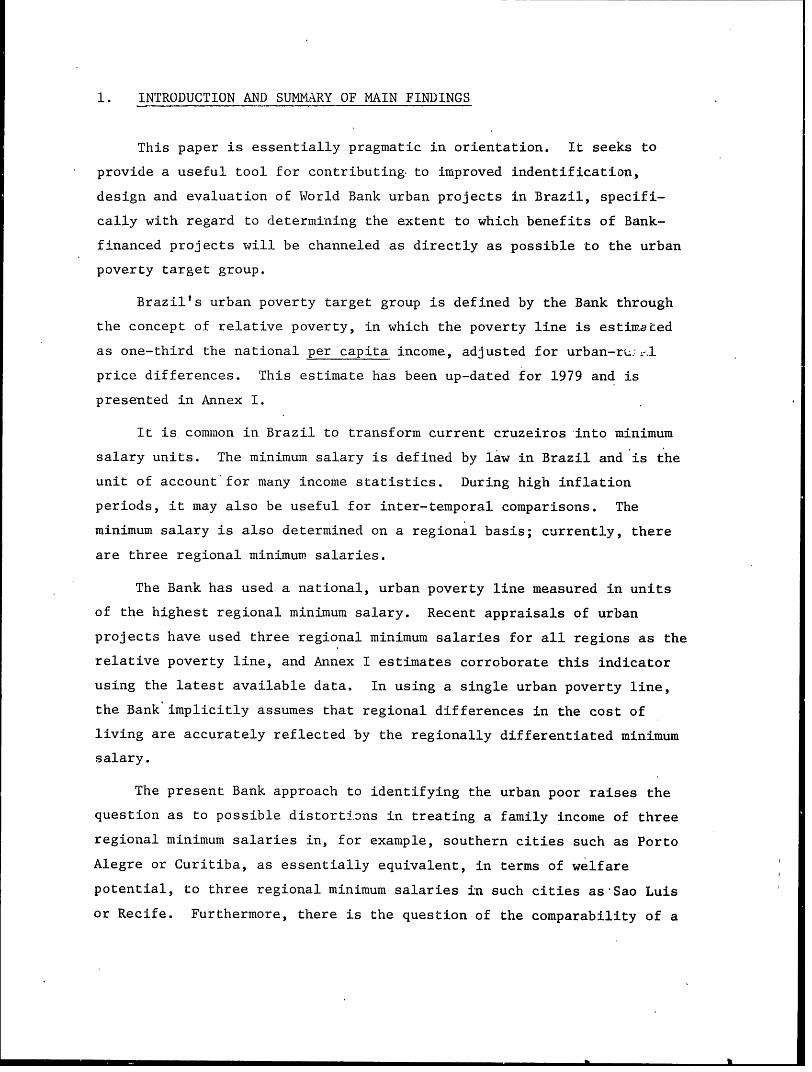
1. INTRODUCTION AND SUMMARY OF MAIN FINDINGS
This paper is essentially pragmatic in orientation. It seeks to
provide a useful tool for contributing to improved indentification,
design and evaluation of World Bank urban projects in Brazil, specifi-
cally with regard to determining the extent to which benefits of Bank-
financed projects will be channeled as directly as possible to the urban
poverty target group.
Brazil's urban poverty target group is defined by the Bank through
the concept of relative poverty, in which the poverty line is estimaced
as one-third the national per capita income, adjusted for urban-rLu-.l
price differences. This estimate has been up-dated for 1979 and is
presented in Annex I.
It is common in Brazil to transform current cruzeiros into minimum
salary units. The minimum salary is defined by law in Brazil and is the
unit of account for.many income statistics. During high inflation
periods, it may also be useful for inter-temporal comparisons. The
minimum salary is also determined on a regional basis; currently, there
are three regional minimum salaries.
The Bank has used a national, urban poverty line measured in units
of the highest regional minimum salary. Recent appraisals of urban
projects have used three regional minimum salaries for all regions as the
relative poverty line, and Annex I estimates corroborate this indicator
using the latest available data. In using a single urban poverty line,
the Bank implicitly assumes that regional differences in the cost of
living are accurately reflected by the regionally differentiated minimum
salary.
The present Bank approach to identifying the urban poor raises the
question as to possible distorti.ons in treating a family income of three
regional minimum salaries in, for example, southern cities such as Porto
Alegre or Curitiba, as essentially equivalent, in terms of welfare
potential, to three regional minimum salaries in such cities as Sao Luis
or Recife. Furthermore, there is the question of the comparability of a
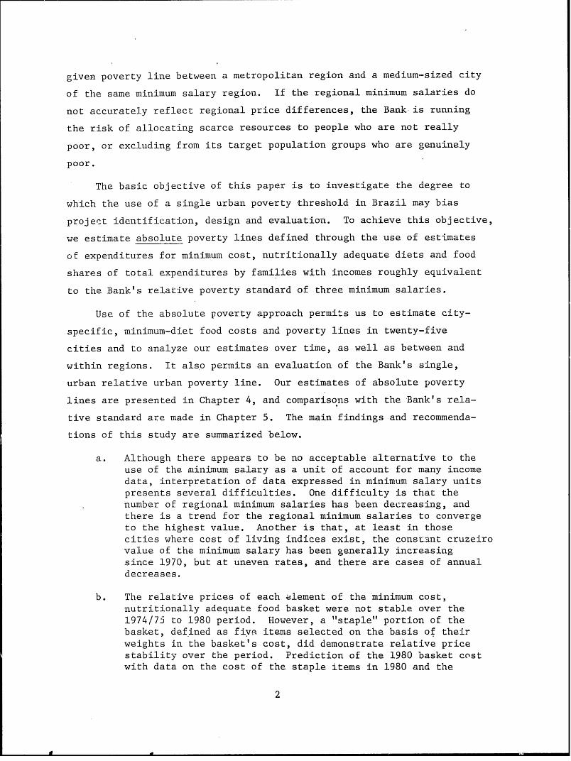
given poverty line between a metropolitan region and a medium-sized city
of the same minimum salary region. If the regional minimum salaries do
not accurately reflect regional price differences, the Bank is running
the risk of allocating scarce resources to people who are not really
poor, or excluding from its target population groups who are genuinely
poor.
The basic objective of this paper is to investigate the degree to
which the use of a single urban poverty threshold in Brazil may bias
project identification, design and evaluation. To achieve this objective,
we estinmate absolute poverty lines defined through the use of estimates
of expenditures for minimum cost, nutritionally adequate diets and food
shares of total expenditures by families with incomes roughly equivalent
to the Bank's relative poverty standard of three minimum salaries.
Use of the absolute poverty approach permits us to estimate city-
specific, minimum-diet food costs and poverty lines in twenty-five
cities and to analyze our estimates over time, as well as between and
within regions. It also permits an evaluation of the Bank's single,
urban relative urban poverty line. Our estimates of absolute poverty
lines are presented in Chapter 4, and comparisons with the Bank's rela-
tive standard are made in Chapter 5. The main findings and recommenda-
tions of this study are summarized below.
a. Although there appears to be no acceptable alternative to theuse of the minimum salary as a unit of account for many incomedata, interpretation of data expressed in minimum salary unitspresents several difficulties. One difficulty is that thenumber of regional minimum salaries has been decreasing, andthere is a trend for the regional minimum salaries to convergeto the highest value. Another is that, at least in thosecities where cost of living indices exist, the constant cruzeirovalue of the minimum salary has been generally increasingsince 1970, but at uneven rates, and there are cases of annualdecreases.
b. The relative prices of each element of the minimum cost,ntutritionally adequate food basket were not stable over the1974/75 to 1980 period. However, a "staple" portion of thebasket, defined as five items selected on the basis of theirweights in the basket's cost, did demonstrate relative pricestability over the period. Prediction of the 1980 basket costwith data on the cost of the staple items in 1980 and the
2
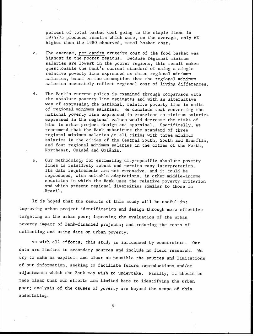
percent of total baskeL cost going to the staple items in1974/75 produced results which were, on the average, only 6%higher than the 1980 observed, total basket cost.
c. The average, per capita cruzeiro cost of the food basket wasAighest in the poorer regions. Because regional minimumsalaries are lowest in the poorer regions, this result makesquestionable the Bank's current standard of using a singlerelative poverty line expressed as three regional minimumsalaries, based on the assumption that the regional minimumsalaries accurately reflect regional cost of living differences.
d. The Bank's current policy is examined through comparison withthe absolute poverty line estimates and with an alternativeway of expressing the national, relative poverty line in unitsof regional minimum salaries. We conclude that converting thenational poverty line expressed in cruzeiros to minimum salariesexpressed in the regional values would decrease the risks ofbias in urban project design and appraisal. Specifically, werecommend that the Bank substitute the standard of threeregional minimum salariestin all cities with three minimumsalaries in the cities of the Central South, South and Brasilia,and four regional minimum salaries in the cities of the North,Northeast, Cuiaba and Goiania.
e. Our methodology for estimating city-specific absolute povertylines is relatively robust and permits easy interpretation.Its data requirements are not excessive, and it could bereproduced, with suitable adaptations, in other middle-incomecountries in which the Bank uses the relative poverty criterionand which present regional diversities similar to those inBrazil.
It is hoped that the results of this study will be useful in:
-mproving urban project identification and design through more effective
targeting on the urban poor; improving the evaluation of the urban
poverty impact of Bank-financed projects; and reducing the costs of
collecting and using data on urban poverty.
As with all efforts, this study is influenced by constraints. Our
data are limited to secondary sources and include no field research. We
try to make as explicit and clear as possible the sources and limitations
of our information, seeking to faciliate future reproductions and/or
adjustments which the Bank may wish to undertake. Finally, it should be
made clear that our efforts are limited here to identifying the urban
poor; analysis of the causes of poverty are beyond the scope of this
undertaking.
3
2, GENERZAL METHODOLOGICAL CONSlDERATIONS
2.1. Overview
The methodology used seeks to estimate absolute poverty lines in
Brazilian cities. To be useful in comparison with the World Bank's
relative poverty line estimates, our absolute poverty line estimates
should be developed so as to permit comparisons over time and between
cities. These objectives obviously impose more rigorous data require-
ments than a single, national poverty line. Our major sources of data
are discussed in Sections 2.2 and 2.3 of this Chapter.
A substantial debate has developed in the literature regarding the
use of relative versus absolute poverty measures.-/ Our purpose here is
not to directly contribute to this debate; we simply seek to evaluate
the use of a single, national, relative poverty line through the use of
absolute poverty measures which may be estimated through time and over
space.
Given the objectives and constraints of the present study, Vinod
Thomas has presented a particularly useful approach_-/ which has the
additional advantage of already being extended to Brazil.-/
Although Thomas' methodology does not have exactly the same focus
as our study (his is not limited to urban poverty), he is, as we are,
centrally concerned with the spatial variable in measuring poverty, and
the data requirements of his methodology are compatible with our constraints.
-/See, for example: Modlie Orshansky, "How Poverty is Measured,"National Labor Review (February 1969); Amartya Sen, "Issues in theMeasurement of Poverty." Scandinavian Journal of Economics, Vol. 82(1979); Theo Goedhart et al., "The Poverty Line: Concept and Measure-ment," The Journal of Human Resources, Vol. 12.
2/- Vinod Thomas, "Spatial Differences in Poverty: The Case of
Peru", Journal of Development Economics, Vol. 7 (1980), pp. 85-98.Henceforth cited as Thomas-Peru.
-/Vinod Thomas, "Differences in Income, Nutrition and Povertywithin Brazil," Washington, D.C.: The World Bank, mimeo. Draft copy(September 1981). Henceforth cities as Thomas-Brazil.
4
The essential steps of Thomas' methodology may be summarized as follows:
(M) Definition of a single basket relevant to the lowincome population (lower twentieth percentile of theincome range) of a base region (Peru's Rural SierraRegion), adjusted to meet given nutritional requirements(Peru's National Planning Institute).
(ii) Considering total expenditures as limited to two basiccategories, food and non-food, the prices of the foodcategories in the food basket were converted into re-gional relative prices, weighted according to the impor-tance of each category in the national average budget.Similarly, a regional non-food price index was cor tructed.In this way, each region's food and non-food price indicescoUld be compared to the base region, Rural Sierra.
(iii) Considering the food basket defined in (i) as the minimumrequirement at the poverty line,, measurement of theminimum food basket costs and non-food costs in RuralSierra permitted the estimation of poverty line expendi-tures in the other regions through the use of inter-regional food and non-food price indices, as developed in(ii).
Our methodology essentially follows the same steps as that of
Thomas, with the adjustments necessary to take into account differences
in study scope and the data available in Peru and Brazil. It may be
broadly described as follows:
(i) Definition of a single family food basket relevant to thelow income population (public, low-cost housing projects)of a base urban area (Rio de Janeiro), adjusted to meetgiven nutritional standards (Getulio Vargas Foundation'sinterpretation of FAO/WHO standards for the surveyedpopulation) - described in Chapter 3 and Annex II of thispaper.
(ii) Of the 25 Braziliani cities included in our survey, IBGE's -/National Household Expenditure Survey - ENDEF conductedAugust 1974-August 1975, provides directly the food share(s) of total, low-income family expenditures in 10 of thecities, and the s of the remaining cities could be inferredon a regional basis. In addition, we have direct informa-tion from IBGE's National Price Survey (Inquerito
4/- IBGE, Instituto Brasileiro de Geogtafia e Estatistica, Brazil's
Census and Statistical Office.
5
Nacional de Precos), on the prices, in each of the 25
cities for the period 1974-80, of each of the conmoditiesof the basic food basket. Thus, it was not necessary to
estimate regional price indices for food and non-foodexpenditures, as Thomas did.
(iii) Considering the family food basket defined in (i) asthe minimum requirement at the poverty line, family
poverty line expenditures for each city are estimated for
1974/75 and 1980 by dividing the expenditures necessaryto purchase the weighted food elements of the basket by
the food share (s) of total expenditures, as presented in
Chapter 4.
We readily recognize that our approach to measuring absolute poverty
lines contains arbitrarities and ambiguities. It is important, therefore,
to examine the characteristics, both weak and strong points, of our
methodology.
Disaggregation of total expenditures into only two groups, food and
non-food may be considered "heroic". It is desirable to disaggregate
non-food consumption items in other components which could be considered
to be vital to individual and family welfare, such as shelter, water and
sanitary facilities, clothing, health services and access to employment
and other. urban opportunities. Thomas recognizes-the desirability of
incorporating such components explicitly in the analysis but states that
the Peruvian data do not permit this. 5/ In the case of Brazil, it may
be possible to develop detailed family consumption structures for the
metropolitan regions. These structures are potentially available in the
ENDEF. Access to them requires, however, official permission and special
computer tabulations, which would require time and costs beyond the
scope of this study.
Even if many would argue that adequate food consumption is not
sufficient,, few would disagree that nutrition levels are necessary to
the analysis of a poverty line. There appear to be few, if any, signi-
ficant exceptions to Engels' observation that the proportion of total
expenditures allocated to food tends to decline with increasing levels
of expenditures.
-/Thomas-Peru, p. 87.
6
Increasing food proportions, s, with lower incomes, raises another
question regarding our methodology. We are placed in the uncomfortable
position, in using a city-specific s, of stating that tne poorer the
family (higher s) the less the family needs to meet the poverty line.
While there may be a wide consensus that a high proportion of total
family expenditures necessary to attain a nutritionally adequate diet
(say, over 70%), certainly is an indicator that the family lives in
absolute poverty, dividing the food expenditure amount by s to obtain
the poverty line, as we do, implies that, for a given food expenditure,
the greater the s, the lower the poverty line.
Perhaps for most of the poorest part of Brazil, especially the
Northeast, physical shelter unit quality and clothing may not be essential
to physical survival, because of the generally temperate climate.
Nevertheless, a high s for the poorest areas may mean that the poorest
families need to allocate so much of their income to nutritional survival
that the opportunity cost in terms of other important goods and services,
particularly health and sanitation services and transportation to job
opportunities, may be very high. In other words, a poverty line based
on a city-specific s may indicate an income necessary for survival, but
it could seriousiy underestimate the income level necessary to move out
of poverty.
In raising these questions about the use of s, we recognize that it
may be a potentially weak point in our methodology. Chapter 4 presents
further analysis of this consideration. This may not be a serious
problem from the Bank's perspective, however, as long as the poverty
lines presented are understood to explicitly consider only minimum
nutrition standards. Thus, one way to interpret the Bank's role is that
of helping diminish the high opportunity costs of nutrition in terms of
shelter, water, sanitation, transport and other services through urban
projects.
Another question regarding our methodology is the use of only one
nutritionally adequate food basket for all cities and for both periods.
Some may argue that nutritional requirements are subject to "adaptive
7
Yneclianisins" -over time. Although recognizing the probleins of an uncriti-
cal use of the "nutritional approach", Sen argues that:
"It is possible to overlook a simple point, to wit, mal-nutrition can provide a basis for a standard of povertywithout poverty being identified as the extent of mal-nourishment. The level of income at which an average per-son will be able to meet his nutritional requirements hasa claim to being considered as an appropriate poverty lineeven when it is explicitely recognized that nutritionalrequirements vary interpersonally around the average."
A more serious question regarding the use of a single nutritionally
adequate food basket is that it does not incorporate intercity consump-
tion preferences or commodity substitution as the result of relative
price changes. 7/ In the case of preferences, these could be regionally
adjusted for 1974/75 through detailed examination of unpublished ENDEF
data, but this would require special tabulations beyond this study's
scope. As for substitutions because of relative price changes, this is
a common index problem, and there is no easy solution. It is similar to
the Consumer Price Index problem: the Paasche Index may be considered
superior to that of Laspeyres, but the latter is usually preferred
because of cost and operational constraints. Our use of a single basket
for all the cities over the study period assumes that neither consump-
tion preferences vary significantly over space, nor that relative prices
have changed significantly over time. These assumptions will be examined
as part of the analysis presented in Chapter 4.
Although the questions raised here, and perhaps others, are signi-
ficant and should be carefully considered in interpreting our results,
the proposed methodology has a number of characteristics which recommend
it. First, it is relatively simple, and data demands are not excessive.
Once the food basket and s are established, poverty calculations are
6/ Amartya Sen, Levels of Poverty: Policy and Change, (Washington,D.C.: The World Bank, Staff Working Paper No. 401, July 1980), p.4.Emphasis in original.
7/I
-/The food shares calculated from the 1974/75 ENDEF and the commodityweights calculated from the 1973 Getulio Vargas Foundation survey (seeChapter 3) were assumed to be constant over the 1974-80 period. Morerecent estimates are not available.
8
simple and several sensitivity tests may be performed with relatively
easy interpretations.' This facilitates reproduction (new studies in
other middle-income countries and up-dates in Brazil) aind comparison
(with other countries or later periods in Brazil).
Second, particularly in Brazil, where systematic, local commodity
prices to the consumer are available..over time, the methodology permits
a relatively high degree of rigor in city-specific costing of the mini-
mum food basket, as well as the evaluation of some of the potentially
negative aspects of the methodology, as raised earlier, over time.
Finally, given that the methodology is relatively simple and robust,
it permits (see Chapter 4) quickly obtained instrumental, or "short-
cut", estimates of the poverty line in a city not covered in the survey
(or a surveyed city at a later date) through readily available data at a
low cost.
2.2 The Unit of Analysis
Although a large proportion of the studies of income distribution
done in Brazil to date has concentrated on the individual (economically
active population), there seems to be a broad consensus in the litera-
ture that for the study of poverty the family or household unit is the
most adequate unit of analysis. Since most people live in family groups,
what defines poverty is the income available to be shared among family
members. As Kuznets has put it, "in a meaningful distribution of income
by size, the recipient unit has to be the family or household and cannot
be a person." 81
The use of the family or household as the unit of analysis raises
the question of whether total or per capita measures of family or house-
hold income should be used. Musgrove - argues forcef'ully in favor of the
8/Simon Kuznets, "Demographic Aspects of Size Distribution of
Income. An Exploratory Essay", Economic Development and Cultural Change,Vol. 25 (October 1975) p.l.
9'Philip Musgrove, "Household Size and Composition, Employment andPoverty in Urban Latin America", Economic Development and Cultural Change,'Vol. 28, No. 2 (January 1980), p. 250.
9
per capita measure simply because "the variation in family size among
households is much too great to be ignored when describing income dis-
tribution."
For the present study, we shall use the family as the basic unit of
analysis. For each city in our survey, we estimate the poverty line for
a family of average (mean) size for a broader view of poverty within
that city. In addition, the per capita family poverty line income is
estimated, in order to permit the analysis of the distribution of family
sizes on the poverty line. We draw our definition of the fJamily from
ENDEF, considering the base for family definition as the "budget unit
expenditures". Thus, the family unit is considered on the basis of a
common dwelling unit and a unified income and expenditure budget, -
2.3 The Instruments of Measurement
In estimating the absolute poverty line for each of the 25 Brazilian
cities we relied on four major sources of data: regional minimum salaries;
ENDEF; the National Price Survey; and the Getulio Vargas Foundation.
Below, an, overview of these sources is presented, including their relatively
strong and weak points.
2.3.1 Regional Minimum Salaries
The minimum salary in Brazil is defined periodically by law.
Historically, the minimum salary has changed each year on May 1st, but
since 1979, there are two changes per year, May and November. These
changes are supposed to reflect changes in the cost of living, but the
actutal methodology for calculation is not made public.
For this study, the minimum salary is most important as a unit of
account. Not only are most low-income urban workers directly affected
by its value, a great deal of published data regarding income distribution
is presented in minimum salary intervals. Also, given the high rates of
1-/For a more detailed description of the ENDEF's units of analysis,see Paulo T.A. de Andre, "The Brazil 1974/75 National Household ExpenditureSurvey", Conducting Surveys in Developing Countries: Practical Problemsand Experiences in Brazil, Malaysia and the Philippines (Washington,D.C.: The World Bank Living Standards Measurement Study Working PaperNo. 5), pp. 24-43.
10
inflation in Brazil, transforming income or expenditures in minimum
salary units is important in interpreting intertemporal and regional
trends.
The poverty lines in 25 cities at two points in time are presented
in Chapter 4, and much of their interpretation depends cn our under-
standing of the minimum salary. Our poverty lines are based on the
incomes at the beginning of the periods covered by our survey of the
costs of the minimum food basket. This is based on the assumption that,
for most of the target group, incomes were relatively constant over the
minimum salary period. With high inflation over the period, however,
the buying power of incomes tended to decrease.
Our temporal base is for the period of the ENDEF study, August 1974
to August 1975. Therefore, the most relevant minimum salary period is
from May 1, 1974 to April 30, 1975. We also calculate the poverty lines
in 1980. In that year, however, the minimum salary changed twice, on
May 1st and November 1st. We have used the May 1st 1980 mimimum salary
as our unit of account.
Although it is very difficult, if not impossible for all but the
few who actually make the decisions regarding mirimum salary changes, to
examine the change criteria, certain tendancies over time may be noted.
First, there has been a recent reduction in the concentration of wage
earners at the one minimum salary level. In 1970, 60.6% of the econo-
mically active population earned one minimum salary or less and 82.3%
two or less; in 1976 these figures were, respectively 37.4% and 66.8%.ll/
Table 1 demonstrates another tendency, of a dramatic loss of rela-
tive buying power of the minimum salary during the 1960's, and relative
stability (although at a lower level than the early 1960's) since 1975.
However, it is important to note that 1974 presented a significant
decrease, especially since the 1974 minimum salary is the base point for
our study.
-/IBGE, Indicadores Socialis-1979, p. 185.
*11
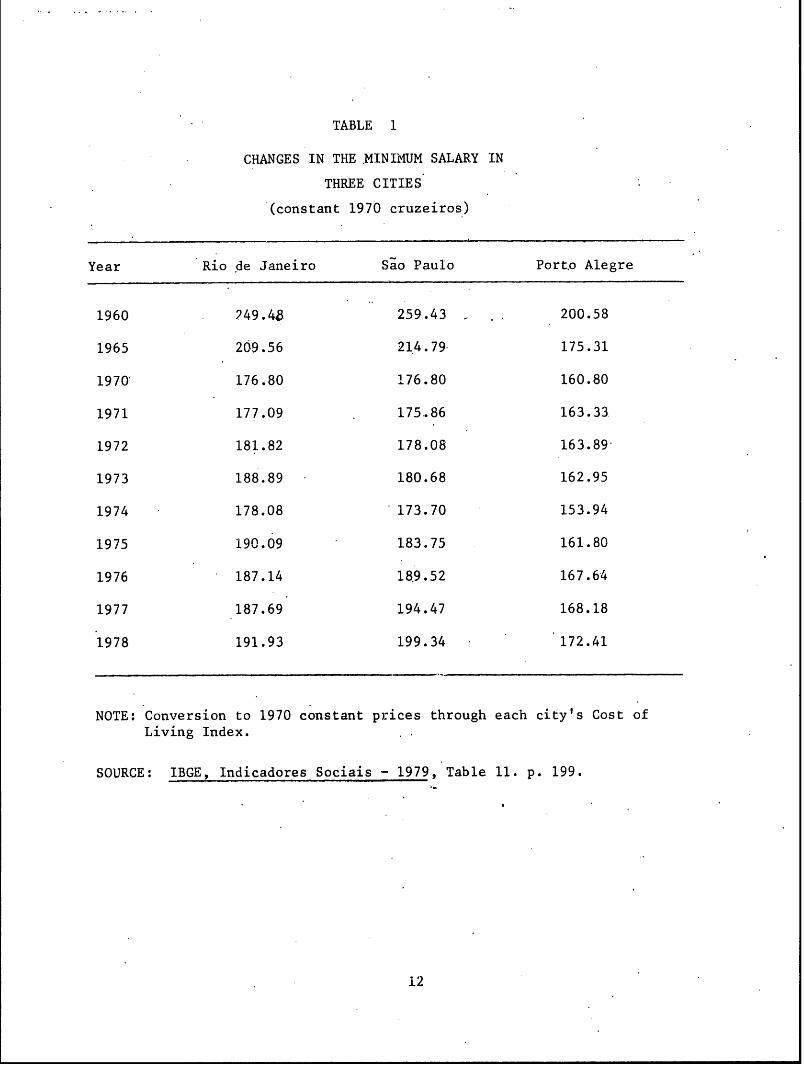
TABLE 1
CHANGES IN THE MINIMUM SALARY IN
THREE CITIES
(constant 1970 cruzeiros)
Year Rio de Janeiro Sao Paulo Porto Alegre
1960 249.48 259.43 200.58
1965 209.56 214.79 175.31
1970 176.80 176.80 160.80
1971 177.09 175.86 163.33
1972 181.82 178.08 163.89
1973 188.89 180.68 162.95
1974 178.08 173.70 153.94
1975 190.09 183.75 161.80
1976 187.14 189.52 167.64
1977 187.69 194.47 168.18
1978 191.93 199.34 172.41
NOTE: Conversion to 1970 constant prices through each city's Cost ofLiving Index.
SOURCE: IBGE, Indicadores Sociais - 1979, Table 11. p. 199.
12
Table 2 presents the 1974 and 1980 minimum salaries used in this
study, as well as indices of change in the regional minimum salaries
over time,. for each of the cities in our survey. Two important trends
are clear. First, the degree of "fine-tuning" for the minimum salary
has greatly decreased: from 14 different values in 1960, 1974 presented
5 and 1980 only 3. This is an indication that there may be one national
minimum salary in the near future. Another trend has been decreased
dispersion from the highest minimum salary. In 1960, the lowest minimum
salary (Teresina) was 42% of the highest (Rio de Janeiro); in 1970 the
difference decreased to 67% and in 1980 to 77%. If the cost of living
in those cities with minimum salaries lower than the highest has been
increasing at about the same rates as Rio de Janeiro and Sao Paulo, then
a comparison of the data of Tables 1 and 2 indicates that the lower
minimum salaries have been increasing faster than the cost of living in
those cities.
2.3.2 National Household Expenditure Survey - ENDEF
Another important source of data is the ENDEF, which presents
detailed family expeuiditure data. After a careful review of income
sources in Brazil, Pfeffermann and Webb conclude that ENDEF "provides
the most reliable basis for statements about the structure of income.
Expenditure surveys usually achieve better coverage of total income than
employment surveys and this was the case with ENDEF. 1 2/
ENDEF is particularly important for this study in that it provides
us with key variables, especially the food expenditure share (s) of
total family expenditures and average family size. In some cases,
however, ENDEF aggregates our sample cities in larger urban units,
because ENDEF provides urban information by 15 urban regions. In those
cases, we consider family size and the food share as equal in each of
the cities of the ENDEF urban region. This occurs in the following
1-2/Guy P. Pfeffermann and Richard Webb, The Distribution of Incomein Brazil; (Washington, D.C.: The World Bank Staff Working Paper No.356, September 1979), pp. 13-14. See especially pp. 7-37 for a reviewof income data.
13
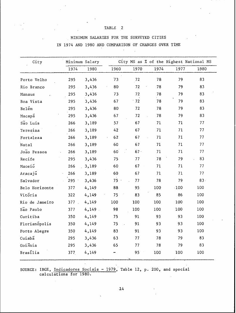
TABLE 2
MINIMUM SALARIES FOR THE SURVEYED CITIES
IN 1974 AND 1980 AND COMPARISON OF CHANGES OVER TIME
City Minimum Salary City MS as % of the Highest National MS
1974 1980 1960 1970 1974 1977 1980
Porto Velho 295 3,436 73 72 78 79 83
Rio Branc-o 295 3,436 80 72 78 79 83
Manaus 295 3,436 73 72 78 79 83
Boa Vista 295 3,436 67 72 78 79 83
Belem 295 3,436 80 72 78 79 83
Macapa 295 3,436 67 72 78 79 83
Sao Luis 266 3,189 57 67 71 71 77
Teresina 266 3,189 42 67 71 71 77
Fortaleza 266 3,189 62 67 71 71 77
Natal 266 3,189 60 67 71 71 77
Joao Pessoa 266 3,189 60 . 67 71 71 77
Recife 295 3,436 75 77 78 79 . 83
Macei6 266 3,189 60 67 71 71 77
Aracaju 266 3,189 60 67 71 71 77
Salvador 295 3,436 75 . 77 78 79 83.
Belo Horizonte 377 4,149 88 95 100 .100 100
Vitoria 322 4,149 75 83 85 86 100
Rio de Janeiro 377 . 4,149 100 100 100 100 100
Sao Paulo 377 4,149 . 98 100 100 100 100
Curitiba 350 4,149 75 91 93 93 100
Florianopolis 350 4,149 75 . 91 93 93 100
Porto Alegre 350 4,149 83 91 93 93 100
Cuiaba 295 3,436 63 77 78 79 83
Goi"ania 295 3,436 65 77 78 79 83
Brasilia 377 4,149 - 95 100 100 100
SOURCE: IBGE, Indicadores Sociais - 1979, Table 12, p. 200, and specialcalculations for 1980.
*14
cases:
(i) Porto Velho, Rio Branco, Manaus, Boa Vista and Macapa;
(ii) Sao Luis, Teresina, Natal, Joao Pessoa, Maceio and Aracaju;
(iii) Cuiaba and Goiania
In additiorn to the aggregated data for the 13 cities above, ENDEF
provides separate family size and food share data for each of the nine,
metropolitan regions and Brasilia (including not only the Plano Piloto,
but also the "satellite cities"). Vitoria and Florianopolis are the
only surveyed cities of other ENDEF regions (regions 8 and 11 respecti-
vely). Annex III presents the ENDEF regions.
In estimating the food share (s) of total family expenditures, we
used the ENDEF annual family income interval of Cr$ 9,000 to Cr$ 15,799
for August 1974 income levels. In May 1974 minimum salary terms, this
interval corresponded to 2.0 to 3.5 MS in the Southeast (except Vitoria),
2.1 to 3.8 for the South, 2.5 to 4.5 for the Center West and Amazon and
2.8 to 4.9 for most of the Northeast, except Recife and Salvador, which
had Center-West levels. This is the onlv interval consistent with the
Bank's standard of 3 minimum salaries. Thus, each s and each absolute
poverty line are estimated from a base strata roughly comparable to the
Bank's relative poverty standard.
ENDEF also calculated non-monetar!r income. In the case of urban
areas, the most important source of non-monetary income is imputed
rents. In order to examine the impact of excluding this component from
total family income, we perform a sensitivity test (Annex IV) excluding
imputed rents from total income. This, of course, changes the s values.
2.3.3. National Price Survey - INP
Our source of data for costing the minimum diet food basket in
the 25 cities is the National PLrice Survey (INP). 13- In this survey,
Ai/IBGE, Inquerito Nacional de Precos: Generos AlimentL,cios, withirregular publication periods.
15
over 50 food item prices are collected monthly in retail establish-
ments of the urban areas of the capital Municipality of each State and
Territory.
For 1974/75, INP data for the third and fourth quarters of 1974 and
first and second quarters of 1975 were used. For this period, therefore,
food price data are for July 1974 to June 1975, ENDEF information for
August 1974 to August 1975, and the minimum salary applies to May 1974
to April 1975. Some small distortions may be introduced by not having
the time periods for each data source precisely consistent, but this is
the best approximation possible with the available data.
For the 1980 period, the food price data correspond to the same
period as the validity of the minimum salary, May 1980 through October
1980.
In both periods, the quality of the food price data may be considered
good. In each period, a food price matrix was developed with 25 cities
and 22 commodities (see Chapter 3). In 1974/75, 13 of the 550 matrix
cells presented the problems of product' prices not being available in
some cities. Seven of the "problem cells" were caused by the prices of
the specific type of rice of our survey (arroz japones) not being avail-
able, and they were substituted by another type of rice (arroz agulha).
Other cases involved substitution of another type of bean or taking the
relevant price from the closest city with best information. In 1980,
ce ls15/there were only six "problem cells" - and in general we conclude that
the city-specific food, price data are of good quality.
2.3.4. Getulio Vargas Foundation
Our final major source of data is the Getulio Vargas Founda-
tion's study of minimum cost diets for low-income families. Considering
- /The number of food items has varied. For example, in 1974, 56
items were collected; in 1979, there were 59.
5-/Type of bean substitution for 2 months in Rio; 2nd class meat
and chicken prices for Goiania were inferred from Campo Grande; drymeat, egg and milk prices for Boa Vista were inferred from the meanprices observed in Porto Velho, Rio Branco, Manaus and Cuiaba.
16
that the commodity weights of the food basket are one of the most
critical elements of our methodology, these are discussed in the next
chapter, with details presented in Annex II.
17
3. DEFINITION OF TllE POVERTY LINE FOOD BASKET
Definition of the poverty line food basket for this study is based
on the Getulio Vargas Foundation (FGV) nutrition study -/ conducted in
October - December 1973. A sample of 235 families living in public
housing (COHAB) apartments was examined in detail as to its physical,
socioeconomic and nutritional characteristics. 2/
The study's definitions of family unit, income and expenditures are
consistent with the later ENDEF (see FGV-Pesquisa, p. 14 and p. 86).
The mean family income of the sample was 3.4 minimum salaries, with an
average family size of 4.9 and a family per capita income of 0.69 MS.
The frequency distribution of the families by income intervals indicates,
however, that about 65% of the families had incomes of less than 3.5 MS,
and the income interval of the median value had a mean of 3.1 MS. Only
4 families had incomes greater than 8 MS, with 18 MS the upper-bound of
the last interval (FGV-Pesquisa, Table 5.1, p. 87).
This sample appears to be compatible with the type of population
the Bank generally is involved with in urban projects and is essentially
consistent with the relative poverty criterion currently in use on a
national basis. This enables us to use the general findings in developing
a relevant food basket which can be analyzed across cities over time.
Based on FAO/WHO nutritional standards interp.reted for the character-
istics of the sampled population, the nutritional quality of observed
diets is presented in Table 3.
1/- This study has two major sets of documents. Pesquisa Sobre Consumo
Alimentar, (June 1975-3 vols.) gives the study methodology and generalfindings. This study will be cited as FGV-Pesquisa, referring only toits Vol. I. Dietas de Custo Minimo: Aplicacao da Programacao Linear aAlimentacao Humana (January 1978 - Vol. 1.) is based on the former studyand analyzes in detail the nutritional quality of the observed diets, aswell as potential improvements. This study will be cited as FGV-Dietas.
2/- This sample is from the universe of 28,621 COHAB apartment units
existing.in Guanabara (now the Municipality of Rio de Janeiro) at thattime.
18
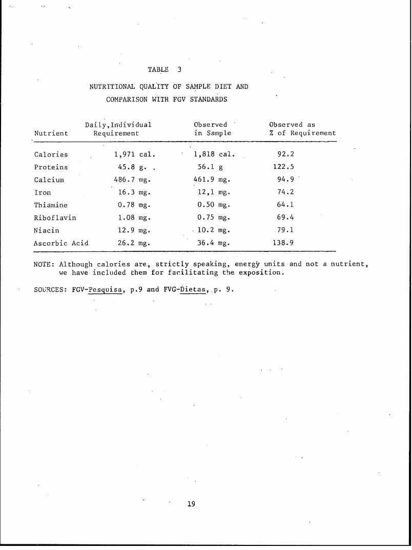
TABLE 3
NUTRITIONAL QUALITY OF SAMPLE DIET AND
COMPARISON WITH FGV STANDARDS
Daily,Individual Observed Observed asNutrient Requirement in Sample % of Requirement
Calories 1,971 cal. 1,818 cal. 92.2
Proteins 45.8 g. 56.1 g 122.5
Calcium 486.7 mg. 461.9 mg. 94.9
Iron 16.3 mg. 12,1 mg. 74.2
Thiamine 0.78 mg. 0.50 mg. 64.1
Riboflavin 1.08 mg. 0.75 mg. 69.4
Niacin 12.9 mg. 10.2 mg. 79.1
Ascorbic Acid 26.2 mg. 36.4 mg. 138.9
NOTE: Although calories are, strictly speaking, energy units and not a nutrient,we have included them for facilitating the exposition.
SOURCES: FGV-Pesquisa, p.9 and FVG-Dietas, p. 9.
19
It should be noted that the FGV interpretation of FAO/WH0O nutri-
tional requirements produced results somewhat lower than other published
figures. For example, the World Bank's Brazil: Human Resources Special
Report uses the FAO/WHO "low" requirement for per capita daily calorie3/
consumption of 2,261 as a standard of comparison. - &he major reason
for this discrepancy seems to be that the FGV reduced the FAO/WHO
standard for cal!Dries by 8.85% for a climate adjustment, and this directly
affected the thiamine, riboflavin and niacin requirements, which were41.
set as proportional to calories, for each age, sex and weight group. -
The average per capita daily calorie requirements of the ENDEF for
urban Brazil were set at 2,007 ranging from 1,807 in the Northeast to
2,086 in the urban South and Southeast regions. The FAO/WHO low require-
ment is 2,261 for average urban, with 2,150 for urban Northeast and
2,299 for urban South and Southeast. - In comparing the observed
calorie consumption of the FGV sample with the FAO/WHO standard, the
sampled population had an individual calorie deficit of 443 per day.
This deficit places the sampled population, according to the Bank's
Human Resources report for Brazil, in the lowest calorie consumption
category (deficits over 400 calories), which is estimated to include
21.9% of Brazil's total urban population, ranging from 48.7% in the
urban Northeast and 12.3% in the urban South and Southeast. The remainder
of the urban population is estimated to have an adequate diet (23.5%
urban Brazil, 29.6% South and Southeast and 8,5% Northeast) or individual
deficits of less than 400 per day. 6/
3/The World Bank, Brazil: Human Resources Special Report, (Washington,
D.C.: The World Bank, 1979) Annex III, pg. 49. Henceforth cited asWorld Bank, Human Resources.
-/FGV-Dietas, p. 8 and pp. 320-321.
5/World Bank, Human Resources, Annex III, Table 14, p. 46.
-/World Bank, Human Resources, Annex III, Table 15, p. 50.
20
The FGV nutritional standards and sample population are very important
to the present study. On them, we built our empirical base for estimating
the poverty lines. In evaluating the FGV data, we observe that, from a
nutritional perspective, the sampled population meets most definitions
of urban poverty. In addition to presenting absolute nutritional deficits,
even with low FGV requirements, some 78% of Brazilts urban population
are estimated to have better diets than the sampled population, and 88%
of the region's urban population are in. a superior position; translating
the Bank's income definition of relative poverty into nutritional terms
would surely classify the sampled population as poor. In using the FGV
diet standards we tend to introduce a conservative bias in our estimates
of the poverty line; if higher nutrition requirements were used, the
food basket would be more expensive and the poverty line higher.
The FGV sample identified 80 food products consumed by the sampled
families. These products formed the universe for the FGV linear programming
model. Basic inputs were the nutritional qualities and market prices of
each product, as well as the family nutritional requirements. The first
minimum cost solution, with only nutritional requirement constraints,
produced a diet of only 9 products at a monthly cost of Cr$ 374.79 at
1975 average prices. It is unlikely, however, that any family could
sustain such a constrained diet for very long. Its main elements are
33.9 kilos/month of wheat flour and 14.6 of manioc (cassava) flourr and
it provides no coffee or condiments. -
Another diet (titled diet "H" by the FGV) results from the introduction
of a number of "palpability" constraints, which forced the int.roduction
of widely consumed elements, such as coffee, salt and pepper, and limited
the amounts of such foods as wheat and manioc flour. This produced a
more reasonable diet, in the sense of better approximating the actual
habits of urban consumers at, however, a higher least cost, Cr$ 517.22.
This is the diet we selected to form the base of the nutritionally
adequate, least cost diet, as presented in Table 4.
7 /Other elements of this diet are black beans (7.8 kg/month), brownbeans (3.1), liver (3.1), dry meat (5.0), fresh milk (13.1), soybean oil(5.8), and kale (0.8).
21
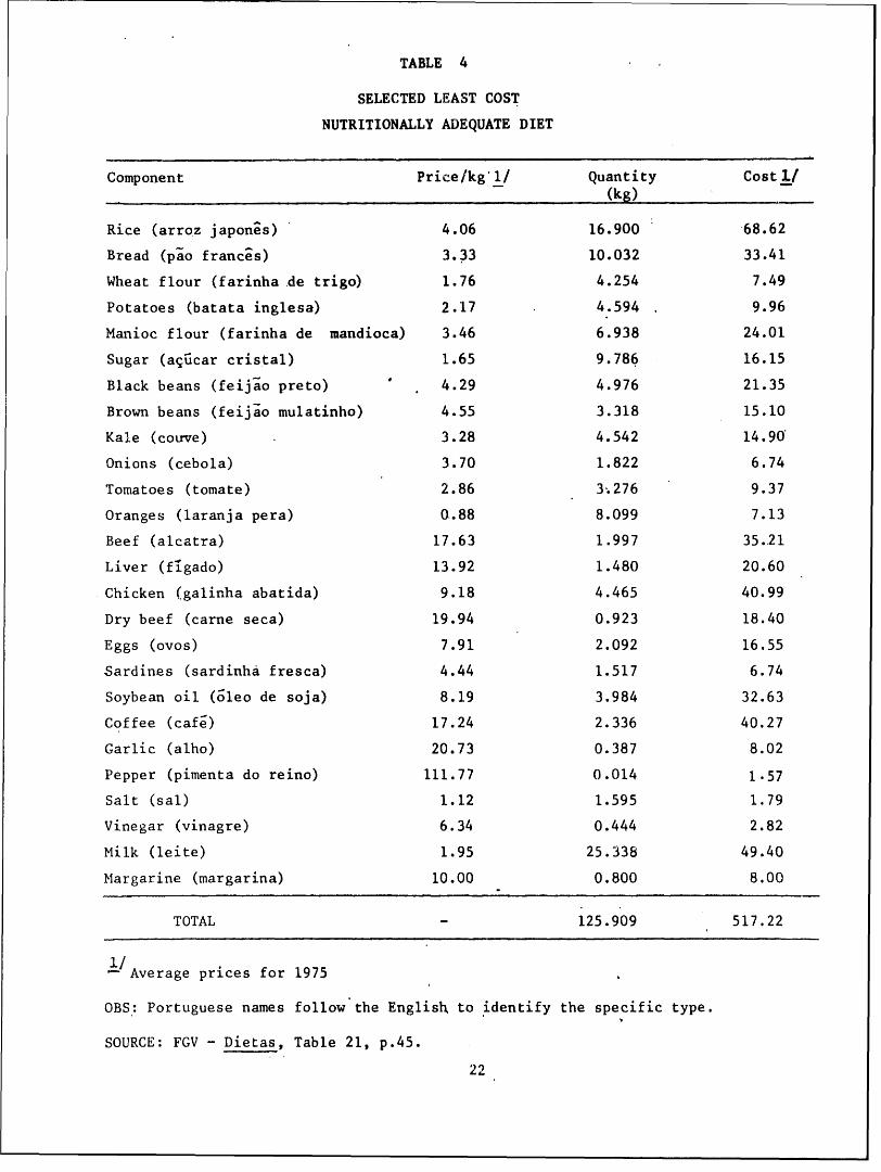
TABLE 4
SELECTED LEAST COST
NUTRITIONALLY ADEQUATE DIET
Component Price/kg 1/ Quantity Cost I,(kg)
Rice (arroz japones) 4.06 16.900 68.62
Bread (pao frances) 3.33 10.032 33.41
Wheat flour (farinha.de trigo) 1.76 4.254 7.49
Potatoes (batata inglesa) 2.17 4.594 9.96
Manioc flour (farinha de mandioca) 3.46 6.938 24.01
Sugar (agiicar cristal) 1.65 9.786 16.15
Black beans (feijao preto) 4.29 4.976 21.35
Brown beans (feijao mulatinho) 4.55 3.318 15.10
Kale (courve) 3.28 4.542 14.90
Onions (cebola) 3.70 1.822 6.74
Tomatoes (tomate) 2.86 3.276 9.37
Oranges (laranja pera) 0.88 8.099 7.13
Beef (alcatra) 17.63 1.997 35-21
Liver (figado) 13.92 1.480 20.60
Chicken (galinha abatida) 9.18 4.465 40.99
Dry beef (carne seca) 19.94 0.923 18.40
Eggs (ovos) 7.91 2.092 16.55
Sardines (sardinha fresca) 4.44 1.517 6.74
Soybean oil (oleo de soja) 8.19 3.984 32.63
Coffee (cafe) 17.24 2.336 40.27
Garlic (alho) 20.73 0.387 8.02
Pepper (pimenta do reino) 111.77 0.014 1.57
Salt (sal) 1.12 1.595 1.79
Vinegar (vinagre) 6.34 0.444 2.82
Milk (leite) 1.95 25.338 49.40
Margarine (margarina) 10.00 0.800 8.00
TOTAL 125.909 517.22
-LAverage prices for 1975
OBS: Portuguese names follow the English to identify the specific type.
SOURCE: FGV - Dietas, Table 21, p.45.
22
The next step was to compare the components of Table 4 with the
city-specific food prices of the INP. Of the 26 food items, the INP
only publishes 22. The missing items (kale, liver, sardines and pepper)
were substituted through examination of the tables -/ of the nutritional
quality of each product and manual iteration. The substitutions did not
substantially modify the nutritional quality of the diet and, in fact,
slightly reduced its cost, to Cr$ 515.50. A more detailed description
of the substitution methodology is presented in Annex II.
The food component quantities as used in calculating the poverty
lines are presented in Table 5. We consider this the minimum diet for
the FGV typical family (4.72 adult equivalents). - Its 1975 average
cost is Cr$ 515.50. Actual food expenditures of the surveyed families
were Cr$ 604.70 in 1975 prices, about 20% higher. As a sensitivity test
in Annex IV, we multiply the minimum diet by 1.2 for comparison with
whiat may be called a "behavioral diet."
-/FGV-Dietas, pp. 12-15.
9/-To simplify calculations, we opted for the "head count" metho-
dology rather than adult equivalents. Thus, in calculating povertylines, we used the quantities of Table 5 as applying to a family of 5.An evaluation of the impact of this adjustment is presented in Annex II.
23
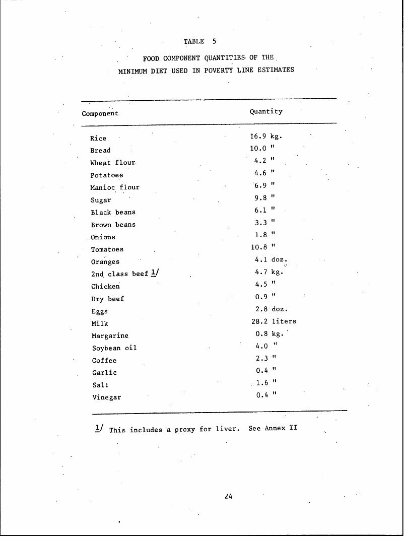
TABLE 5
FOOD. COMPONENT QUANTITIES OF THE
MINIMUM DIET USED IN POVERTY LINE ESTIMATES
Component Quantity
Rice 16.9 kg.
Bread 10.0 "
Wheat flour. 4.2 "
Potatoes 4.6 "
Manioc flour 6.9 "
Sugar 9.8 "
Black beans 6.1 "
Brown beans 3.3 "
Onions 1.8 "
Tomatoes 10.8 "
Oranges 4.1 doz.
2nd. class beef 1/ 4.7 kg.
Chicken' 4.5
Dry beef 0.9 "
Eggs 2.8 doz.
Milk 28.2 liters
Margarine 0.8 kg.
Soybean oil 4.0 "
Coffee 2.3 "
Garlic 0.4 "
Salt 1.6 "
Vinegar 0.4"
l/ This includes a proxy for liver. See Annex II
24
4. ESTIMATES AND ANALYSIS OF THE ABSOLUTE POVERTY LINES
This chapter is limited to presentation and analysis of the absolute
poverty lines in the 25 surveyed cities. Comparison of these findings
with the World Bank's relative poverty lines is presented in the following
chapter.
Section 4.1 simply presents the absolute estimates. Sections 4.2-
4.4 analyze the estimates from intertemporal, city size and regional
perspectives.
4.1 Absolute Poverty Line Estimates Based on Minimum Diet Costs
Tables 6 and 7 present estimates of absolute poverty lines in the
25 surveyed cities. The estimates are based on the cost of the minimum
cost, nutritionally adequate diet, the food share of total family expen-
ditures, and average family size in each city.
Interpretation of the estimates presented in Tables 6 and 7 should
be guided by the following summary of the characteristics of the methodol-
ogy used.
(i) Per capita costs of the minimum diet in 1974-75 and 1980(Columns 1 and 2 of Table 6) may be considered to be the leastbiased of the poverty indicators, in that they are deriveddirectly from field observation and are not influenced bysubsequent steps of the methodology. The 1974-75 figuresshould be very close to reality if the food basket quantities(Table 5) derived from Rio de Janeiro data are valid acrossthe regions. The 1980 figures may be less accurate, giventhat the basket quantities are constant for both periods andthus do not incorporate changes in consumption behavior whichmay have occurred over the period because of changes inrelative food prices. This question is addressed in thefollowing section.
(ii) The food share (s) is considered constant for both estimateperiods. This assumes that preferences and relative food andnon-food prices have not changed significaAtly over the period.
(iii) Average family size was calculated.from ENDEF data (as was s)and corresponds to the 1974/75 peUiod, although in some casesa sample city's average family size had to be taken fromaggregated, regionalized ENDEF data (see Section 2.3 - thisaggregation also applied to s data). Some implications of
25
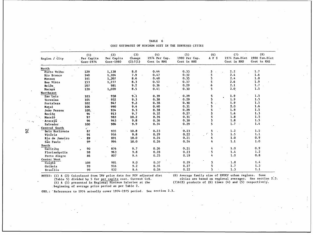
TABLE 6
COST ESTIMATES OF MINIMUM DIET IN TILE SURVEYED CITIES
(1) (2) (3) (4) (5) (6) (7) (8)
Region / City Per Capita Per Capita Change 1974 Per Cap. 1980 Per Cap. A F S 1974 Fam.Diet 1980 Fam.Diet
Cost-1974 Cost-1980 (2)/(1) Cost in RMS Cost in RMS Cost in RMS Cost in REMS
NorthPorto Velho- 129 1,138 8.8 0.44 0.33 5 2.2 1.7
Rio Branco 140 1,104 7.9 0.47 0;32 5 2.4 1.6
Manaus 141 1,207 8.6 0.48 0.35 5 2.4 1.8
Boa Vista 153 1,277 8.3 0.52 0.37 5 2.6 1.9
Belim 107 981 9.2 0.36 0.29 6 2.1 1.7
Mac'api 120 1,020 8.5 0.41 0.30 5 2.0 1.5
NortheastSao Luis 103 938 9.1 0.39 0.29 5 1.9 1.5
Teresina 101 932 9.3 0.38 0.29 5 1.9 1.5
Fortaleza 102 947 9.3 0.38- 0.30 5 1.9 1.5
Natal 106 990 9.4 0.40 0.31 5 2.0 1.6
Joao Pessoa 100, 934 9.3 0.38 0.29 5 1.9 1.5
Recife 94 913 9.7 0.32 0.27 5 1.6 1.3
Maceio 97 983 10.2 0.36 0.31 5 1.8 1.5
Aracaju . 96 943 9.8 0.36 0.30 5 1.8 1.5
Salvador 100 986 9.9 0.34 0.29 5 1.7 1.4
Central SouthBelo Hurizonte 87 935 10.8 0.23 0.23 5 1.2 1.1
Vitoria 94 916 9.8 0.29 0.22 , 5 1.5 1.1
Rio de Janeiro 89 891 10.0 0.24 0.21 4 1.0 0.9
Sao Paulo 99 - 994 10.0 0.26 0.24 4 1.1 1.0
SouthCuritiba 90 876 9.7 0.26 0.21 4 1.0 0.9
Florianopolis 98 963 9.8 0.28 0.23 5 1.4 1.2
Porto Alegre 86 807 9.4 0.25 0.19 4 1.0 0.8
Center WestCuiaba 108 981 9.0 0.37 , 0.29 5, 1.8 1.4
Goiania 99 916 9.2 0.34 0.27 5 1.7 1.3
Brasilia 99 932 9.4 0.26 0.22 5 1.3 1.1
NOTES: (1) & (2) Calculated from INP price data for FGV adjusted diet (6) Average family size of ENDEF urban regions. Some
(Table 5) divided by 5 for per capita cost. Current Cr$. cities are based on regional averages. See section 2.3.
(4) & (5) presented in Regional Minimum Salaries at the (7)&(8) products of (6) times (4) and (5) respectively.
beginning of average price period as per Table 2.
OBS.: -References to 1974 actually cover 1974-1975 period. See section 2.3.
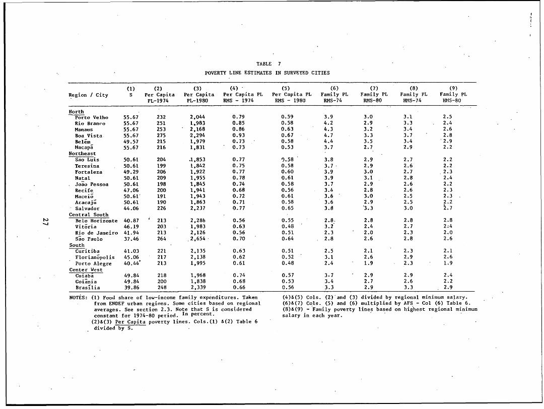
TABLE 7
POVERTY LINE ESTIMATES IN SURVEYED CITIES
(1) (2) (3) (4) (5) (6) (7) (8) (9)Region / City S Per Capita Per Capita Per Capita PL Per Capita PL Family PL Family PL Family PL Family PL
PL-1974 PL-1980 REMS - 1974 RMS - 1980 RMS-74 REMS-80 HMS-74 HMIS-80
NorthPorto Velho 55.67 232 2,044 0.79 0.59 3.9 3.0 3.1 2.5Rio Branc-o 55.67 251 1,983 0.85 0.58 4.2 2.9 3.3 2.4Manaus 55.67 253 2,168 0.86 0.63 4.3 3.2 3.4 2.6Boa Vista 55.67 275 2,294 0.93 0.67 4.7 3.3 3.7 2.8Belem 49.57 215 1,979 0.73 0.58 4.4 3.5 3.4 2.9Nacapa 55.67 216 1,831 0.73 0.53 3.7 2.7 2.9 2.2
NortheastSao Luis 50.61 204 .1,853 0.77 3.58 3.8 2.9 2.7 2.2Teresina 50.61 199 1,842 0.75 0.58 3.7 2.9 2.6 2.2Fortaleza 49.29 206 1,922 0.77 0.60 3.9 3.0 2.7 2.3Natal 50.61 209 1,955 0.78 0.61 3.9 3.1 2.8 2.4Joao Pessoa 50.61 198 1,845 0.74 0.58 3.7 2.9 2.6 2.2Recife 47.06 200 1,941 0.68 0.56 3.4 2.8 2.6 2.3Haceio 50.61 191 1,943 0.72 0.61 3.6 3.0 2.5 2.3Aracaju 50.61 190 1,863 0.71 0.58 3.6 2.9 2.5 2.2Salvador 44.06 226 2,237 0.77 0.65 3.8 3.3 3.0 2.7
Central SouthBelo Horizonte 40.87 213 2,28b 0.56 0.55 2.8. 2.8 2.8 2.8Vitoria 46.19 203 1,983 0.63 0.48 3.2 2.4 2.7 2:4Rio de Janeiro 41.94 213 2,126 0.56 0.51 2.3 2.0 2.3 2.0Sao Paulo 37.46 264 .2,654 0.70 0.64 2.8 2.6 2.8 2.6
SouthCuritiba 41.03 221 2,135 0.63 0.51 2.5 2.1 2.3 2.1Florianopolis 45.06 217 2,138 0.62 0.52 3.1 2.6 2.9 2.6Porto Alegre 40.44 213 1,995 0.61 0.48 2.4 1.9 2.3 1.9
Center WestCuiaba 49.84 218 1,968 0.74 0.57 3.7 2.9 2.9 2.4Goi^ania 49.84 200 1,838 0.68 0.53 3.4 2.7 2.6 2.2Brasilia 39.86 248 2,339 0.66 0.56 3.3 2.9 3.3 2.9
NOTES: (1) Food share of low-income family expenditures. Taken (4)&(5) Cols. (2) and (3) divided by regional minimum salary.from ENDEF urban regions. Some cities based on regional (6)&(7) Cols. (5) and (6) multiplied by AFS - Col (6) Table 6.averages. See section 2.3. Note that S is considered (8)&(9) - Family poverty lines based on highest regional minimumconstant for 1974-80 period. In percent. salary in each year.
(2)&(3) Per Capita poverty lines. Cols.(l) &(2) Table 6divided by S.
changes in average family size are discussed in Annex IV, and
the 1980 estimates are based on the same family size data asused in 1974/75.
(iv) The number of regional minimum salaries decreased from 5 in
1974, to 3 in 1980 (see Section 2.3).
4.2 Intertemporal Changes in the Poverty Line
One of the most striking results presented in Table 7 is the significant
decrease in the absolute poverty line estimates over time. With only.
one exception (Belo Horizonte), the estimates expressed in terms of
regional minimum salaries (Cols. 6 and 7) decreased substantially from
the 1974/75 period to 1980. In general, the estimates decreased less
sharply in the metropolitan regions of the South and Central South than
in other cities.
Considering that the absolute poverty line estimates are based on a
given food basket, one possible explanation of this decrease is that the
food basket cost has increased at a rate lower than that of the minimum
salaries. Although changes in regional minimum salaries have not necessarily
been directly proportional to changes in the cost of living, the FGV
General Price Index-!/ indicates that the cost of living in Rio de
Janeiro has increased by'a factor of 11.4 at current prices from August
.1974 to August 1980. Comparison of this change with Col. 3 of Table 6
lends some support to the hypothesis that food prices have been increasing
at a lower rate than general prices. This is a question which remains
open, however, given our limitation of having available only one food
basket for both periods and for all cities. -/
-/From FGV, "Indices Economicos - Suplemento Especial," Conjuntura
Economica, Vol. 33, No. 11, p. 10 - ''Coluna 2."
-'Analysis of variance of the price of each food item of our basket
by aggregated PNAD regions was done. The sampled cities were aggregated
by the following regions: Center-South, South, Northeast, Brasilia, and
North and Center-West. In 1980, ten of the items showed significant
(pO.05)price differences between regions. These items are sugar,
potatoes, onions, wheat flour, chicken, margarine, soybean oil, eggs,
salt and tomatoes. In 1974, 16 items showed significant regional price
differences. In addition to the 1980 items, coffee, manioc flour, brown
and black beans, milk and bread showed significant price changes. This
is rather weak evidence that diets may be becoming less varied betweenregions over time.
28
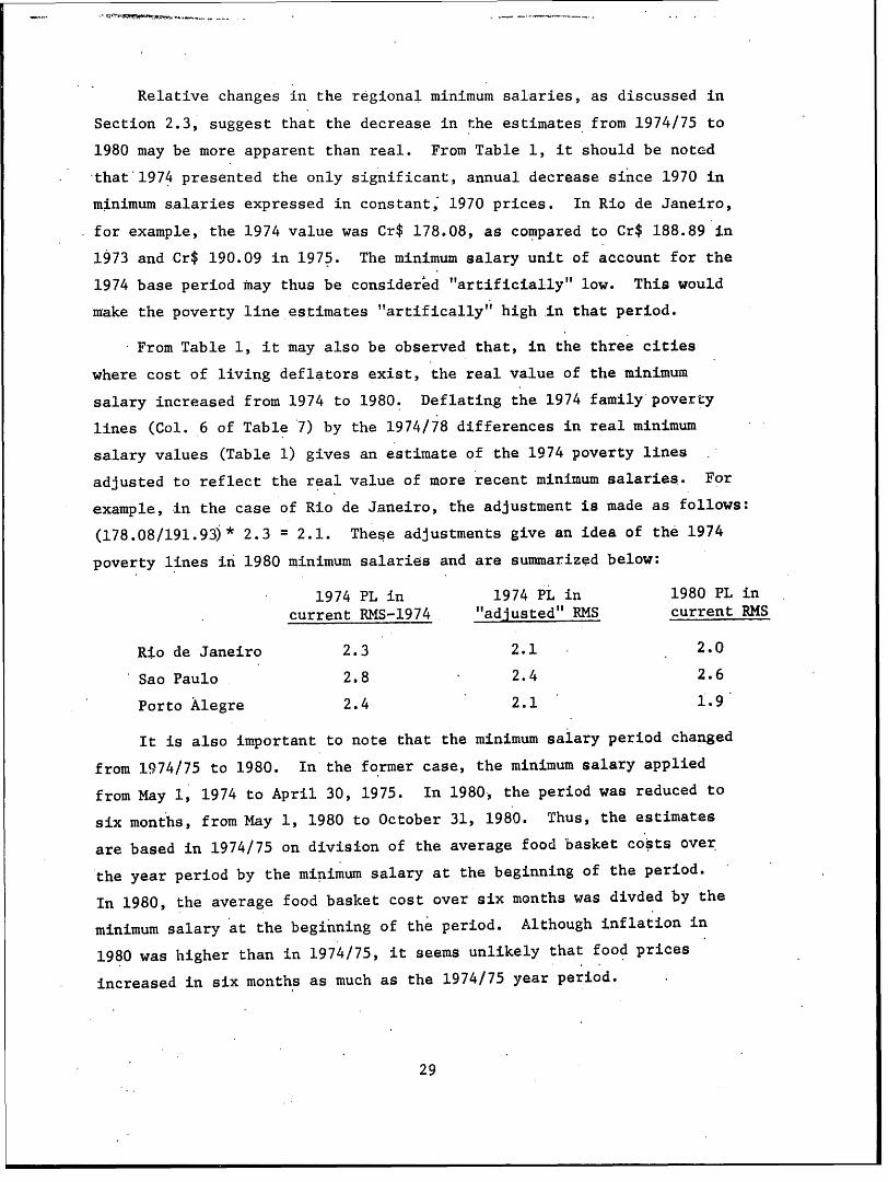
Relative changes in the regional minimum salaries, as discussed in
Section 2.3, suggest that the decrease in the estimates from 1974/75 to
1980 may be more apparent than real. From Table 1, it should be noted
*that 1974 presented the only significant, annual decrease since 1970 in
minimum salaries expressed in constant; 1970 prices. In Rio de Janeiro,
for example, the 1974 value was Cr$ 178.08, as compared to Cr$ 188.89 in
1973 and Cr$ 190.09 in 1975. The minimum salary unit of account for the
1974 base period may thus be considered "artificially" low. This would
make the poverty line estimates "artifically" high.in that period.
From Table 1, it may also be observed that, in the three cities
where cost of living deflators exist, the real value of the minimum
salary increased from 1974 to 1980. Deflating the 1974 family poverty
lines (Col. 6 of Table 7) by the 1974/78 differences in real minimum
salary values (Table 1) gives an estimate of the 1974 poverty lines
adjusted to reflect the real value of more recent minimum salaries. For
example, in the case of Rio de Janeiro, the adjustment is made as follows:
(178.08/191.93)* 2.3 = 2.1. These adjustments give an idea of the 1974
poverty lines in 1980 minimum salaries and are summarized below:
1974 PL in 1974 PL in 1980 PL incurrent RMS-1974. "adjusted" RMS current RMS
Rio de Janeiro 2.3 2.1 2.0
Sao Paulo 2.8 2.4 2.6
Porto Alegre 2.4 2.1 1.9
It is also important to note that the minimum salary period changed
from 1974/75 to 1980. In the former case, the minimum salary applied
from May 1, 1974 to April 30, 1975. In 1980, the period was reduced to
six months, from May 1, 1980 to October 31, 1980. Thus, the estimates
are based in 1974/75 on division of the average food basket costs over
the year period by the minimum salary at the beginning of the period.
In 1980, the average food basket cost over six months was divded by the
minimum salary 'at the beginning of the period. Although inflation in
1980 was higher than in 1974/75, it seems unlikely that food prices
increased in six months as much as the 1974/75 year period.
29
Another tendency noted (Table 2) is for the regional minimum salaries
to "converge" toward the highest regional figure. Columns 8 and 9 of
Table 7 show the impact of this tendency, with the poverty lines expressed
in units of the highest regional minimum salary of each period.
Although the available data often impose the use of the minimum
salary as a unit of account, the changes it has demonstrated often make
difficult interpretation of results. This suggests that periodic up-
dating of absolute, city-specific poverty line el;timates would be wise,
especially if more recent food basket weights and shares are developed.
One of the assumptions on which the 1980 estimates are based is
that relative food prices have not significantly changed from 1974/75 to
1980. This assumption was investigated through the use of linear regression
models, with the per capita poverty line estimates in 1974/75 and 1980
current cruzeiros (Columns 2.and 3 of Table 7) as the dependent variables.
The independent variables for each city were: median global family
expenditures in 1974 (which are negatively correlated with the s values);
population in-l975; population in 1980; and the food prices of the
minimum diet basket (see Table 5).
The most relevant results of the regression analysis are presented
in Table 8. They indicate that, although the fit of the models in the
two periods is quite good, the coefficients are not temporally stable.
This may be explained, in part, by Ehifts in relative prices.
Another indication that relative prices did not remain stable over
the observed periods is that factor analyses done with the food prices
for 1974/75 and 1980 generated factors with quite different structures
for each period.
Although our analysis indicates that each food item did not present
temporal price stability, we also investigated the possibility that the
basic diet price structure did not shift significantly. For this, a
"staple" portion of the diet was defined as five food items selected on
the basis of their, weights in the minimum diet cost (rice, black beans,
milk, bread and manioc flour). The methodology was tested through
30
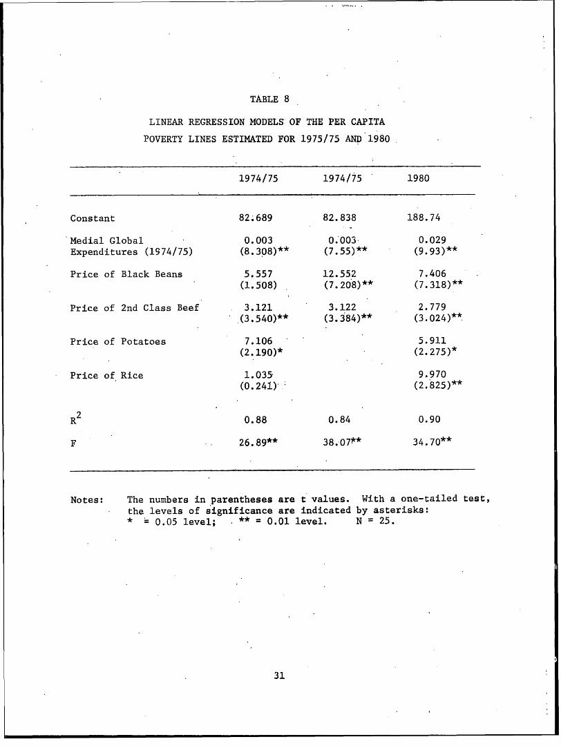
TABLE 8
LINEAR REGRESSION MODELS OF THE PER CAPITA
POVERTY LINES ESTIMATED FOR 1975/75 AND 1980
1974/75 1974/75 1980
Constant 82.689 82.838 188.74
Medial Global 0.003 0.003 0.029Expenditures (1974/75) (8.308)** (7.55)** (9.93)**
Price of Black Beans 5.557 12.552 7.406(1.508) (7.208)** (7.318)**
Price of 2nd Class Beef 3.121 3.1,22 2.779.(3.540)** (3.384)** (3.024)**
Price of Potatoes 7.106 5.911(2.190)* (2.275)*
Price of Rice 1.035 9.970(0.241); (2.825)**
R 0.88 0.84 0.90
F 26.89** 38.07** 34.70**
Notes: The numbers in parentheses are t values. With a one-tailed test,the levels of significance are indicated by asterisks:* 0.05 level; ** 0.01 level. N = 25.
31
predicting the 1980 minimum diet cost with data on cost of the staple
items in 1980 and the percent of total diet cost going to the staple
-items in 1974/75:
STAPLEEN]) 8
PSTAPLE7
where, EMD8 estimated per capita cost of the totalminimum diet in 1980;
STAPLE = cost of the staple food items in.1980;8PSTAPLE7 percent of total diet cost in 1974/75
allocated to the staple items
The results of this approach are presented in Table 9 and demonstrate.
that the staple share shifted less than might 'have been expected from
the individual food item regression coefficients. Thus, although the
price of each food item was not very stable over the period, the cumulative
price changes of the items within the staple share tended to have a
relatively stable net effect in most of the sample cities.
The mean of the ratio of predicted to observed minimum diet cost
(Col. 6 of Table 9) is 1.06, with a standard deviation of 0.10.and
coefficient of variability of 0.09. The greatest overestimate (27%)
occurred in Belo Horizonte; the largest underestimate (13%) in Porto
Velho. There was a less than 5% difference in predicted and observed
costs in 9 of the 25 cases.
The regression and staple share methodologies were also developed
in an attempt to identify an instrument for future calculations of
absolute poverty lines with readily available data, at a low cost and
with a reasonable degree of accuracy. The results indicate that the
staple. share approach is superior. In addition to decreasing the problem
of temporal price stability, the-share methodology also avoids the
problems of multi-colinearity and presents less demanding data requirement:se
32
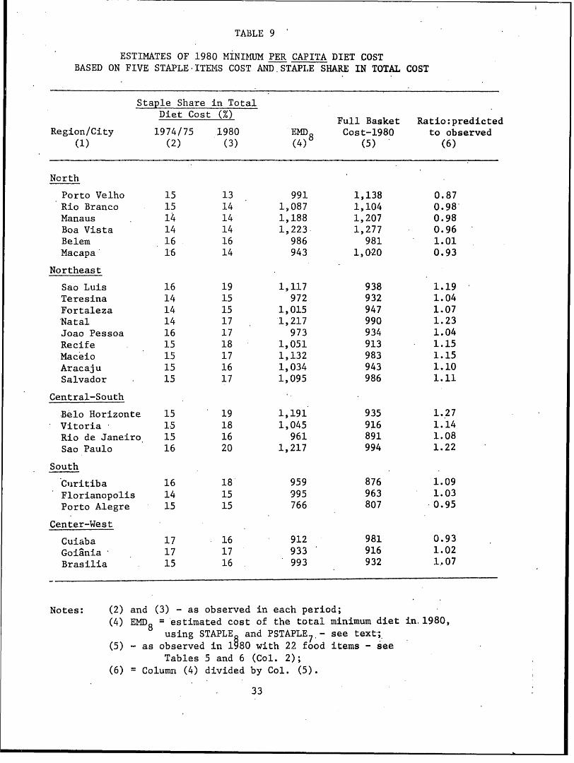
TABLE 9
ESTIMATES OF 1980 MINIMUM PER CAPITA DIET COST
BASED ON FIVE STAPLE ITEMS COST AND.STAPLE SHARE IN TOTAL COST
Staple Share in TotalDiet Cost ( Full Basket Ratio:predicted
Region/City 1974/75 1980 EMD8 Cost-1980 to observed
(1) (2) (3) (4) (5) (6)
North
Porto Velho 15 13 991 1,138 0.87
Rio Branco 15 14 1,087 1,104 0.98
Manaus 14 14 1,188 1,207 0.98
Boa Vista 14 14 1,223 1,277 0.96
Belem 16 16 986 981 1.01
Macapa' 16 14 943 1,020 0.93
Northeast
Sao Luis 16 19 1,117 938 1.19Teresina 14 15 972 932 1.04
Fortaleza 14 15 1,015 947 1.07
'Natal 14 17 1,217 990 1.23Joao Pessoa 16 17 973 934 1.04
Recife 15 18 1,051 913 1.15
Maceio 15 17 1,132 983 1.15
Aracaju 15 16 1,034 943 1.10
Salvador 15 17 1,095 986 1.11
Central-South
Belo Horizonte 15 19 1,191 935 1.27
Vitoria 15 18 1,045 916 1.14Rio de Janeiro 15 16 961 891 1.08
Sao Paulo 16 20 1,217 994 1.22
South
Cuiritiba 16 18 959 876 1.09Florianopolis 14 15 995 963 1.03Porto Alegre 15 15 766 807 0.95
Center-West
Cuiaba 17 16 912 981 0.93
Goiania 17 17 933 916 1.02Brasilia 15 16 993 932 1.07
Notes: (2) and (3) - as observed in each period;(4) EMD8 = estimated cost of the t.otal minimum diet in. 1980,
using STAPLE and PSTAPLE7, - see text;(5) - as observed in 1080 with 22 food items - see
Tables 5 and 6 (Col. 2);(6) = Column (4) divided by Col. (5).
33
4.3 Comparisons of Poverty Lines by City Size
Table 10 presents the major indicators of absolute poverty in 1974
and 1980, with averages for all the cities, and disaggregated averages
for the major size categories: metropolitan and non-metropolitan, or
medium-sized cities. Given the significantly higher cost of food in the
Northern cities, another category of medium-sized cities, excluding the
Northern region, was created.
Two counter-balancing effects on the poverty lines may be noted.
On one hand, differences in the cost of the minimum diet tended to
decrease over the period. The most expensive diet in 1974 (medium-sized
cities) had the smallest increase. The opposite occurred in the metro-
politan cities. This would tend to cause the poverty lines in the
metropolitan cities to increase relatively more than the medium-sized
cities over the period. The lower food share (s) values of metro-
politan cities tend to reinforce this tendency. On the other hand, the
changes in the minimum salary structure, as already discussed, with
convergence toward the highest national values, tended to off-set the
food cost difference on the poverty lines expressed in regional minimum
salaries. The net effect 4/ was to change rather significant city-size
differences in the family poverty lines in 1974 to essentially the same
figure for all categories in 1980.
4.4 Regional Comparisons of the Poverty Lines
.Table 11 presents an inter and intraregional perspective of the
poverty lines. Some of the general patterns discussed in the previous
-/Differences in s values are consistent with our knowledge ofBrazilian cities and location theory. In the metropolitan regions,families must spend relatively more of disposable income on non-fooditems than in smaller cities, particularly for land rent and/or trans-portation. Thus, in general, a family living in a metropolitan regionwith the same food expenditure as a family in a medium-sized city wouldrequire more income to have approximately the same level of welfare.
4/ The average family size differences are too small to merit muchdiscussion. However, the small difference in favor of smaller familiesin metropolitan regions tendsto complement the general trend described.
34
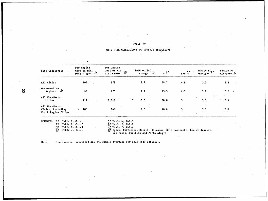
TABLE 10
CITY SIZE COMPARISONS OF POVERTY INDICATORS
Per Capita Per CapitaCity Categories Cost of Min. Cost of Min. 1974- 1980 Family PL Family Pi.Diet - 1974 - Diet -1980 - Change - S - AFS - RMS-1974 - RMS-1980 7/
All cities 106 979 9.2 48.2 4.9 3.5 2.8
Metropolitan 8/Regions - 925 9.7 43.5 4.7 3.1 2.7
All Non-Metro.Cities 112 1,010 9.0 50.8 5 3.7 2.9
All Non-Hetro.Cities, Excluding * 100 948 9.5 48.6 5 3.5 2.8North Region Cities
SOURCES: 1/ Table 6, Col.l 5/ Table 6, Col.62/ Table 6, Col.2 6/ Table 7, Col.63/ Table 6, Col.3 7/ Table 7, Col.74/ Table 7, Col.l 87 Belem, Fortaleza, Recife, Salvador, Belo Horizonte, Rio de Janeiro,
Sao Paulo, Curitiba and Porto Alegre.
NOTE: The figures presented are the simple averages for each city category.
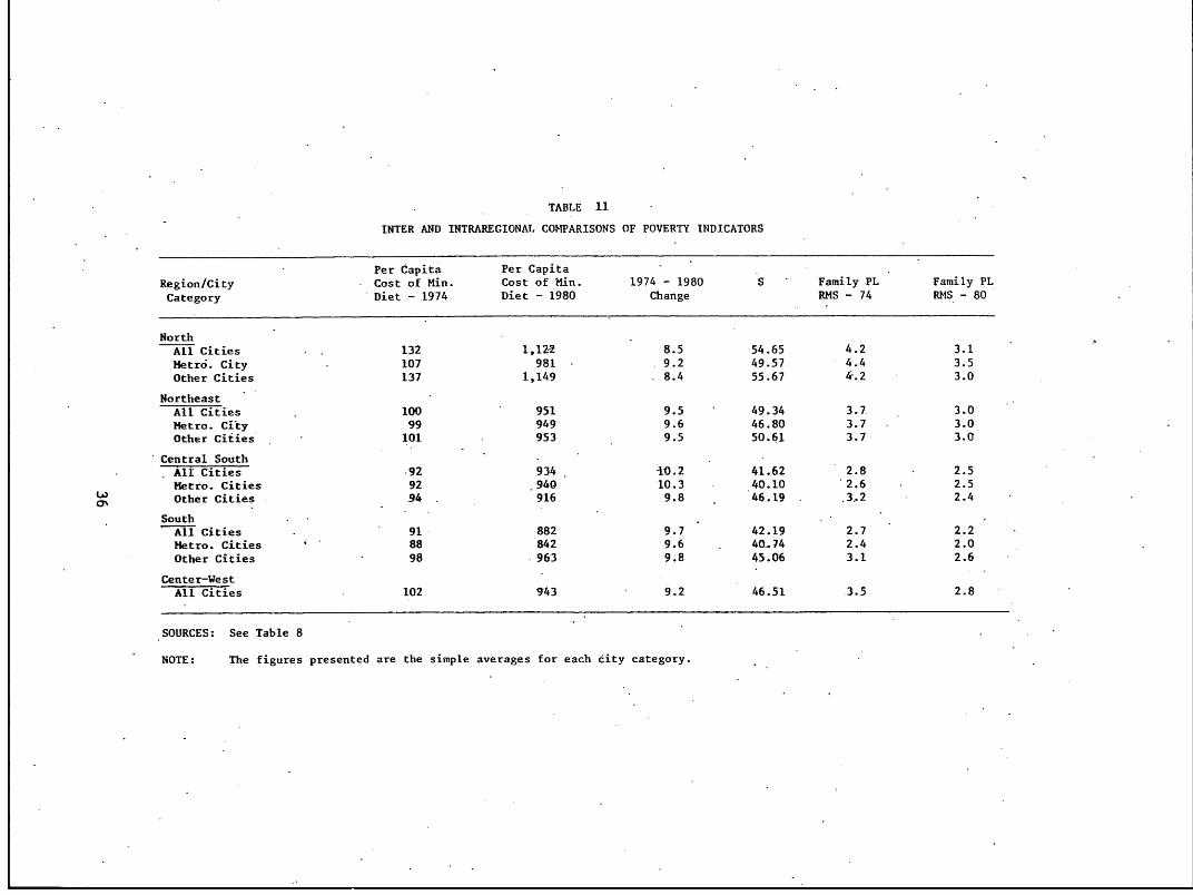
TABLE 11
INTER AND INTRAREGIONAL COMPARISONS OF POVERTY INDICATORS
Per Capita Per CapitaRegion/City - Cost of Min. Cost of Min. 1974 - 1980 S Family PL Family PLCategory Diet - 1974 Diet - 1980 Change RMS - 74 RMS - 80
NorthAll Cities - 132 1,12-2 8.5 54.65 4.2 3.1Metro. City 107 981 9.2 49.57 4.4 3.5Other Cities 137 1,149 8.4 55.67 4.2 3.0
NortheastAll Cities 100 951 9.5 49.34 3.7. 3.0Metro. Ci-ty 99 949 9.6 46.80 3.7 - 3.0Other Cities 101 953 9.5 50.61 3.7 3.C
Central SouthAll Cities -92 934 10.2 41.62 2.8 2.5Hetro. Cities 92 940 10.3 - 40.10 2.6 2.5Other Cities 94 916 9.8 46.19 .3.2 2.4
SouthAll Cities 91 882 9.7 42.19 2.7 2.2Metro. Cities 88 842 9.6 40-74 2.4 2.0Other Cities 98 963 9.8 45.06 3.1 2.6
Center-WestAll Cities 102 943 9.2 46.51 3.5 2.8
SOURCES: See Table 8
NOTE: The figures presented are the simple averages for each city category.
section apply here. For example, the food share (s) of the metropolitan
cities is lower than the s for other cities in all relevant regions.
The metropolitan city of the North had the lowest minimum diet cost in
1974, and the largest diet cost increase relative to Qther cities of theregion. However, differences in metropolitan versus non-metropolitan
diet costs were negligible in the Northeast, and the pattern was inverted
in the Central South and South.
The net effect on family poverty line estimates was to increase
within-region differences in the North over the period, decrease them in'
the Central South and to have an 'essentially neutral 'impact in the
Northeast and the South.
A comparison of the indicators persented in Tables 10 and 11 shows
that a substantial amount of intraregional differences in absolute
poverty line indicators by city size is lost when national aggregation
by city size is done.
Table 12 further examines internal intraregional differences in the
poverty'indicators. With the exception of the North Region, the amount
of variation between the cities within each of the five Macro-Regions is
'relatively low. The greater variation within the North is due to the
inclusion of Belem with the other capitals of the States and Territories
of the Amazon River Basin, where the cost of food is-quite high.
Considering the low number of observations, the F statistic is not
presented as a formal statistical test of the differences in population
means. Rather, it should be regarded as a rough indicator of how theratio of inter to intraregional variation in the per capita minimum diet
'costs and poverty line's changed over the period. In other words, it canbe seen as a measure of the ratio of the variation in the mean values of
these poverty indicators between the macro-regions to that within the
regions.. For both per capita diets and current cruzeiro poverty lines,
the ratio decreased from 1974/75 to 1980. Although these decreases are
not conclusive, they suggest that the interregional differences in food
costs may be decreasing over time. This is an especially important
potential trend to note because it is based on direct cost information
and is not influenced by food share, family size or minimum salary,
considerations.
37
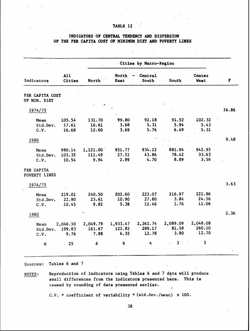
TABLE 12
INDICATORS OF CENTRAL TENDENCY AND-DISPERSIONOF THE PER CAPITA COST OF MINIMUM DIET AND POVERTY LINES
Cities by Macro-Region
All North - Central CenterIndicators Cities North East South South West F
PER CAPITA COSTOF MIN. DIET
1974/75 16.86
Mean 105.54 131.70 99.80 92.18 91.52 102.32Std.Dev. 17.61 16.61 3.68 5.31 5.94 5.43
C.V. 16.68 12.60 3.69 5.76 6.49 5.31
1980 9.48
Mean 980.14 1,121.00 951.77 934.22 881.94 942.95
Std.Dev. 103.35 111.49 27.51 43.86 78.42 33.63
C.V. 10.54 9.94 2.89 4.70 8.89 3.56
PER CAPITAPOVERTY LINES
1974/75 3.63
Mean 219.01 240.50 202.60 223.07 216.97 221.86Std.Dev. 22.90 23.61 10.90 27.80 3.84 24.56C.V. 10.45 9.82 5.38 12.46 1.76 11.06
1980 ' 2.36
Mean 2,046.50 2,049.79 1,933.47 2,262.74 2,089.09 2,048.08
Std.Dev. 199.83 161.67 122.82 289.17 81.58 260.10C.V. 9.76 7.88 6.35 12.78 3.90 12.70
N 25 6 9 4 3 3
Sources: Tables 6 and 7
NOTES: Reproduction of indicators using Tables 6 and 7 data will producesmall differences from the indicators presented here. This iscaused by rounding of data presented earlier.
C.V. = coefficient of variability = (std.dev./mean) x 100.
38
Perhaps even more important than this trend, however, is to observe
in Table 12 that the average per capita cost of the minimum diet is
highest in the pooLCr regions for both periods. This has significant
implications for evaluating the absolute poverty line estimates in terms
of the Bank's relative poverty standard and is a subject of the following
chapter.
39
5. COMPARISON OF ABSOLUTE AND RELATIVE POVERTY LINES AND EVALUATION OF RESULTS
An up-date of the World Bank's relative, urban poverty line is.
estimated in Annex I to be Cr$ 6,745 of monthly income for a family of
average size in 1979. The key question here is how to interpret this
figure: -what standard unit of account best interprets this cruzeiro
amount over time and between cities.
The current approach of the Bank is to standardize the cruzeiro,
figure through.use of the highest regional minimum salary as the unit of
account. This is assumed to be an indicator which is relatively stable
over time - , with regional differences in the cost of living accurately
reflected in the regional differences in the minimum salary.
The policy of the Brazilian government has been to establish the
highest regional minimum salary in the richer regions, the Central South
and South, and the lowest in the poorest region, the Northeast, with the2/
North and Center-West having intermediate level. - Estimates of the
per capita costs of the minimum diet (Table 12) indicate that the Bank's
assumption about regional differences in the minimum salary accurately
reflecting regional differences in the cost of living may not be valid.
With the exceptions of the North Region, and the Center-West in 1974/75,
the Northeast had the highest per capita cost of the nutritionally
adequate diet, and the South the lowest cost in both periods.
Our methodology is focused on absolute poverty indicators based on
a nutritional standard. Because the absolute poverty lines are estimated
from the food cost share of total family expenditures, we can make only
inferences about the non-food share of total expenditures. We can
conclude, however, that to the extent our minimum cost, nutritionally
adequate food basket is accurately defined and weighted, and valid over
time and between cities, then the cost of a nutritionally adequate diet
has been and continues to be greater in the poorer regions with lower
l/ The assumed temporal stability has been verified, at least over
the last five years.
2/-/Current exceptions are Recife and Salvador of the Northeast
having a middle-level regional minimum salary and the Center-West's
Brasilia having the highest level.
40
regional minimum slaries. Unless the non-food expenditures are substan-
tially less in the poor cities, the assumption about regional minimum
slaries accurately reflecting cost of living differences is not valid..
This study's scope did not permit-direct analysis of non-food
expenditures. The food share estimate of total expenditures is based on
the observed share in the expenditure interval closest to the Bank's
relative poverty line of each ENDEF region in 1974/75. An up-dating of
food and non-food shares would be a valuable complement to the presentstudy.
Table 13 presents a regional summary of the absolute and relative
poverty line estimates.. With current criteria, the Bank's relative
standard is three regional minimum salaries in all cities of all regions.As a basis of comparison, the relative poverty line estimate in cruzeirosis also expressed in units of the relevant regional minimum salary.Because of the trend to reduce the number of minimum salaries, the
absolute estimates are also presented in units of the highest minimum
salary.
In the 1974/75 period, the absolute estimates expressed in RMS are
higher than the relative standard of three HMS in the North and Northeast.
When the relative estimate is expressed in RMS, this occurs only in thecase of the North. In 1980, relative estimates expressed in both HMS
and RMS are higher than the absolute estimates expressed in RMS, with
slight exceptions in the North and Northeast. As discussed earlier,
changes in the regional minimum salary levels make interpretation ofthese figures difficult.
Table 14 attempts to facilitate this interpretation through presenting
the ratios of the absolute estimates to the relative estimates. One way
of interpreting the ratios is that the higher the ratio, the greater
the risk of excluding poor people from the target group.. A relatively
lower ratio presents the risk of including non-poor in the group.
Another way of interpreting the ratios is that less distortions in the
application of the Bank's relative poverty criterion should result when
the ratios vary little between regions.
41
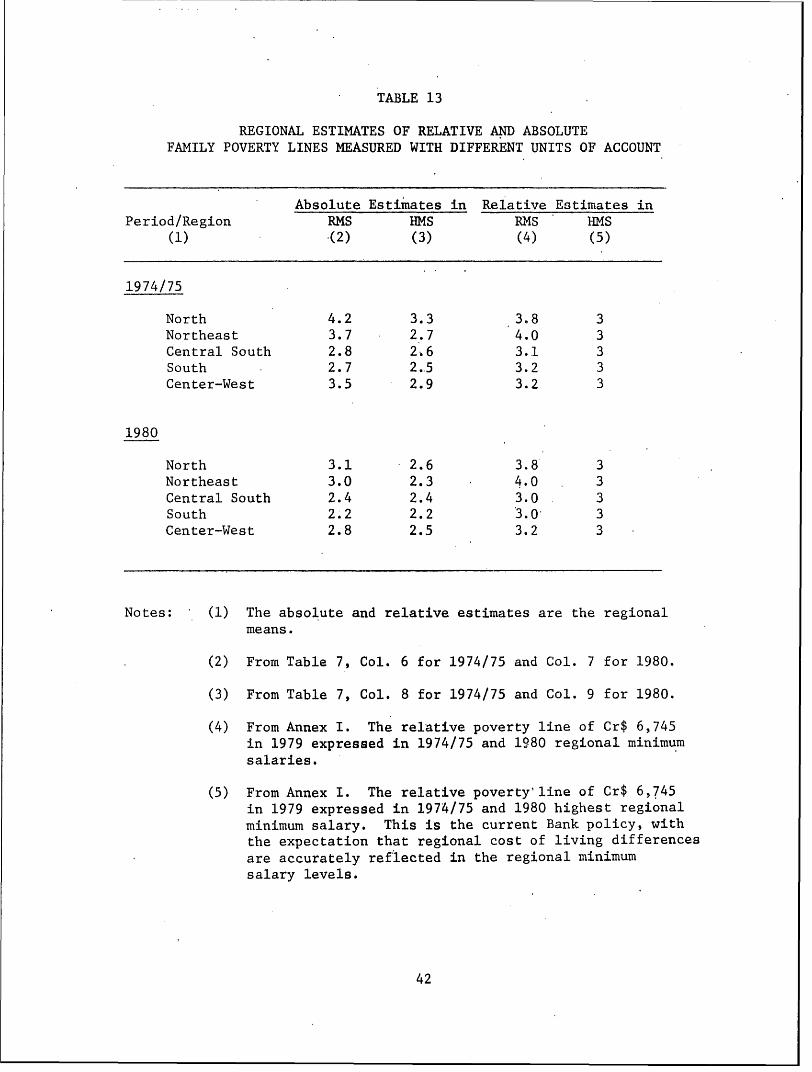
TABLE 13
REGIONAL ESTIMATES OF RELATIVE AND ABSOLUTEFAMILY POVERTY LINES MEASURED WITH DIFFERENT UNITS OF ACCOUNT
Absolute Estimates in Relative Estimates inPeriod/Region RMS HMS RMS HMS
(1) *(2) (3) (4) (5)
1974/75
North 4.2 3.3 3.8 3Northeast 3.7 2.7 4.0 3Central South 2.8 2.6 3.1 3South 2.7 2.5 3.2 3Center-West 3.5 2.9 3.2 3
1980
North 3.1 2.6 3.8 3Northeast 3.0 2.3 4.0 3Central South 2.4 2.4 3.0 3South 2.2 2.2 3.0 3Center-West 2.8 2.5 3.2 3
Notes: (1) The absolute and relative estimates are the regionalmeans.
(2) From Table 7, Col. 6 for 1974/75 and Col. 7 for 1980.
(3) From Table 7, Col. 8 for 1974/75 and Col. 9 for 1980.
(4) From Annex I. The relative poverty line of Cr$ 6,745in 1979 expressed in 1974/75 and 1980 regional minimumsalaries.
(5) From Annex I. The relative poverty'line of Cr$ 6,745in 1979 expressed in 1974/75 and 1980 highest regionalminimum salary. This is the current Bank policy, withthe expectation that regional cost of living differencesare accurately reflected in the regional minimumsalary levels.
42
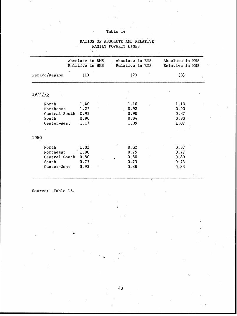
Table 14
RATIOS OF ABSOLUTE AND RELATIVEFAMILY POVERTY LINES
Absolute in RMS Absolute in RMS Absolute in HMSRelative in HMS Relative in RMS Relative in HMS
Period/Region (1) (2) (3)
1974/75
North 1.40 1.10 1.10Northeast 1.23 0.92 0.90Central South 0.93 0.90 0.87South 0.90 0.84 0.83Center-West 1.17 1.09 1.07
1980
North 1.03 0.82 0.87Northeast 1.00 0.75 0.77Central South 0.80 0.80 0.80South 0.73 0.73 0.73Center-West 0.93 0.88 0.83
Source: Table 13.
43
Column 1 of Table 14 presents an evaluation of the current Bank
policy to express the relative poverty line in terms of the highest
regional minimum salary. Although the range of the ratio values decreased
from 1974/75 to 1980, the risk of excluding the poor remains highest in
the North and Northeast and the risk of including non-poor is greater in
the South in both periods.
If the normative interpretations of the ratios are correct, Column
2 presents a superior application of the Bank's relative poverty criterion.
The range of the ratio values is less in both periods when compared to
Column 1, and the poorest region, the Northeast, has less risk of having
its poor excluded from the benefits of Bank financed projects.
Column 3 of Table 14 presents an evaluation of what may happen: an
evolution to one, national minimum salary. Comparison of this column's
ratios to those of Column 1 indicates that the trend to less regional
variation in the minimum salary should decrease the potential risks of
the current application of the Bank's relative poverty standard.
The major conclusion of this study is that an evaluation of the
application of the Bank's relative poverty criterion through estimates
of absolute poverty lines indicates that the use of regional minimum
salaries in translTaing the national, urban relative poverty line in
cruzeiros to minimum salary units would decrease the risks of bias in
urban project design and appraisal. Specifically, this recommendation
means that the Bank would better evaluate the poverty impact of its
projects by substituting the standard of three regional minimum salaries
in all cities with three regional minimum salaries in the cities of the
Central South, South and Brasilia, and four regional minimum salaries in
the cities of the North, Northeast, Cuiaba and Goiania.
The impact of this recommendation in terms of the number of families
considered to be in the urban poverty target group is presented in
Tables 15-18. For these tables, Annex III data were used. There, a
series of tables presents the size distribution of family expenditures
for the 15 ENDEF regions uised in this study. These tables permit an
estimate of the percentage of families with expenditures less than the
poverty lines according to the various criteria. These estimates are
44
not precise, because families are grouped by expenditure intervals and
linear interpolation, of course, is not very accurate. They should,
however, provide an acceptable "order of magnitude" useful for comparison
of the impacts of the diffirent criteria.
Table 18 demonstrates that the recommended change in application of
the Bank's relative poverty criterion would result in a slight (approximately
3%) increase in the percent-age of urban.families considered poor in the
25 cities surveyed.
The overall impact of the recommended change in the relative poverty
criterion application is relatively small, of course, because of the
large number of families in the Central South and South regions, where
no change is recommended. Operationally,. the recommendation would mean
that some 280 thousand families of the North, Northeast,. and Cuiaba and
Goiania would be considered poor, while under the current application
of the criterion they would not be considered poor. The recommended
change would decrease the risk of excluding poor families from the
target group, while, of course, increasing the risk of including the
non-poor.
Other considerations of estimating the poverty lines, especially
variations in family size, monetary versus non-monetary income and use
of the "behavioral" diet, are presented in Annex IV.
45
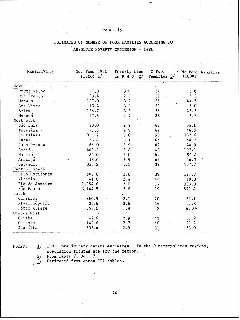
TABLE 15
ESTIMATES OF NUMBER OF POOR FAMILIES ACCORDING TO.
ABSOLUTE POVERTY CRITERION - 1980
Region/City No. Fam. 1980 Poverty Line % Poor No.Poor Families(1000) 1/ in R M S 2/ Families 3/ (1000)
NorthPorto Velho 27.0 3.0 32 8.6Rio Branco 23.4 2.9 31 7.3Manaus 127.0 3.2 35 44.5Boa Vista 13.4 3.3 37 5.0Belem 166.7 3.5 26 43.3Macapa 27.6 2.7 28 7.7
NortheastSao Luis 90.0 2.9 62 55.8Teresina 75.6 2.9 62 46.9Fortalez.a. 316.2 3.0 53 167.6Natal 83.4 3.1 65 54.2Joao Pessoa 66.0 2.9 62 40.9Recife 469.2 2.8 42 197.1Macei6 80.0 3.0 63 50.4Aracaju 58.6 2.9 62 36.3Salvador 353.2 3.3 39 137.7
Central SouthBelo Horizonte 507.0 2.8 39 197.7Vit6ria 41.6 2.4 44 18.3Rio de Janeiro 2,254.8 2.0 17 383.3Sao Paulo 3,144.5 2.6 19 597.4
SouthlCuritiba 360.5 2.1 20 72.1Florianopolis 37.6 2.6 34 12.8Porto Alegre 558.0 1.9 12 67.0
Center-W4estCuiaba 42.6 2.9 42 17.9Goiania 143.6 2.7 40 57.4Brasilia 235.4 2.9 31 73.0
NOTES: 1/ IBGE, preliminary census estimates. In the 9 metropolitan regions,population figures are for the region.
2/ From Table 7, Col. 7.3/ Estimated from Annex III tables.
46
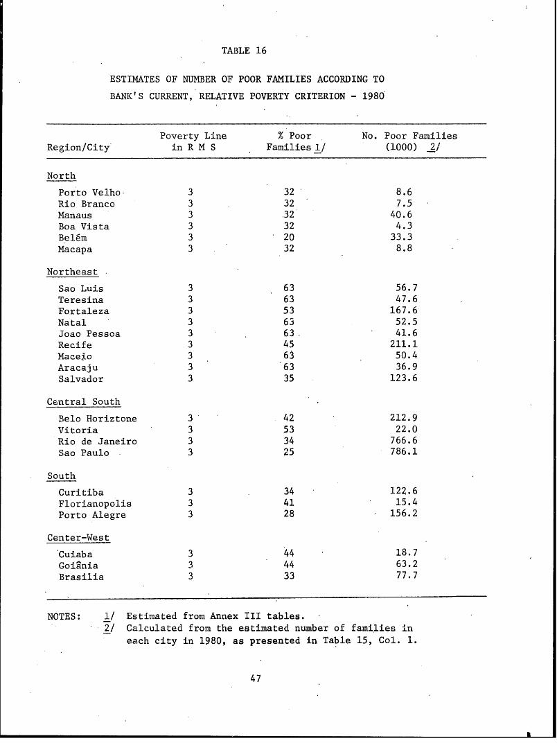
TABLE 16
ESTIMATES OF NUMBER OF POOR FAMILIES ACCORDING TO
BANK'S CURRENT, RELATIVE POVERTY CRITERION - 1980
Poverty Line % Poor No. Poor FamiliesRegion/City in R M S Families 1/ (1000) 2/
North
Porto Velho 3 32 8.6Rio Branco 3 . 32 7.5Manaus 3 .32 40.6Boa Vista 3 32 4.3Belem 3 20 33.3Macapa 3 32 8.8
Northeast
Sao Luis 3 63 56.7Teresina 3 63 47.6Fortaleza 3 53 167.6Natal 3 63 52.5Joao Pessoa 3 63. 41.6Recife 3 45 211.1Mace4o 3 63 50.4Aracaju 3 63 36.9Salvador 3 35 123.6
Central South
Belo Horiztone 3 42 212.9Vitoria 3 53 22.0Rio de Janeiro 3 34 766.6Sao Paulo . 3 25 786.1
South
Curitiba 3 . 34 122.6Florianopolis 3 41 15.4Porto Alegre 3 28 156.2
Center-West
Cuiaba 3 44 18.7Goiania 3 44 63.2Brasilia 3 33 77.7
NOTES: 1/ Estimated from Annex III tables.2/ Calculated from the estimated number of families in
each city in 1980, as presented in Table 15, Col. 1.
47
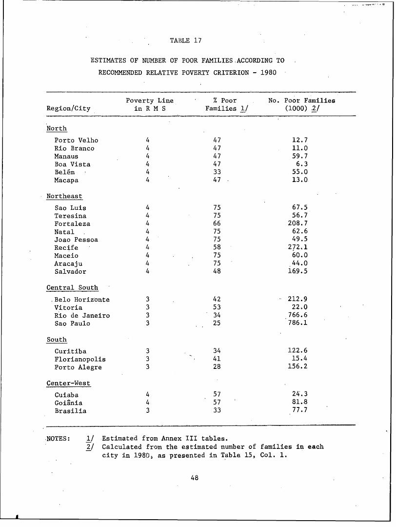
TABLE 17
ESTIMATES OF NUMBER OF POOR FAMILIES-ACCORDING TO
RECOMMENDED RELATIVE POVERTY CRITERION - 1980
Poverty Line % Poor No. Poor Families
Region/City in R M S Families 1/ (1000).2/
North
Porto Velho 4 47 12.7
Rio Branco 4 47 11.0
Manaus 4 47 59.7
Boa Vista 4 47 6.3
Belem 4 33 55.0
Macapa 4 47 13.0
Northeast
Sao Luis 4 75 67.5Teresina 4 75 56.7
Fortaleza 4 66 208.7
Natal . 4 75 62.6
Joao Pessoa 4 75 49.5Recife 4 58 272.1
Maceio 4 75 60.0
Aracaju 4 . 75 44.0
Salvador 4 48 169.5
Central South
Belo Horizonte 3 42 212.9
Vitoria 3 53 22.0
Rio de Janeiro 3 34 766.6
Sao Paulo 3 25 786.1
South
Curitiba 3 34 122.6
Florianopolis 3 41 15.4Porto Alegre 3 28 156.2
Center-West
Cuiaba 4 57 24.3
Goiania 4 57 81.8
Brasilia 3 33 77.7
NOTES: 1/ Estimated from Annex III tables.2/ Calculated from the estimated number of families in each
city in 1980, as presented in Table 15, Col. 1.
48
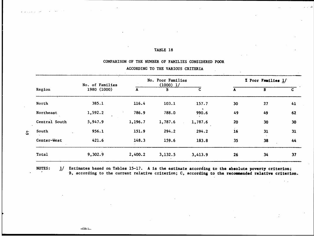
TABLE 18
COMPARISON OF THE NUMBER OF FAMILIES CONSIDERED POOR
ACCORDING TO THE VARIOUS CRITERIA
No. Poor Families Z Poor Faailies 1/No. of Families (1000) 1/ .
Region 1980 (1000) A B C A B C
North 385.1 116.4 103.1 157.7 30 27 41
Northeast 1,592.2 786.9 788.0 990.6 49 49 62
Central South 5,947.9 1,196.7 1,787.6 1,787.6 20 30 30
South 956.1 151.9 294.2 294.2 16 31 31
Center-West 421.6 148.3 159.6 183.8 35 38 44
Total 9,302.9 2,400.2 3,132.5 3,413.9 26 34 37
NOTES: 1/ Estimates based on Tables 15-17. A is the estimate according to the absolute poverty criterion;-*B, according to the current relative criterion; C, according to the reco,ended relative criterion.
-.
BIBLIOGRAPHY
Andre, Paulo T. A. de. "The Brazil 1974/75 National Household ExpenditureSurvey." Conducting Surveys in Developing Countries: PracticalProblems and Experiences in Brazil, Malaysia and The Philippines.Washington, D.C.: The World Bank Living Standards MeasurementsStudy Working Paper No. 5, 1980.
Beckerman, Wilfred. "The Measurement of Poverty in the Context of theWorld Bank's Activities." Washington, D.C.: World Bank Consultant'sReport, March 1981.
Conjuntura Economica. Vol. 33 No. 11 and Vol. 34, No. 12.
Davis, Ted J. and Alastair J. Stone. "Updating Poverty Income Levels."Washington, D.C.: The World Bank, Office Memorandum to CountryEconomists, July 7, 1978.
Fundacao Getulio Vargas. Dietas de Custo Minimo: Aplicacao daProgramacao Linear a Alimentacas Humana. Rio de Janeiro: FutdacaoGetulio Vargas, 1978.
Pesquisa sobre Consumo Alimentar. Rio de Janeiro:Fundacao Getulio Vargas, 1978.
Fundacao Instituto Brasileiro de Geografia e Estatistica - IBGE.Estudo Nacional de Despesas Familiares. Rio de Janeiro:IBGE, 1978. Unplublished data also used.
Indicadores Sociais - Relatorio 1979. Rio de Janeiro:IBGE, 1979.
Inquerito Nacional de Precos: Generos Alimenticios.Rio de Janeiro: IBGE, 1974-75; 1980.
Pesquisa Nacional por Amostra de Domicilios - 1976.Rio de Janeiro: IBGE, 1978.
Sinopse Preliminar do Censo Demografico - 1980: Brasil.Rio de Janeiro: IBGE, 1981.
Goedhart, Theo, et al. "The Poverty Line: Concept and Measurement."The Journal of Human Resources. Vol. 12.
Kuznets, Simon. "Demographic Aspects of Size Distribution oi Income:An Exploratory Essay." Economic Development and Cultural Change.Vol. 25 (October 1975).
Musgrove, Philip. "Household Size and Composition, Employment and Povertyin the Urban Latin America." Economic Development and Cultural Change.Vol. 28 (January 1980).
50
Orshansky, Mollie. "How Poverty is Measured." National Labor Review(February 1969).
Pfeffermann, Guy P. and Richard Webb. The Distribution of Income inBrazil. Washington, D.C.: The World Bank Staff Working PaperNo. 356. September 1979.
Sen, Amartya. "Issues in the Measurement of Poverty." ScandanavianJournal of Economics. Vol. 81 (1979).
Levels of Poverty: Policy and Change. Washington, D.C.:The World Bank Staff Working Paper No. 401. July 1980.
Thomas, Vinod. "Spatial Differences in Poverty: The Case of Peru."Journal of Development Economics. Vol. 7 (1980).
"Differences in Income, Nutrition and Poverty within Brazil."Washington, D.C.: The World Bank, Draft Copy (September 1981).
World Bank. Brazil: Human Resources Special Report. Washington, D.C.:The World Bank, 1979.
51
ANNEX I - 1979 ESTIMATES OF URBAN POVERTY LINES IN BRAZIL ACCORDING TO
WORLD BANK GUIDELINES
This annex seeks to update urban poverty line estimates for Brazil,
using World Bank guidelines and criteria. -/ The latest national accounts
and population estimates available are for 1979. A poverty line is
understood to mean the level of family income below which a family may
be considered poor. A poverty line is necessary to estimate the extent
to which benefits of Bank-financed projects will be channeled as directly
as possible to the urban poverty target group.
Classified as a "middle-income country", Brazil's urban poverty
target group is defined through the concept of relative poverty, in
which the target threshold, or poverty line, is calculated as one-third
of the national per capita income,.adjusted for urban-rural price
differences.2/ Operationally, the Bank's urban poverty line has been
calculated at the national level in minimum salary units. The minimum
salary is defined by law in Brazil and is the unit of account for many
income statistics. Currently, each Municipality is classified as belonging
to one of three minimum salary levels. -/ Thus, the Bank presently uses
a single urban poverty line, with expectation that regional differences
in the cost of living are accurately reflected by the regionally differentiated
minimum salary.
A rather detailed record of the calculations used in estimating
1979 poverty line is presented below. When relevant, data Adentification
in the original Portuguese is included in parentheses to facilitate the
identification of our data sources. These details are included in order
to make possible as precise comparisions as possible of the estimates
presented here with former ones, or future updates.
l/Bank guidelines and criteria are taken from Office Memorandum to
country economists from Messrs. Ted J. Davis and Alastair J. Stone: Subject -
"Updating Poverty Income Levels," Date - July 7, 1978. Especially,Attachment 5, Page 5.
2/ Ibid. Also, Wilfred Beckerman, "The Measurement of Poverty in the
Context of the World Bank's Activities," (Washington, D.C.: World Bank
Consultant's Report, March 1981), pp. 4-5.
3 The highest minimum salaries apply to the South and Southeast
regions; an intermediate level is established for most of the frontier(Central-West and Amazon regions), except Brasilia; the lowest level
applies to most of the Northeast, with the major exceptions of Recifeand Salvador, which have an intermediate level minimum salary.
52
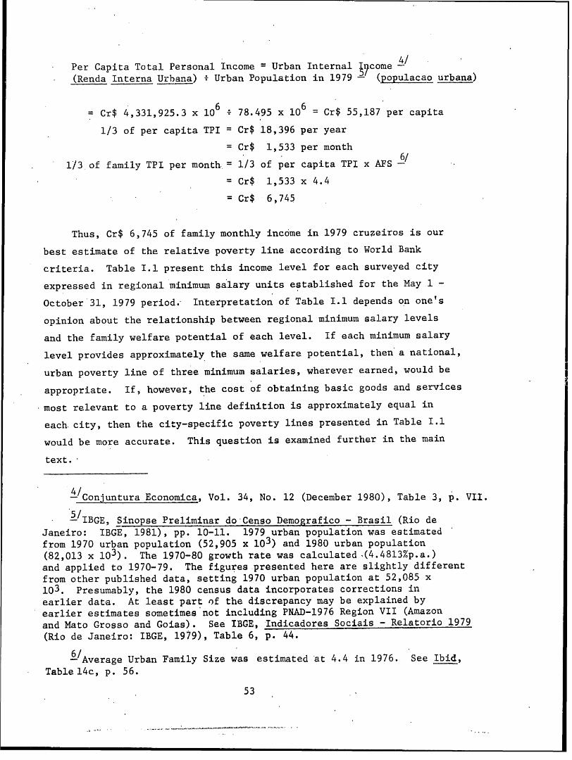
Per Capita Total Personal Income = Urban Internal come -
(Renda Interna Urbana) + Urban Population in 1979 - (populacao urbana)
C Gr$ 4,331,925.3 x 10 * 78.495 x 106 = Cr$ 55,187 per capita
1/3 of per capita TPI = Cr$ 18,396 per year
= Cr$ 1,533 per month
1/3 of family TPI per month. = 1/3 of per capita TPI x As
= Cr$ 1,533 x 4.4
= Cr$ 6,745
Thus, Cr$ 6,745 of family monthly income in 1979 cruzeiros is our
best estimate of the relative poverty line according to World Bank
criteria. Table I.1 present this income level for each surveyed city
expressed in regional minimum salary units established for the May 1 -
October 31, 1979 period. Interpretation of Table I.1 depends on one's
opinion about the relationship between regional minimum salary levels
and the family welfare potential of each level. If each minimum salary
level provides approximately the same welfare potential, then a national,
urban poverty line of three minimum salaries, wherever earned, would be
appropriate. If, however, the cost of obtaining basic goods and services
most relevant to a poverty line definition is approximately equal in
each city, then the city-specific poverty lines presented in Table I.1
would be more accurate. This question is examined further in the main
text.
4/Conjuntura Economica, Vol. 34, No. 12 (December 1980), Table 3, p. VII.
5-/IBGE, Sinopse Preliminar do Censo Demografico - Brasil (Rio de
Janeiro: IBGE, 1981), pp. 10-11. 1979 urban population was estimated
from 1970 urban population (52,905 x 103) and 1980 urban population
(82,013 x 103). The 1970-80 growth rate was calculated.(4.4813%p.a.)and applied to 1970-79. The figures presented here are slightly different
from other published data, setting 1970 urban population at 52,085 x
103. Presumably, the 1980 census data incorporates corrections in
earlier data. At least part of the discrepancy may be explained by
earlier estimates sometimes not including PNAD-1976 Region VII (Amazon
and Mato Grosso and Goias). See IBGE, Indicadores Sociais - Relatorio 1979
(Rio de Janeiro: IBGE, 1979), Table 6, p. 44.
6/Average Urban Family Size was estimated at 4.4 in 1976. See Ibid,
Table 14c, p. 56.
53
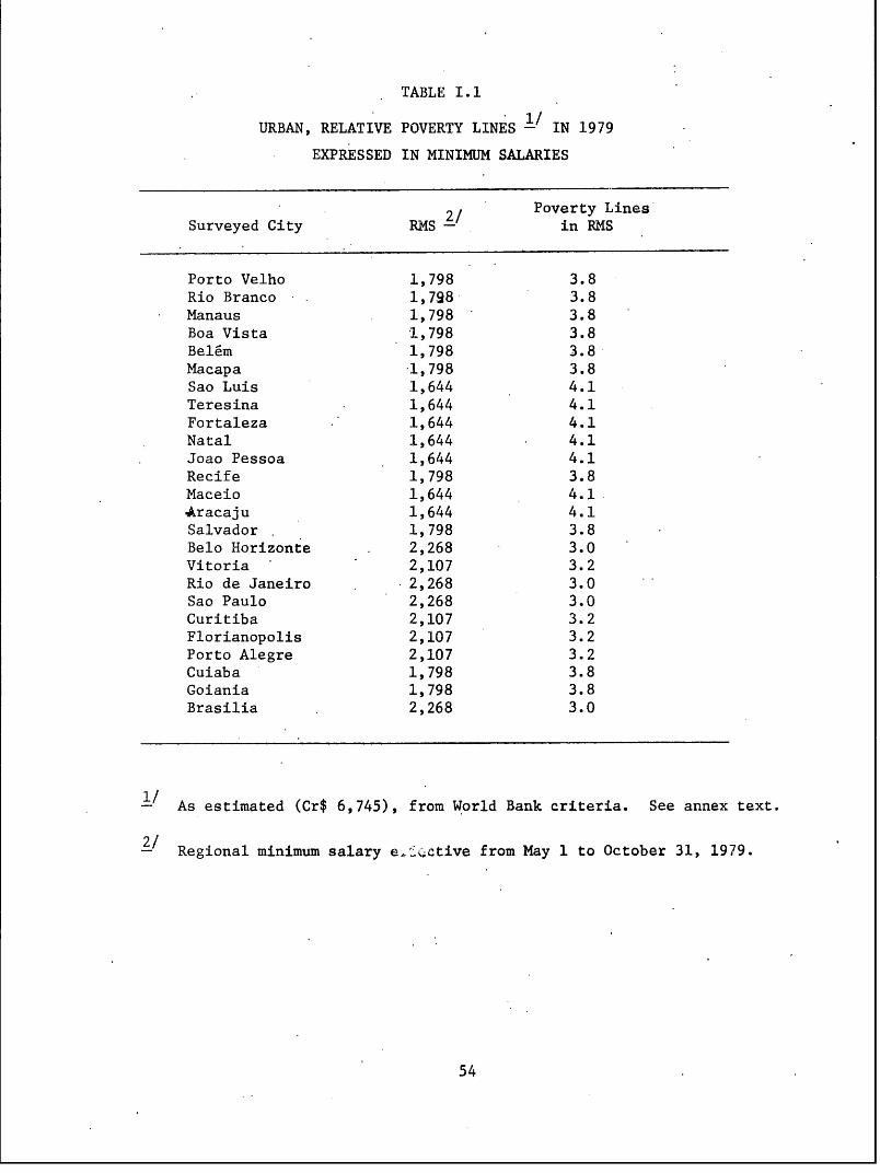
TABLE I.1
1/URBAN, RELATIVE POVERTY LINES - IN 1979
EXPRESSED IN MINIMUM SALARIES
2/ Poverty LinesSurveyed City RMS - in RMS
Porto Velho 1,798 3.8Rio Branco 1,798 3.8Manaus 1,798 3.8Boa Vista 1,798 3.8Belem 1,798 3.8Macapa 1,798 3.8Sao Luis 1,644 4.1Teresina 1,644 4.1Fortaleza 1,644 4.1Natal 1,644 4.1Joao Pessoa 1,644 4.1Recife 1,798 3.8Maceio 1,644 4.1,Aracaju 1,644 4.1Salvador 1,798 3.8Belo Horizonte 2,268 3.0Vitoria 2,107 3.2Rio de Janeiro 2,268 3.0Sao Paulo 2,268 3.0Curitiba 2,107 3.2Florianopolis 2,107 3.2Porto Alegre 2,107 3.2Cuiaba 1,798 3.8Goiania 1,798 3.8Brasilia 2,268 3.0
- As estimated (Cr$ 6,745), from World Bank criteria. See annex text.
- Regional minimum salary e'-ective from May 1 to October 31, 1979.
54
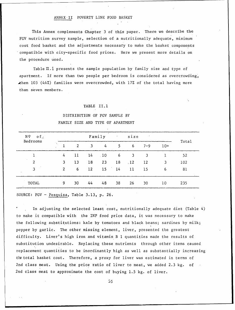
ANNEX II POVERTY LINE FOOD BASKET
This Annex complements Chapter 3 of this paper. There we describe theFGV nutrition survey sample, selection of a nutritionally adequate, minimumcost food basket and the adjustments necessary to make the basket componentscompatible with city-specific food prices. Here we present more details onthe procedure used.
Table 11.1 presents the sample population by family size and type ofapartment. If more than two people per bedroom is considered as overcrowding,then 103 (44%) families were overcrowded, with 17% of the total having morethan seven members.
TABLE II.1
DISTRIBUTION OF FGV SAMPLE BY
FAMILY SIZE AND TYPE OF APARTMENT
N9 of,; Family size*Bedrooms
Total1 2 3 4 5 6 7-9 10+
1 4 11 14 10 6 3 3 1 522 3 13 18 23 18 .12 12 3 1023 2 6 12 15 14 11 15 6 81
TOTAL 9 30 44 48 38 26 30 10 235
SOURCE: FGV - Pesquisa, Table 3.13, p. 26.
In adjusting the selected least cost, nutritionally adequate diet (Table 4)to make it compatible with the INP food price data, it was necessary to makethe following substitutions: kale by tomatoes and black beans; sardines by milk;pepper by garlic. The other missing element, liver, presented the greatestdifficulty. Liver's high iron and vitamin B 1 quantities made the results ofsubstitution undesirable. Replacing these nutrients through othdr items causedreplacement quantities to be inordinantly high as well as substantially increasingtlv total basket cost. Therefore, a proxy for liver was estimated in terms of2nd class meat. Using the price ratio of liver to meat, we added 2.3 kg. of2nd class meat to approximate the cost of buying 1.5 kg. of liver.
rL-
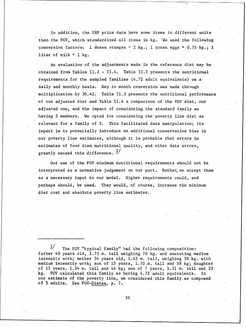
In addition, the INP price data have some items in different units
than the FGV, which standardized all items in kg. We used the following
conversion factors: 1 dozen oranges = 2 kg.; 1 dozen eggs = 0.75 kg.; 1
liter of milk = 1 kg.
An evaluation of the adjustments made in the reference diet may be
obtained from Tables II.2 - II.4. Table II.2 presents the nutritional
requirements for the sampled families (4.72 adult equivalents) on a
daily and monthly basis. Day to month conversion was made through
multiplication by 30.42. Table II.3 presents the nutritional performance
of our adjusted diet and Table II.4 a comparison of the FGV diet, our
adjusted one, and the impact of considering the standard family as
having 5 members. We opted for considering the poverty line diet as
relevant for a family of 5. This facilitated data manipulation; its
impact is to potentially'introduce an additional conservative bias in
our poverty line estimates,- although it is probable that errors in
estimates of food item nutritional quality, and other data errors,
greatly exceed this'difference. 1/
Our use of the FGV minimum nutritional requirements should not be
interpreted as a normative judgement on our part. Rather,we accept them
as a necessary input to our model. Higher requirements could, and
perhaps should, be used. They would, of course, increase the minimum
diet cost and absolute poverty line estimates.
1/ The FGV "typical family" had the following composition:
father 40 years old, 1.73 m. tall weighing 70 kg. and executing medium
intensity work; mother 34 years old, 1.63 m. tall, weighing 58 kg. with
medium intensity work; son of 15 years, 1.70 m. tall and 59 kg; daughter
of 13 years, 1.54 m. tall and 44 kg; son of 7 years, 1.21 m. tall and 23
kg. FGV calculated this family as having 4.72 adult equivalents. In
our estimate of the poverty line, we considered this family as composed
of 5 adults. See FGV-Dietas, p. 7.
56
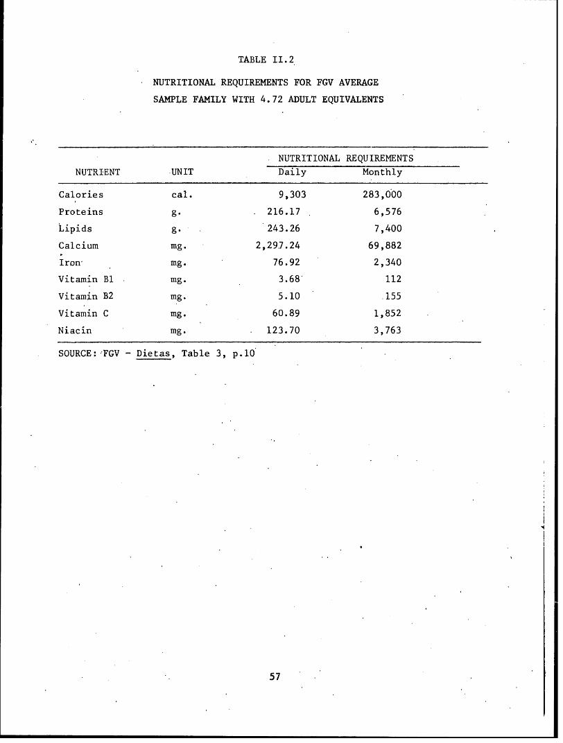
TABLE II.2
NUTRITIONAL REQUIREMENTS FOR FGV AVERAGE
SAMPLE FAMILY WITH 4.72 ADULT EQUIVALENTS
NUTRITIONAL REQUIREMENTS
NUTRIENT UNIT Daily Monthly
Calories cal. 9,303 283,000
Proteins g. 216.17 6,576
Lipids g. - 243.26 7,400
Calcium mg. 2,297.24 69,882
Iron' mg. 76.92 2,340
Vitamin Bl mg. 3.68 112
Vitamin B2 mg. 5.10 .155
Vitamin C mg. 60.89 1,852
Niacin mg. 123.70 3,763
SOURCE: FGV - Dietas, Table 3, p.1 0
57
57
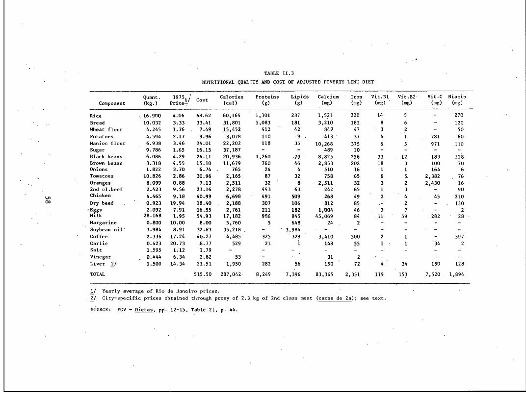
TAI3LE II.3
NUTRITIONAL QUALITY AND COST OF ADJUSTED POVERTY LINE DIET
Quant. 1975 Calories Proteins Lipids Calcium Iron Vit.B1 Vit.B2 Vit.C NiacinComponent (kg.) Price/ Cost (cal) (g) (g) (mg) (mg) (mg) (mg) (mg) (mg)
Rice 16.900 4.06 68.62 60,164 1,301 237 1,521 220 14 5 - 270
Bread 10.032 3.33 33.41 31,801 1,083 181 3,210 181 8 6 - 120
Wheat flour 4.245 1.76 7.49 15,452 412 42 849 47 3 2 - 50
Potatoes 4.594 2.17 9.96 3,078 110 9 413 37 4 1 781 60
Manioc flour 6.938 3.46 24.01 22,202 118 35 10,268 375 6 5 971 110Sugar 9.786 1.65 16.15 37,187 - - 489 10 - - -
Black beans 6.086 4.29 26.11 20,936 1,260 .79 8,825 256 33 12 183 128
Brown beans 3.318 4.55 15.10 11,679 760 46 2,853 202 18 3 100 70Onions 1.822 3.70 6.74 - 765 24 4 510 16 1 1 164 6
Tomatoes 10.826 2.86 30.96 2,165 87 32 758 65 6 5. 2,382 76
Oranges 8.099 0.88 7.13 2,511 32 8 2,511 32 3 2 2,430 16
2nd cl.beef 2.423 9.56 23.16 2,278 443 63 242 65 1 3 - 90Chicken 4.465 9.18 40.99 6,698 491. 509 268 49 2 4 45 210
Dry beef 0.923 19.94 18.40 2,188 307 106 812 85 - 2 - . 130
Eggs 2.092 7.91 16.55 2,761 211 182 1,004 46 3 7 - 2Milk 28.168 1.95 54.93 17,182 986 845 45,069 84 11 59 282 28
Margarine 0.800 10.00 8.00 5,760 5 648 24 2 - - - -
Soybean oil 3.984 8.91 32.63 35,218 - 3,984 - - - - -
Coffee 2.336 17.24 40.27 4,485 325 329 3,410 500 2 1 - 397
Garlic 0.423 20.73 S.77 529 21. 148 55 1 1 34 2Salt 1.595 1.12 1.79 - - - - - - - -
Vinegar 0.444 6.34 2.82 53 - - 31 2 - - -
Liver 2/ 1.500 14.34 21.51 1,950 282 56 150 72 4 34 150 128
TOTAL 515.50 287,042 8,249 7,396 83,365 2,351 119 153 7,520 1,894
I/ Yearly average of Rio de Janeiro prices.
2/ City-specific prices obtained through proxy of 2.3 kg of 2nd class meat (carne de 2a); see text.
S6URCE: FGV - Dietas, pp. 12-15, Table 21, p. 44.
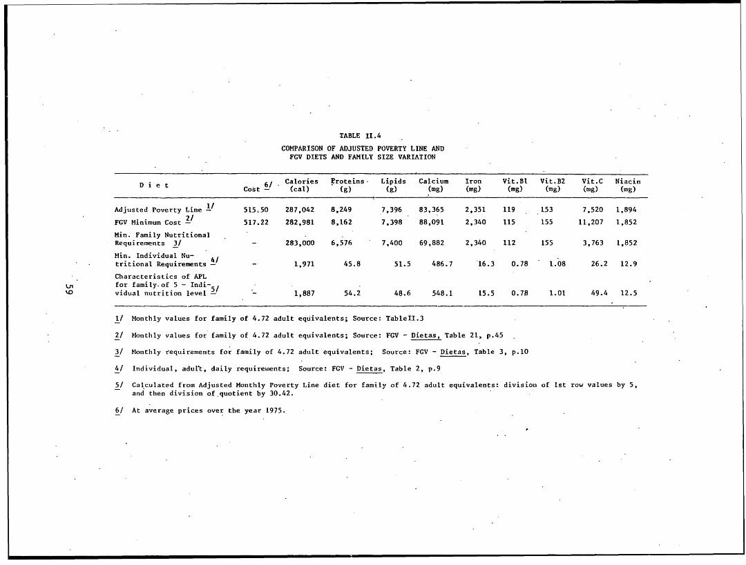
TABLE 11.4
COMPARISON OF ADJUSTED POVERTY LINE ANDFGV DIETS AND FAMILY SIZE VARIATION
D i e t 6/ Calories Proteins- Lipids Calcium Iron Vit.B1 Vit.B2 Vit.C NiacinCost - (cal) (g) (g) (mg) (mg) (mg) (mg) (mg) (mg)
Adjusted Poverty Line 515.50 287,042 8.249 7,396 83,365 2,351 119 153 7,520 1,894FGV Minimum Cost -3 517.22 282,981 8,162 7,398 88,091 2,340 115 155 11,207 1,852Hin. Family NutritionalRequirements 3/ - 283,000 6,576 7,400 69,882 2,340 112 155 3,763 1,852Min. Individual Nu-tritional Requirements - - 1,971 45.8 51.5 486.7 16.3 0.78 1.08 26.2 12.9Characteristics of APL
Ln for family-of 5 - Indi-'. vidual nutrition level - - 1,887 54.2 48.6 548.1 15.5 0.78 1.01 49.4 12.5
1/ Monthly values for family of 4.72 adult equivalents; Source: TableII.3
2/ Monthly values for family of 4.72 adult equivalents; Source: FGV - Dietas, Table 21, p.45
3/ Monthly requirements for family of 4.72 adult equivalents; Source: FGV - Dietas, Table 3, p.10
4/ Individual, adurt, daily requirements; Source: FGV - Dietas, Table 2, p.9
5/ Calculated from Adjusted Monthly Poverty Line diet for family of 4.72 adult equivalents: division of 1st row values by 5,and then division of quotient by 30.42.
6/ At average prices over the year 1975.-
ANNEX III
TABLES III.1 - I.15 PRESENTING
SIZE DISTRIBUTION OF FAMILY EXPENDITURES
BY ENDEF REGIONS
60
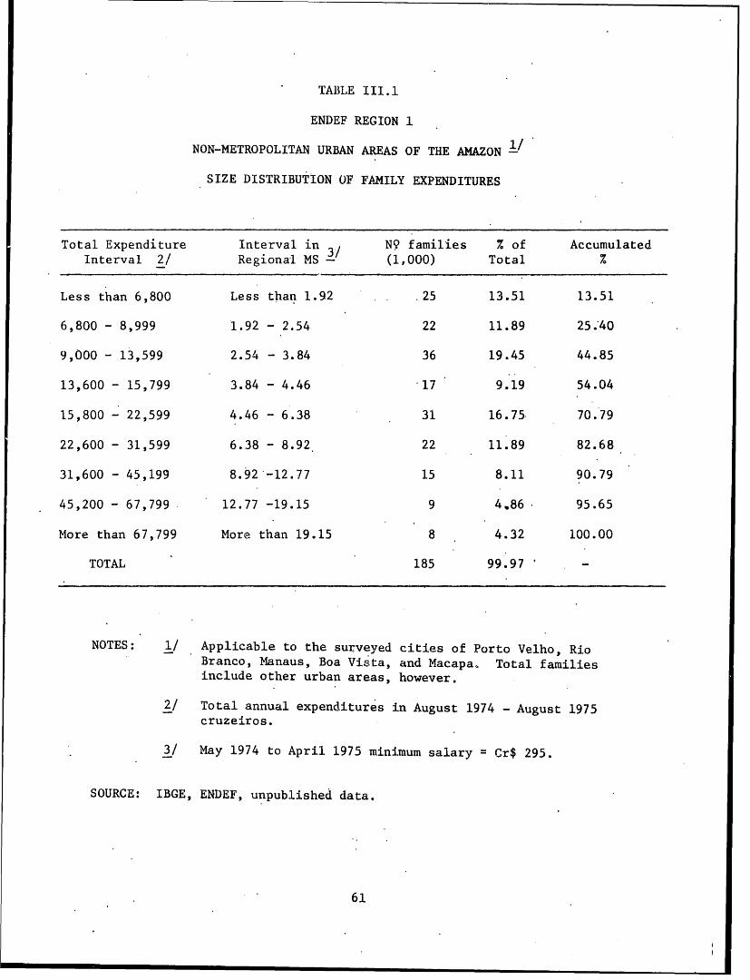
TABILE III.1
ENDEF REGION 1
NON-METROPOLITAN URBAN AREAS OF THE AMAZON
SIZE DISTRIBUTION OF FAMILY EXPENDITURES
Total Expenditure Interval in NO families % of AccumulatedInterval 2/ Regional MS 3 (1,000) Total %
Less than 6,800 Less than 1.92 25 13.51 13.51
6,800 - 8,999 1.92 - 2.54 22 11.89 25.40
9,000 - 13,599 2.54 - 3.84 36 19.45 44.85
13,600 - 15,799 3.84 - 4.46 17 9.19 54.04
15,800 - 22,599 4.46 - 6.38 31 16.75 70.79
22,600 - 31,599 6.38 - 8.92, 22 11.89 82.68
31,600 - 45,199 8.92-12.77 15 8.11 90.79
45,200 - 67,799 12.77 -19.15 9 4.86 95.65
More than 67,799 More than 19.15 8 4.32 100.00
TOTAL 185 99.97
NOTES: 1/ Applicable to the surveyed cities of Porto Velho, RioBranco, Manaus, Boa Vista, and Macapa, Total familiesinclude other urban areas, however.
2/ Total annual expenditures in August 1974 - August 1975cruzeiros.
3/ May 1974 to April 1975 minimum salary = Cr$ 295.
SOURCE: IBGE, ENDEF, unpublished data.
61
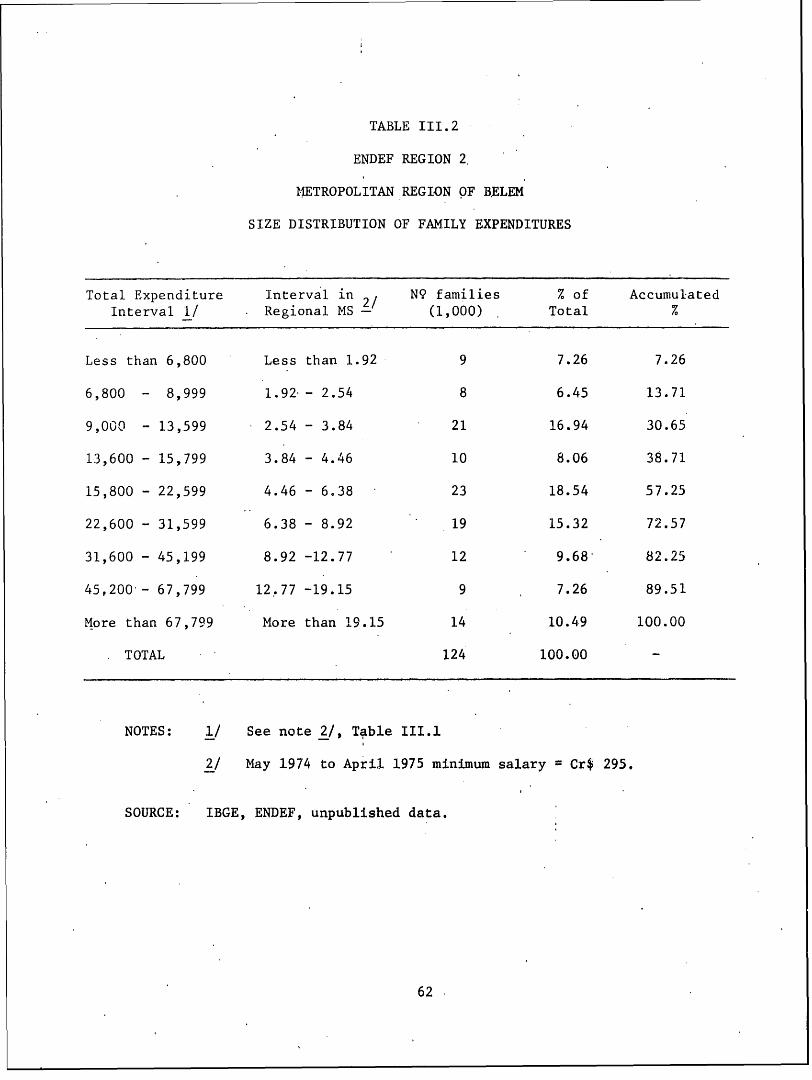
TABLE III.2
ENDEF REGION 2.
METROPOLITAN REGION OF BELEM
SIZE DISTRIBUTION OF FAMILY EXPENDITURES
Total Expenditure I'nterval in 2/ N9 families % of AccumulatedInterval 1/ Regional MS - (1,000) Total %
Less than 6,800 Less than 1.92 9 7.26 7.26
6,800 - 8,999 1.92 - 2.54 8 6.45 13.71
9,000 - 13,599 2.54 - 3.84 21 16.94 30.65
13,600 - 15,799 3.84 - 4.46 10 8.06 38.71
15,800 - 22,599 4.46 - 6.38 23 18.54 57.25
22,600 - 31,599 6.38 - 8.92 19 15.32 72.57
31,600 - 45,199 8.92 -12.77 12 9.68 82.25
45,200 - 67,799 12 .77 -19.15 9 7.26 89.51
More than 67,799 More than 19.15 14 10.49 100.00
TOTAL 124 100.00
NOTES: 1/ See note 2/, Table III.1
2/ May 1974 to April 1975 minimum salary = Cr$ 295.
SOURCE: IBGE, ENDEF, unpublished data.
62
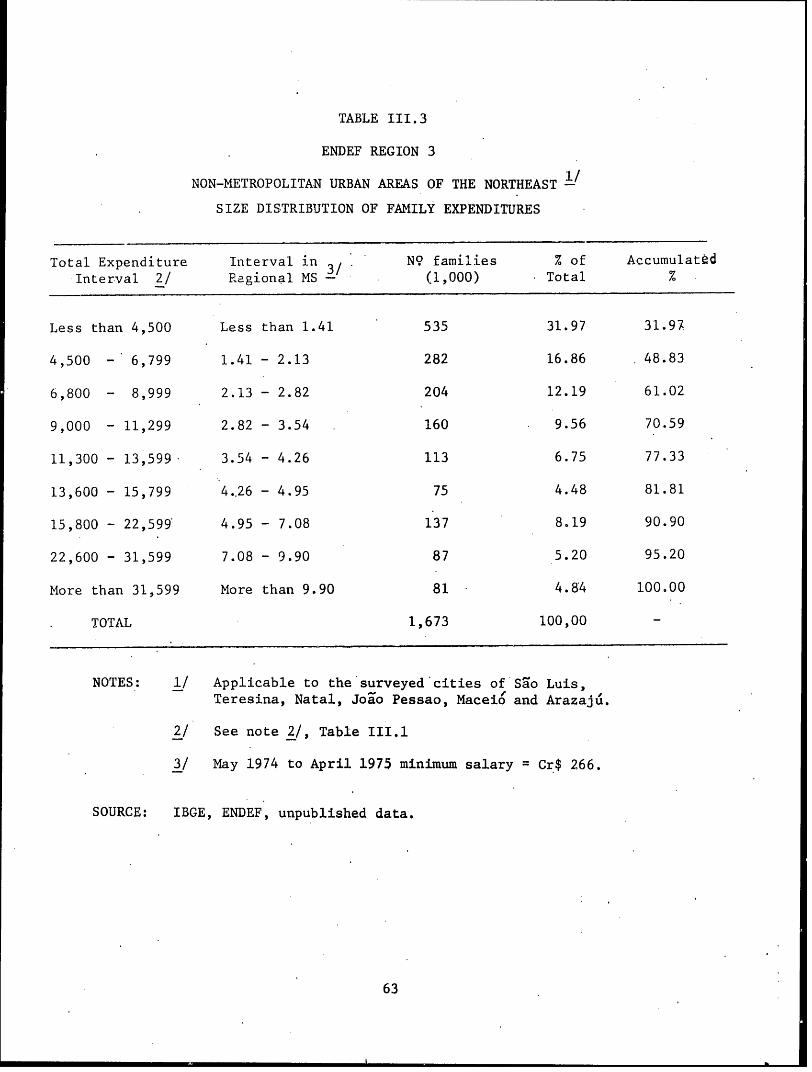
TABLE III.3
ENDEF REGION 3
NON-METROPOLITAN URBAN AREAS OF THE NORTHEAST -
SIZE DISTRIBUTION OF FAMILY EXPENDITURES
Total Expenditure Interval in 3/ N° families % of AccumuatInterval 2/ Regional MS - (1,000) Total
Less than 4,500 Less than 1.41 535 31.97 31.97
4,500 - 6,799 1.41 - 2.13 282 16.86 48.83
6,800 - 8,999 2.13 - 2.82 204 12.19 61.02
9,000 - 11,299 2.82 - 3.54 160 9.56 70.59
11,300 - 13,599 3.54 - 4.26 113 6.75 77.33
13,600 - 15,799 4..26 - 4.95 75 4.48 81.81
15,800 - 22,599 4.95 - 7.08 137 8.19 90.90
22,600 - 31,599 7.08 - 9.90 87 5.20 95.20
More than 31,599 More than 9.90 81 4.84 100.00
TOTAL 1,673 100,00 -
NOTES: 1/ Applicable to the surveyed cities of Sao Luis,Teresina, Natal, Joao Pessao, Maceio' and Arazajui.
2/ See note 2/, Table III.1
3/ May 1974 to April 1975 minimum salary = Cr$ 266.
SOURCE: IBGE, ENDEF, unpublished data.
63
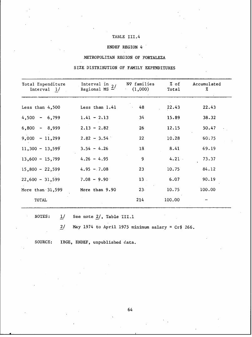
TABLE III.4
ENDEF REGION 4*
METROPOLITAN REGION OF FORTALEZA
SIZE DISTRIBUTION OF FAMILY EXPENDITURES
Total Expenditure Interval in 2/ N° families % of AccumulatedInterval 1/ Regional MS (1,000) Total %
Less than 4,500 Less than 1.41 48 22.43 22.43
4,500 - 6,799 1.41 - 2.13 34 15.89 38.32
6,800 - 8,999 2.13 - 2.82 26 12.15 50.47
9,000 - 11,299 2.82 - 3.54 22 10.28 60.75
11,300 - 13,599 3.5.4 - 4.26 18 8.41 69.19
13,600 - 15,799 4.26 - 4.95 9 4.21 73.37
15,800 - 22,599 4.95 - 7.08 23 10.75 84.12
22,600 - 31,599 7.08 - 9.90 13 6.07 90.19
More than 31,599 More than 9.90 23. 10.75 100.00
TOTAL 214 100.00
NOTES: 1/ See note 2/, Table III.1
2/ May 1974 to April 1975 minimum salary Cr$ 266.
SOURCE: IBGE, ENDEF, unpublished data.
64
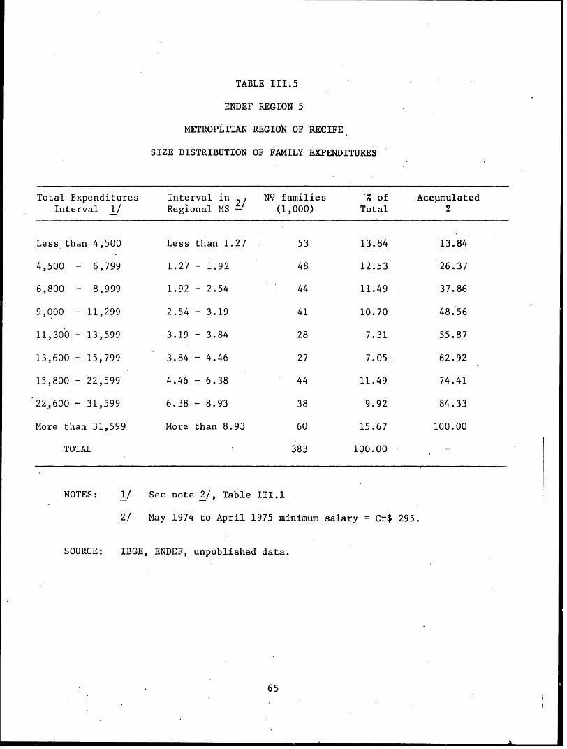
TABLE III.5
ENDEF REGION 5
METROPLITAN REGION OF RECIFE
SIZE DISTRIBUTION OF FAMILY EXPENDITURES
Total Expenditures Interval in N9 families I of AccumulatedInterval 1/ Regional MS (1,000) Total Z
Less than 4,500 Less than 1.27 53 13.84 13.84
4,500 - 6,799 1.27 - 1.92 48 12.53 26.37
6,800 - 8,999 1.92 - 2.54 44 11.49 37.86
9,000 - 11,299 2.54 - 3.19 41 10.70 48.56
11,300 - 13,599 3.19 - 3.84 28 7.31 55.87
13,600 - 15,799 3.84 - 4.46 27 7.05 62.92
15,800 - 22,599 4.46 - 6.38 44 11.49 74.41
22,600 - 31,599 6.38 - 8.93 38 9.92 84.33
More than 31,599 More than 8.93 60 15.67 100.00
TOTAL 383 100.00
NOTES: 1/ See note 2/, Table III.1
2/ May 1974 to April 1975 minimum salary = Cr$ 295.
SOURCE: IBGE, ENDEF, unpublished data.
65
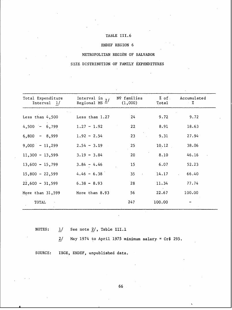
TABLE III.6
ENDEF REGION 6
METROPOLITAN REGION OF SALVADOR
SIZE DISTRIBUTION OF FAMILY EXPENDITURES
Total Expenditure Interval in N9 families % of, AccumulatedInterval 1/ Regional MS (1,000) Total %
Less than 4,500 Less than 1.27 24 9.72 9.72
4,500 - 6,799 1.27 - 1.92 22 8.91 18.63
6,800 - 8,999 1.92 - 2.54 23 9.31 27.94
9,000 - 11,299 2.54 - 3.19 25 10.12 38.06
11,300 - 13,599. 3.19 - 3.84 20 8.10 46.16
13,600 - 15,799 3.84 - 4.46 15 6.07 52.23
15,800 - 22,599 4.46 - 6.38 35 14.17 66.40
22,600 - 31,599 6.38 - 8.93 28 11.34 77.74
More than 31,599 More than 8.93 56 22.67 100.00
TOTAL 247 100.00
NOTES: 1/ See note 2/, Table III.1
2/ May 1974 to April 1975 minimum salary = Cr$ 295.
SOURCE: IBGE, ENDEF, unpublished data.
66
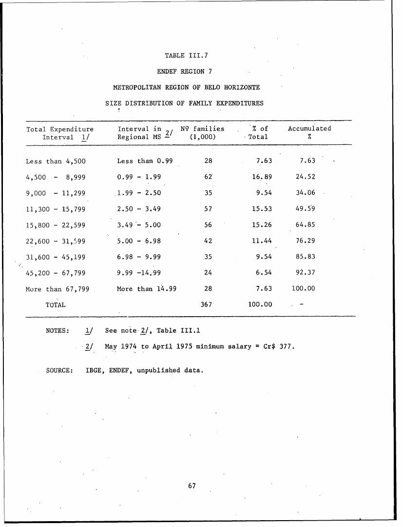
TABLE III.7
ENDEF REGION 7
METROPOLITAN REGION OF BELO HORIZONTE
SIZE DISTRIBUTION OF FAMILY EXPENDITURES
Total Expenditure Interval in N9 families . % of AccumulatedInterval 1/ Regional MS (1,000.) Total %
Less than 4,500 Less than 0.99 28 7.63 7.63
4,500 - 8,999 0.99 - 1.99 62 16.89 24.52
9,000 - 11,299 .1.99 - 2.50 35 9.54 34.06
11,300 - 15,799 2.50 - 3.49 57 15.53 49.59
15,800 - 22,599 3.49 - 5.00 56 15.26 64.85
22,600 - 31,599 5.00 - 6.98 42 11.44 76.29
31,600 - 45,199 6.98 - 9.99 35 9.54 85.83
45,200 - 67,799 9.99 -14.99 24 6.54 92.37
More than 67,799 More than 14.99 28 7.63 100.00
TOTAL 367 100.00
NOTES: 1/ See note 2/, Table III.1
2/ May 1974 to April 1975 minimum salary = Cr$ 377.
SOURCE: IBGE, ENDEF, unpublished data.
67
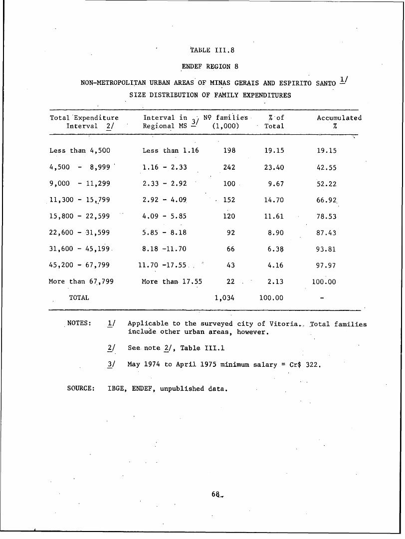
TABLE III.8
ENDEF REGION 8
NON-METROPOLITAN URBAN AREAS OF MINAS GERAIS AND ESPIRITO SANTO
SIZE DISTRIBUTION OF FAMILY EXPENDITURES
Total Expenditure Interval in - NQ families %-of Accumulated3/
Interval 2/ Regional MS - (1,0.00) Total %
Less than 4,500 Less than 1.16 198 19.15 19.15
4,500 - 8,999 1.16 - 2.33 242 23.40 42.55
9,000 - 11,299 2.33 - 2.92 100 9.67 52.22
11,300 - 15,7?99 2.92 - 4.09 152 14.70 66.92
15,800 - 22,599 4.09 - 5.85 120 11.61 78.53
22,600 - 31,599 5.85 - 8.18 92 8.90 87.43
31,600 - 45,199. 8.18 -11.70 66 6.38 93.81
45,200 - 67,799 11.70 -17.55. 43 4.16 97.97
More than 67,799 More than 17.55 22 2.13 100.00
TOTAL 17034 100.00 -
NOTES: 1/ Applicable to the surveyed city of Vitoria.. Total familiesinclude other urban areas, however.
2/ See note 2/, Table III.1
3/ May 1974 to April 1975 minimum salary Cr$ 322.
SOURCE: IBGE, ENDEF, unpublished data.
64-
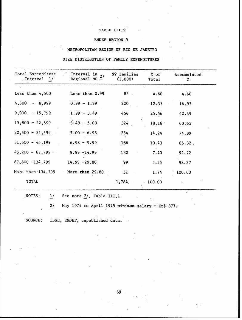
TABLE 111. 9
ENDEF REGION 9
METROPOLITAN REGION OF RIO DE JANEIRO
SIZE DISTRIBUTION OF FAMILY EXPENDITURES
Total Expenditure Interval in N9 families % of AccumulatedInterval 1/ Regional MS - (1,000) Total %
Less than 4,500 Less than 0.99 82 4.60 4.60
4,500 8,999 0.99 - 1.99 220 12.33 16.93
9,000 - 15,799 1.99 - 3.49 456 25.56 42,49
15,800 22,599 3.49 - 5.00 324 18.16 60.65
22,600 - 31,599, 5.00 - 6.98 254 14.24 74.89
31,600 - 45,199 6.98 - 9.99 186 10.43 85.32
45,200 - 67,799 9.99 -14.99 132 7.40 92.72
67,800 -134,799 14.99 -29.80 99 5.55 98.27
More than 134,799 More than 29.80 31 1.74 100.00
TOTAL 1,784. 100.00 -
NOTES: 1/ See note 2/, Table III.1
2/ May 1974 to April 1975 minimum salary = Cr$ 377.
SOURCE: IBGE, ENDEF, unpublished data.
69
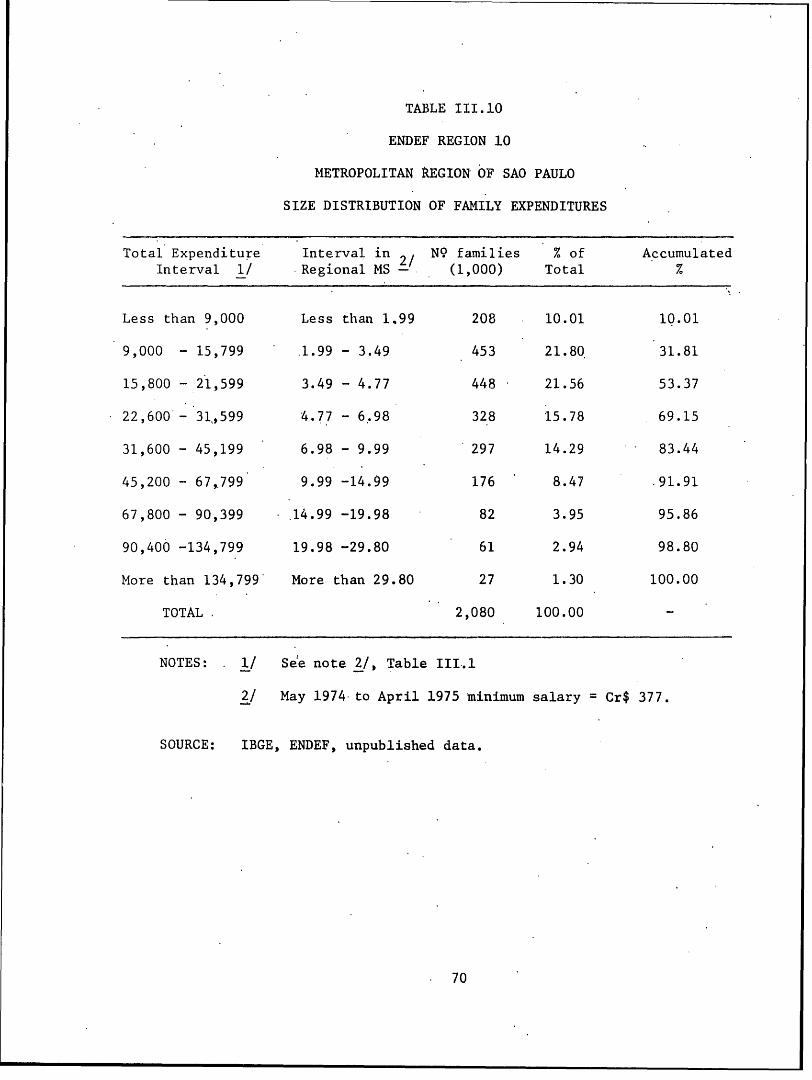
TABLE III.10
ENDEF REGION 10
METROPOLITAN REGION OF SAO PAULO
SIZE DISTRIBUTION OF FAMILY EXPENDITURES
Total Expenditure Interval in NQ families % of Accumulated2/
Interval 1/ Regional MS - (1,000) Total %
Less than 9,000 Less than 1.99 208 10.01 10.01
9,000 - 15,799 .1.99 - 3.49 453 21.80 31.81
15,800 - 21,599 3.49 - 4.77 448 21.56 53.37
22,600 - 31,599 4.77 - 6.98 328 15.78 69.15
31,600 - 45,199 6.98 - 9.99 297 14.29 83.44
45,200 - 67,799 9.99 -14.99 176 8.47 .91.91
67,800 - 90,399 14.99 -19.98 82 3.95 95.86
90,400 -134,799 19.98 -29.80 61 2.94 98.80
More than 134,799 More than 29.80 27 1.30 100.00
TOTAL 2,080 100.00
NOTES: 1/ See note 2/, Table III.1
/ May 1974 to April 1975 minimum salary = Cr$ 377.
SOURCE: IBGE, ENDEF, unpublished data.
70
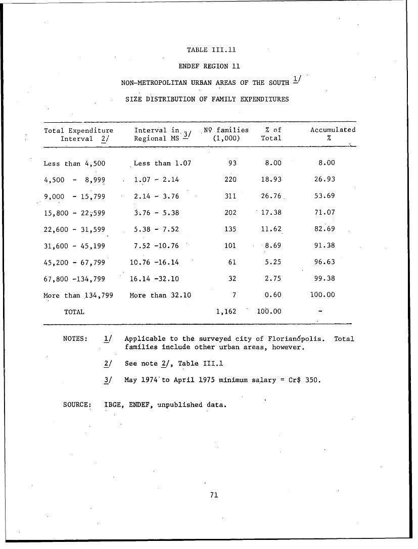
TABLE III.11
ENDEF REGION 11
NON-METROPOLITAN URBAN AREAS OF THE SOUTH
SIZE DISTRIBUTION OF FAMILY EXPENDITURES
Total Expenditure Interval in *N9 families % of AccumulatedInterval 2/ Regional MS - (1,000) Total %
Less than 4,500 Less than 1.07 93 8.00 8.00
4,500 - 8,999 . 1.07 - 2.14 220 18.93 26.93
9,000 - 15,799 2.14 - 3.76 311 26.76. 53.69
15,800 - 22;599 3.76 - 5.38 202 17.38 71.07
22,600 - 31,599 5.38 - 7.52 135 11.62 82.69
31,600 - 45,199 7.52 -10.76 101 *8.69 91.38
45,200 - 67,799 10.76 -16.14 61 5.25 96.63
67,800 -134,799 16.14 -32.10 32 2.75 99.38
More than 134,799 More than 32.10 7 0.60 100.00
TOTAL 1,162 100.00 -
NOTES: 1/ Applicable to the surveyed city of Florian6polis. Totalfamilies include other urban areas, however.
2/ See note 2/, Table III.1
3/ May 1974 to April 1975 minimum salary = Cr$ 350.
SOURCE: IBGE, ENDEF, unpublished data.
71
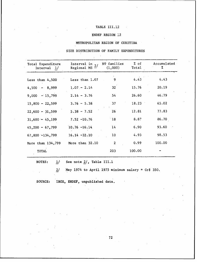
TABLE III.12
ENDEF REGION 12
METROPOLITAN REGION OF CURITIBA
SIZE DISTRIBUTION OF FAMILY EXPENDITURES
Total Expenditure Interval in NQ families % of AccumulatedInterval 1/ Regional MS - (1,000) Total %
Less than 4,500 Less than 1.07 9 4.43 4.43
4, 500 8,999 1.07.- 2.14 32 15.76 20.19
9,000 - 15,799 2.14 - 3.76 54 26.60 46.79
15,800 - 22,599 3.76 - 5.38 37 18.23 65.02
22,600 31,599 5.38 - 7.52 26 12.81 77.83
31,600- 45,199 7.52 -10.76 18 8.87 86.70
45,200 - 67,799 10.76 -16.14 14 6.90 93.60
67,800 -134,799 1.6.14 -32.10 10 4.93 98.53
More than 134,799 More than 32.10 2 0.99 100.00
TOTAL 203 100.00 -
NOTES: 1/ See note 2/, Table III.1
2/ May 1974 to April 1975 minimum salary = Cr$ 350.
SOURCE: IBGE, ENDEF, unpublished data.
72
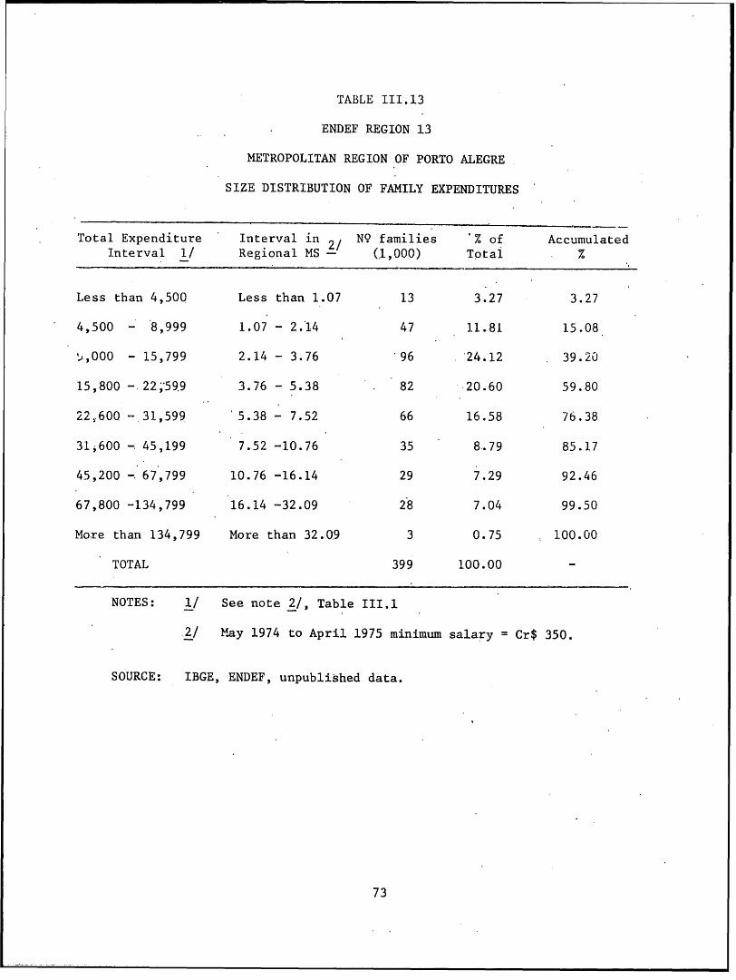
TABLE III.13
ENDEF REGION 13
METROPOLITAN REGION OF PORTO ALEGRE
SIZE DISTRIBUTION OF FAMILY EXPENDITURES
Total Expenditure Interval in NO families % of Accumulated
Interval 1/ Regional MS - (.1,000) Total %
Less than 4,500 Less than 1.07 13 3.27 3.27
4,500 - 8,999 1.07 - 2.14 47 11.81 15.08
'., 000 - 15,799 2.14 - 3.76 96 24.12 39.20
15,800 -. 22;,599 3.76 - 5.38 82 20.60 59.80
22,600 -. 31,599 5.38 - 7.52 66 16.58 76.38
31,600 - 45,199 7.52 -10.76 35 8.79 85.17
45,200 - 67,799 10.76 -16.14 29 7.29 92.46
67,800 -1343,799 16.14 -32.09 28 7.04 99.50
Mo.re than 134,799 More than 32.09 3 0.75 100.00
TOTAL 399 100.00 -
NOTES: 1/ See note 2/, Table III.1
2/ May 1974 to April 1975 minimum salary = Cr$ 350.
SOURCE: IBGE, ENDEF, unpublished data.
73
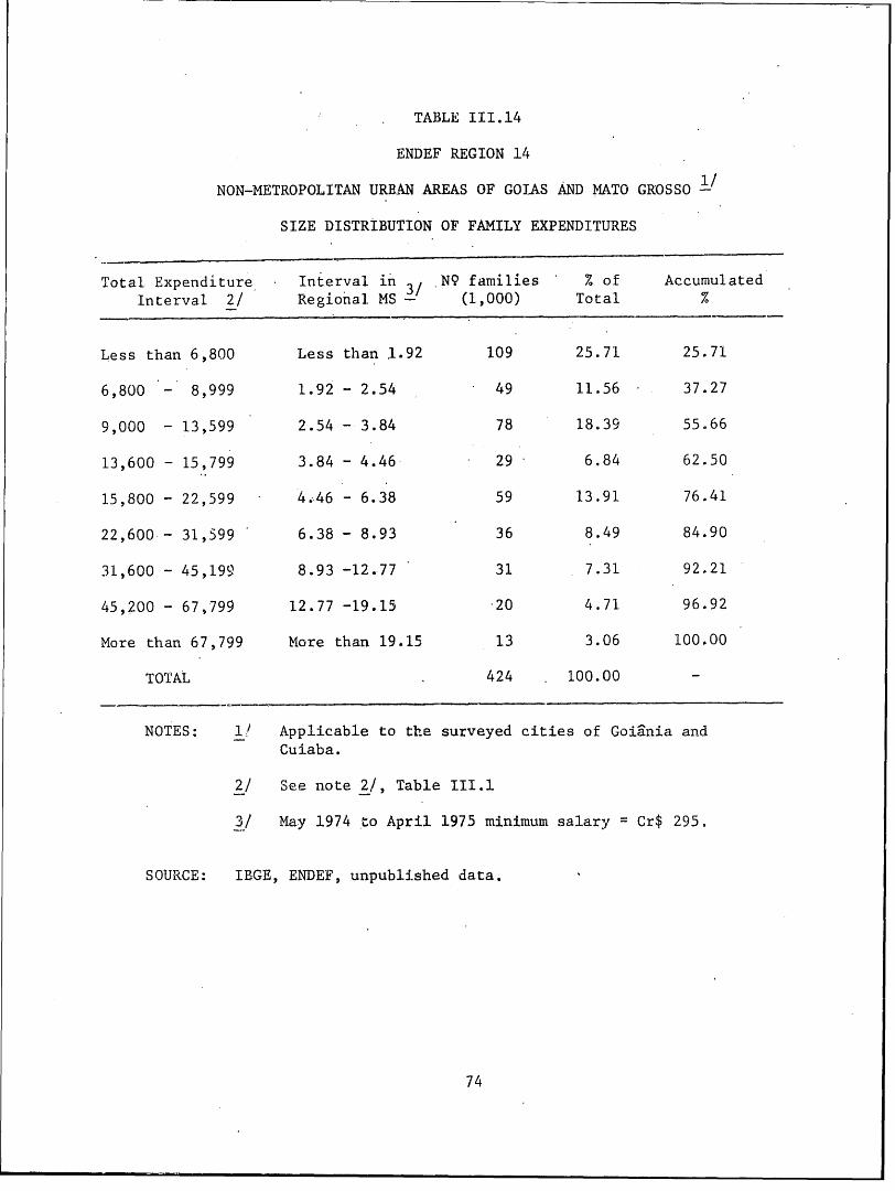
TABLE III.14
ENDEF REGION 14
NON-METROPOLITAN URBAN AREAS OF GOIAS AND MATO GROSSO 1,
SIZE DISTRIBUTION OF FAMILY EXPENDITURES
Total Expenditure Interval in 3/ NO families % of Accumulated
Interval 2/ Regional MS - (1,000) Total %
Less than 6,800 Less than 1.92 109 25.71 25.71
6,800 - 8,999 1.92 - 2.54 49 11.56 37.27
9,000 - 13,599 2.54 - 3.84 78 18.39 55.66
13,600 - 15,799 3.84 - 4.46 29 6.84 62.50
15,800 - 22,599 4.46 - 6.38 59 13.91 76.41
22,600 - 31,599 6.38 - 8.93 36 8.49 84.90
31,600 - 45,199 8.93 -12.77 31 7.31 92.21
45,200 - 67,799 12.77 -19.15 20 4.71 96.92
More than 67,799 More than 19.15 13 3.06 100.00
TOTAL . 424 100.00 -
NOTES: 1! Applicable to the surveyed cities of Goiania and
Cuiaba.
2/ See note 2/, Table III.1
3/ May 1974 to April 1975 minimum salary Cr$ 295.
SOURCE: IEGE, ENDEF, unpublished data.
74
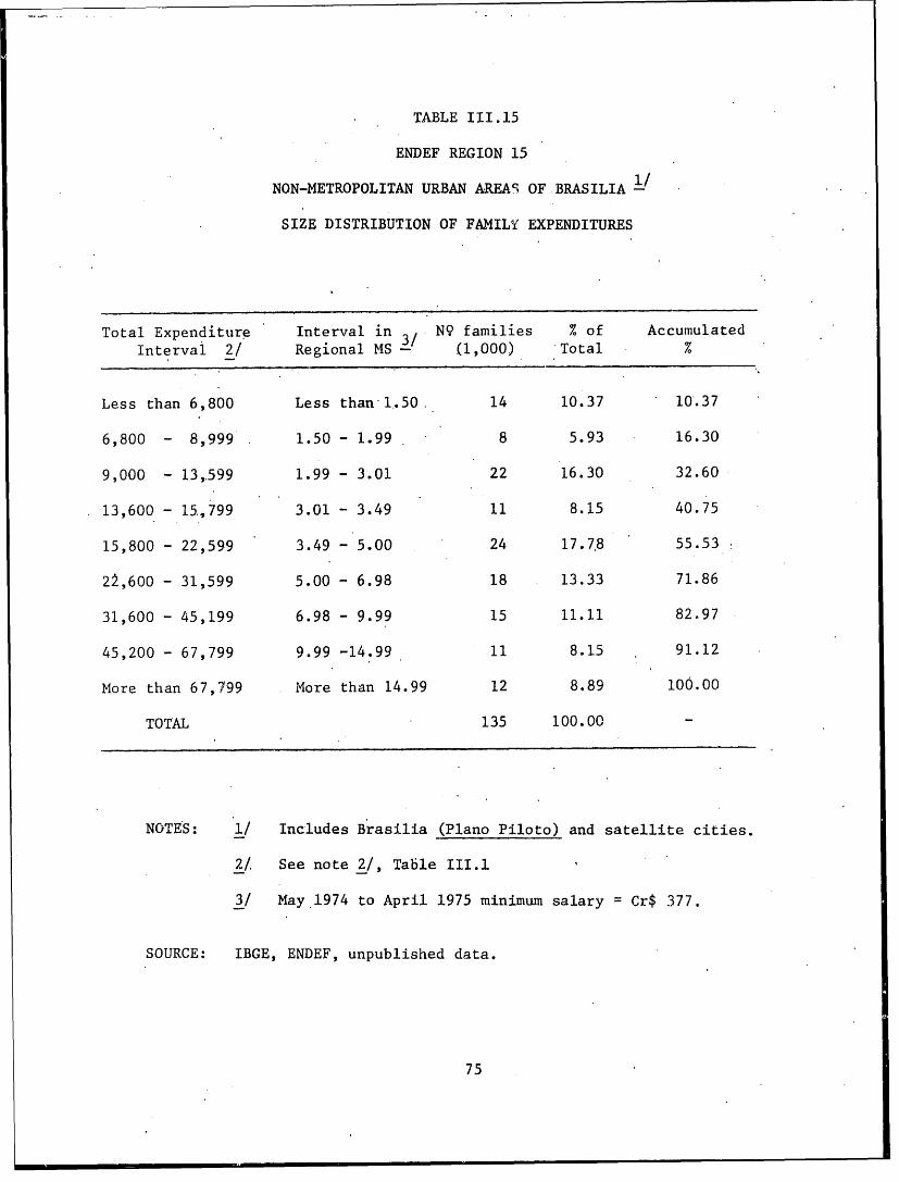
TABLE III.15
ENDEF REGION 15
NON-METROPOLITAN URBAN AREAS OF BRASILIA
SIZE DISTRIBUTION OF FAMILY EXPENDITURES
Total Expenditure Interval in N9 families % of AccumulatedIntervai 2/ Regional MS - (1,000) Total %
Less than 6,800 Less than 1.50. 14 10.37 10.37
6,800 - 8,999 1.50 - 1.99 8 5.93 16.30
9,000 - 13,599 1.99 - 3.01 22 16.30 32.60
13,600 - 15,799 3.01 - 3.49 11 8.15 40.75
15,800 - 22,599 3.49 - 5.00 24 17.78 55.53
22,600 - 31,599 5.00 - 6.98 18 13.33 71.86
31,600 - 45,199 6.98 - 9.99 15 11.11 82.97
45,200 - 67,799 9.99 -14.99 11 8.15 91.12
More than 67,799 More than 14.99 12 8.89 100.00
TOTAL 135 100.00 -
NOTES: 1/ Includes Brasilia (Plano Piloto) and satellite cities.
2/ See note 2/, Table III.1
3/ May 1974 to April 1975 minimum salary Cr$ 377.
SOURCE: IBGE, ENDEF, unpublished data.
75
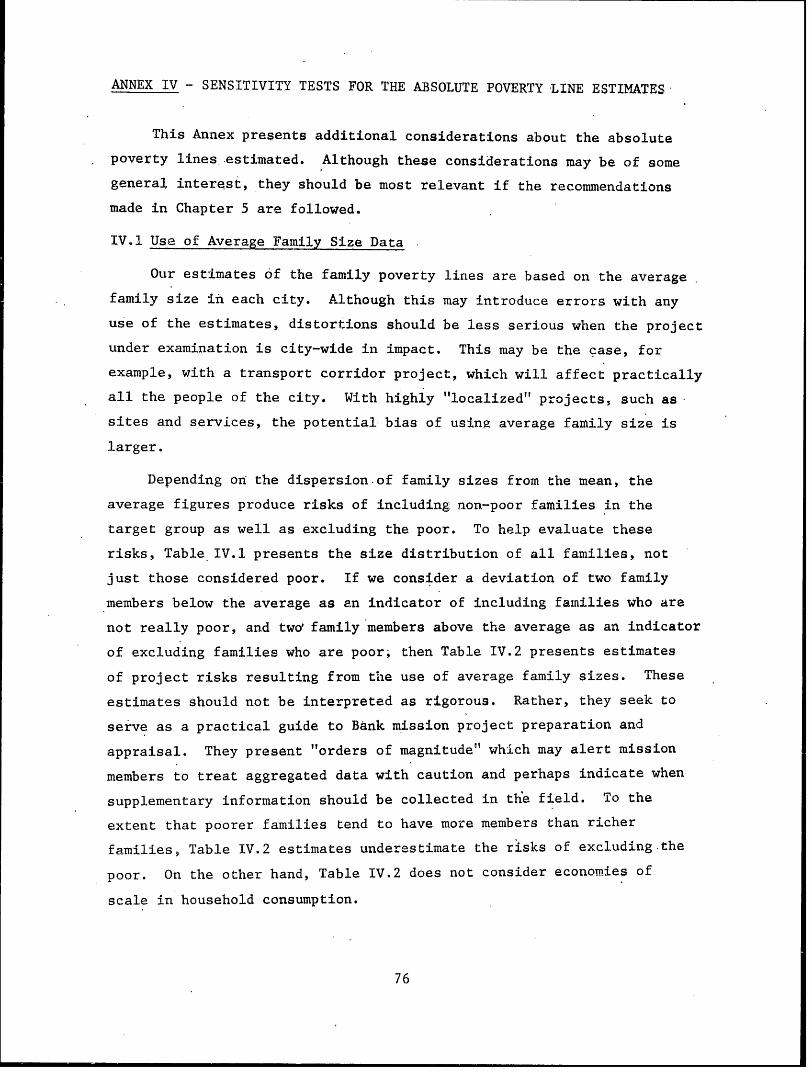
ANNEX IV - SENSITIVITY TESTS FOR THE ABSOLUTE POVERTY LINE ESTIMATES
This Annex presents additional considerations about the absolute
poverty lines estimated. Although these considerations may be of some
general interest, they should be most relevant if the recommendations
made in Chapter 5 are followed.
IV.1 Use of Average Family Size Data
Our estimates of the family poverty lines are based on the average
family size in each city. Although this may introduce errors with any
use of the estimates, distortions should be less serious when the project
under examination is city-wide in impact. This may be the case, for
example, with a transport corridor project, which will affect practically
all the people of the city. With highly "localized" projects, such as
sites and services, the potential bias of using average family size is
larger.
Depending on the dispersion-of family sizes from the mean, the
average figures produce risks of including non-poor families in the
target group as well as excluding the poor. To help evaluate these
risks, Table IV.1 presents the size distribution of all families, not
just those considered poor. If we consider a deviation of two family
members below the average as an indicator of including families who are
not really poor, and twd family members above the average as an indicator
of excluding families who are poor; then Table IV.2 presents estimates
of project risks resulting from thle use of average family sizes. These
estimates should not be interpreted as rigorous. Rather, they seek to
serve as a practical guide to Bank mission project preparation and
appraisal. They present "orders of magnitude" which may alert mission
members to treat aggregated data with caution and perhaps indicate when
supplementary information should be collected in tl•e field. To the
extent that poorer families tend to have more members than richer
families, Table IV.2 estimates underestimate the risks of excluding-the
poor. On the other hand, Table IV.2 does not consider economies of
scale in household consumption.
76
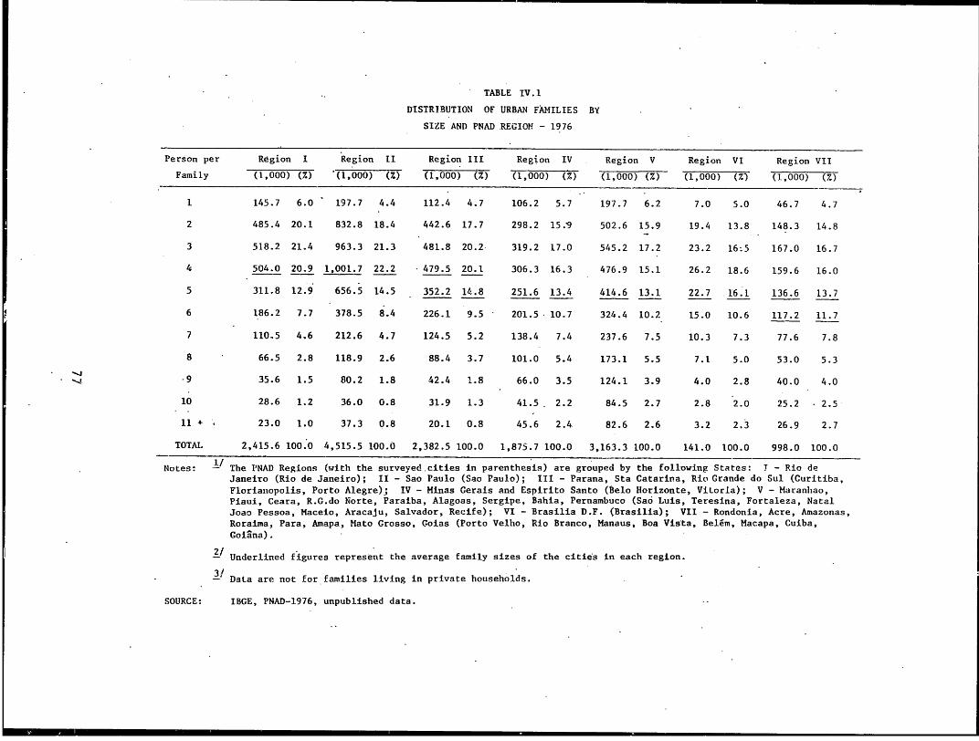
TABLE IV.1
DISTRIBUTION OF URBAN FAMILIES BY
SIZE AND PNAD .REGION - 1976
Person per Region I Region II Region III Region IV Region V Region VI Region VII
Family (1,000) (%) (1,000) (Z) (1,000) (%) (1,000) (%) (1,000) (%) (1,000) (%) (1,000) (%)
1 145.7 6.0 197.7 4.4 112.4 4.7 106.2 5.7 197.7 6.2 7.0 5.0 46.7 4.7
2 485.4 20.1 832.8 18.4 442.6 17.7 298.2 15.9 502.6 15.9 19.4 13.8 148.3 14.8
3 518.2 21.4 963.3 21.3 481.8 20.2 319.2 17.0 545.2 17.2 23.2 16 5 167.0 16.7
4 504.0 20.9 1,001.7 22.2 479.5 20.1 306.3 16.3 476.9 15.1 26.2 18.6 159.6 16.0
5 311.8 12.9 656.5 14.5 352.2 14.8 251.6 13.4 414.6 13.1 22.7 16.1 136.6 13.7
6 186.2 7.7 378.5 8.4 226.1 9.5 201.5- 10.7 324.4 10.2 15.0 10.6 117.2 11.7
7 110.5 4.6 212.6 4.7 124.5 5.2 138.4 7.4 237.6 7.5 10.3 7.3 77.6 7.8
8 66.5 2.8 118.9 2.6 88.4 3.7 101.0 5r4 173.1 5.5 7.1 5.0 53.0 5.3
-9 35.6 1.5 80.2 1.8 42.4 1.8 66.0 3.5 124.1 3.9 4.0 2.8 40.0 4.0
10 28.6 1.2 36.0 0.8 31.9 1.3 41.5 2.2 84.5 2.7 2.8 2.0 25.2 * 2.5
11 + 23.0 1.0 37.3 0.8 20.1 0.8 45.6 2.4. 82.6 2.6 3.2 2.3 26.9 2.7
TOTAL 2,415.6 100:0 4,515.5 100.0 2,382.5 100.0 1,875.7 100.0 3,163.3 100.0 141.0 100.0 998.0 100.0
Notes: - The PNAD Regions (with the surveyed.cities in parenthesis) are grouped by the following States: j - Rio deJaneiro (Rio de Janeiro); II - Sao Paulo (Sao Paulo); III - Parana, Sta Catarina, Rio Grande do Sul (Curitiba,Florianopolis, Porto Alegre); IV - Minas Gerais and Espirito Santo (Belo Horizonte, ViLorla); V - Maranliao,Piaui, Ceara, R.G.do Norte, Paralba, Alagoas, Sergipe, Bahia, Pernambuco (Sao Luis, Teresina, Fortaleza, NatalJoao Pessoa, Maceio, Aracaju, Salvador, Recife); VI - Brasilia D.F. (Brasilia); VII - Rondonia, Acre, Amazonas,Roraima, Para, Amapa., Mato Grosso, C.oias (Porto Velho, Rio Branco, Manaus, Boa Vista, Bel6m, Macapa, Cuiba,Goiana).
2/ Underlined figures represent the average family sizes of the cities in each region.
- DaLa are not for families living in private households.
SOURCE: IBGE, PNAD-1976, unpublished data.
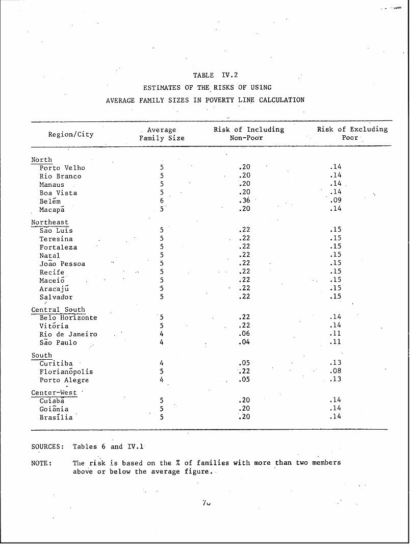
TABLE IV.2
ESTIMATES OF THE RISKS OF USING
AVERAGE FAMILY SIZES IN POVERTY LINE CALCULATION
Region/City Average Risk of Including Risk of ExcludingFamily Size Non-Poo:r Poor
NorthPorto Velho 5 .20 .14
Rio Branco 5 .20 .14
Manaus -5 20 .14
Boa Vista 5 .20 .14
Belem 6 .36 .09
Macapa 5 .20 .14
NortheastSao Luis 5 .22 .15
Teresina 5 - .22 .15
Fortaleza 5 .22 .15Natal 5 .22 .15Joao Pessoa 5 .22 .15Recife 5 . .22 .15
Maceio 5 .22 . .15Aracajiu 5 .22 .15Salvador 5 .22 .15
Central SouthBelo Horizonte 5 .22 .14Vitoria 5 . .22 .14Rio de Janeiro . 4 .06 .11Sao Paulo 4 .04 .11
SouthCuritiba 4 .05 .13Florianopolis 5 .22 .08Porto Alegre 4 .05 .13
Center-WestCuiaba 5 .20 .14Goiania 5 .20 .14Brasrlia 5 .20 .14
SOURCES: Tables 6 and IV.1
NOTE: The risk is based on the % of families with more than two membersabove or below the average figure.
IV.2 Use of Monetary Versus Non-Monetary Income Data
Sometimes data in Brazil do not include non-monetary income.
Assuming that in urban areas non-monetary income is basically derived
from imputed housing rents, ENDEF provides data which allow an estimate
of the impact of excluding these rents.
Previous poverty line estimates were based on the food share (s) of
total family budgets going to food. Excludin,g imputed rents from total
family expenditures decreases the denominator while the numerator remains
fixed. The new food share, xs, will, of course, be larger. This., in
turn, means that the poverty lines estimated with xs will be lower than
those estimated with s.
Table IV.3 presents new absolute poverty estimates based on xs.
Comparison of this Table's estimates with those presented in Tables 6
and 7 permits quick conversions from income data which do not include
non-monetary income to more complete income estimates.
IV.3 Use of Beahvioral Diet in Absolute Poverty Line Estimates
As discussed in Chapter 3 and Annex II, our definition of the
family minimum diet may have introduced a conservative bias in our
estimates. Actual expenditures of the FGV surveyed families vere almost
20% greater than the cost of the diet used here. Comparative price
shopping and other "information costs," as well as eating habits, may
cause the actual diet cost of low-income families to be substantially
greater than the cost estimated here. In addition, we adjusted the FGV
family size up, from 4.72 adult equivalents to 5 "imouths to feed."
This, of course, slightly reduces the per capita family food expenditures
estimates.
In order to off-set this potential bias, Table IV.4 presents 1980
poverty line estimates resulting from increasing the family mainimum diet
cost by 20%. Although these new estimates do not have direct relevance
to the present study, they may be useful in comparison with studies in
other countries or with future up-dates and extensions in Brazil, particularly
if new minimum cost, nutritionally adequate food baskets are defined
with more recent data.
79
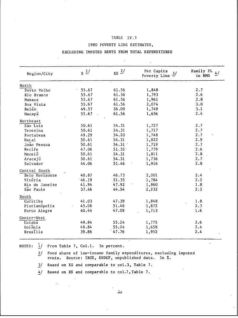
TABLE lV.3
1980 POVERTY LINE ESTIMATES,
EXCLUDING IMPUTED RENTS FROM TOTAL EXPENDITURES
l/ XS1 2/ Per Capita Family PLRegion/City - 3/ erCait
Poverty Line - in RMS -
NorthPorto Velho 55.67 61.56 1,848 2.7Rio Branco 55.67 61.56 1,793 2.6Manaus 55.67 61.56 1,961 2.8Boa Vista 55.67 61.56 2,074 3.0Belem 49.57 56.09 1,749 3.1Macapa 55.67 61.56 1,656 2.4
NortheastSao Luis 50.61 54.31 1,727 2.7Teresina 50.61 54.31 1,717 2.7Fortaleza 49.29 54.20 1,748 2.7NaLal 50.61 54.31 1,822 2.9Joao Pessoa 50.61 54.31 1,719 2.7Recife 47.06 51.35 1,779 2.6Maceio 50.61 54.31 1,811 2.8Aracajiu 50.61 54.31 1,736 2.7Salvador 44.06 51.46 - 1,916 2.8
Central SouthBelo Horizonte 40.87 46.73 2,001 2.4Vitoria 46.19 51.35 1,784 2.2Rio de Janeiro 41.94 47.92 1,860 1.8Sao Paulo 37.46 44.54 2,232 2.2
SouthCuritiba 41.03 47.39 1,848 1.8Florianopolis 45.06 51.46 1,872 2.3Porto Alegre 40.44 47.09 1,713 1.6
Center-WestCuiaba 49.84 55.24 1,775 2.6Goiainia 49.84 55.24 1,658 2.4Brasrlia 39.86 47.76 1,952 2.4
NOTES: 1/ -From Table 7, Col.l. In percent.
2/ Food share of low-income family expenditures, excluding imputedrents. Source: IBGE, ENDEF, unpublished data. In %.
3/ Based on XS and comparable to col.3, Table 7.
4/ Based on XS and comparable to col.7,Table 7.
o3u
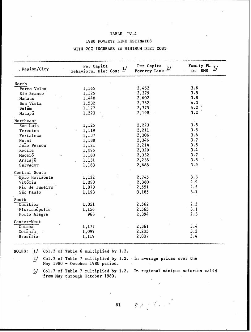
TABLE IV.4
1980 POVERTY LINE ESTIMATES
WITH 20% INCREASE i-vi MINIMUM DIET COST
Per Capita 1 Per Capita 2 Family PL'Behavioral Diet Cost - Poverty Line - in RMS -
NorthPorto Velho 1,365 2,452 3.6Rio Branco 1,325 2,379 3.5Manaus 1,448 2,602 3.8Boa Vista 1,532 2,752 4.0Belem 1,177 2,375 4.2Macapa 1,223 2,198 3.2
NortheastSao Luis 1,125 2,223 3.5Teresina 1,119 2,211 3.5Fortaleza 1,137 2,306 3.6Natal 1,188 2,346 3.7Joao Pessoa 1,121 2,214 3.5Recife 1,096 2,329 3.4Maceio 1,180 2,332 3.7Aracaju 1,131 2,235 3.5Salvador 1,183 2,685 3.9
Central SouthBelo Horizonte 1,122 2,745 3.3Vitoria 1,090 2,380 2.9Rio de Janeiro" 1,070 2,551 2.5Sao Paulo 1,193 3,185 3.1
SouthiCuritiba 1,051 2,562 2.5Florianopolis 1,156 2,565 3.1Porto Alegre 968 2,394 2.3
Center-WestCuiaba 1,177 2,361 3.4Goiania. 1,099 2,205 3.2Brasllia 1,119 2,807 3.4
NOTES: 1/ Col.2 of Table 6 multiplied by 1.2.
2/ Col.3 of Table 7 multiplied by 1.2. In average prices over theMay 1980 - October 1980 period.
3/ Col.7 of Table 7 multiplied by 1.2. In regional minimum salaries validfrom May through October 1980.
81 ,
World BankPublicationsof RelatedInterest
NEW
The Determinants of Labour income countries in terms of a num- Economic Growth andEarnings in Developing ber of socioeconomic indicators, it is Employment in ChinaMetropolises: Estimates noted that there are large regional Thomas G. Rawskidisparities between the northeast andfrom Bogota and Cal, the southeast with the northeast far- Examines how China's agriculturalColombia ing about the same as most low- sector has made significant stridesRakesh Mohan income countries. toward full employrnent for a laborforce of nearly half a billion persons.Examines the patterns of behavior World Bank Staff Working Paper No.
implicit in the variation of labor eam- 505. February 1982. 91 pages (includ- Oxford University Press, 1979.ings in Bogota and Call, Colombia. ing references, map). 208 pages (including maps, bibliogra-World Bank Staff Working Paper No. Stock No. WP-0505. $3.00. phy, index).498. October 1981.135 pages (Includ- LC 79-19550. ISBN 0-19-520151-5,ing 2 appendixes, bibliography). $18.95 hardcover. ISBN 0-19-520152-3,Stock No. WP-0498. $5.00. The Distribution of $7.95 paperback.
Income in Brazil French: Croissance et emploi en Chine.Guy e Pfeffermann and Economica, 1980.
NIEW Richard C. Webb ISBN 2-7178-0282-7,39 francs.
Differences In Income, World Bank Staff Working Paper No. Spanish: Crecimiento econ6mico yutrition, ad Poverty356. September 19 79. 116 pages empleo en China. Editorial Tecnos,wutithion, Bazil Pvry(Including 2 appendixes). 1980.within Brazil Stock No WP-0356. $5.00 180Vinod Thomas S N ISBN 84-309-0871-4, 600 pesetas.Regional disparities in living stan-dards in Brazil are examined and Employment Pattemsestimates for real income and nutri- amtional levels and poverty for maJor and Income Growthurban and rural areas are provided. Joseph J. Stern andAlthough the growth rate of the coun- Jeffrey D. Lewistry surpasses the average for most World Bank Staf Working Paper No,developing countries and the country 419 k Stembe rking Pagesperforms as well as many middle- 419. September 1980. 70 pages
(including bibliography, 2 appen-dixes).Stock No. WP-0419. $3.00.
Employment Policy in Household Income or Income Distrution PolicyDeveloping Countries: Household Income In the Developing CounA Survey of Issues per Capita in Welfare tries: A Case Study of Koreaand Evidence Comparisons Irma Adelman andLyn Squire C}autam Datta and Sherman RobinsonLow rates of growth in industrial Jacob Meerman Seeks to answer the question of howermployment, high rates of unemploy- World Bank Staff Working Paper No. much can actually be done toment among new entrants to the 378. March 1980. 32 pages (including improve income distribution byurban labor market, and low levels of 3 edlxr ee means of a dynamo c generallabor productivity and remuneration appenes, rerences. equilibrium model for investigatingare the three Issues addressed in this Stock No. WP-03 78. $3.00. the potential impact of standardstudy. The author identifles the impor- policy instruments and programstant determinants of labor demand intended to improve the relative andand supply and the extent to which How Segmented is the absolute incomes of the poor.the growth of labor demand has been Bogota Labor Market? Stanford Universityj Press, Stanford,constrained-and labor supply Gar S. Fields CalIforia 94305, U.S.A. (except theadvanced-by inaDpropriate policies.On the demand side, industrial trade World Bank Staff Working Paper No. United lKingdom and the Common-policy, agricultural growth, and the 434. October 1980. 99 pages (includ- wealth Market). 1978. Oxford Universityoperation of capital markets are ing bibliography). Press (except Mexico, United States,discussed; on the supply side, atten- SokN.1'644 30 and Canada). 1978. 364 pages (includ-tion is focused on population and Stock No. WP-0434. $3.00. ing 6 appendixes, index).education policy. LC 76-14269. ISBN 0-8047-0925-4
Oxford University Prss, 1981. 242 Incidence of Poverty and (Stanford), $12.50 hardcover.pages (Including bibliography, Index). the Characteristics of ISBN1 0-19-920084-X (Oxford), £7.50
LC 81-2844. ISBN 0-19-520266-X, the Poor in Peninsular hardcover.$16.95 (£11.50) hardcover; ISBN Malaysia, 19730-19-520267-8, $7.95 (£5.00) Pravin Visaria Income Inequality andpaperback. Examines the results of the Poverty: Methods of Estima-
Household Expenditure and Income tion and Policy ApplicationsGrowth and Equity In Semi- Survey conducted In peninsular Nand C. AniMalaysia during 1973 In order toNaaC.lkanIndustrialized Countries understand better the correlates Deals with income distribution
Joel Bergsman of poverty. methods and their economic
World Bank Staff Working Paper No. World Bank Staff Working Paper No. applications.351. August 1979. ii + 113 pages 460. May 1981. viii + 213 pages Oxford University Press, 1980. 432(including references). (including statistical appendix). pages (including bibliography,
Stock No. WP-0351. $5.00. Stock No. WP-0460. $10.00. Indexes).LC 80-14229. ISBN 0-19-520227-9,
Growth with Equity: Income Distribution $12.95 paperback.The Taiwan Case and Poverty in MexicoJohn C. H. Fei, Gustav Ranis, Joel Bergsman NEWand Shirley W. Y. Kuo World Bank Staff Working Paper No.
Introduces a method for tracing 395. July 1980. 46 pages (including Inequality and Povertythe inequality of family income to references). in Malaysia:the inequality of various kinds of Stock No. WP-0395. $3.00. Measurement andfactor Income and the shares 'e'p'toof factor income In family income. DeomPosIAtion
Siudhir AnandOxford University Press, 1980. An account of Income Inequalities444 pages (including index). and poverty in Malaysia. The research
LC 79-23354. ISBN 0-19-520115-9, Is policy oriented and the findings, to$27.50 (£10.25) hardcover; which the author's statistical tech-ISBN 0-19-520116-7, $12.95 nique is applied, are thoroughly(£4.25) paperback. discussed. A range of issues is
covered, from data problems to con- regarding links between human Studies the evolution of the structureceptual questions arising with respect development and labor productivity of consumer preferences as a func-to measurement. and focuses on policy measures tion of economic development.Oxford University Press. 1982, 384 aimed at raising the productivity of Oxford University Press, 1977. 312pages (including bibliography, index). dteveopment pages (including bibliography,LC 81-14178. ISBN 0-19-520153-1, World Bank Staff Working Paper No.)$27.50 hardcover. 497. October1981. ii + 70pages LC 77-3442. ISBN 0-19-920097-1,
(incudig bbliorapy).$22.50 hardcover;(including bibliography). ISBN 0-19-920100-5, $12.95Intemnational Migrant Stock No. WP-0497. $3.00. paperback.Workers' Remittances:
Isues and Prospects NEW Policy Interventions forGurushri Swamy Technological Innovation InA background study for World Manpower and Intemational Developing CountriesDevelopment Report 1981. Putstogether available data on intema- Labor Migration In the Mid- Charles Coopertional migrant workers' remittances to dle East and North Africa World Bank Staff Working Paper No.developing countries and analyzes Ismail Serageldin, James A. 441. December 1980. 59 pagesthe regional structure of and growth Socknat, Stace Birks, Bob Li, (including references).in these flows. Relates the flow of C , clairremittances to the level of and fluc- and Clive A. Sinclair Stock No. WP-0441. $3.00.tuations in economic activity and to This study of labdr market trends ininflation in the host countries and the region from 1975 to 1985attempts to forecast future demand analyzes the demand for and supply Poverty and Growthfor migrant labor and the likely of manpower by country, sector, in Kenyagrowth in remittances. occupation, sex, educational level, Paul Collier and Deepak Lal
Worl Bak Stff orkng PperNo. and ethnic composition. It indicatesWorld Bank Staff Working Paper No. the sources and destinations of World Bank Staff Working Paper No.481. August 1981. 64 pages (including workers and examines the social and 389. May 1980. 76 pages (including2 appendixes, bibliography). economic effects of migration for 2 appendixes, bibliography).Stock No. WP-0481. $3.00. both importers and exporters, par-
ticularly the implications for Stock No. WP-0389. $3.00.govemment policy and planning.
Labor Migration Oxford Unlversity Press. 1983. About Poverty and Unemploymentfrom Bangladesh to 224 pages. in India: An Analysis ofthe Middle East ISBN 0-19-520406-9. $27.50 hardcover. Recent EvidenceSyed Ashraf Ali, Pravin VisariaAbu Ahmed Arif,A.bu. Md Habibuflah, A Model for Income World Bank Staff Working Paper No.A. R. M. Anwar Hossain, Distribution, Employment, 417. October1980. iii + 39 pagesRizwanul Islam, Wahiduddin and Growth: A Case Study (including statistical annex).Mahmud, S. R. Osmani, of Indonesia Stock No. WP-0417. $3.00.Q.M. Rahman, and Syamaprasad GuptaA.M.A.H. Siddiqui Presents a quantitative framework to Public Expenditure inDiscusses the economic and social explore the implications of alternative Malaysia: Who Benefltsimplications of labor migration from policies for investment, employment, and WhyBangladesh to the Middle East. Part of income distribution, and fiscala research project that also includes a activity for medium-term and Jacob Meermanstudy on Pakistan. long-term growth. A methodologically novel study of
The Johns Hlopkins University Press, the household distribution of publicWorld Bank Staff Working Paper NO. 1977138pagesH (incliudsing , services in relation to incomes. TheWo4 ArldBnStfWoknPaeN. 1977. 198 pages (including 5apnie,bblgah) study examines public spending for454 April 1981. 396 pages (including . ped es nibiio g education, medical care, agriculture,
Stock No. WP-0454. $15.00. LC 76-53909. ISBN 0-8018-1950-4, public utilities, and welfare transfers$5.50 (S3.25) paperback. and the use of these services byhouseholds.
NEW Patterns in Household Oxford University Press, 1979. 404Demand and Saving pages (including map, bibliography,Labor Productivity: Un Tour Constantino Lluch, Alan A. index).
d'lIorizon Powell, and Ross A. Williams LC 79-1122. ISBN 0-19-520096-9,Susan Horton and with contributions bA RoW er Rs $27.50 (.f7.25) hardcover;Timothy King ith nconrtions b oger ISBN 0-19-520097-7, $12.50 (S325)l3etancourt, HRoward Howe, paperback.This study surveys the state of and Philip Musgroveknowledge and the research available
Rural Enterprise and Trends in Rural Savings and LC 79-16384. ISBN 0-19-520')98-5,Nonfarm Employment Private Capital Formation $20.00 (6X6.25) hardcover;Dennis Anderson and in India ISBN 0-19-520099-3, $9.95 (S2.25)Mark Leiserson Raj Krishna and paperback.
Examines the importance of rural G.S. Raychaudhurinonfarm activities as a source of World Bank Staff Working Paper No. Womien in the Urban Laboremployment and income for the 382. April 1980. 43 pages (including Marb;ets of Africa: Thepoorest groups of the world's 2 tables, 3 appendixes, references). Case of Tanzaniarral population.o. WP-0382. $3.00. Nwaganga ShieldsA World Bank Paper. January 1978. 87 StokdNoaWP0Staf$500.kiwarganarSheldpages (including 25 annexes). English, World Bank Staff Working Paper ino.French, and Spanish. Unskilled Labor for 380. April 1980. 156 pages (including
Stock Nos. PP-7802-E, PP-7802-F, Development: 5 appendixes).PP-7802-.. $5.00. Its Economic Cost Stock No. WP-0380. $5.00.
Orville John McDiarmidSize of Land Holding, Living Estimates the economic cost of REPRINTSStakndards andEmployment unskilled labor by examining market Income Distribution Effects of Techni-iS Rural Western lndia, conditions that cause a significant cal Change: Some Analytical Issuesspread bc-ween economic and Hans P Binswanger1972- . 3 market wages. Wortd Bank Reprint Series: Nlumber 212.Fravin Visaria The Johns Hopkins University Press Reprinted from South East Asian Economic
Analyzes the relationship between the 1977. 218 pages (including 5 appen- Review, vol. 1, no. 3 (Decembere980):179-218.size of land holding possessed by a dixes, bibliography). Stock No. RP-0212. Free of chargehousehold and the household's levelof per capita expenditure in rural LC 76-47398. ISBN 0-8018-1938-5, lntra-Urban Location of Manufacturingareas of Gujarat and Maharashtra $14.00 (£8.50) hardcover; Employment In Colombiastates of India from October 1972 to ISBN 0-8018-1949-0, $5.50 (0J.25) Kiyu Sik LeeSeptember 1973, on the basis of the paperback. World Bank Reprint Series: Number 195.27th Round of the Indian National Reprinted from Journal of Urban Economics, vol.5ample Survey. 9 (1981):222-41.
Vorld Bank Staff Working Paper No. The Urban Labor Market Stock No. RP-0195. Free of charge.459. May 1981. n 7 pages (including and of alsia oTechnological Change, Distributivestatistical appendix). A Study of Balaysiaas, and Labor Transfer in a Two-
Stock No. WP-0459. $5.00. Dipak Mazumdar Sector EconomyAn integrated analysis of differences Ume Lele and John W. Mellorin income among urban households, World Bank Reprint Series: Number 205.the determinants of employment Reprinted from Oxford Economic Papers. vol. 33,rates of household members, and no. 3 (November 1981):426-41.the major factors affecting personal Stock No. RP-0205. Free of charge.Some Aspects of Relativee earnings.
Faverty ina Sri Lianka,eangs196ety i L70 Oxford Uniuersity Press, 1981.Pravin Visaria 392 pages (including index).
The major findings of an intensive L 0243 SN01-2239analysis of the data collected in the $26.00 hardcover ISBN 0-19-520214-7,Socioeconomic Survey of Sri Lanka $9.5 paperback.from November 1969 to October 1970are presented. Highlights the impor- Who Benefits from Govem-tance of the criteria used to rankhouseholds (per capita vs. total ment Expenditure? A Casehousehold expenditure or income) for Study of Colombiathe estimnates of the level of inequal- Marcelo Selowsky
as well as for the measures ofelasticity of demand and for different Clearly identifies which incomecatego)ries of consumption items. groups benefit from public expendi-tures and attempts to separate thelorld Bank Staff Working Paper No. factors behind the supply of and
May 1981. xii + 242 pages (includ- demand for a public service as ainq 5 annexes). means of understanding the presentSt3ck No. WP-0461. $10.00. pattern of consumption.
Oxford University Press, 1979. 202pages (including statistical appendix,bibliography, index).
WORLD BANK PUBLICATIONSORDER FORM
SEND TO:WORLD BANK PUBLICATIONS WORLD BANK PUBLICATIONSP.O. BOX 37525 or 66, AVENUE D'IENAWASHINGTON, D.C. 20013 75116 PARIS, FRANCEU.S.A.
Name:
Address:
Stock or ISBN # ALthor, Title Qty. Price Total
Sub-Total Cost:Postage & handling fee for mnore than two free items ($1.00 each):
Total copies: _ ____Air mail surcharge ($2.00 each):
TOTAL PAYMENT ENCLOSED:_____Make checks payable: WORLD BANK PUBLICATIONSPrepayment on orders from individuals is requested. Purchase orders are accepted from booksellers, library suppliers, libraries, and institutions.All prices include cost of postage by the least expensive means. The prices and publication dates quoted in this Catalog are subject to changewithout notice.
No refunds will be given for items that cannot be filled. Credit will be applied towards future orders.No more than two free publications will be provided without charge. Requests for additional copies will be filled at a charge of US $1.00 percopy to cover handling and postage costs.Airmail delivery will require a prepayment of US $2.00 per copy.Mail-order payment to the World Bank need not be in U.S. dollars, but the amount remitted must be at the rate of exchange on the day theorder is placed, The World Bank will also accept Unesco coupons.