Identifying the Role of Labor Markets for Monetary Policy

in an Estimated DSGE Model∗

Kai Christoffel

European Central Bank, Frankfurt

Keith Kuester

Goethe University, Frankfurt

Tobias Linzert

European Central Bank, Frankfurt

February 15, 2006

Abstract

We focus on a quantitative assessment of rigid labor markets in an environment of stable monetary

policy. We ask how wages and labor market shocks feed into the inflation process and derive

monetary policy implications. Towards that aim, we structurally model matching frictions and

rigid wages in line with an optimizing rationale in a New-Keynesian closed economy DSGE model.

We estimate the model using Bayesian techniques for German data from the late 1970s to present.

Given the pre-euro heterogeneity in wage bargaining we take this as the first-best approximation

at hand for modeling monetary policy in the presence of labor market frictions in the current

European regime. In our framework, we find that labor market structure is of prime importance

for the evolution of the business cycle, and for monetary policy in particular. Yet shocks originating

in the labor market itself do not contain important information for the conduct of stabilization

policy.

JEL Classification System: E52, E58, J64

Keywords: Labor market, wage rigidity, bargaining, Bayesian estimation.

∗ Correspondence: Kuester: Goethe University, Mertonstrasse 17, PB 94, D-60054 Frankfurt am Main, Ger-many, tel.: +49 69 798-25283, e-mail: kuester@wiwi.uni-frankfurt.de.

A previous version of this paper circulated under the title “The Impact of Labor Markets on the Transmissionof Monetary Policy in an Estimated DSGE Model”. We thank participants of the Bundesbank workshop on“Dynamic Macroeconomic Modelling” in Frankfurt, September 20th, 2005. Especially, we are indebted to OlivierPierrard for his insightful discussion of the paper and to Michael Krause and Thomas Lubik for helpful comments.We are also grateful for comments by and discussions with Philip Jung and Ernest Pytlarczyk. Kuester wouldlike to thank the Bundesbank for its hospitality and financial support during part of this research project. Ourcode used Dynare 3.0 as a starting point. We would like to thank Michel Juillard and his team for their effort indeveloping that code. The views expressed in this paper are those of the authors. The opinions expressed do notnecessarily reflect the views of the European Central Bank or the Bundesbank.

1 Introduction

Employment is the most important factor of economic activity. The labor market is therefore

crucial for understanding business cycle fluctuations and its implications for monetary policy in

particular. In this light labor markets recently have received considerable interest in the business

cycle literature, see e.g. Hall (2005), Shimer (2005) and Trigari (2004). Especially European labor

markets tend to be characterized by high and prolonged unemployment and inflexible wages.

Against this background we quantitatively assess the role which rigid labor markets play in shaping

monetary policy in a stable European inflation environment.

Our model reproduces key features of the data by including two prominent rigidities in the la-

bor market. First, matching frictions produce equilibrium unemployment as in Mortensen and

Pissarides (1994). Second, real wage rigidities in the form of staggered right-to-manage wage bar-

gaining shift the labor market adjustment from prices to quantities.1 While some studies partially

analyze the impact of these rigidities on labor market dynamics in New Keynesian models (see,

e.g., Christoffel and Linzert, 2005, and Braun, 2005) we proceed a step further by embedding above

rigidities into a DSGE model which we then estimate using Bayesian full information techniques

as in Smets and Wouters (2003). With this well-calibrated framework at hand we are equipped

with a tool to assess the role of the labor market for the dynamics of the European economy and

to derive monetary policy implications of that very role.

In this paper, we specifically aim to disentangle policy implications of the role of labor market

structure from the role of labor market shocks. We explore how monetary policy affects aggregate

inflation dynamics in labor market regimes with different degrees of wage and employment flexibil-

ity. Using the results of the full information Bayesian estimation of the model we also investigate

how labor market shocks affect business cycle dynamics and draw conclusions for monetary policy.

Our focus is explicitly on a quantitative analysis of rigid labor markets in an environment of a

stable monetary policy regime. In a credible and transparent monetary policy regime there is a

1 The introduction of a wage rigidity into the matching framework follows the intuition of Hall (2005) and Shimer(2004). Our approach contrasts with Gertler and Trigari (2005) in that we are able to retain the intensive marginof employment.

1

systematic relationship between wage settlements and interest rate increases and but not between

excessive wage increases and currency devaluations. While this situation arguably characterizes

the current setup of monetary policy in the euro area it is not that obvious whether this is also true

for the synthetical pre-EMU time series of the euro area. To circumvent the pre-euro heterogeneity

we base the estimation on German time series. The attractiveness of the German economy as a

proxy for the euro area is not so much motivated by the degree of conformity of the labor market

settings across the euro area countries, but by the general properties of a rigid labor market in an

environment of a stable monetary policy regime.2

We use the estimated model first to explore the question of how the labor market regime affects the

transmission process of monetary policy. Adjustments in the labor market, e.g. the flows in and

out of employment or the dynamics of real wages will affect the overall transmission of monetary

policy to inflation. The marginal cost of labor input is influenced, for example, by the degree of

nominal wage rigidity, the speed with which idle labor resources can be put to work and by the cost

of searching for workers. Firms’ marginal cost in turn determine their price setting behavior and

thus drive aggregate inflation dynamics. In this exercise we therefore consider different degrees of

(real) wage rigidity and different levels of labor market flexibility.

Second we turn to examine how labor market shocks themselves influence business cycle dynamics.

In particular, we analyze how shocks in the labor market affect the evolution of employment and

output on the one hand and inflation dynamics on the other hand. If indeed shocks originating

in the labor market were to strongly affect production and prices, these shocks would likely

constitute valuable information for monetary stabilization policy. Third and finally, our study

includes a careful sensitivity analysis with respect to the way the wage rigidity is modeled.

Our main results are summarized as follows. First and in line with the literature (e.g. Christoffel

and Linzert, 2005 and Trigari, 2004), the underlying structure of the labor market significantly

affects the transmission of monetary policy. In particular, we can show that the degree of real

wage rigidity is crucial for the dynamics of inflation after a monetary policy shock. The impact of

2 Yet in fact, euro are labor markets in other regards do not seem to be too unlike each other (see Burda andWyplosz, 1994).

2

the labor market structure on aggregate consumption is, however, rather limited. Second, in our

model labor market shocks are not decisive for the dynamics of output and inflation at business

cycle frequencies. Therefore, to a first (and admittedly coarse) approximation monetary policy

need not react to labor market specific shocks via its interest rate rule.3 Third, our results do not

seem to be sensitive to the particular way in which we model the wage rigidity.

The remainder of the paper is organized as follows: Section 2 lays out the theoretical model.

Section 3 shows the Bayesian calibration and priors for the following estimation. Estimation

results are given in Section 4. Section 5 discusses the results in terms of the interrelation of labor

markets and monetary policy transmission. Section 6 offers conclusions and an outlook for further

research.

3 We are currently examining this point in more detail in a full-fledged welfare analysis in the line of Schmitt-Groheand Uribe (2004).

3

2 The Model

Our analysis builds on a New-Keynesian framework augmented by Mortensen and Pissarides

(1994) type matching frictions in the labor market and with exogenous separation as in Trigari

(2004).4 We advance on her model by extending it by a number of structural shocks in order to

describe the aggregate behaviour of the economy and by allowing for real wage rigidity. As is

common in the literature, we focus on a cashless limit economy; cp. Smets and Wouters (2003)

and large parts of Woodford (2003).

2.1 Households’ Consumption and Saving Decision

One-worker households are uniformly distributed on the unit interval and indexed by i ∈ (0, 1).

They are infinitely lived and seek to maximize expected lifetime utility by deciding on the level

(and intertemporal distribution) of consumption of a bundle of consumption goods, Ct(i), and by

holding pure discount bonds Bt(i),

max{Ct(i),Bt(i)}

Et

∞∑

j=0

βj{ǫpreft+j U(Ct+j(i), Ct+j−1) − g(ht+j(i))

} , β ∈ (0, 1), (1)

subject to the budget constraint

Ct(i) +Bt(i)

PtRt= Dt +Bt−1(i)/Pt. (2)

Here Rt, which is assumed to be the monetary authority’s policy instrument, denotes the gross

nominal return on the bond. Households own the firms in the economy, hence are entitled to their

profits. Following much of the literature, we assume that households pool their income. There is

perfect consumption risk sharing. Dt denotes the income each household receives from (a) labor

market activity, (b) profits of firms and (c) government transfers, such as unemployment benefits

minus lump-sum taxation and payments under the income insurance scheme. Above, ǫpreft is an

4 Separation rates in Germany are constant over the business cycle (see Bachmann, 2005, and the referencestherein) – we therefore assume that each period a constant fraction of firm-worker relationships splits up forreasons exogenous to the state of the economy. A similar argument for the U.S. is made by Hall (2005).

4

i.i.d. shock to the intertemporal elasticity of substitution of consumption. We refer to this shock

as the demand shock.

Let Ct−1 be the aggregate consumption level in period t−1. We assume that individual consump-

tion is subject to external habit persistence, indexed by parameter hc ∈ [0, 1),

U(Ct(i), Ct−1) =(Ct(i) − hcCt−1)

1−σ

1 − σ. (3)

As in Abel (1990) households therefore are concerned with “catching up with the Joneses”.5

The first-order conditions can be summarized in the consumption Euler equation

λt = βEt

{λt+1

Rt

Πt+1

}, (4)

where λt = ǫpreft (Ct − hcCt−1)

−σ marks marginal utility of consumption and Πt is the gross

inflation rate.6

To complete the description of preferences, disutility of work is characterized by

g(ht(i) ) = κh,tht(i)

1+φ

1 + φ, φ > 0, κh,t > 0. (5)

Here, κh,t denotes a serially correlated shock to the disutility of work:

log(κh,t) = log(κh)(1 − ρκh) + ρκh

log(κh,t−1) + µκht , 0 < ρκh

< 1,

where µκht is an i.i.d. innovation.

5 The specification of the utility function is standard, see e.g. Smets and Wouters (2003). A minor modificationof the utility function that yields the same first-order approximation to the Euler equation apart from thedefinition of the shock process is U(Ct(i), Ct−1) = 1

1−σCt(i)

1−σCσht−1. In this case λt = ǫpref

t C−σt Cσh

t−1. A similarspecification can be found in Fuhrer (2000). Boldrin, Christiano, and Fisher (2001) argue that the ability ofgeneral equilibrium models to fit the equity premium and other asset market statistics is greatly improved by thepresence of external habit formation in preferences. For advantages and disadvantages of the internal vs. externalhabit specifications see for instance the extensive discussion in Campbell, Lo, and MacKinlay (1997, chap. 8.4).

6 Due to consumption insurance, all households in equilibrium will have the same consumption levels. We thereforesuppress index i wherever the index is not necessary for the context.

5

2.2 Production

The recent vintages of New Keynesian models assume that prices are costly to adjust but that

given this cost structure firms behave optimally. This leads to different firms in the economy hav-

ing different prices and hence facing different demand. Following the literature (see e.g. Trigari,

2004), in order to avoid complications we part the markup pricing decision from the labor demand

decision. For an application which operates with firm-specific labor and a matching market in the

price-setting sector, see Kuester (2006).

There are three types of firms. Intermediate good producing firms need to find a worker in order to

produce. It is here that labor market matching and bargaining occurs. Once a firm and a worker

have met, wages are negotiated and firms take hours worked as their sole input to production.

Intermediate goods are homogenous. The goods are sold to a wholesale sector in a perfectly

competitive market at real price xt. Firms in the wholesale sector take only intermediate goods

as input, and differentiate those. Subject to price setting impediments a la Calvo (1983), they sell

to a final retail sector under monopolistic competition. Retailers bundle differentiated goods to a

consumption basket Ct and under perfect competition sell this final good to consumers at price

Pt. We next turn to a detailed description of the respective sectors.

2.2.1 Intermediate Goods Producers

There is an infinite number of potential intermediate goods producers. Firms in production are

symmetric one-worker firms. Before entering production, firms currently out of production have

to decide whether they want to incur a real search cost/vacancy posting cost to stand a chance of

recruiting a worker. This cost is labeled κt/λt > 0.7 We assume that vacancy posting costs follow

an autoregressive process

log(κt) = log(κ)(1 − ρκ) + ρκ log(κt−1) + µκt , 0 < ρκ < 1,

7 Since marginal utility of consumption, λt tends to be low in booms and high in recessions, this specificationimplies procyclical real vacancy posting costs. This c.p. dampens labor market activity.

6

where µκt is an i.i.d. innovation. Let Vt be the market value of a prototypical firm out-of-production

in t and Jt the value of a firm in t that already found a worker prior to period t,8 then

Vt = −κt

λt+ Et {βt,t+1qt(1 − ρ)Jt+1} , (6)

where qt denotes the probability of finding a worker in t, ρ is the constant probability that a match

is severed for an exogenous reason prior to production in t + 1 and βt,t+1 := β λt+1

λtdenotes the

equilibrium pricing kernel. qt is the probability that a searching firm finds a worker.9

Labor (hours worked) is the only factor of production. Each firm j in the intermediate good sector

has the same production technology with decreasing returns to labor

yIt (j) = ztht(j)

α, α ∈ (0, 1). (7)

Here yIt (j) marks the amount of the homogenous intermediate good produced by firm j and zt

marks the economy wide level of productivity. Intermediate goods producers sell their product in

a competitive market at real (in terms of the final good) price xt. Labor is paid the real hourly

wage rate wt. So the value as of period t of a firm, the worker-match of which is not severed prior

to production, is given by

Jt = ψt + Et {βt,t+1 [(1 − ρ)Jt+1 + ρVt+1]} , (8)

where ψt is the firm’s real per period profit discussed in detail in equation (18).

Vacancy Posting. We assume that there is free entry into production apart from the sunk

vacancy posting cost. This insures that ex ante (pre-production) profits are driven to zero in

8 Wherever it is clear from the context that variables refer to a specific firm/worker match, as it should be here,we do not index variables by j.

9 In principle, in period t firms that found a worker prior to period t decide whether to produce or not to produce.Our assumption that separation is exogenous means we abstract from such considerations. However, we retainthe point of no production as our threat point in the wage bargaining process. Implicitly therefore we assumethat in equilibrium the bargaining set will always be non-empty.

7

equilibrium, Vt = 0. Together with (6) and (8) this implies the vacancy posting condition

κt

λt= qtEt

{βt,t+1(1 − ρ)

[ψt+1 +

κt+1

λt+1qt+1

]}. (9)

Iterating equation (9) forward shows that real vacancy posting costs in equilibrium equal the

discounted expected profit of the firm over the life-time of a match.

Matching. We assume a standard Mortensen and Pissarides (1994) type matching market. Let

ut be the fraction of workers (households) searching for employment during period t, let vt be the

number of vacancies posted in period t as a fraction of the labor force. Firms and workers meet

randomly. In each period the number of new matches is assumed to be given by the following

constant returns to scale matching function

mt = σmuσ2t v

1−σ2t , σ2 ∈ (0, 1), (10)

σm > 0 can be understood as the efficiency of matching, which is the rate at which firms and

workers meet. σ2 governs the relative weight the pool of searching workers and firms, respectively,

receive in the matching process. We define labor market tightness (from the view point of a firm)

as

θt :=vt

ut. (11)

The probability that a vacant job will be filled,

qt :=mt

vt= σmθ

−σ2t , (12)

is falling in market tightness, showing the congestion externality of new vacancies. The probability

that a searching worker finds a job,

st :=mt

ut= σmθ

1−σ2t , (13)

in turn is increasing in market tightness. Each new searcher decreases market tightness and

8

therefore means a negative labor market tightness externality to other workers searching for em-

ployment.

Wage Bargaining Preliminaries. Firms and workers bargain only over wages, taking the firm’s

labor-demand function as given (“Right-to-manage”). Christoffel and Linzert (2005) demonstrate

that in a right-to-manage wage bargaining framework wage persistence may contribute to explain

a large part of the observed inflation persistence. This channel is missing under the more usual

assumption of an efficient bargaining model. We turn to describe each party’s surplus from staying

matched, which is an integral component of each side’s bargaining position. A firm which stays

in production receives a period profit ψt in t. With probability 1 − ρ the current match will not

be severed at the beginning of the next period. The firm’s surplus therefore is

Jt − Vt = ψt + Et {βt,t+1(1 − ρ)(Jt+1 − Vt+1)} . (14)

By a similar reasoning, the value of a worker who is not employed but searching during t is10

Ut = b+ Et {βt,t+1[st(1 − ρ)Wt+1 + (1 − st + stρ)Ut+1]} , (15)

where b stands for the real benefit unemployed workers receive. Taking into account the consump-

tion value of the disutility of work, g(ht)λt

, the value to the worker when employed during period t

and not searching is

Wt = wtht −g(ht)

λt+ Et {βt,t+1[(1 − ρ)Wt+1 + ρUt+1]} . (16)

Hence the marginal increase of family utility through an additional family member in employment,

the surplus of being in employment in t, is given by

Wt − Ut = wtht −g(ht)

λt− b+ Et {βt,t+1(1 − ρ)(1 − st)(Wt+1 − Ut+1)} . (17)

10 This can be derived from first principles by assuming that workers value their labor-market actions in terms ofthe contribution these actions give to the utility of the family to which they belong and with which they pooltheir income; see Trigari (2004).

9

Real Wage Rigidities. Once matched, each period firms and workers negotiate over the real

wage rate subject to adjustment costs which need to be born by the firm. A firm’s per period

profit is defined as

ψt(j) := xtyIt (j) − wt(j)ht(j) −

1

2φL (wt(j) − wt−1(j))

2 , (18)

where xt is the real price of the intermediate good, wt(j) is the prevailing wage rate at firm j

and wt−1(j) is last period’s firm-specific wage level (or the average wage level if there is no wage

history).11 Apart from the direct effect on profits, implicit in this specification is the assumption

that the firm perceives real wage changes to bring about additional, unambigously negative effects

on profits. For example, real wage decreases may be detrimental to worker motivation. Real wage

increases on the other hand cut into wage decrease flexibility in the future. Parameter φL > 0

indexes how strong this motive is.12

With right-to-manage, labor demand is given by the competitive optimality condition that the

marginal value product of labor, xtmplt, needs to equal the hourly real wage rate:

xtmplt = wt, where mplt := ztαhα−1t . (19)

Wage Bargaining, Final Ingredients. Firms and workers seek to maximise the overall rents

arising from an existing employment relationship. These rents are distributed according to the

bargaining power of workers, η. Firms and workers, once matched, negotiate so as to maximize

their weighted joint surplus by a state-contingent choice of the real wage rate:

max{wt(j)}

(Wt(j) − Ut(j) )η (Jt(j) − Vt(j) )1−η. (20)

11 We also experimented with nominal (instead of real) wage adjustment costs and with a Calvo-type staggeredwage setting mechanism. Qualitatively, our results are not affected by this choice. See appendices G and H fordetails.

12 In our model, there is no beneficial motive for fixed wages. In particular, in some circumstances both workersand firms could be made better off by removing the real wage adjustment costs. We leave a more detailedexploration for future research.

10

The corresponding first order condition is

ηJt(j)∂[Wt(j) − Ut(j)]

∂wt(j)︸ ︷︷ ︸:=δW,w

t (j)

= −∂[Jt(j)]

∂wt(j)︸ ︷︷ ︸:=δF,w

t (j)

(1 − η) (Wt(j) − Ut(j)) . (21)

All firms are identical and each firm resets its wage every period, we can drop individual firm-

worker pair indeces. The terms in (21) are

δF,wt = ht + φL

[(wt − wt−1) + β(1 − ρ)(wt+1|t − wt)

], and

δW,wt =

ht

α− 1

{α−

mrst

wt

}, where mrst =

κh,thφt

λt

is a worker’s marginal rate of substitution between consumption and leisure.

Labour Market Flows. Let nt be the measure of employed workers at the beginning of period

t, before production takes place. A constant fraction ρ of these are layed off just before work

starts in t and immediately join the pool of workers searching for a new job. The pool of workers

searching during t therefore is:

ut = 1 − (1 − ρ)nt. (22)

The measure of newly matched workers, mt, join the pool of employed workers in t+ 1, therefore

aggregate employment evolves according to

nt = (1 − ρ)nt−1 +mt−1. (23)

This closes our description of the labor market and the intermediate good producing sector.

2.2.2 Wholesale Sector

Firms in the wholesale sector are distributed on the unit interval and indexed by i ∈ (0, 1). The

homogenous intermediate good (see Section 2.2.1) is the only input to wholesale production, being

traded in a competitive market for real price xt per unit. Wholesale firms produce a differentiated

11

good yt(i) according to

yt(i) = yIt (i), (24)

where yIt (i) denotes wholesale firm i’s demand for the homogeneous intermediate good. Due to

the linearity of the production function, xt coincides with wholesale firms’ marginal cost. The

typical firm sells its differentiated output in a monopolistically competitive market at nominal

price pt(i). We follow Calvo (1983) in assuming that in each period a random fraction ϕ ∈ (0, 1)

of firms cannot reoptimize their price. Following Christiano, Eichenbaum, and Evans (2005) and

Smets and Wouters (2003), we assume that firms who cannot adjust their prices partially index

to the realized inflation rate. The degree of indexation is measured by parameter γ ∈ (0, 1).

Wholesale firms face the demand function:

yt(i) =

(pt(i)

Pt

)−ǫcpt

yt, ǫcpt > 1, (25)

where Pt is the economy wide price index and yt is an aggregate index of demand. The cost-push

shock is modelled as a time-varying (own-price) elasticity of demand, ǫcpt . We assume that there

are (cost-push) shocks, µcpt , to the elasticity of demand,

log(ǫcpt ) = log(ǫcp) + µcpt ,

which are i.i.d. over time.

Wholesale firms which reoptimize their price in period t face the problem of maximizing the value

of their enterprise by choosing their sales price pt(i) taking into account the pricing frictions and

their demand function:

maxpt(i)

Et

∞∑

j=0

ϕjβt,t+j

[pt(i)

Pt+j

j−1∏

l=0

(Π

γp

t+lΠ1−γp

)− xt+j

]yt+j(i)

, (26)

12

where Π is the gross inflation rate in steady state. Their first order condition is:

Et

∞∑

j=0

ϕjpβt,t+j

[pt(i)

Pt+j(1 − ǫcpt+j)

j−1∏

l=0

(Π

γp

t+lΠ1−γp

)+ ǫcpt+jxt+j

]yt+j(i)

= 0. (27)

We turn to the final goods sector.

2.2.3 Retail Firms

Retail firms operate in perfectly competitive product markets. They buy differentiated wholesale

goods and arrange them into a representative basket, producing the final consumption good yt

according to

yt =

[∫ 1

0yt(i)

ǫcpt

−1

ǫcpt di

] ǫcpt

ǫcpt

−1

. (28)

The cost-minimizing expenditure to produce one unit of the final consumption good is

Pt =

[∫ 1

0pt(i)

1−ǫcpt di

] 1

1−ǫcpt. (29)

Note that Pt coincides with the consumer price index.

Closing the representation of production, market clearing in the markets for all goods requires

that13

yt = (1 − ut)yIt = (1 − ut)zth

αt = Ct. (30)

Before we close the model by a description of monetary policy, we want to emphasize the role that

our labor market characterization plays in the economy.

13 Here we use that wholesale production is linear in intermediate goods and that all intermediate goods firms havethe same production level.

13

2.3 The Wage-Inflation Channel in the Linearized Model

In order to arrive at an empirically tractable version of the model, we linearize above equations

around a zero-inflation, constant production steady state. While we defer a complete presentation

of the linearized model to Appendix A, this section explains the determinants of aggregrate wages

and the transmission from wages to inflation in our model. Hats denote percentage deviations

from steady state while bars mark steady state values.

The wage equation can be rewritten as

wt = γ1mrst + γ2

(κt − λt + θt

)− (γ2 + γ3) ht + ξ3χt − ξ2

(χt+1|t − χt

). (31)

Here

χt = δtW,w

− δtF,w

=[

η(W − U)t + (1 − η)(J − V )t

∂wt

],

and χt can consequently be interpreted as the approximate effect of a wage increase on total

bargaining surplus. This leads to an intuitive interpretation of wage equation (31): Ceteris paribus

the real wage rate will be the higher, the larger the worker’s marginal rate of substitution of leisure

for consumption, i.e. the less willing he is to work an additional instant of time.14 In addition,

the wage rate will increase with rising real vacancy posting costs (κt − λt) since these imply larger

rents which can be extracted from the firm-worker relationship. A similar reasoning is valid for an

increase in market tightness, θt. Decreasing returns to labor mean that additional hours worked

will turn ever less productive. The third factor might be interpreted to reflect this feature. The

real wage rate will also be the higher the more total surplus increases with an increase in the wage

(the χt factor). Finally, whenever χt+1|t − χt is positive, wage increases in the future are expected

to have a more positive (less negative) effect on future total surplus than current wage increases

have on the current surplus. This leads firms and workers to defer wage increases to a certain

extent and, consequently, exerts a dampening effect on wages.

14 As to the sign of parameters,

ξ3 =χ

1 −χ

α

�1

α+

κθ

λwh−

mrs

w(1 + φ)−

b

wh

�.

This is strictly positive in our calibration. All the other parameters in (31) are strictly positive by definition(see Appendix A).

14

As regards the real wage rigidity, the effect of a marginal wage increase on total surplus, χt, can

be decomposed as

χt =mrsw

mrsw − α

(mrst − wt) − φLw

h

[(wt − wt−1) − β(1 − ρ)

(wt+1|t − wt

)].

Thus the upward pressure on wages is increasing in the gap between the worker’s subjective price

of work and the market remuneration.15 In terms of wage rigidity, whenever φL > 0, the term

wt − wt−1 dampens both wage increases and wage reductions. This is done by increasing the total

surplus from wage increases whenever there is a tendency to lower the wage rate and by reducing

this effect whenever wage increases are imminent.

Wages in our model translate into inflation by increasing the cost of the intermediate good, xt,

via the intermediate good producer optimality condition (19), which translates into

xt = wt −(zt + (α− 1)ht

).

Ceteris paribus, an increase in marginal cost through an increase in real wages for the wholesale

sector means an increase in inflation via the Phillips curve

πt =β

1 + βγEtπt+1 +

γ

1 + βγπt−1 +

(1 − ϕ)(1 − ϕβ)

ϕ(1 + βγ)(xt + et),

where et reflects the cost-push shock. All else equal, the impact of wages on marginal cost will

be the larger the less pronounced inflation indexation (the closer γ to zero) and the larger the

fraction of wholesale firms allowed to update prices each period (the smaller ϕ).

2.4 Monetary Policy

The monetary authority is assumed to control the nominal one-period risk-free interest rate Rt.

The empirical literature (see, e.g. Clarida, Gali, and Gertler, 1998) finds that simple linearized

15 This assumes that mrsw

− α > 0, which is the case in our calibration.

15

generalized Taylor-type rules of the type

Rt = ρmRt−1 + (1 − ρm)γπ(πt+1 − πt) + (1 − ρm)γyyt (32)

represent a good representation of monetary policy. We allow for a serially correlated inflation

target shock

log(Πt) = (1 − ρ) log(Π) + ρ log(Πt−1) + µΠt ,

where µΠt is an i.i.d. shock.

16

3 Bayesian Calibration

The literature has recently seen a surge of activity in estimating dynamic stochastic general equi-

librium (DSGE) models by means of full information Bayesian techniques; see e.g. Schorfheide

(2000), Smets and Wouters (2003), del Negro, Schorfheide, Smets, and Wouters (2004) and Lubik

and Schorfheide (2005). The advantage of full information relative to limited information tech-

niques is that model estimates will provide a complete characterization of the data generating

process. In a Bayesian framework, through the prior density, to the modeler’s advantage, prior

information (derived from earlier studies, from outside evidence or simply personal judgement)

can be brought to bear on the estimation process in a consistent and transparent manner.

The decision of how much weight to place on different sources of prior information in the presence

of possible identification problems ultimately depends on the goal of the analysis. We seek to

strike a compromise in our calibration, estimating those parameters we think most important for

the problem at hand and best identified, and fix the other parameters on the basis of judgement

and estimates in the literature.

Fixed Parameters. We now turn to our calibration for the constant parameters.

• Elasticity of demand: ǫcp = 11. Once the elasticity of output with respect to hours worked,

α, is fixed, the elasticity multiplies only the markup shock. It is therefore indistinguishable

from the standard deviation of the markup shock. We set the own price elasticity of demand

to 11, a value implying a markup of 10% in the wholesale sector as in Trigari (2004) and

many other papers.

• Labor share: 0.72; implying α = 0.792. In steady state under right-to-manage the labor

share is given by16

share =ǫcp − 1

ǫcpα.

With an empirical estimate for the labor share and a calibration for ǫcp, a value for α results.

16 The labor share is share = (1−ρ)nwh

(1−ρ)nzhα = xα, which uses xαzhα−1 = w and y = (1− ρ)nzhα. With x = ǫcp−1

ǫcp the

desired expression follows.

17

In our closed economy in the absence of “an active government” and capital, the labor share

is equal to compensation of employees over total private consumption or, equivalently here,

national income. We decide to take the share of wage income in national income as the

corresponding measure of the labor share in this model, setting share = 0.72. Using our

mean calibration for ǫcp = 11 this implies α = 0.792.

• Discount factor: β = 0.99. This is the inverse of the mean ex-post real rate in our sample.

• Labor supply elasticity: φ = 10. The elasticity of intertemporal substitution of labor, 1/φ,

is small in most microeconomic studies (between 0 and 0.5). We follow the lead of Trigari

(2004).

• Risk aversion: σ = 1. We decide to use log-utility as is the prior mean in Smets and Wouters

(2003).

• Separation rate: ρ = 0.08. This is deliberately slightly higher than then suggested by the

evidence in Burda and Wyplosz (1994).

• Searching workers: u = 0.15. In the data the mean ratio of employed persons to total labor

force is 0.925. Taking the value of ρ = 0.08 from above, we arrive at a mean fraction of

searching workers of u = 1 − (1 − ρ)n = 0.149.

• Vacancies: v = 0.1. The number of vacancies empirically is hard to observe. We set the

steady state number of vacancies to 23 the number of searching workers. This ensures that

firms rather quickly find new workers, while workers have a harder time to find jobs.

• η = 0.2. A key determinant of the share of wages in total surplus (yet not in profits) and

hence the gap between unemployment benefit and wage income, we use the bargaining power

parameter to calibrate the replacement rate(

bwh = 0.5

), which seems reasonable for German

data. A relatively low bargaining power of workers results.17

17 Note that Hall (2005) argues that wage persistence is necessary to make profits (and hence vacancies) responsiveto the cycle. Key to his argument is also that wages reap a large share of the surplus implying η >> 0.2. Hall,however, applies efficient bargaining.

18

• No serial correlation of the cost-push and the preference (consumption) shock. Wherever

possible our prior is to use economic theory to explain the data instead of using serial cor-

relation in shock processes. Abstracting from serial correlation in the cost-push shock is

standard in the literature; see e.g. Smets and Wouters (2003). The preference shock in our

model strongly drives consumption. Empirically we therefore cannot identify whether the

autoregressive pattern in consumption results from an autocorrelated consumption prefer-

ence shock or from habit persistence in consumption.

Following the guidance of economic theory we let habit persistence explain consumption per-

sistence. On top, this also ensures the typical hump-shaped response of consumption/output

to a monetary policy shock.

• Summing up, these values imply a steady-state probability of finding a worker of q = 0.74.

The probability of finding a job is s = 0.5. This implies that an average unemployment

spell lasts for 2 quarters. Our calibration also implies that structural obstructions to hir-

ing/setting up a firm account for roughly one and a half quarters of production, captured

by real vacancy posting costs κ/λy = 1.5.18

Priors for Estimated Parameters. We opt to model priors for almost all parameters as

normally distributed with tight enough prior standard deviations and truncated to reflect the

support considerations where necessary.19 We follow the literature in modelling the standard

deviation of innovations as inverse-gamma with fat tails as we lack prior information on those

variances.20 We assume that all marginal priors are independent.

• Priors for the Taylor rule. As in Taylor’s (1993) original suggestion for the U.S., we set the

mean of γπ to 1.5 and the mean of γy to 0.5/4.21 We allow for wide standard deviations of

18 Note that κh is not needed in order to estimate the model and fix the steady state shares. The large value ofvacancy posting costs is needed to offset the considerable ex post/per period profits in the intermediate goodssector originating from the decreasing returns to scale in production.

19 Commonly, beta-distributions are picked for parameters in the unit interval, while gamma-distributions arechosen for positive parameters. Appealing as this may be, imposing the beta-distribution on parameters alsoimplies strong assumptions on the shape of the prior, not only on its support.

20 Lubik and Schorfheide (2005) follow an interesting approach by using presamples to generate information aboutspecific parameters. For instance, they run a regression rt = β0 + β1rt−1 + β2∆yt−1 + ǫR,t to generate a priorfor the variance of the monetary policy shock.

19

0.3 for both parameters. Woodford, among others, has repeatedly emphasized that inertia

is a property of optimal monetary policy (see e.g. Woodford, 2003). We set a prior mean for

the indexation parameter, ρm, to 0.75 and a standard deviation of 0.05. These values are

very similar to those estimated by Clarida, Gali, and Gertler (1998) on German data.22

• Habit persistence, hc. Consumption habit has impose a prior mean of 0.85, which is higher

than the value of roughly 0.5 commonly found in the literature (cp. e.g. Christiano et

al. (2005) and Smets and Wouters (2003)). In Smets and Wouters (2003) yet, for instance,

the autocorrelation of the preference shock (estimated to be 0.9) is allowed to partly take

the burden of explaining the serial correlation of consumption.

• Price stickiness, ϕ. Our prior mean of 0.9 assumes that only 10% of firms update their

prices each quarter, which is the posterior mode estimate of Smets and Wouters (2003) for

the euro area. The implication that prices are sticky for an average of 10 quarters is in stark

contrast to micro-evidence for the US and the euro area as a whole but may still be tenable

for the German economy. See Hoffmann and Kurz-Kim (2004) for evidence.23 We impose a

standard deviation of 0.05.

• Price indexation, γp. Our model allows for persistent marginal costs through persistent

technology shocks and additionally through persistence of wages. We therefore set mean

price indexation to the rather small value of 0.3. This is in line with the euro area evidence

reported in Gali, Gertler, and Lopez-Salido (2001). For comparison, Smets and Wouters

(2003) estimate a posterior mode value of 0.4 which given their prior corresponds to a value

more than two standard deviations below their prior mean. We allow for a wide standard

deviation of 0.1 in order to accommodate other values of γp.

21 We deviate from Taylor’s (1993) suggestion in modeling the response to inflation as being preemptive, and inmodeling interest rate inertia.

22 They use monthly data from 1979 to 1993 and estimatebrt = 0.75 brt−1 + (1 − 0.75)�1.31/4Et

�bπyoyt+4

+ 0.25/4 byt

�,

where bπyoyt := bπt + bπt−1 + bπt−2 + bπt−3 marks annual (year-on-year) inflation. The persistence coefficient is

adjusted (ρ = 0.913) to match our quarterly frequency.

23 Here, making marginal cost depend on firms’ own output would be beneficial. See, e.g., Kuester (2006) for asolution.

20

• Weight on the number of job-seekers in matching, σ2. We set a mean of 0.4 and take a prior

standard deviation of 0.05.

• Wage indexation, φnewL . The mean value of 0.25 was chosen on the basis of prior experimen-

tation with the model. To the best of our knowledge no independent evidence exists that

would help to set this parameter. We allow for a (in our view and experience) wide standard

deviation of 0.1 on our prior.

Next we turn to our priors for the serial correlation of the shocks, which are important for de-

termining the system’s dynamics. Some of the serial correlation parameters are at the boundary

of values suggested in the literature. This is largely due to our modeling strategy that we try to

be as parsimonious as possible with respect to introducing shocks. We see this as a virtue of our

approach.

• Shock to inflation target, ρeπ. We choose a prior mean of 0.3. Smets and Wouters (2003)

allow for two “monetary policy shocks”: one persistent shock to the inflation target and

additionally one serially uncorrelated innovation. Our prior tries to strike a compromise but

allows for a wide standard deviation of 0.2.

• Shock to vacancy posting costs, ρeκ. We set a mean of 0.7. Vacancy posting costs are a

catch-all for impediments to setting up firms/hiring workers. As such, our prior dictates

that these ought to be persistent. We chose a prior standard deviation of 0.1.

• Technology shock: ρez. We impose a prior mean of 0.9 for the technology shock that is in

line with the values conventionally used in the RBC literature for quarterly data. We set a

standard deviation of 0.025.

• Shock to disutility of work: ρeκh. This shock will loosen the connection between the very

persistent technology shock and wages. Smets and Wouters (2003) assume that labor supply

shocks themselves are very persistent. However, they on top of this also introduce an iid

“wage mark-up shock”. Economically, our disutility of work shock with prior mean 0.3 mixes

these two disturbances. We allow for a standard deviation of 0.1 in our prior.

21

• Cost-push and demand preference shocks are assumed to be i.i.d.

All priors for the standard deviations follow inverse gamma distributions. The exception being

the innovation to the disutility of work shock: there we use a tighter normal prior to explicitly

restrict the support of this innovation.

22

4 Estimation Results

In our empirical study, we employ quarterly German data from 1977:1 to 2004:2; see Appendix

B for details on the sources and properties of the data. Thirty of these observations are used

for presampling so that the observation sample starts in 1984:3. Much of the recent debate in

the labor market literature (see e.g. Hall, 2005, and Shimer, 2005) has focused on the variability

of vacancies. Hall (2005), in an efficient bargaining framework, shows that if the labor share is

sufficiently large and the wage bill does not fluctuate much, profits (and the profit share) fluctuate

considerably. This in turn induces the number of vacancies to fluctuate as much as in the data

– a fact the matching model had been criticized not being able to match. In a right-to-manage

framework, up to first order, the labor share is determined by technology, not by bargaining power

(and, besides, is constant over time). We therefore are not able to exactly match the volatility of

vacancies in the data. As emphasized by Christoffel and Linzert (2005), however, right-to-manage

bargaining introduces a direct channel from wages to inflation. We weigh the advantages of both

bargaining schemes and decide to pursue right-to-manage here. Consequently we do not treat

vacancies as an observable variable in our estimation.

As for hours worked, these are imprecisely measured in the German national statistics. The

specific choice of the time-series for hours would have considerably influenced our results to a

considerable extent with not much theoretical guidance for the choice of series available. We

therefore decide not to treat hours worked as one of our observable variables but to limit ourselves

to fitting the time-series of consumption, employment, real wages, (consumer price) inflation and

nominal interest rates.

Table 9 shows our estimates of the posterior mode for the model parameters. The Taylor rule

estimates are in line with the evidence by Clarida, Gali, and Gertler (1998). Our estimate of

habit persistence, hc = 0.83, is somewhat larger than usually found in the literature. This may

be attributed to the fact that we do not allow for serially correlated demand shocks. The Calvo

probability, ϕ = 0.92, is larger than the prior mean. The degree of stickiness seems to be too

high, even in light of German micro studies. Bringing this estimate down to reasonable numbers

recently has been the scope of a growing literature; see Altig, Christiano, Eichenbaum, and Linde

23

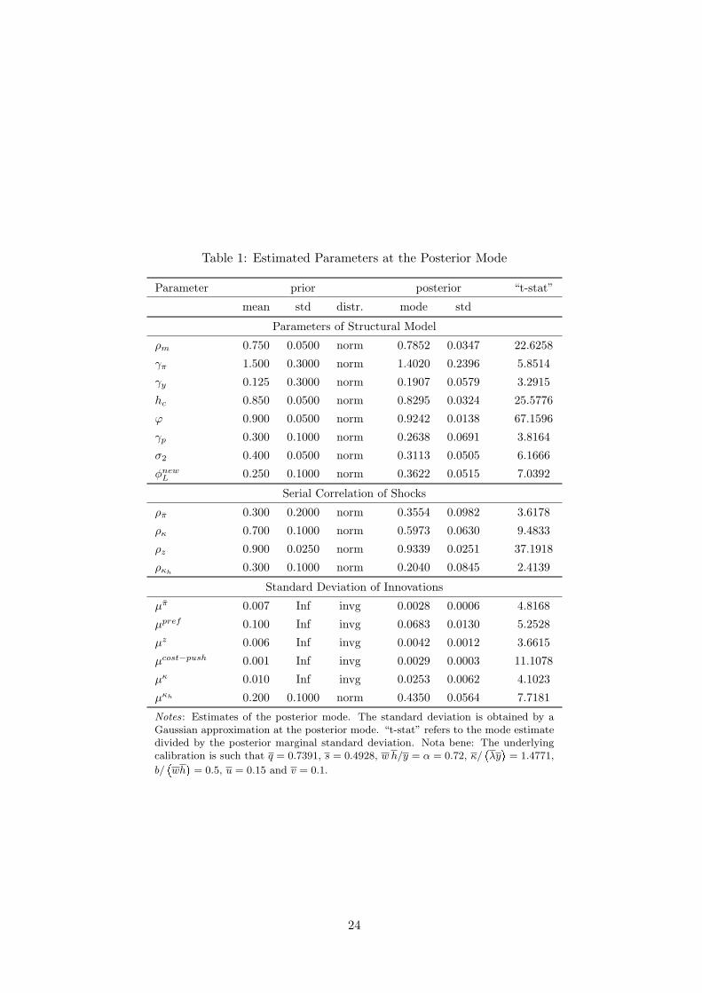
Table 1: Estimated Parameters at the Posterior Mode

Parameter prior posterior “t-stat”

mean std distr. mode std

Parameters of Structural Model

ρm 0.750 0.0500 norm 0.7852 0.0347 22.6258

γπ 1.500 0.3000 norm 1.4020 0.2396 5.8514

γy 0.125 0.3000 norm 0.1907 0.0579 3.2915

hc 0.850 0.0500 norm 0.8295 0.0324 25.5776

ϕ 0.900 0.0500 norm 0.9242 0.0138 67.1596

γp 0.300 0.1000 norm 0.2638 0.0691 3.8164

σ2 0.400 0.0500 norm 0.3113 0.0505 6.1666

φnewL 0.250 0.1000 norm 0.3622 0.0515 7.0392

Serial Correlation of Shocks

ρπ 0.300 0.2000 norm 0.3554 0.0982 3.6178

ρκ 0.700 0.1000 norm 0.5973 0.0630 9.4833

ρz 0.900 0.0250 norm 0.9339 0.0251 37.1918

ρκh0.300 0.1000 norm 0.2040 0.0845 2.4139

Standard Deviation of Innovations

µπ 0.007 Inf invg 0.0028 0.0006 4.8168

µpref 0.100 Inf invg 0.0683 0.0130 5.2528

µz 0.006 Inf invg 0.0042 0.0012 3.6615

µcost−push 0.001 Inf invg 0.0029 0.0003 11.1078

µκ 0.010 Inf invg 0.0253 0.0062 4.1023

µκh 0.200 0.1000 norm 0.4350 0.0564 7.7181

Notes: Estimates of the posterior mode. The standard deviation is obtained by aGaussian approximation at the posterior mode. “t-stat” refers to the mode estimatedivided by the posterior marginal standard deviation. Nota bene: The underlyingcalibration is such that q = 0.7391, s = 0.4928, w h/y = α = 0.72, κ/

�λy

�= 1.4771,

b/�wh

�= 0.5, u = 0.15 and v = 0.1.

24

(2005), Eichenbaum and Fisher (2003) and Kuester (2006), for instance. We seek to explore this

in future research. We find a low degree of price indexation, γp = 0.26. Finally, the weight on

unemployment in the matching process is estimated to be well below half, σ2 = 0.31. New matches

in Germany according to our model estimates are driven by vacancies rather than by the pool of

unemployed workers in contrast to the estimates of Burda and Wyplosz (1994) until 1991.

Turning to shock persistence, our results seem in line with the literature. Worth mentioning is

that labor market friction shocks (vacancy posting shocks) are estimated to be less persistent

than the prior mean, ρκ = 0.6. Persistent shocks to the labor market do not explain persistence

in labor market movements in our model. The innovation to the disutility of work, µκh , does

not match well with the prior. Its posterior value is 0.44, well above its prior mean and, from

an economic perspective, at the border of being reasonable. Otherwise posterior mode estimates

of innovations appear to be reasonable. Introducing the extensive margin into the macro-model

helps reconciliate macro and micro evidence without compromising on fit.

As a measure of matching data properties, Table 2 reports how well the standard deviations of

the endogenous variables in our model match with the time-series evidence. To that aim, we

Table 2: Model Second Moments Relative to Data

Variable RMSE (model) RMSE (VAR) std (model) std (data) std (VAR)

yt 1.09 0.96 1.67 1.73 1.66

rt 0.09 0.08 0.36 0.44 0.37

πannt 0.37 0.40 1.47 1.32 1.10

nt 0.43 0.38 0.85 1.09 1.03

wt 0.62 0.58 2.39 2.23 1.65

Notes: All entries have been multiplied by 100. The table compares the root mean squaredforecast error of the model evaluated at the posterior mode (second column) to the root meansquared forecast errors resulting from a VAR(2) in the sample 1984:3 - 2004:2 (third column).The fourth to sixth column compare the standard deviations implied by the model to those takendirectly from the data and those taken from an auxiliary VAR(2). Nota bene: standard deviationof hours (very dependent on the choice of the data series): 0.0210 (model) vs. 0.05328(data);standard deviation of vacancies: 0.0817 (model) vs. 0.3016(data)

compare the model standard deviations to those taken directly from the data and those taken

from an auxiliary VAR(2) model. Overall, our model seems to fit the second moments of the data

rather well. When it comes to comparing root mean squared forecast errors, only the consumption

equation falls behind a VAR(2) in terms of forecast performance. That the model explains the

25

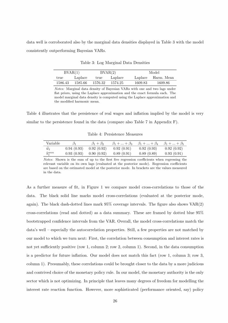
data well is corroborated also by the marginal data densities displayed in Table 3 with the model

consistently outperforming Bayesian VARs.

Table 3: Log Marginal Data Densities

BVAR(1) BVAR(2) Model

true Laplace true Laplace Laplace Harm. Mean

1586.43 1585.66 1576.32 1574.25 1609.83 1609.86

Notes: Marginal data density of Bayesian VARs with one and two lags underflat priors, using the Laplace approximation and the exact formula each. Themodel marginal data density is computed using the Laplace approximation andthe modified harmonic mean.

Table 4 illustrates that the persistence of real wages and inflation implied by the model is very

similar to the persistence found in the data (compare also Table 7 in Appendix F).

Table 4: Persistence Measures

Variable β1 β1 + β2 β1 + ...+ β3 β1 + ...+ β4 β1 + ...+ β5

wt 0.94 (0.93) 0.92 (0.92) 0.92 (0.91) 0.92 (0.93) 0.92 (0.92)

πannt 0.93 (0.93) 0.90 (0.92) 0.89 (0.91) 0.89 (0.89) 0.93 (0.91)

Notes: Shown is the sum of up to the first five regression coefficients when regressing therelevant variable on its own lags (evaluated at the posterior mode). Regression coefficientsare based on the estimated model at the posterior mode. In brackets are the values measuredin the data.

As a further measure of fit, in Figure 1 we compare model cross-correlations to those of the

data. The black solid line marks model cross-correlations (evaluated at the posterior mode,

again). The black dash-dotted lines mark 95% coverage intervals. The figure also shows VAR(2)

cross-correlations (read and dotted) as a data summary. These are framed by dotted blue 95%

bootstrapped confidence intervals from the VAR. Overall, the model cross-correlations match the

data’s well – especially the autocorrelation properties. Still, a few properties are not matched by

our model to which we turn next: First, the correlation between consumption and interest rates is

not yet sufficiently positive (row 1, column 2; row 2, column 1). Second, in the data consumption

is a predictor for future inflation. Our model does not match this fact (row 1, column 3; row 3,

column 1). Presumably, these correlations could be brought closer to the data by a more judicious

and contrived choice of the monetary policy rule. In our model, the monetary authority is the only

sector which is not optimizing. In principle that leaves many degrees of freedom for modelling the

interest rate reaction function. However, more sophisticated (performance oriented, say) policy

26

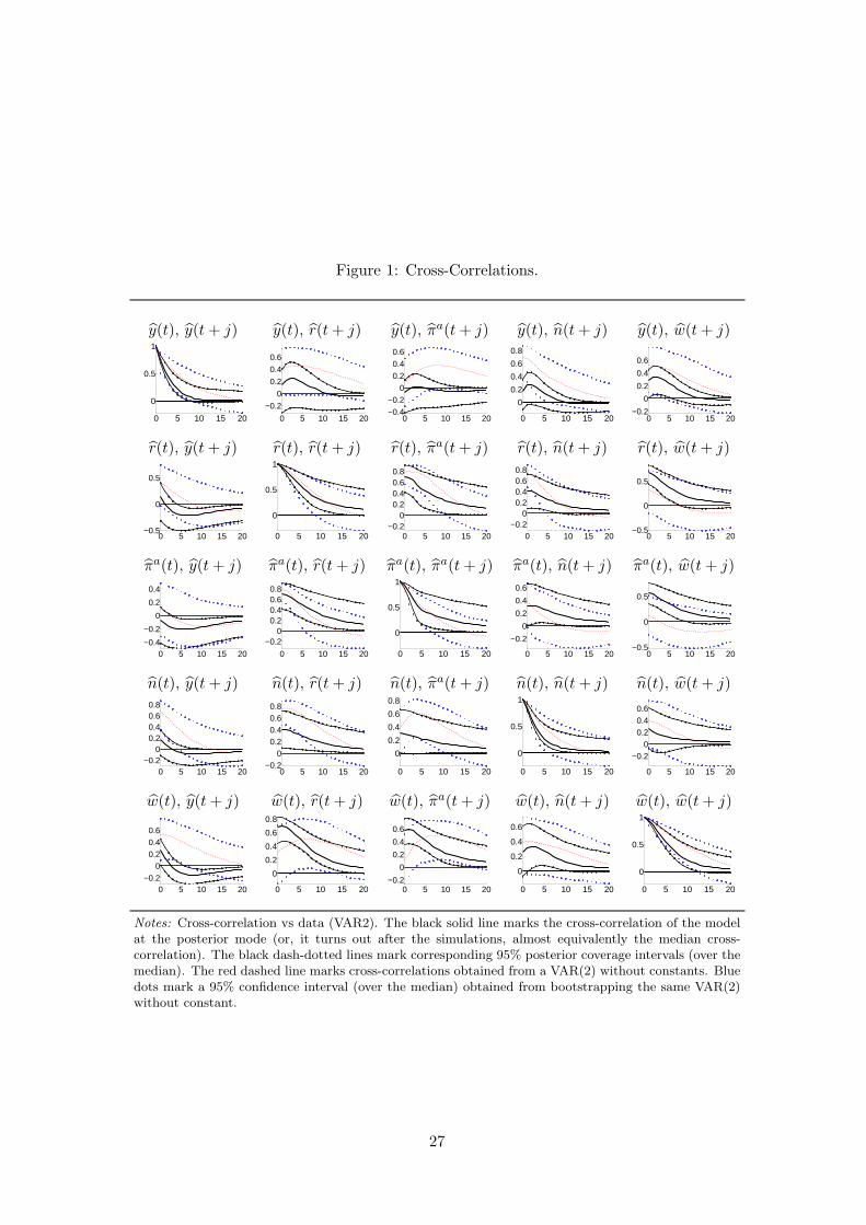
Figure 1: Cross-Correlations.

y(t), y(t+ j) y(t), r(t+ j) y(t), πa(t+ j) y(t), n(t+ j) y(t), w(t+ j)

0 5 10 15 20

0

0.5

1

0 5 10 15 20

−0.2

0

0.2

0.4

0.6

0 5 10 15 20−0.4−0.2

00.20.40.6

0 5 10 15 20

0

0.2

0.4

0.6

0.8

0 5 10 15 20−0.2

0

0.2

0.4

0.6

r(t), y(t+ j) r(t), r(t+ j) r(t), πa(t+ j) r(t), n(t+ j) r(t), w(t+ j)

0 5 10 15 20−0.5

0

0.5

0 5 10 15 20

0

0.5

1

0 5 10 15 20−0.2

00.20.40.60.8

0 5 10 15 20−0.2

00.20.40.60.8

0 5 10 15 20−0.5

0

0.5

πa(t), y(t+ j) πa(t), r(t+ j) πa(t), πa(t+ j) πa(t), n(t+ j) πa(t), w(t+ j)

0 5 10 15 20−0.4

−0.2

0

0.2

0.4

0 5 10 15 20

−0.20

0.20.40.60.8

0 5 10 15 20

0

0.5

1

0 5 10 15 20

−0.2

0

0.2

0.4

0.6

0 5 10 15 20−0.5

0

0.5

n(t), y(t+ j) n(t), r(t+ j) n(t), πa(t+ j) n(t), n(t+ j) n(t), w(t+ j)

0 5 10 15 20−0.2

00.20.40.60.8

0 5 10 15 20−0.2

00.20.40.60.8

0 5 10 15 20

0

0.2

0.4

0.6

0.8

0 5 10 15 20

0

0.5

1

0 5 10 15 20

−0.20

0.20.40.6

w(t), y(t+ j) w(t), r(t+ j) w(t), πa(t+ j) w(t), n(t+ j) w(t), w(t+ j)

0 5 10 15 20−0.2

00.20.40.6

0 5 10 15 20

0

0.2

0.4

0.6

0.8

0 5 10 15 20−0.2

0

0.2

0.4

0.6

0 5 10 15 20

0

0.2

0.4

0.6

0 5 10 15 20

0

0.5

1

Notes: Cross-correlation vs data (VAR2). The black solid line marks the cross-correlation of the modelat the posterior mode (or, it turns out after the simulations, almost equivalently the median cross-correlation). The black dash-dotted lines mark corresponding 95% posterior coverage intervals (over themedian). The red dashed line marks cross-correlations obtained from a VAR(2) without constants. Bluedots mark a 95% confidence interval (over the median) obtained from bootstrapping the same VAR(2)without constant.

27

rules may tend to overfit – making policy-analysis on the basis of the model a dubious task. We

prefer to stick to the parsimonious Taylor rule. Third, both employment and the real wage are

not sufficiently positively correlated with future output (rows 4 and 5, column 1).

We have pointed out some short-comings. By and large, we conclude, nevertheless, that the model

does a good job at fitting the data. We next turn to the propagation mechanism of shocks and

ultimately to the policy considerations.

28

5 The Impact of the Labor Market on Model Dynamics

In this section, we analyze the dynamics of the estimated model. Towards that aim, we present

empirical impulse response functions as well as forecast error variance decompositions. In particu-

lar, we investigate the specific role of the labor market for the model’s dynamics. Additionally, we

will present counterfactual scenarios illustrating the dynamics of the economy in different labor

market regimes.

In a first step, we are particularly interested in how a monetary policy shock is transmitted in the

presence of a rigid non-Walrasian labor market in a stable monetary environment. An increase

in the inflation target in our model corresponds to the central bank decreasing its key interest

rate (see the solid line in Figure 2). The lowered rate reduces savings and increases household

consumption. The increased demand in turn requires additional labor input. Due to the rigidities

in the labor market the number of employed workers cannot be increased instantly.24 Hence labor

adjustment is initially implemented via an increase of hours worked per employee. The increased

demand boosts expected profits and vacancy posting increases until expected profits equal the

posting costs. In anticipation of higher profits the value of an employment relation increases and

workers aspire higher wages. Firms’ marginal cost of production increase with higher wage rates

implying higher prices and higher inflation (see Figure 2).

Figure 2 also shows a counterfactual exercise illustrating the effect of wage rigidity.25 We compare

the response to an inflation target shock in the estimated model with the response in a model

assuming flexible wages.26 Given full wage flexibility, profits increase more sharply after a mone-

tary policy shock which leads to a correspondingly more pronounced increase in real wages. This

in turn triggers a stronger response of inflation compared to the benchmark model with rigid

wages. Therefore, introducing wage rigidity in the right-to-manage model smoothes wages as well

as marginal cost so that the wage induced inertia in marginal costs translates into more persistent

24 Although this would be beneficial due to decreasing returns to labor.

25 A detailed description of all the counterfactual exercises can be found in Appendix F.

26 The red dotted line marked by triangles in Figure 2 shows the impulse responses when wage rigidity is eliminated.Towards that aim, we set the wage adjustment cost parameter φnew

L to zero.

29

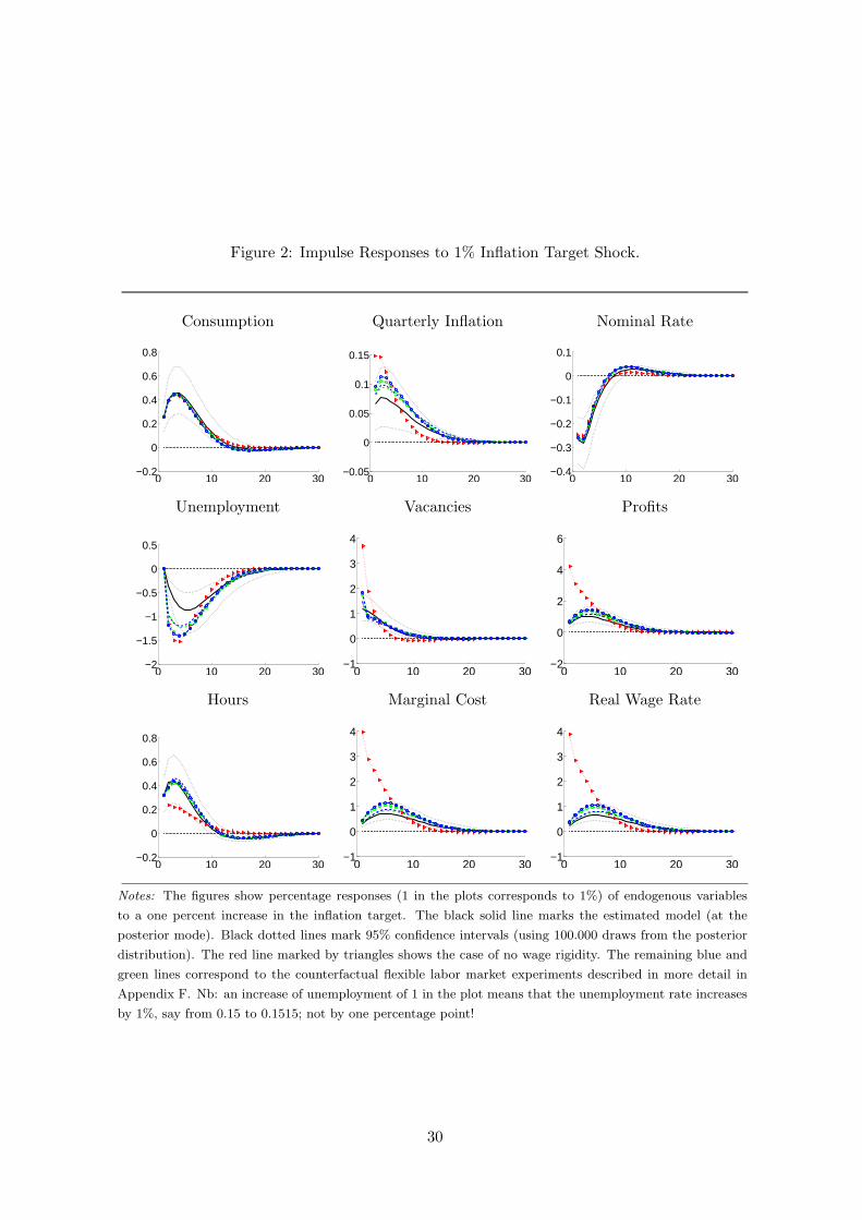
Figure 2: Impulse Responses to 1% Inflation Target Shock.

Consumption Quarterly Inflation Nominal Rate

0 10 20 30−0.2

0

0.2

0.4

0.6

0.8

0 10 20 30−0.05

0

0.05

0.1

0.15

0 10 20 30−0.4

−0.3

−0.2

−0.1

0

0.1

Unemployment Vacancies Profits

0 10 20 30−2

−1.5

−1

−0.5

0

0.5

0 10 20 30−1

0

1

2

3

4

0 10 20 30−2

0

2

4

6

Hours Marginal Cost Real Wage Rate

0 10 20 30−0.2

0

0.2

0.4

0.6

0.8

0 10 20 30−1

0

1

2

3

4

0 10 20 30−1

0

1

2

3

4

Notes: The figures show percentage responses (1 in the plots corresponds to 1%) of endogenous variables

to a one percent increase in the inflation target. The black solid line marks the estimated model (at the

posterior mode). Black dotted lines mark 95% confidence intervals (using 100.000 draws from the posterior

distribution). The red line marked by triangles shows the case of no wage rigidity. The remaining blue and

green lines correspond to the counterfactual flexible labor market experiments described in more detail in

Appendix F. Nb: an increase of unemployment of 1 in the plot means that the unemployment rate increases

by 1%, say from 0.15 to 0.1515; not by one percentage point!

30

inflation via the new Keynesian Phillips curve. In terms of the response of unemployment, more

flexible wages yield a stronger fall of unemployment. In addition, unemployment appears to be

somewhat less persistent than under a regime of rigid wages.27

Additionally, Figure 2 shows the second counterfactual exercise. We compare responses of vari-

ables in the benchmark model to an inflation target shock with the one under a flexible labor

market regime (see the dotted blue and green lines in the figure). The labor market is less rigid

in the following sense: We assume that all workers immediately find a job in steady state, which

corresponds to an abundance of firms in the market. We do, however, retain the wage rigidity.

An increase in the inflation target decreases the real interest rate leading to an increase in con-

sumption. Hence profits rise and vacancies increase accordingly. In a more flexible labor market

regime, labor market tightness is affected more by movements in unemployment. This in turn

translates into larger movements in wages and also inflation than in the rigid baseline. Therefore,

we conclude that more rigid labor markets, especially when rigidities lie on the wage side, lead to

more persistent movements in inflation. This implies that the transmission mechanism of mone-

tary policy is influenced by the degree of rigidities in the labor market – and that the latter are

of first-order importance for the way monetary policy needs to be conducted.

In a second step, we look directly at shocks originating in the labor market. Towards that

aim, we proxy labor market impediments by the cost of vacancy posting. We analyze how a

shock to vacancy posting affects the nominal and real variables in our model (see the solid black

line in Figure 3. In our simulations, a vacancy posting cost shock increases the cost of posting

a vacancy by 1%. Vacancy posting activity decreases but the job destruction rate remaining

constant by assumption. Hence unemployment increases. Hours worked need to increase to

satisfy consumption demand. Consumption itself is affected only slightly due to the assumption

of strong habits and income pooling. Rising job creation costs augment the value of existing

employment relations which leads to a rise in wages and profits, and ultimately inflation.

Figure 3 also shows the response of the variables to a vacancy posting cost shock under a flexible

27 Notice that due to income pooling the labor market dynamics do not translate into changes in the behavior ofconsumption.

31

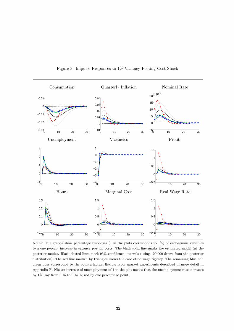
Figure 3: Impulse Responses to 1% Vacancy Posting Cost Shock.

Consumption Quarterly Inflation Nominal Rate

0 10 20 30−0.03

−0.02

−0.01

0

0.01

0 10 20 30−0.01

0

0.01

0.02

0.03

0.04

0 10 20 30−5

0

5

10

15

20x 10−3

Unemployment Vacancies Profits

0 10 20 30−1

0

1

2

3

0 10 20 30−4

−3

−2

−1

0

1

0 10 20 30−0.5

0

0.5

1

1.5

Hours Marginal Cost Real Wage Rate

0 10 20 30−0.1

0

0.1

0.2

0.3

0 10 20 30−0.5

0

0.5

1

1.5

0 10 20 30−0.5

0

0.5

1

1.5

Notes: The graphs show percentage responses (1 in the plots corresponds to 1%) of endogenous variables

to a one percent increase in vacancy posting costs. The black solid line marks the estimated model (at the

posterior mode). Black dotted lines mark 95% confidence intervals (using 100.000 draws from the posterior

distribution). The red line marked by triangles shows the case of no wage rigidity. The remaining blue and

green lines correspond to the counterfactual flexible labor market experiments described in more detail in

Appendix F. Nb: an increase of unemployment of 1 in the plot means that the unemployment rate increases

by 1%, say from 0.15 to 0.1515; not by one percentage point!

32

wage regime. An increase in vacancy posting costs depresses vacancy postings as before. Profits of

operating firms rise to a greater extent than in the baseline. Higher profits in turn lead to higher

wages and higher marginal costs translating into an increased response of inflation. Consequently,

that means that vacancies experience a smaller drop and unemployment rises by less than in the

benchmark.

Closely watching labor market developments could be important for monetary policy makers if

these developments ultimately have an effect on inflation and consumption and if the traditional

New Keynesian variables are not sufficient statistics in this respect. The variance decomposition in

Table 5 shows how much of the forecast error variance in each variable at different forecast horizons

is due to a specific set of innovations. Corroborating the variance decomposition evidence in Table

5, we report actual error decompositions (after running the Kalman-Smoother) at business cycle

frequencies in Figure 10 (Appendix E).

The vacancy posting cost shock is the key driving force of employment (87% in the short-run

and 63% in the long run) and vacancies (roughly 80% in the short and long-run). It is also an

important determinant for wages, hours worked and marginal cost (roughly 10% to 15% in the

short and long run) but with not enough transmission to let it matter for inflation or consumption.

As is apparent from Table 5 less than 5 percent of the variation of inflation, output and interest

rates is driven by labor market shocks. This result holds at all frequencies.We can conclude that

the impact of shocks to vacancy posting on nominal and real variables of the model is rather

limited.

Finally, we take a closer look at the labor market itself. We see that besides the vacancy posting

cost shock and the disutility of work shock, labor market variables are especially influenced by

technology and demand shocks. In contrast, the inflation target shock and the cost push shock

are irrevelant for labor market fluctuations.28 In general, unsystematic monetary policy is not a

suspect for being an important determinant of fluctuations in the labor market.

28 The inflation target shock is rather important for interest rate fluctuations determining 50% of its fluctuationsin the short run and 14% in the long run. The cost push shock mainly drives the inflation rate and hardly spillsover to other variables (apart from interest rates). It explains 88% of inflation variations in the short-run andstill 38% in the long-run.

33

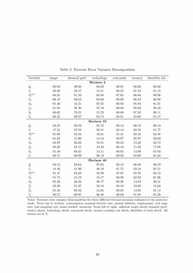
Table 5: Forecast Error Variance Decomposition

Variable target demand pref. technology cost-push vacancy disutility lab.

Horizon 2

yt 00.89 99.08 00.02 00.01 00.00 00.00

rt 50.39 28.57 12.41 06.25 01.24 01.15

πannt 00.35 01.50 08.68 87.65 00.86 00.96

nt 00.19 08.62 03.69 00.00 86.52 00.99

wt 01.46 24.31 07.05 00.04 05.83 61.31

xt 01.02 28.36 37.18 00.02 05.02 28.40

ht 00.62 79.25 12.70 00.00 07.32 00.11

vt 00.32 09.87 04.74 00.01 83.90 01.17

Horizon 10

yt 03.25 93.59 02.72 00.13 00.18 00.13

rt 17.55 37.84 38.21 02.14 02.50 01.77

πannt 01.60 04.34 43.01 45.41 03.16 02.48

nt 01.62 15.80 14.53 00.07 65.97 02.02

wt 04.97 30.03 16.81 00.24 15.20 32.74

xt 03.26 24.15 44.33 00.16 11.02 17.08

ht 01.48 69.45 13.11 00.05 14.90 01.03

vt 00.57 09.99 06.13 00.02 82.09 01.20

Horizon 40

yt 03.12 88.64 07.65 00.13 00.28 00.19

rt 14.46 31.99 48.10 01.75 02.19 01.51

πannt 01.47 03.68 52.29 37.67 02.76 02.12

nt 01.75 15.19 18.17 00.09 62.85 01.96

wt 05.39 28.33 20.77 00.28 14.83 30.41

xt 03.26 21.37 50.16 00.16 10.00 15.04

ht 01.49 69.33 13.05 00.05 14.95 01.14

vt 00.57 09.97 06.38 00.02 81.85 01.20

Notes: Forecast error variance demcoposition for three different forecast horizons evaluated at the posteriormode. From top to bottom: consumption, nominal interest rate, annual inflation, employment, real wagerate, real marginal cost, hours worked, vacancies. From left to right: inflation target shock, demand (pref-erence) shock, technology shock, cost-push shock, vacancy posting cost shock, disutility of work shock. Allentries are in %.

34

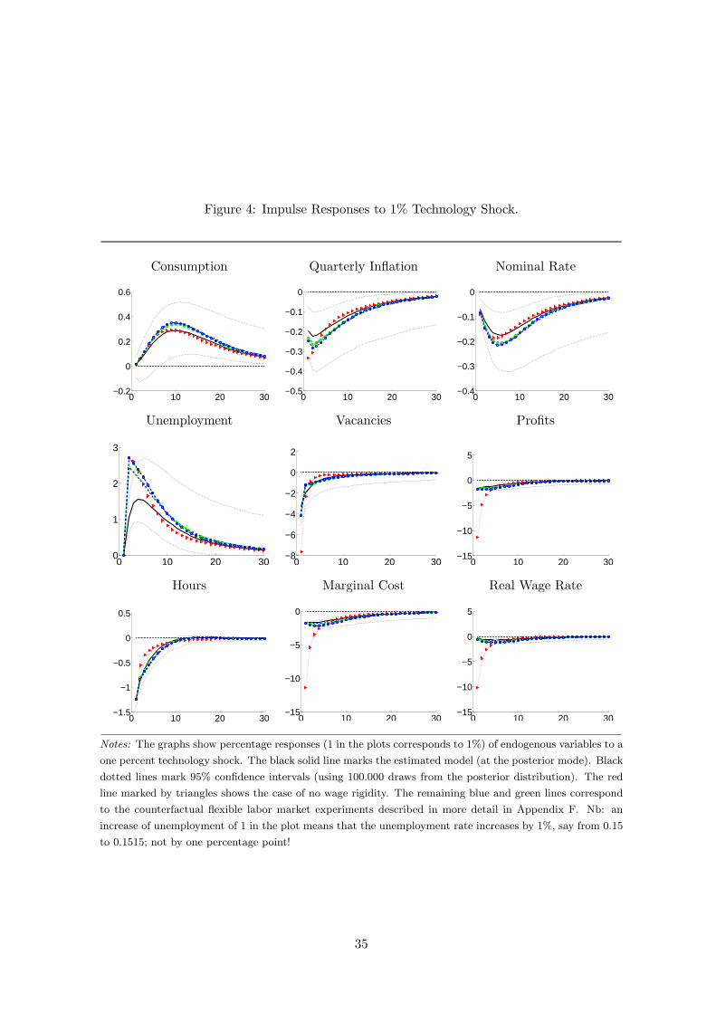
Figure 4: Impulse Responses to 1% Technology Shock.

Consumption Quarterly Inflation Nominal Rate

0 10 20 30−0.2

0

0.2

0.4

0.6

0 10 20 30−0.5

−0.4

−0.3

−0.2

−0.1

0

0 10 20 30−0.4

−0.3

−0.2

−0.1

0

Unemployment Vacancies Profits

0 10 20 300

1

2

3

0 10 20 30−8

−6

−4

−2

0

2

0 10 20 30−15

−10

−5

0

5

Hours Marginal Cost Real Wage Rate

0 10 20 30−1.5

−1

−0.5

0

0.5

0 10 20 30−15

−10

−5

0

0 10 20 30−15

−10

−5

0

5

Notes: The graphs show percentage responses (1 in the plots corresponds to 1%) of endogenous variables to a

one percent technology shock. The black solid line marks the estimated model (at the posterior mode). Black

dotted lines mark 95% confidence intervals (using 100.000 draws from the posterior distribution). The red

line marked by triangles shows the case of no wage rigidity. The remaining blue and green lines correspond

to the counterfactual flexible labor market experiments described in more detail in Appendix F. Nb: an

increase of unemployment of 1 in the plot means that the unemployment rate increases by 1%, say from 0.15

to 0.1515; not by one percentage point!

35

The Keynesian nature of our model becomes most apparent when examining the effect of a positive

technology shock (see Figure 4). Hours worked fall as less labor input is required to produce

the demand determined output.29 This reinforces the increase in the marginal product of labor

caused by the technology shock. In addition, the marginal dis-utility of work falls, reducing the

real wage rate. Marginal cost fall driven by both the falling wage rate and the increased marginal

product of labor. Inflation falls accordingly. The associated interest rate reductions via the central

bank reaction function increase consumption gradually. Expected profits are tightly linked to the

dynamics in hours and wages. Therefore, lower wages and hours come along with lower profits and

hence reduced vacancy posting intensity. This causes a rise in unemployment. The autocorrelated

technology shock imposes a significant degree of persistence on the real and nominal variables.

In terms of the variance decomposition, the technology shock is a key determinant of marginal cost

(determining 37% of its fluctuations in the short and 50% in the long run). Hence productivity

fluctuations in our model are very important for inflation, determining 12% of its variability in the

short-run and more than half in the long-run. In the long run, technology also plays an important

role for real wage and consumption fluctuations. The figures are 20% and 8%, respectively.

The preference shock stimulates current consumption (see Figure 5). The increased demand re-

quires additional labor input which initially is fully provided by an extension of hours worked.

Higher expected profits translate into more vacancy posting and hence into an increase in employ-

ment. The demand shock induces a positive correlation between all main variables as it is found

in the German data (compare Table 8 for the cross correlations in the data).

Looking at the variance decomposition, it appears that the demand shock drives all consumption

movement in the short run and still 89% in the long run. It explains roughly 30% of real wage

movements and marginal cost. And, indeed as we have argued above, there are other shocks which

have more influence on marginal cost and thus on inflation. The demand shock is not a strong

driving force of inflation: not more than 5% of the forecast error variance of inflation fall on the

demand shock.

29 The response of hours worked to technology shocks recently has caused an intense discussion in the profession.The fall of hours worked in response to a technology shock is in line with evidence reported in Gali (1999) andFrancis and Ramey (2002), for instance.

36

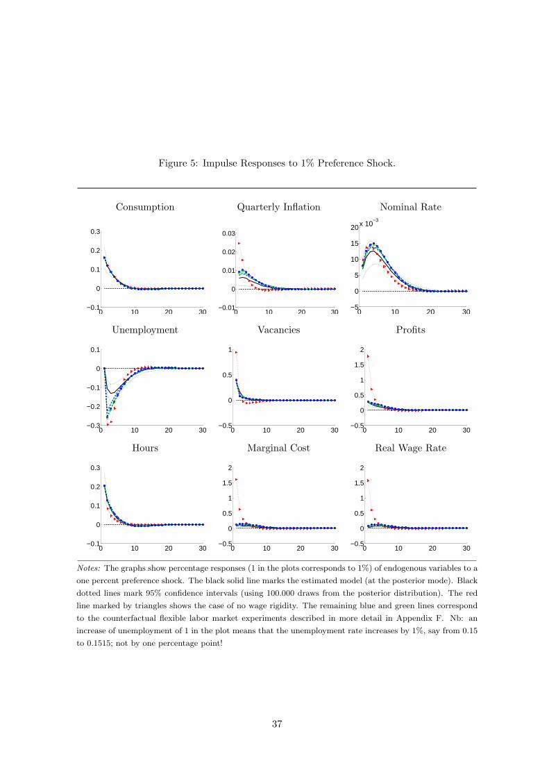
Figure 5: Impulse Responses to 1% Preference Shock.

Consumption Quarterly Inflation Nominal Rate

0 10 20 30−0.1

0

0.1

0.2

0.3

0 10 20 30−0.01

0

0.01

0.02

0.03

0 10 20 30−5

0

5

10

15

20x 10−3

Unemployment Vacancies Profits

0 10 20 30−0.3

−0.2

−0.1

0

0.1

0 10 20 30−0.5

0

0.5

1

0 10 20 30−0.5

0

0.5

1

1.5

2

Hours Marginal Cost Real Wage Rate

0 10 20 30−0.1

0

0.1

0.2

0.3

0 10 20 30−0.5

0

0.5

1

1.5

2

0 10 20 30−0.5

0

0.5

1

1.5

2

Notes: The graphs show percentage responses (1 in the plots corresponds to 1%) of endogenous variables to a

one percent preference shock. The black solid line marks the estimated model (at the posterior mode). Black

dotted lines mark 95% confidence intervals (using 100.000 draws from the posterior distribution). The red

line marked by triangles shows the case of no wage rigidity. The remaining blue and green lines correspond

to the counterfactual flexible labor market experiments described in more detail in Appendix F. Nb: an

increase of unemployment of 1 in the plot means that the unemployment rate increases by 1%, say from 0.15

to 0.1515; not by one percentage point!

37

In brief, our results show that the labor market helps to understand the transmission of monetary

policy on inflation. Our counterfactual exercises display that the more rigid the labor market,

and particularly the real wage is, the more persistent is the response of inflation to an inflation

target shock. Moreover, we can show that labor market shocks translate only marginally into the

dynamics of nominal variables variables in the model – raising doubt whether shocks originating

in the labor market are important information for monetary policy.

38

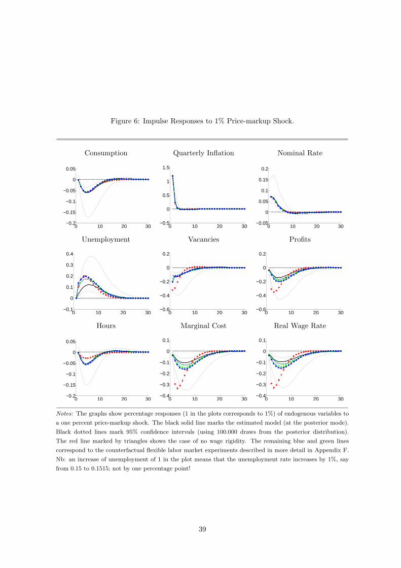
Figure 6: Impulse Responses to 1% Price-markup Shock.

Consumption Quarterly Inflation Nominal Rate

0 10 20 30−0.2

−0.15

−0.1

−0.05

0

0.05

0 10 20 30−0.5

0

0.5

1

1.5

0 10 20 30−0.05

0

0.05

0.1

0.15

0.2

Unemployment Vacancies Profits

0 10 20 30−0.1

0

0.1

0.2

0.3

0.4

0 10 20 30−0.6

−0.4

−0.2

0

0.2

0 10 20 30−0.6

−0.4

−0.2

0

0.2

Hours Marginal Cost Real Wage Rate

0 10 20 30−0.2

−0.15

−0.1

−0.05

0

0.05

0 10 20 30−0.4

−0.3

−0.2

−0.1

0

0.1

0 10 20 30−0.4

−0.3

−0.2

−0.1

0

0.1

Notes: The graphs show percentage responses (1 in the plots corresponds to 1%) of endogenous variables to

a one percent price-markup shock. The black solid line marks the estimated model (at the posterior mode).

Black dotted lines mark 95% confidence intervals (using 100.000 draws from the posterior distribution).

The red line marked by triangles shows the case of no wage rigidity. The remaining blue and green lines

correspond to the counterfactual flexible labor market experiments described in more detail in Appendix F.

Nb: an increase of unemployment of 1 in the plot means that the unemployment rate increases by 1%, say

from 0.15 to 0.1515; not by one percentage point!

39

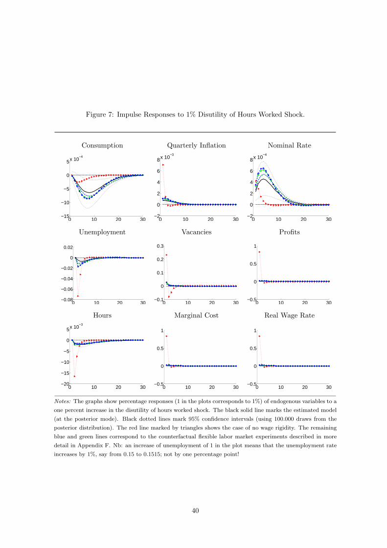
Figure 7: Impulse Responses to 1% Disutility of Hours Worked Shock.

Consumption Quarterly Inflation Nominal Rate

0 10 20 30−15

−10

−5

0

5x 10−4

0 10 20 30−2

0

2

4

6

8x 10−3

0 10 20 30−2

0

2

4

6

8x 10−4

Unemployment Vacancies Profits

0 10 20 30−0.08

−0.06

−0.04

−0.02

0

0.02

0 10 20 30−0.1

0

0.1

0.2

0.3

0 10 20 30−0.5

0

0.5

1

Hours Marginal Cost Real Wage Rate

0 10 20 30−20

−15

−10

−5

0

5x 10−3

0 10 20 30−0.5

0

0.5

1

0 10 20 30−0.5

0

0.5

1

Notes: The graphs show percentage responses (1 in the plots corresponds to 1%) of endogenous variables to a

one percent increase in the disutility of hours worked shock. The black solid line marks the estimated model

(at the posterior mode). Black dotted lines mark 95% confidence intervals (using 100.000 draws from the

posterior distribution). The red line marked by triangles shows the case of no wage rigidity. The remaining

blue and green lines correspond to the counterfactual flexible labor market experiments described in more

detail in Appendix F. Nb: an increase of unemployment of 1 in the plot means that the unemployment rate

increases by 1%, say from 0.15 to 0.1515; not by one percentage point!

40

6 Conclusions

In this paper we estimate a small-scale DSGE model with search and matching frictions by

Bayesian full-information techniques. We focus on a quantitative assessment of the role of la-

bor markets in a stable monetary policy regime. Towards that aim we use German data in order

to avoid possible problems with regard to the heterogeneity of labor market and monetary policy

regimes across the euro area in pre-EMU years.

To account for wage and inflation persistence we model quadratic wage adjustment costs in the

search and matching framework. Using a set of structural shocks including a labor market specific

shock we are able to present evidence on the relative importance of specific disturbances. Fur-

thermore we assess the role of labor market rigidities for monetary policy by counterfactual policy

simulations.

Our results can be summarized as follows. First, we find that the structure of the labor market

matters substantially for the overall behavior of the model and the transmission of monetary policy

on inflation in particular. The specific settings of the labor market, as for example the degree of

wage inertia or the efficiency of the matching process, are found to have a notable impact. The

influence of the labor market is stronger for inflation than for aggregate demand. Specifically, we

find that the degree of wage rigidity is positively correlated with inflation persistence. In addition,

if the frictions associated with finding a new job are sizeable, our results show that the effects of

shocks on inflation last longer. Furthermore we find that a higher degree of wage rigidity amplifies

real adjustment in the labor market and leads to more fluctuations in employment.

Second, the realization of labor market shocks has an impact on the labor market itself but

a limited influence on the other blocks of the model. Therefore labor market shocks do not

contribute much to the cyclical dynamics of non-labor market variables – particularly inflation

– suggesting that the model does not feature much transmission from labor markets to the rest

of the economy. Natural candidates in the modeling structure to introduce further transmission

include the easing of the assumption of perfect consumption insurance and more closely tying

price-setting decisions to decisions in the labor market like hiring and wage-setting.

41

In total, to the extent a central bank’s task is to keep inflation low (and stable) policy makers

need to have a good understanding of the structure of the labor-market. The realization of labor

market specific shocks, however, does not appear to contain important information for the conduct

of monetary policy. We leave a closer examination of this point for future research.

42

References

Abel, A. (1990): “Asset Prices under Habit Formation and Catching Up with the Joneses,”

American Economic Review, Papers and Proceedings, 80, 38–42.

Altig, D., L. J. Christiano, M. Eichenbaum, and J. Linde (2005): “Firm-Specific Capital,

Nominal Rigidities and the Business Cycle,” .

Bachmann, R. (2005): “Labour Market Dynamics in Germany: Hirings, Separations, and Job-to-

Job Transitions over the Business Cycle,” Humboldt University: SFB Discussion Paper 2005-45.

Boldrin, M., L. Christiano, and J. Fisher (2001): “Habit Persistence, Asset Returns and

the Business Cycle,” American Economic Review, 91(1), 149–166.

Braun, H. (2005): “(Un)employment Dynamics: The Case of Monetary Policy Shocks,” mimeo;

Northwestern University.

Burda, M., and C. Wyplosz (1994): “Gross Worker and Job Flows in Europe,” European

Economic Review, 38(6), 1287–1315.

Calvo, G. (1983): “Staggered Prices in a Utility Maximizing Framework,” Journal of Monetary

Economics, 12, 383–398.

Campbell, J., A. Lo, and C. MacKinlay (1997): The Econometrics of Financial Markets.

Princeton University Press, Princeton.

Christiano, L. J., M. Eichenbaum, and C. Evans (2005): “Nominal Rigiditiesn and the

Dynamic Effects of a Shock to Monetary Policy,” Journal of Political Economy.

Christoffel, K., and T. Linzert (2005): “The Role of Real Wage Rigidity and Labor Market

Frictions for Inflation and Unemployment Dynamics,” mimeo.

Clarida, R., J. Gali, and M. Gertler (1998): “Monetary Policy Rules in Practice. Some

International Evidence,” European Economic Review, 42(6), 1033–1067.

del Negro, M., F. Schorfheide, F. Smets, and R. Wouters (2004): “On the Fit and

Forecasting Performance of New Keynesian Models,” Federal Reserve Bank of Atlanta Working

Paper 2004–37.

Eichenbaum, M., and J. Fisher (2003): “Evaluating the Calvo Model of Sticky Prices,” Federal

Reserve Bank of Chicago, Working Paper 2003-23.

Francis, N., and V. A. Ramey (2002): “Is the Technology-Driven Real Business Cycle Hypoth-

esis Dead? Shocks and Aggregate Fluctuations Revisited,” NBER Working Paper No. 8726.

Fuhrer, J. (2000): “Habit Formation in Consumption and Its Implications for Monetary-Policy

Models,” American Economic Review, 90(3), 367–390.

Gali, J. (1999): “Technology, Employment and the Business Cycle: Do Technology Shocks

Explain Aggregate Fluctuations?,” American Economic Review, 89(1), 249–271.

43

Gali, J., M. Gertler, and D. Lopez-Salido (2001): “European Inflation Dynamics,” Euro-

pean Economic Review, 45.

Gertler, M., and A. Trigari (2005): “Unemployment Fluctuations with Staggered Nash Wage

Bargaining,” mimeo; New York University.

Hall, R. (2005): “Employment Fluctuations with Equilibrium Wage Stickiness,” American Eco-

nomic Review, 95(1), 1.

Hoffmann, J., and J.-R. Kurz-Kim (2004): “Consumer Price Adjustment Under the Mi-

croscope: Germany in a Period of Low Inflation,” Unpublished Manuscript; proceeding of the

“Inflation Persistence Network”.

Kuester, K. (2006): “Real Price and Wage Rigidities in a Model with Matching Frictions,”

mimeo, Goethe University Frankfurt.

Lubik, T., and F. Schorfheide (2005): “A Bayesian Look at New Open Economy Models,” .

Mortensen, D., and C. Pissarides (1994): “Job Creation and Job Destruction in the Theory

of Unemployment,” Review of Economic Studies, 61, 397–415.

Schmitt-Grohe, S., and M. Uribe (2004): “Optimal Operational Monetary Policy in the

Christiano-Eichenbaum-Evans Model,” mimeo, Duke University.

Schorfheide, F. (2000): “Loss Function-based Evaluation of DSGE Models,” Journal of Applied

Econometrics, 15(6), 645–670.

Shimer, R. (2004): “The Consequences of Rigid Wages in Search Models,” Journal of the Euro-

pean Economic Association, 2(2).

(2005): “The Cyclical Behavior of Equilibrium Unemployment, Vacancies, and Wages:

Evidence and Theory,” American Economic Review, 95(1), 25–49.

Smets, F., and R. Wouters (2003): “An Estimated Stochastic Dynamic General Equilibrium

Model of the Euro Area,” Journal of European Economic Association, 1(5), 1123–75.

Taylor, J. B. (1993): “Discretion Versus Policy Rules in Practice,” Carnegie-Rochester Confer-

ence Series on Public Policy, 39, 195–214.

Trigari, A. (2004): “Equilibrium Unemployment, Job Flows and Inflation Dynamics,” ECB

Working Paper, 304, –.

Woodford, M. (2003): Interest and Prices: Foundations of a Theory of Monetary Policy. Prince-

ton University Press, Princeton.

44

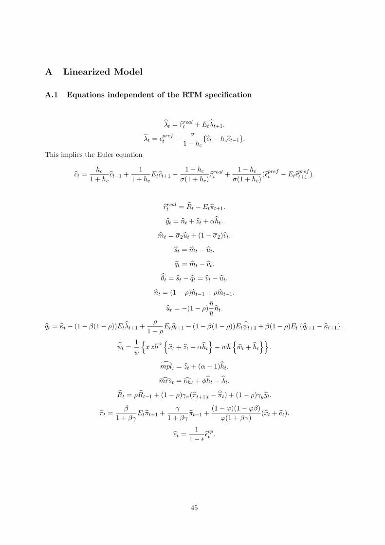
A Linearized Model

A.1 Equations independent of the RTM specification

λt = rrealt + Etλt+1.

λt = ǫpreft −

σ

1 − hc{ct − hcct−1}.

This implies the Euler equation

ct =hc

1 + hcct−1 +

1

1 + hcEtct+1 −

1 − hc

σ(1 + hc)rrealt +

1 − hc

σ(1 + hc)(ǫpref

t − Etǫpreft+1 ).

rrealt = Rt − Etπt+1.

yt = nt + zt + αht.

mt = σ2ut + (1 − σ2)vt.

st = mt − ut.

qt = mt − vt.

θt = st − qt = vt − ut.

nt = (1 − ρ)nt−1 + ρmt−1.

ut = −(1 − ρ)n

unt.

qt = κt − (1− β(1− ρ))Etλt+1 +ρ

1 − ρEtρt+1 − (1− β(1− ρ))Etψt+1 + β(1− ρ)Et {qt+1 − κt+1} .

ψt =1

ψ

{x zh

α{xt + zt + αht

}− wh

{wt + ht

}}.

mplt = zt + (α− 1)ht.

mrst = κht + φht − λt.

Rt = ρRt−1 + (1 − ρ)γπ(πt+1|t − πt) + (1 − ρ)γyyt.

πt =β

1 + βγEtπt+1 +

γ

1 + βγπt−1 +

(1 − ϕ)(1 − ϕβ)

ϕ(1 + βγ)(xt + et).

et =1

1 − ǫǫcpt .

45

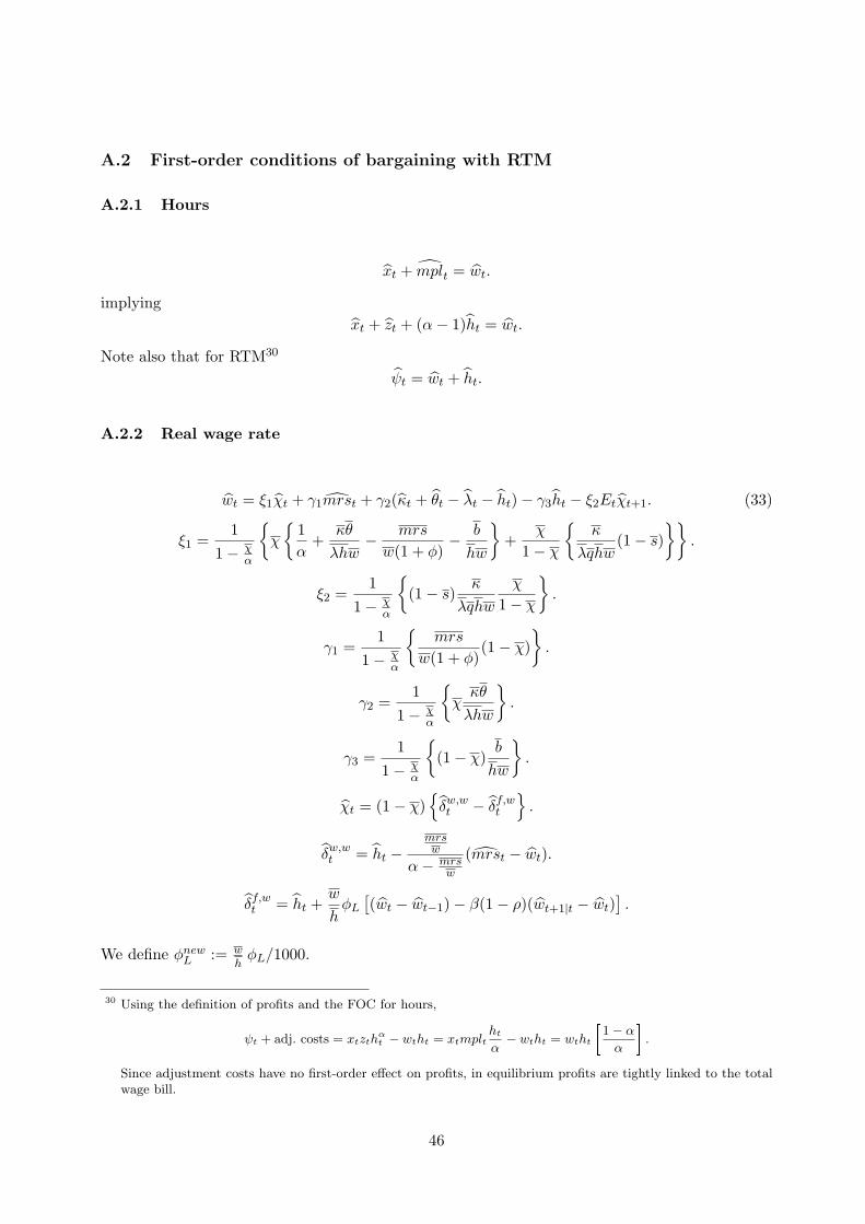
A.2 First-order conditions of bargaining with RTM

A.2.1 Hours

xt + mplt = wt.

implying

xt + zt + (α− 1)ht = wt.

Note also that for RTM30

ψt = wt + ht.

A.2.2 Real wage rate

wt = ξ1χt + γ1mrst + γ2(κt + θt − λt − ht) − γ3ht − ξ2Etχt+1. (33)

ξ1 =1

1 − χα

{χ

{1

α+

κθ

λhw−

mrs

w(1 + φ)−

b

hw

}+

χ

1 − χ

{κ

λqhw(1 − s)

}}.

ξ2 =1

1 − χα

{(1 − s)

κ

λqhw

χ

1 − χ

}.

γ1 =1

1 − χα

{mrs

w(1 + φ)(1 − χ)

}.

γ2 =1

1 − χα

{χκθ

λhw

}.

γ3 =1

1 − χα

{(1 − χ)

b

hw

}.

χt = (1 − χ){δw,wt − δf,w

t

}.

δw,wt = ht −

mrsw

α− mrsw

(mrst − wt).

δf,wt = ht +

w

hφL

[(wt − wt−1) − β(1 − ρ)(wt+1|t − wt)

].

We define φnewL := w

hφL/1000.

30 Using the definition of profits and the FOC for hours,

ψt + adj. costs = xtzthαt − wtht = xtmplt

ht

α− wtht = wtht

�1 − α

α

�.

Since adjustment costs have no first-order effect on profits, in equilibrium profits are tightly linked to the totalwage bill.

46

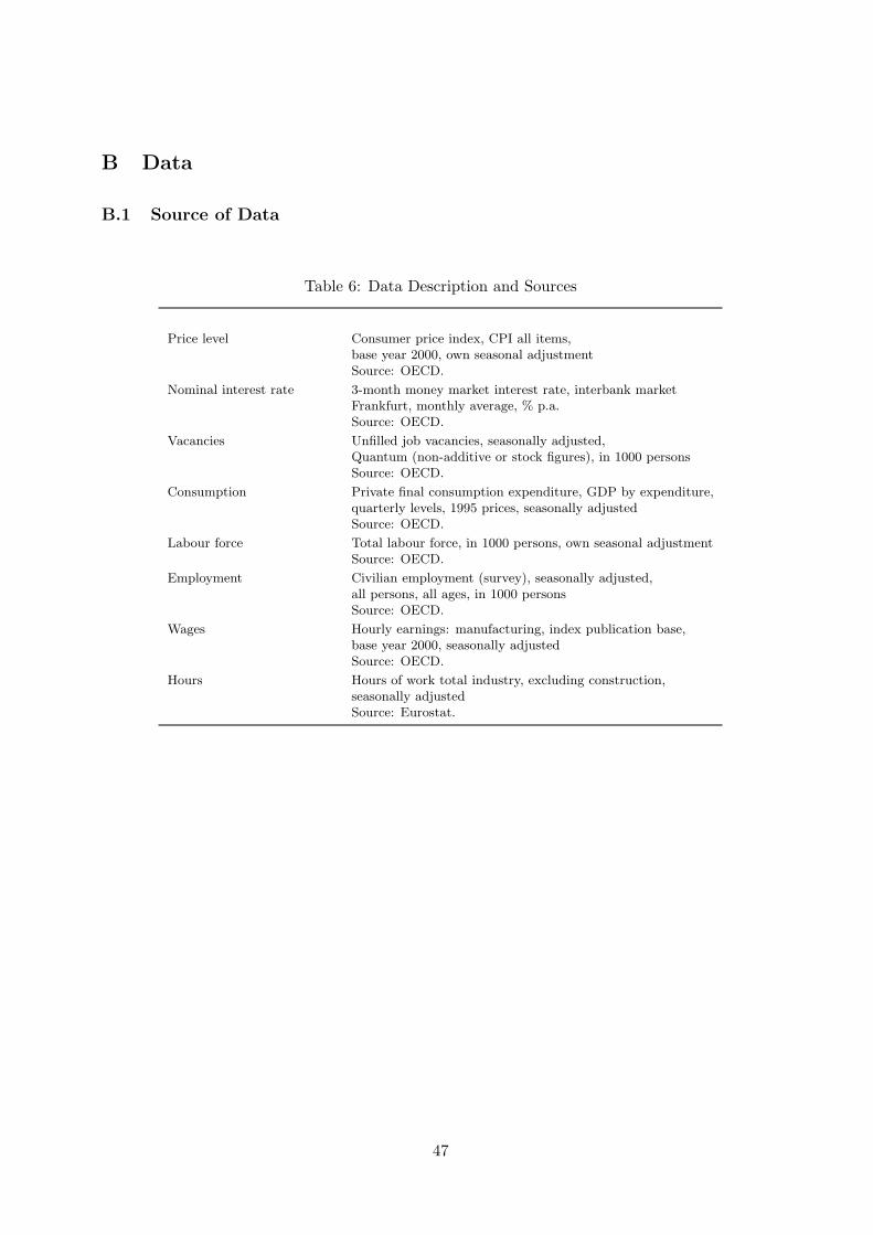
B Data

B.1 Source of Data

Table 6: Data Description and Sources

Price level Consumer price index, CPI all items,base year 2000, own seasonal adjustmentSource: OECD.

Nominal interest rate 3-month money market interest rate, interbank marketFrankfurt, monthly average, % p.a.Source: OECD.

Vacancies Unfilled job vacancies, seasonally adjusted,Quantum (non-additive or stock figures), in 1000 personsSource: OECD.

Consumption Private final consumption expenditure, GDP by expenditure,quarterly levels, 1995 prices, seasonally adjustedSource: OECD.

Labour force Total labour force, in 1000 persons, own seasonal adjustmentSource: OECD.

Employment Civilian employment (survey), seasonally adjusted,all persons, all ages, in 1000 personsSource: OECD.

Wages Hourly earnings: manufacturing, index publication base,base year 2000, seasonally adjustedSource: OECD.

Hours Hours of work total industry, excluding construction,seasonally adjustedSource: Eurostat.

47

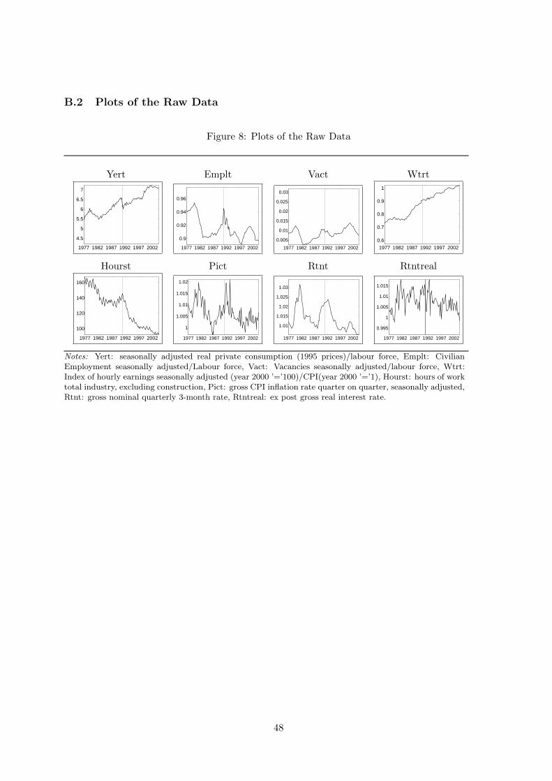
B.2 Plots of the Raw Data

Figure 8: Plots of the Raw Data

Yert Emplt Vact Wtrt

1977 1982 1987 1992 1997 2002

4.5

5

5.5

6

6.5

7

1977 1982 1987 1992 1997 2002

0.9

0.92

0.94

0.96

1977 1982 1987 1992 1997 2002

0.005

0.01

0.015

0.02

0.025

0.03

1977 1982 1987 1992 1997 2002

0.6

0.7

0.8

0.9

1

Hourst Pict Rtnt Rtntreal

1977 1982 1987 1992 1997 2002

100

120

140

160

1977 1982 1987 1992 1997 2002

1

1.005

1.01

1.015

1.02

1977 1982 1987 1992 1997 2002

1.01

1.015

1.02

1.025

1.03

1977 1982 1987 1992 1997 2002

0.995

1

1.005

1.01

1.015

Notes: Yert: seasonally adjusted real private consumption (1995 prices)/labour force, Emplt: CivilianEmployment seasonally adjusted/Labour force, Vact: Vacancies seasonally adjusted/labour force, Wtrt:Index of hourly earnings seasonally adjusted (year 2000 ’=’100)/CPI(year 2000 ’=’1), Hourst: hours of worktotal industry, excluding construction, Pict: gross CPI inflation rate quarter on quarter, seasonally adjusted,Rtnt: gross nominal quarterly 3-month rate, Rtntreal: ex post gross real interest rate.

48

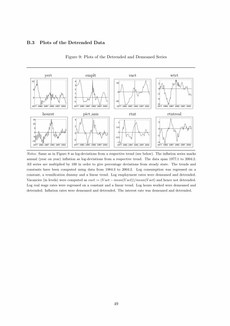
B.3 Plots of the Detrended Data

Figure 9: Plots of the Detrended and Demeaned Series

yert emplt vact wtrt

1977 1982 1987 1992 1997 2002

0

5

10

1977 1982 1987 1992 1997 2002

−1

0

1

2

3

4

1977 1982 1987 1992 1997 2002

−50

0

50

1977 1982 1987 1992 1997 2002−6

−4

−2

0

2

hourst pict ann rtnt rtntreal

1977 1982 1987 1992 1997 2002

−10

−5

0

5

10

15

1977 1982 1987 1992 1997 2002

−2

0

2

4

1977 1982 1987 1992 1997 2002−1

−0.5

0

0.5

1

1977 1982 1987 1992 1997 2002−4

−2

0

2

Notes: Same as in Figure 8 as log-deviations from a respective trend (see below). The inflation series marks

annual (year on year) inflation as log-deviations from a respective trend. The data span 1977:1 to 2004:2.

All series are multiplied by 100 in order to give percentage deviations from steady state. The trends and

constants have been computed using data from 1984:3 to 2004:2. Log consumption was regressed on a

constant, a reunification dummy and a linear trend. Log employment rates were demeaned and detrended.

Vacancies (in levels) were computed as vact := (V act−mean(V act))/mean(V act) and hence not detrended.

Log real wage rates were regressed on a constant and a linear trend. Log hours worked were demeaned and

detrended. Inflation rates were demeaned and detrended. The interest rate was demeaned and detrended.

49

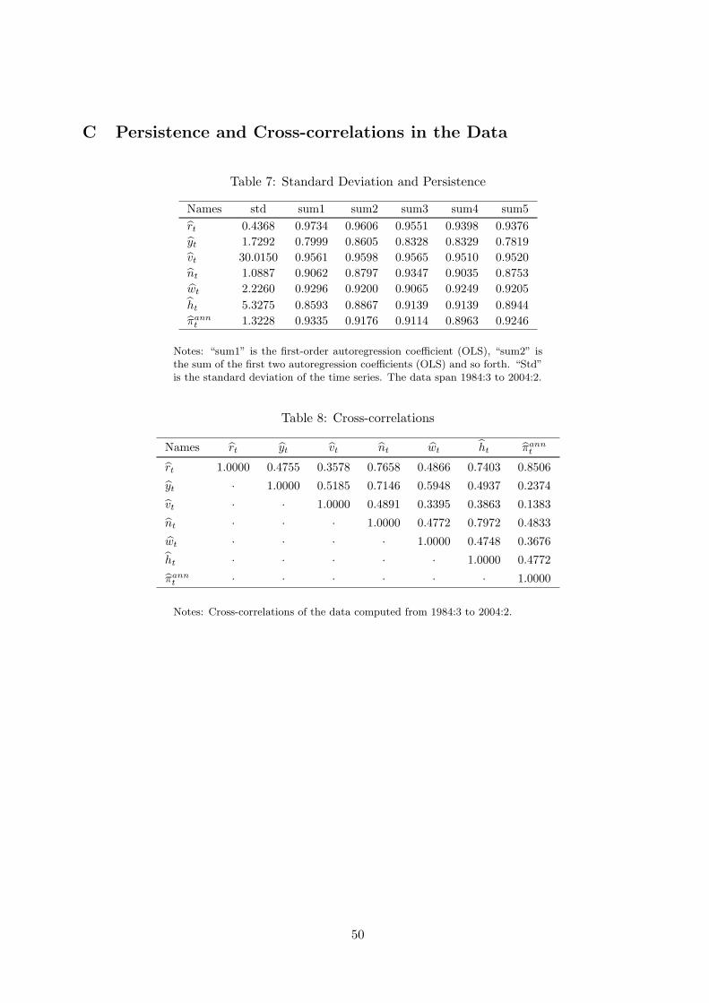
C Persistence and Cross-correlations in the Data

Table 7: Standard Deviation and Persistence

Names std sum1 sum2 sum3 sum4 sum5

rt 0.4368 0.9734 0.9606 0.9551 0.9398 0.9376

yt 1.7292 0.7999 0.8605 0.8328 0.8329 0.7819

vt 30.0150 0.9561 0.9598 0.9565 0.9510 0.9520

nt 1.0887 0.9062 0.8797 0.9347 0.9035 0.8753

wt 2.2260 0.9296 0.9200 0.9065 0.9249 0.9205

ht 5.3275 0.8593 0.8867 0.9139 0.9139 0.8944

πannt 1.3228 0.9335 0.9176 0.9114 0.8963 0.9246

Notes: “sum1” is the first-order autoregression coefficient (OLS), “sum2” isthe sum of the first two autoregression coefficients (OLS) and so forth. “Std”is the standard deviation of the time series. The data span 1984:3 to 2004:2.

Table 8: Cross-correlations

Names rt yt vt nt wt ht πannt

rt 1.0000 0.4755 0.3578 0.7658 0.4866 0.7403 0.8506

yt · 1.0000 0.5185 0.7146 0.5948 0.4937 0.2374

vt · · 1.0000 0.4891 0.3395 0.3863 0.1383

nt · · · 1.0000 0.4772 0.7972 0.4833

wt · · · · 1.0000 0.4748 0.3676

ht · · · · · 1.0000 0.4772

πannt · · · · · · 1.0000

Notes: Cross-correlations of the data computed from 1984:3 to 2004:2.

50

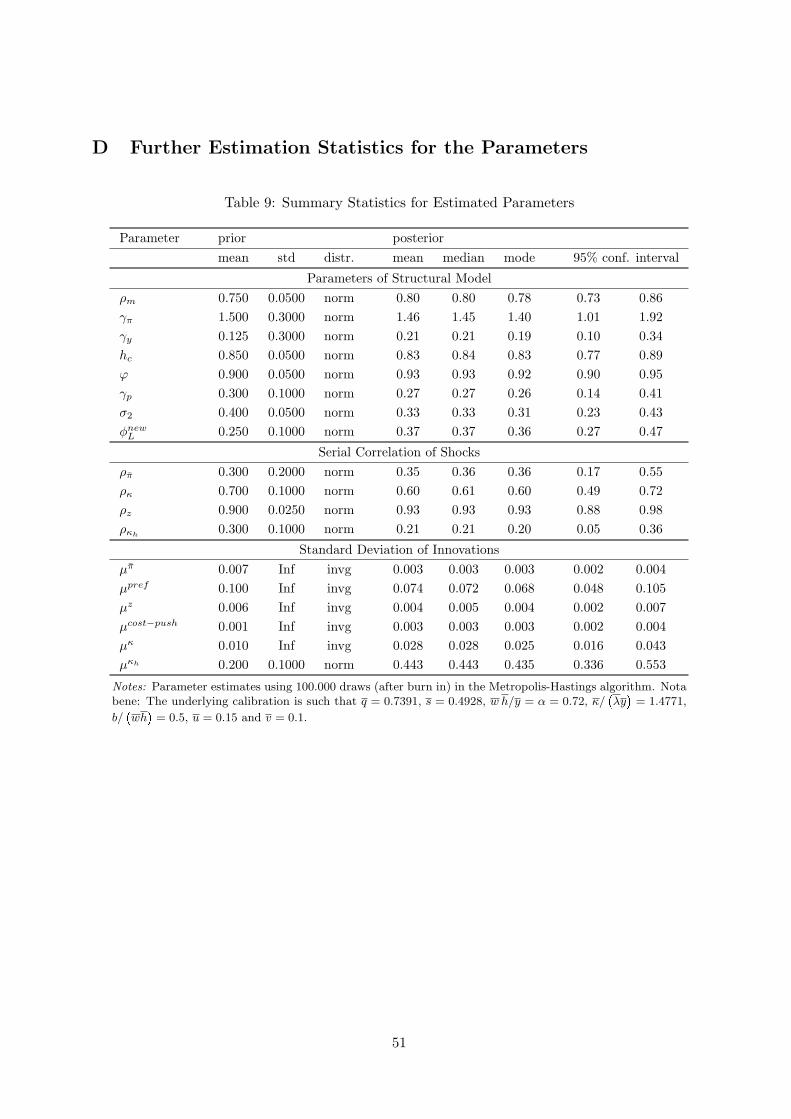
D Further Estimation Statistics for the Parameters

Table 9: Summary Statistics for Estimated Parameters

Parameter prior posterior

mean std distr. mean median mode 95% conf. interval

Parameters of Structural Model

ρm 0.750 0.0500 norm 0.80 0.80 0.78 0.73 0.86

γπ 1.500 0.3000 norm 1.46 1.45 1.40 1.01 1.92

γy 0.125 0.3000 norm 0.21 0.21 0.19 0.10 0.34

hc 0.850 0.0500 norm 0.83 0.84 0.83 0.77 0.89

ϕ 0.900 0.0500 norm 0.93 0.93 0.92 0.90 0.95

γp 0.300 0.1000 norm 0.27 0.27 0.26 0.14 0.41

σ2 0.400 0.0500 norm 0.33 0.33 0.31 0.23 0.43

φnewL 0.250 0.1000 norm 0.37 0.37 0.36 0.27 0.47

Serial Correlation of Shocks

ρπ 0.300 0.2000 norm 0.35 0.36 0.36 0.17 0.55

ρκ 0.700 0.1000 norm 0.60 0.61 0.60 0.49 0.72

ρz 0.900 0.0250 norm 0.93 0.93 0.93 0.88 0.98

ρκh0.300 0.1000 norm 0.21 0.21 0.20 0.05 0.36

Standard Deviation of Innovations

µπ 0.007 Inf invg 0.003 0.003 0.003 0.002 0.004

µpref 0.100 Inf invg 0.074 0.072 0.068 0.048 0.105

µz 0.006 Inf invg 0.004 0.005 0.004 0.002 0.007

µcost−push 0.001 Inf invg 0.003 0.003 0.003 0.002 0.004

µκ 0.010 Inf invg 0.028 0.028 0.025 0.016 0.043

µκh 0.200 0.1000 norm 0.443 0.443 0.435 0.336 0.553

Notes: Parameter estimates using 100.000 draws (after burn in) in the Metropolis-Hastings algorithm. Notabene: The underlying calibration is such that q = 0.7391, s = 0.4928, w h/y = α = 0.72, κ/

�λy

�= 1.4771,

b/�wh

�= 0.5, u = 0.15 and v = 0.1.

51

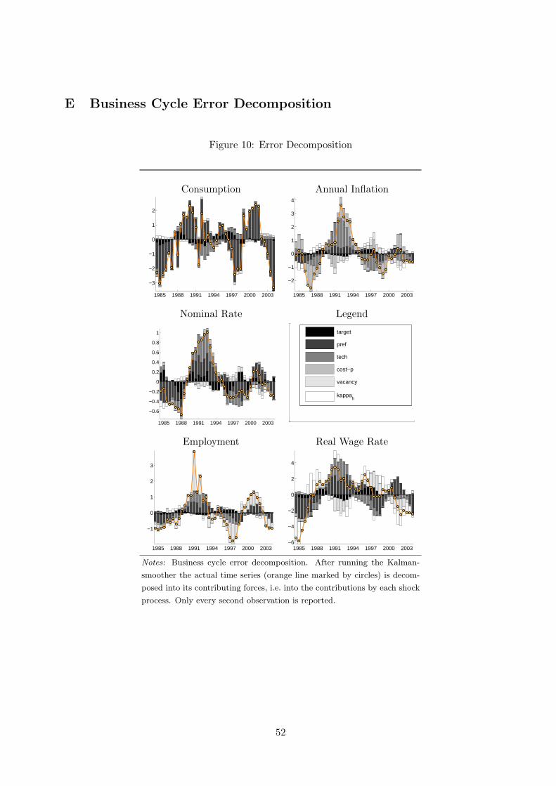
E Business Cycle Error Decomposition

Figure 10: Error Decomposition

Consumption Annual Inflation

1985 1988 1991 1994 1997 2000 2003

−3

−2

−1

0

1

2

1985 1988 1991 1994 1997 2000 2003

−2

−1

0

1

2

3

4

Nominal Rate Legend

1985 1988 1991 1994 1997 2000 2003

−0.6

−0.4

−0.2

0

0.2

0.4

0.6

0.8

1

target

pref

tech

cost−p

vacancy

kappah

Employment Real Wage Rate

1985 1988 1991 1994 1997 2000 2003

−1

0

1

2

3

1985 1988 1991 1994 1997 2000 2003−6

−4

−2

0

2

4

Notes: Business cycle error decomposition. After running the Kalman-

smoother the actual time series (orange line marked by circles) is decom-

posed into its contributing forces, i.e. into the contributions by each shock

process. Only every second observation is reported.

52

F Flexible Labor Market Experiments

The impulse responses (Figures 2 to 7) show the estimated benchmark model along with coun-

terfactual scenarios that are meant to illustrate the behaviour of the economy if the labor market

were more flexible. In detail, they are constructed as follows:

1. A black solid line marks the impulse response when the estimated parameters (at the

posterior mode) are used along with the baseline calibration.

2. A red dotted line marked by triangles shows the impulse responses when the estimated

parameters of the model are used but for eliminating wage rigidity. We set the latter to a

very small value, φnewL = 1.e − 6. This case shows how import the wage rigidity friction is.

Clearly, the steady state relative to the estimated model is not changed by altering φnewL .

3. A green dash-dotted line without markers shows the response when the estimated

parameters of the model are used but the labor market is less rigid in the following sense:

We assume that all workers almost immediately find a job in steady state (not necessarily

outside of steady state) – this means there is an abundance of firms in the market. We set

S ≈ 1 and Q ≈ 0.

• Clearly, this changes the steady state of the model.

• In order to achieve these changes, vacancy posting costs need to be negligible, κ ≈ 0.

σm needs to be adjusted to guarantee well defined probability measures in steady state.

• We maintain the assumption that mrsw = 1 and that h = 1/3. These assumptions are

satisfied by means of a change in κh and b relative to the estimated model.

• This leads to bwh

= 0.1495 instead of 0.5. Note that for each worker, unemployment

becomes less costly (as he is sure to find a job next period), the replacement rate

therefore needs to fall.

• With S ≈ 1, there is full employment prior to production, so U = ρ, which is another

change to the steady state.

4. A blue dashed line without markers is the same as in 3. but that we in addition assume

ρ = 0.07. This implies

• bwh

= 0.0509 instead of 0.5.

5. A green dash-dotted line marked by circles is the same as in 3. but for the fact that we

let only σm (to achieve a well defined probability measure) and κ change, keeping benefits,

b, and κh at the level as in the estimated version.

• This leads to the steady state not being efficient anymore mrsw = 0.9042.

• u = 0.08.

• h = 0.3279.

• bwh

= 0.5080.

53

6. A blue dashed line marked by circles is the same as in 5. but for the fact that we also

assume ρ = 0.07.

• This leads to the steady state not being efficient anymore mrsw = 0.8914.

• u = 0.07.

• h = 0.3272.

• bwh

= 0.5090.

54

G Nominal Wage Adjustment Costs

In this section, we analyze the dynamics of the estimated model when we assume that adjusting

nominal wages causes costs – not the adjustment of the real wage rate. That is, instead of (18)

we let profits be characterized by

ψt(j) := xtyIt (j) − wt(j)ht(j) −

1

2φL

(wt(j)

wt−1(j)

Πt

Π− 1

)2

, (34)

Overall, the behaviour of the economy is very similar to the economy under real wage adjustment

costs and so are the posterior mode parameter estimates. The only difference appears in the

response of the economy to a cost-push shock, which we display for that reason.

55

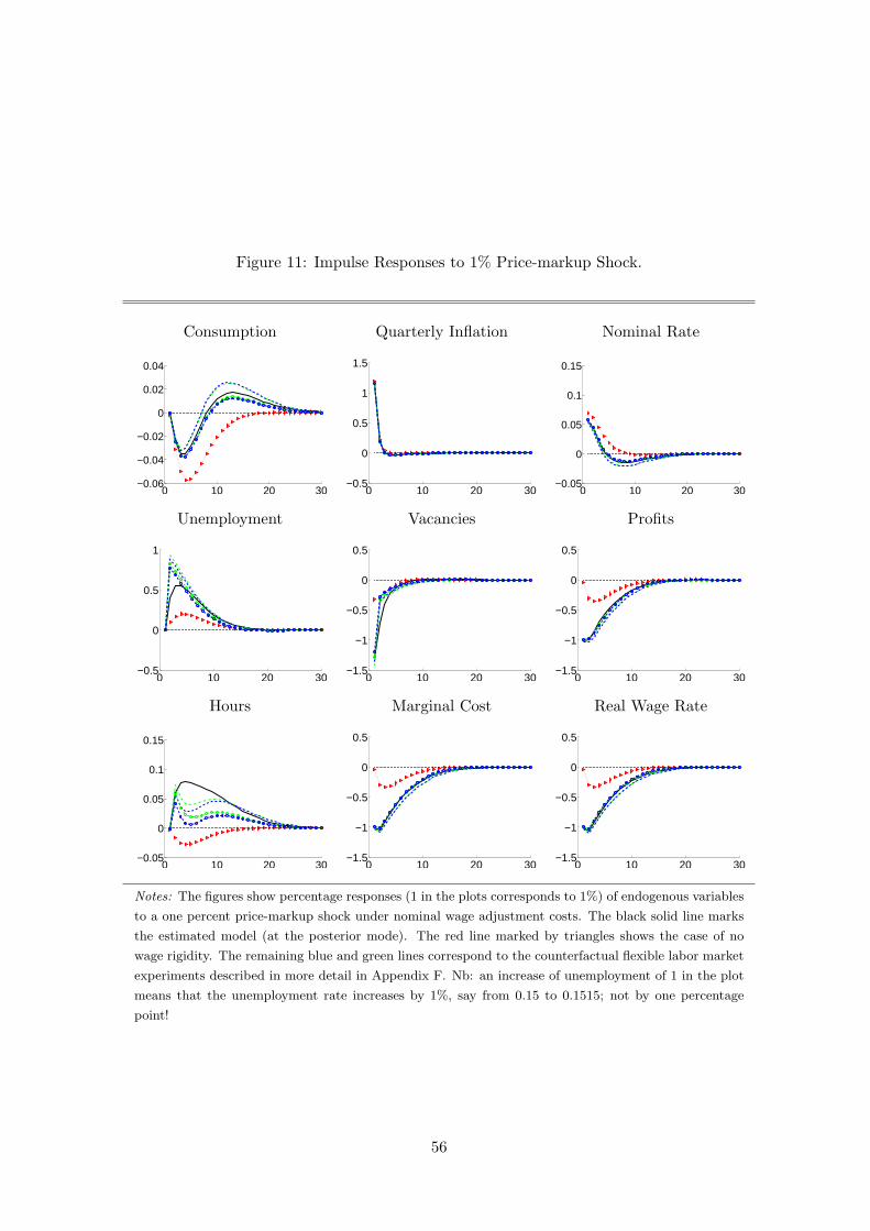
Figure 11: Impulse Responses to 1% Price-markup Shock.

Consumption Quarterly Inflation Nominal Rate

0 10 20 30−0.06

−0.04

−0.02

0

0.02

0.04

0 10 20 30−0.5

0

0.5

1

1.5

0 10 20 30−0.05

0

0.05

0.1

0.15

Unemployment Vacancies Profits

0 10 20 30−0.5

0

0.5

1

0 10 20 30−1.5

−1

−0.5

0

0.5

0 10 20 30−1.5

−1

−0.5

0

0.5

Hours Marginal Cost Real Wage Rate

0 10 20 30−0.05

0

0.05

0.1

0.15

0 10 20 30−1.5

−1

−0.5

0

0.5

0 10 20 30−1.5

−1

−0.5

0

0.5

Notes: The figures show percentage responses (1 in the plots corresponds to 1%) of endogenous variables

to a one percent price-markup shock under nominal wage adjustment costs. The black solid line marks

the estimated model (at the posterior mode). The red line marked by triangles shows the case of no

wage rigidity. The remaining blue and green lines correspond to the counterfactual flexible labor market

experiments described in more detail in Appendix F. Nb: an increase of unemployment of 1 in the plot

means that the unemployment rate increases by 1%, say from 0.15 to 0.1515; not by one percentage

point!

56

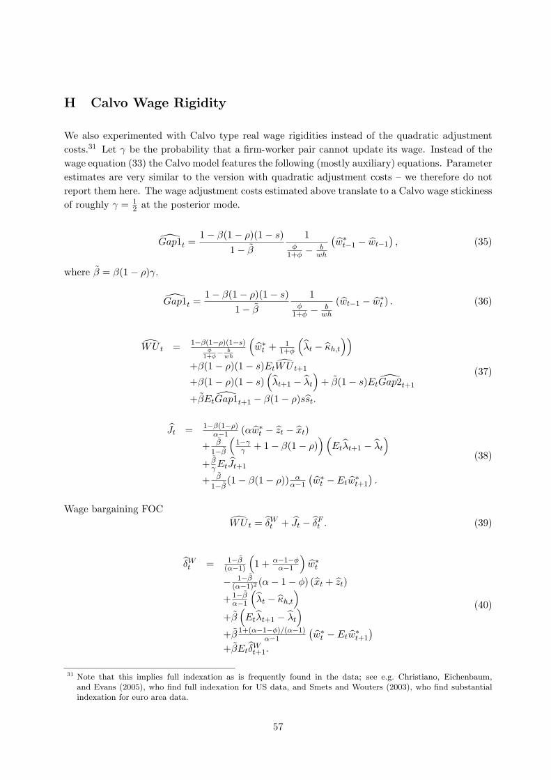
H Calvo Wage Rigidity

We also experimented with Calvo type real wage rigidities instead of the quadratic adjustment

costs.31 Let γ be the probability that a firm-worker pair cannot update its wage. Instead of the

wage equation (33) the Calvo model features the following (mostly auxiliary) equations. Parameter

estimates are very similar to the version with quadratic adjustment costs – we therefore do not

report them here. The wage adjustment costs estimated above translate to a Calvo wage stickiness

of roughly γ = 12 at the posterior mode.

Gap1t =1 − β(1 − ρ)(1 − s)

1 − β

1φ

1+φ − bwh

(w∗

t−1 − wt−1

), (35)

where β = β(1 − ρ)γ.

Gap1t =1 − β(1 − ρ)(1 − s)

1 − β

1φ

1+φ − bwh

(wt−1 − w∗t ) . (36)

WU t = 1−β(1−ρ)(1−s)φ

1+φ− b

wh

(w∗

t + 11+φ

(λt − κh,t

))

+β(1 − ρ)(1 − s)EtWU t+1

+β(1 − ρ)(1 − s)(λt+1 − λt

)+ β(1 − s)EtGap2t+1

+βEtGap1t+1 − β(1 − ρ)sst.

(37)

Jt = 1−β(1−ρ)α−1 (αw∗

t − zt − xt)

+ β

1−β

(1−γ

γ + 1 − β(1 − ρ)) (

Etλt+1 − λt

)

+ βγEtJt+1

+ β

1−β(1 − β(1 − ρ)) α

α−1

(w∗

t − Etw∗t+1

).

(38)

Wage bargaining FOC

WU t = δWt + Jt − δF

t . (39)

δWt = 1−β

(α−1)

(1 + α−1−φ

α−1

)w∗

t

− 1−β(α−1)2

(α− 1 − φ) (xt + zt)

+ 1−βα−1

(λt − κh,t

)

+β(Etλt+1 − λt

)

+β 1+(α−1−φ)/(α−1)α−1

(w∗

t − Etw∗t+1

)

+βEtδWt+1.

(40)

31 Note that this implies full indexation as is frequently found in the data; see e.g. Christiano, Eichenbaum,and Evans (2005), who find full indexation for US data, and Smets and Wouters (2003), who find substantialindexation for euro area data.

57

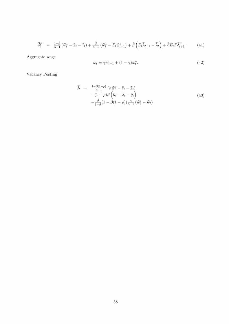
δFt = 1−β

α−1 (w∗t − xt − zt) + β

α−1

(w∗

t − Etw∗t+1

)+ β

(Etλt+1 − λt

)+ βEtF δ

Ft+1. (41)

Aggregate wage

wt = γwt−1 + (1 − γ)w∗t . (42)

Vacancy Posting

Jt = 1−β(1−ρ)α−1 (αw∗

t − zt − xt)

+(1 − ρ)β(κt − λt − qt

)

+ β

1−β(1 − β(1 − ρ)) α

α−1 (w∗t − wt) .

(43)

58