Identifying Similarities, Periodicities and Bursts for ...alumni.cs.ucr.edu/~mvlachos/pubs/sigmod04.pdf · Identifying Similarities, Periodicities and Bursts for Online ... query

Identifying Similarities, Periodicities and Bursts for OnlineSearch Queries

Michail Vlachos †

UC [email protected]

Chris MeekMicrosoft Research

[email protected]

Zografoula VagenaUC Riverside

[email protected]

Dimitrios GunopulosUC Riverside

[email protected]

ABSTRACTWe present several methods for mining knowledge from thequery logs of the MSN search engine. Using the query logs,we build a time series for each query word or phrase (e.g.,‘Thanksgiving’ or ‘Christmas gifts’) where the elements ofthe time series are the number of times that a query is is-sued on a day. All of the methods we describe use sequencesof this form and can be applied to time series data gener-ally. Our primary goal is the discovery of semantically sim-ilar queries and we do so by identifying queries with similardemand patterns. Utilizing the best Fourier coefficients andthe energy of the omitted components, we improve upon thestate-of-the-art in time-series similarity matching. The ex-tracted sequence features are then organized in an efficientmetric tree index structure. We also demonstrate how to ef-ficiently and accurately discover the important periods in atime-series. Finally we propose a simple but effective methodfor identification of bursts (long or short-term). Using theburst information extracted from a sequence, we are able toefficiently perform ’query-by-burst’ on the database of time-series. We conclude the presentation with the description ofa tool that uses the described methods, and serves as an in-teractive exploratory data discovery tool for the MSN querydatabase.

1. INTRODUCTIONOnline search engines have become a cardinal link in the

chain of everyday internet experience. By managing a struc-tured index of web pages, modern search engines have madeinformation acquisition significantly more efficient. Indica-tive measures of their popularity are the number of hits thatthey receive every day. For example, large search servicessuch as Google, Yahoo, and MSN each serve results for tensof millions of queries per day. It is evident that search ser-vices, aside from their information retrieval role, can also

† Part of this work conducted while author was visiting Microsoft Research.

Permission to make digital or hard copies of all or part of this work forpersonal or classroom use is granted without fee provided that copies arenot made or distributed for profit or commercial advantage, and that copiesbear this notice and the full citation on the first page. To copy otherwise, torepublish, to post on servers or to redistribute to lists, requires prior specificpermission and/or a fee.SIGMOD 2004 June 13-18, 2004, Paris, France.Copyright 2004 ACM 1-58113-859-8/04/06 . . . $5.00.

act as a data source for identifying trends, periodicities andimportant events by careful analysis of the queries.

Retaining aggregate query information, such as the num-ber of times each specific query was requested every day, isstorage efficient, can accurately capture descriptive trendsand finally it is privacy preserving. This information couldbe used by the search service to further optimize their in-dexing criteria, or for mining interesting news patterns, thatmanifest as periodicities or peaks in the query log files.

Jan Feb Mar Apr May Jun Jul Aug Sep Oct Nov Dec

Query: cinema

Figure 1: Query demand for the word “cinema” forevery day of 2002

As an illustrative example, let’s consider the query “cin-ema”. In fig. 1 we observe the request pattern for everyday of 2002. We can distinguish 52 peaks that correspondto each weekend of the year. In fact, similar trends can benoticed for specific cinemas as well, indicating a clear prefer-ence of going to the movies during Friday and Saturday. Bydistilling such a knowledge, the engineers of a search servicecan optimize the search of a certain class of queries, dur-ing the days that a higher query load is expected. Such adiscussion is out of the scope of this paper, however possi-ble ways of achieving this could be (for example) enforcinghigher redundancy in their file servers for a specific class ofqueries.

While a significant number of queries exhibit strong weeklyperiodicities, some of them also depict seasonal bursts. Infig. 2 we observe the trend for the word “Easter”, where aclear accumulation of the queries during the relevant months,followed by an immediate drop after Easter. On a similarnote, the query “Elvis” experiences a peak on 16th Aug. ev-ery year (fig. 3), which happens to be the death anniversaryof Elvis Presley.

The above examples are strong indicators about the amountof information that can be extracted by close examinationof the query patterns. To summarize, we believe that pastquery logs can serve 3 major purposes:

1. Recommendations (the system can propose alternative


Query: Easter

Figure 2: Search pattern for the word “easter” dur-ing 2002


Query: Elvis

Figure 3: The demand for query “elvis” for everyday of 2002

or related keywords, that depict similar request pat-terns)

2. Discovery of important news (burst of a specific query)

3. Optimization of the search engine (place similar queriesin same server, since they are bound to be retrieved to-gether)

In the following sections we will explain how one can ex-tract useful information from query logs, in general, and theMSN query logs, in particular.

1.1 ContributionsThis paper makes three main contributions. First we de-

velop new compressed representations for time-series and anindexing scheme for these representations. Because the datawe are dealing with tend to be highly periodic, we describeeach time-series using the k best Fourier coefficients (insteadof the frequently used first ones). In this manner we are ableto provide the tightest yet lower and upper bounds on eu-clidean distance between time-series. We demonstrate howthis representation can be indexed using a variation of ametric tree. The index is very compact in size and exhibitsstrong pruning power due to the bounds that we provide.The new algorithms described in the paper, are presentedin terms of Fourier coefficients but can be generalized to anyorthogonal decomposition with minimal or no effort. Oursecond contribution is an ‘automatic’ method for discover-ing the number of significant periods. Our final contributionis a simple yet effective way to identify bursts in time-seriesdata. We extract burst features that can later be stored ina relational database and subsequently be used to perform‘query-by-burst’ searches, that is, used to find all sequencesthat have a similar pattern of burst behavior.

The paper roadmap is as follows: In Section 2, we describevarious tools for analyzing time-series including the DiscreteFourier Transform (DFT) and the power spectral density.In Sections 3 and 4, we describe our approach to efficientlyrepresenting, storing and indexing a large collection of time-series data. In Section 5, we develop a method for identifyingsignificant periodicities in time-series. In Section 6, we de-scribe a simple but effective approach to burst detection intime-series and its application to ‘query-by-burst’ searching

of a collection of time-series. Finally, in Sections 7 and 8,we experimentally demonstrate the effectiveness of the pro-posed methods and discuss directions for future work.

2. SPECTRAL ANALYSISWe provide a brief introduction to the Fourier decompo-

sition, which we will later use for providing a compressedrepresentation of time-series sequences.

2.1 Discrete Fourier TransformThe normalized Discrete Fourier Transform (DFT) of a

sequence x(n), n = 0, 1 . . . N−1 is a vector of complex num-bers X(f):

X(fk/N ) =1√N

N−1∑n=0

x(n)e−j2πkn/N , k = 0, 1 . . . N − 1

We are dealing with real signals, therefore the coefficientsare symmetric around the middle one. What the Fouriertransform attempts to achieve is, to represent the origi-nal signal as a linear combination of the complex sinusoids

sf (n) = ej2πfn/N√N

. Therefore, the Fourier coefficients repre-

sent the amplitude of each of these sinudoids, after signal xis projected on them.

Time Series

a0

Fourier Components

a1

a2

a3

a4

a5

a6

Figure 4: Decomposition of a signal into the first 7DFT components

2.2 Power Spectral DensityIn order to accurately capture the general shape of a time-

series using a spartan representation, one could reconstructthe signal using just its dominant frequencies. By dominantwe mean the ones that carry most of the signal energy. Apopular way to to identify the power content of each fre-quency is by calculating the power spectral density PSD (orpower spectrum) of a sequence which indicates the signalpower at each frequency in the spectrum. A well known es-timator of the PSD is the periodogram. The periodogramP is a vector comprised of the squared magnitude of theFourier coefficients:

P (fk/N) = ‖X(fk/N )‖2, k = 0, 1 . . . �N − 1

2�

Notice that we can detect frequencies that are at most halfof the maximum signal frequency, due to the Nyquist fun-damental theorem. The k dominant frequencies appear aspeaks in the periodogram (and correspond to the coefficientswith the highest magnitude). From here on, when we referto the best or largest coefficients, we would mean the onesthat have the highest energy and correspond to the tallestpeaks of the periodogram.

3. COMPRESSED REPRESENTATIONS FORPERIODIC DATA

In this section, we describe several compressed representa-tions for periodic data. Our primary goal is to support fastsimilarity searches for periodic data. To that end, we wantour compressed representation to support approximate Eu-clidean distance computations, and, more specifically, goodupper and lower bounds on the actual Euclidean distance be-tween a compressed representation and a query point. Foreach of the representations, we provide algorithms to com-pute upper and lower bounds. Throughout the presentationwe refer to Fourier coefficients because we concentrate onperiodic data, however, our algorithms can be adapted toany class of orthogonal decompositions (such as wavelets,PCA, etc.) with minimal or no adjustments.

3.1 First or Best Coefficients?The majority of the approaches that attempt to speed-up

similarity search are based on the work of Agrawal et al.[1], where the authors lower bound the Euclidean distanceusing the first k Fourier coefficients. The authors use thename GEMINI to describe their generic framework for lowerbounding the distance and utilizing a multidimensional in-dex for candidate retrieval. Rafiei et al. [13] improve on thismethod by exploiting the symmetry of the Fourier coeffi-cients and, thus, provide an even tighter lower bound (usingthe same number of coefficients). We will refer to this lowerbound using the symmetric property as LB-GEMINI.

A later enhancement to this paradigm appears in [14] byWang & Wang. The authors, in addition to the first coef-ficients, also record the error of the approximation to theoriginal sequence. Using this extra information, the authorsprovide a tighter lower bound (LB-Wang) and an upperbound (UB-Wang).

athens 2004

E=72.0

E=65.5

bank

E=120.2

E=48.2

cinema

E=108.0

E=52.8

president

E=92.3

E=45.7

Figure 5: A comparison of using the first coefficientsvs best coefficients in reconstructing the time-seriesfor four queries. Using the best coefficients can sig-nificantly reduce the reconstruction error.

All of the above methods inherently suffer from the as-sumption, that the first coefficients describe adequately thedecomposed signal. While this may be true for some time-series such as random walks, it is not true for many time-series that exhibit strong periodicities. In such sequencesmost of the power is not concentrated in the low frequencycomponents, but is dispersed at various frequencies of thespectrum. Figure 5 depicts the reconstruction error E to theoriginal sequence when using the 5 first Fourier coefficientsagainst the 4 best (the explanation of space requirement foreach method will be deferred until later). It is evident thatusing the coefficients with the most power yields superiorreconstruction even when using fewer components.

The observation that it is best to represent a signal usingthe largest coefficients of a DFT (or other orthogonal de-composition) is not novel. For instance, Wu et al. [15] notethat choosing the best coefficients can be a fast and powerfulalternative to SVD for searching images. It is also useful tonote that in addition to providing a tighter distance approx-imation, the use of the best coefficients, has the advantage ofoffering an immediate overview of the periodic componentsof the data.

3.2 NotationWe will present our algorithms for lower bounding the Eu-

clidean distance, using the best coefficients to approximatea sequence. We begin with some notation first.

We denote a time-series by t = {t1, t2, . . . , tn} and theFourier transformation of t by the capital letter T . Thevector describing the positions of the k largest coefficientsof T is denoted as p+, while the positions of the remainingones as p− (that is p+, p− ⊂ [1, . . . , n]). For any sequence T ,we will store in the database the vector T (p+) or equivalentlyT+. Now if Q is a query in the transformed domain, thenQ(p+) (or Q+) describes a sequence holding the equivalentcoefficients as the vector T (p+). Similarly, Q(p−) ≡ Q− isthe vector holding the analogous elements of T (p−) ≡ T−.

Example: Suppose T = {(1+2i), (2+2i), (1+i), (5+i)} andQ = {(2+2i), (1+i), (3+i), (1+2i)}. The magnitude vectorof T is: abs(T ) = {2.23, 2.82, 1.41, 5.09}. Then, p+ = {2, 4},T (p+) = {(2 + 2i), (5 + i)} and Q(p+) = {(1 + i), (1 + 2i)}.3.3 Algorithm BestMin

In order to speedup similarity search, we compute a lowerbound of the Euclidean distance between the compressedrepresentation T (p+) and the full query dataQ = {Q(p+), Q(p−)}.The squared Euclidean distance is defined as:

D(Q,T )2 = D(Q(p+), T (p+))2 +D(Q(p−), T (p−))2

= ‖Q(p+) − T (p+)‖2 + ‖Q(p−) − T (p−)‖2(1)

The computation of the first part of the distance is trivialsince we have all the required data. For the second partwe are missing the term T (p−), the discarded coefficients.Because we select the best coefficients, we know that themagnitude of each of the coefficients in T (p−) is less than thesmallest magnitude in T (p+). We use minPower = ‖T+

min‖to denote the magnitude of the smallest coefficient in T (p+).

Fact 1. [minProperty] The magnitude of all coefficientsin T (p−) is less than the minimum magnitude of any coeffi-cient in T (p+) (by construction). That is: ‖T+

min‖ ≥ ‖T−i ‖.

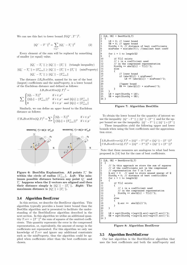
We can use this fact to lower bound D(Q−, T−)2.

‖Q− − T−‖2 =∑

i∈p−‖Q−

i − T−i ‖2 (2)

Every element of the sum will be replaced by somethingof smaller (or equal) value.

‖Q−i − T−

i ‖ ≥ ‖Q−i ‖ − ‖T−

i ‖ (triangle inequality)

‖Q−i − T−

i ‖ + ‖T+min‖ ≥ ‖Q−

i ‖ − ‖T−i ‖ + ‖T−

i ‖ (minProperty)

‖Q−i − T−

i ‖ ≥ ‖Q−i ‖ − ‖T+

min‖The distance LB BestMin, named for its use of the best

(largest) coefficients and the minProperty, is a lower boundof the Euclidean distance and defined as follows:

LB BestMin(Q,T )2 =

∑ ‖Qi − Ti‖2 if i ∈ p+

(‖Qi‖ − ‖T+min‖)2 if i ∈ p− and ‖Qi‖ ≥ ‖T+

min‖0 if i ∈ p− and ‖Qi‖ < ‖T+

min‖Similarly, we can define an upper bound to the Euclidean

distance as follows:

UB BestMin(Q,T )2 =∑ {

‖Qi − Ti‖2 if i ∈ p+

(‖Qi‖ + ‖T+min‖)2 if i ∈ p−

||T min+ ||

||Q i− ||

||Ti−||

MINDIST(Qi−, T

i−) = ||Q

i−|| − ||T

min+ ||

ℑ

ℜ

D(Q i− , T i

− )

||T min+ ||

||Q i− ||

||Ti−||

MAXDIST(Qi−, T

i−) = ||Q

i−|| + ||T

min+ ||

ℑ

ℜ

D(Q i− , T i

− )

Figure 6: BestMin Explanation. All points T−i lie

within the circle of radius ‖T+min‖. Left: The min-

imum possible distance between any point Q−i and

T−i happens when the 2 vectors are aligned and thentheir distance simply is ‖Q−

i ‖ − ‖T−i ‖. Right: The

maximum distance is ‖Q−i ‖ + ‖T−

i ‖.

3.4 Algorithm BestErrorIn this section, we describe the BestError algorithm. This

algorithm typically provides a looser lower bound than theBestMin algorithm and is presented to facilitate the under-standing of the BestMinError algorithm described in thenext section. In this algorithm we utilise an additional quan-tity T.err = ‖T−‖2 the sum of squares of the omitted coeffi-cients. This quantity represents the error in the compressedrepresentation, or, equivalently, the amount of energy in thecoefficients not represented. For this algorithm we only useknowledge of T.err and ignore any additional constraintssuch as the minProperty, thus the algorithm could be ap-plied when coefficients other than the best coefficients arechosen.

1 [LB, UB] = BestMin(Q,T)2 {3 LB = 0; // lower bound4 UB = 0; // upper bound5 DistSq = 0; // distance of best coefficients6 minPower = min(abs(T)); //smallest best coeff78 for i = 1 to length(Q)9 {10 if T[i] exists11 // i is a coefficient used12 // in the compressed representation13 DistSq += abs(Q[i] - T[i])^2;14 else15 {16 // lower bound17 if (abs(Q[i]) > minPower)18 LB += (abs(Q[i]) - minPower)^2;1920 //upper bound21 UB += (abs(Q[i]) + minPower)^2;22 }23 }24 LB = sqrt(DistSq + LB);25 UB = sqrt(DistSq + UB);26 }

Figure 7: Algorithm BestMin

To obtain the lower bound for the quantity of interest weuse the inequality ‖Q−−T−‖ ≥ ‖Q−‖−‖T−‖ and for the up-per bound we use the inequality ‖Q− −T−‖ ≤ ‖Q−‖+ ‖T−‖. These inequalities yield the following upper and lowerbounds when using the best coefficients and the approxima-tion error.

{LB BestError(Q,T )2 = ‖(Q+ − T+)‖2 + (‖Q−‖ − ‖T−‖)2UB BestError(Q,T )2 = ‖(Q+ − T+)‖2 + (‖Q−‖ + ‖T−‖)2

Note that these measures are analogous to what had beenproposed in [14] but for the case of best coefficients.

1 [LB, UB] = BestError(Q,T)2 {3 // In this approach we store the sum of squares4 // of the coefficients not in the compressed5 // representation for T in T.err6 Q.err = 0 // used to store unused energy of Q7 DistSq = 0; // distance of best coefficients8 for i = 1 to length(Q)9 {10 if T[i] exists11 {12 // i is a coefficient used13 // in the compressed representation14 DistSq += abs(Q[i] - T[i])^2;15 }16 else17 {18 Q.err += abs(Q[i])^2;19 }20 }2122 LB = sqrt(DistSq +(sqrt(Q.err)-sqrt(T.err))^2;23 UB = sqrt(DistSq +(sqrt(Q.err)+sqrt(T.err))^2;24 }

Figure 8: Algorithm BestError

3.5 Algorithm BestMinErrorOur last algorithm is the BestMinError algorithm that

uses the best coefficients and both the minProperty and

T.err to obtain a tighter lower bound. The algorithm isdescribed in Figure 9. The algorithm is somewhat morecomplicated than the previous algorithms and we providesome intuitions to aid the reader. The basic idea is to com-pute a lower and an upper bound of this quantity iteratively.For each coefficient not in the compressed representation weconsider two cases:

Case 1: When Q[i] > minPower we use theminProperty. We are certain that we can incrementthe distance by (abs(Q[i]) − minPower)2 for this coef-ficient (line 24). For the lower bound, the most optimisticcase is when this is precisely this distance and “use” pre-cisely minPower energy (line 26). Note that using thismetaphor we would also say that we have used all of theenergy in Q[i]. For the upper bound, the worst case isthat we have use none of the energy from T.err.

Case 2: When Q[i] ≤ minPower the minProperty doesnot apply. In this case we increment the count of unusedenergy from Q by the size of Q[i] (line 30).

Roughly, we compute the lower and upper bound by usingthe upper and lower bound from the BestError case withthe unused energies. More specifically, for the lower bound,we add the distance computed for the known coefficients,the distance computed in case 1 and the best-case distanceusing the overestimate of the unused energy from the missingcoefficients of T . Similarly for the upper bound, we combinethese quantities but use an underestimate of the amount ofenergy used namely T.err.

1 [LB, UB] = BestMinError(Q,T)2 {3 // In this approach we store the sum of squares4 // of the coefficients not in the compressed5 // representation for T in T.err6 LB = 0; // lower bound7 DistSq = 0; // distance of best coefficients8 Q.nused = 0; // energy of unused coeffs for Q9 T.nused = T.err; // energy left for lower bound1011 minPower = min(abs(T)); //smallest best coeff1213 for i = 1 to length(Q)14 {15 if T[i] exists16 // i is a coefficient used17 // in the compressed representation18 DistSq += abs(Q[i] - T[i])^2;19 else20 {21 // lower bound22 if (abs(Q[i]) > minPower)23 {24 LB += (abs(Q[i]) - minPower)^2;25 // at most minPower used26 T.nused -= minPower^2;27 }28 else29 // this energy wasn’t used30 Q.nused += abs(Q[i])^2;31 }32 }3334 // have we used more energy than we had?35 if (T.nused < 0) T.nused = 0;3637 UB=sqrt(DistSq+LB+(sqrt(Q.nused)+sqrt(T.err))^2);38 LB=sqrt(DistSq+LB+(sqrt(Q.nused)-sqrt(T.nused))^2);39 }

Figure 9: Algorithm BestMinError

4. INDEX STRUCTUREAll of the algorithms proposed in section 3, use a different

set of coefficients to approximate each object, thus makingdifficult the use of traditional multidimensional indices suchas the R*-tree [2]. Moreover, in our algorithms we use allthe query coefficients in the new projected orthogonal space,making the adaptation of traditional space partition indicesalmost impossible.

We overcome these challenges by utilizing a metric tree asthe basis of our index structure. Metric trees do not clusterobjects based on the values of the selected features but onrelative object distances. The choice of reference objects,from which all object distances will be calculated, can varyin different approaches. Examples of metric trees includethe Vp-tree [16], M-tree [7] and GNAT [4]. All variationsof such trees, exploit the distances to the reference pointsin conjunction with the triangle inequality to prune partsof the tree, where no closer matches (to the ones alreadydiscovered) can be found.

In this work we will use a customized version of the VP-tree (vantage point tree). The superiority of the VP-treeagainst the R*-tree and the M-tree, in terms of pruningpower and disk accesses, was clearly demonstrated in [5].Here, for simplicity, we describe the modifications in thesearch algorithms for the structure of the traditional staticbinary VP-tree. However all possible extensions to the VP-tree, such as the usage of multiple vantage points [3] or ac-commodation of insertion and deletion procedures [5] canbe implemented on top of the proposed search mechanisms.We provide a brief introduction to the Vp-tree structure,and we direct the interested reader to [6], for a more thor-ough description.

4.1 Vantage Point TreeIn this section, we adapt the notation of [6]. At every

node in a VP-tree there is a vantage point (reference point).The vantage point is used to divide all of the points asso-ciated with that node of the tree into two equal-sized sets.More specifically, the distances of points associated with thevantage point are sorted and the points with distance lessthan the median distance µ are placed in the left subtree(subset S≤), and the remaining ones in the right subtree(subset S>).

To construct a VP-tree for a dataset one simply needs tochoose a method for selecting a vantage point from a setof points and to use this method recursively to construct atree. We use a heuristic method to pick vantage point inconstructing VP-trees. In particular, we choose the pointthat has the highest deviation of distances to the remainingobjects. This can be viewed as an analogue of the largesteigenvector in SVD decomposition.

Suppose that one is searching for the 1-Nearest-Neighbor(1NN) to the query Q and its distance to a vantage pointis DQ,V P . If the best-so-far match is σ we only need to toexamine both subtrees if µ − σ < DQ,V P < µ + σ. In anyother case we only have to examine one of the subtrees.

Typically VP-trees are built using the original data, thatis, the vantage points are not compressed representations.In our approach, we adapt the VP-tree to work with a com-pressed representation. By doing so we significantly reducethe amount of space needed for the index. Of course, thedownside of using a compressed representation as the van-tage points is that the distance computation is no longer

VP

S≤

S>

µ

σUB

VP2σ

VP

(a) (b) (c)

LB

UB

σUB

Figure 10: (a) Separation into two subsets accordingto median distance, (b) Pruning in VP-tree usingexact distances, (c) Pruning in VP-tree using upperand lower bounds

exact and we must resort to using bounds. Our approach isto construct the VP-tree using an uncompressed represen-tation and, then, after it is constructed, convert the vantagepoints to the appropriate compressed representation and IDof the original object (time series). By doing so, we obtainexact distances during the construction process. One canoptimize this process slightly by compressing a point imme-diately after it is selected to be a vantage point.

We will modify the knn search algorithm to utilize thelower and upper bounds of the uncompressed query Q toa compressed object (whether this is vantage point or leafobject). So, suppose for the best-so-far match we have alower bound σLB and a upper bound σUB . We will onlyvisit the left subtree if the upper bound distance between Qand the current vantage point V P is: UBQ,V P < µ− σUB .This happens since for any R ∈ S> the distance between Rand Q is:

D(Q,R) ≥ |D(R, V P ) −D(Q,V P )| (triangle inequality)

≥ |µ−D(Q,V P )| (by construction)

≥ |µ− UB(Q,V P )|> |µ− (µ− σUB)| (assumption)

= σUB

and since our best match is less than σUB this part of thetree can be safely discarded. In a similar way we will onlytraverse the right subtree (S>) if the lower bound betweenQ and V P is: LBQ,V P > µ+ σUB. For any other case bothsubtrees will have to be visited (fig. 10 (c))

The index scan is performed using a depth-first traversal,and σLB , σUB are updated both by compressed objects inthe leaves as well as by the vantage points. Additionally, asan optimization, the search is heuristically ‘guided’ towardsthe most promising nodes. Our heuristic works as follows:Consider the annulus (disc with a smaller disc removed) de-fined by the upper and lower bounds for a query centeredaround the current vantage point. We can divide this areainto two areas (one of them possibly empty); one region inwhich the points that are further away than the median µfrom the current vantage point and one in which the pointsare closer than the median. Each child of the current van-tage point is naturally associated with one of these regionsand we choose the child node associated with the region oflarger size. Suppose, for example, that the lower and up-per bounds of the query with respect to the current vantagepoint are in the range [LB-UB], as shown by the gray linein fig. 10(c). Because the distance range overlaps more with

the subset S≤, we should follow this subset first. It seemslikely that this approach will find a good match sooner andleading to quicker pruning of other parts of the tree.

Even though we prune parts of the tree using the upperbound σUB of the best-so-far match (and not the exact dis-tance) the pruning power of the index is kept very high,because the use of algorithm BestMinError can providea significantly tight upper bound. This will be explicitlydemonstrated in the experimental section.

After the tree traversal we have a set of compressed ob-jects with their lower and upper bounds. The smallest upperbound (SUB) is computed and all objects with lower boundhigher than SUB are excluded from examination. The fullrepresentation of the remaining objects is retrieved from thedisk, in the order suggested by their lower bounds. A simpleversion of the 1NN search (without the traversal to the mostpromising node) is provided in fig. 11.

5. DETECTING IMPORTANT PERIODSUsing the periodogram we can visually identify the peaks

as the k most dominant periods (period =1/frequency). How-ever, we would like to have an automatic method that willreturn the important periods for a set of sequences (e.g.,for the knn results). What we need is to set an appropri-ate threshold in the power spectrum, that will accuratelydistinguish the dominant periods. We will additionally re-quire that this method not only identifies the strong periods,but also reduces the number of false alarms (i.e., it doesn’tclassify unimportant periods as important).

5.1 Number of significant periodsNext we devise a test to separate the important periods

from the unimportant ones. To do so one needs to specifyexactly what is meant by a non-periodic time series. Ourcanonical model of a non-periodic time-series is a sequenceof points that are drawn independently and identically froma Gaussian distribution. Clearly this type of sequence canhave no meaningful periodicities. In addition, under this as-sumption, the magnitudes of the coefficients of the DFT aredistributed according to an exponential distribution. Evenwhen the assumption of i.i.d. Gaussian samples does nothold, it is often the case that the histogram of the coefficientmagnitudes has an exponential shape. Fig. 12 illustratesthis for several non-periodic time series. Our approach is toidentify significant periods by identifying outliers accordingto an exponential distribution.

Starting from the probability distribution function of theexponential distribution, we derive the cumulative distribu-tion function:

f(x) = λe−λx ⇒P (x ≥ A) = 1 −

∫ ∞

0

f(x)dx = e−λx

where λ is the inverse of the average value. The importantperiods will have powers that deviate from the power con-tent of the majority of the periods, therefore we will seekfor infrequent powers. Consequently, we will set this proba-bility p to a very low value and calculate the derived powerthreshold. For example, if we want to be confident withprobability 99.99% that the returned periods will be sig-nificant we have: (100 − 99.99)% = 0.01% = 0.0001, and

NNSearch(Q){Input: Uncompressed Query QOutput: Nearest Neighbor

S <- Search(root-of-index, Q)// S = set of compressed objects returned from// tree traversal with associated// lower (S.LB) and upper bounds (S.UB)

SUB = min(S(i).UB); // smallest upper boundDelete({S(i) | S(i).LB> SUB}); // prune objectsSort(S(i).LB); // sort by lower bounds

bestSoFar.dist = inf;

for i=1 to S.Length{

if S(i).LB > bestSoFar.distreturn bestSofar

retrieve uncompressed time-series Tof S(i) from database

dist = D(T,Q); // full euclidean

if dist < bestSoFar{

bestSoFar.dist = dist;bestSoFar.ID = T;

}}

}

Search(node,Q){Input: Node of Vp-tree, uncompressed query QOutput: set of unpruned compressed objects withassociated lower and upper bounds

if node is leaf{

for each compressed time-series cT in node{

(LB,UB) <- BestMinError(cT,Q);queue.push(cT,LB,UB); // sorted by UB

}}else // vantage point{

(LB,UB) <- BestMinError(VP,Q);queue.push(VP,LB,UB);sigmaUB = queue.top; // get best upper bound

if UB < node.median - sigmaUBsearch(node.left,Q);

if LB > node.median + sigmaUBsearch(node.right,Q);

}}

Figure 11: 1NN Search for VP-tree with compressedobjects

the power probability is set to 10−4. Solving for the powerthreshold Tp we get:

ln(p) = ln(e−λTp) = −λTp ⇒

Tp = − ln(p)

λ= −µ · ln(p)

and µ is the average signal power. For example for con-fidence 99.99%, p = 10−4 and if the average signal power0.02 (= 1/n

∑i x

2i ), then the power density threshold value

is Tp = 0.0184.

Examples: We demonstrate the accuracy and usefulness

Sequence 1 PSD histogram 1



Figure 12: Typical histogram of power spectrum forvarious non-periodic sequences follow an exponen-tial distribution

of the proposed method with several examples. In fig. 13we juxtapose the demand of various queries during 2002with the periods identified as important. We can distin-guish a strong weekly component for queries ‘cinema’ &‘nordstrom’, while for ‘full moon’ the monthly periodicityis accurately captured. For the last example we used a se-quence without any clear periodicity and again our methodis robust enough to set the threshold high enough, thereforeavoiding false alarms. The large peak in the data happensduring the day the famous British actor died, and of courseits identification is important for the discovery of important(rare) events. We will expound how to discover such (ormore subtle) bursts in the following section.

Query *cinema*

0 0.1 0.2 0.3 0.4 0.50

0.1

0.2

Pow

er D

ensi

ty

frequency

0.0411

P1= 7

P2= 3.5

P3= 91

Query *full moon*

0 0.1 0.2 0.3 0.4 0.50

0.1

0.2

Pow

er D

ensi

ty

frequency

0.047

P1= 30.33P2= 7

P3= 14.56

Query *nordstrom*

0 0.1 0.2 0.3 0.4 0.50

0.2

0.4

Pow

er D

ensi

ty

frequency

0.0379

P1= 7

P2= 3.5P3= 121.33

Query *dudley moore*

0 0.1 0.2 0.3 0.4 0.50

0.05

0.1

Pow

er D

ensi

ty

frequency

0.05

Figure 13: Discovered periods for four queries usingthe power density threshold

6. BURST DISCOVERY

Our final method for knowledge extraction, involves thedetection of bursts. In the setting of this work, interactiveburst discovery will involve three tasks; first we have to de-tect the bursts, then we need to compact them, in order tofacilitate an efficient storage scheme in a DBMS system andfinally based on compacted features we can pose queries inthe system (‘query-by-burst’). The query-by-burst featurecan be thought of as a fast alternative of weighted Euclideanmatching, where the focus is given on the bursty portionof a sequence. Compared to the work of Zhu & Shasha[17], our approach is more flexible since it does not requirea custom index structure, but can easily be integrated inany relational database. Moreover, our framework requiressignificantly less storage space and in addition we can sup-port similarity search based on the discovered bursts. Ourmethod is also simpler and less computationally intensivethan the work of [11], where the focus is on the modeling oftext streams.

6.1 Burst DetectionFor discovering regions of burst in a sequence, our ap-

proach is based on the computation of the moving aver-age (MA), with a subsequent annotation of bursts as thepoints with value higher than x standard deviations abovethe mean value of the MA. More concretely:

1. Calculate Moving Average MAw of length w

for sequence t = (t1, ...tn).2. Set cutoff = mean(MAw) + x*std(MAw)

3. Bursts = {ti| MAw(i) > cutoff }For our database we used sliding windows of two lengthsw; one used a moving average of 30 days (long-term bursts)and one a 7 day moving average (short-term bursts), whichwe found to cover sufficiently well the bursts ranges in thedatabase sequences. Typical values for the cutoff point are1.5-2 times the standard deviation of the MA. In fig. 14,we can see a run of the above algorithm on the query ‘Hal-loween’ during the year 2002. We observe that the burst dis-covered is indeed during the October and November months.In fig. 15 another execution of the algorithm is demon-strated, this time for the word “Easter”, during a span ofthree years.


Halloween

DataMoving AverageCutoff


DataBurst

Figure 14: User demand for the query ‘Halloween’during 2002 and the bursts discovered

6.2 Burst CompactionWe would like to identify in an large database, sets of

sequences that exhibit similar burst patterns. In order to

2000 2001 2002

Easter 2000−2002

DataMoving AverageCutoff

2000 2001 2002

DataBurst

Figure 15: History of the query ‘Easter’ during theyears 2000-2002 and the bursts discovered

speedup this process, we choose not to store all points ofthe bursty portion of a sequence, but we will perform somekind of feature compaction.

For this purpose, we represent each consecutive sequenceof values identified as a burst, by their average value. Sup-pose, for example, that B(X) = (xp, . . . , xp+k, xq, . . . , xq+m)signify the points identified as bursts on a sequence X =(x1, x2, . . . , xn). In this case, sequence B contains two burstregions and the compact form of the burst is:

B(X) = (︷︸︸︷xp, xp+1 . . . xp+k,

︷︸︸︷xq, xq+1 . . . xq+m)

= (B(X)1 , B

(X)2 )

= ([p, p+ k,1

p+ k − 1

p+k∑i=p

xi], [q, q +m,1

q +m− 1

q+m∑i=q

xi])

In other words, each burst is characterized by a triplet [start-Date, endDate, average value], indicating the start and end-ing point of the burst, and the average burst value duringthat period, respectively. The length of a burst B will beindicated by |B| = endDate− startDate+ 1.

The burst triplets of each sequence can now be stored asrecords in a DBMS table with the following fields:

[sequenceID, startDate, endDate, average burst

value]

In fig. 16 we elucidate the compact burst representation,as well as the high interpretability of the results. For thequery ‘flowers’, we discover two long-term bursts during themonths February and May. This is consistent with our ex-pectation that flower demand tends to peak during Valen-tine’s Day and Mother’s Day. For the query ‘full moon’(using short term burst detection) we can effectively distuin-guish the monthly bursts (that is once for every completionof the moon circle).

6.3 Burst Similarity MeasuresNow we will define the similarity Bsim between the burst

triplets. Let time-series X and Y and their respective set of

burst features B(X) = (B(X)1 , . . . , B

(X)k ) and

B(Y ) = (B(Y )1 , . . . , B

(Y )m ). We have :

BSim =k∑

i=1

m∑j=1

intersect(B(X)i , B

(Y )j ) ∗ similarity(B

(X)i , B

(Y )j )


Query *flowers*


Query *Full Moon*

Discovered Bursts

Figure 16: Compact burst representation by us-ing the average value of the bursts, and high in-terpretability of the discovered bursts.

where similarity captures how close the average burst val-ues are:

similarity(B(X)i , B

(Y )j ) =

1

1 + dist(B(X)i , B

(Y )j )

=1

1 + (avgV alue(B(X)i ) − avgV alue(B

(Y )j )

and intersect returns the degree of overlap between thebursts:

intersect =1

2(overlap(B

(X)i , B

(Y )j )

|B(X)i |

+overlap(B

(X)i , B

(Y )j )

|B(Y )j |

)

The function overlap simply calculates the time intersec-tion between two bursts. fig. 17 briefly demonstrates forbursts A,B the calculation of overlap(A,B).

0

2000

4000

6000

Fully overlapping Bursts Partially overlapping Bursts No overlap between Bursts

A

BA A

B B

overlap(A,B) overlap(A,B)

dist(A,B)

overlap(A,B) = 0

Figure 17: Burst overlaps between time-series

Before the burst features are extracted, the data are stan-dardized (subtract mean, divide by std) in order to compen-sate for the variation of counts for different queries.

Execution in a DBMS system: Since all identified burstfeatures are stored in a database system, it is very efficient todiscover burst features that overlap with the query’s bursts.

In fig. 18 we illustrate the search for overlapping bursts.Essentially we need to discover features with startDate ear-lier than the ending date of the query burst and with endDatelater than the burst starting date. This procedure is ex-tremely efficient, if we create an index (basically a B-tree)on the startDate and endDate attributes. For the qualify-ing burst features, the similarity measures are accordinglycalculated for their respective sequences as described.

startDateendDate

QueryBurst Q

SELECT Burst B FROM DatabaseWHERE B.startDate<Q.endDate

ANDB.endDate>Q.startDate

Database

Bursts B

Figure 18: Identifying Overlapping Bursts in aDBMS

In fig. 19 we show some results of burst similarity mea-sure. It is prevalent that ‘query-by-burst’ can be a powerfulasset for our knowledge discovery toolbox. This type of rep-resentation and approach to search is especially useful forfinding matches for time series with non-periodic bursts.

7. EXPERIMENTAL EVALUATIONNow we will demonstrate with extensive experiments the

effectiveness of the new similarity measures and comparetheir performance with other widely used Euclidean approx-imations. We also exhibit that our bounds lead to goodpruning performance and that our approach to indexing hasgood performance on nearest neighbor queries.

For our experiments all sequences had length of 1024 points,capturing almost 3 years of query logs (2000-2002). Thedataset sizes range up to 215 time-series, effectively con-taining more than 30 million daily measurements in ourdatabase. All sequences were standardized and the querieswere sequences not found in the database. The experimentshave been conducted on a 2Ghz Intel Pentium 4, with 1GBof RAM and 60GB of secondary storage.

7.1 Space RequirementsFor fair comparison of all competing methods, it is imper-

ative to judge their performance when the same amount ofmemory is alloted for the coefficients of each approach.

The storage of the first k Fourier coefficients requires just2k doubles (or 2k*8 bytes). However, when utilizing thek best coefficients for each sequence, we also need to storetheir positions in the original DFT vector. That is, thecompressed representation with the k largest coefficients isstored as pairs of [position-coefficient].

For the purposes of our experiments 2048 points are morethan adequate, since they capture more than 5 years of logdata for each query. Taking under account the symmetricproperty we just need to store 1024 positions, so 10 bitswould be sufficient. However, since on disk we can writeonly as multiples of bytes, each position requires 2 bytes. Inother words, each coefficient in our functions requires 16+2bytes, and if GEMINI uses k coefficients, then our methodwill use �16k/18� = �k/1.125� coefficients.

For some distance measures we also use one additionaldouble to record the error (sum of squares of the remain-ing coefficients). Therefore, for the measures that don’t usethe error we need to allocate one additional number and wechoose this to be the middle coefficient of the full DFT vec-tor, which is a real number [12] (since we have real data withlengths power of two). If in some cases the middle coefficienthappens to be one of the k best ones, then these sequencesjust use 1 less double than all other approaches. The follow-

2000 2001 2002

query = world trade center

pentagon attack

nostradamus prediction

2000 2001 2002

query = hurricane

www.nhc.noaa.gov

tropical storm

2000 2001 2002

query = christmas

gingerbread men

rudolph the red nosed reindeer

Figure 19: Three examples of ‘query-by-burst’. We depict a variety of interesting results discovered whenusing the burst similarity measures.

ing table summarizes how the same amount of memory isallocated for each compressed sequence of every approach.

GEMINI c First Coeffs + Middle CoeffWang c First Coeffs + ErrorBestMin �c/1.125� Best Coeffs + Middle CoeffBestError �c/1.125� Best Coeffs + ErrorBestMinError �c/1.125� Best Coeffs + Error

Table 1: Requirements for usage of same storage foreach approach

Therefore, when in the following figures we mention mem-ory usage of [2*(32)+1] doubles, the number in parenthesisessentially denotes the coefficients used for the GEMINI andWang approach (+ 1 for the middle coefficient or the error,respectively). For the same example, our approach uses the28 best coefficients but has the same memory requirements.

7.2 Tightness of BoundsThis first experiment measures the tightness of the lower

and upper bounds of our algorithms. We compare with theapproaches that utilize the first coefficients (GEMINI) andwith the bounds proposed by Wang using the first coeffi-cients in conjunction with the error.

In figures 20 and 21 we show the lower and upper boundsfor all approaches in conjunction with the actual Euclideandistance. The distance shown is the cumulative euclideandistance over 100 random pairwise distance computationsfrom the MSN query database. First, observe that theBestMinError provides the best improvement. Second, theWang approach provides the best approximation when thefirst coefficients are used. Using BestMinError there is anoticeable 6-9% improvement in the lower bound and a 13-18% improvement in the upper bounds, compared to thenext best method (LB Wang). However, as we will see inthe following section, this improvement in distance leads

0 2000 4000

Full Euclidean

LB_GEMINI

LB_Wang

LB_BestError

LB_BestMin

LB_BestMinError

Cumulative Distance

Memory = 2*(8)+1 doublesImprovement = 6.1533%

3770

1914

2017

1961

2042

2141

2000 4000Cumulative Distance

Memory = 2*(16)+1 doublesImprovement = 7.9435%

3770

2167

2291

2293

2366

2473


NumCoeffs = 2*(32)+1 doublesImprovement = 9.7063%

3770

2403

2546

2636

2674

2793

Figure 20: Lower Bounds: The methods taking ad-vantage of the best coefficients (and especially Best-MinError) outperform the approaches using the firstcoefficients.

0 5000 10000

Full Euclidean

UB_GEMINI

UB_Wang

UB_BestError

UB_BestMin

UB_BestMinError

Cumulative Distance

Memory = 2*(8)+1 doubles Improvement = 13.355%

3770

5676

5325

9081

4918

N/A



3770

5512

5077

6632

4665

N/A



3770

5366

4835

5399

4400

N/A

Figure 21: In the calculation of Upper Bounds, Best-MinError provides the tightest Euclidean approxi-mation

to a significant improvement in pruning power. For theremainder of the paper we do not report results for theBestMin and BestError methods due to the superiorityof the BestMinError method.

7.3 Pruning PowerWe evaluate the effectiveness the Euclidean distance bounds

in a way that is not effected by implementation details orthe use of an index structure. The basic idea is to measure

the average fraction F of the database objects examined inorder to find the 1NN for a set of queries. In order tocompute F for a given query Q, we first compute the lowerand upper bound distances to Q for each object using itscompressed representation. Note that we do not computean upper bound for GEMINI. We find the smallest upperbound (SUB) and objects that have LowerBound > SUBare pruned. For the remaining sequences the full representa-tions are retrieved from disk and compared with the query,in increasing order as suggested by the lower bounds. Westop examining objects, when the current lower bound ishigher than the best-so-far match. Similar methods for eval-uation have also appeared in [8, 10].

The results we present are for a set of 100 randomly se-lected queries not already in the database. Fig. 22 showsthe dramatic reduction in the number of objects that needto be examined, a reduction that ranges from 10-35% com-pared to the next best method. These positive effects canbe attributed to four reasons:

• Our methods make use of all coefficients of a query,thus giving tigher distance estimates.

• The best coefficients provide a high quality reconstruc-tion of the indexed sequences.

• The knowledge of the remaining energy significantlytightens the distance estimation.

• Finally, the calculation of upper bounds, reduces thenumber of candidate sequences that need to be exam-ined.

2*(32)+12*(16)+1

2*(8)+1

0

0.1

0.2

0.3

0.4

0.5

0.6

Dataset Size

GEMINIWangBestMinError

−8.3

−17

−33.6

−9.7

−19.2

−35.3

−11

−21.4

−35.6

Doubles per S

equenc8192

16384

32768

Figure 22: Fraction of database objects examinedfor three compression factors. BestMinError in-spects the least number of objects, even thoughfewer coefficients are used.

7.4 Index PerformanceIn our final experiment, we measure the CPU time re-

quired by the Linear Scan and our index structure to returnthe 1-Nearest-Neighbor to 50 queries (not already found inthe database).

For our test datasets, due to the high compression, theindex size and the compressed features could easily fit inmemory, therefore we provide two running times for our in-dex; the first one is with all the compressed features in mem-ory and the second one is with the compressed sequences insecondary storage.

In fig. 23 we report the running time for the linear scanwhich uses the uncompressed sequences, in comparison withthe index running time for various compression factors anddatabase sizes. Both approaches were optimized to performan early termination of the Euclidean distance, when therunning sum exceeded the best-so-far match. We can ob-serve that when the compressed features are retrieved fromthe disk the index is approximately 20-25 times faster thanthe sequential scan. In the case where the compressed se-quences fit in memory the speedup exceeds the 120 times.Notice that this running time, includes the random I/Oto read the uncompressed sequences from the disk. Thebest performance for the memory resident index in observedwhen more coefficients are utilized. However, for the exter-nal memory index the highest compression factors achievethe best performance. This is attributed to the reduced I/Ocosts for this case, and it is also a significant indicator thata few number of the best coefficients can capture accuratelythe sequence shape. The result is very promising since itdemonstrates that we can achieve exceptional performancewith compact external memory indices.

2*(8)+12*(16)+1

2*(32)+132768

16384

8192

0

500

1000

1500

2000

2500

Doubles per s

equence

Database Size

Run

ning

Tim

e (s

ec)

Linear ScanIndex on DiskIndex in Memory

Figure 23: Fraction of running time required by ourindex structure to return the 1NN, compared toLinear Scan. The observed speedup is at least 20times (for disk based index), exceeding 2 orders ofmagnitude when the compressed features reside inmemory.

7.5 The S2 Similarity ToolWe conclude this section with a brief description of a tool

that we developed which incorporates many of the featuresdiscussed in this paper.

Our tool is called S2 which stands for Similarity Tool. Theprogram is implemented in C# and it interacts with a re-mote SQL database server to retrieve the actual sequences,while the compressed features are stored locally for faster ac-cess. Realtime response rates are observed for the subset ofthe top 80000+ sequences, whose compressed representationthe program utilizes. The user can pose a search keywordand similar sequences from the MSN query database are re-trieved. A snapshot of the main window form is presentedin fig. 24. The program offers three major functionalities:

• Identification of important periods

• Similarity search

• Burst Detection & Query-by-Burst

The user can examine at any time the quality of the time-series approximation, based on the best-k coefficients. Ad-ditionally, a presentation of the discovered bursts for thesequence is also possible. It is at the user’s discretion to useall or some of the best-k periods for similarity search, there-fore effectively concentrating on just the periods of interest.Similar functionality is provided for burst search.

Figure 24: Snapshot of the S2 tool and demonstra-tion of ’query-by-burst’

8. CONCLUSIONS AND FUTURE WORKIn this work we proposed methods for improving the tight-

ness of lower and upper bounds on Euclidean distance, bycarefully selecting the information retained in the compressedrepresentation of sequences. In addition, the selected infor-mation allows us to utilize a full query rather than a com-pressed representation of the query which further improvesthe bounds and significantly improves the index pruning per-formance. Moreover, we have presented simple and effectiveways for identifying periodicities and bursts. We appliedthese methods on real datasets from the MSN query logsand demonstrated with extensive examples the applicabilityof our contributions.

In the approach described here, we choose a fixed numberof coefficients for each object. A natural extension of thisapproach is to allow for a variable number of coefficients.For instance, one possibility in the case of Fourier coeffi-cients is to add the best coefficients until the compressedrepresentation contains k% of the energy in the signal (or,equivalently, the error is below some threshold). This typeof compressed representation is easily indexed using our cus-tomized VP-tree index.

In addition, we feel that this approach can be fruitfullyapplied for other types of similarity queries. In particular,we believe that a similar approach could prove useful in thecomputation of linear-cost lower and upper bounds for ex-pensive distance measures like dynamic time warping [9].

9. REFERENCES[1] R. Agrawal, C. Faloutsos, and A. Swami. Efficient

Similarity Search in Sequence Databases. In Proc. ofthe 4th FODO, pages 69–84, Oct. 1993.

[2] N. Beckmann, H.-P. Kriegel, R. Schneider, andB. Seeger. The r*-tree: An efficient and robust accessmethod for points and rectangles. In Proc. of ACMSIGMOD, 1990.

[3] T. Bozkaya and M. Ozsoyoglu. Distance-basedindexing for high-dimensional metric spaces. In Proc.of SIGMOD, 1997.

[4] S. Brin. Near neighbor search in large metric spaces.In Proc. of 21th VLDB, 1995.

[5] A. W. chee Fu, P. M. Chan, Y.-L. Cheung, andY. Moon. Dynamic vp-tree indexing for n-nearestneighbor search given pair-wise distances. Journal ofVLDB, 2000.

[6] T. Chiueh. Content based image indexing. In Proc. ofVLDB, 1994.

[7] P. Ciaccia, M. Patella, and P. Zezula. M-tree: Anefficient access method for similarity search in metricspaces. In Proc. of 23rd VLDB, pages 426–435, 1997.

[8] J. Hellerstein, C. Papadimitriou, and E. Koutsoupias.Towards an analysis of indexing schemes. In Proc. of16th ACM PODS, 1997.

[9] E. Keogh. Exact indexing of dynamic time warping. InProc. of VLDB, 2002.

[10] E. Keogh, K. Chakrabarti, S. Mehrotra, andM. Pazzani. Locally adaptive dimensionality reductionfor indexing large time series databases. In Proc. ofACM SIGMOD, pages 151–162, 2001.

[11] J. Kleinberg. Bursty and hierarchical structure instreams. In Proc. of 8th SIGKDD, 2002.

[12] A. Oppenheim, A. Willsky, and S. Nawab. Signals andSystems, 2nd Edition. Prentice Hall, 1997.

[13] D. Rafiei and A. Mendelzon. Efficient retrieval ofsimilar time sequences using dft. In Proc. of FODO,1998.

[14] C. Wang and X. S. Wang. Multilevel filtering for highdimensional nearest neighbor search. In ACMSIGMOD Workshop on Research Issues in DataMining and Knowledge Discovery, 2000.

[15] D. Wu, D. Agrawal, A. E. Abbadi, A. K. Singh, andT. R. Smith. Efficient retrieval for browsing largeimage databases. In Proc. of CIKM, pages 11–18,1996.

[16] P. Yianilos. Data structures and algorithms fornearest neighbor search in general metric spaces. InProc. of 3rd SIAM on Discrete Algorithms, 1992.

[17] Y. Zhu and D. Shasha. Efficient elastic burst detectionin data streams. In Proc. of 9th SIGKDD, 2003.

Documents

Identifying Similarities, Periodicities and Bursts for ...alumni.cs.ucr.edu/~mvlachos/pubs/sigmod04.pdf · Identifying Similarities, Periodicities and Bursts for Online ... query