Int J Comput Vis

DOI 10.1007/s11263-010-0389-8

Identifying Join Candidates in the Cairo Genizah

Lior Wolf · Rotem Littman · Naama Mayer ·

Tanya German · Nachum Dershowitz · Roni Shweka ·

Yaacov Choueka

Received: 25 January 2010 / Accepted: 17 September 2010

© Springer Science+Business Media, LLC 2010

Abstract A join is a set of manuscript-fragments that are

known to originate from the same original work. The Cairo

Genizah is a collection containing approximately 350,000

fragments of mainly Jewish texts discovered in the late 19th

century. The fragments are today spread out in libraries and

private collections worldwide, and there is an ongoing effort

to document and catalogue all extant fragments. The task

of finding joins is currently conducted manually by experts,

and presumably only a small fraction of the existing joins

have been discovered. In this work, we study the problem

of automatically finding candidate joins, so as to streamline

the task. The proposed method is based on a combination of

local descriptors and learning techniques. To evaluate the

performance of various join-finding methods, without re-

lying on the availability of human experts, we construct a

benchmark dataset that is modeled on the Labeled Faces in

the Wild benchmark for face recognition. Using this bench-

mark, we evaluate several alternative image representations

and learning techniques. Finally, a set of newly-discovered

join-candidates have been identified using our method and

validated by a human expert.

Keywords Cairo Genizah · Document analysis · Similarity

learning

L. Wolf (B) · R. Littman · N. Mayer · T. German · N. Dershowitz

The Blavatnik School of Computer Science, Tel Aviv University,

Tel Aviv, Israel

e-mail: wolf@cs.tau.ac.il

R. Shweka · Y. Choueka

The Friedberg Genizah Project, Jerusalem, Israel

1 Introduction

Written text is one of the best sources for understanding

historical life. The Cairo Genizah is a unique source of

preserved middle-eastern texts, collected between the 11th

and the 19th centuries. These texts are a mix of religious

Jewish manuscripts with a smaller proportion of secular

texts. To make the study of the Genizah more efficient,

there is an acute demand to group the fragments and recon-

struct the original manuscripts. Throughout the years, schol-

ars have devoted a great deal of time to manually identify

such groups, referred to as joins, often visiting numerous li-

braries.

Manual classification is currently the gold-standard for

finding joins. However, it is not scalable and cannot be ap-

plied to the entire corpus. We suggest automatically iden-

tifying candidate joins to be verified by human experts. To

this end, we employ modern image-recognition tools such

as local descriptors, bag-of-features representations and dis-

criminative metric learning techniques. These techniques are

modified for the problem at hand by employing suitable pre-

processing and by employing task-specific key-point selec-

tion techniques. Where appropriate, we use suitable generic

methods.

We validate our methods in two ways. The first is to con-

struct a benchmark for the evaluation of algorithms that are

able to compare the images of two leaves. Algorithms are

evaluated based on their ability to determine whether two

leaves are a join or not. In addition, we create a short list

of most likely newly discovered join candidates, according

to our algorithm’s metric, and send it to a human expert for

validation.

The main contributions of this work are as follows:

1. The design of an algorithmic framework for finding join-

Int J Comput Vis

candidates. The algorithms are based on the application

of local descriptors and machine learning techniques.

The framework provides a high-throughput method for

join finding in which human expertise is utilized effi-

ciently.

2. The study of suitable algorithmic details for obtaining

high levels of performance for finding candidate joins.

In particular, by carefully constructing our recognition

method, we obtain a considerable increase in recognition

rate, at very low false-positive rates.

3. Provide a benchmark for the evaluation of join-finding

algorithms. Such a benchmark is important for evaluat-

ing such algorithms in the absence of accessible human

experts.

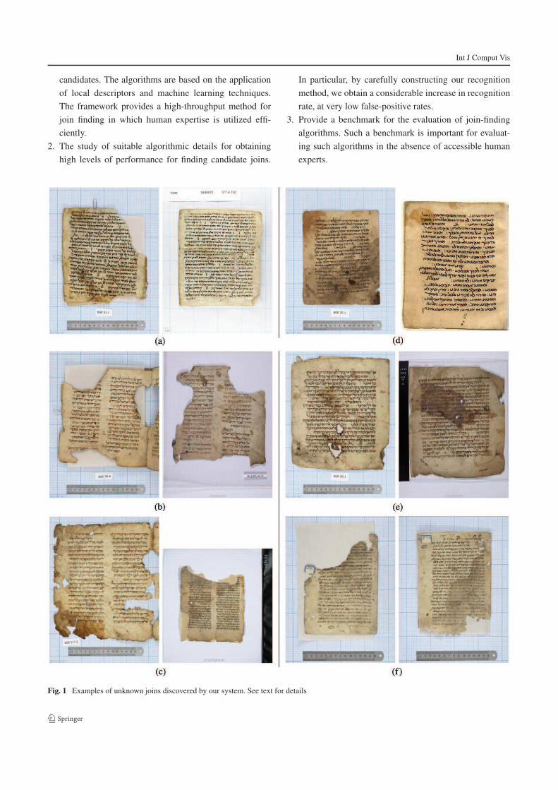
Fig. 1 Examples of unknown joins discovered by our system. See text for details

Int J Comput Vis

4. The actual identification of new, unknown, joins in the

Genizah corpus.

Figure 1 shows a variety of previously-unknown joins

discovered by our method. Example (a) consists of two

leaves from the same copy of the Mishnah, written on vel-

lum in Hebrew in a square script. The texts are from dif-

ferent tractates of Order Zeraim. The left page is from the

recently recovered Geneva collection and the right one from

the small collection of the Jewish National and University

Library. Other leaves from the same manuscript are in Ox-

ford and Cambridge.1 Example (b) shows fragments from a

codex of the Bible, both from the book of Exodus (Hebrew,

square script, on vellum), one from Geneva and the other

from the Jewish Theological Seminary (JTS) in New York,

part of a batch of 69 fragments from various biblical manu-

scripts (partially vocalized and with cantillation signs). Such

codices are written using a very rigid set of typographic

rules, and the identification of such joins based on hand-

writing is considered extremely challenging. Example (c) is

in alternating Hebrew and Aramaic (Targum, square script),

one page from Geneva and the other from the New York JTS

collection. Example (d) shows a join of two leaves of He-

brew liturgical supplications from Geneva and from Penn-

sylvania, in rabbinic script. Example (e) is from a book of

precepts of Saadiah ben Joseph al-Fayyumi, a lost halakhic

work by the 10th century gaon. The left page is from the

Geneva collection and the right one is from JTS. The lan-

guage is Judeo-Arabic, and the text is written in a square

oriental script on vellum. This join is a good example of

how joins can help identify new fragments from lost works.

Once one of the pair is identified correctly, the identification

of the second one is self-determined. Example (f) is from a

responsum in Hebrew (rabbinic script). Both leaves are from

the Alliance Israélite Universelle Library in Paris, but they

are catalogued under different shelfmarks.

2 Related Work

Genizah Research Discovered in 1896 in the attic of a syn-

agogue in the old quarter of Cairo, the Genizah is a large col-

lection of discarded codices, scrolls, and documents, written

mainly in the 10th to 15th centuries. The attic was emptied

and its contents have found their way to over fifty libraries

and collections around the world. The documents, with few

exceptions, are of paper and vellum, and the texts are writ-

ten mainly in Hebrew, Aramaic, and Judeo-Arabic (in He-

brew characters), but also in many other languages (includ-

ing Arabic, Judeo-Spanish, Coptic, Ethiopic, and even one

1It turns out that this specific automatically-proposed join has already

been discovered and is about to be documented in the Sussmann Cata-

log and the Geneva catalog, both going into press now.

in Chinese). The finds included fragments of lost works

(such as the Hebrew original of the apocryphal Book of Ec-

clesiasticus), fragments of hitherto unknown works (such

as the Damascas Document, later found among the Qum-

ran scrolls), and autographs by famous personages, includ-

ing the Andalusians, Yehuda Halevi (1075–1141) and Mai-

monides (1138–1204).

Genizah documents have had an enormous impact on

20th century scholarship in a multitude of fields, includ-

ing Bible, rabbinics, liturgy, history, and philology. Genizah

research has, for example, transformed our understanding

of medieval Mediterranean society and commerce, as ev-

idenced by S.D. Goiten’s monumental five-volume work,

A Mediterranean Society. See Reif (2000) for the history

of the Genizah and of Genizah research. Most of the ma-

terial recovered from the Cairo Genizah has been micro-

filmed and catalogued in the intervening years, but the pho-

tographs are of mediocre quality and the data incomplete

(thousands of fragments are still not listed in published cat-

alogues).

The philanthropically-funded Friedberg Genizah Project

is in the midst of a multi-year process of digitally pho-

tographing (in full color, at 600 dpi) most—if not all—of

the extant manuscripts. The entire collections of the Jewish

Theological Seminary in New York (ENA), the Alliance Is-

raélite Universelle in Paris (AIU), the Jewish National and

University Library (JNUL), the recently rediscovered col-

lection in Geneva, and many smaller collections have al-

ready been digitized, and comprise about 90,000 images

(recto and verso of each fragment). The digital preserva-

tion of another 140,000 fragments at the Taylor-Schechter

Genizah Collection at Cambridge is now underway. The im-

ages are being made available to researchers online at www.

genizah.org.

Unfortunately, most of the leaves that were found were

not found bound together. Worse, many are fragmentary,

whether torn or otherwise mutilated. Pages and fragments

from the same work (book, collection, letter, etc.) may have

found their way to disparate collections around the world.

Some fragments are very difficult to read, as the ink has

faded or the page discolored. Accordingly, scholars have ex-

pended a great deal of time and effort on manually rejoin-

ing leaves of the same original book or pamphlet, and on

piecing together smaller fragments, usually as part of their

research in a particular topic or literary work. Despite the

several thousands of such joins that have been identified by

researchers, very much more remains to be done (Lerner and

Jerchower 2006).

Writer Identification A related task to that of join find-

ing is the task of writer identification, in which the goal

is to identify the writer by morphological characteristics

of a writer’s handwriting. Since historical documents are

Int J Comput Vis

often incomplete and noisy, preprocessing is often ap-

plied to separate the background and to remove noise (see,

for instance, Bres et al. 2006; Leedham et al. 2002). Latin

letters are typically connected, unlike Hebrew ones which

are usually only sporadically connected, and efforts were

also expended on designing segmentation algorithms to dis-

connect letters and facilitate identification. See Casey and

Lecolinet (1996) for a survey of the subject. The identifi-

cation itself is done either by means of local features or

by global statistics. Most recent approaches are of the first

type and identify the writer using letter- or grapheme-based

methods, which use textual feature matching (Panagopoulos

et al. 2009; Bensefia et al. 2003). The work of Bres et al.

(2006) uses text independent statistical features, and Bulacu

and Schomaker (2007), Dinstein and Shapira (1982) com-

bine both local and global statistics.

Interestingly, there is a specialization to individual lan-

guages, employing language-specific letter structure and

morphological characteristics (Bulacu and Schomaker 2007;

Panagopoulos et al. 2009; Dinstein and Shapira 1982). In

our work, we rely on the separation of Hebrew characters by

employing a keypoint detection method that relies on con-

nected components in the thresholded images.

Most of the abovementioned works identify the writer of

the document from a list of known authors. Here, we fo-

cus on finding join candidates, and do not assume a labeled

training set for each join. Note, however, that the techniques

we use are not entirely suitable for distinguishing between

different works of the same writer. Still, since writers are

usually unknown (in the absence of a colophon or signa-

tures), and since joins are the common way to catalog Ge-

nizah documents, we focus on this task. Additional data such

as text or topic identification, page size and number of lines

can be used to help distinguish different works of the same

writer.

The LFW Benchmark To provide a clean computational

framework for the identification of joins, we focus in

our evaluation on the problem of image pair-matching

(same/not-same), and not, for example, on the multiclass

classification problem. Specifically, given images of two

Genizah leaves, our goal is to answer the following sim-

ple question: are these two leaves part of the same original

work or not? Previous studies have shown that improve-

ments obtained on the pair-matching problem carry over to

other recognition tasks (Wolf et al. 2008).

The benchmark we constructed to evaluate our meth-

ods is modeled after the recent Labeled Faces in the Wild

(LFW) face image data set (Huang et al. 2007). The LFW

benchmark has been successful in attracting researchers

to improve face recognition in unconstrained images, and

the results show a gradual improvement over time (Huang

et al. 2008; Wolf et al. 2008, 2009; Pinto et al. 2009;

Taigman et al. 2009; Guillaumin et al. 2009; Kumar et al.

2009), for example; see current results in LFW benchmark

results.

3 Overview

The images used in this study along with accompanying cat-

alogical information are provided by the Friedberg Genizah

Project. The catalogical information is typically incomplete,

and may contain information on the original manuscript,

identification of verified joins, page measurements, approx-

imate date, and literature references.

When found in the Genizah, a manuscript leaf might be

torn into several fragments and is represented by two or

more images depicting the two sides and possibly multiple

images of the same side. The images of each leaf fragment

are marked recto and verso; however, this marking is gener-

ally arbitrary.

The join identification technique follows the following

pipeline depicted in Fig. 2. First, the leaf images are pre-

processed so that each image is segmented into fragments,

and each fragment is binarized and aligned horizontally by

rows. In addition, the page is roughly segmented, and vari-

ous measurements of it are made.

Next, we detect keypoints in the images, and calculate a

descriptor for each keypoint. All descriptors from the same

leaf are combined, and each leaf is then represented by a sin-

gle vector. The vectorization is done by employing a “dictio-

nary” which is computed offline beforehand. Finally, every

pair of vectors (corresponding to two leaves) are compared

by means of a similarity score. We employ both simple and

learned similarity scores and, in addition, combine several

scores together by employing a technique called stacking.

4 Image Processing and Physical Analysis

The images we obtained from the Friedberg Genizah Project

are given as 300–600 dpi JPEGs, of arbitrarily aligned frag-

ments placed on different backgrounds. An example, which

is relatively artifact free, is shown in Fig. 3(a). Many of the

images, however, contain superfluous parts, such as paper

tags, rulers, color tables, etc. (as in Fig. 1). Therefore, a nec-

essary step in our pipeline is preprocessing of the images for

separation of fragments from the background and alignment

of the fragments by the text rows. Then the physical proper-

ties of the fragments and of the text lines are measured.

4.1 Preprocessing

The goal of the preprocessing stage is to eliminate parts of

the images that are irrelevant or may bias the join finding

process, and to prepare the images for the representation

stage.

Int J Comput Vis

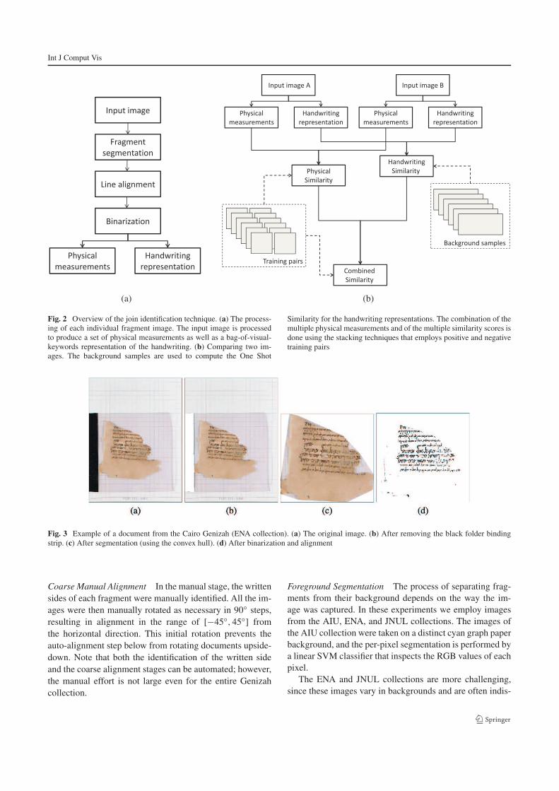
Fig. 2 Overview of the join identification technique. (a) The process-

ing of each individual fragment image. The input image is processed

to produce a set of physical measurements as well as a bag-of-visual-

keywords representation of the handwriting. (b) Comparing two im-

ages. The background samples are used to compute the One Shot

Similarity for the handwriting representations. The combination of the

multiple physical measurements and of the multiple similarity scores is

done using the stacking techniques that employs positive and negative

training pairs

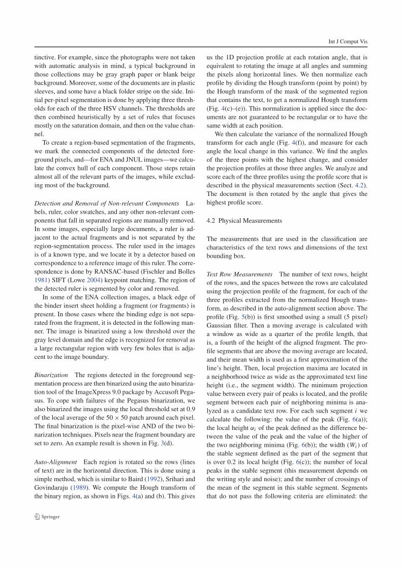
Fig. 3 Example of a document from the Cairo Genizah (ENA collection). (a) The original image. (b) After removing the black folder binding

strip. (c) After segmentation (using the convex hull). (d) After binarization and alignment

Coarse Manual Alignment In the manual stage, the written

sides of each fragment were manually identified. All the im-

ages were then manually rotated as necessary in 90◦ steps,

resulting in alignment in the range of [−45◦,45◦] from

the horizontal direction. This initial rotation prevents the

auto-alignment step below from rotating documents upside-

down. Note that both the identification of the written side

and the coarse alignment stages can be automated; however,

the manual effort is not large even for the entire Genizah

collection.

Foreground Segmentation The process of separating frag-

ments from their background depends on the way the im-

age was captured. In these experiments we employ images

from the AIU, ENA, and JNUL collections. The images of

the AIU collection were taken on a distinct cyan graph paper

background, and the per-pixel segmentation is performed by

a linear SVM classifier that inspects the RGB values of each

pixel.

The ENA and JNUL collections are more challenging,

since these images vary in backgrounds and are often indis-

Int J Comput Vis

tinctive. For example, since the photographs were not taken

with automatic analysis in mind, a typical background in

those collections may be gray graph paper or blank beige

background. Moreover, some of the documents are in plastic

sleeves, and some have a black folder stripe on the side. Ini-

tial per-pixel segmentation is done by applying three thresh-

olds for each of the three HSV channels. The thresholds are

then combined heuristically by a set of rules that focuses

mostly on the saturation domain, and then on the value chan-

nel.

To create a region-based segmentation of the fragments,

we mark the connected components of the detected fore-

ground pixels, and—for ENA and JNUL images—we calcu-

late the convex hull of each component. Those steps retain

almost all of the relevant parts of the images, while exclud-

ing most of the background.

Detection and Removal of Non-relevant Components La-

bels, ruler, color swatches, and any other non-relevant com-

ponents that fall in separated regions are manually removed.

In some images, especially large documents, a ruler is ad-

jacent to the actual fragments and is not separated by the

region-segmentation process. The ruler used in the images

is of a known type, and we locate it by a detector based on

correspondence to a reference image of this ruler. The corre-

spondence is done by RANSAC-based (Fischler and Bolles

1981) SIFT (Lowe 2004) keypoint matching. The region of

the detected ruler is segmented by color and removed.

In some of the ENA collection images, a black edge of

the binder insert sheet holding a fragment (or fragments) is

present. In those cases where the binding edge is not sepa-

rated from the fragment, it is detected in the following man-

ner. The image is binarized using a low threshold over the

gray level domain and the edge is recognized for removal as

a large rectangular region with very few holes that is adja-

cent to the image boundary.

Binarization The regions detected in the foreground seg-

mentation process are then binarized using the auto binariza-

tion tool of the ImageXpress 9.0 package by Accusoft Pega-

sus. To cope with failures of the Pegasus binarization, we

also binarized the images using the local threshold set at 0.9

of the local average of the 50× 50 patch around each pixel.

The final binarization is the pixel-wise AND of the two bi-

narization techniques. Pixels near the fragment boundary are

set to zero. An example result is shown in Fig. 3(d).

Auto-Alignment Each region is rotated so the rows (lines

of text) are in the horizontal direction. This is done using a

simple method, which is similar to Baird (1992), Srihari and

Govindaraju (1989). We compute the Hough transform of

the binary region, as shown in Figs. 4(a) and (b). This gives

us the 1D projection profile at each rotation angle, that is

equivalent to rotating the image at all angles and summing

the pixels along horizontal lines. We then normalize each

profile by dividing the Hough transform (point by point) by

the Hough transform of the mask of the segmented region

that contains the text, to get a normalized Hough transform

(Fig. 4(c)–(e)). This normalization is applied since the doc-

uments are not guaranteed to be rectangular or to have the

same width at each position.

We then calculate the variance of the normalized Hough

transform for each angle (Fig. 4(f)), and measure for each

angle the local change in this variance. We find the angles

of the three points with the highest change, and consider

the projection profiles at those three angles. We analyze and

score each of the three profiles using the profile score that is

described in the physical measurements section (Sect. 4.2).

The document is then rotated by the angle that gives the

highest profile score.

4.2 Physical Measurements

The measurements that are used in the classification are

characteristics of the text rows and dimensions of the text

bounding box.

Text Row Measurements The number of text rows, height

of the rows, and the spaces between the rows are calculated

using the projection profile of the fragment, for each of the

three profiles extracted from the normalized Hough trans-

form, as described in the auto-alignment section above. The

profile (Fig. 5(b)) is first smoothed using a small (5 pixel)

Gaussian filter. Then a moving average is calculated with

a window as wide as a quarter of the profile length, that

is, a fourth of the height of the aligned fragment. The pro-

file segments that are above the moving average are located,

and their mean width is used as a first approximation of the

line’s height. Then, local projection maxima are located in

a neighborhood twice as wide as the approximated text line

height (i.e., the segment width). The minimum projection

value between every pair of peaks is located, and the profile

segment between each pair of neighboring minima is ana-

lyzed as a candidate text row. For each such segment i we

calculate the following: the value of the peak (Fig. 6(a));

the local height αi of the peak defined as the difference be-

tween the value of the peak and the value of the higher of

the two neighboring minima (Fig. 6(b)); the width (Wi ) of

the stable segment defined as the part of the segment that

is over 0.2 its local height (Fig. 6(c)); the number of local

peaks in the stable segment (this measurement depends on

the writing style and noise); and the number of crossings of

the mean of the segment in this stable segment. Segments

that do not pass the following criteria are eliminated: the

Int J Comput Vis

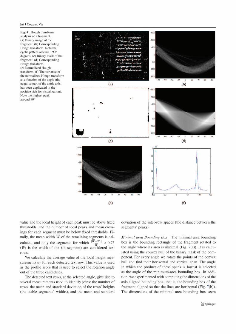
Fig. 4 Hough transform

analysis of a fragment.

(a) Binary image of the

fragment. (b) Corresponding

Hough transform. Note the

cyclic pattern around ±90◦

degrees. (c) Binary mask of the

fragment. (d) Corresponding

Hough transform.

(e) Normalized Hough

transform. (f) The variance of

the normalized Hough transform

as a function of the angle (the

negative part of the angle axis

has been duplicated in the

positive side for visualization).

Note the highest peak

around 90◦

value and the local height of each peak must be above fixed

thresholds, and the number of local peaks and mean cross-

ings for each segment must be below fixed thresholds. Fi-

nally, the mean width W of the remaining segments is cal-

culated, and only the segments for which|W−Wi |

W< 0.75

(Wi is the width of the ith segment) are considered text

rows.

We calculate the average value of the local height mea-

surements αi for each detected text row. This value is used

as the profile score that is used to select the rotation angle

out of the three candidates.

The detected text rows, at the selected angle, give rise to

several measurements used to identify joins: the number of

rows, the mean and standard deviation of the rows’ heights

(the stable segments’ widths), and the mean and standard

deviation of the inter-row spaces (the distance between the

segments’ peaks).

Minimal area Bounding Box The minimal area bounding

box is the bounding rectangle of the fragment rotated to

the angle where its area is minimal (Fig. 7(a)). It is calcu-

lated using the convex hull of the binary mask of the com-

ponent. For every angle we rotate the points of the convex

hull and find their horizontal and vertical span. The angle

in which the product of these spans is lowest is selected

as the angle of the minimum-area bounding box. In addi-

tion, we experimented with computing the dimensions of the

axis aligned bounding box, that is, the bounding box of the

fragment aligned so that the lines are horizontal (Fig. 7(b)).

The dimensions of the minimal area bounding box seem

Int J Comput Vis

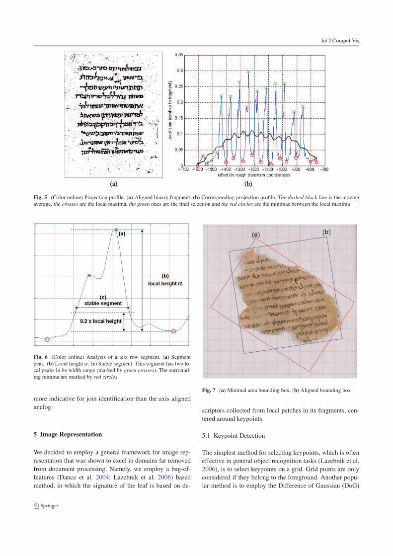
Fig. 5 (Color online) Projection profile. (a) Aligned binary fragment. (b) Corresponding projection profile. The dashed black line is the moving

average, the crosses are the local maxima, the green ones are the final selection and the red circles are the minimas between the local maxima

Fig. 6 (Color online) Analysis of a text row segment. (a) Segment

peak. (b) Local height α. (c) Stable segment. This segment has two lo-

cal peaks in its width range (marked by green crosses). The surround-

ing minima are marked by red circles

more indicative for join identification than the axis aligned

analog.

5 Image Representation

We decided to employ a general framework for image rep-

resentation that was shown to excel in domains far removed

from document processing. Namely, we employ a bag-of-

features (Dance et al. 2004; Lazebnik et al. 2006) based

method, in which the signature of the leaf is based on de-

Fig. 7 (a) Minimal area bounding box. (b) Aligned bounding box

scriptors collected from local patches in its fragments, cen-

tered around keypoints.

5.1 Keypoint Detection

The simplest method for selecting keypoints, which is often

effective in general object recognition tasks (Lazebnik et al.

2006), is to select keypoints on a grid. Grid points are only

considered if they belong to the foreground. Another popu-

lar method is to employ the Difference of Gaussian (DoG)

Int J Comput Vis

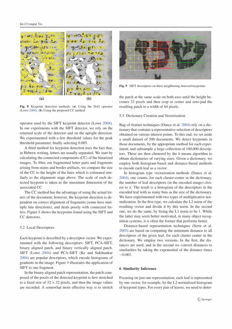
Fig. 8 Keypoint detection methods. (a) Using the DoG operator

(Lowe 2004). (b) Using the proposed CC method

operator used by the SIFT keypoint detector (Lowe 2004).

In our experiments with the SIFT detector, we rely on the

returned scale of the detector and on the upright direction.

We experimented with a few threshold values for the peak

threshold parameter, finally selecting 0.005.

A third method for keypoint detection uses the fact that,

in Hebrew writing, letters are usually separated. We start by

calculating the connected components (CC) of the binarized

images. To filter out fragmented letter parts and fragments

arising from stains and border artifacts, we compare the size

of the CC to the height of the lines which is estimated sim-

ilarly to the alignment stage above. The scale of each de-

tected keypoint is taken as the maximum dimension of the

associated CC.

The CC method has the advantage of using the actual let-

ters of the document; however, the keypoint direction is de-

pendent on correct alignment of fragments (some have mul-

tiple line directions), and deals poorly with connected let-

ters. Figure 8 shows the keypoints found using the SIFT and

CC detectors.

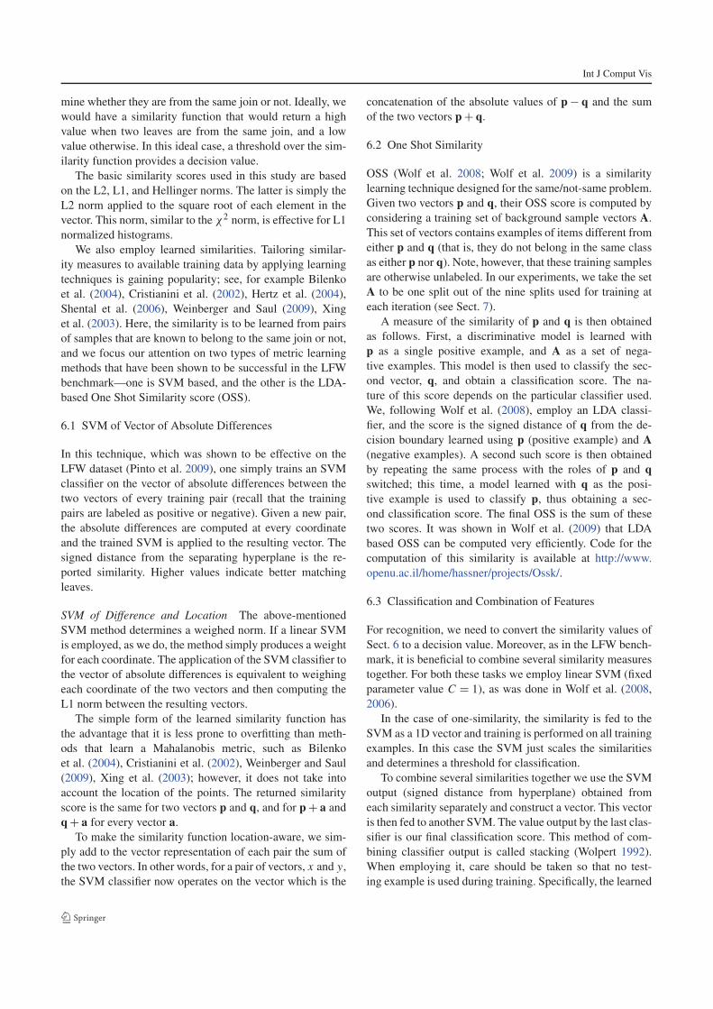
5.2 Local Descriptors

Each keypoint is described by a descriptor vector. We exper-

imented with the following descriptors: SIFT, PCA-SIFT,

binary aligned patch, and binary vertically aligned patch.

SIFT (Lowe 2004) and PCA-SIFT (Ke and Sukthankar

2004) are popular descriptors, which encode histograms of

gradients in the image. Figure 9 illustrates the application of

SIFT to one fragment.

In the binary aligned patch representation, the patch com-

posed of the pixels of the detected keypoint is first stretched

to a fixed size of 32× 32 pixels, and then the image values

are recorded. A somewhat more effective way is to stretch

Fig. 9 SIFT descriptors on three neighboring detected keypoints

the patch at the same scale on both axes until the height be-

comes 32 pixels and then crop or center and zero-pad the

resulting patch to a width of 64 pixels.

5.3 Dictionary Creation and Vectorization

Bag-of-feature techniques (Dance et al. 2004) rely on a dic-

tionary that contains a representative selection of descriptors

obtained on various interest points. To this end, we set aside

a small dataset of 500 documents. We detect keypoints in

those documents, by the appropriate method for each exper-

iment, and subsample a large collection of 100,000 descrip-

tors. These are then clustered by the k-means algorithm to

obtain dictionaries of varying sizes. Given a dictionary, we

employ both histogram-based and distance-based methods

to encode each leaf as a vector.

In histogram type vectorization methods (Dance et al.

2004), one counts, for each cluster-center in the dictionary,

the number of leaf descriptors (in the encoded image) clos-

est to it. The result is a histogram of the descriptors in the

encoded leaf with as many bins as the size of the dictionary.

We have experimented with two types of multiplicative nor-

malization. In the first type, we calculate the L2 norm of the

resulting vector and divide it by this norm. In the second

one, we do the same, by fixing the L1 norm to be 1. While

the latter may seem better motivated, in many object recog-

nition systems, it is often the former that performs better.

Distance-based representation techniques (Serre et al.

2005) are based on computing the minimum distance to all

descriptors of the given leaf, for each cluster center in the

dictionary. We employ two versions. In the first, the dis-

tances are used, and in the second we convert distances to

similarities by taking the exponential of the distance times

−0.001.

6 Similarity Inference

Focusing on just one representation, each leaf is represented

by one vector, for example, by the L2 normalized histogram

of keypoint types. For every pair of leaves, we need to deter-

Int J Comput Vis

mine whether they are from the same join or not. Ideally, we

would have a similarity function that would return a high

value when two leaves are from the same join, and a low

value otherwise. In this ideal case, a threshold over the sim-

ilarity function provides a decision value.

The basic similarity scores used in this study are based

on the L2, L1, and Hellinger norms. The latter is simply the

L2 norm applied to the square root of each element in the

vector. This norm, similar to the χ2 norm, is effective for L1

normalized histograms.

We also employ learned similarities. Tailoring similar-

ity measures to available training data by applying learning

techniques is gaining popularity; see, for example Bilenko

et al. (2004), Cristianini et al. (2002), Hertz et al. (2004),

Shental et al. (2006), Weinberger and Saul (2009), Xing

et al. (2003). Here, the similarity is to be learned from pairs

of samples that are known to belong to the same join or not,

and we focus our attention on two types of metric learning

methods that have been shown to be successful in the LFW

benchmark—one is SVM based, and the other is the LDA-

based One Shot Similarity score (OSS).

6.1 SVM of Vector of Absolute Differences

In this technique, which was shown to be effective on the

LFW dataset (Pinto et al. 2009), one simply trains an SVM

classifier on the vector of absolute differences between the

two vectors of every training pair (recall that the training

pairs are labeled as positive or negative). Given a new pair,

the absolute differences are computed at every coordinate

and the trained SVM is applied to the resulting vector. The

signed distance from the separating hyperplane is the re-

ported similarity. Higher values indicate better matching

leaves.

SVM of Difference and Location The above-mentioned

SVM method determines a weighed norm. If a linear SVM

is employed, as we do, the method simply produces a weight

for each coordinate. The application of the SVM classifier to

the vector of absolute differences is equivalent to weighing

each coordinate of the two vectors and then computing the

L1 norm between the resulting vectors.

The simple form of the learned similarity function has

the advantage that it is less prone to overfitting than meth-

ods that learn a Mahalanobis metric, such as Bilenko

et al. (2004), Cristianini et al. (2002), Weinberger and Saul

(2009), Xing et al. (2003); however, it does not take into

account the location of the points. The returned similarity

score is the same for two vectors p and q, and for p + a and

q + a for every vector a.

To make the similarity function location-aware, we sim-

ply add to the vector representation of each pair the sum of

the two vectors. In other words, for a pair of vectors, x and y,

the SVM classifier now operates on the vector which is the

concatenation of the absolute values of p − q and the sum

of the two vectors p + q.

6.2 One Shot Similarity

OSS (Wolf et al. 2008; Wolf et al. 2009) is a similarity

learning technique designed for the same/not-same problem.

Given two vectors p and q, their OSS score is computed by

considering a training set of background sample vectors A.

This set of vectors contains examples of items different from

either p and q (that is, they do not belong in the same class

as either p nor q). Note, however, that these training samples

are otherwise unlabeled. In our experiments, we take the set

A to be one split out of the nine splits used for training at

each iteration (see Sect. 7).

A measure of the similarity of p and q is then obtained

as follows. First, a discriminative model is learned with

p as a single positive example, and A as a set of nega-

tive examples. This model is then used to classify the sec-

ond vector, q, and obtain a classification score. The na-

ture of this score depends on the particular classifier used.

We, following Wolf et al. (2008), employ an LDA classi-

fier, and the score is the signed distance of q from the de-

cision boundary learned using p (positive example) and A

(negative examples). A second such score is then obtained

by repeating the same process with the roles of p and q

switched; this time, a model learned with q as the posi-

tive example is used to classify p, thus obtaining a sec-

ond classification score. The final OSS is the sum of these

two scores. It was shown in Wolf et al. (2009) that LDA

based OSS can be computed very efficiently. Code for the

computation of this similarity is available at http://www.

openu.ac.il/home/hassner/projects/Ossk/.

6.3 Classification and Combination of Features

For recognition, we need to convert the similarity values of

Sect. 6 to a decision value. Moreover, as in the LFW bench-

mark, it is beneficial to combine several similarity measures

together. For both these tasks we employ linear SVM (fixed

parameter value C = 1), as was done in Wolf et al. (2008,

2006).

In the case of one-similarity, the similarity is fed to the

SVM as a 1D vector and training is performed on all training

examples. In this case the SVM just scales the similarities

and determines a threshold for classification.

To combine several similarities together we use the SVM

output (signed distance from hyperplane) obtained from

each similarity separately and construct a vector. This vector

is then fed to another SVM. The value output by the last clas-

sifier is our final classification score. This method of com-

bining classifier output is called stacking (Wolpert 1992).

When employing it, care should be taken so that no test-

ing example is used during training. Specifically, the learned

Int J Comput Vis

similarities above (SVM-based and OSS) need to be com-

puted multiple times.

7 The Newly Proposed Genizah Benchmark

Our benchmark, which is modeled after the LFW face recog-

nition benchmark (Huang et al. 2007), consists of 31,315

leaves, all from the New York (ENA), Paris (AIU), and

Jerusalem (JNUL) collections. There are several differences

vis-à-vis the LFW benchmark. First, in the LFW benchmark

the number of positive pairs (images of the same person)

and the number of negative pairs are equal. In our bench-

mark, this is not the case, since the number of known joins is

rather limited. Second, while in the LFW benchmark, a neg-

ative pair is a pair that is known to be negative, in our case a

negative pair is a pair that is not known to be positive. This

should not pose a major problem, since the expected number

of unknown joins is very limited in comparison to the total

number of pairs.

There are two views of the dataset: View 1, which is

meant for parameter tuning, and View 2, meant for reporting

results. View 1 contains three splits, each containing 1000

positive pairs of leaves belonging each to the same join, and

2000 negative pairs of leaves that are not known to belong to

the same join. When working on View 1, one trains on two

splits and tests on the third.

View 2 of the benchmark consists of ten equally sized

sets. Each also contains 1000 positive pairs of images taken

from the same joins, and 2000 negative pairs. Care is taken

so that no known join appears in more than one set, and that

the number of positive pairs taken from one join does not

exceed 20.

To report results on View 2, one repeats the classifica-

tion process 10 times. In each iteration, nine sets are taken

as training, and the results are evaluated on the 10th set. Re-

sults are reported by constructing an ROC curve for all splits

together (the outcome value for each pair is computed when

this pair is a testing pair), by computing statistics of the ROC

curve (area under curve, equal error rate, and true positive

rate at a certain low false positive rate) and by recording av-

erage recognition rate for the 10 splits.

7.1 Results Obtained on the New Benchmark

To determine the best methods and settings for join identi-

fication, we have experimented with the various aspects of

the algorithm. When varying one aspect, we fixed the others

to the following default values: the connected component

method for keypoint selection algorithm, the SIFT descrip-

tor, a dictionary size of 500, L2 normalized histogram for

vectorization, and SVM applied to absolute difference be-

tween vectors as the similarity measure.

Results for the parametric methods (keypoint detection

method, descriptor type and parameters and dictionary size)

were compared on View 1. Results for the various norms and

vectorization methods were compared on View 2, since they

do not require fitting of parameters.

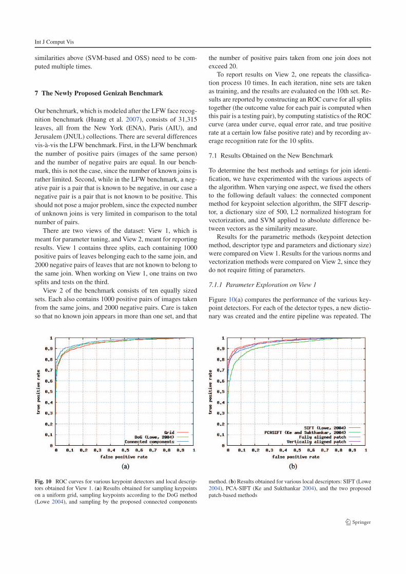
7.1.1 Parameter Exploration on View 1

Figure 10(a) compares the performance of the various key-

point detectors. For each of the detector types, a new dictio-

nary was created and the entire pipeline was repeated. The

Fig. 10 ROC curves for various keypoint detectors and local descrip-

tors obtained for View 1. (a) Results obtained for sampling keypoints

on a uniform grid, sampling keypoints according to the DoG method

(Lowe 2004), and sampling by the proposed connected components

method. (b) Results obtained for various local descriptors: SIFT (Lowe

2004), PCA-SIFT (Ke and Sukthankar 2004), and the two proposed

patch-based methods

Int J Comput Vis

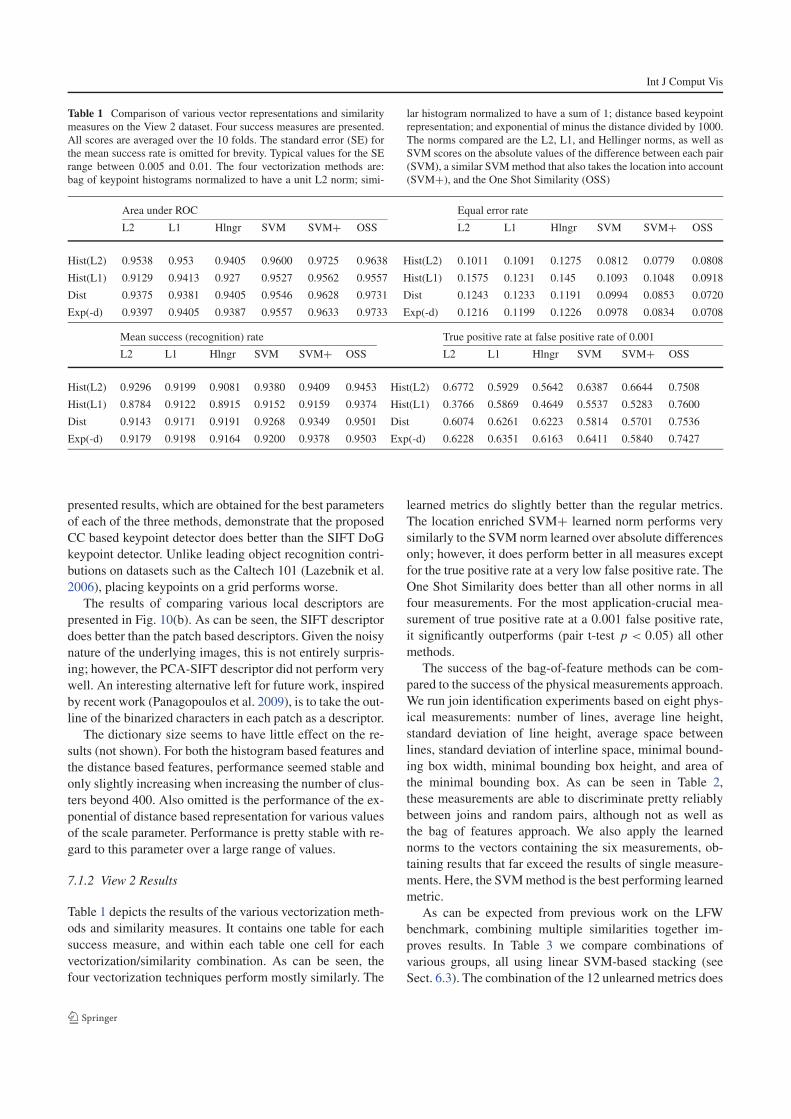
Table 1 Comparison of various vector representations and similarity

measures on the View 2 dataset. Four success measures are presented.

All scores are averaged over the 10 folds. The standard error (SE) for

the mean success rate is omitted for brevity. Typical values for the SE

range between 0.005 and 0.01. The four vectorization methods are:

bag of keypoint histograms normalized to have a unit L2 norm; simi-

lar histogram normalized to have a sum of 1; distance based keypoint

representation; and exponential of minus the distance divided by 1000.

The norms compared are the L2, L1, and Hellinger norms, as well as

SVM scores on the absolute values of the difference between each pair

(SVM), a similar SVMmethod that also takes the location into account

(SVM+), and the One Shot Similarity (OSS)

Area under ROC Equal error rate

L2 L1 Hlngr SVM SVM+ OSS L2 L1 Hlngr SVM SVM+ OSS

Hist(L2) 0.9538 0.953 0.9405 0.9600 0.9725 0.9638 Hist(L2) 0.1011 0.1091 0.1275 0.0812 0.0779 0.0808

Hist(L1) 0.9129 0.9413 0.927 0.9527 0.9562 0.9557 Hist(L1) 0.1575 0.1231 0.145 0.1093 0.1048 0.0918

Dist 0.9375 0.9381 0.9405 0.9546 0.9628 0.9731 Dist 0.1243 0.1233 0.1191 0.0994 0.0853 0.0720

Exp(-d) 0.9397 0.9405 0.9387 0.9557 0.9633 0.9733 Exp(-d) 0.1216 0.1199 0.1226 0.0978 0.0834 0.0708

Mean success (recognition) rate True positive rate at false positive rate of 0.001

L2 L1 Hlngr SVM SVM+ OSS L2 L1 Hlngr SVM SVM+ OSS

Hist(L2) 0.9296 0.9199 0.9081 0.9380 0.9409 0.9453 Hist(L2) 0.6772 0.5929 0.5642 0.6387 0.6644 0.7508

Hist(L1) 0.8784 0.9122 0.8915 0.9152 0.9159 0.9374 Hist(L1) 0.3766 0.5869 0.4649 0.5537 0.5283 0.7600

Dist 0.9143 0.9171 0.9191 0.9268 0.9349 0.9501 Dist 0.6074 0.6261 0.6223 0.5814 0.5701 0.7536

Exp(-d) 0.9179 0.9198 0.9164 0.9200 0.9378 0.9503 Exp(-d) 0.6228 0.6351 0.6163 0.6411 0.5840 0.7427

presented results, which are obtained for the best parameters

of each of the three methods, demonstrate that the proposed

CC based keypoint detector does better than the SIFT DoG

keypoint detector. Unlike leading object recognition contri-

butions on datasets such as the Caltech 101 (Lazebnik et al.

2006), placing keypoints on a grid performs worse.

The results of comparing various local descriptors are

presented in Fig. 10(b). As can be seen, the SIFT descriptor

does better than the patch based descriptors. Given the noisy

nature of the underlying images, this is not entirely surpris-

ing; however, the PCA-SIFT descriptor did not perform very

well. An interesting alternative left for future work, inspired

by recent work (Panagopoulos et al. 2009), is to take the out-

line of the binarized characters in each patch as a descriptor.

The dictionary size seems to have little effect on the re-

sults (not shown). For both the histogram based features and

the distance based features, performance seemed stable and

only slightly increasing when increasing the number of clus-

ters beyond 400. Also omitted is the performance of the ex-

ponential of distance based representation for various values

of the scale parameter. Performance is pretty stable with re-

gard to this parameter over a large range of values.

7.1.2 View 2 Results

Table 1 depicts the results of the various vectorization meth-

ods and similarity measures. It contains one table for each

success measure, and within each table one cell for each

vectorization/similarity combination. As can be seen, the

four vectorization techniques perform mostly similarly. The

learned metrics do slightly better than the regular metrics.

The location enriched SVM+ learned norm performs very

similarly to the SVM norm learned over absolute differences

only; however, it does perform better in all measures except

for the true positive rate at a very low false positive rate. The

One Shot Similarity does better than all other norms in all

four measurements. For the most application-crucial mea-

surement of true positive rate at a 0.001 false positive rate,

it significantly outperforms (pair t-test p < 0.05) all other

methods.

The success of the bag-of-feature methods can be com-

pared to the success of the physical measurements approach.

We run join identification experiments based on eight phys-

ical measurements: number of lines, average line height,

standard deviation of line height, average space between

lines, standard deviation of interline space, minimal bound-

ing box width, minimal bounding box height, and area of

the minimal bounding box. As can be seen in Table 2,

these measurements are able to discriminate pretty reliably

between joins and random pairs, although not as well as

the bag of features approach. We also apply the learned

norms to the vectors containing the six measurements, ob-

taining results that far exceed the results of single measure-

ments. Here, the SVMmethod is the best performing learned

metric.

As can be expected from previous work on the LFW

benchmark, combining multiple similarities together im-

proves results. In Table 3 we compare combinations of

various groups, all using linear SVM-based stacking (see

Sect. 6.3). The combination of the 12 unlearned metrics does

Int J Comput Vis

Table 2 Comparison of various

physical measurements on the

View 2 dataset. The learned

metrics SVM, SVM+, and OSS

are employed between pairs of

8D vectors containing the

physical measurements. Note

that since the measurements

have outliers, it happens for

many of the rows that the SVM

classifier used to determine the

threshold value sets it such that

all examples are predicted as

negative. As is clear from the

three other scores, using a

different threshold, the

prediction is not random

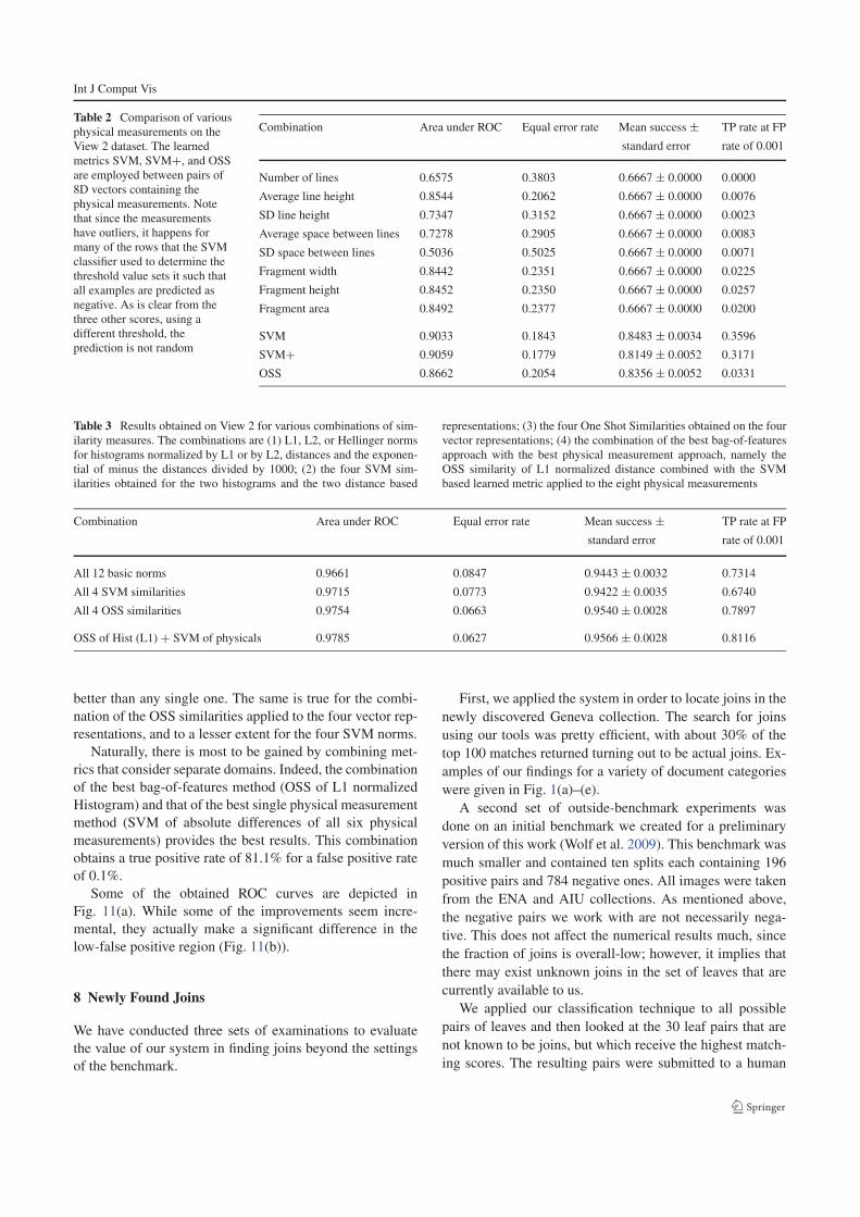
Combination Area under ROC Equal error rate Mean success ± TP rate at FP

standard error rate of 0.001

Number of lines 0.6575 0.3803 0.6667 ± 0.0000 0.0000

Average line height 0.8544 0.2062 0.6667 ± 0.0000 0.0076

SD line height 0.7347 0.3152 0.6667 ± 0.0000 0.0023

Average space between lines 0.7278 0.2905 0.6667 ± 0.0000 0.0083

SD space between lines 0.5036 0.5025 0.6667 ± 0.0000 0.0071

Fragment width 0.8442 0.2351 0.6667 ± 0.0000 0.0225

Fragment height 0.8452 0.2350 0.6667 ± 0.0000 0.0257

Fragment area 0.8492 0.2377 0.6667 ± 0.0000 0.0200

SVM 0.9033 0.1843 0.8483 ± 0.0034 0.3596

SVM+ 0.9059 0.1779 0.8149 ± 0.0052 0.3171

OSS 0.8662 0.2054 0.8356 ± 0.0052 0.0331

Table 3 Results obtained on View 2 for various combinations of sim-

ilarity measures. The combinations are (1) L1, L2, or Hellinger norms

for histograms normalized by L1 or by L2, distances and the exponen-

tial of minus the distances divided by 1000; (2) the four SVM sim-

ilarities obtained for the two histograms and the two distance based

representations; (3) the four One Shot Similarities obtained on the four

vector representations; (4) the combination of the best bag-of-features

approach with the best physical measurement approach, namely the

OSS similarity of L1 normalized distance combined with the SVM

based learned metric applied to the eight physical measurements

Combination Area under ROC Equal error rate Mean success ± TP rate at FP

standard error rate of 0.001

All 12 basic norms 0.9661 0.0847 0.9443 ± 0.0032 0.7314

All 4 SVM similarities 0.9715 0.0773 0.9422 ± 0.0035 0.6740

All 4 OSS similarities 0.9754 0.0663 0.9540 ± 0.0028 0.7897

OSS of Hist (L1) + SVM of physicals 0.9785 0.0627 0.9566 ± 0.0028 0.8116

better than any single one. The same is true for the combi-

nation of the OSS similarities applied to the four vector rep-

resentations, and to a lesser extent for the four SVM norms.

Naturally, there is most to be gained by combining met-

rics that consider separate domains. Indeed, the combination

of the best bag-of-features method (OSS of L1 normalized

Histogram) and that of the best single physical measurement

method (SVM of absolute differences of all six physical

measurements) provides the best results. This combination

obtains a true positive rate of 81.1% for a false positive rate

of 0.1%.

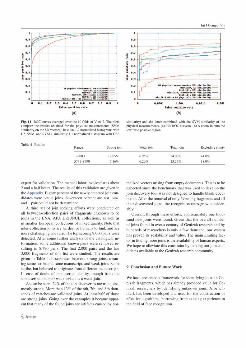
Some of the obtained ROC curves are depicted in

Fig. 11(a). While some of the improvements seem incre-

mental, they actually make a significant difference in the

low-false positive region (Fig. 11(b)).

8 Newly Found Joins

We have conducted three sets of examinations to evaluate

the value of our system in finding joins beyond the settings

of the benchmark.

First, we applied the system in order to locate joins in the

newly discovered Geneva collection. The search for joins

using our tools was pretty efficient, with about 30% of the

top 100 matches returned turning out to be actual joins. Ex-

amples of our findings for a variety of document categories

were given in Fig. 1(a)–(e).

A second set of outside-benchmark experiments was

done on an initial benchmark we created for a preliminary

version of this work (Wolf et al. 2009). This benchmark was

much smaller and contained ten splits each containing 196

positive pairs and 784 negative ones. All images were taken

from the ENA and AIU collections. As mentioned above,

the negative pairs we work with are not necessarily nega-

tive. This does not affect the numerical results much, since

the fraction of joins is overall-low; however, it implies that

there may exist unknown joins in the set of leaves that are

currently available to us.

We applied our classification technique to all possible

pairs of leaves and then looked at the 30 leaf pairs that are

not known to be joins, but which receive the highest match-

ing scores. The resulting pairs were submitted to a human

Int J Comput Vis

Fig. 11 ROC curves averaged over the 10 folds of View 2. The plots

compare the results obtained for the physical measurements (SVM

similarity on the 8D vectors); baseline L2 normalized histograms with

L2, SVM, and SVM+ similarity; L1 normalized histogram with OSS

similarity; and the latter combined with the SVM similarity of the

physical measurements. (a) Full ROC curvesõ. (b) A zoom-in onto the

low false positive region

Table 4 ResultsRange Strong join Weak join Total join Excluding empty

1–2000 17.05% 6.95% 24.00% 44.8%

5791–8790 7.16% 6.20% 13.37% 18.0%

expert for validation. The manual labor involved was about

2 and a half hours. The results of this validation are given in

the Appendix. Eighty percent of the newly detected join can-

didates were actual joins. Seventeen percent are not joins,

and 1 pair could not be determined.

A third set of join seeking efforts were conducted on

all between-collection pairs of fragments unknown to be

joins in the ENA, AIU, and JNUL collections, as well as

in smaller European collections of mixed quality. Note that

inter-collection joins are harder for humans to find, and are

more challenging and rare. The top scoring 9,000 pairs were

detected. After some further analysis of the catalogical in-

formation, some additional known pairs were removed re-

sulting in 8,790 pairs. The first 2,000 pairs and the last

3,000 fragments of this list were studied. The results are

given in Table 4. It separates between strong joins, mean-

ing same scribe and same manuscript, and weak joins–same

scribe, but believed to originate from different manuscripts.

In case of doubt of manuscript identity, though from the

same scribe, the pair was marked as a weak join.

As can be seen, 24% of the top discoveries are true joins,

mostly strong. More than 13% of the 6th, 7th, and 8th thou-

sands of matches are validated joins. At least half of those

are strong joins. Going over the examples it became appar-

ent that many of the found joins are artifacts caused by nor-

malized vectors arising from empty documents. This is to be

expected since the benchmark that was used to develop the

join discovery tool was not designed to handle blank docu-

ments. After the removal of only 49 empty fragments and all

their discovered joins, the recognition rates grew consider-

ably.

Overall, through these efforts, approximately one thou-

sand new joins were found. Given that the overall number

of joins found in over a century of Genizah research and by

hundreds of researchers is only a few thousand, our system

has proven its scalability and value. The main limiting fac-

tor in finding more joins is the availability of human experts.

We hope to alleviate this constraint by making our join can-

didates available to the Genizah research community.

9 Conclusion and Future Work

We have presented a framework for identifying joins in Ge-

nizah fragments, which has already provided value for Ge-

nizah researchers by identifying unknown joins. A bench-

mark has been developed and used for the construction of

effective algorithms, borrowing from existing experience in

the field of face recognition.

Int J Comput Vis

We are making our benchmark, together with the original

and processed images and encodings, available for the rest

of the community in order to facilitate the effective develop-

ment of better algorithms in the future.

9.1 Future Work

The high-resolution scanning of the Genizah documents is

still taking place, and so far we were able to examine only

about 20% of the fragments known to exist, examining less

than 4% of the join potential. Note, however, that the meth-

ods we employ are efficient and may be employed to the

entire corpus in due time.

Our future research plans focus on improving all aspects

of the algorithms, as well as including new sources of infor-

mation such as analysis of the shape of the fragment (frag-

ments of the same join are likely to have the same overall

shapes and holes), and the automatic classification of frag-

ment material (paper/vellum).

We are also looking at alternative ways to find similarity

between Genizah images. An interesting direction, due to

Mica Arie-Nachmison (personal communication), would be

to consider patch based composition approaches in compar-

ing two fragments. Two fragment images would be believed

to be compatible if one can compose the written area of one

image from the written area of another. This is exactly what

is being measured by the bidirectional similarity function

(Simakov et al. 2008). Initial experiments done with the ran-

domized implementation of Barnes et al. (2009) show that

this method might assist in identifying joins; however, the

results are still not on a par with the bag-of-features results.

The obtained Area Under Curve is 0.63, and the Equal Error

Rate is 0.31.

Another avenue of future research is the construction of

a paleographic tool that, given a fragment, will provide suit-

able candidates for matching writing styles and dates. Such a

tool will expedite the paleographic classification of the frag-

ments, and will assist the join finding process (the analog in

faces would be the recognition of facial traits (Wolf et al.

2009; Kumar et al. 2009) to facilitate better face identifica-

tion). For the construction of this tool, we plan to use writing

samples from various locale and times available in the pale-

ographic literature.

Acknowledgements We would like to thank Dr. Dov Friedberg for a

generous grant that enabled us to start this research, and the Friedberg

Genizah Project for matching funds that enabled its continuation.

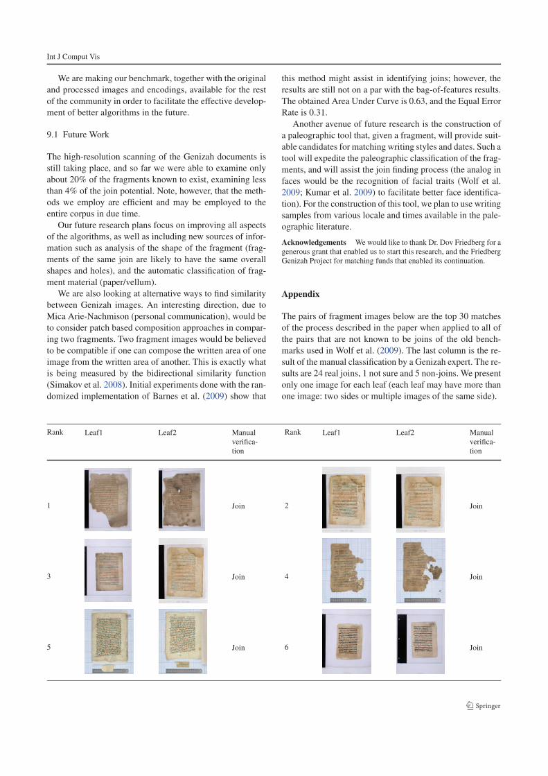
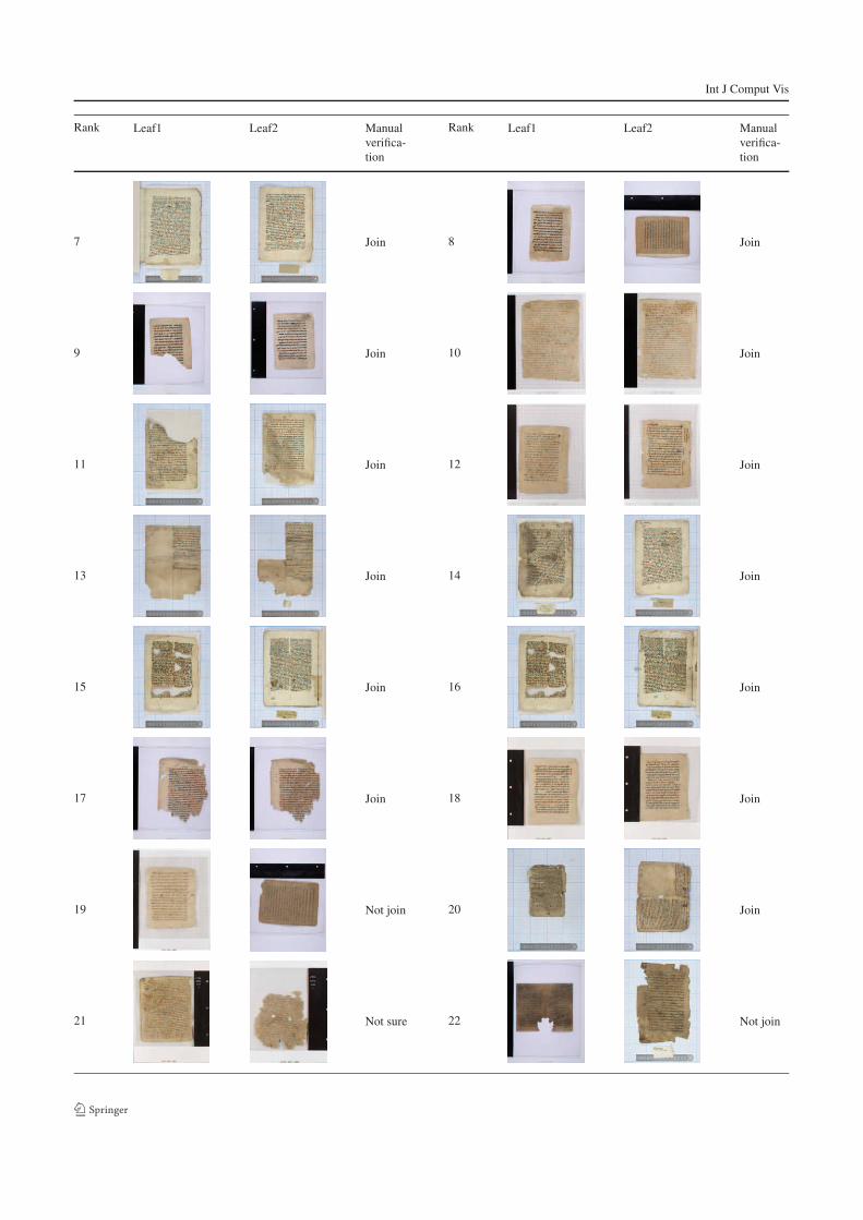
Appendix

The pairs of fragment images below are the top 30 matches

of the process described in the paper when applied to all of

the pairs that are not known to be joins of the old bench-

marks used in Wolf et al. (2009). The last column is the re-

sult of the manual classification by a Genizah expert. The re-

sults are 24 real joins, 1 not sure and 5 non-joins. We present

only one image for each leaf (each leaf may have more than

one image: two sides or multiple images of the same side).

Rank Leaf1 Leaf2 Rank Leaf1 Leaf2Manual

verifica-

tion

Manual

verifica-

tion

1 Join 2 Join

3 Join 4 Join

5 Join 6 Join

Int J Comput Vis

Rank Leaf1 Leaf2 Rank Leaf1 Leaf2Manual

verifica-

tion

Manual

verifica-

tion

7 Join 8 Join

9 Join 10 Join

11 Join 12 Join

13 Join 14 Join

15 Join 16 Join

17 Join 18 Join

19 Not join 20 Join

21 Not sure 22 Not join

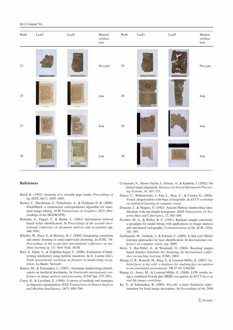
Int J Comput Vis

Rank Leaf1 Leaf2 Rank Leaf1 Leaf2Manual

verifica-

tion

Manual

verifica-

tion

23 Not join 24 Not join

25 Join 26 Join

27 Join 28 Join

29 Join 30 Join

References

Baird, K. (1992). Anatomy of a versatile page reader. Proceedings of

the IEEE, 80(7), 1059–1065.

Barnes, C., Shechtman, E., Finkelstein, A., & Goldman, D. B. (2009).

PatchMatch: a randomized correspondence algorithm for struc-

tural image editing. ACM Transactions on Graphics, 28(3) (Pro-

ceedings of the SIGGRAPH)

Bensefia, A., Paquet, T., & Heutte, L. (2003). Information retrieval

based writer identification. In Proceedings of the seventh inter-

national conference on document analysis and recognition (pp.

946–950).

Bilenko, M., Basu, S., & Mooney, R. J. (2004). Integrating constraints

and metric learning in semi-supervised clustering. In ICML ’04:

Proceedings of the twenty-first international conference on ma-

chine learning (p. 11). New York: ACM.

Bres, S., Eglin, V., & VolpilhacAuger, C. (2006). Evaluation of hand-

writing similarities using hermite transform. In G. Lorette (Ed.),

Tenth international workshop on frontiers in handwriting recog-

nition. La Baule: Suvisoft.

Bulacu, M., & Schomaker, L. (2007). Automatic handwriting identifi-

cation on medieval documents. In Fourteenth international con-

ference on image analysis and processing, ICIAP (pp. 279–284).

Casey, R., & Lecolinet, E. (1996). A survey of methods and strategies

in character segmentation. IEEE Transactions on Pattern Analysis

and Machine Intelligence, 18(7), 690–706.

Cristianini, N., Shawe-Taylor, J., Elissee, A., & Kandola, J. (2002). On

kernel-target alignment. Advances in Neural Information Process-

ing Systems, 14, 367–373.

Dance, C., Willamowski, J., Fan, L., Bray, C., & Csurka, G. (2004).

Visual categorization with bags of keypoints. In ECCV workshop

on statistical learning in computer vision.

Dinstein, I., & Shapira, Y. (1982). Ancient Hebraic handwriting iden-

tification with run-length histograms. IEEE Transactions on Sys-

terms Man and Cybernetics, 12, 405–409.

Fischler, M. A., & Bolles, R. C. (1981). Random sample consensus:

a paradigm for model fitting with applications to image analysis

and automated cartography. Communications of the ACM, 24(6),

381–395.

Guillaumin, M., Verbeek, J., & Schmid, C. (2009). Is that you? Metric

learning approaches for face identification. In International con-

ference on computer vision, sep. 2009.

Hertz, T., Bar-Hillel, A., & Weinshall, D. (2004). Boosting margin

based distance functions for clustering. In International confer-

ence on machine learning, ICML, 2004.

Huang, G. B., Ramesh, M., Berg, T., & Learned-Miller, E. (2007). La-

beled faces in the wild: a database for studying face recognition

in unconstrained environments. TR 07-49, UMASS.

Huang, G., Jones, M., & Learned-Miller, E. (2008). LFW results us-

ing a combined Nowak plus MERL recognizer. In ECCV faces in

real-life images workshop.

Ke, Y., & Sukthankar, R. (2004). Pca-sift: a more distinctive repre-

sentation for local image descriptors. In Proceedings of the 2004

Int J Comput Vis

IEEE computer society conference on computer vision and pat-

tern recognition, CVPR 2004 (Vol. 2, pp. II–506–II–513)

Kumar, N., Berg, A. C., Belhumeur, P. N., & Nayar, S. K. (2009). At-

tribute and simile classifiers for face verification. In IEEE inter-

national conference on computer vision, ICCV, Oct. 2009.

Lazebnik, S., Schmid, C., & Ponce, J. (2006). Beyond bags of fea-

tures: spatial pyramid matching for recognizing natural scene cat-

egories. In 2006 IEEE computer society conference on computer

vision and pattern recognition (Vol. 2, pp. 2169–2178)

Leedham, G., Varma, S., Patankar, A., & Govindarayu, V. (2002).

Separating text and background in degraded document images;

a comparison of global threshholding techniques for multi-stage

threshholding. In International workshop on frontiers in hand-

writing recognition (pp. 244–249).

Lerner, H. G., & Jerchower, S. (2006). The Penn/Cambridge Genizah

fragment project: issues in description, access, and reunification.

Cataloging & Classification Quarterly, 42(1), 21–39.

LFW benchmark results. http://vis-www.cs.umass.edu/lfw/results.

html.

Lowe, D. G. (2004). Distinctive image features from scale-invariant

keypoints. International Journal of Computer Vision, 60(2), 91–

110.

Panagopoulos, M., Papaodysseus, C., Rousopoulos, P., Dafi, D., &

Tracy, S. (2009). Automatic writer identification of ancient Greek

inscriptions. IEEE Transactions on Pattern Analysis and Machine

Intelligence, 31(8), 1404–1414.

Pinto, N., DiCarlo, J., & Cox, D. (2009). How far can you get with

a modern face recognition test set using only simple features? In

IEEE computer society conference on computer vision and pat-

tern recognition, pp. 2591–2598

Reif, S. C. (2000). A Jewish archive from Old Cairo: the history of

Cambridge University’s Genizah collection. Richmond: Curzon

Press.

Serre, T., Wolf, L., & Poggio, T. (2005). Object recognition with fea-

tures inspired by visual cortex. In IEEE computer society confer-

ence on computer vision and pattern recognition, CVPR (Vol. 2,

pp. 994–1000).

Shental, N., Hertz, T., Weinshall, D., & Pavel, M. (2006). Adjustment

learning and relevant component analysis. In Computer vision,

ECCV (pp. 181–185).

Simakov, D., Caspi, Y., Shechtman, E., & Irani, M. (2008). Summariz-

ing visual data using bidirectional similarity. In IEEE conference

on computer vision and pattern recognition, CVPR 2008 (pp. 1–

8).

Srihari, S. N., & Govindaraju, V. (1989). Analysis of textual images us-

ing the Hough transform. Machine Vision and Applications, 2(3),

141–153.

Taigman, Y., Wolf, L., & Hassner, T. (2009). Multiple one-shots for

utilizing class label information. In The British machine vision

conference, BMVC, Sept. 2009.

Weinberger, K. Q., & Saul, L. K. (2009). Distance metric learning for

large margin nearest neighbor classification. Journal of Machine

Learning Research, 10, 207–244.

Wolf, L., Bileschi, S., & Meyers, E. (2006). Perception strategies in

hierarchical vision systems. In 2006 IEEE computer society con-

ference on computer vision and pattern recognition (Vol. 2, pp.

2153–2160).

Wolf, L., Hassner, T., & Taigman, Y. (2008). Descriptor based methods

in the wild. In Faces in real-life images workshop in ECCV.

Wolf, L., Hassner, T., & Taigman, Y. (2009). The one-shot similar-

ity kernel. In IEEE international conference on computer vision,

ICCV, Sept. 2009.

Wolf, L., Littman, R., Mayer, N., Dershowitz, N., Shweka, R., &

Choueka, Y. (2009). Automatically identifying join candidates in

the Cairo Genizah. In Post ICCV workshop on eHeritage and dig-

ital art preservation, Sept. 2009.

Wolf, L., Taigman, Y., & Hassner, T. (2009). Similarity scores based

on background samples. In Asian computer vision conference,

ACCV, Sept. 2009.

Wolpert, D. H. (1992). Stacked generalization. Neural Networks, 5(2),

241–259.

Xing, E., Ng, A. Y., Jordan, M., & Russell, S. (2003). Distance metric

learning, with application to clustering with side-information. In

NIPS.