Identifying and Communicating Genetic Determinants of ... · 1 Final Technical Report for NIJ grant 2008-DN-BX-K125, “Identifying and Communicating Genetic Determinants of Facial

The author(s) shown below used Federal funds provided by the U.S. Department of Justice and prepared the following final report: Document Title: Identifying and Communicating Genetic

Determinants of Facial Features: Practical Considerations in Forensic Molecular Photofitting

Author(s): Mark Shriver Document No.: 248591 Date Received: January 2015 Award Number: 2008-DN-BX-K125 This report has not been published by the U.S. Department of Justice. To provide better customer service, NCJRS has made this Federally-funded grant report available electronically.

Opinions or points of view expressed are those of the author(s) and do not necessarily reflect

the official position or policies of the U.S. Department of Justice.

1

Final Technical Report for NIJ grant 2008-DN-BX-K125, “Identifying and Communicating

Genetic Determinants of Facial Features: Practical Considerations in Forensic Molecular

Photofitting”

By: Mark Shriver, Project PI

Date: July 26, 2013

This document represents the executive of the technical report for the above noted NIJ

fundedresearch project that was carried out at Penn State University. The initial specific aims as

listed in the funded research proposal are:

The primary goals (specific aims) of this proposed research are:

1. Identify genes underlying variability in facial features within and among European and

West Africans populations. This aim includes population sample collection, phenotyping

of 3D photos, whole-genome marker genotyping, and gene mapping.

2. Assay independent population samples to test for replication of significant mapping

results. Replication of whole genome mapping results is critically important especially

for complex and multifaceted traits like human facial features.

3. Test for the ability of human observers to recognize the effects of individual genes on

facial features and to match facial photographs with corresponding computer-generated

facial reconstructions based on functional locus genotype.

We have accomplished these aims, which have been documented in a Ph.D. dissertation

successfully defended by Denise Liberton, “An Investigation into Genes Underlying Normal

Variation in Facial Morphology in Admixed Populations” and this final technical report. Note

that many of the results in this technical report are currently unpublished and a manuscript is

reporting on these results is in review. As such this technical report should be considered a

CONFIDENTIAL COMMUNICATION AND SHOULD NOT BE DISTRIBUTED

OUTSIDE OF THE NIJ WITHOUT MY NOTIFICATION.

This report is organized in two major sections: First is a concise description of the major results

and findings, the Executive Summary. Second is a more technically detailed materials and

methods section, the Executive Technical Report. The table of contents is on page 3 and a

glossary of terms appears on pages 12-13.

This document is a research report submitted to the U.S. Department of Justice. This report has not been published by the Department. Opinions or points of view expressed are those of the author(s)

and do not necessarily reflect the official position or policies of the U.S. Department of Justice.

2

This work summarizes the joint effort of a number of people across several countries and has

been supported by several foundations and US federal agencies and the Science Foundation of

Ireland. Below is a list of the primary contributors to this work as it stands now and their

institutional affiliations.

Peter Claes1, Denise K. Liberton

2, Katleen Daniels

1, Kerri Matthes Rosana

2, Ellen E. Quillen

2,

Laurel N. Pearson2, Brian McEvoy

3, Marc Bauchet

2, Arslan A. Zaidi

2, Wei Yao

2, Hua Tang

4,

Gregory S. Barsh4,5

, Devin M. Absher5, David A. Puts

2, Jorge Rocha

6,7, Sandra Beleza

4,8,

Rinaldo W. Pereira9, Gareth Baynam

10,11,12, Paul Suetens

1, Dirk Vandermeulen

1, Jennifer K.

Wagner13

, James S. Boster14

, and Mark D. Shriver2,*

Affiliations: 1 Medical Image Computing, ESAT/PSI, Department of Electrical Engineering, KU Leuven,

Medical Imaging Research Center, KU Leuven & UZ Leuven, iMinds-KU Leuven Future Health

Department. 2

Department of Anthropology, Penn State University, University Park, PA, United States of

America. 3 Smurfit Institute of Genetics, Dublin, Ireland.

4 Department of Genetics, Stanford University, Palo Alto, CA, United States of America.

5HudsonAlpha Institute for Biotechnology, Huntsville, Alabama, United States of America.

6 CIBIO: Centro de Investigação em Biodiversidade e Recursos Genéticos, Universidade do

Porto, Portugal. 7

Departamento de Biologia, Faculdade de Ciências, Universidade do Porto, Portugal 8

IPATIMUP: Instituto de Patologia e Imunologia Molecular da Universidade do Porto, Portugal. 9 Programa de Pós-Graduação em Ciências Genômicas e Biotecnologia, Universidade Católica

de Brasília, Brasilia, Brasil. 10

School of Paediatrics and Child Health, University of Western Australia, Perth, Western

Australia, Australia; 11

Institute for Immunology and Infectious Diseases, Murdoch University, Perth, Western

Australia, Australia 12

Genetic Services of Western Australia, King Edward Memorial Hospital, Perth, Western

Australia, Australia

13Center for the Integration of Genetic Healthcare Technologies, University of Pennsylvania,

Philadelphia, PA, United States of America. 14

Department of Anthropology, University of Connecticut, Storrs, CT, United States of America.

* Project PI

Acknowledgments: We thank the participants in this study, without whom none of this research

would have been possible. We also thank the many colleagues who assisted us in our sampling

trips, namely, Xianyun Mao, Kirk French, Breno Abreu, Joanna Abreu, Erika Horta Grandi

Monteiro, Tulio Lins, Isabel Inês Araújo, Tovi M. Anderson, Joana Campos, Crisolita Gomes,

and Jailson Lopes. We would like to acknowledge the advice and assistance of Rich Doyle, Yann

Klimentidis, Andrea Hendershot, Sam Richards, Manolis Kellis, Jose Fernandez, and Greg

Gibson.



3

TABLE OF CONTENTS

Title page and Specific Aims page 1

Authors and Acknowledgements page 2

Table of Contents page 3

Executive Summary page 4 – page 11

Glossary page 12 – 13

Figures for Executive Summary page 14 – 22

Detailed Methods and Findings page 18 – 91

References page 92 – page 94



4

EXECUTIVE SUMMARY: CONCISE DESCRIPTION OF THE MAJOR RESULTS

AND CONCLUSIONS AND DISSEMINATION PLAN

Human facial diversity is substantial, complex, and largely scientifically unexplained. We used

spatially dense quasi-landmarks to measure face shape in population samples with mixed West

African and European ancestry from three locations (United States, Brazil, and Cape Verde).

Using bootstrapped response-based imputation modeling (BRIM), we uncover the relationships

between facial variation and the effects of sex, genomic ancestry, and a set of craniofacial

candidate genes that show signatures of accelerated evolution. The facial effects of these

variables are summarized as response-based imputed predictor (RIP) variables, which are

validated using self-reported sex, genomic ancestry, and observer-based facial ratings (femininity

and proportional ancestry) and judgments (sex and population group). By jointly modeling sex,

genomic ancestry, and genotype the independent effects of particular alleles on facial features

can be uncovered. Results on a set of 20 genes showing significant effects on facial features

provide support for this approach as a novel means to identify genes affecting normal-range

facial features and for approximating the appearance of a face from genetic markers.

The craniofacial complex is initially modulated by precisely timed embryonic gene expression

and genetic interactions mediated through complex pathways (1). As humans grow, hormones

and biomechanical factors also affect many parts of the face (2, 3). The inability to

systematically summarize facial variation has impeded the discovery of the determinants and

correlates of face shape. Prior studies of the genetic of normal variation have used pairwise inter-

landmark distances and principal component scores as quantitative trait measures (4–7). Here we

describe a novel method to study the morphology of the human face in relation to variables that

affect face shape including, sex, genomic ancestry, and genes. We combine placing spatially

dense quasi-landmarks on 3D images (8, 9) with principal component analysis (PCA) and

bootstrapped response-based imputation modeling (BRIM) (10, 11) to measure and model facial

shape variation.

Research participants from three West African/European admixed populations (United States,

N=154; Brazil, N=191; and Cape Verde, N=247) contributed DNA and 3D facial images (11).

Ancestry informative markers (AIMs) were used to estimate individual genomic ancestry from

DNA (11, 12). Non-random mating and continuous gene flow in admixed populations results in

admixture stratification or variation in individual ancestry (13, 14). This stratification, in turn,

results in admixture linkage disequilibrium or the non-random association of both AIMs and

traits that vary between the parental populations. These characteristics make admixed

populations uniquely suited to investigations into the genetics of such traits (15–17). By

simultaneously modeling facial shape variation as a function of sex and genomic ancestry along

with genetic markers in craniofacial candidate genes, the effects of sex and ancestry can be

removed from the model providing the ability to extract the effects of individual genes (11).

A spatially dense mesh of 7,150 quasi-landmarks was used to map 3D images of participants’

faces onto a common coordinate system (see Figure S1). The mesh is applied automatically,

eliminating the difficult and error-prone procedure of manually indicating facial landmarks (8, 9,

18). Deviations from bilateral symmetry were removed by averaging each face with its mirror

image (19, 20). PCA on the symmetrized 21,450 quasi-landmark 3D coordinates (X, Y, and Z for



5

each of the 7,150 quasi-landmarks) using all 592 participants produces 44 principal components

(PCs) that together summarize 98% of the variation in face shape and define a multidimensional

face space. The effects of the first 10 PCs are illustrated in Figures S2 and S3. Some of these PCs

(e.g., PC4, PC5) capture the effects of changes in only particular parts of the face. However,

many PCs (e.g., PC1, PC2, PC3) capture effects in multiple parts of the face. Moreover, although

the PCs are statistically independent, any particular part of the face is affected by several PCs. As

such, it is likely incorrect to assume that each PC represents a distinct morphological trait

resulting from the action of specific genes. Our use of BRIM to combine the independent effects

of PCs is agnostic about their biological meaning, if any, and provides for the compounding of

the information from any or all of the PCs together into a single variable that is customized to the

predictor variable being modeled. In this way, BRIM also overcomes the problem of multiple

testing inherent to other methods for summarizing facial variation (11). In other words, the

hypothesis, does this gene have significant effects on facial shape, can be addressed with a single

statistical test.

BRIM is an extension of existing relationship modeling techniques that uses response variables

to refine and, in some cases, to transform one or more initial predictor variables. In other words

and in contrast to current techniques, BRIM uses a multivariate matrix of response variables in a

leave-one-out forced imputation setup to update the initial predictor variable values, creating a

new type of variable -- the response-based imputed predictor (RIP) variable. The BRIM process

is bootstrapped and estimator improvement over successive iterations can be monitored (Figs. S4

– S7). BRIM also functions to correct observation error, misspecification of predictor values, and

other sources of statistical confounding. Within the iterative bootstrapping scheme, a nested

leave-one-out is used to avoid model over-fitting and to allow hypothesis testing using standard

statistical techniques, such as correlation analysis, ANOVA, and receiver operating characteristic

(ROC) curve analysis (21), to test the significance of the association between the predictors and

RIP variables. Likewise, the relationships between the RIP variables and the response variables,

e.g., the 21,450 facial parameters, allows for the visualization and quantitation of their effects on

face shape.

RIP variables modeling sex (RIP-S) and genomic ancestry (RIP-A), as well as those modeling

the effects of particular genetic markers (RIP-Gs), can be visualized using two primary methods

-- shape transformations and heat maps. We have developed three new summary statistics (area

ratio, normal displacement, and curvature difference), which can be illustrated using heat maps,

to quantify the particular changes to the face that result (11). These measures of facial change,

along with particular inter-landmark distances, angles, and spatial relationships, can together be

termed face shape change parameters (FSCPs). FSCPs provide a means of translating face shape

changes from the abstract face space into both visual representations and into the terms used in

clinical and anthropological descriptions of faces so that these can be compared to BRIM results

(e.g., Figs S32, S33, S34, S35and Table S1). The statistical significance of these and related

FSCPs can be tested using permutation.

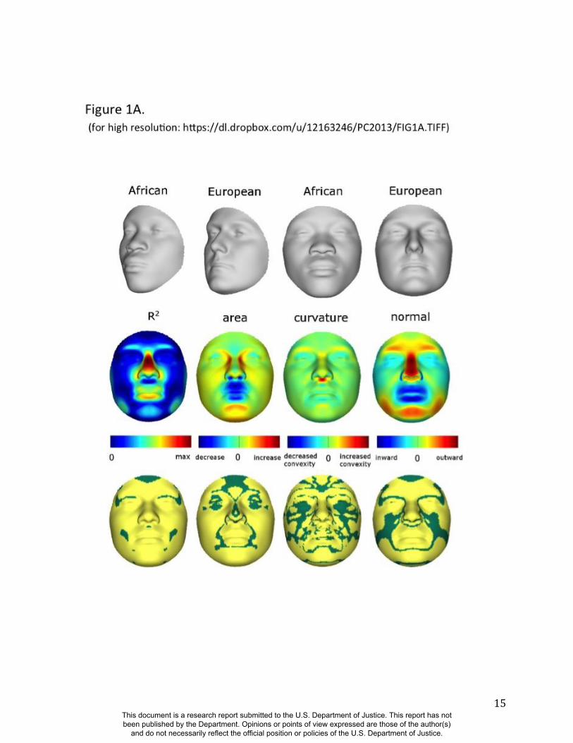
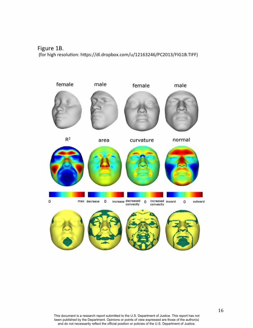
As expected, many parts of the face are affected by both ancestry and sex. Figure 1 illustrates the

partial effects of RIP-A and RIP-S on facial shape using transformations and heat maps for effect

size (R2) and the three primary FSCPs. Facial regions that are statistically significant for effect

size and the FSCPs are shown in Figures S37, S40, S41, and S42. The shape transformations

shown are set to the points three standard deviations plus and minus the mean RIP-A and RIP-S



6

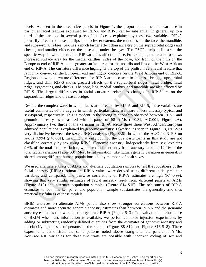
levels. As seen in the effect size panels in Figure 1, the proportion of the total variance in

particular facial features explained by RIP-A and RIP-S can be substantial. In general, up to a

third of the variance in several parts of the face is explained by these two variables. RIP-A

primarily affects the nose and lips and, to lesser extents, the roundness of the face, the mandible,

and supraorbital ridges. Sex has a much larger effect than ancestry on the supraorbital ridges and

cheeks, and smaller effects on the nose and under the eyes. The FSCPs help to illustrate the

specific ways in which particular RIP variables affect the face. For example, the area ratio shows

increased surface area for the medial canthus, sides of the nose, and front of the chin on the

European end of RIP-A and a greater surface area for the nostrils and lips on the West African

end of RIP-A. The curvature difference highlights the top of the philtrum as a facial feature that

is highly convex on the European end and highly concave on the West African end of RIP-A.

Regions showing curvature differences for RIP-A are also seen in the nasal bridge, supraorbital

ridges, and chin. RIP-S shows greatest effects on the supraorbital ridges, nasal bridge, nasal

ridge, zygomatics, and cheeks. The nose, lips, medial canthus, and mandible are also affected by

RIP-S. The largest differences in facial curvature related to changes in RIP-S are on the

supraorbital ridges and the nasal bridge.

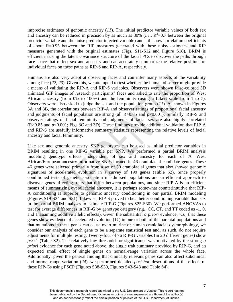
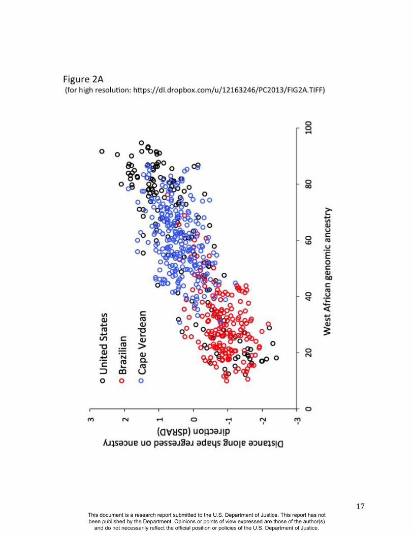
Despite the complex ways in which faces are affected by RIP-A and RIP-S, these variables are

useful summaries of the degree to which particular faces are more or less ancestry-typical and

sex-typical, respectively. This is evident in the strong relationship observed between RIP-A and

genomic ancestry as measured with a panel of 68 AIMs (r=0.81, p<0.001; Figure 2A).

Approximately two thirds of the variation in RIP-A across these three West African/European

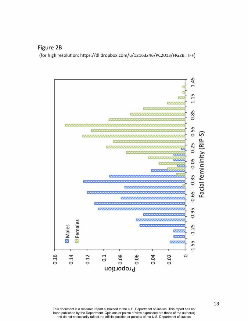
admixed populations is explained by genomic ancestry. Likewise, as seen in Figure 2B, RIP-S is

very distinctive between the sexes. ROC analyses (Fig. S36) show that the AUC for RIP-S on

sex is 0.994 (p<0.001), meaning that only four of the 592 participants in this study are not

classified correctly by sex using RIP-S. Genomic ancestry, independently from sex, explains

9.6% of the total facial variation, while sex independently from ancestry explains 12.9% of the

total facial variation (Table S3). Most facial variation, like human genetic variation in general, is

shared among different human populations and by members of both sexes.

We used alternate subsets of AIMs and alternate population samples to test the robustness of the

facial ancestry (RIP-A) estimation. RIP-A values were derived using different initial predictor

variables and compared. The pairwise correlations of RIP-A estimates are high (R2>0.99),

showing that very similar estimates of facial ancestry result from different panels of AIMs

(Figure S13) and alternate population samples (Figure S14-S15). The robustness of RIP-A

estimates to both marker panel and population sample substantiates the generality and thus

practical usefulness of these models.

BRIM analyses on alternate AIMs panels also show stronger correlations between RIP-A

estimates and more accurate genomic ancestry estimates than between RIP-A and the genomic

ancestry estimates that were used to generate RIP-A (Figure S13). To evaluate the performance

of BRIM when less information is available, we performed noise injection experiments by

adding or subtracting randomly defined quantities from the estimates of genomic ancestry and

misclassifying the sex of persons in the sample (Figure S8-S12 and Figure S16-S18). These

experiments demonstrate the same patterns noted above using alternate panels of AIMs:

Accurate RIP variables for these two traits are possible with incorrect coding of sex and



7

imprecise estimates of genomic ancestry (11). The initial predictor variable values of both sex

and ancestry can be reduced in precision by as much as 30% (i.e., R2=0.7 between the original

predictor variable and the noise predictor injected variable) and still show correlation coefficients

of about R=0.95 between the RIP measures generated with these noisy estimates and RIP

measures generated with the original estimates (Figs. S11-S12 and Figure S18). BRIM is

efficient in using the latent covariance structure of the facial PCs to discover the paths through

face space that reflect sex and ancestry and can accurately summarize the relative positions of

individual faces on these paths as RIP-S and RIP-A, respectively.

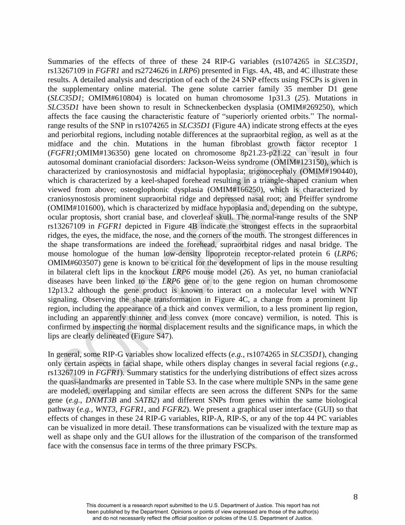
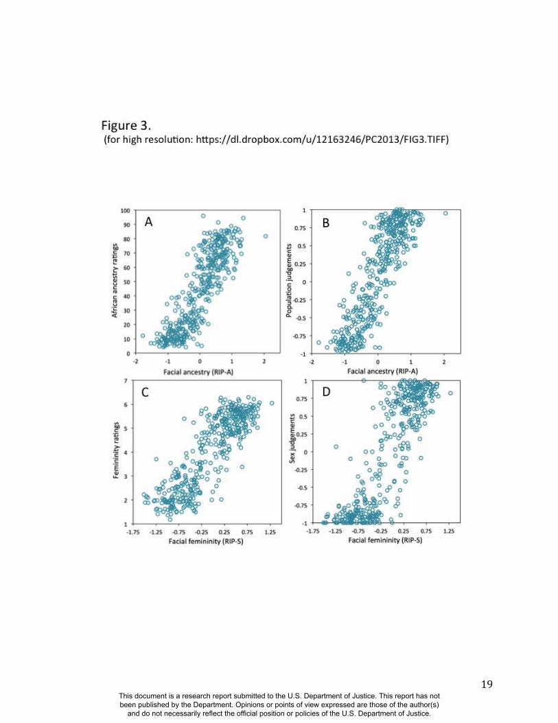
Humans are also very adept at observing faces and can infer many aspects of the variability

among face (22, 23). Given this, we attempted to test whether the human observer might provide

a means of validating the RIP-A and RIP-S variables. Observers were shown false-colored 3D

animated GIF images of research participants’ faces and asked to rate the proportion of West

African ancestry (from 0% to 100%) and the femininity (using a Likert scale from 1 to 7).

Observers were also asked to judge the sex and the population group (11). As shown in Figures

3A and 3B, the correlations between RIP-A and observer ratings of proportional facial ancestry

and judgments of facial population are strong (all R>0.85 and p<0.001). Similarly, RIP-S and

observer ratings of facial femininity and judgments of facial sex are also highly correlated

(R>0.85 and p<0.001; Figs 3C and 3D). These findings provide additional validation that RIP-A

and RIP-S are usefully informative summary statistics representing the relative levels of facial

ancestry and facial femininity.

Like sex and genomic ancestry, SNP genotypes can be used as initial predictor variables in

BRIM resulting in one RIP-G variable per SNP. We performed a partial BRIM analysis

modeling genotype effects independent of sex and ancestry for each of 76 West

African/European ancestry-informative SNPs located in 46 craniofacial candidate genes. These

46 genes were selected primarily from a set of 50 craniofacial genes that also showed genomic

signatures of accelerated evolution in a survey of 199 genes (Table S2). Since properly

conditioned tests of genetic association in admixed populations are an efficient approach to

discover genes affecting traits that differ between populations, and since RIP-A is an efficient

means of summarizing overall facial ancestry, it is perhaps somewhat counterintuitive that RIP-

A conditioning is superior to genomic ancestry conditioning in our partial BRIM modeling

(Figures S19-S24 and S31). Likewise, RIP-S proved to be a better conditioning variable than sex

in the partial BRIM analyses to estimate RIP-G (Figures S25-S30). We performed ANOVAs to

test for average differences in RIP-G by genotype category (e.g., CC, CT, and TT coded as -1, 0,

and 1 assuming additive allelic effects). Given the substantial a priori evidence, viz., that these

genes show evidence of accelerated evolution (11) in one or both of the parental populations and

that mutations in these genes can cause overt murine or human craniofacial dysmorphology, we

consider our analysis of each gene to be a separate statistical test and, as such, do not require

adjustments for multiple testing. Twenty-four of 76 RIP-G variables (in 20 different genes) show

p<0.1 (Table S2). The relatively low threshold for significance was motivated by the strong a

priori evidence for each gene noted above, the single trait summary provided by RIP-G, and an

expected small effect of single genes on normal-range variation across the whole face.

Additionally, given the general finding that clinically relevant genes can also affect subclinical

and normal-range variation (24), we performed detailed post hoc descriptions of the effects of

these RIP-Gs using FSCP (Figures S38-S39, Figures S43-S48 and Table S4).



8

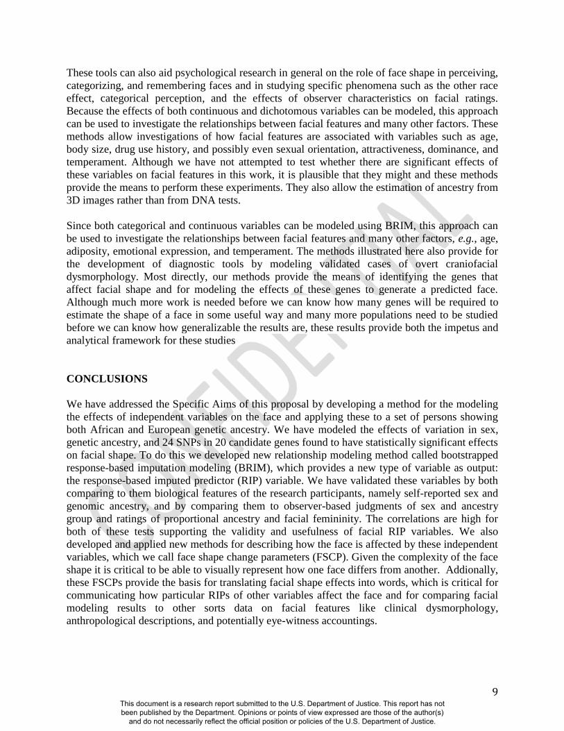
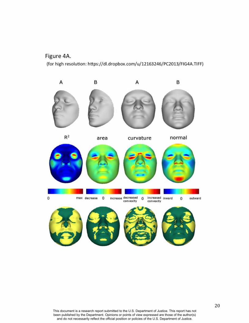
Summaries of the effects of three of these 24 RIP-G variables (rs1074265 in SLC35D1,

rs13267109 in FGFR1 and rs2724626 in LRP6) presented in Figs. 4A, 4B, and 4C illustrate these

results. A detailed analysis and description of each of the 24 SNP effects using FSCPs is given in

the supplementary online material. The gene solute carrier family 35 member D1 gene

(SLC35D1; OMIM#610804) is located on human chromosome 1p31.3 (25). Mutations in

SLC35D1 have been shown to result in Schneckenbecken dysplasia (OMIM#269250), which

affects the face causing the characteristic feature of “superiorly oriented orbits.” The normal-

range results of the SNP in rs1074265 in SLC35D1 (Figure 4A) indicate strong effects at the eyes

and periorbital regions, including notable differences at the supraorbital region, as well as at the

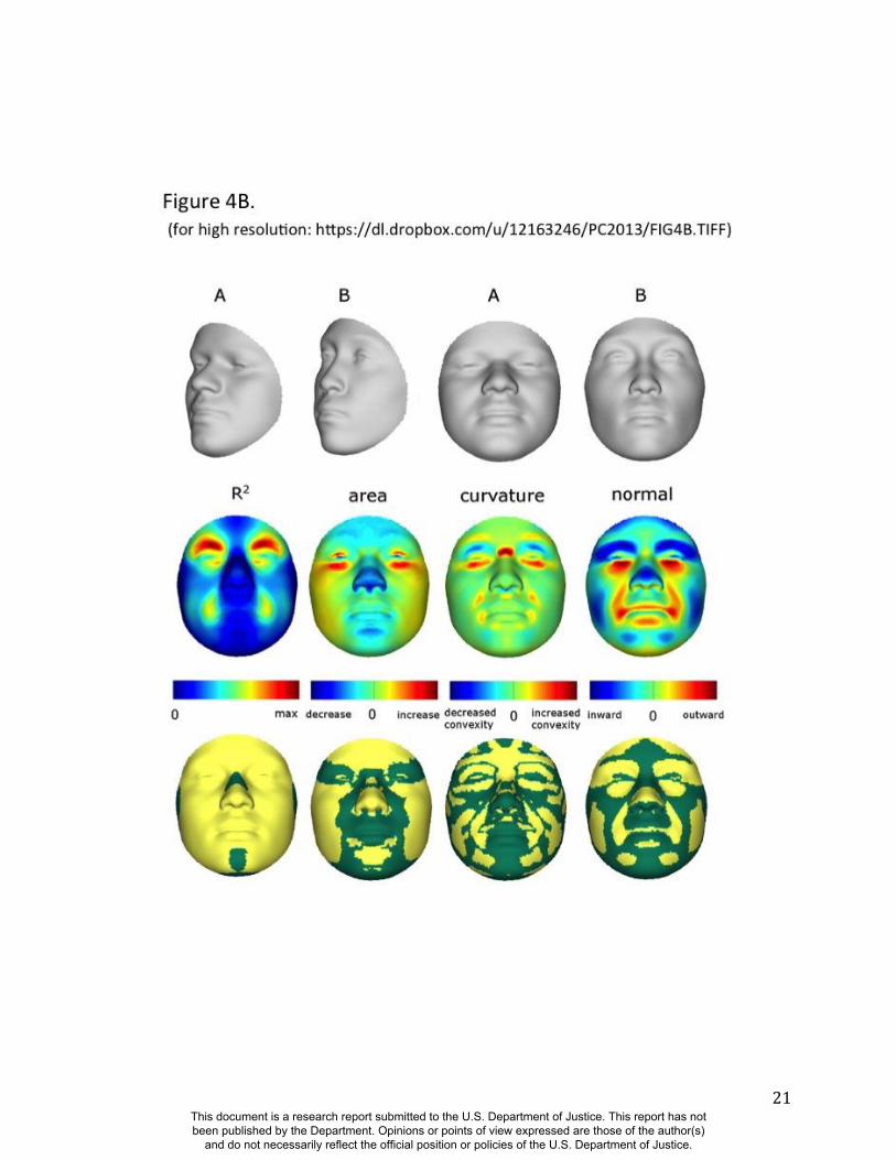
midface and the chin. Mutations in the human fibroblast growth factor receptor 1

(FGFR1;OMIM#136350) gene located on chromosome 8p21.23-p21.22 can result in four

autosomal dominant craniofacial disorders: Jackson-Weiss syndrome (OMIM#123150), which is

characterized by craniosynostosis and midfacial hypoplasia; trigonocephaly (OMIM#190440),

which is characterized by a keel-shaped forehead resulting in a triangle-shaped cranium when

viewed from above; osteoglophonic dysplasia (OMIM#166250), which is characterized by

craniosynostosis prominent supraorbital ridge and depressed nasal root; and Pfeiffer syndrome

(OMIM#101600), which is characterized by midface hypoplasia and, depending on the subtype,

ocular proptosis, short cranial base, and cloverleaf skull. The normal-range results of the SNP

rs13267109 in FGFR1 depicted in Figure 4B indicate the strongest effects in the supraorbital

ridges, the eyes, the midface, the nose, and the corners of the mouth. The strongest differences in

the shape transformations are indeed the forehead, supraorbital ridges and nasal bridge. The

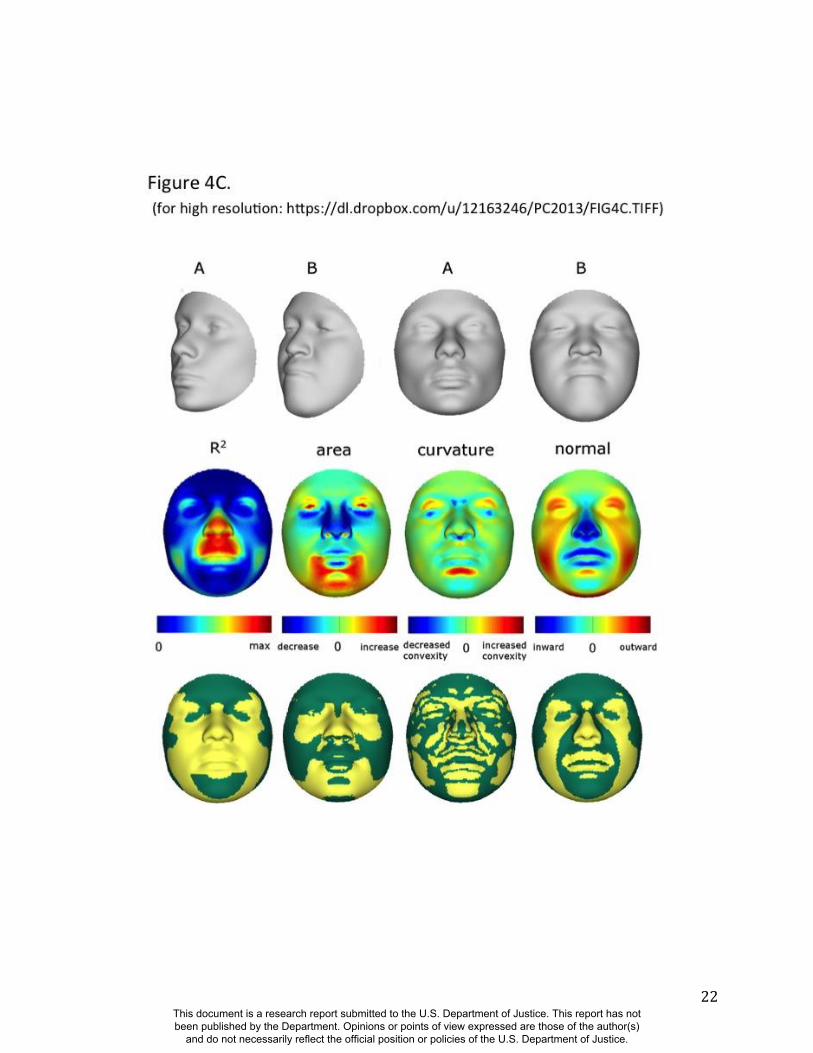
mouse homologue of the human low-density lipoprotein receptor-related protein 6 (LRP6;

OMIM#603507) gene is known to be critical for the development of lips in the mouse resulting

in bilateral cleft lips in the knockout LRP6 mouse model (26). As yet, no human craniofacial

diseases have been linked to the LRP6 gene or to the gene region on human chromosome

12p13.2 although the gene product is known to interact on a molecular level with WNT

signaling. Observing the shape transformation in Figure 4C, a change from a prominent lip

region, including the appearance of a thick and convex vermilion, to a less prominent lip region,

including an apparently thinner and less convex (more concave) vermilion, is noted. This is

confirmed by inspecting the normal displacement results and the significance maps, in which the

lips are clearly delineated (Figure S47).

In general, some RIP-G variables show localized effects (e.g., rs1074265 in SLC35D1), changing

only certain aspects in facial shape, while others display changes in several facial regions (e.g.,

rs13267109 in FGFR1). Summary statistics for the underlying distributions of effect sizes across

the quasi-landmarks are presented in Table S3. In the case where multiple SNPs in the same gene

are modeled, overlapping and similar effects are seen across the different SNPs for the same

gene (e.g., DNMT3B and SATB2) and different SNPs from genes within the same biological

pathway (e.g., WNT3, FGFR1, and FGFR2). We present a graphical user interface (GUI) so that

effects of changes in these 24 RIP-G variables, RIP-A, RIP-S, or any of the top 44 PC variables

can be visualized in more detail. These transformations can be visualized with the texture map as

well as shape only and the GUI allows for the illustration of the comparison of the transformed

face with the consensus face in terms of the three primary FSCPs.



9

These tools can also aid psychological research in general on the role of face shape in perceiving,

categorizing, and remembering faces and in studying specific phenomena such as the other race

effect, categorical perception, and the effects of observer characteristics on facial ratings.

Because the effects of both continuous and dichotomous variables can be modeled, this approach

can be used to investigate the relationships between facial features and many other factors. These

methods allow investigations of how facial features are associated with variables such as age,

body size, drug use history, and possibly even sexual orientation, attractiveness, dominance, and

temperament. Although we have not attempted to test whether there are significant effects of

these variables on facial features in this work, it is plausible that they might and these methods

provide the means to perform these experiments. They also allow the estimation of ancestry from

3D images rather than from DNA tests.

Since both categorical and continuous variables can be modeled using BRIM, this approach can

be used to investigate the relationships between facial features and many other factors, e.g., age,

adiposity, emotional expression, and temperament. The methods illustrated here also provide for

the development of diagnostic tools by modeling validated cases of overt craniofacial

dysmorphology. Most directly, our methods provide the means of identifying the genes that

affect facial shape and for modeling the effects of these genes to generate a predicted face.

Although much more work is needed before we can know how many genes will be required to

estimate the shape of a face in some useful way and many more populations need to be studied

before we can know how generalizable the results are, these results provide both the impetus and

analytical framework for these studies

CONCLUSIONS

We have addressed the Specific Aims of this proposal by developing a method for the modeling

the effects of independent variables on the face and applying these to a set of persons showing

both African and European genetic ancestry. We have modeled the effects of variation in sex,

genetic ancestry, and 24 SNPs in 20 candidate genes found to have statistically significant effects

on facial shape. To do this we developed new relationship modeling method called bootstrapped

response-based imputation modeling (BRIM), which provides a new type of variable as output:

the response-based imputed predictor (RIP) variable. We have validated these variables by both

comparing to them biological features of the research participants, namely self-reported sex and

genomic ancestry, and by comparing them to observer-based judgments of sex and ancestry

group and ratings of proportional ancestry and facial femininity. The correlations are high for

both of these tests supporting the validity and usefulness of facial RIP variables. We also

developed and applied new methods for describing how the face is affected by these independent

variables, which we call face shape change parameters (FSCP). Given the complexity of the face

shape it is critical to be able to visually represent how one face differs from another. Addionally,

these FSCPs provide the basis for translating facial shape effects into words, which is critical for

communicating how particular RIPs of other variables affect the face and for comparing facial

modeling results to other sorts data on facial features like clinical dysmorphology,

anthropological descriptions, and potentially eye-witness accountings.



10

We have recently compiled the bulk of our existing set of faces onto an initial World Face Space

(N=3,773 faces). This set of faces is primarily composed of persons for whom we also have

DNA, but also include a set of 3d photos of 27 life masks that were collected by anthropolgists in

the middle of the last century, which we photographed at the La Sapienza University

Anthropology museum in Rome, Italy. The preliminary analyses of this face space are quite

encouraging. For example, despite a four-fold difference if the number of faces between the two

face spaces, namely 592 vs 3,773 and the differences in the ancestry composition, West African

and European only vs. persons with Indigenous American, East Asian, South Asian, and four

different parts of Europe, the projected faces (namely those reconstructed from PC scores) for

the set of 592 that are in common between the two face spaces are strikingly similar. On visual

inspection, the faces reconstructed from the top PCs (those that explain 98% of the total

variation) are clearly identical. We also computed the procrustes difference, which is also known

as the root mean square error (RSME) and find that it is on average 0.003 between the two

projections a level that is about 1,000 times smaller than the average RMSE between to faces in

the original 592 face space. We are developing these analyses to more fully define this World

Face Space and will be investigating particular technical issues, such as at what point does the

face space become stable and whether constructing a face space without one or another group,

for example, leaving out men or women alternatively, compromises stability of the model. It is

notable that we can report the face space in a form that other researchers can use it without

necessarily including any of the individual PC scores for the individual faces that were used to

construct it. We will be adapting the interface for the DNA2FACEIN3D GUI that we are

providing to readers along-side the first paper, currently in review, to distribute with this World

Face Space, to provide various means of viewing and interacting with the face space. One such

extension is the ability of users to upload the PC scores of faces like, for example, predicted

faces that are made from compounding the effects of RIP variables into the space to enable the

visualization of particular faces. Users can also upload appropriately remapped face shapes and

derive the PC scores that explain the face in question. In this way, the RIP variables, like RIP-A,

can be estimated immediately from new faces without going through the rather computationally

intensive, especially at N=3,773 face, steps needed to compile the face space and run BRIM.

Future studies by our group will include an analysis of a set of 50,000 SNPs in a panel of 2,000

persons of African and European ancestry, which is underway in collaboration a small company

and a government contractor and partly funded by two DOD agencies. Some of the 50,000 SNPs

included on this chip include SNPs in tissue specific enhancers for human neural crest cell

(hNCC) lineage cells. These cells provide the developmental foundation for most of the

mammalian face and provide another important source of information for mapping the genes

affecting facial features. We have also initiated additional genotyping of subjects we have

already collected as well as sampling of new panels of subjects. One of these sampling events

will be taking place sometime in April 3013 which resulted in the collection of 117 persons each

of whom is getting their 23andMe test results (~$109 value including shipping) providing us

with both an attractive incentive for the recruitment of subjects as well as immediate access to

about 1,000,000 SNP genotypes. A very similar recruitment will start in mid-September 2013 on

the campus of the University of Texas at San Antonio is expected to result in a sample of 300

Mexican Americans. Given the mixed European and Indigenous American ancestry that

characterizes Mexican Americans, we expect this sample will contribute to our efforts to model

the effects of a new ancestry axis, complementing the West African/European axis described by



11

the RIP-A reported here. We also expect to be able to combine this sample with our existing

sample of ~800 Brazilians and ~100 other Latino research participants, many of whom also have

Indigenous American and European genomic ancestry in addition to varying levels of West

African ancestry. This World Face Space may also be useful in furthering biometric methods for

projecting 2d facial images into 3d space, a fundamental but difficult step is contemporary facial

biometric methods.

DISSEMINATION PLAN

We have submitted a manuscript based on these results to Science and were told by the editors

on June 28th

that it was being sent out for in-depth review. It is for this reason that we have

asked the NIJ program directors to not publish this Executive Summary or the Executive

Technical report until the primary article has been accepted for publication. If we do not

get favorable reviews from the editors and referees of Science, we will immediately submit it to

Nature Computational Biology and then to PLoS Genetics. Once the paper is in press, we will

contact the NIJ program directors and apprise them of the embargo date such that some of

all of this report could be released by NIJ. Again, we are requesting that the report not be

released until the embargo date. We are also in the process of preparing more technical papers

describing in greater detail the BRIM method and other results described herein. In addition to

print publications, we will also present these results in meetings like the American Association

of Physical Anthropologists, the Promega International Symposium on Human Identification

conference, and the American Society of Human Genetics, and will provide short science videos

describing the methods and results for various audiences. These videos will be posted on sites

like SciVee, YouTube, and Vimeo. Given the very visual nature of the human face and the

highly multidisciplinary way in which we are working, we feel these videos may help facilitate a

more rapid dissemination or our results.



12

GLOSSARY

Admixture mapping – the identification of genetic linkage relationships between markers and traits that differ between the parental populations. AIMs – ancestry informative markers – gene markers that show large differences in allele frequencies between two or more populations. Allele – alternate form of a genetic marker. In humans, SNPs usually have two alleles and STRs generally many more (between 10 and 20). Functional alleles are variants that directly affect the phenotypic expression of a particular trait or disease risk. AUC – area under the curve – the primary statistic in Reporter Opperatin Characteristic (ROC) analysis. It is a measure of the ability of the data to correctly classify a bivariate trait. Biometrics – the process of comparing physical measures to one another to discover or verify identity. Bootstrap – the process of iteratively running a procedure where the results of one run are the input values for the next. Candidate genes – genes suspected of playing a role in a trait or disease process from biochemical or other types of information. BRIM – bootstrapped response-based imputation modeling – an iterative statistical method for modeling relationships between predictor and response variables. FSCP – facial shape change parameters – means to describe the shape differences between two faces. Gene – a functional segment of DNA. Genes can be protein-coding sequences, sequences that are functional when transcribed into RNA, or those that are biologically functional as DNA. Genotype – the combination of alleles at an autosomal locus that a person inherits from his mother and father. hNCC – human Neural Crest Cells – Cells of developmental lineage known as the neural crest that forms early in embryogenesis. These cells migrate throughout the body becoming melanocyte, forming much of the face among other tissues. Imputation – the process of estimating a missing value from the bulk of the rest of the data. The usage of imputation in BRIM is unique in that each observation in turn is purposefully made missing and its values imputed. Locus – (plural = loci) – a particular position in the genome. Molecular photofitting – the process of predicting a forensically useful superficial trait value from genetic markers. Indirect molecular photofitting is when the trait values are estimated from AIMs and direct molecular photofitting is when estimates are also based on the genotypes of functional markers. Morphometrics – quantitative analysis of form, a concept that encompasses size and shape. PLS - partial least squares – a form of relationship modeling in which the response variable space as well as the predictor variable space can be multivariate. Population stratification – the result of non-random mating among individuals in a sample that can result from either reproductive isolation in a resident population or the combination of more than one randomly mating population.



13

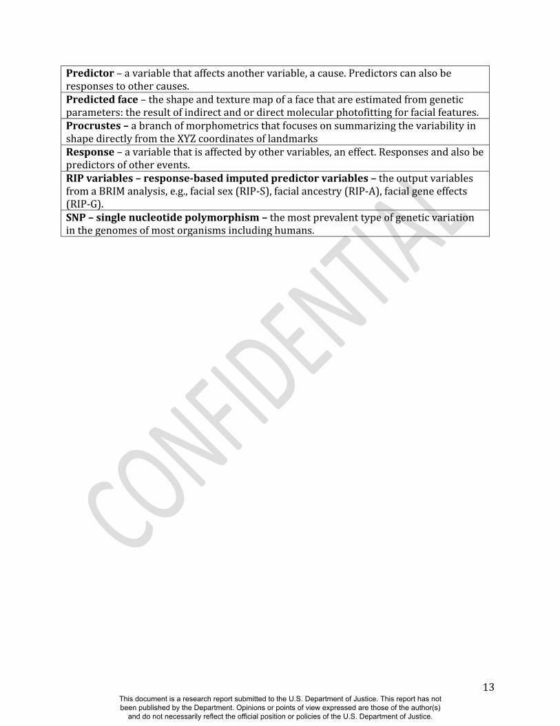
Predictor – a variable that affects another variable, a cause. Predictors can also be responses to other causes. Predicted face – the shape and texture map of a face that are estimated from genetic parameters: the result of indirect and or direct molecular photofitting for facial features. Procrustes – a branch of morphometrics that focuses on summarizing the variability in shape directly from the XYZ coordinates of landmarks Response – a variable that is affected by other variables, an effect. Responses and also be predictors of other events. RIP variables – response-based imputed predictor variables – the output variables from a BRIM analysis, e.g., facial sex (RIP-S), facial ancestry (RIP-A), facial gene effects (RIP-G). SNP – single nucleotide polymorphism – the most prevalent type of genetic variation in the genomes of most organisms including humans.



14

TABLES and FIGURE LEGENDS

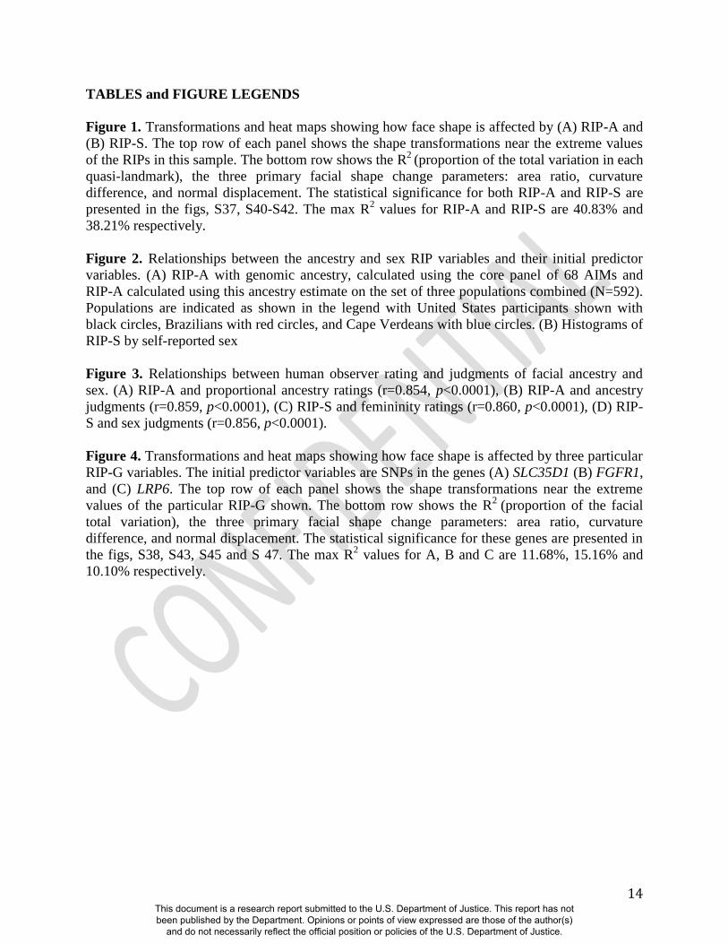
Figure 1. Transformations and heat maps showing how face shape is affected by (A) RIP-A and

(B) RIP-S. The top row of each panel shows the shape transformations near the extreme values

of the RIPs in this sample. The bottom row shows the R2

(proportion of the total variation in each

quasi-landmark), the three primary facial shape change parameters: area ratio, curvature

difference, and normal displacement. The statistical significance for both RIP-A and RIP-S are

presented in the figs, S37, S40-S42. The max R2 values for RIP-A and RIP-S are 40.83% and

38.21% respectively.

Figure 2. Relationships between the ancestry and sex RIP variables and their initial predictor

variables. (A) RIP-A with genomic ancestry, calculated using the core panel of 68 AIMs and

RIP-A calculated using this ancestry estimate on the set of three populations combined (N=592).

Populations are indicated as shown in the legend with United States participants shown with

black circles, Brazilians with red circles, and Cape Verdeans with blue circles. (B) Histograms of

RIP-S by self-reported sex

Figure 3. Relationships between human observer rating and judgments of facial ancestry and

sex. (A) RIP-A and proportional ancestry ratings (r=0.854, p<0.0001), (B) RIP-A and ancestry

judgments (r=0.859, p<0.0001), (C) RIP-S and femininity ratings (r=0.860, p<0.0001), (D) RIP-

S and sex judgments (r=0.856, p<0.0001).

Figure 4. Transformations and heat maps showing how face shape is affected by three particular

RIP-G variables. The initial predictor variables are SNPs in the genes (A) SLC35D1 (B) FGFR1,

and (C) LRP6. The top row of each panel shows the shape transformations near the extreme

values of the particular RIP-G shown. The bottom row shows the R2

(proportion of the facial

total variation), the three primary facial shape change parameters: area ratio, curvature

difference, and normal displacement. The statistical significance for these genes are presented in

the figs, S38, S43, S45 and S 47. The max R2 values for A, B and C are 11.68%, 15.16% and

10.10% respectively.



15



16



17



18



19



20



21



22



23

TECHNICALLY DETAILED MATERIALS AND METHODS

1 Samples and DNA collection Population samples were collected in the United States (State College, PA, Williamsport, PA,

and The Bronx, NY); Brasilia, Brazil; and Cape Verde (São Vicente, and Santiago), all under a

Penn State University Internal Review Board (IRB) approved research protocol titled, “Genetics

of Human Pigmentation, Ancestry and Facial Features.” Skin pigmentation was measured using

narrow-band reflectometry with the DermaSpectrometer (Cortrex Technology, Hadsund,

Denmark) in the United States and Brazil and the DSMII (Cortrex Technology, Hadsund,

Denmark) in Cape Verde. DermaSpectrometer readings were rescaled to the DSMII scale by

multiplying by 1.19, the slope derived from a comparison of readings with both instruments on

the same set of participants (data not shown). Height, weight, age, self-reported ancestry, and sex

were collected by survey. DNA was collected both with buccal cell brushes and using finger-

stick blood on four-circle Whatman FTA cards (Whatman, Florham Park, NJ).

To minimize age-related variation in facial morphology, we only recruited participants between

the ages of 18 and 40. From these recruits, we selected individuals with >10% West African

ancestry and <15% combined Native American and East-Asian ancestry as measured with the

176 ancestry informative marker (AIM) panel. We assigned these cutoff points to reduce

admixture from parental populations other than West African and European. Ancestry-based

exclusion criteria were not applied to Cape Verdeans given the largely dihybrid nature of this

population. Finally, we excluded participants whose 3D images were obstructed by facial or head

hair. After excluding participants by these criteria, we were left with 592 participants (154 from

the US, 191 from Brazil, and 247 from Cape Verde).

2 Genotyping and ancestry estimates

Genotyping of 176 AIMs for the US and Brazilian samples was performed on the 25 K

SNPstream ultra-high-throughput genotyping system (Beckman Coulter, Fullerton, CA) as

previously described (12). Ancestry was estimated using the various panels of AIMs by one of

two methods. Ancestry using full set of 176 AIMs was estimated in the US and Brazilian

subsample using maximum likelihood on a four-population model; European, West African,

Native American, and East Asian (12).The 68-AIM ancestry estimates were generated using the

full sample (U.S., Brazilian, and Cape Verdean) using ADMIXMAP as these markers were

available on all 592 participants. One marker (rs917502) from the original 176 had a call rate of

less than 30% and was omitted from the ADMIXMAP analyses.

The Cape Verdean sample was assayed for the Illumina Infinium HD Human1M-Duo Beadarray

(Illumina, San Diego, CA) following the manufacturer’s recommendations. A total of 537,895

autosomal SNPs that passed quality controls were used to estimate ancestry using the program

FRAPPE (27), assuming two ancestral populations (West African and European). HapMap

genotype data, including 60 unrelated European-Americans (CEU) and 60 unrelated West

Africans (YRI), were incorporated in the analysis as reference panels (phase 2, release 22, The

HapMap Project; 28).



24

We identified a list of selection-nominated candidate genes for testing against normal-range

facial variation in admixed individuals of European and West African descent. Ancestry

information and tests for accelerated evolution (29)were used to prioritize among a larger set of

craniofacial genes. Since most genomic regions show low levels of allele frequency change

across human populations, genes affecting traits that vary across populations are usually

distinctive in showing large differences in frequency and other features of local variation and

allele frequency spectra consistent with rapid local evolution. A preliminary set of craniofacial

candidate genes was developed by searching the Online Mendelian Inheritance in Man (OMIM)

database (25). The keywords “craniofacial” and “facial” were searched to determine a set of

genes known to affect craniofacial development. The OMIM entries for each gene included in

the search output were then scanned manually to remove genes where the term appeared as a

result of phrases such as “no craniofacial associations found” and other similar negative results.

OMIM searching resulted in a list of 199 unique craniofacial candidate genes. Because this work

focused on admixed populations of West African and European descent, the statistical power to

detect linkage with craniofacial variation is greatest for SNPs that show large allele frequency

differences between West African and European parental populations. Therefore, allele

frequency differences among parental groups were further used to prioritize among the candidate

genes. SNP frequency data in putative parental population (CEPH Europeans (CEU) and

Yoruban (YRI) West Africans) for all SNPs within the 199 OMIM candidate genes were pulled

from the HapMap database. This reduced subset of genes was then tested for signatures of

natural selection in a 200 kb window surrounding each gene using a combination of three

statistical tests: Locus-Specific Branch Length (LSBL) (30), the log of the ratio of the

heterozygosities (lnRH) (31), and Tajima’s D (32). Because these tests are inferring different

concepts regarding population history, we considered as significant any gene with statistical

evidence of selection for all three measures or strong evidence of natural selection for two

measures in either West African and/or European parental populations as a Selection-Nominated

Candidate Gene (SNCG). A total of 50 autosomal genes were selected as SNCGs (SKI, LMNA,

SIL1, EDN1, RSPO2, TRPS1, POLR1D, MAP2K1, ADAMTS10, TBX1, PEX14, HSPG2, CAV3,

CTNND2, TFAP2A, PEX6, PEX3, MEOX2, RELN, ROR2, NEBL, CHUK, FGFR2, WT1, PEX16,

BMP4, FANCA, RAI1, FOXA2, ECE1, DPYD, ZEB2, SATB2, FGFR3, NIPBL, NSD1, ENPP1,

GLI3, COL1A2, BRAF, ASPH, FREM2, SNRPN, FBN1, MAP2K2, RPS19, DNMT3B, GDF5, and

UFD1L) and a set of SNPs with high allele frequency differences (delta > 0.4) in these 50

craniofacial Selection Nominated Candidate Genes to test for associations with facial shape

variation.

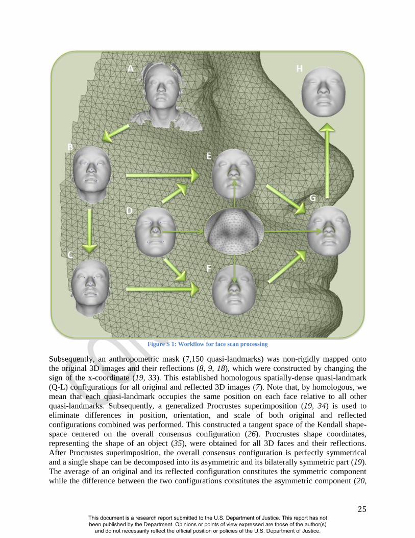
3 3D Facial Images and Phenotyping

3D images composed of surface and texture maps were taken using the 3dMDface system

(3dMD, Atlanta, GA). Participants were asked to close their mouths and hold their faces with a

neutral expression for the picture. Images were then exported from the 3dMD Patient software in

OBJ file format and imported into a scan cleaning program for cropping and trimming, removing

hair, ears, and any dissociated polygons. The complete work flow involved in processing face

scans is depicted in Figure S 1. Five positioning landmarks were placed on the face to establish a

rough facial orientation.



25

Figure S 1: Workflow for face scan processing

Subsequently, an anthropometric mask (7,150 quasi-landmarks) was non-rigidly mapped onto

the original 3D images and their reflections (8, 9, 18), which were constructed by changing the

sign of the x-coordinate (19, 33). This established homologous spatially-dense quasi-landmark

(Q-L) configurations for all original and reflected 3D images (7). Note that, by homologous, we

mean that each quasi-landmark occupies the same position on each face relative to all other

quasi-landmarks. Subsequently, a generalized Procrustes superimposition (19, 34) is used to

eliminate differences in position, orientation, and scale of both original and reflected

configurations combined was performed. This constructed a tangent space of the Kendall shape-

space centered on the overall consensus configuration (26). Procrustes shape coordinates,

representing the shape of an object (35), were obtained for all 3D faces and their reflections.

After Procrustes superimposition, the overall consensus configuration is perfectly symmetrical

and a single shape can be decomposed into its asymmetric and its bilaterally symmetric part (19).

The average of an original and its reflected configuration constitutes the symmetric component

while the difference between the two configurations constitutes the asymmetric component (20,



26

36). The analyses in this report were all based on facial shape as represented using the

component of symmetry only, as deviations from bilateral symmetry are thought to be the effects

of developmental noise and/or environmental factors rather than genes (37)

Principal components analysis (PCA) (10) on the superimposed and symmetrized quasi-

landmark configurations of the panel of 592 participants resulted in 44 PCs that together

summarize 98% of the total variation in face space. To examine the effect of excluding lower

PCs we first reconstructed actual quasi-landmark configuration from the 44 PCs only and

compared these to the original remapped face. We found that the average root mean squared

error (RMSE) is as small as 0.2 mm per quasi-landmark. The localized differences between the

original faces and the faces as represented by the first 44 PCs are largest around the iris, eyelids,

under the nose, and the corners and opening of the mouth and are at most about 0.45 mm. How a

PC or any other independent variable affects the face can be shown with heat maps and shape

transformations: heat maps use contrasting colors to highlight the specific parts of the face that

are affected while shape transformations illustrate the changes in overall face shape with two or

more images of the face at set intervals. Shape transformations are obtained from the average

face in the direction of each PC at -3 and +3 times the accompanying standard deviation (square-

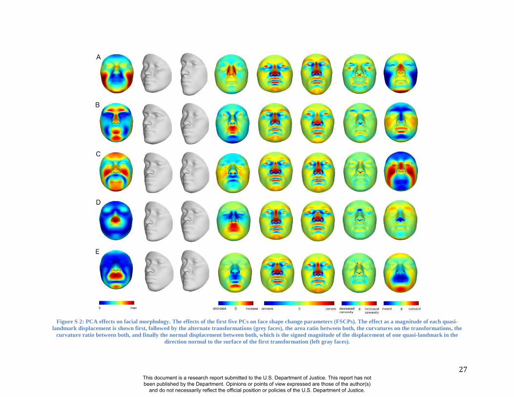
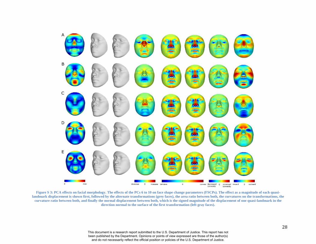
root of the eigenvalue). Figure S 2 and Figure S 3 show how the first 10 PCs affect the face.

Some of these PCs (e.g., PC1, PC2, PC3) summarize effects on many parts of the face, while

other PCs (e.g., PC4, PC5) summarize the effects of changes in only particular parts of the face.

The effects of each of the 44 PCs as well as the RIP variables can be visualized in using a GUI

software tool that we have written called DNA2FACEIN3D.EXE. The program and instruction

manual can be downloaded here:

https://dl.dropboxusercontent.com/u/12163246/PC2013/DNA2FACEIN3D.zip

We have used three methods to visualize and quantify facial difference so that we can

systematically express the effects of particular response-based imputed predictor (RIP) variables

on the face into anatomically interpretable results. These are based on comparing faces pairwise,

like the most feminine RIP-S to the most masculine RIP-S variables on the consensus face using

three fundamental measures: area ratio, normal displacement, and curvature ratio. These two

ratios and one displacement along with particular inter-landmark distances and angles can

together be termed face shape change parameters (FSCPs) and are a means of translating face

shape changes from the abstract face space into language of facial characteristics such that

comparisons between clinical or anthropological descriptions of faces can be compared to

bootstrapped response-based imputation modeling (BRIM) results. The statistical significance of

these FSCPs can be estimated using permutation. A more detailed description on how this is

done is given in section 5.4.



27

Figure S 2: PCA effects on facial morphology. The effects of the first five PCs on face shape change parameters (FSCPs). The effect as a magnitude of each quasi-

landmark displacement is shown first, followed by the alternate transformations (grey faces), the area ratio between both, the curvatures on the transformations, the

curvature ratio between both, and finally the normal displacement between both, which is the signed magnitude of the displacement of one quasi-landmark in the

direction normal to the surface of the first transformation (left gray faces).



28

Figure S 3: PCA effects on facial morphology. The effects of the PCs 6 to 10 on face shape change parameters (FSCPs). The effect as a magnitude of each quasi-

landmark displacement is shown first, followed by the alternate transformations (grey faces), the area ratio between both, the curvatures on the transformations, the

curvature ratio between both, and finally the normal displacement between both, which is the signed magnitude of the displacement of one quasi-landmark in the

direction normal to the surface of the first transformation (left gray faces).



29

4 Human observer ratings and judgments

4.1 Ancestry and Sex Observations:

Given the dexterity humans have for discerning numerous traits, features, and expressions,

it’s reasonable to expect the observer would provide a useful reference point for studies of

the genetics of facial traits. We accessed observer ratings and judgments of sex and

ancestry in order to test the informativeness of RIP-A and RIP-S. Selection of Stimuli: A total of 500 participant faces were selected and divided into twenty-five

panels of twenty faces, with each panel including faces of research participants across the range

of genomic ancestry levels and similar numbers of male and female faces. We used false colored

grey GIF animations so that ancestry and sex ratings and judgments would be based on face-

shape cues but not cues of skin, iris, or hair pigmentation or hair texture. Animation order was

randomized.

Administration of Instruments: We administered the instruments containing the animated, false-

colored GIFs with accompanying questions using Survey Monkey (SurveyMonkey.com LLC;

Palo Alto, CA). Four survey questions were relevant to this study:

1. “What proportion (from 0% to 100%) of this person’s ancestry appears to be West

African?” (Ratings made with a number between 0 and 100.)

2. Which single categorical group best describes this person? (Judged with Black

African, or African-American; White, European or European-American; or Mixed)

3. Does this person appear to be male or female? (Judged with “male” or “female”)

4. “How feminine does this person’s face appear to you?” (Ratings made with a choice

from a 7-point Likert scale ranging from 1 “extremely feminine” to 7 “extremely

masculine”.)

Observers were randomly assigned to one of the 25 panels through a link on the Anthropology

Department homepage.

Recruitment of Observers (PSU): Observers were recruited from students enrolled at Penn State

University. Of the 822 participants, 711 completed the surveys. The number of observers for the

ten alternative surveys ranged from 53 to 92, with a mean of 71. Observers who completed fewer

than half of the survey as well as three whose discrepancies were more than three standard

deviations from the mean were excluded from the analysis.

Recruitment of Observers (UCONN): Observers were recruited from students enrolled at the

University of Connecticut. A total of 139 completed the survey. The number of observers for

each of the three instruments ranged from 35 to 46, with a mean of 45. Observers completing

fewer than half of the survey as well as four whose discrepancies were more than three standard

deviations from the mean were excluded from the analysis.



30

5 Bootstrapped response-based imputation modeling (BRIM)

5.1 Regression Analysis

Ordinary regression (38)only assumes or allows errors in the response variable(s) and will be

detrimentally influenced by inaccurate predictor variables, lowering the stability, efficiency, and

statistical power. More advanced regression models, such as, partial least squares regression

(PLSR) (39, 40), allow imprecision in predictors as well as in responses. It is the case with all

regression methods that high levels of error in the predictors reduce the statistical power of the

association testing and lowering predictive power. We developed a bootstrapped response-based

imputation modeling (BRIM) technique to overcome the limitations of traditional relationship

modeling methods. BRIM, an extension of current regression techniques, uses response variables

to refine, filter, and transform one or more predictor variables. The output of BRIM is a new type

of variable: the response-based imputed predictor (RIP) variable. This is a hybrid or bridging

variable that combines information from both the predictor and response variables, creating a

novel variable space. From the point-of-view of the response variable, the RIP variable is a

supervised recoding of a multivariate response variable into a simpler univariate variable. Thus,

the RIP variable can be used to test associations against the predictors and can also be used to

visualize the predictor effects on the multivariate-response. From the point-of-view of the

predictor, the RIP is a response-based transformation of a likely less precise predictor variable

that recovers response-specific information and allows, for example, the transformation of

discretely coded (categorical) predictors into continuously distributed RIP variables.

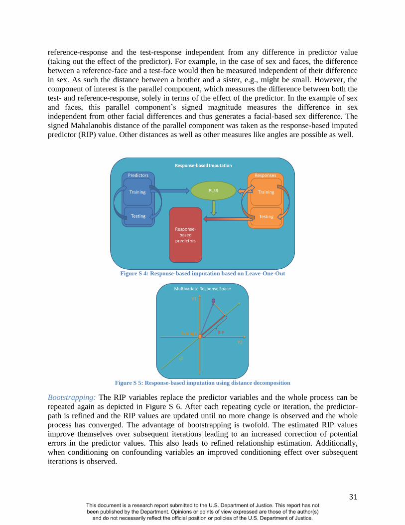
5.2 Generating RIP variables

Assume a set of observations { } comprising a set of predictor values

{ } and a set of response values {

} . Without loss of generality, we assume a linear Partial Least Squares Regression

(PLSR) model . Here , is the relationship between and Based on a “leave-N-out”

(LNO) approach the set of observations is divided into a training set and a test set as

illustrated in Figure S 4. In this work, a leave-one-out (LOO) scheme was applied: each

observation is removed, in turn, from the set of observations and used as a test case, while the

rest are used as training cases. The training set of observations is used to learn the PLSR

model and to establish the relationship . For every predictor in this relationship a “path is

drawn” or a direction is established in the response-space, which explains the variation in the

responses caused by the particular predictor, which is known as the regression line and referred

to as a predictor-path. This concept is illustrated in Figure S 5. Moving along such a path will

change the response values in function of a particular predictor value. For example, if the

predictor is sex and the response is facial morphology, moving along such a sex-path will casue

the face to change from male to female and vice-versa.

For all the observations in the test set , a response-based predictor value is imputed as

follows: first a point of reference or a reference-response on the predictor-path is chosen, for

which we took the point of origin in the response-space after centering all the response variables.

Subsequently, in a multivariate case, the vector of a test-response to this reference-response is

decomposed into a component perpendicular and a component parallel to the predictor-path. The

component perpendicular to the path is known as the response-residual. Because of the

perpendicular nature the magnitude of this component, measures the difference between the



31

reference-response and the test-response independent from any difference in predictor value

(taking out the effect of the predictor). For example, in the case of sex and faces, the difference

between a reference-face and a test-face would then be measured independent of their difference

in sex. As such the distance between a brother and a sister, e.g., might be small. However, the

component of interest is the parallel component, which measures the difference between both the

test- and reference-response, solely in terms of the effect of the predictor. In the example of sex

and faces, this parallel component’s signed magnitude measures the difference in sex

independent from other facial differences and thus generates a facial-based sex difference. The

signed Mahalanobis distance of the parallel component was taken as the response-based imputed

predictor (RIP) value. Other distances as well as other measures like angles are possible as well.

Figure S 4: Response-based imputation based on Leave-One-Out

Figure S 5: Response-based imputation using distance decomposition

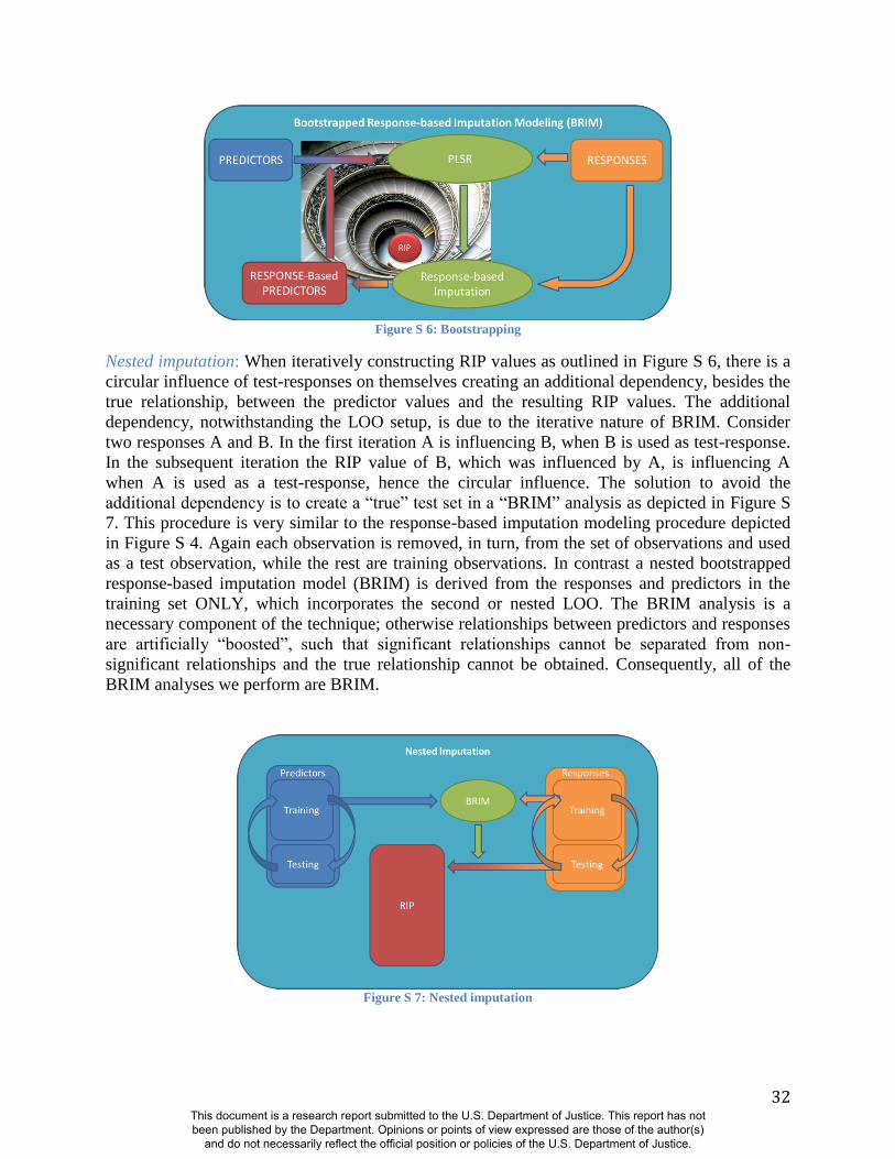
Bootstrapping: The RIP variables replace the predictor variables and the whole process can be

repeated again as depicted in Figure S 6. After each repeating cycle or iteration, the predictor-

path is refined and the RIP values are updated until no more change is observed and the whole

process has converged. The advantage of bootstrapping is twofold. The estimated RIP values

improve themselves over subsequent iterations leading to an increased correction of potential

errors in the predictor values. This also leads to refined relationship estimation. Additionally,

when conditioning on confounding variables an improved conditioning effect over subsequent

iterations is observed.



32

Figure S 6: Bootstrapping

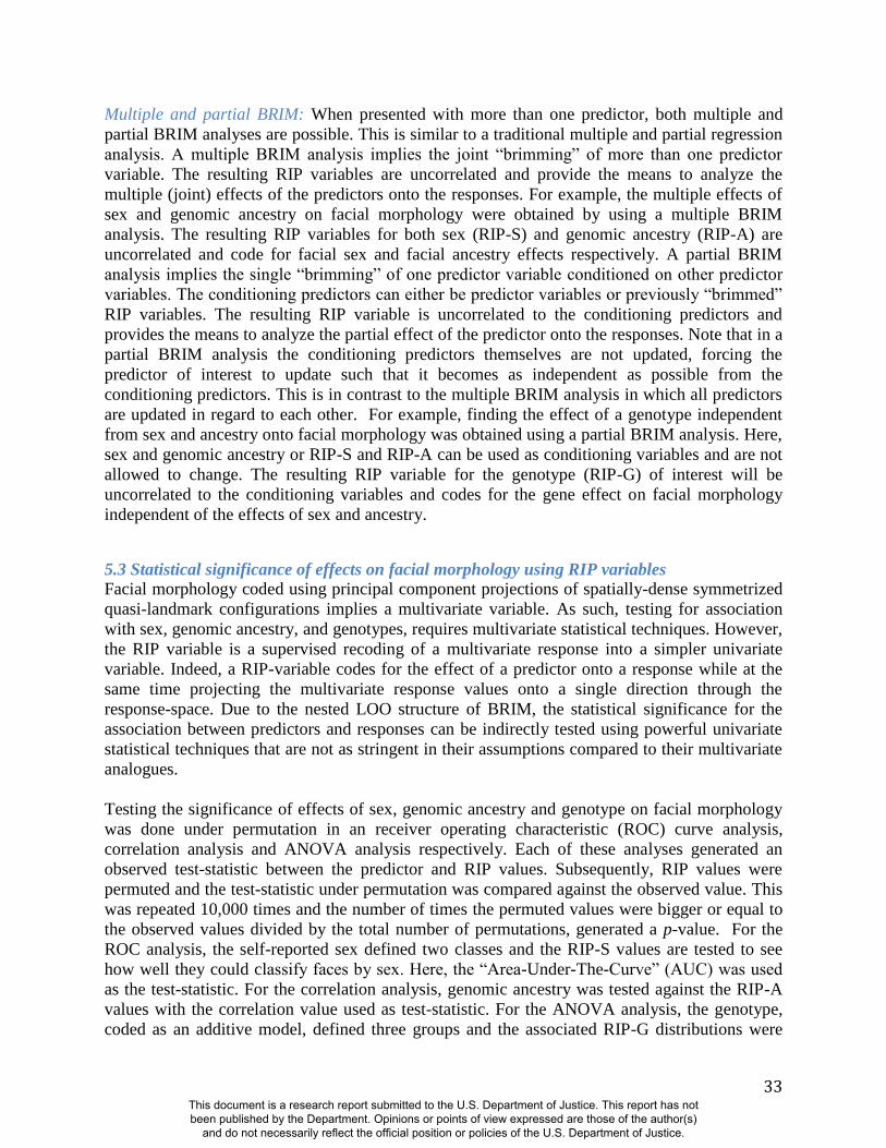
Nested imputation: When iteratively constructing RIP values as outlined in Figure S 6, there is a

circular influence of test-responses on themselves creating an additional dependency, besides the

true relationship, between the predictor values and the resulting RIP values. The additional

dependency, notwithstanding the LOO setup, is due to the iterative nature of BRIM. Consider

two responses A and B. In the first iteration A is influencing B, when B is used as test-response.

In the subsequent iteration the RIP value of B, which was influenced by A, is influencing A

when A is used as a test-response, hence the circular influence. The solution to avoid the

additional dependency is to create a “true” test set in a “BRIM” analysis as depicted in Figure S

7. This procedure is very similar to the response-based imputation modeling procedure depicted

in Figure S 4. Again each observation is removed, in turn, from the set of observations and used

as a test observation, while the rest are training observations. In contrast a nested bootstrapped

response-based imputation model (BRIM) is derived from the responses and predictors in the

training set ONLY, which incorporates the second or nested LOO. The BRIM analysis is a

necessary component of the technique; otherwise relationships between predictors and responses

are artificially “boosted”, such that significant relationships cannot be separated from non-

significant relationships and the true relationship cannot be obtained. Consequently, all of the

BRIM analyses we perform are BRIM.

Figure S 7: Nested imputation



33

Multiple and partial BRIM: When presented with more than one predictor, both multiple and

partial BRIM analyses are possible. This is similar to a traditional multiple and partial regression

analysis. A multiple BRIM analysis implies the joint “brimming” of more than one predictor

variable. The resulting RIP variables are uncorrelated and provide the means to analyze the

multiple (joint) effects of the predictors onto the responses. For example, the multiple effects of

sex and genomic ancestry on facial morphology were obtained by using a multiple BRIM

analysis. The resulting RIP variables for both sex (RIP-S) and genomic ancestry (RIP-A) are

uncorrelated and code for facial sex and facial ancestry effects respectively. A partial BRIM

analysis implies the single “brimming” of one predictor variable conditioned on other predictor

variables. The conditioning predictors can either be predictor variables or previously “brimmed”

RIP variables. The resulting RIP variable is uncorrelated to the conditioning predictors and

provides the means to analyze the partial effect of the predictor onto the responses. Note that in a

partial BRIM analysis the conditioning predictors themselves are not updated, forcing the

predictor of interest to update such that it becomes as independent as possible from the

conditioning predictors. This is in contrast to the multiple BRIM analysis in which all predictors

are updated in regard to each other. For example, finding the effect of a genotype independent

from sex and ancestry onto facial morphology was obtained using a partial BRIM analysis. Here,

sex and genomic ancestry or RIP-S and RIP-A can be used as conditioning variables and are not

allowed to change. The resulting RIP variable for the genotype (RIP-G) of interest will be

uncorrelated to the conditioning variables and codes for the gene effect on facial morphology

independent of the effects of sex and ancestry.

5.3 Statistical significance of effects on facial morphology using RIP variables

Facial morphology coded using principal component projections of spatially-dense symmetrized

quasi-landmark configurations implies a multivariate variable. As such, testing for association

with sex, genomic ancestry, and genotypes, requires multivariate statistical techniques. However,

the RIP variable is a supervised recoding of a multivariate response into a simpler univariate

variable. Indeed, a RIP-variable codes for the effect of a predictor onto a response while at the

same time projecting the multivariate response values onto a single direction through the

response-space. Due to the nested LOO structure of BRIM, the statistical significance for the

association between predictors and responses can be indirectly tested using powerful univariate

statistical techniques that are not as stringent in their assumptions compared to their multivariate

analogues.

Testing the significance of effects of sex, genomic ancestry and genotype on facial morphology

was done under permutation in an receiver operating characteristic (ROC) curve analysis,

correlation analysis and ANOVA analysis respectively. Each of these analyses generated an

observed test-statistic between the predictor and RIP values. Subsequently, RIP values were

permuted and the test-statistic under permutation was compared against the observed value. This

was repeated 10,000 times and the number of times the permuted values were bigger or equal to

the observed values divided by the total number of permutations, generated a p-value. For the

ROC analysis, the self-reported sex defined two classes and the RIP-S values are tested to see

how well they could classify faces by sex. Here, the “Area-Under-The-Curve” (AUC) was used

as the test-statistic. For the correlation analysis, genomic ancestry was tested against the RIP-A

values with the correlation value used as test-statistic. For the ANOVA analysis, the genotype,

coded as an additive model, defined three groups and the associated RIP-G distributions were



34

tested for different means where the F-statistic was used as test-statistic. Additionally, pair-wise

ANOVA analyses between all three groups were performed in a similar way.

5.4 Visualizing and analyzing effects on facial morphology using RIP variables

Effect and effect-size analysis: Principal components analysis on the 7,150 quasi-landmarks

coordinates across the set of 592 research participants results in a series of orthogonal PCs. The

first 44 PCs explain 98% of the total facial variation in this set of faces. These 44 PCs are the

responses variable matrix used to compute the RIP variables for sex, ancestry, and genotype. To

visualize and analyze their effect on facial morphology, first quasi-landmark configurations of

faces are reconstructed from the 44 PCs. Subsequently; these are directly regressed on the RIP

variables using PLSR. The effect on a particular quasi-landmark is then measured as the

magnitude or Euclidean distance of its displacement in 3D space. The effect-size or strength of

the relationship is reported as the variance explained by the PLSR model (R2). The partial effects

(one variable independent from the others in a multiple regression) are coded in the partial

regression coefficients. The partial effect-sizes are reported as the partial R2

values obtained from

a reduced regression model. This reduced model is the regression model for a single independent

variable after statistically removing the effect of all the other independent variables onto both the

single independent variable itself and the dependent variable (40). Statistical significance of both

multiple and partial effects are tested under permutation for multivariate regressions (41). Here,

the respective multiple and partial R2 values are used as test-statistics with 10,000 permutations.

For significance of the partial effects, permutation is performed under the reduced model (40).

Localized effects and effect-sizes per quasi-landmark are visualized using heat maps, while

localized significance per quasi-landmark is plotted as significance maps using binary colors

coding for being significant (yellow) or not (green) according to a p-value <= 0.001.

Additionally, shape transformations across the range of RIP values provide visual changes

illustrating the effect on facial morphology. Consistent with the visualization of PC

transformations in Figure S 2 and Figure S 3, two shape transformations are constructed from the

average face in the direction of the regression-line at -X and +X times the standard deviation of

the RIP values. Transformations for the RIP-G variables were scaled to -6 and +6 times the

standard deviation to make the effects visually evident. The effects of sex and genomic ancestry

as represented by the RIP-S and RIP-A variables, respectively, are shown in transformations that

are -3 and +3 standard deviations from the mean.

Facial characteristic analysis: Facial characteristics are typically used in clinical and

anthropological descriptions of faces (e.g. long face, wide mouth, flat mid-face, etc.). While the

effect (R) and effect-size (R2) analysis illustrate which quasi-landmarks are being affected, these

fail to usefully communicate how these are changing and what is happening to the face as a

consequence. In order to illustrate the effects on facial morphology of changes is PC scores and

RIP variables, we have defined a range of facial shape change parameters (FSCP) in section 7.1.

The effect on these FSCPs was tested within the same regression framework under permutation.

The FSCP was measured between the two shape transformations at -X and +X times the standard

deviation of the RIP values and served as an observed test-statistic. Under each permutation of

the RIP-values, the shape transformations at -X and +X times the standard deviation of the RIP

values were created again and the FSCP under permutation was compared to the observed value.

This process is repeated 10,000 times and the number of times the permuted values are greater



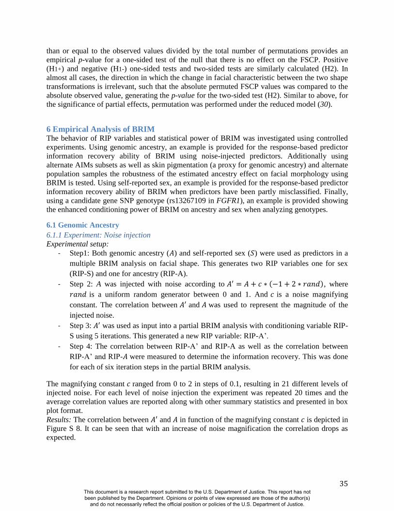
35

than or equal to the observed values divided by the total number of permutations provides an

empirical p-value for a one-sided test of the null that there is no effect on the FSCP. Positive

(H1+) and negative (H1-) one-sided tests and two-sided tests are similarly calculated (H2). In

almost all cases, the direction in which the change in facial characteristic between the two shape

transformations is irrelevant, such that the absolute permuted FSCP values was compared to the

absolute observed value, generating the p-value for the two-sided test (H2). Similar to above, for

the significance of partial effects, permutation was performed under the reduced model (30).

6 Empirical Analysis of BRIM The behavior of RIP variables and statistical power of BRIM was investigated using controlled

experiments. Using genomic ancestry, an example is provided for the response-based predictor

information recovery ability of BRIM using noise-injected predictors. Additionally using

alternate AIMs subsets as well as skin pigmentation (a proxy for genomic ancestry) and alternate

population samples the robustness of the estimated ancestry effect on facial morphology using

BRIM is tested. Using self-reported sex, an example is provided for the response-based predictor

information recovery ability of BRIM when predictors have been partly misclassified. Finally,

using a candidate gene SNP genotype (rs13267109 in FGFR1), an example is provided showing

the enhanced conditioning power of BRIM on ancestry and sex when analyzing genotypes.

6.1 Genomic Ancestry

6.1.1 Experiment: Noise injection

Experimental setup:

- Step1: Both genomic ancestry ( ) and self-reported sex ( ) were used as predictors in a

multiple BRIM analysis on facial shape. This generates two RIP variables one for sex

(RIP-S) and one for ancestry (RIP-A).

- Step 2: A was injected with noise according to ( ), where

is a uniform random generator between 0 and 1. And is a noise magnifying

constant. The correlation between and was used to represent the magnitude of the

injected noise.

- Step 3: was used as input into a partial BRIM analysis with conditioning variable RIP-

S using 5 iterations. This generated a new RIP variable: RIP-A’.

- Step 4: The correlation between RIP-A’ and RIP-A as well as the correlation between

RIP-A’ and RIP- were measured to determine the information recovery. This was done

for each of six iteration steps in the partial BRIM analysis.

The magnifying constant ranged from 0 to 2 in steps of 0.1, resulting in 21 different levels of

injected noise. For each level of noise injection the experiment was repeated 20 times and the

average correlation values are reported along with other summary statistics and presented in box

plot format.

Results: The correlation between and in function of the magnifying constant is depicted in

Figure S 8. It can be seen that with an increase of noise magnification the correlation drops as

expected.



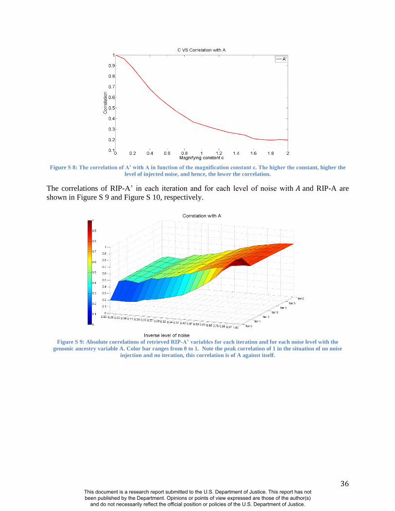
36

Figure S 8: The correlation of A’ with A in function of the magnification constant c. The higher the constant, higher the

level of injected noise, and hence, the lower the correlation.

The correlations of RIP-A’ in each iteration and for each level of noise with and RIP-A are

shown in Figure S 9 and Figure S 10, respectively.

Figure S 9: Absolute correlations of retrieved RIP-A’ variables for each iteration and for each noise level with the

genomic ancestry variable A. Color bar ranges from 0 to 1. Note the peak correlation of 1 in the situation of no noise

injection and no iteration, this correlation is of A against itself.



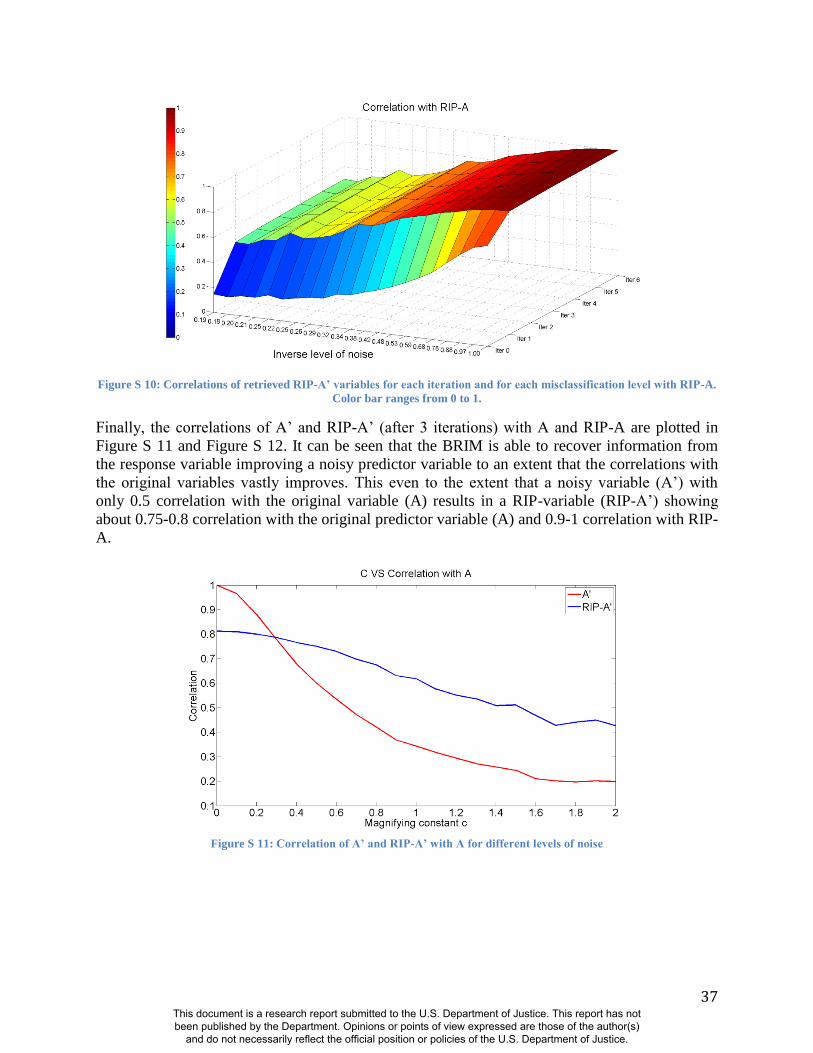
37

Figure S 10: Correlations of retrieved RIP-A’ variables for each iteration and for each misclassification level with RIP-A.

Color bar ranges from 0 to 1.

Finally, the correlations of A’ and RIP-A’ (after 3 iterations) with A and RIP-A are plotted in

Figure S 11 and Figure S 12. It can be seen that the BRIM is able to recover information from

the response variable improving a noisy predictor variable to an extent that the correlations with

the original variables vastly improves. This even to the extent that a noisy variable (A’) with

only 0.5 correlation with the original variable (A) results in a RIP-variable (RIP-A’) showing

about 0.75-0.8 correlation with the original predictor variable (A) and 0.9-1 correlation with RIP-

A.

Figure S 11: Correlation of A’ and RIP-A’ with A for different levels of noise



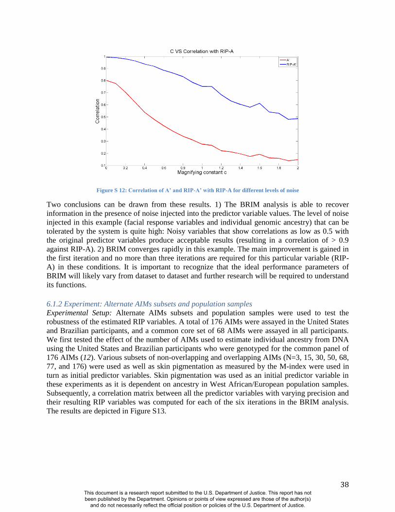
38

Figure S 12: Correlation of A’ and RIP-A’ with RIP-A for different levels of noise

Two conclusions can be drawn from these results. 1) The BRIM analysis is able to recover

information in the presence of noise injected into the predictor variable values. The level of noise

injected in this example (facial response variables and individual genomic ancestry) that can be

tolerated by the system is quite high: Noisy variables that show correlations as low as 0.5 with

the original predictor variables produce acceptable results (resulting in a correlation of > 0.9

against RIP-A). 2) BRIM converges rapidly in this example. The main improvement is gained in

the first iteration and no more than three iterations are required for this particular variable (RIP-

A) in these conditions. It is important to recognize that the ideal performance parameters of

BRIM will likely vary from dataset to dataset and further research will be required to understand

its functions.

6.1.2 Experiment: Alternate AIMs subsets and population samples

Experimental Setup: Alternate AIMs subsets and population samples were used to test the

robustness of the estimated RIP variables. A total of 176 AIMs were assayed in the United States

and Brazilian participants, and a common core set of 68 AIMs were assayed in all participants.

We first tested the effect of the number of AIMs used to estimate individual ancestry from DNA

using the United States and Brazilian participants who were genotyped for the common panel of

176 AIMs (12). Various subsets of non-overlapping and overlapping AIMs (N=3, 15, 30, 50, 68,

77, and 176) were used as well as skin pigmentation as measured by the M-index were used in

turn as initial predictor variables. Skin pigmentation was used as an initial predictor variable in

these experiments as it is dependent on ancestry in West African/European population samples.

Subsequently, a correlation matrix between all the predictor variables with varying precision and

their resulting RIP variables was computed for each of the six iterations in the BRIM analysis.

The results are depicted in Figure S13.



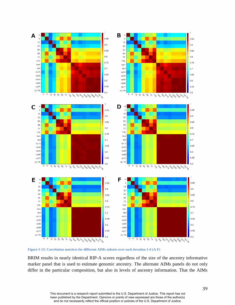
39

Figure S 13: Correlation matrices for different AIMs subsets over each iteration 1-6 (A-F)

BRIM results in nearly identical RIP-A scores regardless of the size of the ancestry informative

marker panel that is used to estimate genomic ancestry. The alternate AIMs panels do not only

differ in the particular composition, but also in levels of ancestry information. That the AIMs



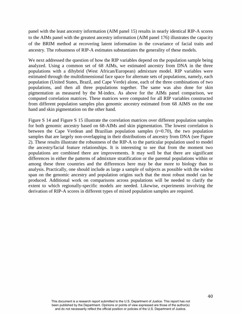
40

panel with the least ancestry information (AIM panel 15) results in nearly identical RIP-A scores

to the AIMs panel with the greatest ancestry information (AIM panel 176) illustrates the capacity

of the BRIM method at recovering latent information in the covariance of facial traits and

ancestry. The robustness of RIP-A estimates substantiates the generality of these models.

We next addressed the question of how the RIP variables depend on the population sample being

analyzed. Using a common set of 68 AIMs, we estimated ancestry from DNA in the three

populations with a dihybrid (West African/European) admixture model. RIP variables were

estimated through the multidimensional face space for alternate sets of populations, namely, each

population (United States, Brazil, and Cape Verde) alone, each of the three combinations of two

populations, and then all three populations together. The same was also done for skin

pigmentation as measured by the M-index. As above for the AIMs panel comparison, we

computed correlation matrices. These matrices were computed for all RIP variables constructed

from different population samples plus genomic ancestry estimated from 68 AIMS on the one

hand and skin pigmentation on the other hand.

Figure S 14 and Figure S 15 illustrate the correlation matrices over different population samples

for both genomic ancestry based on 68-AIMs and skin pigmentation. The lowest correlation is

between the Cape Verdean and Brazilian population samples (r=0.70), the two population

samples that are largely non-overlapping in their distributions of ancestry from DNA (see Figure

2). These results illustrate the robustness of the RIP-A to the particular population used to model

the ancestry/facial feature relationships. It is interesting to see that from the moment two

populations are combined there are improvements. It may well be that there are significant

differences in either the patterns of admixture stratification or the parental populations within or

among these three countries and the differences here may be due more to biology than to

analysis. Practically, one should include as large a sample of subjects as possible with the widest

span on the genomic ancestry and population origins such that the most robust model can be

produced. Additional work on comparisons across populations will be needed to clarify the

extent to which regionally-specific models are needed. Likewise, experiments involving the

derivation of RIP-A scores in different types of mixed population samples are required.



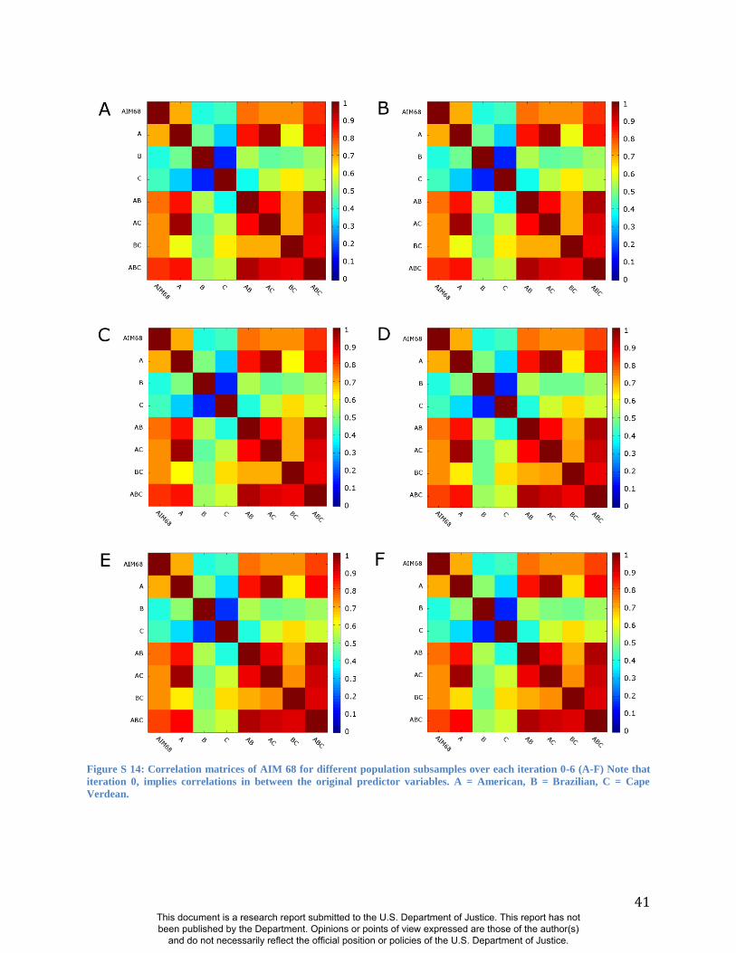
41

Figure S 14: Correlation matrices of AIM 68 for different population subsamples over each iteration 0-6 (A-F) Note that

iteration 0, implies correlations in between the original predictor variables. A = American, B = Brazilian, C = Cape

Verdean.



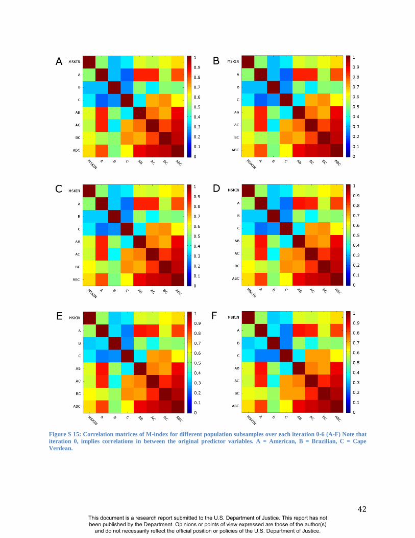
42

Figure S 15: Correlation matrices of M-index for different population subsamples over each iteration 0-6 (A-F) Note that

iteration 0, implies correlations in between the original predictor variables. A = American, B = Brazilian, C = Cape

Verdean.



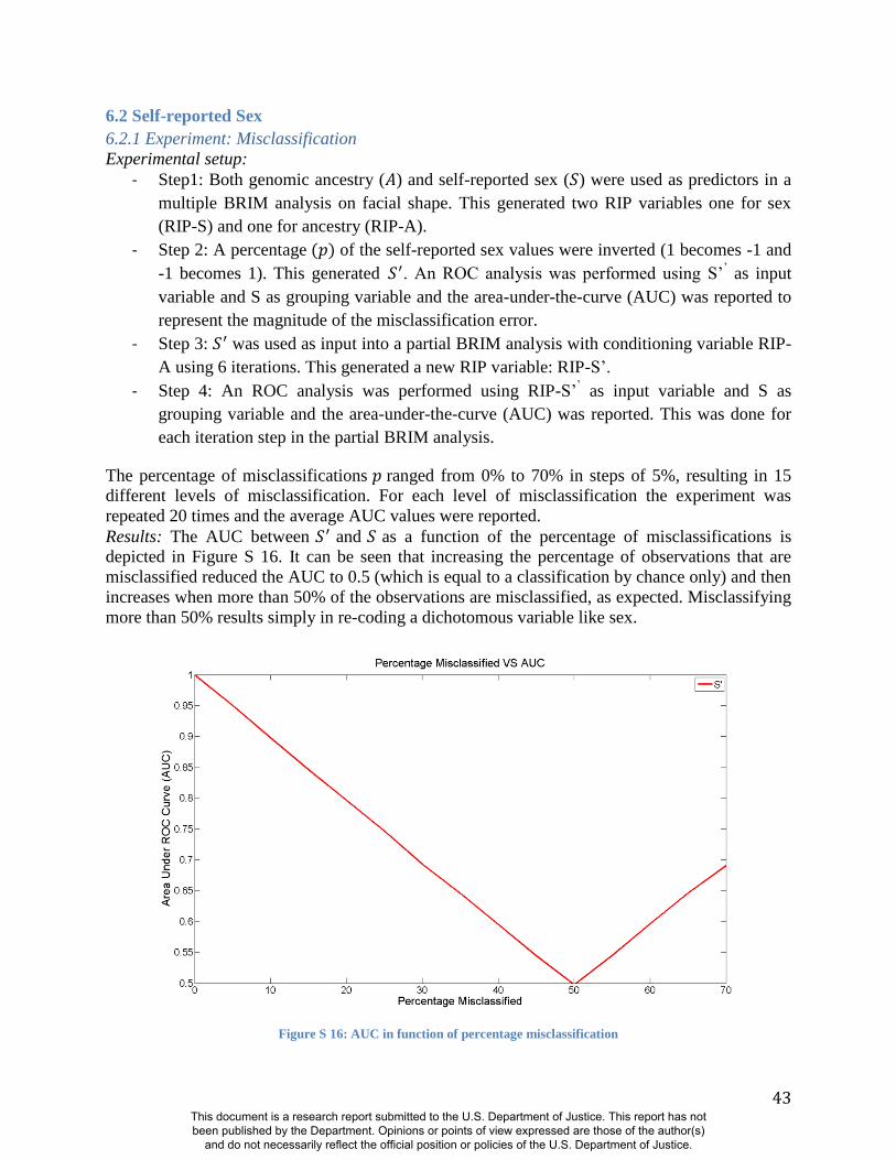
43

6.2 Self-reported Sex

6.2.1 Experiment: Misclassification

Experimental setup:

- Step1: Both genomic ancestry ( ) and self-reported sex ( ) were used as predictors in a

multiple BRIM analysis on facial shape. This generated two RIP variables one for sex

(RIP-S) and one for ancestry (RIP-A).

- Step 2: A percentage ( ) of the self-reported sex values were inverted (1 becomes -1 and

-1 becomes 1). This generated . An ROC analysis was performed using S’’ as input

variable and S as grouping variable and the area-under-the-curve (AUC) was reported to

represent the magnitude of the misclassification error.

- Step 3: was used as input into a partial BRIM analysis with conditioning variable RIP-

A using 6 iterations. This generated a new RIP variable: RIP-S’.

- Step 4: An ROC analysis was performed using RIP-S’’ as input variable and S as

grouping variable and the area-under-the-curve (AUC) was reported. This was done for

each iteration step in the partial BRIM analysis.

The percentage of misclassifications ranged from 0% to 70% in steps of 5%, resulting in 15

different levels of misclassification. For each level of misclassification the experiment was

repeated 20 times and the average AUC values were reported.

Results: The AUC between and as a function of the percentage of misclassifications is

depicted in Figure S 16. It can be seen that increasing the percentage of observations that are

misclassified reduced the AUC to 0.5 (which is equal to a classification by chance only) and then

increases when more than 50% of the observations are misclassified, as expected. Misclassifying

more than 50% results simply in re-coding a dichotomous variable like sex.

Figure S 16: AUC in function of percentage misclassification



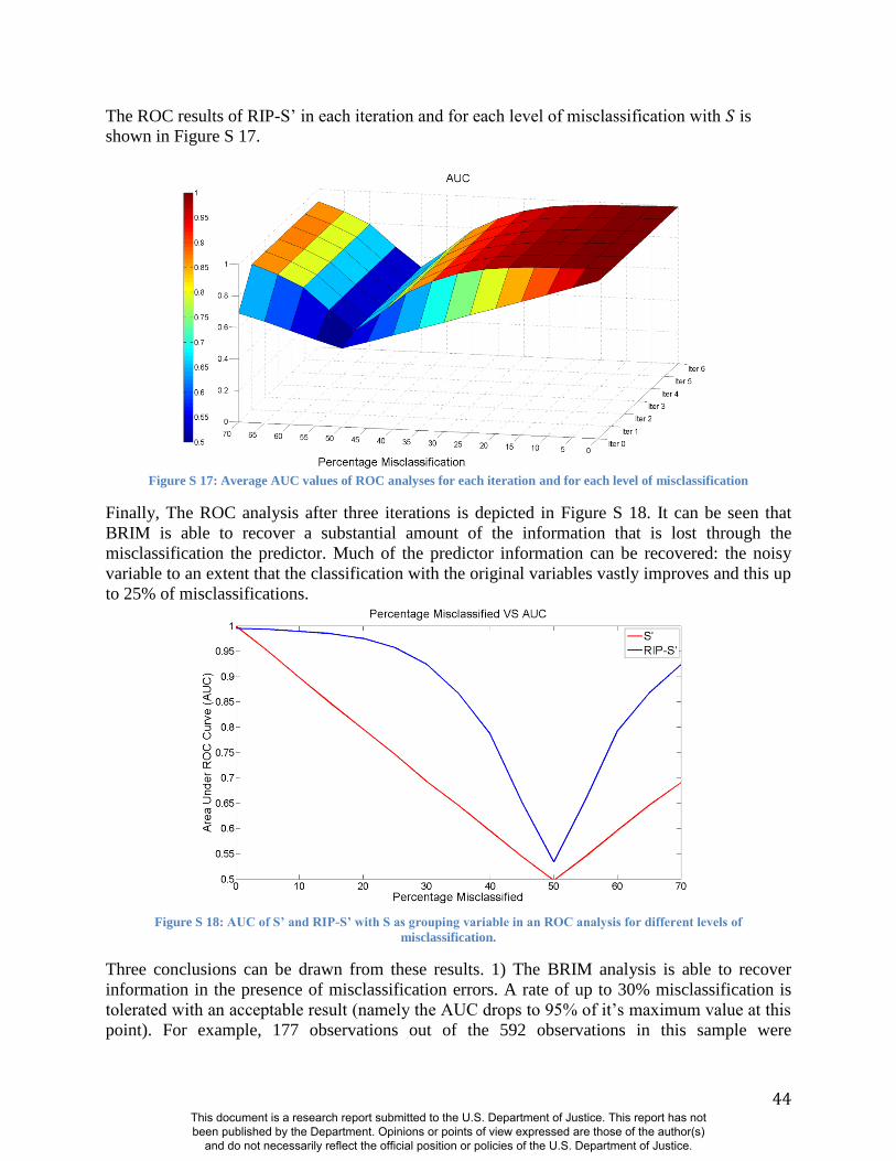
44

The ROC results of RIP-S’ in each iteration and for each level of misclassification with is

shown in Figure S 17.

Figure S 17: Average AUC values of ROC analyses for each iteration and for each level of misclassification

Finally, The ROC analysis after three iterations is depicted in Figure S 18. It can be seen that

BRIM is able to recover a substantial amount of the information that is lost through the

misclassification the predictor. Much of the predictor information can be recovered: the noisy

variable to an extent that the classification with the original variables vastly improves and this up

to 25% of misclassifications.

Figure S 18: AUC of S’ and RIP-S’ with S as grouping variable in an ROC analysis for different levels of

misclassification.

Three conclusions can be drawn from these results. 1) The BRIM analysis is able to recover

information in the presence of misclassification errors. A rate of up to 30% misclassification is

tolerated with an acceptable result (namely the AUC drops to 95% of it’s maximum value at this

point). For example, 177 observations out of the 592 observations in this sample were



45

misclassified for sex and only 18 faces were not categorized correctly by RIP-S. 2) BRIM

estimation of RIP-S in the context of facial response variables converges fast. The main

improvement is already gained in the first iteration and no more than three iterations are

required. 3) When more than 50% of the observations are misclassified, BRIM will start to

correct the ones that were not misclassified, such that a consistent re-coding of all observations

results.

6.3 Genotypes

6.3.1 Experiment: Conditioning on genomic ancestry

Experimental setup:

- Step1: Both genomic ancestry (A) and self-reported sex (S) were used as predictors in a

multiple BRIM analysis on facial morphology. This generated two RIP variables one for

sex (RIP-S) and one for ancestry (RIP).

- Step 2: For each available genetic marker a partial BRIM analysis on facial morphology

was performed conditioned only on RIP-S. For each bootstrap iteration the gene coding

(G (additive model; AA=1, AB=0 and BB=-1) and subsequent RIP-G values) were tested

for correlation with A and RIP-A.

- Step 3: For each available genetic marker a partial BRIM analysis on facial shape was

performed conditioned on RIP-S and A. For each bootstrap iteration the gene coding (G

(additive model; AA=1, AB=0 and BB=-1) and subsequent RIP-G values) were tested for

correlation with A and RIP-A.


was performed conditioned on RIP-S and RIP-A. For each bootstrap iteration the gene

coding (G (additive model; AA=1, AB=0 and BB=-1) and subsequent RIP-G values)

were tested for correlation with A and RIP-A.

Results: The correlation results of the individual 144 RIP-G variables with A and RIP-A, after

each iteration, without conditioning on ancestry are depicted using boxplots in Figure S19 and

Figure S20. It can be seen that there is a significant correlation between the original genotype G

(Iter 0) and both A and RIP-A. It is also seen that without conditioning on ancestry in effect

BRIM is transforming the initial predictor genotype variables (G) that are still, and even more

correlated with genomic ancestry.



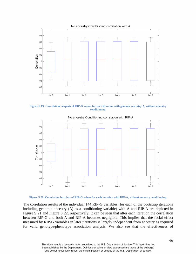
46

Figure S 19: Correlation boxplots of RIP-G values for each iteration with genomic ancestry A, without ancestry

conditioning.

Figure S 20: Correlation boxplots of RIP-G values for each iteration with RIP-A, without ancestry conditioning.

The correlation results of the individual 144 RIP-G variables (for each of the bootstrap iterations

including genomic ancestry (A) as a conditioning variable) with A and RIP-A are depicted in

Figure S 21 and Figure S 22, respectively. It can be seen that after each iteration the correlation

between RIP-G and both A and RIP-A becomes negligible. This implies that the facial effect

measured by RIP-G variables in later iterations is largely independent from ancestry as required

for valid genotype/phenotype association analysis. We also see that the effectiveness of



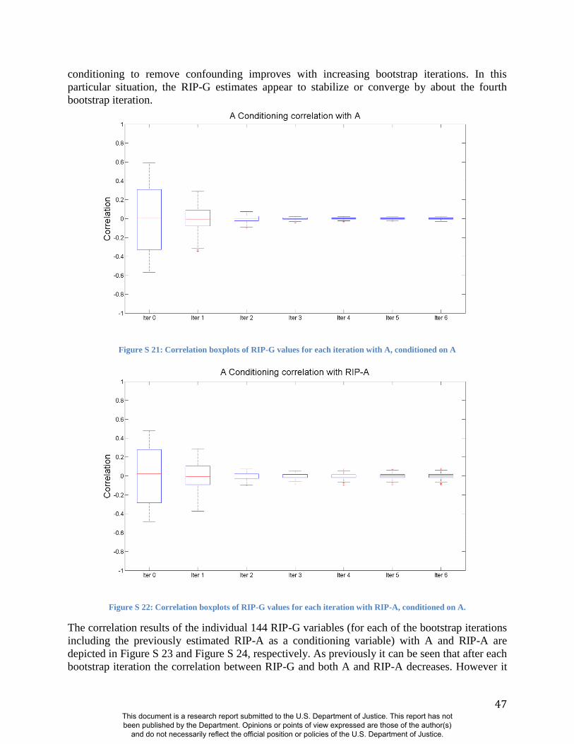
47

conditioning to remove confounding improves with increasing bootstrap iterations. In this

particular situation, the RIP-G estimates appear to stabilize or converge by about the fourth

bootstrap iteration.

Figure S 21: Correlation boxplots of RIP-G values for each iteration with A, conditioned on A

Figure S 22: Correlation boxplots of RIP-G values for each iteration with RIP-A, conditioned on A.


including the previously estimated RIP-A as a conditioning variable) with A and RIP-A are

depicted in Figure S 23 and Figure S 24, respectively. As previously it can be seen that after each

bootstrap iteration the correlation between RIP-G and both A and RIP-A decreases. However it



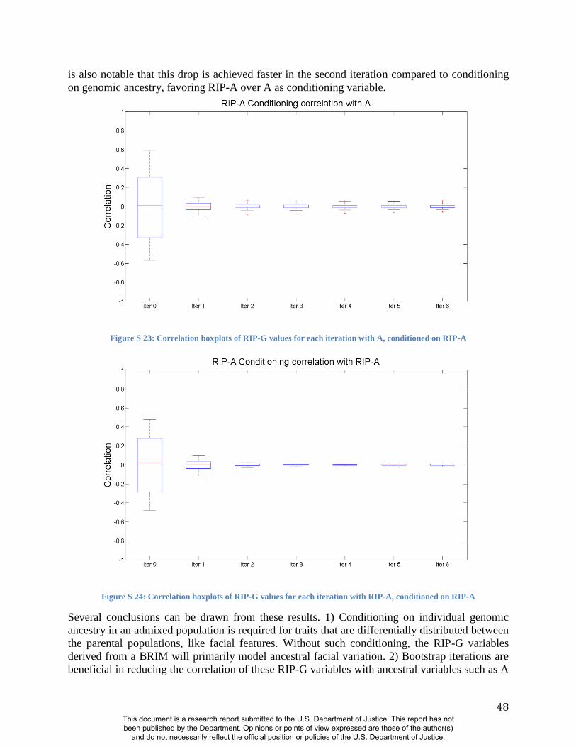
48

is also notable that this drop is achieved faster in the second iteration compared to conditioning

on genomic ancestry, favoring RIP-A over A as conditioning variable.

Figure S 23: Correlation boxplots of RIP-G values for each iteration with A, conditioned on RIP-A

Figure S 24: Correlation boxplots of RIP-G values for each iteration with RIP-A, conditioned on RIP-A

Several conclusions can be drawn from these results. 1) Conditioning on individual genomic

ancestry in an admixed population is required for traits that are differentially distributed between

the parental populations, like facial features. Without such conditioning, the RIP-G variables

derived from a BRIM will primarily model ancestral facial variation. 2) Bootstrap iterations are

beneficial in reducing the correlation of these RIP-G variables with ancestral variables such as A



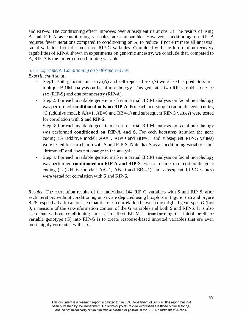
49

and RIP-A: The conditioning effect improves over subsequent iterations. 3) The results of using

A and RIP-A as conditioning variables are comparable. However, conditioning on RIP-A

requires fewer iterations compared to conditioning on A, to reduce if not eliminate all ancestral

facial variation from the measured RIP-G variables. Combined with the information recovery

capabilities of RIP-A shown in experiments on genomic ancestry, we conclude that, compared to

A, RIP-A is the preferred conditioning variable.

6.3.2 Experiment: Conditioning on Self-reported Sex

Experimental setup:

- Step1: Both genomic ancestry (A) and self-reported sex (S) were used as predictors in a

multiple BRIM analysis on facial morphology. This generates two RIP variables one for

sex (RIP-S) and one for ancestry (RIP-A).


was performed conditioned only on RIP-A. For each bootstrap iteration the gene coding

(G (additive model; AA=1, AB=0 and BB=-1) and subsequent RIP-G values) were tested

for correlation with S and RIP-S.


was performed conditioned on RIP-A and S. For each bootstrap iteration the gene


were tested for correlation with S and RIP-S. Note that S as a conditioning variable is not

“brimmed” and does not change in the analysis.


was performed conditioned on RIP-A and RIP-S. For each bootstrap iteration the gene


were tested for correlation with S and RIP-S.

Results: The correlation results of the individual 144 RIP-G variables with S and RIP-S, after

each iteration, without conditioning on sex are depicted using boxplots in Figure S 25 and Figure

S 26 respectively. It can be seen that there is a correlation between the original genotypes G (Iter

0, a measure of the sex-information content of the G variable) and both S and RIP-S. It is also

seen that without conditioning on sex in effect BRIM is transforming the initial predictor

variable genotype (G) into RIP-G is to create response-based imputed variables that are even

more highly correlated with sex.



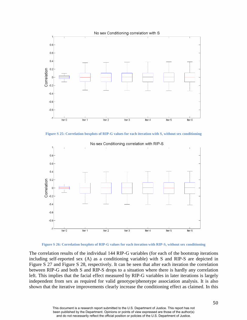
50

Figure S 25: Correlation boxplots of RIP-G values for each iteration with S, without sex conditioning

Figure S 26: Correlation boxplots of RIP-G values for each iteration with RIP-S, without sex conditioning


including self-reported sex (A) as a conditioning variable) with S and RIP-S are depicted in

Figure S 27 and Figure S 28, respectively. It can be seen that after each iteration the correlation

between RIP-G and both S and RIP-S drops to a situation where there is hardly any correlation

left. This implies that the facial effect measured by RIP-G variables in later iterations is largely

independent from sex as required for valid genotype/phenotype association analysis. It is also

shown that the iterative improvements clearly increase the conditioning effect as claimed. In this



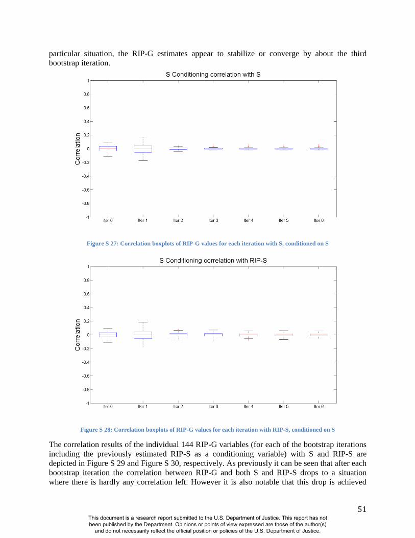
51

particular situation, the RIP-G estimates appear to stabilize or converge by about the third

bootstrap iteration.

Figure S 27: Correlation boxplots of RIP-G values for each iteration with S, conditioned on S

Figure S 28: Correlation boxplots of RIP-G values for each iteration with RIP-S, conditioned on S


including the previously estimated RIP-S as a conditioning variable) with S and RIP-S are

depicted in Figure S 29 and Figure S 30, respectively. As previously it can be seen that after each

bootstrap iteration the correlation between RIP-G and both S and RIP-S drops to a situation

where there is hardly any correlation left. However it is also notable that this drop is achieved



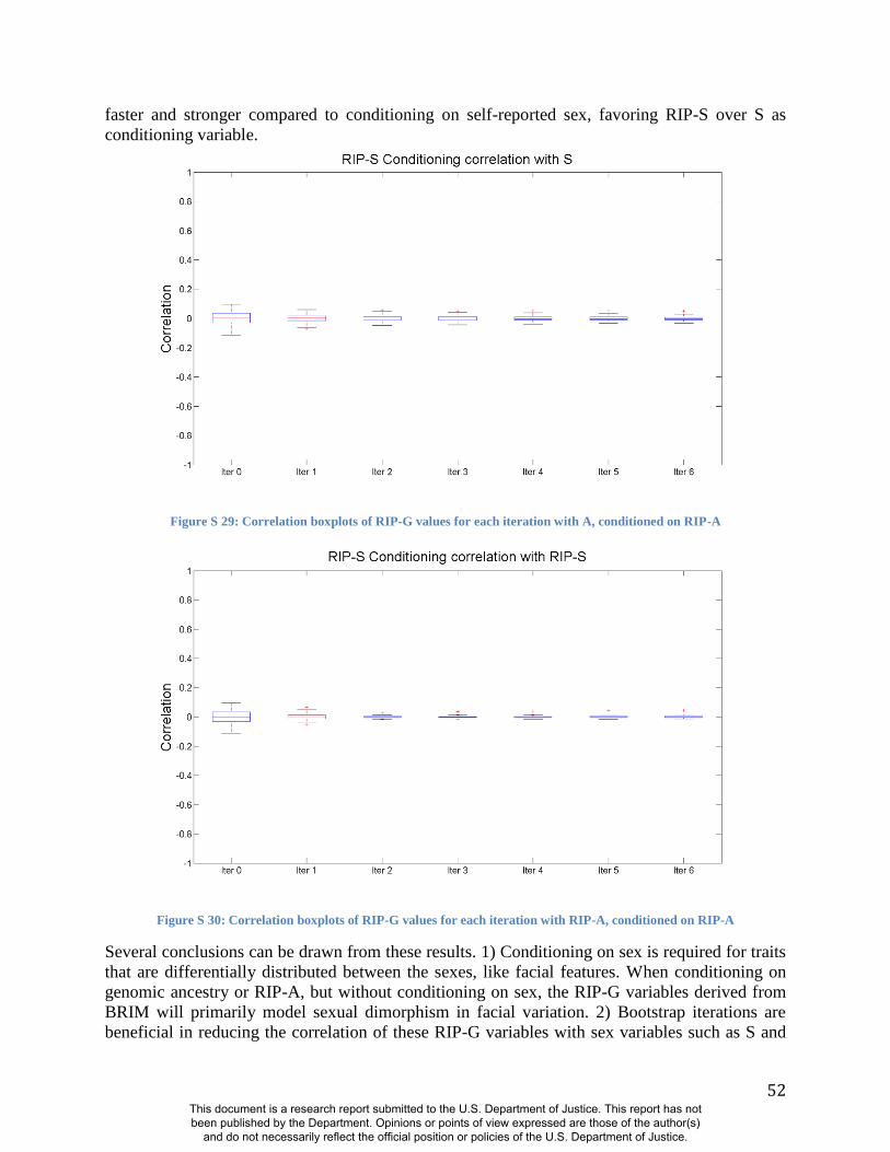
52

faster and stronger compared to conditioning on self-reported sex, favoring RIP-S over S as

conditioning variable.

Figure S 29: Correlation boxplots of RIP-G values for each iteration with A, conditioned on RIP-A

Figure S 30: Correlation boxplots of RIP-G values for each iteration with RIP-A, conditioned on RIP-A

Several conclusions can be drawn from these results. 1) Conditioning on sex is required for traits

that are differentially distributed between the sexes, like facial features. When conditioning on

genomic ancestry or RIP-A, but without conditioning on sex, the RIP-G variables derived from

BRIM will primarily model sexual dimorphism in facial variation. 2) Bootstrap iterations are

beneficial in reducing the correlation of these RIP-G variables with sex variables such as S and



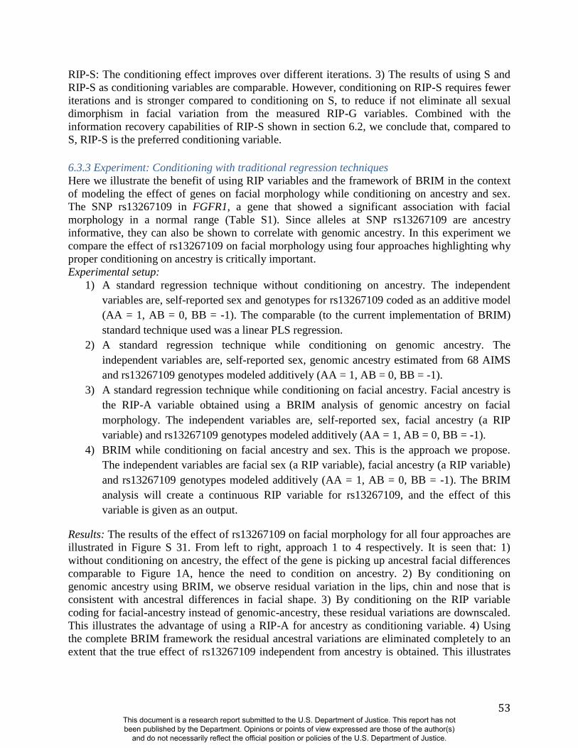
53

RIP-S: The conditioning effect improves over different iterations. 3) The results of using S and

RIP-S as conditioning variables are comparable. However, conditioning on RIP-S requires fewer

iterations and is stronger compared to conditioning on S, to reduce if not eliminate all sexual

dimorphism in facial variation from the measured RIP-G variables. Combined with the

information recovery capabilities of RIP-S shown in section 6.2, we conclude that, compared to

S, RIP-S is the preferred conditioning variable.

6.3.3 Experiment: Conditioning with traditional regression techniques

Here we illustrate the benefit of using RIP variables and the framework of BRIM in the context

of modeling the effect of genes on facial morphology while conditioning on ancestry and sex.

The SNP rs13267109 in FGFR1, a gene that showed a significant association with facial

morphology in a normal range (Table S1). Since alleles at SNP rs13267109 are ancestry

informative, they can also be shown to correlate with genomic ancestry. In this experiment we

compare the effect of rs13267109 on facial morphology using four approaches highlighting why

proper conditioning on ancestry is critically important.

Experimental setup:

1) A standard regression technique without conditioning on ancestry. The independent

variables are, self-reported sex and genotypes for rs13267109 coded as an additive model

(AA = 1, AB = 0, BB = -1). The comparable (to the current implementation of BRIM)

standard technique used was a linear PLS regression.

2) A standard regression technique while conditioning on genomic ancestry. The

independent variables are, self-reported sex, genomic ancestry estimated from 68 AIMS

and rs13267109 genotypes modeled additively (AA = 1, AB = 0, BB = -1).

3) A standard regression technique while conditioning on facial ancestry. Facial ancestry is

the RIP-A variable obtained using a BRIM analysis of genomic ancestry on facial

morphology. The independent variables are, self-reported sex, facial ancestry (a RIP

variable) and rs13267109 genotypes modeled additively (AA = 1, AB = 0, BB = -1).

4) BRIM while conditioning on facial ancestry and sex. This is the approach we propose.

The independent variables are facial sex (a RIP variable), facial ancestry (a RIP variable)

and rs13267109 genotypes modeled additively (AA = 1, AB = 0, BB = -1). The BRIM

analysis will create a continuous RIP variable for rs13267109, and the effect of this

variable is given as an output.

Results: The results of the effect of rs13267109 on facial morphology for all four approaches are

illustrated in Figure S 31. From left to right, approach 1 to 4 respectively. It is seen that: 1)

without conditioning on ancestry, the effect of the gene is picking up ancestral facial differences

comparable to Figure 1A, hence the need to condition on ancestry. 2) By conditioning on

genomic ancestry using BRIM, we observe residual variation in the lips, chin and nose that is

consistent with ancestral differences in facial shape. 3) By conditioning on the RIP variable

coding for facial-ancestry instead of genomic-ancestry, these residual variations are downscaled.

This illustrates the advantage of using a RIP-A for ancestry as conditioning variable. 4) Using

the complete BRIM framework the residual ancestral variations are eliminated completely to an

extent that the true effect of rs13267109 independent from ancestry is obtained. This illustrates



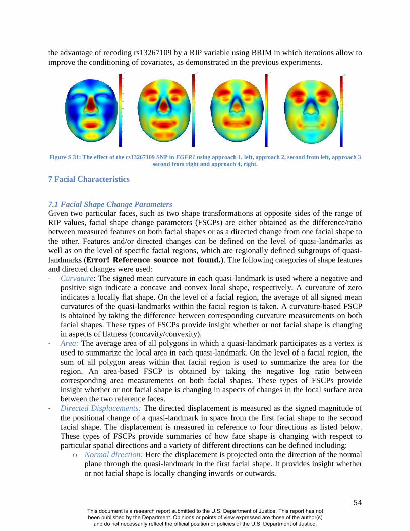
54

the advantage of recoding rs13267109 by a RIP variable using BRIM in which iterations allow to

improve the conditioning of covariates, as demonstrated in the previous experiments.

Figure S 31: The effect of the rs13267109 SNP in FGFR1 using approach 1, left, approach 2, second from left, approach 3

second from right and approach 4, right.

7 Facial Characteristics

7.1 Facial Shape Change Parameters

Given two particular faces, such as two shape transformations at opposite sides of the range of

RIP values, facial shape change parameters (FSCPs) are either obtained as the difference/ratio

between measured features on both facial shapes or as a directed change from one facial shape to

the other. Features and/or directed changes can be defined on the level of quasi-landmarks as

well as on the level of specific facial regions, which are regionally defined subgroups of quasi-

landmarks (Error! Reference source not found.). The following categories of shape features

and directed changes were used:

- Curvature: The signed mean curvature in each quasi-landmark is used where a negative and

positive sign indicate a concave and convex local shape, respectively. A curvature of zero

indicates a locally flat shape. On the level of a facial region, the average of all signed mean

curvatures of the quasi-landmarks within the facial region is taken. A curvature-based FSCP

is obtained by taking the difference between corresponding curvature measurements on both

facial shapes. These types of FSCPs provide insight whether or not facial shape is changing

in aspects of flatness (concavity/convexity).

- Area: The average area of all polygons in which a quasi-landmark participates as a vertex is

used to summarize the local area in each quasi-landmark. On the level of a facial region, the

sum of all polygon areas within that facial region is used to summarize the area for the

region. An area-based FSCP is obtained by taking the negative log ratio between

corresponding area measurements on both facial shapes. These types of FSCPs provide

insight whether or not facial shape is changing in aspects of changes in the local surface area

between the two reference faces.

- Directed Displacements: The directed displacement is measured as the signed magnitude of

the positional change of a quasi-landmark in space from the first facial shape to the second

facial shape. The displacement is measured in reference to four directions as listed below.

These types of FSCPs provide summaries of how face shape is changing with respect to

particular spatial directions and a variety of different directions can be defined including:

o Normal direction: Here the displacement is projected onto the direction of the normal

plane through the quasi-landmark in the first facial shape. It provides insight whether

or not facial shape is locally changing inwards or outwards.



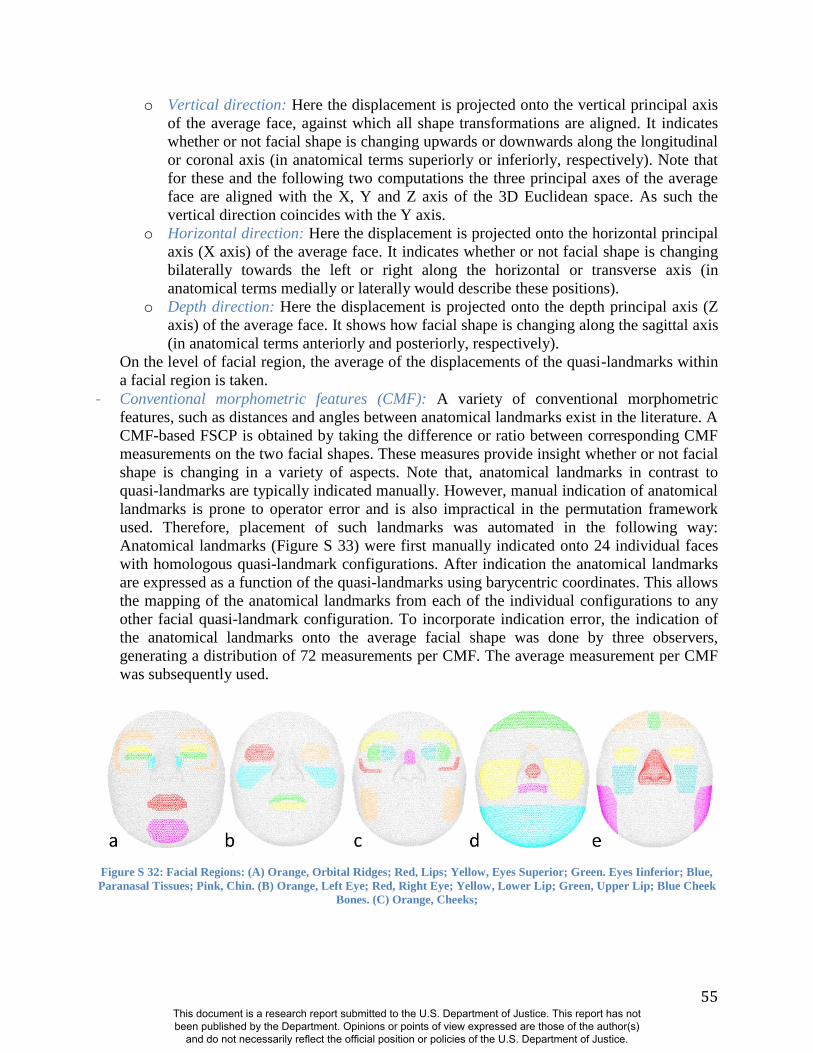
55

o Vertical direction: Here the displacement is projected onto the vertical principal axis

of the average face, against which all shape transformations are aligned. It indicates

whether or not facial shape is changing upwards or downwards along the longitudinal

or coronal axis (in anatomical terms superiorly or inferiorly, respectively). Note that

for these and the following two computations the three principal axes of the average

face are aligned with the X, Y and Z axis of the 3D Euclidean space. As such the

vertical direction coincides with the Y axis.

o Horizontal direction: Here the displacement is projected onto the horizontal principal

axis (X axis) of the average face. It indicates whether or not facial shape is changing

bilaterally towards the left or right along the horizontal or transverse axis (in

anatomical terms medially or laterally would describe these positions).

o Depth direction: Here the displacement is projected onto the depth principal axis (Z

axis) of the average face. It shows how facial shape is changing along the sagittal axis

(in anatomical terms anteriorly and posteriorly, respectively).

On the level of facial region, the average of the displacements of the quasi-landmarks within

a facial region is taken.

- Conventional morphometric features (CMF): A variety of conventional morphometric

features, such as distances and angles between anatomical landmarks exist in the literature. A

CMF-based FSCP is obtained by taking the difference or ratio between corresponding CMF

measurements on the two facial shapes. These measures provide insight whether or not facial

shape is changing in a variety of aspects. Note that, anatomical landmarks in contrast to

quasi-landmarks are typically indicated manually. However, manual indication of anatomical

landmarks is prone to operator error and is also impractical in the permutation framework

used. Therefore, placement of such landmarks was automated in the following way:

Anatomical landmarks (Figure S 33) were first manually indicated onto 24 individual faces

with homologous quasi-landmark configurations. After indication the anatomical landmarks

are expressed as a function of the quasi-landmarks using barycentric coordinates. This allows

the mapping of the anatomical landmarks from each of the individual configurations to any

other facial quasi-landmark configuration. To incorporate indication error, the indication of

the anatomical landmarks onto the average facial shape was done by three observers,

generating a distribution of 72 measurements per CMF. The average measurement per CMF

was subsequently used.

Figure S 32: Facial Regions: (A) Orange, Orbital Ridges; Red, Lips; Yellow, Eyes Superior; Green. Eyes Iinferior; Blue,

Paranasal Tissues; Pink, Chin. (B) Orange, Left Eye; Red, Right Eye; Yellow, Lower Lip; Green, Upper Lip; Blue Cheek

Bones. (C) Orange, Cheeks;



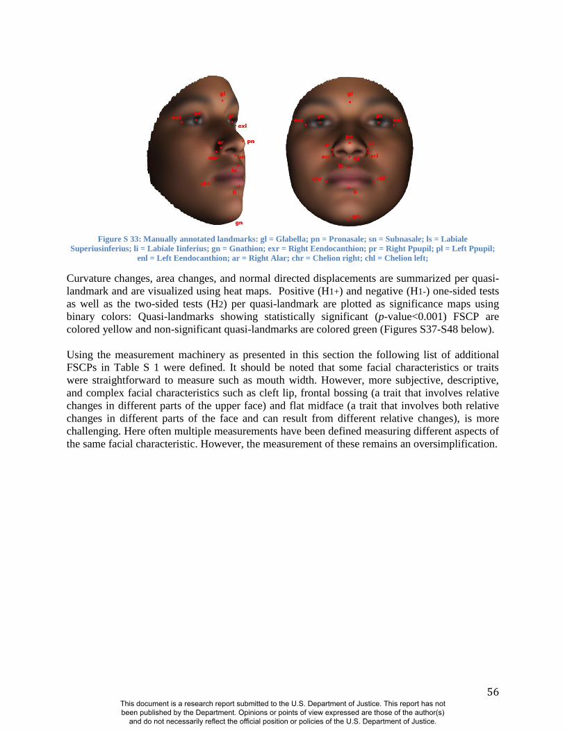
56

Figure S 33: Manually annotated landmarks: gl = Glabella; pn = Pronasale; sn = Subnasale; ls = Labiale

Superiusinferius; li = Labiale Iinferius; gn = Gnathion; exr = Right Eendocanthion; pr = Right Ppupil; pl = Left Ppupil;

enl = Left Eendocanthion; ar = Right Alar; chr = Chelion right; chl = Chelion left;

Curvature changes, area changes, and normal directed displacements are summarized per quasi-

landmark and are visualized using heat maps. Positive (H1+) and negative (H1-) one-sided tests

as well as the two-sided tests (H2) per quasi-landmark are plotted as significance maps using

binary colors: Quasi-landmarks showing statistically significant (p-value<0.001) FSCP are

colored yellow and non-significant quasi-landmarks are colored green (Figures S37-S48 below).

Using the measurement machinery as presented in this section the following list of additional

FSCPs in Table S 1 were defined. It should be noted that some facial characteristics or traits

were straightforward to measure such as mouth width. However, more subjective, descriptive,

and complex facial characteristics such as cleft lip, frontal bossing (a trait that involves relative

changes in different parts of the upper face) and flat midface (a trait that involves both relative

changes in different parts of the face and can result from different relative changes), is more

challenging. Here often multiple measurements have been defined measuring different aspects of

the same facial characteristic. However, the measurement of these remains an oversimplification.



57

Table S 1: List of local FSCPs measured. C = curvature, S = area, LM = landmark, N = normal displacement, P = point, B

= shape transformation -X times the standard deviation of RIP values, A = shape transformation +X times the standard

deviation of RIP values, σx,y,z the standard deviation of quasi-landmarks in the x,y or z direction (used as surrogate for

length and width measurements), θ = angle measurement, = distance between two points, = distance in the X, Y, or

Z direction, = vector from point to point .

Facial

Characteristic

I

D

Explanation Technical Formulation

Malar flattening A Change in surface curvature at the

cheekbones

B Change in variation or dispersion in

position (standard deviation) along the

antero-posterior (sagittal) axis of the

cheekbones

|

|

C Inward/outward movement of the medial

part of the midface, in relation to the

lateral part of the lower face

| |

Square/round

face

A Change in similarity between facial

contours and a square (Figure S 34)

Take a border projection of each shape

transformation and compare it with a fitted square:

|√ ∑ (

( ( )))

√ ∑ (

( ( )))

|

The square fitted to each of the morphs is defined

by placing the 2 vertical lines at the most lateral

positions of the facial border (left and right) and

the 2 horizontal lines at the most superior and

inferior positions of the facial border.

Micrognathia A Inward/outward movement of the chin B Area increase/decrease of the size of the

chin | (

)|

C Change in distance between labiale

inferius and gnathion, along the vertical

(longitudinal) axis

| (

)

(

)|

Microcephaly A Change in size of the circle fitted to the

surface of the forehead. The circle is

placed in the transverse plane, halfway the

glabella and the top of the face (Figure S 35)

Take the intersection plane with the facial mesh

(through point halfway between glabella and top of

head, parallel to the XZ plane), fit a circle through

the intersection points, and take radius as

approximate for head circumference

B Inward/outward movement of the upper

face | |

Midface

retrusion / Flat

midface

A Inward/outward movement of the midface

in relation to the inward/outward

movement of the upper and lower face

| |

B Change in surface curvature at the midface |

| Frontal bossing A Inward or outward movement of the

bilateral parts of the upper face, relative to

the movement of the metopic ridge

| |

Metopic ridge A Change in curvature at the surface over |

|



58

prominent the metopic ridge

Face long A Change in height-width ratio of the entire

face | (

) (

)|

Forehead short A Change in height of the upper face |

|

Supraorbital

ridge

underdeveloped

A Inward/outward movement of the

supraorbital ridge | |

B Displacement of the supraorbital ridge

along the antero-posterior (sagittal) axis. | ( ( )

( ))|

Forehead

sloping

A Inward/outward movement of the upper

face | |

B Change in angle that the antero-posterior

(sagittal) axis makes with the anterior

surface of the forehead, at the intersection

with the sagittal (medial) plane, through

the glabella

| ( )

(

)| where TopForehead is the most superior point of

the intersection line between the ZY-plane through

the glabella and the facial mesh.

Forehead

narrow/ broad

A Change in width of the upper face |

|

Shallow orbits A

AN

D

Inward/outward movement of the

orbital ridges | |

B Inward/outward movement of the

supraorbital ridge | |

C Inward/outward movement of the

infraorbital ridge | |

D

AN

D

Change in surface curvature at the

orbital ridges |

|

E Change in surface curvature at the

supraorbital ridge |

|

F Change in surface curvature at the

infraorbital ridge |

|

Superiorly

oriented orbits

A Change in surface curvature at the

superior half of the eye, compared to the

change in surface curvature at the inferior

half of the eye.

|(

)

(

)|

B Inward/outward movement of the superior

half of the eye, compared to the

inward/outward movement of the inferior

half of the eye.

| |

C Area increase/decrease of the superior half

of the eye, compared to the area

increase/decrease of the inferior half of the

eye.

| (

) (

)|

Palpebral

fissures

downslanted

A Change in distance along the vertical

(longitudinal) axis from the average

position of the medial half of the eye, to

the average position of the lateral half of

the eye.

| ( ( ) ( )

)

( ( ) ( )

)|

B Change in angle between the principal

axis of the left eye and the principal axis

of the right eye

| (

)

(

)|



59

Eyes widely

spaced

A Change in interpupillary distance | (

)

(

)| B Change in outer canthal distance

| (

)

(

)|

C Change in distance along the medio-lateral

(horizontal) axis from the average position

of the left eye, to the average position of

the right eye.

| ( ( ) ( )

)

( ( ) ( )

)|

Proptosis A

AN

D

Movement of the eyes along the

antero-posterior (sagittal) axis | ( ( ) ( ))|

B

AN

D

Movement of the lateral half of

the eyes along the antero-

posterior (sagittal) axis. | (

( )

( ))|

C Movement of the medial half of

the eyes along the antero-


( )

( ))|

D

AN

D

Movement of the superior half

of the eyes along the antero-


( )

( ))|

E Movement of the inferior half

of the eyes along the antero-


( )

( ))|

F

NO

T

Change in distance along the

antero-posterior (sagittal) axis

from the average position of the

superior half of the eyes, to the

average position of the inferior

half of the eyes. (This indicates

‘superiorly oriented orbits’)

| ( ( ) ( )

)

( ( ) ( )

)|

Nasal ridge

narrow

A Change in width of the nasal ridge |

|

B

AN

D

Change in curvature at the surface

over the nasal ridge, compared to the

change in surface curvature at the

paranasal tissues

|(

)

(

)|

C Change in surface curvature at the

nasal ridge |

|

D Change in surface curvature at the

paranasal tissues

Nasal ridge

retruded

A Inward/outward movement of the nasal

ridge | |

Nasal bridge

depressed

A Inward/outward movement of the nasal

bridge | |

Nasal bridge

wide

A Change in surface curvature at the nasal

bridge |

|

B Change in width of the nasal bridge |

|



60

Nose wide A Change in distance between alar curvature

left and right | (

)

(

)|

B Change in distance between alare left and

right | (

)

(

)| Nose snubbed A Change in angle between columella

(represented as a vector from subnasale to

pronasale) and philtrum (represented as a

vector from subnasale to labiale superius)

| (

)

(

)|

Nares

anteverted

A Change in distance along the vertical

(longitudinal) axis between subnasale and

pronasale

| (

)

(

)|

Cleft lip A Area increase/decrease of the philtrum

| (

)|

B Inward/outward movement of the philtrum C Change in surface curvature of the

philtrum

D Area increase/decrease of the nose

| (

)|

E Inward/outward movement of the nose F Change in surface curvature of the nose

Mouth wide A Change in distance between left and right

chelion | (

)

(

)| Vermilion upper

lip thick

A Area increase/decrease of the upper lip

(upper vermilion) | (

)|

Vermilion lower

lip thick

A Area increase/decrease of the lower lip

(lower vermilion) | (

)|

Lips thick A Area increase/decrease of the lips

| (

)|

Maxilla

prominent

A Movement of the midface along the

antero-posterior (sagittal) axis | ( ( )) ( ( ))|

B Inward/outward movement of the medial

part of the midface, in relation to the

lateral part of the lower face

| |

Philtrum long A Change in length of the philtrum

(represented as a vector from subnasale to

labiale superius)

| (

)

(

)|

Sunken cheeks A Area increase/decrease of the cheeks

| (

)|

Large eyes A Area increase/decrease of the eyes

| (

)|



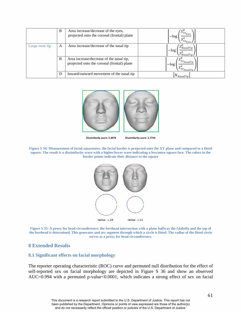
61

B Area increase/decrease of the eyes,

projected onto the coronal (frontal) plane | (

)|

Large nose tip A Area increase/decrease of the nasal tip | (

)|

B Area increase/decrease of the nasal tip,

projected onto the coronal (frontal) plane | (

)|

D Inward/outward movement of the nasal tip | |

Figure S 34: Measurement of facial squareness: the facial border is projected onto the XY plane and compared to a fitted

square. The result is a dissimilarity score with a higher/lower score indicating a less/more square face. The colors in the

border points indicate their distance to the square

Figure S 35: A proxy for head circumference: the forehead intersection with a plane halfway the Glabella and the top of

the forehead is determined. This generates and arc segment through which a circle is fitted. The radius of the fitted circle

serves as a proxy for head circumference.

8 Extended Results

8.1 Significant effects on facial morphology

The reporter operating characteristic (ROC) curve and permuted null distribution for the effect of

self-reported sex on facial morphology are depicted in Figure S 36 and show an observed

AUC=0.994 with a permuted p-value<0.0001, which indicates a strong effect of sex on facial



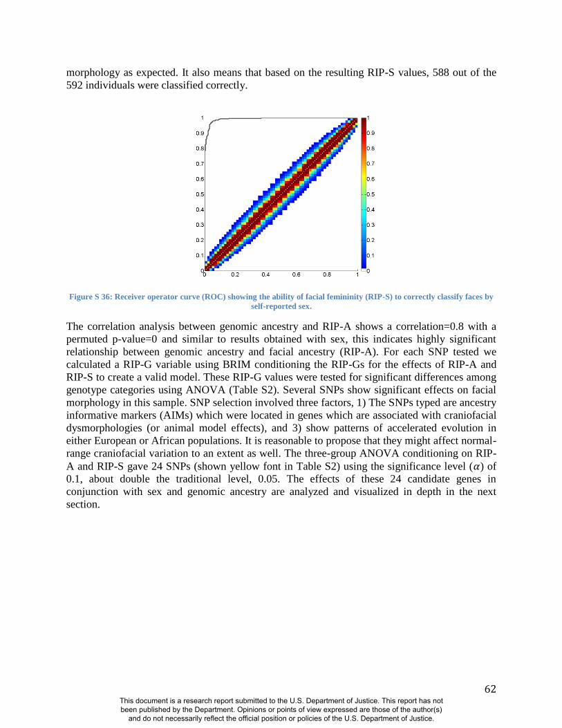
62

morphology as expected. It also means that based on the resulting RIP-S values, 588 out of the

592 individuals were classified correctly.

Figure S 36: Receiver operator curve (ROC) showing the ability of facial femininity (RIP-S) to correctly classify faces by

self-reported sex.

The correlation analysis between genomic ancestry and RIP-A shows a correlation=0.8 with a

permuted p-value=0 and similar to results obtained with sex, this indicates highly significant

relationship between genomic ancestry and facial ancestry (RIP-A). For each SNP tested we

calculated a RIP-G variable using BRIM conditioning the RIP-Gs for the effects of RIP-A and

RIP-S to create a valid model. These RIP-G values were tested for significant differences among

genotype categories using ANOVA (Table S2). Several SNPs show significant effects on facial

morphology in this sample. SNP selection involved three factors, 1) The SNPs typed are ancestry

informative markers (AIMs) which were located in genes which are associated with craniofacial

dysmorphologies (or animal model effects), and 3) show patterns of accelerated evolution in

either European or African populations. It is reasonable to propose that they might affect normal-

range craniofacial variation to an extent as well. The three-group ANOVA conditioning on RIP-

A and RIP-S gave 24 SNPs (shown yellow font in Table S2) using the significance level ( ) of

0.1, about double the traditional level, 0.05. The effects of these 24 candidate genes in

conjunction with sex and genomic ancestry are analyzed and visualized in depth in the next

section.



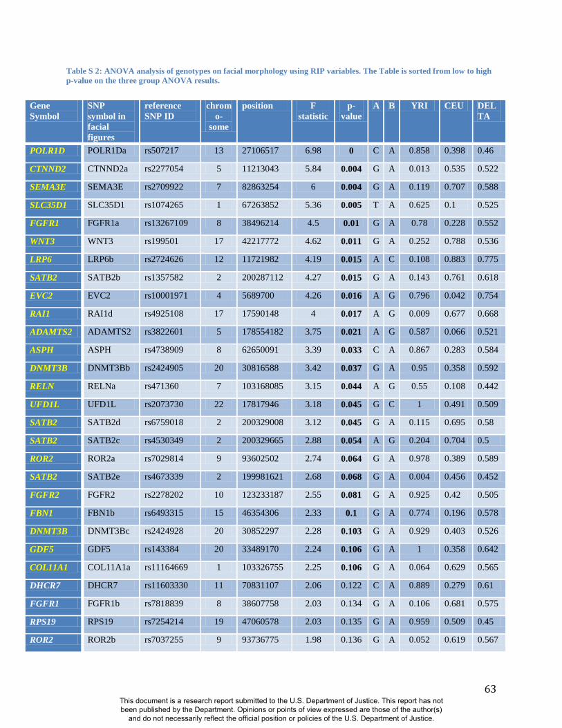
63

Table S 2: ANOVA analysis of genotypes on facial morphology using RIP variables. The Table is sorted from low to high

p-value on the three group ANOVA results.

Gene

Symbol

SNP

symbol in

facial

figures

reference

SNP ID

chrom

o-

some

position F

statistic

p-

value

A B YRI CEU DEL

TA

POLR1D POLR1Da rs507217 13 27106517 6.98 0 C A 0.858 0.398 0.46

CTNND2 CTNND2a rs2277054 5 11213043 5.84 0.004 G A 0.013 0.535 0.522

SEMA3E SEMA3E rs2709922 7 82863254 6 0.004 G A 0.119 0.707 0.588

SLC35D1 SLC35D1 rs1074265 1 67263852 5.36 0.005 T A 0.625 0.1 0.525

FGFR1 FGFR1a rs13267109 8 38496214 4.5 0.01 G A 0.78 0.228 0.552

WNT3 WNT3 rs199501 17 42217772 4.62 0.011 G A 0.252 0.788 0.536

LRP6 LRP6b rs2724626 12 11721982 4.19 0.015 A C 0.108 0.883 0.775

SATB2 SATB2b rs1357582 2 200287112 4.27 0.015 G A 0.143 0.761 0.618

EVC2 EVC2 rs10001971 4 5689700 4.26 0.016 A G 0.796 0.042 0.754

RAI1 RAI1d rs4925108 17 17590148 4 0.017 A G 0.009 0.677 0.668

ADAMTS2 ADAMTS2 rs3822601 5 178554182 3.75 0.021 A G 0.587 0.066 0.521

ASPH ASPH rs4738909 8 62650091 3.39 0.033 C A 0.867 0.283 0.584

DNMT3B DNMT3Bb rs2424905 20 30816588 3.42 0.037 G A 0.95 0.358 0.592

RELN RELNa rs471360 7 103168085 3.15 0.044 A G 0.55 0.108 0.442

UFD1L UFD1L rs2073730 22 17817946 3.18 0.045 G C 1 0.491 0.509

SATB2 SATB2d rs6759018 2 200329008 3.12 0.045 G A 0.115 0.695 0.58

SATB2 SATB2c rs4530349 2 200329665 2.88 0.054 A G 0.204 0.704 0.5

ROR2 ROR2a rs7029814 9 93602502 2.74 0.064 G A 0.978 0.389 0.589

SATB2 SATB2e rs4673339 2 199981621 2.68 0.068 G A 0.004 0.456 0.452

FGFR2 FGFR2 rs2278202 10 123233187 2.55 0.081 G A 0.925 0.42 0.505

FBN1 FBN1b rs6493315 15 46354306 2.33 0.1 G A 0.774 0.196 0.578

DNMT3B DNMT3Bc rs2424928 20 30852297 2.28 0.103 G A 0.929 0.403 0.526

GDF5 GDF5 rs143384 20 33489170 2.24 0.106 G A 1 0.358 0.642

COL11A1 COL11A1a rs11164669 1 103326755 2.25 0.106 G A 0.064 0.629 0.565

DHCR7 DHCR7 rs11603330 11 70831107 2.06 0.122 C A 0.889 0.279 0.61

FGFR1 FGFR1b rs7818839 8 38607758 2.03 0.134 G A 0.106 0.681 0.575

RPS19 RPS19 rs7254214 19 47060578 2.03 0.135 G A 0.959 0.509 0.45

ROR2 ROR2b rs7037255 9 93736775 1.98 0.136 G A 0.052 0.619 0.567



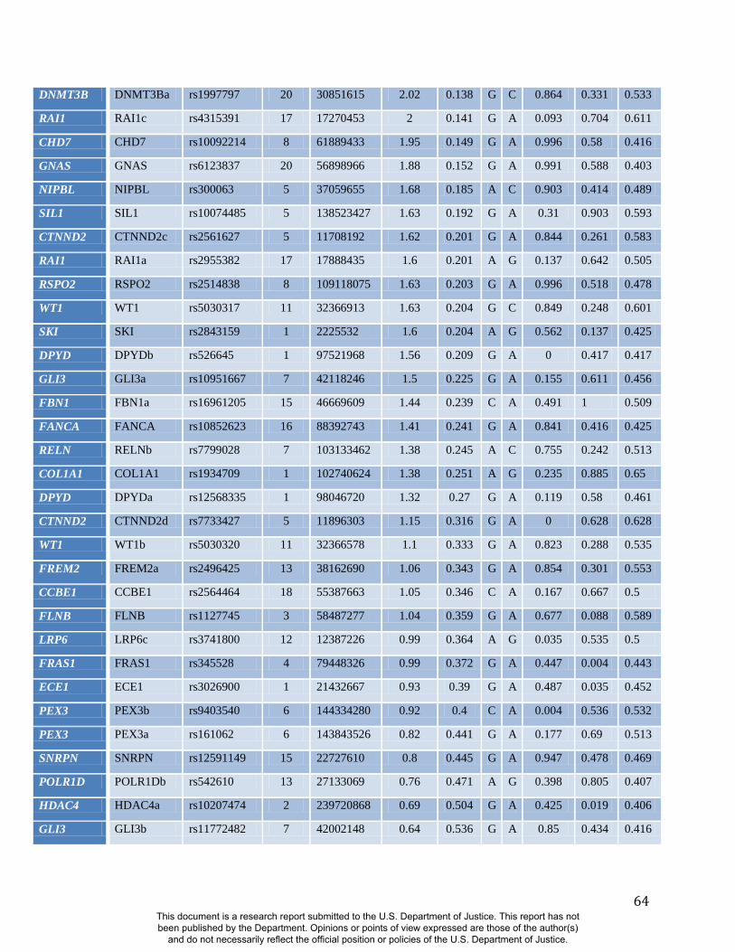
64

DNMT3B DNMT3Ba rs1997797 20 30851615 2.02 0.138 G C 0.864 0.331 0.533

RAI1 RAI1c rs4315391 17 17270453 2 0.141 G A 0.093 0.704 0.611

CHD7 CHD7 rs10092214 8 61889433 1.95 0.149 G A 0.996 0.58 0.416

GNAS GNAS rs6123837 20 56898966 1.88 0.152 G A 0.991 0.588 0.403

NIPBL NIPBL rs300063 5 37059655 1.68 0.185 A C 0.903 0.414 0.489

SIL1 SIL1 rs10074485 5 138523427 1.63 0.192 G A 0.31 0.903 0.593

CTNND2 CTNND2c rs2561627 5 11708192 1.62 0.201 G A 0.844 0.261 0.583

RAI1 RAI1a rs2955382 17 17888435 1.6 0.201 A G 0.137 0.642 0.505

RSPO2 RSPO2 rs2514838 8 109118075 1.63 0.203 G A 0.996 0.518 0.478

WT1 WT1 rs5030317 11 32366913 1.63 0.204 G C 0.849 0.248 0.601

SKI SKI rs2843159 1 2225532 1.6 0.204 A G 0.562 0.137 0.425

DPYD DPYDb rs526645 1 97521968 1.56 0.209 G A 0 0.417 0.417

GLI3 GLI3a rs10951667 7 42118246 1.5 0.225 G A 0.155 0.611 0.456

FBN1 FBN1a rs16961205 15 46669609 1.44 0.239 C A 0.491 1 0.509

FANCA FANCA rs10852623 16 88392743 1.41 0.241 G A 0.841 0.416 0.425

RELN RELNb rs7799028 7 103133462 1.38 0.245 A C 0.755 0.242 0.513

COL1A1 COL1A1 rs1934709 1 102740624 1.38 0.251 A G 0.235 0.885 0.65

DPYD DPYDa rs12568335 1 98046720 1.32 0.27 G A 0.119 0.58 0.461

CTNND2 CTNND2d rs7733427 5 11896303 1.15 0.316 G A 0 0.628 0.628

WT1 WT1b rs5030320 11 32366578 1.1 0.333 G A 0.823 0.288 0.535

FREM2 FREM2a rs2496425 13 38162690 1.06 0.343 G A 0.854 0.301 0.553

CCBE1 CCBE1 rs2564464 18 55387663 1.05 0.346 C A 0.167 0.667 0.5

FLNB FLNB rs1127745 3 58487277 1.04 0.359 G A 0.677 0.088 0.589

LRP6 LRP6c rs3741800 12 12387226 0.99 0.364 A G 0.035 0.535 0.5

FRAS1 FRAS1 rs345528 4 79448326 0.99 0.372 G A 0.447 0.004 0.443

ECE1 ECE1 rs3026900 1 21432667 0.93 0.39 G A 0.487 0.035 0.452

PEX3 PEX3b rs9403540 6 144334280 0.92 0.4 C A 0.004 0.536 0.532

PEX3 PEX3a rs161062 6 143843526 0.82 0.441 G A 0.177 0.69 0.513

SNRPN SNRPN rs12591149 15 22727610 0.8 0.445 G A 0.947 0.478 0.469

POLR1D POLR1Db rs542610 13 27133069 0.76 0.471 A G 0.398 0.805 0.407

HDAC4 HDAC4a rs10207474 2 239720868 0.69 0.504 G A 0.425 0.019 0.406

GLI3 GLI3b rs11772482 7 42002148 0.64 0.536 G A 0.85 0.434 0.416



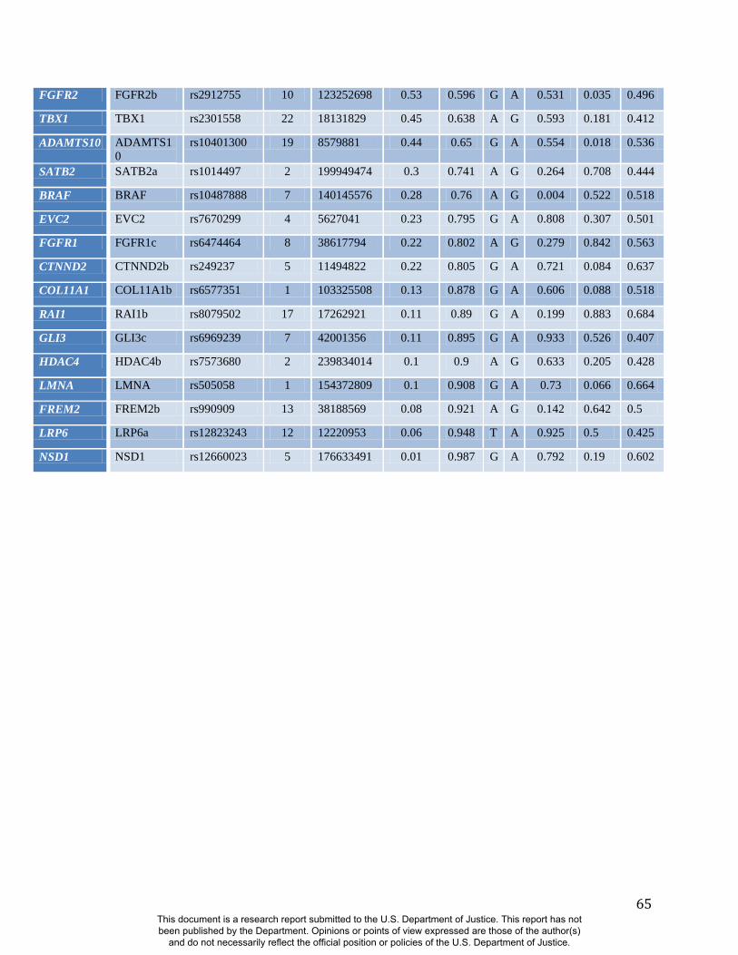
65

FGFR2 FGFR2b rs2912755 10 123252698 0.53 0.596 G A 0.531 0.035 0.496

TBX1 TBX1 rs2301558 22 18131829 0.45 0.638 A G 0.593 0.181 0.412

ADAMTS10 ADAMTS1

0

rs10401300 19 8579881 0.44 0.65 G A 0.554 0.018 0.536

SATB2 SATB2a rs1014497 2 199949474 0.3 0.741 A G 0.264 0.708 0.444

BRAF BRAF rs10487888 7 140145576 0.28 0.76 A G 0.004 0.522 0.518

EVC2 EVC2 rs7670299 4 5627041 0.23 0.795 G A 0.808 0.307 0.501

FGFR1 FGFR1c rs6474464 8 38617794 0.22 0.802 A G 0.279 0.842 0.563

CTNND2 CTNND2b rs249237 5 11494822 0.22 0.805 G A 0.721 0.084 0.637

COL11A1 COL11A1b rs6577351 1 103325508 0.13 0.878 G A 0.606 0.088 0.518

RAI1 RAI1b rs8079502 17 17262921 0.11 0.89 G A 0.199 0.883 0.684

GLI3 GLI3c rs6969239 7 42001356 0.11 0.895 G A 0.933 0.526 0.407

HDAC4 HDAC4b rs7573680 2 239834014 0.1 0.9 A G 0.633 0.205 0.428

LMNA LMNA rs505058 1 154372809 0.1 0.908 G A 0.73 0.066 0.664

FREM2 FREM2b rs990909 13 38188569 0.08 0.921 A G 0.142 0.642 0.5

LRP6 LRP6a rs12823243 12 12220953 0.06 0.948 T A 0.925 0.5 0.425

NSD1 NSD1 rs12660023 5 176633491 0.01 0.987 G A 0.792 0.19 0.602



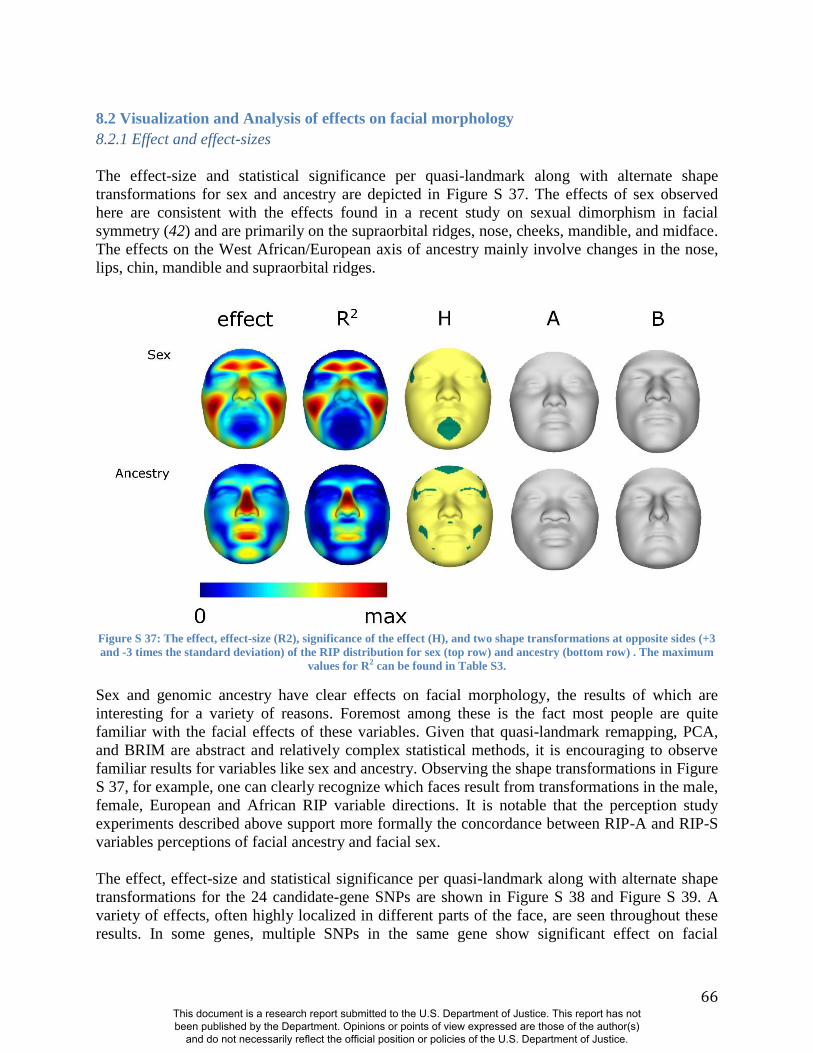
66

8.2 Visualization and Analysis of effects on facial morphology

8.2.1 Effect and effect-sizes

The effect-size and statistical significance per quasi-landmark along with alternate shape

transformations for sex and ancestry are depicted in Figure S 37. The effects of sex observed

here are consistent with the effects found in a recent study on sexual dimorphism in facial

symmetry (42) and are primarily on the supraorbital ridges, nose, cheeks, mandible, and midface.

The effects on the West African/European axis of ancestry mainly involve changes in the nose,

lips, chin, mandible and supraorbital ridges.

Figure S 37: The effect, effect-size (R2), significance of the effect (H), and two shape transformations at opposite sides (+3

and -3 times the standard deviation) of the RIP distribution for sex (top row) and ancestry (bottom row) . The maximum

values for R2 can be found in Table S3.

Sex and genomic ancestry have clear effects on facial morphology, the results of which are

interesting for a variety of reasons. Foremost among these is the fact most people are quite

familiar with the facial effects of these variables. Given that quasi-landmark remapping, PCA,

and BRIM are abstract and relatively complex statistical methods, it is encouraging to observe

familiar results for variables like sex and ancestry. Observing the shape transformations in Figure

S 37, for example, one can clearly recognize which faces result from transformations in the male,

female, European and African RIP variable directions. It is notable that the perception study

experiments described above support more formally the concordance between RIP-A and RIP-S

variables perceptions of facial ancestry and facial sex.

The effect, effect-size and statistical significance per quasi-landmark along with alternate shape

transformations for the 24 candidate-gene SNPs are shown in Figure S 38 and Figure S 39. A

variety of effects, often highly localized in different parts of the face, are seen throughout these

results. In some genes, multiple SNPs in the same gene show significant effect on facial



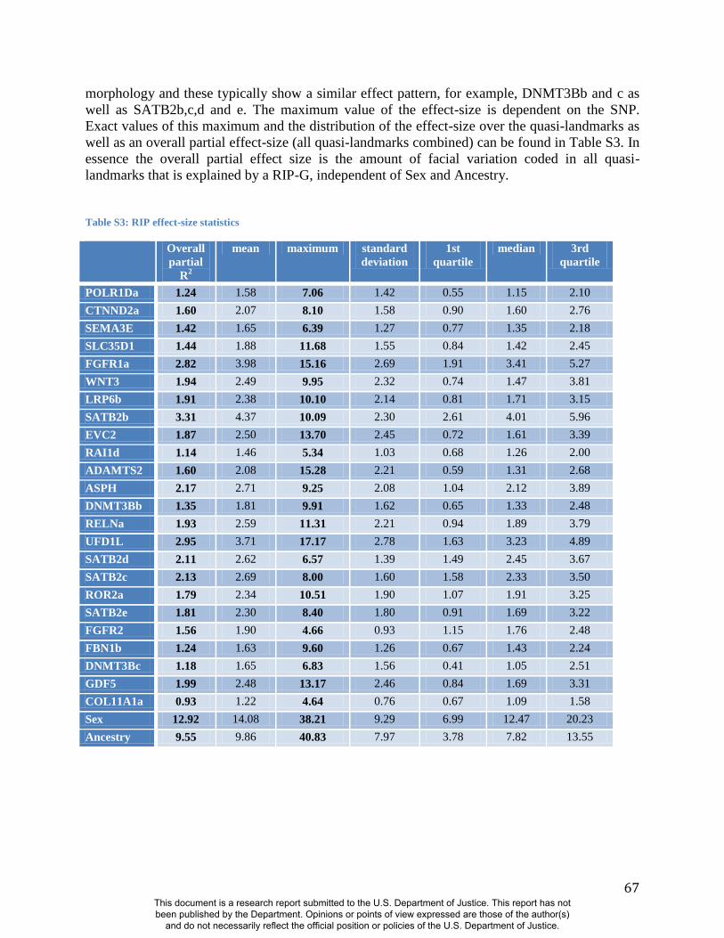
67

morphology and these typically show a similar effect pattern, for example, DNMT3Bb and c as

well as SATB2b,c,d and e. The maximum value of the effect-size is dependent on the SNP.

Exact values of this maximum and the distribution of the effect-size over the quasi-landmarks as

well as an overall partial effect-size (all quasi-landmarks combined) can be found in Table S3. In

essence the overall partial effect size is the amount of facial variation coded in all quasi-

landmarks that is explained by a RIP-G, independent of Sex and Ancestry.

Table S3: RIP effect-size statistics

Overall

partial

R2

mean maximum standard

deviation

1st

quartile

median 3rd

quartile

POLR1Da 1.24 1.58 7.06 1.42 0.55 1.15 2.10

CTNND2a 1.60 2.07 8.10 1.58 0.90 1.60 2.76

SEMA3E 1.42 1.65 6.39 1.27 0.77 1.35 2.18

SLC35D1 1.44 1.88 11.68 1.55 0.84 1.42 2.45

FGFR1a 2.82 3.98 15.16 2.69 1.91 3.41 5.27

WNT3 1.94 2.49 9.95 2.32 0.74 1.47 3.81

LRP6b 1.91 2.38 10.10 2.14 0.81 1.71 3.15

SATB2b 3.31 4.37 10.09 2.30 2.61 4.01 5.96

EVC2 1.87 2.50 13.70 2.45 0.72 1.61 3.39

RAI1d 1.14 1.46 5.34 1.03 0.68 1.26 2.00

ADAMTS2 1.60 2.08 15.28 2.21 0.59 1.31 2.68

ASPH 2.17 2.71 9.25 2.08 1.04 2.12 3.89

DNMT3Bb 1.35 1.81 9.91 1.62 0.65 1.33 2.48

RELNa 1.93 2.59 11.31 2.21 0.94 1.89 3.79

UFD1L 2.95 3.71 17.17 2.78 1.63 3.23 4.89

SATB2d 2.11 2.62 6.57 1.39 1.49 2.45 3.67

SATB2c 2.13 2.69 8.00 1.60 1.58 2.33 3.50

ROR2a 1.79 2.34 10.51 1.90 1.07 1.91 3.25

SATB2e 1.81 2.30 8.40 1.80 0.91 1.69 3.22

FGFR2 1.56 1.90 4.66 0.93 1.15 1.76 2.48

FBN1b 1.24 1.63 9.60 1.26 0.67 1.43 2.24

DNMT3Bc 1.18 1.65 6.83 1.56 0.41 1.05 2.51

GDF5 1.99 2.48 13.17 2.46 0.84 1.69 3.31

COL11A1a 0.93 1.22 4.64 0.76 0.67 1.09 1.58

Sex 12.92 14.08 38.21 9.29 6.99 12.47 20.23

Ancestry 9.55 9.86 40.83 7.97 3.78 7.82 13.55



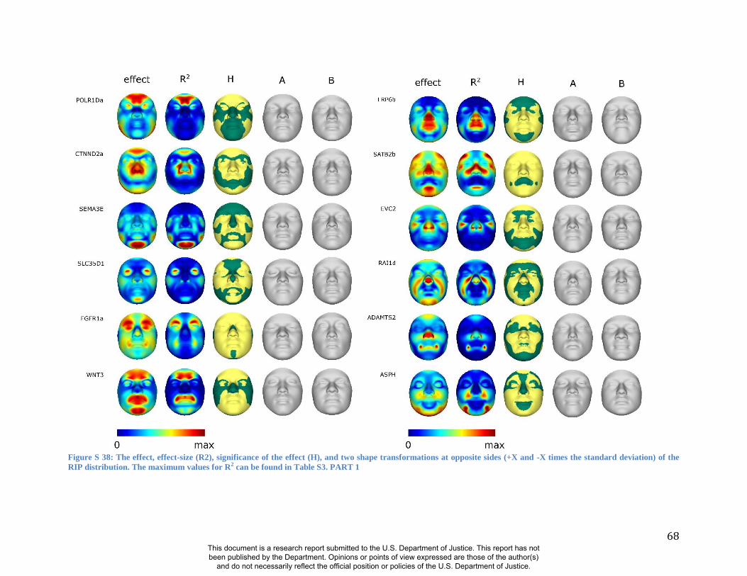
68

Figure S 38: The effect, effect-size (R2), significance of the effect (H), and two shape transformations at opposite sides (+X and -X times the standard deviation) of the

RIP distribution. The maximum values for R2 can be found in Table S3. PART 1



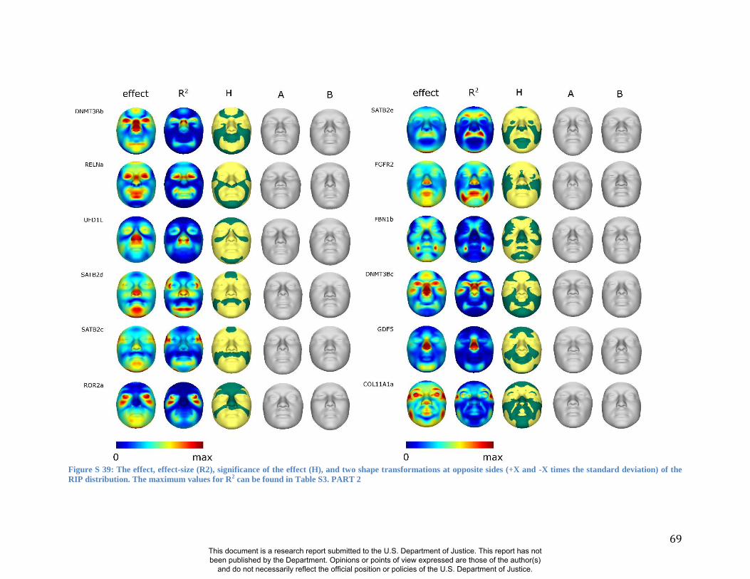
69

Figure S 39: The effect, effect-size (R2), significance of the effect (H), and two shape transformations at opposite sides (+X and -X times the standard deviation) of the

RIP distribution. The maximum values for R2 can be found in Table S3. PART 2



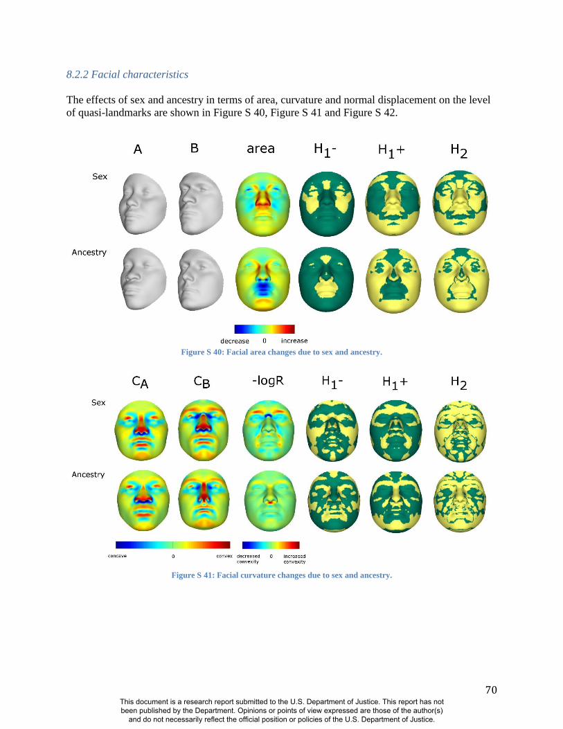
70

8.2.2 Facial characteristics

The effects of sex and ancestry in terms of area, curvature and normal displacement on the level

of quasi-landmarks are shown in Figure S 40, Figure S 41 and Figure S 42.

Figure S 40: Facial area changes due to sex and ancestry.

Figure S 41: Facial curvature changes due to sex and ancestry.



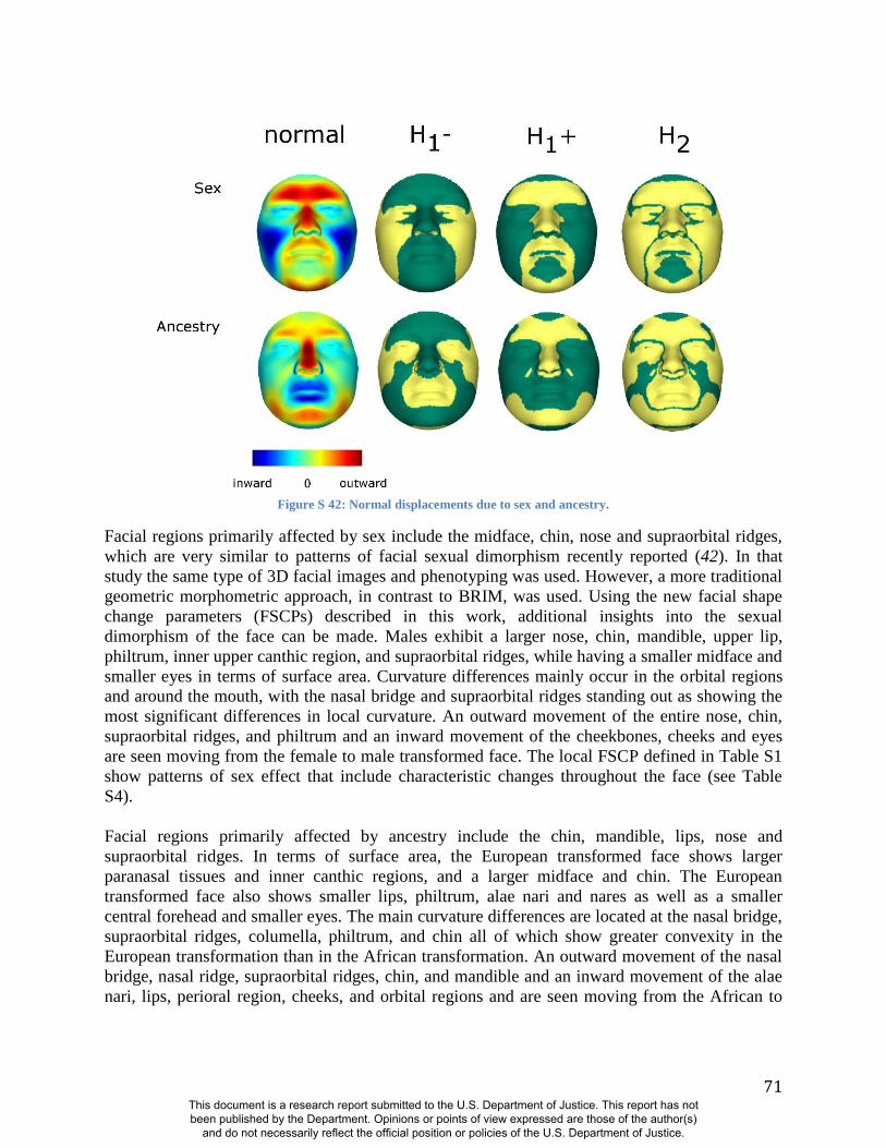
71

Figure S 42: Normal displacements due to sex and ancestry.

Facial regions primarily affected by sex include the midface, chin, nose and supraorbital ridges,

which are very similar to patterns of facial sexual dimorphism recently reported (42). In that

study the same type of 3D facial images and phenotyping was used. However, a more traditional

geometric morphometric approach, in contrast to BRIM, was used. Using the new facial shape

change parameters (FSCPs) described in this work, additional insights into the sexual

dimorphism of the face can be made. Males exhibit a larger nose, chin, mandible, upper lip,

philtrum, inner upper canthic region, and supraorbital ridges, while having a smaller midface and

smaller eyes in terms of surface area. Curvature differences mainly occur in the orbital regions

and around the mouth, with the nasal bridge and supraorbital ridges standing out as showing the

most significant differences in local curvature. An outward movement of the entire nose, chin,

supraorbital ridges, and philtrum and an inward movement of the cheekbones, cheeks and eyes

are seen moving from the female to male transformed face. The local FSCP defined in Table S1

show patterns of sex effect that include characteristic changes throughout the face (see Table

S4).

Facial regions primarily affected by ancestry include the chin, mandible, lips, nose and

supraorbital ridges. In terms of surface area, the European transformed face shows larger

paranasal tissues and inner canthic regions, and a larger midface and chin. The European

transformed face also shows smaller lips, philtrum, alae nari and nares as well as a smaller

central forehead and smaller eyes. The main curvature differences are located at the nasal bridge,

supraorbital ridges, columella, philtrum, and chin all of which show greater convexity in the

European transformation than in the African transformation. An outward movement of the nasal

bridge, nasal ridge, supraorbital ridges, chin, and mandible and an inward movement of the alae

nari, lips, perioral region, cheeks, and orbital regions and are seen moving from the African to



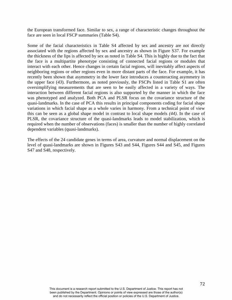
72

the European transformed face. Similar to sex, a range of characteristic changes throughout the

face are seen in local FSCP summaries (Table S4).

Some of the facial characteristics in Table S4 affected by sex and ancestry are not directly

associated with the regions affected by sex and ancestry as shown in Figure S37. For example

the thickness of the lips is affected by sex as noted in Table S4. This is highly due to the fact that

the face is a multipartite phenotype consisting of connected facial regions or modules that

interact with each other. Hence changes in certain facial regions, will inevitably affect aspects of

neighboring regions or other regions even in more distant parts of the face. For example, it has

recently been shown that asymmetry in the lower face introduces a counteracting asymmetry in

the upper face (43). Furthermore, as noted previously, the FSCPs listed in Table S1 are often

oversimplifying measurements that are seen to be easily affected in a variety of ways. The

interaction between different facial regions is also supported by the manner in which the face

was phenotyped and analyzed. Both PCA and PLSR focus on the covariance structure of the

quasi-landmarks. In the case of PCA this results in principal components coding for facial shape

variations in which facial shape as a whole varies in harmony. From a technical point of view

this can be seen as a global shape model in contrast to local shape models (44). In the case of

PLSR, the covariance structure of the quasi-landmarks leads to model stabilization, which is

required when the number of observations (faces) is smaller than the number of highly correlated

dependent variables (quasi-landmarks).

The effects of the 24 candidate genes in terms of area, curvature and normal displacement on the

level of quasi-landmarks are shown in Figures S43 and S44, Figures S44 and S45, and Figures

S47 and S48, respectively.



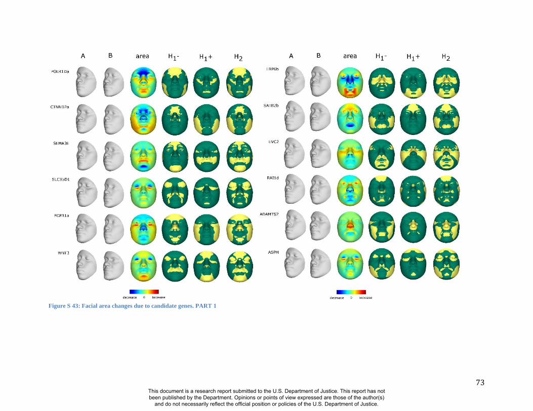
73

Figure S 43: Facial area changes due to candidate genes. PART 1



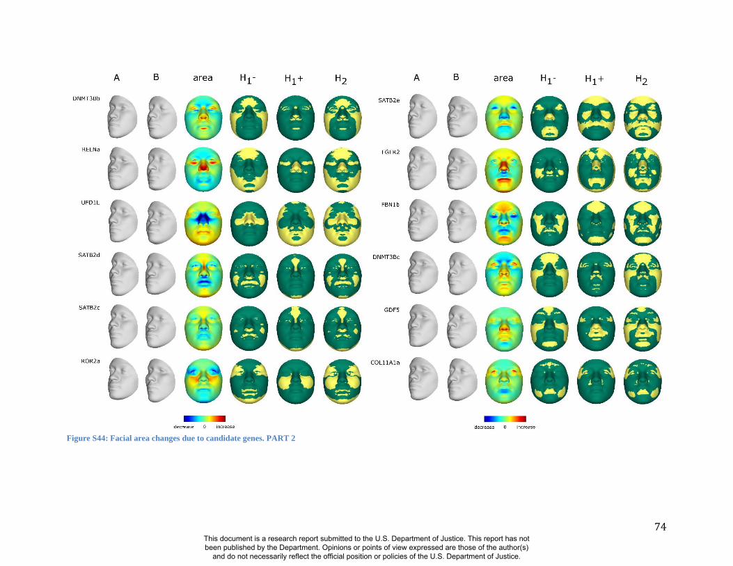
74

Figure S44: Facial area changes due to candidate genes. PART 2



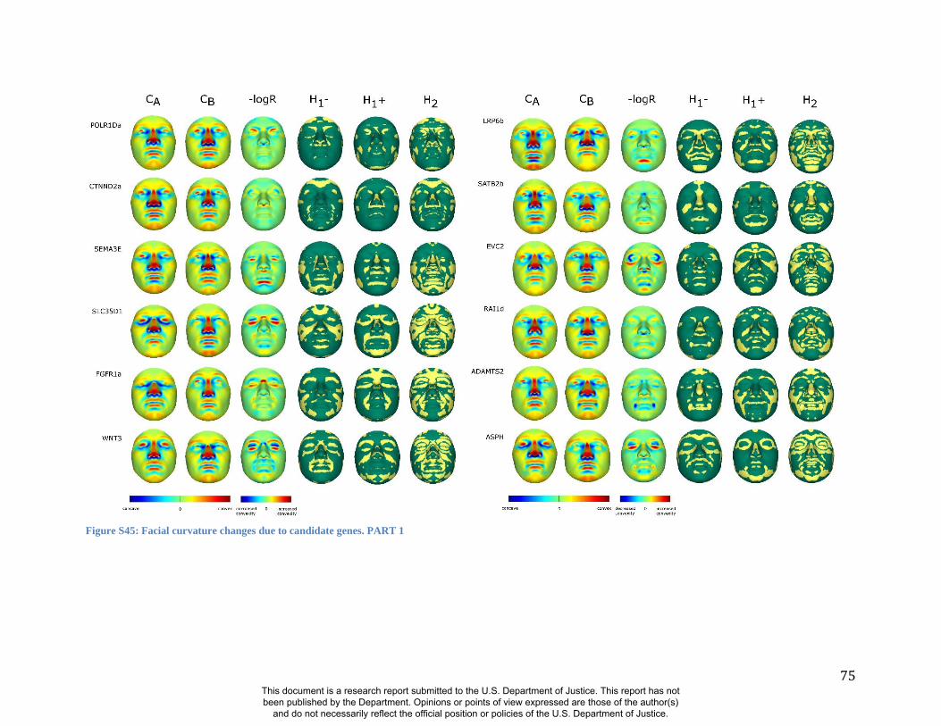
75

Figure S45: Facial curvature changes due to candidate genes. PART 1



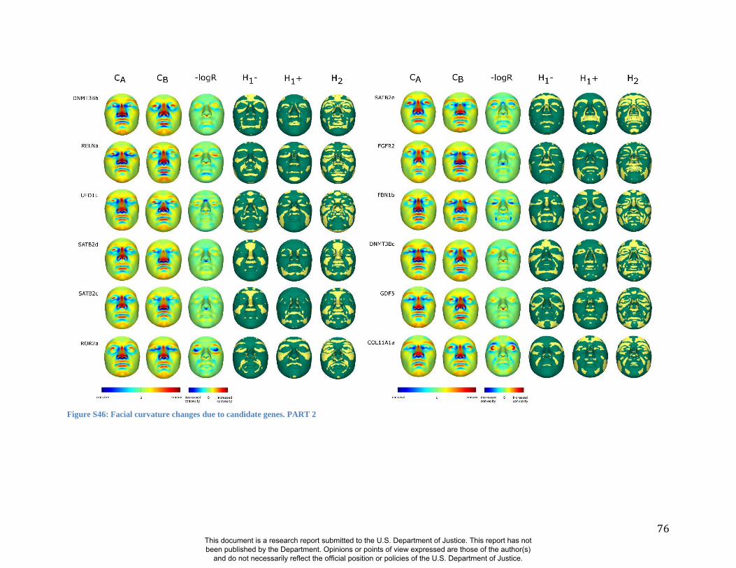
76

Figure S46: Facial curvature changes due to candidate genes. PART 2



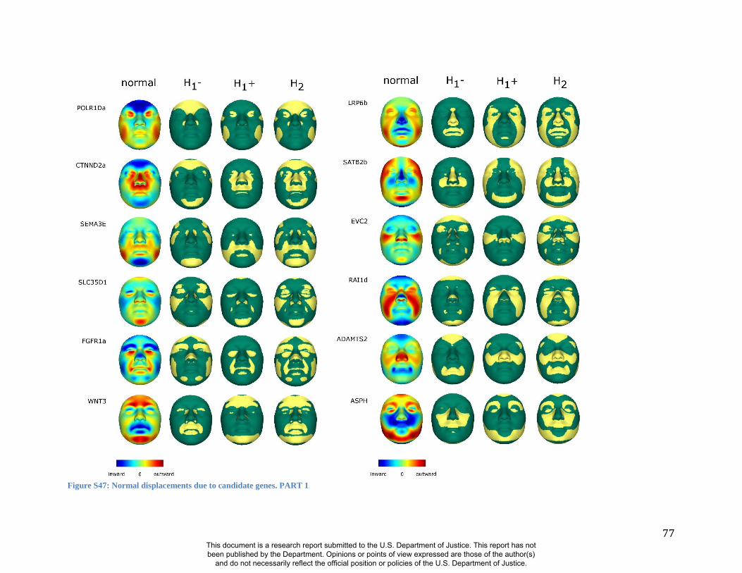
77

Figure S47: Normal displacements due to candidate genes. PART 1



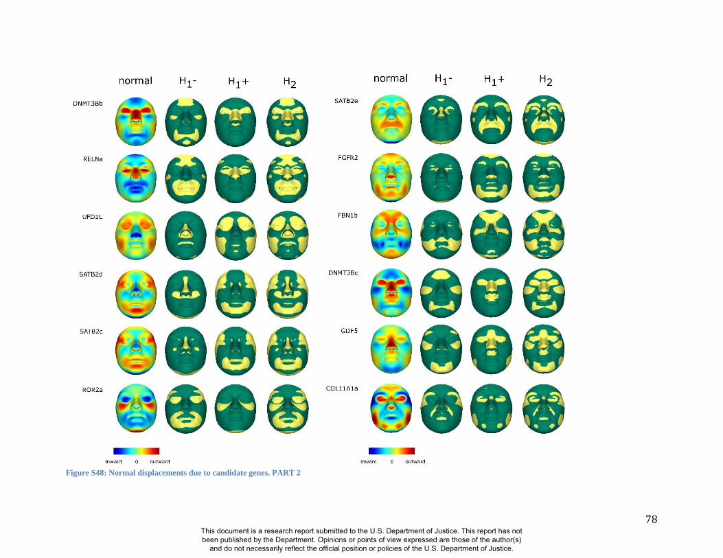
78

Figure S48: Normal displacements due to candidate genes. PART 2



79

SEMA3E

WNT3

POLR1Da

CTN

ND2a

SLC35D1

LRP6b

FGFR1a

DNMT3Bb

DNMT3Bc

ADAMTS2

RAI1d

UFD

1L

SATB2b

SATB2c

SATB2d

SATB2e

RELNa

ASPH

FGFR2

COL11A1a

EVC2

FBN1b

ROR2a

GDF5

Sex

Ancestry

Malar Flattening A 0,216 0,511 0,850 0,493 0,000 0,003 0,001 0,332 0,000 0,000 0,000 0,002 0,001 0,000 0,000 0,538 0,001 0,000 0,628 0,611 0,000 0,000 0,000 0,000 0,000 0,048

B 0,000 0,001 0,000 0,000 0,005 0,030 0,000 0,222 0,010 0,819 0,000 0,652 0,000 0,458 0,001 0,266 0,014 0,069 0,635 0,273 0,079 0,697 0,002 0,002 0,122 0,000

C 0,027 0,538 0,001 0,002 0,501 0,981 0,000 0,000 0,000 0,000 0,001 0,002 0,000 0,000 0,000 0,684 0,841 0,000 0,343 0,000 0,000 0,000 0,000 0,000 0,370 0,004

Face square/round A 0,046 0,001 0,057 0,021 0,090 0,000 0,271 0,556 0,002 0,000 0,727 0,000 0,075 0,000 0,830 0,000 0,000 0,000 0,001 0,000 0,048 0,003 0,008 0,050 0,146 0,000

Micrognathi A 0,000 0,000 0,426 0,000 0,000 0,754 0,110 0,000 0,379 0,257 0,000 0,860 0,000 0,002 0,000 0,376 0,041 0,000 0,010 0,219 0,550 0,001 0,045 0,000 0,000 0,000

B 0,000 0,000 0,173 0,839 0,113 0,000 0,000 0,490 0,004 0,701 0,017 0,000 0,640 0,103 0,030 0,002 0,014 0,277 0,005 0,648 0,001 0,000 0,000 0,000 0,000 0,000

C 0,000 0,000 0,228 0,640 0,022 0,000 0,241 0,552 0,867 0,167 0,011 0,100 0,157 0,326 0,191 0,000 0,001 0,112 0,155 0,003 0,000 0,000 0,013 0,003 0,000 0,000

Microcephaly A 0,000 0,095 0,136 0,135 0,482 0,083 0,000 0,000 0,000 0,000 0,213 0,930 0,000 0,000 0,000 0,001 0,000 0,862 0,130 0,000 0,000 0,786 0,016 0,001 0,000 0,470

B 0,205 0,000 0,000 0,000 0,456 0,772 0,000 0,001 0,010 0,000 0,000 0,186 0,000 0,070 0,008 0,176 0,002 0,005 0,002 0,262 0,000 0,001 0,110 0,915 0,000 0,000

Midface retrusion A 0,455 0,029 0,067 0,000 0,009 0,214 0,057 0,303 0,139 0,000 0,000 0,241 0,074 0,564 0,166 0,001 0,502 0,000 0,232 0,077 0,000 0,358 0,002 0,157 0,000 0,000

/ flat midface B 0,000 0,676 0,050 0,285 0,460 0,704 0,002 0,000 0,000 0,003 0,001 0,000 0,242 0,123 0,815 0,000 0,000 0,000 0,019 0,000 0,000 0,000 0,000 0,000 0,000 0,000

Frontal bossing A 0,000 0,298 0,028 0,016 0,073 0,468 0,001 0,000 0,000 0,000 0,439 0,105 0,000 0,000 0,000 0,001 0,000 0,145 0,010 0,014 0,006 0,262 0,064 0,000 0,031 0,291

Metopic ridge prominent A 0,007 0,781 0,022 0,000 0,509 0,025 0,000 0,000 0,000 0,000 0,089 0,000 0,000 0,001 0,000 0,000 0,219 0,911 0,200 0,001 0,000 0,012 0,001 0,003 0,000 0,000

Face long A 0,927 0,004 0,064 0,048 0,001 0,645 0,000 0,042 0,628 0,089 0,149 0,001 0,000 0,000 0,000 0,000 0,003 0,000 0,000 0,783 0,171 0,268 0,001 0,071 0,000 0,058

Forehead short A 0,933 0,919 0,770 0,004 0,011 0,952 0,000 0,234 0,384 0,075 0,003 0,004 0,000 0,182 0,374 0,004 0,000 0,004 0,004 0,015 0,000 0,552 0,457 0,770 0,000 0,008

Supraorbital ridge A 0,023 0,000 0,000 0,006 0,000 0,046 0,000 0,622 0,005 0,012 0,358 0,000 0,000 0,000 0,000 0,000 0,380 0,000 0,000 0,000 0,020 0,024 0,001 0,109 0,000 0,000

underdeveloped B 0,111 0,000 0,002 0,246 0,002 0,000 0,000 0,217 0,428 0,964 0,191 0,000 0,000 0,188 0,002 0,234 0,752 0,000 0,055 0,000 0,000 0,010 0,001 0,239 0,000 0,000

Forehead sloping A 0,205 0,000 0,000 0,000 0,456 0,772 0,000 0,001 0,010 0,000 0,000 0,186 0,000 0,070 0,008 0,176 0,002 0,005 0,002 0,262 0,000 0,001 0,110 0,915 0,000 0,000

B 0,738 0,263 0,021 0,282 0,000 0,826 0,000 0,007 0,624 0,010 0,000 0,874 0,037 0,000 0,000 0,001 0,000 0,000 0,000 0,016 0,000 0,000 0,004 0,000 0,000 0,000

Forehead broad/narrow A 0,001 0,000 0,000 0,000 0,029 0,004 0,000 0,203 0,520 0,006 0,687 0,280 0,000 0,000 0,000 0,000 0,001 0,024 0,014 0,059 0,967 0,006 0,082 0,163 0,959 0,120

Shallow orbits A 0,001 0,000 0,042 0,029 0,000 0,007 0,000 0,574 0,000 0,000 0,993 0,000 0,000 0,000 0,000 0,000 0,225 0,004 0,001 0,000 0,022 0,040 0,558 0,000 0,000 0,000

B 0,023 0,000 0,000 0,008 0,000 0,048 0,000 0,638 0,006 0,013 0,368 0,000 0,000 0,000 0,000 0,000 0,380 0,000 0,000 0,000 0,020 0,026 0,001 0,113 0,000 0,000

C 0,003 0,825 0,048 0,992 0,000 0,001 0,380 0,021 0,000 0,001 0,014 0,794 0,000 0,296 0,212 0,086 0,035 0,004 0,595 0,000 0,000 0,022 0,000 0,000 0,000 0,000

D 0,555 0,005 0,188 0,001 0,011 0,465 0,831 0,000 0,000 0,000 0,144 0,011 0,539 0,059 0,009 0,000 0,000 0,091 0,037 0,000 0,000 0,617 0,000 0,000 0,000 0,000

E 0,354 0,000 0,011 0,004 0,757 0,161 0,503 0,000 0,000 0,000 0,503 0,337 0,510 0,279 0,020 0,000 0,002 0,001 0,067 0,000 0,000 0,439 0,001 0,000 0,000 0,000

F 0,003 0,017 0,010 0,982 0,000 0,965 0,772 0,257 0,000 0,180 0,903 0,000 0,090 0,001 0,025 0,491 0,000 0,001 0,155 0,000 0,000 0,373 0,000 0,000 0,000 0,125

Superiorly oriented orbits A 0,000 0,000 0,592 0,773 0,000 0,000 0,000 0,002 0,433 0,087 0,139 0,281 0,415 0,038 0,270 0,000 0,000 0,000 0,900 0,863 0,939 0,001 0,001 0,633 0,062 0,006

B 0,002 0,000 0,287 0,171 0,000 0,024 0,000 0,000 0,001 0,145 0,537 0,852 0,020 0,287 0,372 0,038 0,000 0,000 0,432 0,541 0,001 0,273 0,566 0,027 0,800 0,148

C 0,001 0,000 0,660 0,887 0,000 0,000 0,019 0,000 0,014 0,194 0,075 0,638 0,116 0,038 0,084 0,000 0,001 0,000 0,855 0,265 0,034 0,023 0,280 0,051 0,714 0,363

Palpebral fissures A 0,009 0,000 0,068 0,001 0,052 0,000 0,966 0,000 0,000 0,026 0,000 0,284 0,006 0,087 0,248 0,000 0,000 0,001 0,004 0,000 0,000 0,540 0,139 0,000 0,000 0,007

downslanted B 0,043 0,000 0,014 0,002 0,024 0,000 0,105 0,000 0,000 0,029 0,000 0,067 0,007 0,080 0,148 0,000 0,000 0,000 0,012 0,000 0,000 0,992 0,020 0,000 0,000 0,272

Eyes widely spaced A 0,000 0,000 0,000 0,000 0,279 0,037 0,000 0,393 0,022 0,000 0,237 0,000 0,000 0,000 0,000 0,000 0,155 0,217 0,000 0,064 0,269 0,000 0,001 0,077 0,000 0,000

B 0,000 0,815 0,014 0,000 0,061 0,251 0,000 0,385 0,049 0,000 0,404 0,003 0,000 0,000 0,000 0,000 0,420 0,131 0,001 0,432 0,257 0,009 0,000 0,560 0,000 0,000

C 0,000 0,023 0,000 0,000 0,815 0,034 0,000 0,376 0,013 0,000 0,292 0,000 0,000 0,000 0,000 0,000 0,627 0,492 0,000 0,035 0,283 0,000 0,006 0,054 0,000 0,000

Proptosis A 0,640 0,080 0,000 0,001 0,947 0,000 0,000 0,000 0,000 0,113 0,000 0,000 0,985 0,383 0,043 0,000 0,000 0,004 0,002 0,000 0,000 0,139 0,000 0,000 0,000 0,000

B 0,589 0,101 0,000 0,495 0,894 0,000 0,000 0,000 0,000 0,288 0,000 0,000 0,119 0,007 0,000 0,000 0,000 0,097 0,026 0,000 0,000 0,438 0,000 0,000 0,000 0,000

C 0,387 0,133 0,000 0,000 0,951 0,000 0,000 0,000 0,000 0,066 0,000 0,000 0,190 0,441 0,446 0,000 0,000 0,000 0,001 0,000 0,002 0,174 0,000 0,000 0,000 0,000

D 0,468 0,002 0,000 0,010 0,000 0,000 0,000 0,000 0,000 0,214 0,000 0,000 0,522 0,611 0,039 0,000 0,000 0,069 0,001 0,000 0,000 0,209 0,000 0,000 0,000 0,000

E 0,142 0,992 0,000 0,000 0,001 0,001 0,000 0,001 0,000 0,090 0,000 0,000 0,598 0,192 0,039 0,008 0,000 0,000 0,005 0,000 0,010 0,112 0,000 0,000 0,000 0,000

F 0 0 0,091 0,009 0,000 0,002 0,000 0,000 0,000 0,264 0,793 0,702 0,041 0,123 0,626 0,000 0,000 0,000 0,835 0,950 0,000 0,359 0,276 0,238 0,000 0,097

Nasal ridge narrow A 0,000 0,045 0,458 0,000 0,010 0,409 0,000 0,000 0,654 0,000 0,438 0,000 0,000 0,000 0,000 0,033 0,725 0,122 0,000 0,019 0,041 0,000 0,266 0,002 0,000 0,000

B 0,000 0,000 0,278 0,034 0,000 0,002 0,042 0,000 0,066 0,000 0,000 0,001 0,000 0,000 0,000 0,000 0,005 0,000 0,413 0,266 0,042 0,000 0,509 0,003 0,219 0,000

C 0,000 0,194 0,771 0,000 0,000 0,000 0,003 0,058 0,312 0,000 0,002 0,530 0,000 0,000 0,000 0,000 0,020 0,000 0,052 0,020 0,049 0,000 0,436 0,003 0,000 0,000

D 0,000 0,000 0,113 0,401 0,000 0,645 0,602 0,000 0,000 0,147 0,000 0,000 0,002 0,000 0,000 0,000 0,014 0,000 0,647 0,764 0,132 0,000 0,052 0,029 0,079 0,000

Nasal ridge retruded A 0,194 0,819 0,488 0,000 0,078 0,000 0,004 0,000 0,000 0,001 0,531 0,000 0,000 0,000 0,000 0,000 0,000 0,784 0,769 0,059 0,075 0,361 0,155 0,000 0,000 0,000

Nasal bridge depressed A 0,088 0,857 0,000 0,040 0,728 0,000 0,514 0,000 0,000 0,024 0,033 0,012 0,000 0,001 0,000 0,001 0,001 0,939 0,128 0,001 0,006 0,000 0,097 0,000 0,000 0,000

Nasal bridge wide A 0,024 0,000 0,033 0,179 0,000 0,000 0,000 0,411 0,080 0,000 0,023 0,000 0,000 0,000 0,000 0,000 0,035 0,043 0,001 0,006 0,032 0,000 0,351 0,035 0,000 0,000

B 0,000 0,646 0,000 0,000 0,601 0,963 0,000 0,000 0,101 0,038 0,570 0,543 0,000 0,000 0,000 0,000 0,003 0,000 0,798 0,025 0,000 0,000 0,012 0,011 0,063 0,946

Nose wide A 0,099 0,128 0,799 0,010 0,935 0,000 0,000 0,882 0,551 0,000 0,312 0,130 0,000 0,262 0,131 0,040 0,000 0,000 0,007 0,000 0,002 0,000 0,001 0,061 0,000 0,000

B 0,347 0,018 0,574 0,000 0,546 0,001 0,000 0,933 0,389 0,000 0,321 0,248 0,000 0,756 0,012 0,990 0,100 0,001 0,000 0,000 0,000 0,000 0,000 0,998 0,000 0,000

Nose snubbed A 0,199 0,013 0,000 0,000 0,149 0,002 0,117 0,000 0,000 0,000 0,000 0,125 0,000 0,000 0,000 0,000 0,000 0,083 0,000 0,378 0,023 0,000 0,171 0,000 0,221 0,000

Nares anteverted A 0,552 0,028 0,069 0,000 0,846 0,000 0,553 0,000 0,000 0,018 0,000 0,168 0,000 0,000 0,000 0,000 0,000 0,204 0,000 0,515 0,170 0,000 0,016 0,000 0,015 0,000

Cleft lip A 0,000 0,000 0,240 0,129 0,042 0,023 0,087 0,028 0,001 0,000 0,009 0,051 0,477 0,002 0,001 0,011 0,955 0,000 0,000 0,695 0,000 0,183 0,586 0,000 0,000 0,000

B 0,000 0,000 0,601 0,000 0,486 0,001 0,105 0,002 0,000 0,001 0,312 0,588 0,002 0,309 0,000 0,000 0,000 0,000 0,061 0,031 0,029 0,004 0,005 0,000 0,000 0,000

C 0,000 0,000 0,042 0,002 0,060 0,113 0,013 0,006 0,000 0,095 0,743 0,000 0,023 0,000 0,000 0,000 0,363 0,000 0,000 0,000 0,000 0,039 0,017 0,000 0,000 0,000

D 0,618 0,396 0,170 0,013 0,511 0,000 0,000 0,027 0,015 0,000 0,070 0,000 0,568 0,291 0,757 0,000 0,000 0,248 0,000 0,757 0,358 0,673 0,680 0,000 0,000 0,091

E 0,565 0,776 0,553 0,000 0,781 0,000 0,000 0,000 0,000 0,000 0,827 0,000 0,000 0,008 0,002 0,308 0,000 0,116 0,004 0,986 0,087 0,393 0,996 0,000 0,000 0,000

F 0,191 0,000 0,000 0,000 0,737 0,000 0,111 0,000 0,000 0,126 0,000 0,537 0,000 0,000 0,000 0,000 0,007 0,000 0,000 0,980 0,681 0,230 0,005 0,000 0,000 0,000

Mouth wide A 0,995 0,033 0,001 0,146 0,826 0,881 0,000 0,418 0,377 0,028 0,354 0,015 0,001 0,000 0,000 0,658 0,000 0,000 0,002 0,751 0,000 0,035 0,000 0,178 0,076 0,000

Upper vermilion thick A 0,000 0,000 0,886 0,677 0,082 0,034 0,333 0,961 0,273 0,087 0,151 0,028 0,008 0,001 0,000 0,000 0,148 0,002 0,146 0,447 0,047 0,000 0,495 0,000 0,000 0,000

Lower vermilion thick A 0,895 0,540 0,036 0,981 0,421 0,756 0,012 0,668 0,753 0,000 0,016 0,000 0,000 0,053 0,145 0,000 0,063 0,244 0,000 0,000 0,004 0,028 0,000 0,039 0,216 0,000

Lips thick A 0,000 0,005 0,253 0,837 0,121 0,318 0,052 0,838 0,433 0,034 0,021 0,000 0,000 0,001 0,000 0,869 0,052 0,217 0,017 0,010 0,004 0,000 0,074 0,074 0,000 0,000

Maxilla prominent A 0,005 0,079 0,307 0,000 0,269 0,003 0,000 0,054 0,014 0,004 0,000 0,023 0,000 0,011 0,000 0,086 0,972 0,000 0,055 0,441 0,000 0,506 0,004 0,001 0,000 0,294

B 0,027 0,538 0,001 0,002 0,501 0,981 0,000 0,000 0,000 0,000 0,001 0,002 0,000 0,000 0,000 0,684 0,841 0,000 0,343 0,000 0,000 0,000 0,000 0,000 0,370 0,004

Philtrum long A 0,000 0,000 0,105 0,976 0,832 0,000 0,015 0,147 0,243 0,591 0,003 0,676 0,018 0,000 0,000 0,037 0,841 0,002 0,000 0,810 0,052 0,746 0,000 0,000 0,000 0,000

Sunken cheeks A 0,087 0,422 0,000 0,000 0,892 0,276 0,000 0,000 0,000 0,000 0,653 0,000 0,000 0,359 0,007 0,000 0,000 0,000 0,874 0,001 0,001 0,282 0,151 0,001 0,000 0,000

Eyes large A 0,256 0,000 0,591 0,005 0,000 0,055 0,000 0,131 0,010 0,017 0,033 0,956 0,171 0,470 0,234 0,000 0,000 0,577 0,696 0,000 0,658 0,002 0,000 0,008 0,000 0,005

B 0,700 0,166 0,469 0,018 0,001 0,000 0,000 0,281 0,363 0,147 0,568 0,004 0,100 0,150 0,951 0,723 0,000 0,000 0,020 0,000 0,448 0,000 0,000 0,055 0,000 0,200

Nasal tip large A 0,206 0,074 0,291 0,018 0,247 0,000 0,000 0,006 0,004 0,000 0,439 0,000 0,363 0,482 0,481 0,000 0,000 0,101 0,000 0,318 0,478 0,332 0,849 0,000 0,000 0,019

B 0,330 0,096 0,269 0,083 0,745 0,000 0,000 0,009 0,013 0,000 0,489 0,000 0,957 0,594 0,015 0,000 0,000 0,125 0,000 0,579 0,536 0,709 0,646 0,000 0,000 0,000

C 0,110 0,233 0,542 0,000 0,738 0,000 0,000 0,000 0,000 0,000 0,082 0,000 0,000 0,001 0,000 0,014 0,000 0,880 0,001 0,465 0,011 0,308 0,992 0,000 0,000 0,000

Table S 4: P-values under 10,000 permutations for the local FSCPs listed in TableS1 tested for the 24 candidate genes, sex and ancestry. Green cell, significant (p<0.05) effect. Yellow cell, significant effect (p<0.05). Red cell, non-significant effect (p>=0.05). White cell, non-significant effect (p>=0.05)



80

8.2.3 Comparing and contrasting facial changes in the clinical and normal range

We carefully examined the RIP-G transformations and FSCP results for the suggestive SNPs

(p<0.1) in the ANOVA test. Some striking correspondence with clinical dysmorphology reported

in the human syndromes associated with mutation of the respective genes or with relevant animal

models is observed. In the context of these observations, below we review the results of the

analysis the 24 candidate genes in the order of increasing p-value as shown in Table S2 (note that

when facial characteristic changes or effects are mentioned or noted, we refer to significant

effects and FSCPs):

- Mutations in the human RNA polymerase I subunit D (POLR1D; OMIM#613715) gene on

chromosome 13q12.2 can lead to the autosomal dominant condition Treacher-Collins

syndrome-2 (TCS2; OMIM#613717). The facial phenotype in TCS2 includes a distinctive

pattern of facial bone hypoplasia associated with bilateral downward slanting palpebral

fissures and symmetric convex facial profile resulting from hypoplasia of the zygomatic

bones. Affected persons may also manifest colobomas of the lower eyelids, and mandibular

hypoplasia.

- The normal-range results of the SNP in rs507217 in POLR1D depicted in Figure S 38

indicate strong effects in the eyes as well as the forehead and mandible. When observing the

shape transformations associated with this SNP, downward slanting palpebral fissures can be

perceived in shape transformation “B”. The curvature and the normal displacement of the

eyes are affected in Error! Reference source not found. and Error! Reference source not found. respectively and many local FSCPs related to the eyes including downward

slanted palpebral fissures are noted in Table S4. The bilateral parts of the mandible are

affected in Figure S 38 and this mainly in terms of area (Figure S 43) and normal

displacement (Error! Reference source not found.). Finally, the cheekbones are

significantly different in terms of area (Figure S 43), which also results in associated changes

like malar flattening and midface retrusion (Table S4). It is highly possible that these

characteristics are associated with differences in zygomatic bone development.

- Genomic deletions of of chromosome 5p15.2, which can include the human delta-catenin 2

(CTNN2D; OMIM#604275), result in Cri-du-chat syndrome. e. The craniofacial features of

Cri-du-chat syndrome include a round face, hypertelorism, a very wide nasal bridge,

downward slanting palpebral fissures, a wide mouth, down-turned corners of the mouth,

micrognathia and epicanthal folds.

- The normal-range effects of the SNP in rs2277054 in CTNN2D shown in Figure S 38 are

found in the midface, nose, eyes (with an emphasis on the epicanthic region), lower mandible

and forehead. Wide nasal bridge and orbital hypertelorism can be perceived in the shape

transformations and also Table S4 (eyes widely spaced). The nose in general appears to be

different in width in each of the three primary FSCPs as well as in the local FSCPs like

narrow nasal ridge, wide nose and wide nasal bridge as listed in Table S4. Other nasal

features in Table S4 are affected as well. The curvature of the nasal ridge (Error! Reference source not found.) and the normal displacement of almost the entire nose

region (Error! Reference source not found.) are significantly different. Consistent with

the results in Table S4, the normal displacement results indicate a nose that is more

prominent in the anterior-posterior plane and wider versus a narrower and more retruded



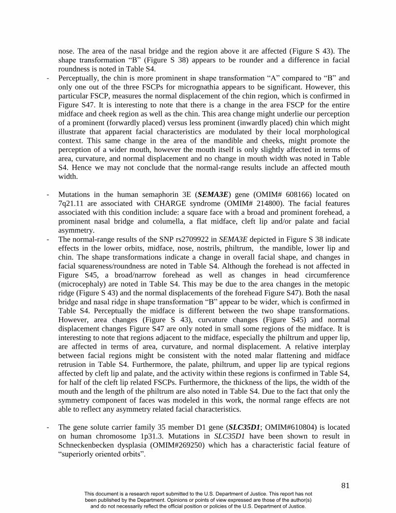
81

nose. The area of the nasal bridge and the region above it are affected (Figure S 43). The

shape transformation “B” (Figure S 38) appears to be rounder and a difference in facial

roundness is noted in Table S4.

- Perceptually, the chin is more prominent in shape transformation “A” compared to “B” and

only one out of the three FSCPs for micrognathia appears to be significant. However, this

particular FSCP, measures the normal displacement of the chin region, which is confirmed in

Figure S47. It is interesting to note that there is a change in the area FSCP for the entire

midface and cheek region as well as the chin. This area change might underlie our perception

of a prominent (forwardly placed) versus less prominent (inwardly placed) chin which might

illustrate that apparent facial characteristics are modulated by their local morphological

context. This same change in the area of the mandible and cheeks, might promote the

perception of a wider mouth, however the mouth itself is only slightly affected in terms of

area, curvature, and normal displacement and no change in mouth width was noted in Table

S4. Hence we may not conclude that the normal-range results include an affected mouth

width.

- Mutations in the human semaphorin 3E (SEMA3E) gene (OMIM# 608166) located on

7q21.11 are associated with CHARGE syndrome (OMIM# 214800). The facial features

associated with this condition include: a square face with a broad and prominent forehead, a

prominent nasal bridge and columella, a flat midface, cleft lip and/or palate and facial

asymmetry.

- The normal-range results of the SNP rs2709922 in SEMA3E depicted in Figure S 38 indicate

effects in the lower orbits, midface, nose, nostrils, philtrum, the mandible, lower lip and

chin. The shape transformations indicate a change in overall facial shape, and changes in

facial squareness/roundness are noted in Table S4. Although the forehead is not affected in

Figure S45, a broad/narrow forehead as well as changes in head circumference

(microcephaly) are noted in Table S4. This may be due to the area changes in the metopic

ridge (Figure S 43) and the normal displacements of the forehead Figure S47). Both the nasal

bridge and nasal ridge in shape transformation “B” appear to be wider, which is confirmed in

Table S4. Perceptually the midface is different between the two shape transformations.

However, area changes (Figure S 43), curvature changes (Figure S45) and normal

displacement changes Figure S47 are only noted in small some regions of the midface. It is

interesting to note that regions adjacent to the midface, especially the philtrum and upper lip,

are affected in terms of area, curvature, and normal displacement. A relative interplay

between facial regions might be consistent with the noted malar flattening and midface

retrusion in Table S4. Furthermore, the palate, philtrum, and upper lip are typical regions

affected by cleft lip and palate, and the activity within these regions is confirmed in Table S4,

for half of the cleft lip related FSCPs. Furthermore, the thickness of the lips, the width of the

mouth and the length of the philtrum are also noted in Table S4. Due to the fact that only the

symmetry component of faces was modeled in this work, the normal range effects are not

able to reflect any asymmetry related facial characteristics.

- The gene solute carrier family 35 member D1 gene (SLC35D1; OMIM#610804) is located

on human chromosome 1p31.3. Mutations in SLC35D1 have been shown to result in

Schneckenbecken dysplasia (OMIM#269250) which has a characteristic facial feature of

“superiorly oriented orbits”.



82

- The normal-range results of the SNP in rs1074265 in SLC35D1 depicted in Figure S 38

indicate strong effects at the eyes and orbital regions, as well as the midface and the chin. In

accordance with classic phenotypic descriptions of superiorly oriented orbits, one can readily

perceivea difference in the orientation of the eyes and orbits between the shape

transformations, the eyes appear to be looking downwards “A” or upwards “B”. Dividing the

eyes and orbits into upper and lower regions, we see opposite changes in terms of area

(Figure S 43), curvature (Figure S45) and normal displacement (Figure S47). Additionally,

the results of the local FSCPs measuring superiorly oriented orbits (Table S4) are consistent

with this facial characteristic . The effects in the midface and the chin are mainly changes in

terms of curvature (Figure S45) and normal displacement (Figure S47) leading to malar

flattening and along versus short face (Table S4).

- Mutations in the human fibroblast growth factor receptor 1 (FGFR1;OMIM#136350) gene

located on chromosome 8p21.23-p21.22 can result in four autosomal dominant craniofacial

disorders: Jackson-Weiss syndrome (OMIM#123150), which is characterized by

craniosynostosis and midfacial hypoplasia; trigonocephaly (OMIM#190440), which is

characterized by a keel-shaped forehead resulting in a triangle-shaped cranium when viewed

from above; osteoglophonic dysplasia (OMIM#166250), which is characterized by

craniosynostosis, a prominent supraorbital ridge, a depressed nasal bridge; and Pfeiffer

syndrome (OMIM#101600), which is characterized by midface hypoplasia, and depending

on the subtype, ocular proptosis, a short cranial base, and a cloverleaf skull.

- The normal-range results of the SNP rs13267109 in FGFR1 depicted in Figure S 38 indicate

the strongest effects in the supraorbital ridges, the forehead, the eyes, midface, nose and the

corners of the mouth. It should be noted that most of the face is significantly affected.

Perceptually, the strongest differences in the shape transformations are indeed the forehead,

supraorbital ridges and nasal bridge. Area changes (Figure S 43) occur in the forehead, nasal

tip, nasal bridge/root, midface, cheeks and the chin. The curvature changes (Figure S45) are

located in the supraorbital ridges, with opposite changes on the forehead slightly above them

(indicating prominent supraorbital ridges), and in the nasal bridge and inferior half of the

eyes, with opposite changes in the cheekbones (indicating midface hypoplasia). Normal

displacements (Figure S47) occur in the forehead, supraorbital ridges, nasal tip, paranasal

tissues and cheeks. Focusing on the forehead as one of the most prominent changing regions,

noted related FSCPs in Table S4 include microcephaly, frontal bossing, prominent metopic

ridge, forehead short/long, forehead broad/narrow, and forehead sloping. Supraorbital ridges

under/overdeveloped is also noted in Table S4. With regard to the midface, FSCPs noted in

Table S4 include malar flattening, midface retrusion/flat midface (midfacial hypolplasia) and

prominent maxilla. Finally for the nose, noted FSCPs in Table S4 include wide nasal bridge,

wide nose, large nasal tip and retruded nasal ridge. Although area and curvature changes

clearly occur in the nasal bridge and affect its appearance, the FSCP for depressed nasal

bridge is not noted in Table S4, because there was no normal displacement measured in this

region (Figure S47).

- Mutations in the human WNT 3 protein which is encoded by the WNT3 gene

(OMIM#165330) located on chromosome 17q21.31 can result in an autosomal recessive

condition, Tetra-Amelia syndrome (OMIM#273395). Infants with Tetra-Amelia are generally

stillborn or die as neonates. In addition to having no limbs or pelvis, they have many other



83

anatomical problems including numerous craniofacial anomalies: cleft lip/cleft palate,

micrognathia, microtia, single naris, prominent nose, no nose, microphthalmia, microcornea,

coloboma, and palpebral fusion. Note that many of these features are associated with the

eyes.

- The normal-range results of the SNP rs199501 in WNT3 shown in Figure S 38 indicate

effects in the eyes, forehead towards the nasal bridge, philtrum, lips, and chin. The shape

transformations are clearly distinct with several characteristic facial changes. The eyes,

similar to the results of SLC35D1, show opposite changes in area (Figure S 43), curvature

(Figure S45), and normal displacement (Figure S47) for the upper and lower parts of the

eyes, leading to a wide range of FSCPs noted in Table S4 that are related to the eyes, such as

superiorly oriented orbits, shallow orbits, palpebral fissures downslanted, eyes large and eyes

widely spaced. Similar to SEMA3E, the philtrum and upper lip are typical regions affected by

cleft lip and palate, and a strong change in terms in area (Figure S 43), curvature (Figure

S45), and normal displacement (Figure S47) is observed within these regions for the normal-

range results. Half of the cleft-lip related FSCPs are significant (Table S4). The thickness of

the lips, the width of the mouth, and the length of the philtrum are also noted in Table S4.

The chin exhibits changes in area (Figure S 43) and curvature (Figure S45) as well as normal

displacement (Figure S45) all three FSCPs for micrognathia are significant (Table S4). The

entirety of the of the nose, through the nasal bridge and toward the inferior limit of the

forehead is affected and some nose related FSCPs are noted in Table S4, such as width of the

nasal ridge and bridge, snubbed nose and anteverted nares.

- The mouse homologue of the human low density lipoprotein receptor-related protein 6

(LRP6; OMIM#603507) gene is critical for mouse lip development and bilateral cleft lip is

seen in LRP6 knockout mice (26). LRP6 is known to interact with the WNT signaling

pathway. However, no human craniofacial diseases have yet been linked to the LRP6 gene or

to the gene region on human chromosome 12p13.2.

- Observing the shape transformation in Figure S 38, a change from prominent lips with a thick

and convex vermillion to less prominent lips with a thin and more concave vermillion. This is

confirmed by looking at the normal displacement results (Figure S47). Interestingly, the lips

appear to be perfectly segmented out in the H1- significant map (Figure S47). Besides normal

displacements, some curvature changes in the lips are observed (Figure S45) and area

changes in the regions surrounding the lips (Figure S 43). All but one cleft lip related, and

several nose and eye/orbit related FSCPs are significant (Table S4).

- Mutations in the human special AT-rich sequence binding protein 2 gene (SATB2;

OMIM#608148) located on 2q33.1 can result in cleft palate with mental retardation

(OMIM#119540). Craniofacial features of deletions of the SATB2 gene include prominent

forehead, prominent nasal bridge, wide columella, micrognanthia, microcephaly, and cleft

palate (45).

- Statistically significant normal-range effects of the four (rs1357582, rs6759018, rs4530349,

and rs4673339) of the five SNPs tested in SATB2 are depicted in Figure S 38 (rs1357582)

and Figure S 39 (rs6759018, rs4530349, and rs4673339). The effects, FSCP results, and the

shape transformations of the different SNPs in SATB2 are very similar. In the shape

transformations, the shape of the nose as well as the chin and overall head and forehead are

distinctively different. All four SNPs show frontal bossing, a prominent metopic ridge,



84

forehead sloping and forehead width change (Table S4). Two out of four SNPs also exhibit a

change in forehead length. Related to the forehead, all four SNPs are significant for the

microcephaly FSCP. All four SNPs also show area and (Figure S 43-S44) curvature changes

(Figure S46) as well as normal displacements (Figure S48) in at least some part of the

forehead. All four SNPs show curvature changes (Figure S46) and normal displacements

(Figure S48) of the nasal ridge and bridge, and all but rs4673339, also show area changes

(Figure S 43-S44) in these regions. The FSCPs related to the nose (Table S4), including nasal

ridge narrow and retruded, wide nasal bridge, snubbed nose, and anteverted nares, are also

significant for all four SNPs. Some SNPs also show a large nasal tip and a wide nose,

concluding that the nose is clearly affected by this gene. The chin is alternatively affected in

terms of area, curvature, and normal displacement depending on the SNP analyzed, which is

also seen in Table S4 where different FSCPs for microganthia are noted across the four SNPs

with some overlap present. There are changes of the curvature of the philtrumfor all SNPs

and for some SNPs the normal displacement and area are altered as well. For all SNPs most

of the cleft lip and palate related FSCPs are significant.

- Mutations in the human EVC2 gene (OMIM#607261) located on chromosome 4p16.2 can

lead to the autosomal recessive condition known as Ellis-van Creveld syndrome

(OMIM#225500), which is characterized craniofacially a “partial hare-lip” (short upper lip)

or “lip-tie” (upper lip frenulum). Mutations in EVC2 can also lead to an autosomal dominant

disorder called Weyers acrofacial dysostosis (OMIM#193530), which has some facial

phenotypic overlap.

- The normal-range results of the SNP rs1001971 in EVC2 shown in Figure S 38 indicate

effects in the alae nasi, cheekbones and lateral orbits, affecting the upper lip and philtrum,

nose, orbits and the forehead and the lower chin. Perceptually, the strongest difference is

indeed located in the lower nose area, philtrum and upper lip, and additionally an overall

long/ short face difference is noted. Also notable are area changes is the region around the

lips. In fact the lips appear to be delineated in the H1- significance map (Figure S 43). The

most prominent curvature changes occur in the orbits, cheekbones and chin. An interesting

opposite change in curvature is noted in the lower and upper part of the upper lip. The normal

displacement (Figure S47) is clearly noted in the eyes, cheekbones, forehead, nares,

columella, and lower chin. A number of the FSCPs related to the orbits and forehead are

noted in Table S4. The same is true for the nose. Regarding lip variation, half of the cleft lip

and palate FSCPs are noted; thickness of the lips, mouth width, and a borderline (p=0.052)

change in philtrum length are observed.

- Deletions of human chromosome 17p11.2 and point mutations in the gene RAI1 can cause

Smith-Magenis Syndrome (SMS; OMIM#182290). The facial characteristics are perhaps best

summarized by (46):

“The facial phenotype of SMS is quite distinctive, even in the young child. The

overall face shape is broad and square. The brows are heavy, with excessive

lateral extension of the eyebrows. The eyes slant upwards and appear close set

and deep set. The nose has a depressed root and, in the young child, a scooped

bridge. With time, the bridge becomes more ski jump shaped. The height of the

nose is markedly reduced while the nasal base is broad and the tip of the nose is

full. The shape of the mouth and upper lip are most distinctive. The mouth is wide



http://www.omim.org/entry/193530

85

with full upper and lower lips. The central portion of the upper lip is fleshy and

everted with bulky philtral pillars, producing a tented appearance that, in profile,

is striking. With age, mandibular growth is greater than average and exceeds that

of the maxilla. This leads to increased jaw width and protrusion and marked

midface hypoplasia.”

- The normal-range results of the SNP rs4925108 in RAI1 depicted in Figure S 38 indicate

effects in the nasal tip and nasal bridge, eyes, midface, cheeks, chin, and the top of the

forehead. The shape transformations both frontal (Figure S 38) and lateral (Figure S 43) are

quite distinct and the most remarkable perceived differences include a ski jump shaped nose

(shape transformation “A”) with bulky philtral pillars/ridges. The eyes exhibit small area

(Figure S 43) and curvature changes (Figure S45) and more substantial normal displacement

changes (Figure S47). The FSCP for palpebral fissures downslanted (being the opposite of

slanting upwards) and proptosis (related to forward displacement of the eyes) are noted in

Table S4. The effects in the nose are clearly interesting and distinct, especially the opposite

normal displacement (Figure S47) of the nasal bridge and the area slightly above the nasal

tip, creating the appearance of an upturned nasal tip. Significant nose-related FSCPs in Table

S4 include, nasal bridge depressed and nasal bridge/ridge width (one out of two measures),

nose snubbed, and nares anteverted. The shape of the lips and mouth differ in terms of

curvature (Figure S45) and in terms of area (Figure S 43). Related FSCPs noted in Table S4

include thickness of the lips and the length of the philtrum. The midface and the cheeks are

most substantially affected in terms of normal displacement (Figure S47), and are consistent

with the significant local FSCPs in Table S4, such as malar flattening and midface

retrusion/hypoplasia.

- Mutations in the human ADAMTS2 (OMIM#604539) gene located on 5q35.3 can cause

Ehlers-Danlos syndrome, type VIIC (OMIM#225410). The facial features of Ehlers-Danlos

VIIC include epicanthal folds, a depressed nasal bridge, micrognathia, large eyes, a small

chin, sunken cheeks, a thin nose and thin lips.

- The normal-range results of the SNP rs3822601 in ADAMTS2 shown in Figure S 38 indicate

effects in midface, lower nose, and lips as well as in the nasal bridge and forehead. The most

prominent perceptual differences between both shape transformations include the width of

the nose, the size and spacing of the orbits and eyes and the shape of the lower face. Focusing

on the eyes and orbits, there are changes in orbital curvature (Figure S45) and they exhibit a

normal displacement (Figure S47). Related FSCPs noted in Table S4 include, shallow orbits,

downslanted palpebral fissures, eyes widely spaced, and one out of two FSCPs for large eyes.

The cheeks are mainly changed in terms of area (Figure S 43) and the FSCP for sunken

cheeks is significant. The nose is affected in many ways and it is one of the most striking

features of this RIP-G (Figure S 43, S45 and S47), clearly progressing from a wide to a thin

nose in the shape transformations. All nasal related FSCPs in Table S4 are noted for this SNP

including nasal bridge depressed and nose width. Area changes (Figure S43), curvature

changes (Figure S45) and normal displacements are noted for the lips or parts of the lips and

the noted related FSCPs in Table S4 including lip thickness and mouth width. Although

perceptually different in the shape transformations, the chin itself, The FSCP for

micrognathia is not significant nor is the chin region significant for the area FSCP.



86

- The mouse homologue for the human aspartate beta-hydroxylase (ASPH) gene

(OMIM#600582) when knocked out leads to a shortening of the length of the snout, mild

palatal changes, and syndactyly of both front and rear paws. (47).

- Statistically significant normal-range effects of the SNP rs4738909 in ASPH are seen in

Figure S 38 with the strongest effects located in the midface/philtrum area and the mandible

as well as the eyes and orbits. We observe a strong change of the facial profile from concave

to convex in the lateral shape transformations (Figure S 43). Accordingly, the relative

inward/outward movement of the midface is opposite in sign to the inward/outward

movement of the upper and lower face (Figure S47) and the results on mid-face retrusion in

Table S4, support differences in this region.

- Mutations in the human gene DNA methyltransferase 3B (DNMT3B;OMIM#602900)

located on chromosome 20q11.21 are associated with immunodeficiency-centromeric

instability-facial anomalies syndrome 1 (ICF1; OMIM#242860). The facial phenotype of this

autosomal recessive disease includes hypertelorism, a flat nasal bridge, epicanthal folds, mild

micrognathia, a high forehead, and a small upturned nose.

- Statistically significant normal-range effects of the SNPs rs2424905 and rs2424928 in

DNMT3B are depicted in Figure S 39. The effects of both SNPs are highly similar and

mainly focus on the eyes, orbits, nose, forehead, and mouth. In the lateral views of the shape

transformations (Figure S44) a small and upturned nose with a flat nasal bridge are

perceptually noted. The nose and in particular the nasal bridge exhibits area (Figure S44) and

curvature changes (Figure S46) as well as normal displacement changes (Figure S48).

Significant nose-related FSCPs include, nasal ridge narrow and retruded, nasal bridge

depressed, nose snubbed, nares anteverted, and nasal tip size. Many of them are concordant

with the small and upturned nose with flat nasal bridge perceived in the shape

transformations. The lower parts of the eyes and orbits are perceived to be retrusive and

related FSCPs noted in Table S4 include, shallow orbits, superiorly oriented orbits, palpebral

fissures downslanted, proptosis, and eyes widely spaced (rs2424928 only). Some cranial

aspects are affected such as microcephaly (head circumference), frontal bossing, prominent

metopic ridge, and forehead sloping. However, the actual height of the forehead is not

significantly changed. Finally, for both SNPs, one out of three measures for micrognathia is

noted in Table S4.

- Mutation in the human gene RELN (OMIM#600514) located on human chromosome 7q22.1

can lead to the autosomal dominant condition Lissencephaly 2 (Norman-Roberts type;

OMIM#257320), which is characterized by severe microcephaly, bitemporal hollowing, a

sloping forehead, hypertelorism, and a broad and prominent nasal bridge.

- The normal-range effects of the SNP in rs471360 in RELN are shown in Figure S 39 with the

strongest effects located in the eyes and nasal bridge, as well as the lip and philtrum.

Perceptually, the strongest differences between the shape transformations include an overall

facial shape change and a variation in nasal shape, most strikingly in nasal bridge. Area

changes and curvature changes are given in Figure S44 and S46, respectively. Several

aspects of facial characteristic area and curvature changes are noted, which coincides with

overall facial shape changes as noted in the shape transformations. Also notable, are the

normal displacements (Figure S47) in the forehead. An opposite change in movement in the

lateral parts of the forehead compared to the metopic ridge is seen. The interesting FSCPs



87

related to the forehead in Table S4 include, frontal bossing, forehead sloping, forehead width,

and microcephaly. The ones related to the nose include depressed and wide nasal bridge

(both linked with broad and prominent nasal bridge), retruded nasal ridge, snubbed nose and

anteverted naris and nasal tip size. The FSCPs for eyes widely spaced (associated with

hypertelorism) are not noted. In contrast, multiple FSCPs at the eyes and orbital regions are

noted.

- The UFD1L gene located on 22q11.22 and it is found within the region commonly deleted in

22q11.2 deletion disorder. Deletions in this region can be associated with DiGeorge

syndrome (DGS) (OMIM#188400) and Velocardiofcial syndrome (VCFS) (OMIM#192430).

Some craniofacial features reported in DGS patients include telecanthus (shortening of the

distance between the eyes), short palpebral fissures, upward or downwards slanting eyes,a

short philturm, a small mouth, a bulbous nose, a square tip of the nose, cleft palate, a broad

nasal base, retrognathia, and narrow alae nasi. Patients with VCFS have craniofacial

phenotypic features that can include a cleft palate, a tubular nose, short or almond-shaped

palpebral fissures, retrognathia, small alae nasi, a bulbous nasal tip, a small mouth, and a

broad nasal base.

- The statistically significant normal-range effects of the SNP rs2073730 in UFD1L, as

depicted in Figure S39, are located in the nose and philtrum, as well as in the eyes, orbits,

mouth and cheeks. Changes in positioning of the eyes and chin, and changes in size of the

nose and mouth can be noted perceptually when looking at the shape transformations. In the

nose a notable change in area (Figure S44) and normal displacement (Figure S48) is observed.

Additionally, half of the FSCPs for cleft lip and palate are noted (Table S4). Normal

displacements, opposite in direction tothose of the nose, are present in the cheeks and in the

eyes. These normal movements all together have the effect of malar flattening, which can

also be seen in Table S4: two out of three FSCPs are significant for malar flattening. In the

lower face, significant area changes are observed. Significant FSCPs here include mouth

width and thickness of the lips. However, even though clear area changes are noted in the

chin region and retrognathia is visually observed in the shape transformations (Figure S39),

only one of the three FSCPs is noted for retrognathia.

- Mutations in the human ROR2 gene (OMIM#601227) located on human chromosome

9q22.31 can lead to two disorders with a t craniofacial phenotype: Robinow syndrome

(OMIM#268310) is an autosomal recessive disorder characterized by macrocephaly, a broad

and prominent forehead, low-set ears, ocular hypertelorism, prominent eyes, midface

hypoplasia, a short upturned nose with depressed nasal bridge, flared nostrils, a large and

triangular mouth with exposed incisors and upper gums, gum hypertrophy, misaligned teeth,

ankyloglossia and micrognathia; Brachydactyly type B1 (OMIM#113000) is an autosomal

recessive disorder facially characterized by a prominent nose, a high nasal bridge, and

hypoplastic alae nasi.

- The normal-range results of the SNP rs7029814 in ROR2 depicted in Figure S 38 indicate

effects in the midface, eyes and lower face. Perceptually, the strongest differences in the

shape transformations include changes in midfacial prominence, nasal width, eye spacing,

and eye prominence. Area changes (Figure S44) are most evident in the midface, with

opposite changes in between the lips and beneath the lower lip as well as the eyes and orbits

and lower mandible border. Curvature changes (Figure S46) are most prominent in the orbits



88

and eyes as well as the cheekbones. Normal displacements (Figure S48) are observed in the

midface and lower chin border, with opposite movements in the eyes, upper and lateral

orbits, cheeks and the area between the lips. Regarding the forehead, the following FSCPs in

Table S4 are noted: one out of two measures for microcephaly, a possible, but non-

significant, tendency (p=0.064) for frontal bossing, a prominent metopic ridge, and one of

two measures for forehead sloping. For the orbits and eyes, the noted FSCPs in Table S4

include, all but one FSCPs for shallow orbits, eyes widely spaced, proptosis, and large eyes.

Midface retrusion, malar flattening, and prominent maxilla are noted for the midface FSCPs

as is one of two measures for nasal bridge width, and a wide nose with nares anteverted.

Finally, a long philtrum, wide mouth and micrognathia are noted.

- FGFR2 is located on the chromosomal locus 10q26.13. Mutations in FGFR2 are implicated

in a number of craniofacial disorders with overlapping features: Antley-Bixler syndrome

without genital anomalies or disordered steroidogenesis (OMIM#207410) is characterized by

craniosynostosis, midfacial hypoplasia, proptosis, frontal bossing, and depressed nasal

bridge. Other features include a pear shaped nose. Crouzon syndrome (OMIM#23500) is

characterized by hypertelorism,, a beaked nose, a short upper lip and mandibular

prognathism. Apert syndrome (OMIM#101200) is characterized by craniosynostosis

midfacial hypoplasia. Other features include retrusion and elevation of the supraorbital ridge

and strabismus. Characteristic features of Beare-Stevenson cutis gyrata syndrome

(OMIM#123790) include craniosynostosis, hypertelorism, midfacial hypploasia, a low nasal

bridge, anteverted nares, downward slanting palpebral fissures, and a small mouth. Bent bone

dysplasia syndrome (OMIM#614592) is characterized by craniosynostosis, midfacial

hypoplasia and hypertelorism. Features of Jackson-Weiss syndrome (OMIM#123150)

include craniosynostosis and midface hypopasia. Some patients of

Lacrimoauriculodentodigital syndrome (OMIM#149730) show features such as a broad

anterior fontanelle, a high forehead and micrognathia. Craniofacial features of Pfeiffer

syndrome (OMIM#101600) include craniosynostosis, midface deficiency, a prominent

anterior fontanelle, scaphocephalymaxillary retrusion., and mental retardation

(OMIM#609579) is characterized by macrocephaly, hypertelorism, and maxillary retrusion.

- The normal-range results of the SNP rs2278202 in FGFR2 are shown in Figure S 39. Affected

areas include the nasal tip, lips, cheek, paranasal tissues, eyes and forehead. Perceptually, the

strongest effects are located in the nose (anteverted nares), the eyes (downslanting and

protruding eyes) and the mouth. Moreover, the length of the face appears to change. In Table

S4, different FSCPs can be noted supporting these observations. Area changes (Figure S44)

occur in the lower lip, the nose and the forehead, with opposite changes in the philtrum and

parts of the midface. Curvature changes (Figure S46) are predominantly observed at the

cheeks, the lips, philtrum, and parts of the nose, and around the orbits. Normal displacements

(Figure S48) are located at the chin, cheeks, supraorbital ridge, the superior/medial part of

the forehead, the nares and the lips. These movements induce effects such as micrognathia,

flat midface, underdeveloped supraorbital ridge, frontal bossing and anteverted nares.

Numerical results for these effects, in terms of FSCPs, can also be found in Table S4. Also,

due to the activity in the nose and philtrum, 5 out of the 6 FSCPs for cleft lip and palate are

noted.



89

- Mutations in the gene FBN1, located on 15q21.1, can lead to Marfan Syndrome

(OMIM#154700). Some craniofacial features associated with these disorders include: a long

and narrow face, malar hypoplasia, micrognathia, retrognathia, enophthalmos, shallow orbits,

hypertelorism, downslanting palpebral fissures, a high-arched palate, micrognathia, an

upturned nose, and posteriorly rotated ears.

- The normal-range effects of the SNP rs6493315 in FBN1 shown in Figure S 39, are in the

mouth corners, the lateral parts of the mandible, the philtrum, and the medial parts of the

midface, the eyes and the forehead. Perceptually, the strongest differences are observed in the

chin, the eyes and the midface (protrusion of the cheekbones). On the shape transformations,

when viewed from the side in Figure S44, an upturning of the nose is also visible. Significant

area changes (Figure S44) and normal displacement (Figure S48) are observed in the chin

and the forehead and noted FSCPs include micrognathia and sloping forehead (Table S4).

Normal displacement is also present in the cheekbones, with opposite movement in the

cheeks, which could be consistent with malar flattening. Moreover, in the midface a change

in area is also observed. The FSCP for eyes widely spaced is noted.

- Even though mutations in GDF5, located on 20q11.22 are associated with limb

dysmorphology and Campiella and Martinelli reported a snubbed nose as a feature of 2 sibs

with acromesomelic dwarfism (OMIM#201250).

- The normal-range results of the SNP rs143384 in GDF5 depicted in Figure S 39, indicate

strong effects in the nose, as well as in the in the chin, eyes and cheekbones. When observing

the shape transformations, main effects appear to be an upturning of the nose, a depression of

the cheekbones and of the chin. These effects are also noted in terms of the FSCPs: nose

snubbed, malar flattening and micrognathia. In terms of area changes (Figure S44), the

cheekbones, chin and metopic ridge are affected, with opposite changes in the nasal tip, the

philtrum and the upper lip. The strongest curvature changes (Figure S46) are located at the

columella, the eyes and the lower lip, as well as at the orbital ridges and the chin. Normal

displacements (Figure S48) are present mostly in the nose, the philtrum and the eyes, and in

the cheekbones and the chin in the reverse direction. Significant FSCPs are noted in the nose

and the eyes (Table S4). Presumably du to the activity in the nose and philtrum, all of the

FSCPs for cleft lip and palate are significant.

- Mutations in the human gene COL11A1 located on 1p21.1 can lead to three human diseases

showing craniofacial involvement: Fibrochondrogenesis (OMIM#228520), Marshal

Syndrome (OMIM#154780), and Stickler Syndrome type II (OMIM#604841). The first is

autosomal recessive and the latter two conditions are autosomal dominant. Features of

fibrochondrogenesis are a flat midface with a small nose and anteverted nares. There has

been much discussion over the distinctiveness of Marshal and Stickler syndrome both of

which can show a flat midface, a flat malar region, frontal bossing, micrognathia, a depressed

nasal bridge, anteverted nares, cleft palate, a short depressed nose, long philtrum,

hypertelorism, epicanthal folds, and thick lips.

- The normal-range effects of the SNP in rs11164669 in COL11A1 are shown in Figure S 39

and mainly focus on the eyes, orbits, nose tip, lips, and philtrum, and the lateral parts of the

mandible. Perceptually in the shape transformations, the eyes and orbits change the most,

with on one end protruding eyes with downslanting palpebral fissures and on the other end

prominent cheekbones. Area changes (Figure S44) are observed for the lower lip, cheeks,



90

lateral/upper orbits and eyes. Curvature changes (Figure S46) and normal displacements

(Figure S48) are strong in the eyes and orbits with other regions affected as well. One out of

two FSCPs for flat midface is noted, while the other shows borderline significance

(p=0.077). The flat midface however is perceptually evident in the shape transformations,

however we suspect this perception is partly due to changes in the eyes/orbits and mandible.

For the midface, one out of three FSCPs for malar flattening and one out of two FSCPS for

maxilla prominent are noted. One out of three FSCPs for micrognathia is noted. For the eyes

and orbits, the FSCPs for shallow orbits, downslanted palpebral fissures, widely spaced eyes

(one out of three FSPCs), large eyes and proptosis are noted. For the nose, significant results

in Table S4 include depression and width of the nasal bridge, nose width, and two out of four

FSCPs for nasal ridge width. The nasal tip size and anteverted nares are not noted in Table

S4. Frontal bossing is noted and the FSCP for long philtrum has a suggestive but non-

significant p-value (p=0.052). Only two out of six FSPCs for cleft lip and palate are noted, as

there is minimal activity in terms of area change (Figure S44) and normal displacement

(Figure S48) and only some activity in terms of curvature change (Figure S46) in the

philtrum and palate region. Finally, the FSCP for lip thickness, and in particular the lower

lip, is noted.



91

REFERENCES:

1. D. S. Carlson, Theories of Craniofacial Growth in the Postgenomic Era, Seminars in

Orthodontics 11, 172–183 (2005).

2. G. H. Sperber, Craniofacial development (Decker Inc., Ontario, B.C., 2001).

3. S. E. Williams, D. E. Slice, Regional shape change in adult facial bone curvature with age.,

American journal of physical anthropology 143, 437–47 (2010).

4. A. K. Coussens, A. van Daal, Linkage disequilibrium analysis identifies an FGFR1 haplotype-

tag SNP associated with normal variation in craniofacial shape., Genomics 85, 563–73 (2005).

5. F. Liu et al., A genome-wide association study identifies five loci influencing facial

morphology in Europeans., PLoS genetics 8, e1002932 (2012).

6. S. Boehringer et al., Genetic determination of human facial morphology: links between cleft-

lips and normal variation., European journal of human genetics : EJHG 19, 1192–7 (2011).

7. L. Paternoster et al., Genome-wide association study of three-dimensional facial morphology

identifies a variant in PAX3 associated with nasion position., American journal of human

genetics 90, 478–85 (2012).

8. P. Claes, M. Walters, D. Vandermeulen, J. G. Clement, Spatially-dense 3D facial asymmetry

assessment in both typical and disordered growth., Journal of anatomy 219, 444–55 (2011).

9. P. Claes, M. Walters, J. Clement, Improved facial outcome assessment using a 3D

anthropometric mask., International journal of oral and maxillofacial surgery 41, 324–30

(2012).

10. H. Abdi, Partial least squares regression and projection on latent structure regression (PLS

Regression), Wiley Interdisciplinary Reviews: Computational Statistics 2, 97–106 (2010).

11. Information on materials and methods is available on Science Online.

12. I. Halder, M. Shriver, M. Thomas, J. R. Fernandez, T. Frudakis, A panel of ancestry

informative markers for estimating individual biogeographical ancestry and admixture from four

continents: utility and applications., Human mutation 29, 648–58 (2008).

13. J. C. Long, The genetic structure of admixed populations., Genetics 127, 417–28 (1991).

14. C. L. Pfaff et al., Population structure in admixed populations: effect of admixture dynamics

on the pattern of linkage disequilibrium., American journal of human genetics 68, 198–207

(2001).



92

15. P. M. McKeigue, Prospects for admixture mapping of complex traits., American journal of

human genetics 76, 1–7 (2005).

16. C. J. Hoggart et al., Control of confounding of genetic associations in stratified populations.,

American journal of human genetics 72, 1492–1504 (2003).

17. C. J. Hoggart, M. D. Shriver, R. a Kittles, D. G. Clayton, P. M. McKeigue, Design and

analysis of admixture mapping studies., American journal of human genetics 74, 965–78 (2004).

18. P. Claes, A robust statistical surface registration framework using implicit function

representations-Application in craniofacial reconstruction, status: published (2007) (available at

https://lirias.kuleuven.be/handle/123456789/174028).

19. K. Mardia, Statistical assessment of bilateral symmetry of shapes, Biometrika 87, 285–300

(2000).

20. C. P. Klingenberg, M. Barluenga, A. Meyer, Shape analysis of symmetric structures:

quantifying variation among individuals and asymmetry, Evolution 56, 1909 (2002).

21. N. R. Wray, J. Yang, M. E. Goddard, P. M. Visscher, N. J. Schork, Ed. The genetic

interpretation of area under the ROC curve in genomic profiling., PLoS genetics 6, e1000864

(2010).

22. M. A. Webster, D. Kaping, Y. Mizokami, P. Duhamel, Adaptation to natural facial

categories., Nature 428, 557–61 (2004).

23. Y. C. Klimentidis, M. D. Shriver, H. Harpending, Ed. Estimating genetic ancestry

proportions from faces., PloS one 4, e4460 (2009).

24. S. Beleza et al., R. A. Spritz, Ed. Genetic architecture of skin and eye color in an African-

European admixed population., PLoS genetics 9, e1003372 (2013).

25. A. Hamosh, A. F. Scott, J. S. Amberger, C. A. Bocchini, V. A. McKusick, Online Mendelian

Inheritance in Man (OMIM), a knowledgebase of human genes and genetic disorders., Nucleic

acids research 33, D514–7 (2005).

26. L. Song et al., Lrp6-mediated canonical Wnt signaling is required for lip formation and

fusion., Development (Cambridge, England) 136, 3161–71 (2009).

27. H. Tang, J. Peng, P. Wang, N. J. Risch, Estimation of individual admixture: analytical and

study design considerations., Genetic Epidemiology 28, 289–301 (2005).

28. T. Tanaka, The International HapMap Project., Nature 426, 789–796 (2003).



93

29. J. Hawks, E. T. Wang, G. M. Cochran, H. C. Harpending, R. K. Moyzis, Recent acceleration

of human adaptive evolution, Proceedings of the National Academy of Sciences of the United

States of America 104, 20753–20758 (2007).

30. M. D. Shriver et al., The genomic distribution of population substructure in four populations

using 8,525 autosomal SNPs., Human Genomics 1, 274–286 (2004).

31. M. O. Kauer, D. Dieringer, C. Schlötterer, A microsatellite variability screen for positive

selection associated with the “out of Africa” habitat expansion of Drosophila melanogaster.,

Genetics 165, 1137–1148 (2003).

32. F. Tajima, Statistical method for testing the neutral mutation hypothesis by DNA

polymorphism., Genetics 123, 585–595 (1989).

33. C. P. Klingenberg, G. S. McIntyre, G. S. M. C. P. Klingenberg, Geometric morphometrics of

developmental instability: analyzing patterns of fluctuating asymmetry with Procrustes methods,

Evolution 52, 1363–1375 (1998).

34. F. J. Rohlf, D. Slice, Extensions of the Procrustes Method for the Optimal Superimposition

of Landmarks, Systematic Zoology 39, 40–59 (1990).

35. P. Mitteroecker, P. Gunz, Advances in Geometric Morphometrics, Evolutionary Biology 36,

235–247 (2009).

36. L. J. R. E. H. Kimmerle, Secular Trends in Craniofacial Asymmetry Studied by Geometric

Morphometry and Generalized Procrustes Methods, Modern Morphometrics in Physical

Anthropology (ed Slice D) , 247–263 (2005).

37. A. R. Palmer, Waltzing with Asymmetry Is fluctuating asymmetry a powerful new tool for

biologists or just an alluring new dance step ?, BioScience 46, 518–532 (1994).

38. T. L. Lai, H. Robbins, C. Z. Wei, Strong consistency of least squares estimates in multiple

regression., Proceedings of the National Academy of Sciences of the United States of America

75, 3034–6 (1978).

39. D. I. Pls, H. Wold, G. The, Partial Least Squares ( PLS ) Regression ., , 1–7 (2003).

40. A. G. Ö. Yeniay, A comparison of partial least squares regression with other prediction

methods, 31, 99–111 (2002).

41. M. J. Anderson, P. Legendre, An empirical comparison of permutation methods for tests of

partial regression coefficients in a linear model, Journal of Statistical Computation and

Simulation 62, 271–303 (1999).

42. P. Claes et al., Sexual dimorphism in multiple aspects of 3D facial symmetry and asymmetry

defined by spatially dense geometric morphometrics., Journal of anatomy 221, 97–114 (2012).



94

43. M. Walters, P. Claes, E. Kakulas, J. G. Clement, Robust and regional 3D facial asymmetry

assessment in hemimandibular hyperplasia and hemimandibular elongation anomalies.,

International journal of oral and maxillofacial surgery 42, 36–42 (2013).

44. M. DE SMET, thesis, Ktholieke Universiteit Leuven (2012).

45. J. a Rosenfeld et al., Small deletions of SATB2 cause some of the clinical features of the

2q33.1 microdeletion syndrome., PloS one 4, e6568 (2009).

46. J. E. Allanson, F. Greenberg, a C. Smith, The face of Smith-Magenis syndrome: a subjective

and objective study., Journal of medical genetics 36, 394–7 (1999).

47. J. E. Dinchuk et al., Absence of post-translational aspartyl beta-hydroxylation of epidermal

growth factor domains in mice leads to developmental defects and an increased incidence of

intestinal neoplasia., The Journal of biological chemistry 277, 12970–7 (2002).



Documents

Identifying and Communicating Genetic Determinants of ... · 1 Final Technical Report for NIJ grant 2008-DN-BX-K125, “Identifying and Communicating Genetic Determinants of Facial