Embed Size (px)
Citation preview

General rights Copyright and moral rights for the publications made accessible in the public portal are retained by the authors and/or other copyright owners and it is a condition of accessing publications that users recognise and abide by the legal requirements associated with these rights.
Users may download and print one copy of any publication from the public portal for the purpose of private study or research.
You may not further distribute the material or use it for any profit-making activity or commercial gain
You may freely distribute the URL identifying the publication in the public portal If you believe that this document breaches copyright please contact us providing details, and we will remove access to the work immediately and investigate your claim.
Downloaded from orbit.dtu.dk on: Feb 03, 2020
Identification of wastewater processes
Carstensen, Niels Jacob
Publication date:1994
Document VersionPublisher's PDF, also known as Version of record
Link back to DTU Orbit
Citation (APA):Carstensen, N. J. (1994). Identification of wastewater processes. Kgs. Lyngby, Denmark: Technical University ofDenmark. IMSOR Ph.D Thesis, No. 73

IDENTIFICATION
OF
WASTEWATER PROCESSES
Jacob Carstensen
LYNGBY ����
Ph�D� THESIS
NO� ��
Systems
� �

ISSN ��������X
c� Copyright ����
by
Jacob Carstensen
IMSOR � I�Kr�uger Systems AS
Printed by Technical University of Denmark
ii
IMSL is a registered trademark of IMSL Inc� Houston Texas�
Some of the work in this thesis has previously been published in�
Carstensen J� Madsen H� Poulsen N�K� Nielsen M�K� ������� Iden�
ti�cation of Wastewater Treatment Processes for Nutrient Removal on a
Full�scale WWTP by Statistical Methods� Water Research� ������ ����
����
Carstensen J� Madsen H� Poulsen N�K� Nielsen M�K� ������� Grey
Box Modelling in two Time Domains of a Wastewater Pilot Scale Plant�
Environmetrics� ��� �������
Carstensen J� Madsen H� Poulsen N�K� Nielsen M�K� ������� Identi
�cation of Wastewater Processes using Nonlinear Grey Box Models� Insti�
tute of Mathematical Statistics and Operations Research Technical Uni�
versity of Denmark�
Carstensen J� ������� Wastewater Processes Controlling a Sewage Treat
ment Plant� Institute of Mathematical Statistics and Operations Research
Technical University of Denmark�
iii
� �

iv
Preface
The present thesis has been prepared at the Institute of Mathematical
Statistics and Operations Research �IMSOR� Technical University of Den�
mark and I� Kr�uger Systems AS in partial ful�llment of the requirements
for the degree of Ph�D� in engineering�
The thesis is concerned with the modelling of wastewater processes with
the objective of using the models for control of wastewater treatment plant
with nutrient removal� The general framework of the thesis is applied time
series analysis and wastewater treatment� Prior knowledge of these areas
will be bene�cial to the understanding of the thesis but not crucial�
The treatment of the subjects is by no means exhaustive but it is intended
to show the aspects of time series analysis applied to wastewater treatment
technology�
This version of the thesis is for the World Wide Web and includes some
minor corrections of the published version�
Lyngby January ����
Jacob Carstensen
v
� �

vi
Acknowledgements
The author would like to thank the supervisors Assoc� Prof� Ph�D� Henrik
Madsen �IMSOR� Assoc� Prof� Ph�D� Niels Kj�lstad Poulsen �IMSOR�
and Senior Engineer Ph�D� Marinus K� Nielsen �I� Kr�uger Systems AS�
for guidance and encouragement during the course of this work� Their
constructive criticism and lasting enthusiasm have been a great help for
me�
I wish to thank my colleagues of the time series analysis group at IMSOR
Ken Sejling Henning T� S�gaard �Olafur P� P�alsson and Henrik Melgaard
for inspiring discussions and social environment� Programming routines
of Henrik Madsen and Henrik Melgaard have been greatly appreciated in
this research project� Furthermore for the last two and a half years I
have shared my o�ce at IMSOR with many students� These students are
acknowledged for their broadening of my views on many di�erent issues
during co�ee�breaks�
I also wish to thank my colleagues of the �Styring proces��group of the
Research and Development Department at I� Kr�uger Systems AS Dines E�
Thornberg Jan Pedersen Tine B� �Onnerth Henrik A� Thomsen Kenneth
Kisbye and Henrik Bechmann who have helped me with the data acquisi�
tion and interpretation of the results� I am grateful to their remembrance
of my existence for social activities during the periods of work at IMSOR�
vii
� �

Dr�Ing� Steven H� Isaacs Department of Chemical Engineering Technical
University of Denmark is acknowledged for his help in providing data from
the Lundtofte pilot scale plant and answering questions regarding the pilot
plant�
Finally I am indebted to my brother Ph�D� Jens Michael Carstensen for
reading proofs of the manuscript and helping me with UNIX� and LATEX�
related problems and my �anc�ee Lotte Kristiansen for her patience and
support in my preparations of the present thesis�
This research was sponsored by the The Danish Academy for Technical
Sciences �In Danish� ATV� and I� Kr�uger Systems AS� I would like to
express my gratitude for this support�viii
Summary
The introduction of on�line sensors for monitoring of nutrient salts con�
centrations on wastewater treatment plants with nutrient removal opens a
wide new area of modelling wastewater processes� The subject of this thesis
is the formulation of operational dynamic models based on time series of
ammonia nitrate and phosphate concentrations which are measured in
the aeration tanks of the biological nutrient removal system� The alternat�
ing operation modes of the BIO�DENITRO and BIO�DENIPHO processes
are of particular interest� Time series models of the hydraulic and biolo�
gical processes are very useful for gaining insight in real time operation
of wastewater treatment systems with variable in�uent �ows and pollution
loads and for the design of plant operation control�
In the present context non�linear structural time series models are pro�
posed which are identi�ed by combining the well�known theory of the
processes with the signi�cant e�ects found in data� These models are
called grey box models and they contain rate expressions for the processes
of in�uent load of nutrients transport of nutrients between the aeration
tanks hydrolysis and growth of biomass nitri�cation denitri�cation bio�
logical phosphate uptake in biomass and stripping of phosphate� Several
of the rate expressions for the biological processes are formulated on the
assumption of Monod�kinetics� The formulation of models for time�varying
parameters in a new time domain divides the variations of the processes
into fast dynamics and slower dynamics� In addition this modelling in two
ix
� �

time domains increases the interpretability of the parameters� The models
are put into state space form and the parameters are estimated by the
maximum likelihood method where a Kalman �lter is used in calculating
the likelihood function�
The grey box models are estimated on data sets from the Lundtofte pilot
scale plant and the Aalborg West wastewater treatment plant� Estimation
of Monod�kinetic expressions is made possible through the application of
large data sets� Parameter estimates from the two plants show a reason�
able consistency with suggested kinetic parameter values of the literature�
A large amount of information about the two plants and their performances
is obtained from the models of which the variations of the in�uent ammonia
load and the autotrophic and heterotrophic biomass activity have partic�
ular interest� The models are appropriate for control because the present
states of the plants are re�ected in the parameter estimates�
The grey box models may be applied to control of wastewater treatment
plants in many ways� In this thesis o��line simulations of control strategies
and on�line model�based predictive control are discussed� Both methods
include the evaluation of a cost function incorporating the cost of operation
and discharge of nutrients to the recipient� The concept of prediction based
control is demonstrated in a simulation study�
x
Resum�e
Med indf�rslen af on�line sensorer til overv�agning af n�ringssalts koncentra�
tioner p�a rensningsanl�g med n�ringssalts�fjernelse er et helt nyt omr�ade
indenfor modellering af spildevands�processer blevet �abnet� N�rv�rende
afhandling omhandler formuleringen af operationelle dynamiske modeller
baseret p�a tidsr�kker af ammoniak� nitrat� og fosfat�koncentrationer m�alt i
luftningstankene i den biologiske del af et rensningsanl�g� Den alternerende
drift af BIO�DENITRO og BIO�DENIPHO processerne har speciel inter�
esse� Tidsr�kkemodeller som beskriver de hydrauliske og biologiske pro�
cesser er meget anvendelige til at opn�a indsigt i real�tids styring af systemer
til spildevandsrensning med varierende str�mningshastigheder og stofbe�
lastninger og som fundament for udviklingen af forbedred styringsmetoder�
I denne sammenh�ng foresl�as ikke�line�re strukturelle tidsr�kkemodeller
som identi�ceres ved at kombinere den kendte teori fra processerne med
de v�sentlige e�ekter som kan �ndes i data� Disse modeller kaldes grey
box�modeller og de indeholder hastighedsudtryk for f�lgende processer�
belastning af n�ringssalte stoftransport mellem luftningstanke hydrolyse
and biomasse�v�kst nitri�kation denitri�kation biologisk fosfat�optagelse
og fosfat�stripning� Flere af de anvendte hastighedsudtryk for de biologiske
processer er formuleret p�a basis af Monod�kinetikken� Ved formulering af
modeller for tids�varierende parametre i et nyt tids�dom�ne opdeles proces�
variationerne i hurtig og langsom dynamik� Denne formulering i to tids�
dom�ner giver en forbedret fortolkning af parametrene� Modellerne bringes
xi
� �

p�a en tilstandsform hvor parametrene estimeres ved hj�lp af maximum
likelihood metoden idet et Kalman �lter bruges til at beregne likelihood
funktionen�
Grey box�modellerne er estimeret p�a datas�t fra pilotanl�gget i Lundtofte
og �Alborg Vest renseanl�g� Ved anvendelse af store datas�t er en esti�
mation af Monod�kinetiske udtryk mulig� Parameter estimaterne fra de to
anl�g viser en rimelig overensstemmelse med anvendte kinetiske parameter
v�rdier fra litteraturen� En stor m�ngde information om de to anl�g er
udtrykt i parametrene fra modellerne hvoraf variationerne i ammoniak�
belastningen og den autotrofe og heterotrofe biomasse aktivitet er speciel
interessant� Modellerne er egnede til styring fordi anl�ggets nuv�rende
tilstand er afspejlet i parameter estimaterne�
Grey box�modellerne kan umiddelbart anvendes som fundament for en
forbedret styring� I n�rv�rende afhandling foresl�as� o��line simuleringer
af styringsstrategier og on�line model�baseret pr�diktiv styring� Begge
metoder indeholder en vurdering af en kriterie�funktion som bygger p�a
omkostningerne ved driften og udledning af n�ringssalte til recipienten�
Fremgangsm�aden ved prediktionsbaseret styring er vist vha� simuleringer�
xii
Contents
Preface v
Acknowledgements vii
Summary ix
Resum�e in Danish xi
� Introduction �
��� State of the art � � � � � � � � � � � � � � � � � � � � � � � � � �
��� Outline of the thesis and reading guide � � � � � � � � � � � � �
� The biological processes �
��� Microorganisms and their activities � � � � � � � � � � � � � � �
����� Hydrolysis � � � � � � � � � � � � � � � � � � � � � � � � �
����� Growth of bacteria � � � � � � � � � � � � � � � � � � � �
xiii
� �

����� Decay of bacteria � � � � � � � � � � � � � � � � � � � � ��
��� Aerobic removal of organic carbon � � � � � � � � � � � � � � ��
��� The nitri�cation process � � � � � � � � � � � � � � � � � � � � ��
��� The denitri�cation process � � � � � � � � � � � � � � � � � � � ��
��� The biological phosphorus removal process � � � � � � � � � � ��
��� Environmental in�uence on the biological processes � � � � � ��
��� Conclusion � � � � � � � � � � � � � � � � � � � � � � � � � � � ��
� Wastewater and treatment plants ��
��� Characterization of wastewater � � � � � � � � � � � � � � � � ��
����� Flow to the plant � � � � � � � � � � � � � � � � � � � � ��
����� Organic materials � � � � � � � � � � � � � � � � � � � ��
����� Nutrients � � � � � � � � � � � � � � � � � � � � � � � � ��
��� Biological nutrient removal systems � � � � � � � � � � � � � � ��
��� The BIO�DENITRO and BIO�DENIPHO process � � � � � � ��
��� Dynamics of the reaction vessel � � � � � � � � � � � � � � � � ��
��� Summary � � � � � � � � � � � � � � � � � � � � � � � � � � � � �
� Structural modelling of time series ��
��� Modelling methodology � � � � � � � � � � � � � � � � � � � � ��
����� Time series operators � � � � � � � � � � � � � � � � � ��
��� Stochastic components � � � � � � � � � � � � � � � � � � � � � ��
xiv
����� Autoregressive models � � � � � � � � � � � � � � � � � ��
����� Trend � � � � � � � � � � � � � � � � � � � � � � � � � � ��
����� Cyclic e�ects � � � � � � � � � � � � � � � � � � � � � � ��
����� Type�of�day e�ects � � � � � � � � � � � � � � � � � � � ��
����� Explanatory variables � � � � � � � � � � � � � � � � � ��
��� Identi�ability � � � � � � � � � � � � � � � � � � � � � � � � � � ��
��� Grey box modelling of wastewater processes � � � � � � � � � ��
����� Modelling the mean process rate � � � � � � � � � � � ��
����� Transient modelling � � � � � � � � � � � � � � � � � � ��
����� Operation cycle time domain � � � � � � � � � � � � � ��
��� The state space model � � � � � � � � � � � � � � � � � � � � � ��
��� The Kalman �lter � � � � � � � � � � � � � � � � � � � � � � � ��
��� Maximum likelihood estimation � � � � � � � � � � � � � � � � ��
��� Testing and model selection � � � � � � � � � � � � � � � � � � ��
��� Conclusion � � � � � � � � � � � � � � � � � � � � � � � � � � � ��
� Case The Lundtofte pilot scale plant ��
��� Introduction � � � � � � � � � � � � � � � � � � � � � � � � � � � ��
��� Modelling the measurement system � � � � � � � � � � � � � � �
��� Modelling in the sample time domain � data set No�� � � � � ��
����� In�uent load � � � � � � � � � � � � � � � � � � � � � � ��
����� Hydrolysis and growth of biomass � � � � � � � � � � ���
xv
� �

����� The nitri�cation process � � � � � � � � � � � � � � � � ���
����� The denitri�cation process � � � � � � � � � � � � � � � ���
����� Biological phosphate uptake in biomass � � � � � � � ���
����� Stripping of phosphate � � � � � � � � � � � � � � � � � ���
��� Modelling in the sample time domain � data set No�� � � � � ���
����� In�uent load � � � � � � � � � � � � � � � � � � � � � � ���
����� Nutrient transport of the aeration tanks � � � � � � � ��
����� Hydrolysis and growth of biomass � � � � � � � � � � ���
����� The nitri�cation process � � � � � � � � � � � � � � � � ���
����� The denitri�cation process � � � � � � � � � � � � � � � ���
��� Modelling in the operation cycle time domain � data set No�� ���
����� In�uent load rate of ammonia � � � � � � � � � � � � � ���
����� Maximum nitri�cation rate � � � � � � � � � � � � � � ���
����� Maximum denitri�cation rate � � � � � � � � � � � � � ���
��� Conclusion � � � � � � � � � � � � � � � � � � � � � � � � � � � ���
� Case The Aalborg West wastewater treatment plant ���
��� Introduction � � � � � � � � � � � � � � � � � � � � � � � � � � � ��
��� Modelling in the sample time domain � � � � � � � � � � � � � ���
����� In�uent ammonia load in dry weather � � � � � � � � ���
����� In�uent ammonia load with rainy weather periods � ���
����� Nutrient transport of the aeration tanks � � � � � � � ���
xvi
����� The nitri�cation process � � � � � � � � � � � � � � � � ���
����� The denitri�cation process � � � � � � � � � � � � � � � ���
��� Modelling in the operation cycle time domain � � � � � � � � ��
����� In�uent load rate of ammonia � � � � � � � � � � � � � ��
����� Maximum nitri�cation rate � � � � � � � � � � � � � � ���
����� Maximum denitri�cation rate � � � � � � � � � � � � � ���
��� Conclusion � � � � � � � � � � � � � � � � � � � � � � � � � � � ���
� Prediction based control ���
��� System variables analysis � � � � � � � � � � � � � � � � � � � ��
��� O��line simulations of control strategies � � � � � � � � � � � ���
��� On�line model�based predictive control � � � � � � � � � � � � ���
��� A simulation study � � � � � � � � � � � � � � � � � � � � � � � ���
����� The cost function � � � � � � � � � � � � � � � � � � � � ���
����� Simulation results � � � � � � � � � � � � � � � � � � � ���
����� Discussion � � � � � � � � � � � � � � � � � � � � � � � � �
��� Conclusion � � � � � � � � � � � � � � � � � � � � � � � � � � � ��
� Conclusion ���
A Numerical considerations ���
A�� Kalman �lter data processing � � � � � � � � � � � � � � � � � ��
A�� Numerical optimization � � � � � � � � � � � � � � � � � � � � ���
xvii
� �

A���� Finite�di�erence derivatives � � � � � � � � � � � � � � ���
A���� BFGS�update � � � � � � � � � � � � � � � � � � � � � � ���
A���� The soft line search � � � � � � � � � � � � � � � � � � ���
A�� Summary � � � � � � � � � � � � � � � � � � � � � � � � � � � � ���
B Summary of grey box models ���
B�� Observation and process equations � � � � � � � � � � � � � � ��
B�� Mean process rate of ammonia � � � � � � � � � � � � � � � � ��
B�� Mean process rate of nitrate � � � � � � � � � � � � � � � � � � ���
B�� Mean process rate of phosphate � � � � � � � � � � � � � � � � ���
C The state space form of the grey box models ���
References ���
IMSOR Ph�D� theses ���
xviii
Chapter �
Introduction
The discharge of wastewater from urbanized areas has a major impact on
the receiving body of water� Insu�cient wastewater treatment potentially
devastate the ecological balance of nature and environmental and health
problems associated with eutrophic conditions in receiving waters requires
greater removals in many areas� Thus removal of organic matter and nutri�
ents �mainly nitrogen and phosphorus� from the wastewater is an important
cause for the society of today�
Historically wastewater treatment requirements were determined by the
need to maintain the oxygen content of the receiving water and this was
accomplished primarily through the removal of settle�able solids and dis�
solved organic materials from the wastewater before discharge� However
discharge of nutrients stimulate growth of algae and other photo�synthetic
aquatic life which lead to accelerated eutrophication excessive loss of oxy�
gen resources and undesirable changes in aquatic populations� Biological
nutrient removal systems are relative new technologies with the potential
of high quality e�uents� Furthermore they have shown to be the most
operation cost�e�ective systems at present time�
�
� �

� Chapter �� Introduction
In the last decade reliable on�line sensors for monitoring of nutrient salt con�
centrations �ammonia nitrate and phosphate� on activated sludge waste�
water treatment plants �WWTP� have been developed� Though the main
objective of these sensors so far has been surveillance of plant performance
and alarmhandling the use of these sensors for on�line control of operations
of WWTP�s has a large potential and still needs to be investigated�
ManyWWTP�s are presently operated according to predetermined schemes
with very little considerations to the variations of the material loads� Using
on�line sensors in on�line control of the operation of the plants may enhance
the ability to comply with the assigned e�uent standards� In general a
better understanding of the dynamic behaviour of the WWTP�s and an on�
line identi�cation of loads with the use of control systems have signi�cant
potential for solving operational problems as well as reducing operational
costs� In addition this knowledge may be used to reduce volume holdings
in the design of the plants to be constructed in the future�
The understanding of the dynamic behaviour of a WWTP is often de�
scribed in the form of a model� However the dynamics of a WWTP can
be expressed in a multitude of ways and the objective of a given type of
model should agree with the employment of the model �i�e� some models
are developed to yield a very detailed understanding of the processes while
other models are developed to be operational�� The purpose of this thesis
is to develop operational models based on the information obtained from
on�line sensors with the objective of controlling the plant operation� The
most important physical and biochemical laws of the WWTP are sought
captured in the formulation of the models�
��� State of the art
For modelling of wastewater processes most e�ort in the last decade has
been placed in detailed and complex deterministic models� Especially the
IAWPRC �International Association on Water Pollution Research and
Control� Activated Sludge Model No�� �Henze et al� ������� has gained
��� State of the art �
much attention� The model expresses a very detailed theoretically relation
of all the processes in activated sludge using Monod�kinetic expressions�
However the model contains a huge number of parameters which implies
that an identi�cation of all the parameters by statistical methods is very
di�cult or in fact impossible and that the model is unsuitable for an on�line
control�
Great emphasis has also been placed in modelling reduced�order forms of
the IAWPRC model for instance models for the process of aerobic degra�
dation of organic materials have been published frequently� Kabouris
Georgakakos ������ suggest using a deterministic model with stochastic
input for optimal control� The control method minimizes the expected de�
viations of e�uent substrate from its steady�state values� In Parkum ������
a non�linear adaptive controller for the nitri�cation process is considered�
Some authors have proposed more inductive methods for the modelling
of wastewater processes� These are developed from input and output
monitoring data series� Hiraoka et al� ����� have used a multivariate
autoregressive model with exogenous input and a PI�controller to suppress
�uctuations in treated wastewater quality� Novotny et al� ������ sug�
gest using time series ARMA �AutoRegressive Moving Average��models to
processes that are mathematically linear or can be linearized and neural
network models for highly non�linear processes� It is furthermore recom�
mended that the ARMA� and neural network�models are self�learning i�e�
the performance can be periodically improved as new information is col�
lected by monitoring� In Capodaglio et al� ������ ARMA� and transfer
function�models are shown to have a better performance than simpli�ed
deterministic models for characterization of the activated sludge process�
ARMAX�models �ARMA with eXogenous input� with an on�line estimation
of the parameters using a Kalman �lter or a recursive parameter estimation
method are proposed by Olsson et al� ������� Some parameter variations
are assumed to be considerable slower than the process variable rate of
change�
� �

� Chapter �� Introduction
Applications of neural network models to wastewater processes including
nutrient removal have been employed by Bhat McAvoy ������ Com�
paring feed�forward networks with recurrent networks they found that
recurrent networks are more appropriate for the application of model pre�
dictive control� Enbutsu et al� ������ suggest using neural networks on
on�line data to provide operation guidance for a fuzzy logic system which
incorporates operators� heuristic as fuzzy rules� Couillard Zhu ������
propose fuzzy logic for control of the concentration of dissolved oxygen and
the height of the sludge blanket at the bottom of the clari�er under shock
loading while on�line microorganism image information from a high resolu�
tion submerged microscope is combined with heuristic on a full scale plant
using fuzzy logic in Watanabe et al� �������
The applied models for control of a WWTP tend to be either purely de�
terministic �white box� or of the black box type� In this thesis stochastic
models incorporating physical knowledge are reported�
��� Outline of the thesis and reading guide
Chapter � gives an overview of the essential biological processes for nu�
trient removal in an activated sludge WWTP� The use of Monod�kinetic
expressions in modelling the rates of these processes is described and rate
expressions for the di�erent processes are derived� Finally environmental
factors in�uencing the biological processes are mentioned�
The performance of a WWTP is mainly determined by the composition
of the wastewater and the design and operation of the plant� Chapter
� lists some of the important characteristics of the incoming wastewater
and a description of biological nutrient removal plants is given with the
most emphasis on the BIO�DENITRO and BIO�DENIPHO processes� The
modelling of the activated sludge reaction vessels is also explained�
Chapter � is the central part of the thesis where operational models de�
scribing the hydraulic and biological processes of the WWTP are derived�
��� Outline of the thesis and reading guide �
The modelling methodology and the components of which the models are
built are described before the modelling of the WWTP can be properly
explained� These models which incorporates physical knowledge of the bio�
logical and hydraulic processes are called grey box models� An introduction
to the identi�ability concept of model parameters is also given� The last
part of the chapter deals with the technicalities of getting the grey box
models into a form such that the parameters of the models can be esti�
mated� Statistics of the model performance and parameter signi�cance are
described� Readers with less interest in statistics and stochastic modelling
may skip some of the sections in this chapter�
Chapter � and Chapter � deal with the application of the grey box mo�
dels on data from the Lundtofte pilot scale plant and the Aalborg West
WWTP respectively� The models of the two chapters also represent a
step�wise development of the grey box models� The use of extensive time
series shows that the identi�cation of Monod�kinetic expressions is feasible�
Furthermore most of the parameter estimates obtained from the models
are interpretable and relate to the theory of the processes given in Chapter
� and � and comparison of these parameter estimates with suggested val�
ues from the literature show a reasonable correspondence� The parameter
estimates are found to give a clear indication of the state of the plant at
any time� These two chapters are self�containing and may to some extent
be read independently of the rest of the thesis�
The prospects of using the grey box models for prediction based control are
dealt with in Chapter �� The methods include o��line simulations of control
strategies and on�line model�based predictive control of the BIO�DENITRO
and BIO�DENIPHO processes� The considered controlling actions are the
oxygen concentration setpoint and phase lengths of the aerobic and anoxic
periods� Several strategies for control of the oxygen concentration setpoint
and the aerobic�anoxic phase lengths and a cost function for evaluating
the strategies incorporating cost of operation and nutrient discharge are
proposed� In a simulation study the e�ect of improved plant operation is
investigated�
� �

� Chapter �� Introduction
Numerical methods are indispensable for the application of the grey box
models on real data due to the complexity of the models and the sizes of
the applied data sets� Methods for stabilizing the Kalman �lter recursions
and optimization techniques are presented in Appendix A� The presentation
of the applied methods is self�contained and this appendix has only little
relevance for the understanding of the previous chapters�
Chapter �
The biological processes
The theory of the activated sludge processes has been developed steadily
in the last decades� One major step towards combining the theory of the
di�erent processes and unifying the terminology used to describe the pro�
cesses was made by the introduction of the IAWPRC model no� � �Henze
et al� �������� In this chapter the signi�cant biological processes essential
to a biological nutrient removal system are presented� The presentation
of the processes given here is very simpli�ed but it is su�cient for most
practical applications�
In the �rst section of this chapter the basic activities of the microorganisms
in the activated sludge are discussed followed by a description of the aerobic
organic carbon removal process the nitri�cation process the denitri�cation
process and the biological phosphorus removal process� In the last section
some of the environmental factors in�uencing the processes are mentioned�
For a more detailed description of the processes see Eckenfelder Grau
������ and Randall et al� �������
�
� �

� Chapter �� The biological processes
��� Microorganisms and their activities
The biological processes in a WWTP are carried out by many di�erent
types of bacteria� The most important microorganisms in the activated
sludge process are bacteria while fungi algae and protozoa are of sec�
ondary importance� Thus for the biological processes considered in the
following the term bacteria is used in a more general sense to represent all
the microorganisms in the activated sludge�
The di�erent types of organisms which can be found in the activated sludge
on a speci�c WWTP are also found in the raw wastewater led to the plant
and�or the immediate surroundings of the plant �e�g� air and soil�� The
predominant genera of bacteria in the activated sludge is mainly determined
by the composition of the raw wastewater the design of the plant and to
some extent the operation of the speci�c plant�
Bacteria need energy permanently in order to grow and to support essential
life activities� Growing cells utilize exogenous substrate �located outside the
cell membrane� and exogenous nutrients for growth and energy
Substrate � Nutrients � Oxygen �� Biomass � Energy
The major part of bacteria in the activated sludge �called heterotrophic
bacteria� use organic carbon in the form of small organic molecules as sub�
strate and some bacteria �called autotrophic bacteria� which are essential
to biological nutrient removal use inorganic carbon as substrate� When
the bacteria decay the organic carbon of the bacteria is partly reused� The
lifecycle of biomass is illustrated in Figure ��� which is a very simpli�ed
illustration of the biochemical processes in the activated sludge� Some of
the biomass originates from the raw wastewater as indicated by the dotted
arrow�
Substrates and nutrients are absorbed within the biomass faster than they
are utilized but the bacteria cannot accumulate large amounts of such
products� Instead the substrates and nutrients are chemically modi�ed
��� Microorganisms and their activities �
������������������������������������������������������
����������������������������
����������������������������
����������������������������
����������������������������������������������������� � � �
Slowly biodegradable substrate
��������������������������
Raw wastewater
Raw wastewater
Raw wastewater
Raw wastewater
Bacterial decay
Bacterial growth
Hydrolysis
Inert material
Biomass
Readily biodegradable substrate
Figure ���� Biomass lifecycle� The regeneration and production of biomass
in the activated sludge�
into a few types of large molecules �typically polysaccharides lipids and
polyphosphates� which can be stored for a long period of time without
signi�cant energetic expenses�
����� Hydrolysis
Hydrolysis is an enzymatic accelerated process transforming larger organic
molecules �including both soluble and particulate organic materials� into
smaller readily bio�degradable molecules� The hydrolysis process rate is
slow compared to the rate of growth of biomass and it will be the rate limit�
ing factor for the growth of biomass if the substrate in the raw wastewater
primarily consists of larger organic molecules�
� �

� Chapter �� The biological processes
Because hydrolysis is a generic term for a great number of di�erent bio�
chemical processes the rate of the total process is often given by a �rst
order kinetic expression
dShdt kh � Sh �����
where Sh is the slowly bio�degradable organic substrate concentration and
kh is the time constant of the process� When a more detailed rate expression
for the hydrolysis process is desired Monod kinetic expressions �see below�
for the rate limiting concentrations can be used �see Henze et al� ��������
����� Growth of bacteria
Readily bio�degradable substrate is considered to be the only substrate
which can be used for growth of biomass� The readily bio�degradable ma�
terial consists of small organic molecules like acetic acid methyl alcohol
ethyl alcohol propionic acid glucose etc� The growth rate of biomass and
the in�uence of limiting nutrient or substrate concentrations can be mod�
elled using Monod�kinetics e�g� the in�uence of a single limiting nutrient
concentration can be described as follows�
dXBdt
�max
Sn
Sn �KS
�XB �����
where
Sn the concentration of the rate limiting nutrient or substrate
XB the concentration of active biomass
�max the maximum speci�c growth rate of biomass
KS the appropriate half�saturation constant
The Monod�fraction in ����� show that the Monod�kinetic approximates
a zero�order kinetic �i�e� constant expression on right�hand side of �����
for Sn � KS and a �rst�order kinetic in Sn �i�e� �rst�order di�erential
��� Microorganisms and their activities ��
equation� for Sn � KS � For a more detailed description of the di�erent
kinetic expressions see Monod ������� Multiple limitations on the growth
rate can be modelled by multiplying the right�hand side of ����� with the
appropriate number of Monod�fractions of the limiting substrate oxygen
or nutrient concentrations�
The growth of biomass is related to a proportional consumption of nutrients
and substrates and the proportion of biomass produced !XB to nutrient
or substrate removed �!S is called the observed yield coe�cient Yobs i�e�
Yobs �!XB
!S
�����
Thus for the limitingnutrient concentration Sn in ����� the rate of nutrient
consumption is given as follows�
dSndt ��max
Yobs�
Sn
Sn �KS
�XB �����
If several nutrients and substrates are used for growth of bacteria the
consumption of the given nutrient or substrate is found by dividing the
growth rate of bacteria with the individual observed yield coe�cients of
the given nutrient or substrate�
����� Decay of bacteria
Biomass is lost by decay which incorporates a large number of mechanisms
including endogenous metabolism death predation and lysis� Bacterial
decay is the transformation of active biomass into slowly bio�degradable
substrate as illustrated in Figure ���� Part of the bacterial decay is consid�
ered inert because the hydrolysis process is too slow relative to the sludge
retention time of a typical WWTP� The decay of biomass is described as a
�rst order kinetic process
� �

�� Chapter �� The biological processes
dXBdt
�b �XB �����
where b is the decay rate �b � �� The decay rate is assumed to be inde�
pendent of environmental factors e�g� temperature oxygen concentration
nutrients and substrates�
��� Aerobic removal of organic carbon
The organic matter in the raw wastewater is often divided into a number
of categories as shown in Figure ���� The most widely used subdivision
is based on bio�degradability� While the slowly or readily bio�degradable
substrate is utilized for biochemical processes and therefore changes its
form inert material leaves the biological nutrient removal system in the
same form as it enters� Inert material is of little interest for the operation
of the plant unless it is toxic� The readily bio�degradable substrate is used
for growth of biomass and supply of energy and the slowly bio�degradable
substrate is hydrolyzed to readily bio�degradable substrate�
In practice the aerobic heterotrophic yield of biomass with no limitations to
growth of bacteria is in the range ����� g COD biomass�g COD substrate
which makes the bacteria very fast growing� The formation of a typical
biomass compound �C�H�NO�� from a typical substrate �C��H��O�N �
with a typical yield coe�cient is given by the following reaction�
C��H��O�N� ���NH � ���O� ��
����C�H�NO� � ���CO�� ����H�O �H �����
The end�products on the right�hand side of the biochemical reaction are
obviously harmless to the environment� It should also be noted that addi�
tional to the removal of organic matter ammonia is removed by growth of
heterotrophic bacteria�
��� The nitri�cation process ��
The removal of readily bio�degradable substrate under aerobic conditions
with no other limitations to the growth rate than the readily substrate
concentration is given by the following Monod�kinetic expression�
dSSdt ��max�H
Yobs�S
�
SS
SS �KS
�
SO�
SO�
�KO�
�XB�H �����
where
SS the concentration of readily bio�degradable substrate
SO�
the concentration of dissolved oxygen
XB�H the concentration of active heterotrophic bacteria
�max�H the maximum speci�c growth rate of heterotrophic
bacteria
Yobs�S the observed biomass yield coe�cient of substrate
KS �KO�
the appropriate half�saturation constants
In case nutrients impose limitations to the growth rate of heterotrophic
bacteria during aerobic conditions the appropriate Monod�fractions would
need to be multiplied on the right�hand side of ������
��� The nitri�cation process
Nitri�cation is a two�step micro�biological process transforming ammonia
into nitrite and subsequently into nitrate� The process is well�known from
the biosphere where it has a major in�uence on oxygen conditions in soil
streams and lakes� Soluble ammonia serves as the energy source and nu�
trient for growth of biomass of a special group of autotrophic bacteria
called nitri�ers� The intermediate formation and removal of nitrite is not
considered here�
If ammonia is only used as a source of energy the �rst step of oxidizing
ammonia into nitrite is�
� �

�� Chapter �� The biological processes
NH � ���O� �� NO�� �H�O � �H �����
and the second step of oxidizing nitrite into nitrate is�
NO�� � �� � �� NO�� �����
A typical representative for the �rst step is the bacteria of the genus Ni�
trosomonas and for the second step the bacteria of the genus Nitrobacter�
Because the processes ����� and ����� only give a small energy yield the
nitrifying bacteria are characterized by a low biomass yield� This is an
essential problem for the nitri�cation process in biological nutrient removal
systems� The observed yield coe�cients for Nitrosomonas and Nitrobacter
are typically signi�cantly smaller compared to those of the heterotrophic
bacteria which makes the nitrifying bacteria a rather slow growing pop�
ulation� Using these yield coe�cients for autotrophic growth of biomass
the following reaction for the total nitri�cation process is obtained�
NH � ����O�� ����HCO�� ��
��C�H�NO� � ���NO�� � ����H�CO� � ���H�O �����
where HCO�� is the form of soluble carbon�dioxide for pH�values in the
range from � to �� From the reaction above ����� it is seen that a large
amount of alkalinity is destroyed for every NH being oxidized� However
the wastewater of many areas contains large alkalinity bu�ers but some
wastewater treatment facilities require the addition of lime or soda ash to
maintain desirable pH�levels for nitri�cation�
For practical reasons in a WWTP the nitri�cation process is considered
as a one�step process which incorporates kinetic parameters for the total
process� In ����� the three components on the left�hand side may all be
rate limiting but in practice only the ammonia and oxygen concentration
��� The nitri�cation process ��
impose limitations to the growth of nitri�ers� Thus for the removal of
ammonia by nitri�cation the following expression can be obtained
dSNH��
dt
�
�max�A
Yobs�NH��
�
SNH��
SNH��
�KNH��
�
SO�
SO�
�KO�
�XB�A ������
where
SNH��
the concentration of NH
SO�
the concentration of dissolved oxygen
XB�A the concentration of active autotrophic biomass
�max�A the maximum speci�c growth rate of autotrophic
bacteria
Yobs�NH��
the observed biomass yield coe�cient of ammonia
KNH��
�KO�
the appropriate half�saturation constants
For the simultaneous formation of nitrate a similar kinetic expression is
found�dSNO�
�
dt
�max�A
Yobs�NO��
�
SNH��
SNH��
�KNH��
�
SO�
SO�
�KO�
�XB�A ������
The observed yield coe�cient for the formation of nitrate Yobs�NO��
will be
larger than Yobs�NH��
which is clearly seen from ����� where less nitrate
is produced than ammonia removed�
Operating a WWTP requires special attention to the nitri�cation process
because the slow rate of growth makes the nitri�ers more vulnerable to
inhibitions changes in the operation of the plant and the composition of
the raw wastewater�
� �

�� Chapter �� The biological processes
��� The denitri�cation process
Denitri�cation is a micro�biological heterotrophic process transforming ni�
trate into nitrogen gas using nitrate instead of oxygen as the oxidation
agent� The conditions during which this process occurs are called anoxic
because oxygen is not present and some heterotrophic bacteria are able
to use nitrate for oxidation� Denitri�cation is also well�known from the
biosphere where it is common in soil and stationary waters beneath the
surface�
Most of the heterotrophic bacteria are optional to the use of oxidation
agent but the energy yield of using nitrate is less than using oxygen�
Thus if oxygen is present the bacteria prefer to use oxygen� In prac�
tice denitri�cation only takes place at low oxygen concentrations� The
overall mechanism can be described by a typical microbial reaction of a
saccharide with nitrate�
�C�H��O� � ��NO�� �� ��N� � ��HCO�� � �CO� � ��H�O ������
The lower energy yield for the heterotrophic bacteria during the anoxic
conditions is also re�ected in a somewhat smaller biomass yield coe�cient�
Denitrifying bacteria using ammonia and the typical form of organic sub�
strate �C��H��O�N � in wastewater for bacterial growth with an observed
yield coe�cient of ��� g biomass�g substrate gives the following reaction�
���C��H��O�N�����NO�� � ���NH � ����H ��
C�H�NO� � ����N� � ���CO�� ����H�O ������
Fortunately some of the alkalinity lost by nitri�cation is gained by deni�
tri�cation� Combining the typical reactions for the nitri�cation ����� and
��� The denitri�cation process ��
denitri�cation ������ processes a total of ��� eq� alkalinity�mole NO�� �
N removed is lost� Also from ������ it is seen that ��" of the nitrogen
resulting from the reaction is in the form of nitrogen gas�
On the left�hand side of ������ three concentrations appear to be rate�
limiting for the denitri�cation process i�e� the readily organic substrate
nitrate and ammonia concentration� The required amount of ammonia
for cell growth is however very little and the heterotrophic bacteria are
capable of using nitrate for cell growth in lack of ammonia such that the
ammonia concentration in fact does not impose a limitation to the rate
of the process� Thus for the removal of nitrate by denitri�cation the
following kinetic expression can be obtained�
dSNO��
dt
�
�max
Yobs�NO��
�
SS
SS �KS
�
SNO��
SNO��
�KNO��
�XB�H ������
where
SNO��
the concentration of NO��
SS the concentration of readily bio�degradable substrate
XB�H the concentration of active heterotrophic biomass
�max�H the maximum speci�c growth rate of heterotrophic
bacteria
Yobs�NO��
the observed biomass yield coe�cient of nitrate
KNO��
�KS the appropriate half�saturation constants
The inhibitory e�ect of the presence of oxygen on the nitrate removal rate
can be modelled by multiplying ������ with
K�
O�
K�
O�SO� where SO�
is the dis�
solved oxygen concentration and K�
O�
is the inhibition constant for oxygen
�K�
O�
and KO�
in ������ are two distinct constants�� For the WWTP types
considered in the present context the change from aerobic to anoxic condi�
tions is normally quite clear to detect as the oxygen approaches zero rather
rapidly after the aeration of the wastewater has stopped�
� �

�� Chapter �� The biological processes
A very important parameter for the denitri�cation process is the organic
carbon�nitrogen�fraction �C�N�ratio� of the raw wastewater which also
plays a signi�cant role for the design and operation of the WWTP� The
denitri�cation depends to a large extent on the readily bio�degradable
substrate concentration in the raw wastewater because the hydrolysis of
organic substrate is slow during anoxic conditions� In practice the C�N�
ratio of the raw wastewater should at least be ��� g COD�g N for the most
typical WWTP�s in order to assure a relative high denitri�cation rate�
��� The biological phosphorus removal pro�
cess
In the �rst section of this chapter the accumulation of phosphates in
the bacterial cell used as an energy storage in the form of intra�cellular
polyphosphates was shortly mentioned� Polyphosphates are an energy
source which is built up during aerobic and anoxic conditions and during
anaerobic conditions the polyphosphates are stripped and energy gained in
order to store organic substrate�
Some of the heterotrophic bacteria are able to store phosphates but the
bacteria of the genus Acinetobacter are the most important for this process�
The bacteria of the genus Acinetobacter can only store polyphosphates
during aerobic conditions but they e�ectively compete with the faculta�
tive species in the biological nutrient removal system� A minor part of the
phosphate accumulating bacteria are also capable of performing denitri��
cation� Thus the formation rate of polyphosphates is signi�cantly higher
during aerobic conditions compared to anoxic conditions in the activated
sludge�
During anaerobic conditions the phosphate accumulating bacteria use their
energy storage by stripping phosphates to accumulate readily bio�degradable
substrate which is used for cell growth during aerobic�anoxic conditions�
This ability gives the phosphate accumulating bacteria an advantage to
��� The biological phosphorus removal process ��
Figure ���� Illustration of the biological phosphorus removal process�
other heterotrophic bacteria during anaerobic periods which can be used
for selecting the phosphate accumulating bacteria by continuous cycling
of the activated sludge through aerobic�anoxic and anaerobic conditions�
The process of phosphate uptake�release and the simultaneous readily bio�
degradable consumption�uptake is depicted in Figure ����
The heterotrophic phosphate accumulating bacteria grow at the same rate
as other heterotrophic bacteria i�e� a biomass yield of ����� g COD
biomass�g COD substrate� The bacteria can store polyphosphates to a
maximum of approximately �" of the total cell weight i�e� phosphorus
� �

� Chapter �� The biological processes
alone makes up ����" of the biomass of the Acinetobacter and other
phosphate accumulating bacteria� In practice ���" of the biomass of
Acinetobacter is made up of phosphorus and the phosphorus is thus re�
moved biologically by removing excess sludge�
The formation of polyphosphates during aerobic conditions assuming the
accumulated readily bio�degradable substrate to be in the form of acetic
acid and Yobs �� g COD biomass�g COD substrate is given by the fol�
lowing reaction�
C�HO� ����NH � ���O�� ��PO��
�� ���C�H�NO�
����CO�� ���HPO��n � ���OH�� ����H�O ������
and during anoxic conditions�
C�HO� � ���NH � ��PO��
� ���NO�� �� ���C�H�NO�
����CO�� ���HPO��n � ���OH� � ���N�� ���H�O ������
where �HPO��n is the phosphate stored intra�cellular as polyphosphate and
PO�� denotes the phosphate in the wastewater which for moderate pH�
values is in the form of HPO�� and H�PO�
� The readily bio�degradable
substrate uptake and simultaneous phosphate release during anaerobic con�
ditions is described as follows�
�C�HO� � �HPO��n �H�O �� �C�HO��� � PO�� � �H ������
where �C�HO��� is the intra�cellular substrate formed of acetic acid�
The alkalinity is only in�uenced a little by the phosphate uptake during
aerobic and anoxic periods� Both processes ������ and ������ produce al�
kalinity ��� and �� eq� alkalinity�mole acetic acid used� but combined
��� The biological phosphorus removal process ��
with the slow rate of phosphate uptake during anoxic conditions the al�
kalinity almost remains unchanged by the intra�cellular accumulation of
phosphates� The phosphate release process ������ however removes some
alkalinity�
The uptake of phosphates during aerobic conditions assuming that the
phosphate concentration is the only limiting nutrient concentration and
the readily bio�degradable substrate �both endogenous and exogenous� and
oxygen concentration are not rate�limiting can be described by the follow�
ing Monod�expression�
dSPO���
dt
�
�max�P
Yobs�PO���
�
SPO���
SPO���
�KPO���
�XB�P ������
where
SPO���
the concentration of PO��
XB�P the concentration of active phosphate accumulating
biomass
�max�P the maximum speci�c growth rate of phosphate
accumulating bacteria
Yobs�PO���
the observed biomass yield coe�cient of phosphate
KPO���
the appropriate half�saturation constant
Occasionally the readily bio�degradable substrate or the oxygen concen�
tration turns out to be rate limiting as well which requires multiplication
of the right�hand side of ������ by the appropriate Monod�fraction� During
anoxic conditions a similar expression to ������ holds with �max�P being
signi�cantly lower in this case� The reason is that all phosphorus accu�
mulating bacteria can take up phosphate under aerobic conditions whereas
only part of the phosphorus accumulating bacteria take up phosphate under
anoxic conditions�
The release of phosphate during anaerobic conditions is typically limited
only by the concentration of readily bio�degradable substrate �mainly in
the form of acetic acid HAc��
� �

�� Chapter �� The biological processes
dSPO���
dt
kmax�PO���
�
SHAc
SHAc �KHAc�XB�P �����
where
SPO���
the concentration of PO��
SHAc the concentration of acetic acid
XB�P the concentration of active phosphate accumulating
biomass
kmax�PO���
the maximum speci�c release of phosphate
KHAc the appropriate half�saturation constant
The release of phosphate automatically stops when all the intra�cellular
polyphosphate is used� The amount of polyphosphate in the biomass itself
however does not a�ect the release rate of phosphate�
Exposing the activated sludge to anaerobic periods in the operation of a
WWTP favors the Acinetobacter and other phosphate accumulating bac�
teria which results in a larger amount of phosphate accumulating bacteria
of the total biomass and a larger removal of phosphorus� Thus for a bio�
logical nutrient removal system the period lengths of aerobic anoxic and
anaerobic conditions should be determined according to the composition
of the raw wastewater and biomass and the given regulatory discharge
requirements�
�� Environmental inuence on the biological
processes
For the processes described above a number of environmental factors in�u�
ence the rates of the processes� These factors include temperature e�ect of
pH�value toxic and inhibiting materials and rate�limiting concentrations
of nutrients and substrates� Some of the rate�limiting concentrations of the
processes are already incorporated in the rate�expressions given previously
��� Environmental in�uence on the biological processes ��
while other seldom impose limitations to the growth of bacteria� In order
to model the in�uences of environmental factors �max in the expressions
above is de�ned as being a function of these factors which have not been
incorporated in the rate expressions above� The maximum speci�c growth
rate of biomass is besides the bio�degradability of the substrate and the
speci�c biomass composition given by factors such as�
�max f�T� pH� Sx� Sy� � � �� ������
where
T the temperature in the activated sludge
pH the pH�value
Sx� Sy the concentrations of rate�limiting materials
The maximum speci�c growth rate �max is reported to grow exponentially
from ����C with approximately �" for every degree Celsius� In the range
�����C �max is approximately constant while it decreases very rapidly for
temperatures above ��C� Thus the rates of the processes may di�er by
more than a factor of � from winter to summer temperatures� The bacteria
are also sensitive to rapid changes in the temperature of the raw wastewater
which often occur during rainy weather and the melting of snow�
The biological processes are also sensitive to the pH�value in the raw
wastewater and the pH�value should at least be within the range of ��
�� Heterotrophic bacteria attain the highest maximum speci�c growth
rate for pH�values ranging from ��� while autotrophic bacteria prefer a lit�
tle more alkali wastewater typically a pH�value within ���� Recent work of
Antoniou et al ����� suggests a cross�correlation e�ect of the pH�value and
temperature on �max indicating a greater pH e�ect at lower temperatures�
Many organic compounds and inorganic metal compounds have a toxic
e�ect on the biological processes even though these processes are rather
robust in the mixed bacterial cultures of the activated sludge� Quanti��
cation of toxicity in wastewater treatment systems is di�cult due to the
number of factors that may a�ect the rates of the processes� Knowledge of
� �

�� Chapter �� The biological processes
toxicity of di�erent compounds is often found from laboratory batch tests
on a single speci�c bacterial culture� However toxicity on larger WWTP�s
are mainly caused by industrial outlet of toxic materials and the com�
pound causing the toxicity may be identi�ed by a closer examination of the
industries in the catchment area�
Some compounds which are not toxic to the biomass inhibits the biological
processes causing the rates of the processes to decrease� The inhibition of
a given matter can be modelled by multiplying the rate expression with the
following fraction�
KS�I
KS�I � SS�I
������
where
SS�I the concentration of the inhibiting material
KS�I the appropriate half�inhibition constant
The inhibition of a speci�c bacterial culture which makes the speci�c bac�
terial growth rate slow combined with the removal of excess sludge may
result in loss of the given bacterial culture�
��� Conclusion
In the previous sections the biological processes of a biological nutrient
removal system and rates of the processes have been presented� In order
for the processes to actually occur some basic nutrients and substrates are
crucial� These materials are normally present in the wastewater and pro�
duced by hydrolysis� The rates of the biological processes heavily depend
on the concentration of these basic substances but other factors �oxygen
concentration temperature pH�value toxic materials inhibitory materi�
als etc�� have a signi�cant in�uence on the rates� The di�erent bacterial
genera found in the activated sludge is determined by the composition of
��� Conclusion ��
the wastewater and the operation of the plant by means of which also the
amount of speci�c bacterial genera to some extend can be controlled� As�
suring optimal conditions for the biological processes is an important task
for the operation of a biological nutrient removal system�
� �

�� Chapter �� The biological processes
Chapter �
Wastewater and
treatment plants
Two important factors for the performance of the biological processes de�
scribed in the previous chapter are� the composition of the raw wastewater
and the design�operation of the WWTP� In fact the design�operation of a
plant is largely determined by the composition of the raw wastewater which
can vary a lot in both volume and composition of materials� Thus it is
crucial when designing a WWTP or setting up operation strategies for the
plant to know the variation of wastewater loads� In the �rst section mea�
sures to characterize the wastewater loads of a typical municipal WWTP
plant are given followed by description of biological nutrient removal plants
and particularly the BIO�DENITRO�BIO�DENIPHO�processes which will
be modelled later� The last section deals with the theory of the reaction
vessels or tanks used in an activated sludge process�
��
� �

�� Chapter �� Wastewater and treatment plants
��� Characterization of wastewater
The raw or untreated wastewater of a typical municipal WWTP originates
from households industries institutions in�ltration from the ground wa�
ter and generally also rainwater of the catchment area� In spite of the
mixing of the produced wastewater in the sewer the WWTP is faced with
strongly time�varying loads both in volume and composition of materials
such as organic substrate and nutrients�
In the following subsections three main characteristics of the raw wastewa�
ter are dealt with�
� Flow to the plant
� Organic materials
� Nutrients
but other characteristics needs to be shortly mentioned�
The temperature in the raw wastewater a�ects the overall temperature
in the activated sludge which has a large in�uence on the rates of the
processes described in the previous section� Actually due to the energy
gained from the biological processes the temperature of the activated sludge
is slightly higher than the temperature of the raw wastewater� In Denmark
the temperature of the activated sludge normally ranges from ��� degrees
C� in winter to ���� degrees C� in summer but rainy weather and melting
of snow may decrease the temperature of the activated sludge signi�cantly�
The alkalinity of the raw wastewater in�uences the pH�value in the ac�
tivated sludge because alkalinity in total is removed by the biological
processes� Henze et al� ����� states that the biological processes will
not be a�ected by the loss in alkalinity if the alkalinity of the raw muni�
cipal wastewater is above � eq� alkalinity�m� wastewater� The alkalinity
��� Characterization of wastewater ��
is mainly geographically determined and as such it does not vary signi��
cantly over longer periods of time� Though rainy weather and melting of
snow may temporarily change the alkalinity of the raw wastewater�
Inorganic materials are found in various concentrations in the raw wastewa�
ter� Especially anions like sulphate �SO�� � and chloride �Cl�� are found
together with cations like potassium �K� calcium �Ca�� sodium �Na�
and magnesium �Mg��� Results reported by Pattarkine ������ have shown
that the presence of both magnesium and potassium is essential to the
biological phosphorus removal process� Fortunately the requirements are
considerably less than the quantities of these two cations found in most
wastewaters� Also many heavy metals are found in the raw wastewater of
which the most typical are lead cadmium chromium nickel and copper�
Sometimes these heavy metals are found in concentrations which may have
an inhibiting e�ect on the biological processes�
����� Flow to the plant
The in�uent �ow rate to the WWTP shows a large variation due to human
behaviour and weather conditions such as rain snow and temperature�
While weather conditions can be quite unpredictable human behaviour
follows a regular pattern which consist of a diurnal weekly and yearly
variation� Figure ��� shows the diurnal variation of the measured �ow rate
to Aalborg West WWTP on a typical weekday without precipitation� The
curve serves as a smoothed and delayed illustration of human activities
due to highly varying retention times in the di�erent sub�nets of the sewer�
Figure ��� shows the daily total inlet �ow to the Aalborg West WWTP
over a �� days period where days with precipitation are marked with a
square� There seems to be a signi�cant di�erence in the �ow to the plant
between weekdays and weekends�
� �

� Chapter �� Wastewater and treatment plants
0:00 4:00 8:00 12:00 16:00 20:00 24:00
0
500
1000
1500
2000
2500
3000
Time of the day
Flow
(m3/
h)
Figure ���� Flow variations on November� th � � �Monday� at the Aal
borg West WWTP� Samples taken every fourth minute�
T
F
S
S
M
T
W T
F
SS
M
TW
T
FS
S
M
T
W
T
F
S
S
MT
30
40
50
60
70
80
90
100
110
29 31 2 4 6 8 10 12 14 16 18 20 22 24
Flow
(100
0 m
3/d)
October NovemberDate
Figure ���� Daily �ow to the Aalborg West WWTP over a �� day pe
riod� The typeofdays is indicated by letters and days with precipitation
are marked with squares�
��� Characterization of wastewater ��
����� Organic materials
Wastewater normally contains thousands of di�erent organic compounds of
di�erent sizes which makes organic materials the signi�cantly largest com�
ponent group as to both quantity and diversity� The organic compounds
are grouped into readily� slowly� and non�bio�degradable substrate with
respect to the degradation time� The general rule is� the larger the organic
compound is the slower is the degradation process�
Three measures of organic matter concentration and composition have
gained acceptance and are widely used� Biochemical Oxygen Demand
�BOD� Chemical Oxygen Demand �COD� and Total Organic Carbon
�TOC�� The measures are not to be explicitly compared because each
measure gives an individual characteristic of the wastewater composition
but COD is the preferred measure�
The basic idea of the BOD�analysis is that oxygen demand is caused by
microorganisms when degrading organic matter� BOD is found as the total
oxygen consumption of a sample after � days and nights at a temperature
of ��C� The disadvantage of this measure is that it takes � days before
the results are obtained and it is di�cult to make reproducible� The
COD�analysis is performed by adding potassiumdichromate �K�Cr�O�� to
oxidize the organic carbon� Some inorganic compounds are also oxidizes
but for most wastewaters this is of less importance� The analysis is rather
fast ���� hours� and it can be automated� TOC is equal to the production
of carbon�dioxide after heating the sample to high temperatures� However
as COD it tells little about the actual oxygen consumption and the fraction
of organic carbon that can be removed from the wastewater� Table ���
summarizes typical values of the three measures for three di�erent types of
wastewater� More details on the di�erent organic carbon measures can be
found in Carstensen ������ or Henze et al� ������
Biological nutrient removal cannot be accomplished without su�cient bio�
degradable substrate� Ekama Marais ������ state that ��� mg COD is
needed to reduce � mg of NO�� �N to nitrogen gas and approximately ����
� �

�� Chapter �� Wastewater and treatment plants
Heavily Moderately Lightly
loaded loaded loaded
Measure Unit wastewater wastewater wastewater
BOD g O��m� �� �� ��
COD g O��m� �� �� ��
TOC g C�m� �� �� ��
Table ���� Measures of organic matter in typical Danish wastewater� Data
from Henze et al� �� ���
mg COD is needed to remove � mg PO�� �P from the wastewater� The bio�
logical phosphorus removal is as described in the previous chapter strongly
a�ected by the speci�c organic compound available for assimilation� The
bio�degradable substrate for biological nutrient removal mainly comes from
the raw wastewater but a minor part originates from the fermentation of
sludge�
����� Nutrients
Nitrogen in the raw wastewater consists primarily of ammonia and organic
nitrogen however a small fraction of nitrite and nitrate may also be found�
The fraction of nitrogen including ammonia and organic nitrogen is often
referred to as Kjeldahl nitrogen� Typically the organic nitrogen to COD
ratio of the raw wastewater is rather constant in the range ������ g N�g
COD and the organic nitrogen in the non�bio�degradable substrate is also
considered inert� Table ��� summarizes typical values for nitrogen in the
raw wastewater�
Phosphorus is found in raw wastewater as inorganic phosphate �PO�� �
inorganic polyphosphates �long chains of phosphates� and organic phos�
phorus� Likewise Table ��� summarizes typical values for phosphorus in
the raw wastewater�
��� Biological nutrient removal systems ��
Heavily Moderately Lightly
loaded loaded loaded
Measure Unit wastewater wastewater wastewater
Total nitrogen g N�m� � � �
Ammonia g N�m� � � ��
Organic nitrogen g N�m� � � ��
Total phosphorus g P�m� �� �� �
Phosphate g P�m� �� � �
Polyphosphate g P�m� � � �
Organic phosphorus g P�m� � � �
Table ���� Measures of nutrients in typical Danish wastewater� Data from
Henze et al� �� ���
��� Biological nutrient removal systems
A WWTP with biological nutrient removal is made up of two parts� the
mechanical treatment and the biological treatment� In most cases the me�
chanical treatment consists of a grid and a primary sedimentation basin
where larger particles and grease are removed before the wastewater enters
the biological part where it is mixed with returned sludge�
The basic idea of an activated sludge WWTP is to keep the activated
sludge suspended in the wastewater through mixing and�or aeration in the
reaction tanks� After processing the wastewater the activated sludge is
allowed to settle in the secondary sedimentation basin �also called clari�
�er� where the activated sludge is recycled in order to maintain a high
concentration of activated sludge in the reaction tanks� From top of the
secondary sedimentation basin processed wastewater is led to the e�uent�
An activated sludge system must include one or more un�aerated zones in
order to accomplish biological nutrient removal� Furthermore the activated
sludge must recycle through all zones �anaerobic anoxic aerobic� for the
selection of the desired types of bacteria i�e� the WWTP must be a single
� �

�� Chapter �� Wastewater and treatment plants
sludge system� Biological phosphorus removal can be maximized by placing
the anaerobic zone �rst so that the phosphorus�removing bacteria have
the �rst opportunity to utilize the organic substrate thus giving them a
competitive edge over those bacteria that cannot utilize or store substrate
under anaerobic conditions� Likewise nitrogen removal can be maximized
by placing the anoxic zone �rst but nitrogen removal is less sensitive to
the types of organic compounds available so the anaerobic zone is usually
placed before the anoxic zone�
The �rst process con�gurations for biological nutrient removal appeared in
the ���s� Today the number of process con�gurations is very large and
it must be recognized that there is not merely one type of plant which will
always prove optimal� Some of the major contributions to the develop�
ment of biological nutrient removal are due to Ludzack Ettinger ������
Levin Shapiro ������ Barnard ������ and Barnard ������� In this in�
vestigation the modelling of the BIO�DENITRO�BIO�DENIPHO process
con�guration is concerned� This will be examined in the next section�
��� The BIO�DENITRO and BIO�DENIPHO
process
The BIO�DENITRO con�guration uses multiple oxidation ditches in an
alternating operation mode which enables a ditch to be isolated for a spe�
ci�c treatment objective� The alternating operation mode provides phased
treatment in each ditch� The operation cycle of a BIO�DENITRO plant
with indication of �ow patterns and phases is sketched in Figure ���� To
illustrate the duration of the di�erent phases a time schedule for a typical
operation cycle is also shown� The phases of nitri�cation and denitri�cation
are indicated on the Figure by N and DN�
In�uent wastewater can be divided to multiple ditches where operating con�
ditions are alternated i�e� aerobic�anoxic conditions� Operational phases
in a ditch are short relative to hydraulic retention time ����� and the amount
��� The BIO DENITRO and BIO DENIPHO process ��
: Nitrification
Tank 2
Tank 1
Outlet
ExcesssludgeReturn sludge
InletDN
N
Tank 1
Tank 1
Tank 1
Tank 2
Tank 2
Tank 2
N
N
N
N
N
DN
Return sludge
Return sludge
Return sludge
Inlet
Inlet
Inlet
Outlet
Outlet
Outlet
Outlet
Excess
Excess
Excess
sludge
sludge
sludge
Phase A
Phase B
Phase C
Phase D
0.0-1.5 h
1.5-2.0 h
2.0-3.5 h
3.5-4.0 h
DN
N
: DenitrificationFigure ���� The BIODENITRO process operation with typical phase
lengths� The nitri�cation and denitri�cation processes are alternated be
tween the two tanks�
� �

�� Chapter �� Wastewater and treatment plants
of wastewater entering a ditch during a speci�c operating phase is small
compared to the ditch volume� Therefore the reactor mode approaches
that of a batch process� The ditches are connected through a spill�way
to enable the clari�er of large hydraulic loads induced by the switching of
phases� Automatically controlled weirs regulate �ow to and from ditches
to implement the alternating treatment mode and rotor aerators and �op�
tional� propellers satisfy all aeration and mixing requirements� Thus phase
lengths and operating conditions can be varied to achieve a speci�c treat�
ment objective�
The BIO�DENITRO process for biological nitrogen removal has been ex�
tended to include biological phosphorus removal by introducing an anaero�
bic contact tank into the system� In this tank the raw wastewater and the
returned sludge from the secondary sedimentation basin are mixed before
entering the BIO�DENITRO system� By this process the wastewater �rst
passes the anaerobic pretreatment tank where only a mixing takes place
and where neither nitrate nor oxygen is present� This new process is known
as the BIO�DENIPHO process�
A process �ow scheme for the BIO�DENIPHO process is shown in Figure
��� with a total operation cycle of four hours� Only the �rst two hours
of the operation cycle are shown while the last two hours of the cycle
are performed with the �ow direction and the denitri�cation�nitri�cation
phases interchanged between the two tanks�
For a more detailed description of the BIO�DENITRO and BIO�DENIPHO
processes and experiences of implementing these processes see Bundgaard
������� In Einfeldt ������ a case study of implementing the BIO�DENIPHO
process on the Aalborg West WWTP is given�
��� Dynamics of the reaction vessel
In the previous section the operation mode of the BIO�DENITRO and
BIO�DENIPHO processes were described and in the previous chapter the
��� Dynamics of the reaction vessel ��
Tank 2
Tank 1
Outlet
: Anaerobic tank
ExcesssludgeReturn sludge
InletDN
N
Tank 1
Tank 1
Tank 2
Tank 2
N
N
Return sludge
Return sludge
Inlet
Inlet
Outlet
Outlet
Outlet
Excess
Excess
sludge
sludge
Phase A
Phase B
Phase CN
DN
AN
AN
AN
0.0-0.5 h
0.5-1.5 h
1.5-2.0 h
DN
N
AN
: Denitrification
: Nitrification
Figure ���� The BIODENIPHO process operation with typical phase
lengths� The nitri�cation and denitri�cation processes are alternated in the
two aeration tanks� while phosphorus accumulating bacteria are selected by
introducing the anaerobic pretreatment tank�
� �

�� Chapter �� Wastewater and treatment plants
��������������������������
� ����
�
C�V
In�uent E�uent
Ci�Qi Cu�Qu
Figure ���� Illustration of an ideally mixed tank with the notation used in
this section�
dynamics of the biological processes were explained� In order to model the
dynamics of the plant the dynamics of the reaction tanks also needs to
be examined� In Figure ��� a reaction vessel is illustrated with an index
notation which will be used throughout this section�
The following identities are valid for the reaction tank�
Qi�t Qu�t �dVt
dt
�����
Qi�tCi�t Qu�tCu�t �dVtCt
dt
�����
where Q is the �ow C is the concentration of a given matter and V is
the volume of the tank� However the volume of the tank is assumed to be
constant in the following i�e� Vt V and as a result Qi�t Qu�t Qt�
The most commonly used parameter to characterize a reaction vessel is the
hydraulic retention time�
Th V
Q
�����
��� Dynamics of the reaction vessel ��
If the �ow Q is time�varying the average �ow Q to the tank is used in
������ Thus the hydraulic retention time expresses the average retention
time of a particle in the reaction vessel� However particles di�ering in their
degree of suspension may have very di�erent retention times�
The reaction tanks used in a WWTP are equipped with aerator and�or
propellers in order to keep the activated sludge suspended� The mixing
of the tanks approximates that of ideal mixing i�e� the concentration of
a given matter being measured is unrelated to the position of the sample
being taken in the tank� The concentration of the given matter is thus con�
stant with respect to the position in the tank and the outlet concentration
of the tank is equal to the overall concentration of the tank �Cu�t Ct��
Applying this result to ����� and using ����� gives the following di�erential
equation�
dCt
dt Ci�t � Ct
Th
�����
The inlet concentration Ci�t to the aeration ditches in the BIO�DENITRO
and BIO�DENIPHO processes can be characterized by a step�function with
a step equal to the average inlet concentration of the phase with in�uent
load to the reaction tanks� The in�uence of a step�function load in an
ideally mixed tank is illustrated in Figure ���� The solution to ����� with
a step�function load is as follows�
Ct Ci � �Ci �C � � e� tTh �����
where Ci is the average inlet load concentration and C is the concentration
in the ideally mixed tank of the given matter at the starting time of the
in�uent load as indicated in Figure ����
The basic assumption of ideal mixing is generally valid for the reaction ves�
sels of the BIO�DENITRO and BIO�DENIPHO processes but non�ideal
mixing can be modelled by connecting several ideally mixed tanks with
identical volume holdings in series� As shown in Harremo�es et al� ������ a
� �

� Chapter �� Wastewater and treatment plants
0 1 2 3 4
C(0)
C(i)
Hydraulic retention times
Conc
entra
tion
Figure ���� Response of a stepfunction load in an ideally mixed tank�
large number of identical ideally mixed tanks in series approximates a pipe
without any mixing� Thus non�ideal mixing can be modelled by connect�
ing the appropriate number of identical ideally mixed tanks in series� In
Chapter � this issue will be further investigated�
��� Summary
In the previous sections the important characteristics of the raw wastewater
have been presented and especially the variations of these characteristics
which have a major impact on the operation of a WWTP have been dis�
cussed� The main characteristics of the raw wastewater are� �ow organic
materials �quantity and composition� and nutrients� The design and op�
eration of a plant is largely determined by these three characteristics�
The basic principle of biological wastewater treatment is that the plant
must be a single sludge system which must include at least one un�aerated
zone� Biological phosphorus removal requires that the activated sludge
��� Summary ��
is exposed to anaerobic conditions while denitri�cation and nitri�cation
occur in the anoxic and aerobic zones of the WWTP respectively� BIO�
DENITRO and BIO�DENIPHO are two alternating process con�gurations
which are able to perform biological nutrient removal� These processes will
be modelled for the two considered cases in Chapter � and Chapter �
respectively� The reaction tanks of these two processes are considered as
being ideally mixed and the various consequences of these tanks have been
described in the last section of this chapter�
� �

�� Chapter �� Wastewater and treatment plants
Chapter �
Structural modelling of
time series
In the two previous chapters the theory of the wastewater processes bio�
logical and hydraulic processes was explained and models describing the
dynamics of these processes in continuous time were examined� The pa�
rameters of these models have the disadvantage of not being able to be
estimated on the basis of available measurements on a WWTP� In particu�
lar it should be stressed that measurements of the concentration of active
biomass �XB�A XB�H or XB�P � do not exist� Hence they are calibrated
with some preset parameters in order to re�ect the dynamics of the mea�
surements� In this chapter the use of structural models is proposed which
can be identi�ed on the basis of the available data but at the same time in�
corporates the most important knowledge of the wastewater processes� The
�rst section deals with the modelling methodology of time series analysis
and the second section describes the tools used for structural modelling�
The third section gives a theoretical and a practical explanation on the
identi�ability of parameters� The structural models of the wastewater pro�
cesses are formulated in the fourth section� In the last four sections the
��
� �

�� Chapter �� Structural modelling of time series
technicalities of getting the structural models into a form where they can
be estimated via the Kalman �lter are explained� A number of tests and
criteria used to select the best �tting model are also described� However
the central part of this chapter is the model formulation set out in the fourth
section� A lot of inspiration for this chapter is due to Harvey �������
��� Modelling methodology
A physical phenomenon can be modelled using either deterministic or
stochastic models� Deterministic models are obtained explicitly frommath�
ematical functions and physical constants� Such mechanistic models of
processes give rise to deterministic description of data since for the system
of equations comprising the model the output can be calculated exactly
given values of the input and initial conditions� Study of phenomena usu�
ally begins with the assumption that the physical world is fundamentally
deterministic but in order to give a mechanistic description of the pro�
cesses the inclusion of a great number of parameters is often required�
Unfortunately it is often found that a large class of phenomena is not de�
terministic or the underlying theory of the processes is so complex that a
mechanistic description cannot be achieved�
Modelling these phenomena gives rise to a stochastic modelling approach�
That is rather than founding the model on a theoretical conception of the
system with subsequent validation by comparison with actual data the
data itself guides the model development with the result being a model
minimizing the di�erence between actual data and model predictions� The
model structure obtained using these procedures does not necessarily cor�
respond to a known mechanism but underlying mechanisms found in data
may be included� In the present context the stochastic models are char�
acterized by fewer parameters for the description of data compared to the
deterministic models�
In Box Jenkins ������ a stochastic process is de�ned as #statistical phe�
nomena that evolves in time according to probabilistic laws#� An example
��� Modelling methodology ��
Prior knowledgeData
Model formulation
Parameter estimation
Model diagnosis
Final model
Is the model OK?
Yes!
No!
Figure ���� Illustration of the iterative model identi�cation process�
of such a process is the raw in�uent �ow to the WWTP over time which is
shown in Figure ��� for the Aalborg West WWTP� The daily �ow pattern
can be modelled deterministicly using trigonometric functions or a set of
dummy variables but the daily average �ow to the plant shown in Figure
��� also shows large variations such that a deterministic function to de�
scribe the �ow only would apply for #an average day#� Data are usually
found to be dependent on past values of the same or di�erent variables
and modelling of this time dependency is of interest in this chapter� The
methods of describing data using stochastic time�varying models based on
the statistical properties are generally known as time series analysis�
� �

�� Chapter �� Structural modelling of time series
The building of stochastic structural models is an iterative process where
model diagnostics by statistical methods leads to the formulation of new
models� This is illustrated in Figure ���� Data and the known underlying
mechanisms of the process being modelled are used to formulate a class of
models with the estimation of the parameters being feasible� The formu�
lated models are assessed using a set of statistical tools typically based on
the models performance of reproducing the measured data� Based on the
model diagnostics new classes of models are proposed to remedy the model
de�ciencies� Model testing occasionally leads to the inclusion of additional
prior knowledge which may lead to the procurement of new data�
The following criteria for a good model have been proposed in Harvey
�����a��
�a� Parsimony A parsimonious model is one which contains a relatively
small number of parameters and other things being equal a simpler
model is to be preferred to a complicated one�
�b� Data coherence Diagnostic checks are performed to see if the model
is consistent with the data� The essential point is that the model
should provide a good �t to the data and the residuals as well as
being relatively small should be approximately random�
�c� Consistency with prior knowledge The estimated model should be
consistent with any prior information on the size or magnitude of the
various parameters�
�d� Data admissibility A model should be unable to predict values which
violate de�nitional constraints� For example many variables cannot
be negative�
�e� Structural stability As well as providing a good �t within the sample
a model should also give a good �t outside the sample�
�f� Encompassing A model is said to encompass a rival formulation if it
can explain the results given by the rival formulation� If this is the
case the rival model contains no information which could be used to
��� Modelling methodology ��
improve the preferred model� In order to be encompassing a model
does not need to be more general than its rivals� Indeed the notion of
parsimonious encompassing is essential to avoid vacuous formulations�
The structural stability criterion does not always apply to stochastic models
which are often restricted by the span of data used for estimation i�e� the
stochastic models may not be well�suited for describing e�ects which are
not found in the data used for identifying the structure of the model�
����� Time series operators
In this subsection the time series operators used to formulate stochastic
models in the following are de�ned� The notation follows that of Box
Jenkins ������ and Madsen �������
Let yt t �� � � � � N denote the time series of a given variable� The
back�shift operator or lag operator B plays a fundamental role in the math�
ematics of time series analysis� It is de�ned by the transformation
Byt yt�� �����
Applying B to yt�� yields Byt�� yt�� and so in general
B�yt yt�� �����
The order of the lag operator � only takes integer values and B yt yt
in order to complete the de�nition�
A polynomial in the back�shift operator takes the form
$�B� � � �� � � �� �q �����
� �

�� Chapter �� Structural modelling of time series
where �� � � � � � are parameters or constants� The roots of such a polynomial
are de�ned as the q values of B which satisfy the polynomial equation
$�B� �����
The �rst�di�erence operator is de�ned as
! ��B �����
Thus !yt yt � yt��� The root of ! is equal to unity� Similar to
����� the seasonal di�erence operator is de�ned
!S ��BS �����
where S is the length of the season i�e� the number of observations in a
periodic cycle�
��� Stochastic components
A stochastic model is based on certain probabilistic assumptions which at�
tempt to capture the essential characteristics of the data generation process�
For this purpose the stochastic model can be structured in a way similar to
the underlying mechanisms of the process being modelled� Structural time
series models are built up by formulating stochastic components which
when combined give forecasts of the expected form� The stochastic com�
ponents are autoregressive models trend cyclic e�ects type�of�day e�ects
and explanatory variables each of which are dealt with in the following
subsections� Combining the di�erent types of models of the di�erent com�
ponents yields an in�nite number of models� Thus formulating a structural
time series model requires a somewhat goal�directed iterative search in the
in�nite class of structural time series models�
��� Stochastic components ��
The structural components are often assumed to have an additive e�ect
on yt� A typical time series model consisting of a trend and a cyclic e�ect
would thus be decomposed in the following form�
Observed series trend�cyclic�irregular
where the #irregular# component re�ects non�systematic movements in the
series� Sometimes a multiplicative form�
Observed series trend�cyclic�irregular
may prove more appropriate� However a multiplicative model may be
handled within the additive framework by a logarithmic transformation of
data�
����� Autoregressive models
A stochastic process in which the current value yt depends on the pre�
vious value yt�� and a white noise disturbance term �t is known as an
autoregressive process� It may be written
yt ��yt�� � �t �����
where �t is an identical independent distributed �i�i�d�� sequence with mean
zero and variance � and � is a parameter� Although the time series is
�rst observed at time t � the process is regarded as having started at
some time in the remote past� If � � the process ����� is known as a
random walk�
If j�j � the process hovers around a constant mean of zero and is
said to be stationary� Likewise when j�j � � the in�uence of the noise
� �

� Chapter �� Structural modelling of time series
disturbance does not diminish over time and the process is said to be in�
stationary� The process de�ned in ����� is a �rst�order autoregressive model
or AR����model�
It is straight forward to extend the model so that yt depends on several
lagged values� Thus the AR�p��model is de�ned as
yt
pXi����iyt�i � �t �����
Using the polynomial notation introduced in ����� the AR�p��model �����
takes the form
�� � ��B � � � �� �pBp�yt �t �����
Model identi�cation using autoregressive models requires determination of
the order p of the AR�model and subsequently estimation of the appropri�
ate parameters of the order p�
In order for the process to be stationary the p roots of $�B� satisfying
����� must all have a modulus greater than one� For certain values of
the parameters ��� � � � � �p the roots of the polynomial are complex which
re�ects the fact that the process exhibits some kind of oscillatory behaviour�
The autoregressive model ����� is often extended to include a moving av�
erage �MA� of the error terms �t
�� � ��B � � � �� �pBp�yt �� � ��B � � � �� �qBq��t �����
but the use of MA�terms have not been employed in the present context
due to unstability of the estimation procedure�
��� Stochastic components ��
Multivariate autoregressive models are formulated similar to ����� with
yt being a vector of length k and �i a matrix at dimension k � k� In
fact the one�dimensional AR�p��process in ����� can be formulated as a
p�dimensional AR����process and a k�dimensional AR�p��process can be
formulated as a k � p�dimensional AR����process �for details see Harvey
�����b� or Appendix C��
����� Trend
The trend has often been used to characterize the long term change in
mean which can be extrapolated into the future� Granger ������ de�nes
#trend in mean# as comprising all frequency components whose wavelength
exceeds the length of the observed series� In the classical time series analysis
time series were made stationary by detrending or di�erencing� However
a trend can be modelled as a structural component which may describe
both short�term and long�term movements in the time series for instance
by introducing appropriate smoothing constants�
The simplest structural component used to model a trend �t is the deter�
ministic linear trend
�t �� t ������
This deterministic trend may be converted into a stochastic trend by letting
� and be given by stochastic autoregressive models as described in the
previous subsection �e�g� random walks�� A more satisfactory model is
obtained by working directly with the current level �t rather than the
intercept� Since �t may be obtained recursively from
�t �t�� � ������
� �

�� Chapter �� Structural modelling of time series
with � �� Stochastic terms may be introduced by letting be a stochas�
tic process or by adding noise��t �t�� � t�� ������
The scale parameter of the trend t can be modelled by combining all the
structural components presented in this section� The model ������ can be
used to describe both local and global trends in the mean by formulating
the appropriate model for t�
����� Cyclic e�ects
Some time series exhibit variation at a �xed period due to some physical
cause or human behaviour� These cycles may be due to diurnal variations
weekly variations monthly variations yearly variations or another periodic
cycle re�ected in the data induced by an external physical phenomenon�
In addition some time series exhibit oscillations which do not have a �xed
period but which are predictable to some extend �e�g� the prey�predator
population of animals or sunspot activity��
When formulating a model for periodic cyclic phenomena it is required that
the cyclic e�ects sum to zero if the model contains another parameter for
the mean� If a time series exhibits cyclic behaviour with a period of S
samples the cyclic e�ect can be modelled using S dummy variables which
always sum to zero i�e�
S��Xi�
�t�i ������
By introducing a disturbance term with zero mean expectation into the
right�hand side of this equation the seasonal e�ects can be allowed to
change stochastically over time� Formally the model is�
��� Stochastic components ��
�t S��X
i���t�i � �t ������
Unfortunately for large values of S the formulation of a structural model
with a cyclic e�ect as given in ������ requires a large number of parameters
which might con�ict with the concept of parsimony given in Section ����
Alternatively let �t be a cyclical function of time with a period of S mea�
sured in samples� Such a cycle can be expressed as a mixture of sine and
cosine waves� The simplest trigonometric function used to describe the
periodic cycle is�
�t � cos ��t�S � sin ��t�S ������
where ���� ���
� is the amplitude of the wave and arctan� ��� is the phase�
The trigonometric function can be extended to include multiple higher�
order frequencies or overtones to describe cyclic phenomena deviating from
a pure #single�tone# model as �������
�t S��X
i����i cos��it
S
� i sin��it
S
� ������
When S is even the sine term disappears for i S�� and so the number
of trigonometric parameters the �i�s and i�s is always S � � which is
the same as the number of coe�cients in the dummy variable formulation�
However the number of parameters in ������ can be reduced by bring�
ing only a limited number of the higher order frequencies into the model
formulation� The su�cient number of overtones for describing the cyclic
behaviour can be determined by use of statistical tools presented in Section
� �

�� Chapter �� Structural modelling of time series
-10
-5
0
5
10
0 25 50 950 975 1000
Time steps
Sim
ulate
d va
lues
Figure ���� Simulations of cyclic e�ects using the Fourierexpansion �solid
line� and the model of dummy variables �dotted line��
���� In order to make ������ and ������ stochastic a noise term �t is added
on the right�hand side�
One major advantage of formulating the periodic variation by use of trigono�
metric functions instead of dummy variables comes when the observations
are irregularly sampled i�e� the time between observations is not constant�
Thoughthe two types of models have di�erent adaptivity to cyclic e�ects�
While ������ consists of deterministic functions and therefore the cyclic ef�
fect does not change its form ������ can easily adapt to changes in the
periodic phenomenon� This is illustrated in Figure ��� where the two mo�
dels have been simulated using the same random innovation sequence� The
model of dummy variables clearly have changed its form from a pure cosine
wave to a very di�erent but still periodic signal�
Periodic variations can also be modelled using the autoregressive models
described in Section ����� which are known as seasonal AR�models� Thus
a seasonal AR����model takes the form
��� Stochastic components ��
yt ��Syt�S � �t ������
where �t is an i�i�d� sequence with mean zero and variance � and �S is a
parameter� Likewise the seasonal AR�P ��model takes the form
yt
PXi����iSyt�i�S � �t ������
and when using the polynomial notation
�� � �SBS � � � �� �PSBPS �yt �t �����
In order for this process to be stationary the P roots of BS satisfying
$S�BS � must all have a modulus greater than one� By combin�
ing the AR�p��model with the seasonal AR�P ��model in a multiplicative
fashion the well�known multiplicative autoregressive seasonal model or
AR�p��AR�P �S�model arises �see Box Jenkins ��������
����� Type�of�day e�ects
Time series related to human behaviour often show di�erent variations on
di�erent types of days� The important task is to �nd the number of di�erent
types of day in a week and categorize the days of the week� For example
all weekdays are alike but Saturdays and Sundays are di�erent� In this
case there are three categories of days to be modelled� This situation can
however be further simpli�ed by assuming that Saturdays and Sundays are
alike which reduces the types of days to weekdays and weekends� Holidays
show the same pattern as Sundays due to close�down of industries etc� and
are categorized as such�
� �

�� Chapter �� Structural modelling of time series
Let �weekday�t and �weekend�t denote the type�of�day e�ects for the two
separate classes of days with the restriction that only one of them a�ects
the observation at any particular point in time� Using type�of�day e�ects
in the formulation of a model it is required that the e�ects sum to zero
over a week if the model contains another parameter for the mean due to
the identi�ability of the model� Thus in this case
kweekday � �weekday�t � kweekend � �weekend�t ������
where kweekday � �number of weekdays� and kweekend � �number of
weekend days�� Another approach is to characterize the mean by two pa�
rameters �weekday and �weekend� The type�of�day e�ects �weekday�t and
�weekend�t can be formulated as stochastic models �e�g� random walks� with
the restriction ������ in mind� For further details about type�of�day e�ects
see Harvey �������
����� Explanatory variables
So far the variable yt has been modelled in terms of past values of itself
and its position with respect to time� Suppose now that the information
set is expanded to include l observable variables and that these variables
are able to explain some of the movements in yt� The additional variables
are considered exogenous if there is no feedback between them and the
dependent variable yt� If the explanatory variables ut are exogenous and
the relationship between ut and yt is linear the model may be written as�
yt �Tut � �t ������
The vector � of length l contains the parameters associated with the ex�
planatory variables� More generally the explanatory variables may also be
��� Identi�ability ��
used in describing the trend cycles or type�of�day e�ects and the relation�
ship between yt and ut need not be linear� Lagged values of the explanatory
variables may also enter the ut�vector despite the index�
��� Identi�ability
The question of identi�ability is a fundamental one in stochastic modelling�
Loosely speaking the problem is whether the identi�cation procedure will
yield unique values of the parameters of the model structure given the data�
In order to give the standard de�nition of identi�ability of the statistical
literature it is important to distinguish between a model and a structure� A
model speci�es a distribution for yt while a structure speci�es the param�
eters determining that distribution� Given this background the following
concepts may be de�ned�
�a� If two models based on di�erent structures have the same joint density
function they are said to be observationally equivalent�
�b� A structure is identi�able if there exists no other observationally
equivalent structure�
�c� A model is identi�able if its structure is identi�able�
The concepts above are also known as theoretical identi�ability� In or�
der to illustrate the concept of identi�ability consider the Monod�kinetic
expression in ����� which includes two variables �Sn and XB� and three
parameters ��max Yobs and KS�� A simultaneous identi�cation of �max
and Yobs is not feasible for obvious reasons and at least one of these pa�
rameters needs to be �xed or regarded as constant� With the observed
yield coe�cient Yobs set to a constant value the model ����� is actually
theoretically identi�able if XB can be measured�
Identi�ability has an immediate bearing on estimation� If two structures
are observationally equivalent �i�e� have the same joint density function�
� �

�� Chapter �� Structural modelling of time series
the probability of generating a particular set of observations is the same for
both structures� Thus there is no way of di�erentiating between them on
the basis of data� Furthermore it will often be the case that attempts to
estimate models which are not identi�able will run into practical di�culties�
This leads to another question of identi�ability� the practical identi�ability�
This issue involves aspects on whether the data set is informative enough
�persistently excited� to distinguish between di�erent models �i�e� could
the dataset result from two di�erent distributions with the same probabil�
ity�� If so will di�erent sets of values of the parameters give equal models%
Holmberg Ranta ������ have shown that the parameters of a Monod�
type model similar to ������ with �max�A and Yobs�NH��
modelled as one
parameter is not always practically identi�able even though it is theoreti�
cally identi�able� The simulated data set however only included a limited
number of observations� The practical identi�ability of the parameters is
also referred to as the identi�cation of parameters in the following�
��� Grey box modelling of wastewater pro�
cesses
The basis for the grey box modelling approach is the prior available in�
formation about the processes to be modelled� This knowledge can be
expressed in a multitude of ways e�g� as parameter values or model struc�
ture� It is important to include the prior knowledge in the modelling in
order to improve the precision and interpretability of the parameters that
are to be estimated� The concept of grey box modelling is illustrated in
Figure ��� where the grey box models cover the broad area between the
#white# deterministic models and the black box models� The grey box
modelling is approached from both sides of the scale but the models in the
present context are obtained starting from the black box side and gradually
incorporating more physical knowledge of the system� In Carstensen et al�
������ grey box models of the wastewater processes were found to perform
signi�cantly better than the traditional ARMAX�model �see Ljung ��������
��� Grey box modelling of wastewater processes ��
approach
box
White
Neural networks
approach
box
Black
approach
box
Grey
IAWPRC No. 1 ARMAX-models
Figure ���� The spectrum of models from deterministic models over grey
box models to black box models�
The tools used for the grey box modelling are the structural components
described in Section ��� which are combined in order to bring the physical
knowledge into the models�
In this section grey box modelling of the wastewater processes described in
the two previous chapters is concerned� Modelling these processes is done
by combining the theory of the processes with signi�cant e�ects found in
data� By this approach the important terms of the di�erential equations
given in Chapter � and � are extracted and lacks of these deterministic
terms to describe data are compensated for by adding noise to the equa�
tions i�e� by formulating stochastic models�
In this thesis modelling of the processes for the ammonia nitrate and
phosphate concentrations is concerned� Other processes including oxygen
concentrations and suspended solids �SS� concentrations are assumed to be
perfectly controllable through control of aerators and return sludge pump�
ing and used as explanatory variables� The in�uent �ow however is not
controllable but if measurements are available the in�uent �ow may serve
as explanatory variable too� Furthermore control signals for the weirs and
gates of the WWTP are used as explanatory variables�
� �

� Chapter �� Structural modelling of time series
Let yt denote the measured concentration of the dependent variable i�e� the
concentration of ammonia nitrate or phosphate� The measured concentra�
tion is naturally encumbered with some uncertainty due to the measuring
system� In the following the notation t �� � � � � N has been left out but it
is implicitly assumed unless otherwise stated� Thus with the assumption
of an additive noise structureyt mt � �t ������
where mt is the true concentration and �t is an i�i�d� sequence of measure�
ment errors with mean zero and variance ��� If explanatory variables ut
are able to explain some of the movements in yt in an additive way the
equation get this form�
yt mt � �Tut � �t ������
where � contains the parameters associated with the elements of ut� The
equations ������ and ������ are referred to as observational equations� Fig�
ure ��� shows a time series of measurements of ammonia nitrate and
phosphate concentrations in the aeration tank from the Aalborg West
WWTP� The alternating operation mode of the BIO�DENIPHO process
is clearly recognized from the curves�
The upward and downward slopes of the curves may be considered as local
trends with a steepness determined by the biological and hydraulic pro�
cesses taking place in the tank� In fact the wastewater processes directly
a�ect the change in concentration of ammonia nitrate or phosphate and
thereby indirectly the absolute concentration� This can be formulated in
the following way�
mt mt�� � �t � �t ������
or
��� Grey box modelling of wastewater processes ��
4400 4500 4600 4700 48000.0
2.0
4.0
6.0
8.0
10.0
Samples (4 min.)
Conc
entra
tion
(mg/
l)
Figure ���� Online measurements of ammonia �solid curve�� nitrate �dotted
curve�� and phosphate �dashed curve� concentrations from Aalborg West
WWTP� The operation of the plant follows the BIODENIPHO scheme�
!mt �t � �t ������
where �t is the mean process rate determined by the biological and hy�
draulic processes active at time t and �t is an additive noise structure
which can be modelled as an autoregressive model of order p
�t
pXi����i�t�i � et ������
where et has zero mean and variance �
e� The model ������ describes the
time�wise correlation in �t which is the error arising from explaining the
change in the true concentration !mt by the mean process rate �t� Incor�
porating prior knowledge of the biological and hydraulic processes into the
modelling of �t is dealt with in the following subsection�
� �

�� Chapter �� Structural modelling of time series
Combining ������ and ������ yields the following equation�
�� � ��B � � � �� �pBp��!mt � �t� et ������
when using the polynomial notation of the autoregressive model� If ex�
planatory variables ut are used to explain some of the movements in !mt
in an additive way the equation looks like this�
�� � ��B � � � �� �pBp��!mt � �t� �Tut � et ������
where � contains the parameters associated with the elements of ut� The
equations above ������ and ������ are referred to as the process equations�
Using !mt in the process equation is very reasonable for a grey box mod�
elling approach� The reason for this is that the theory of the biological and
hydraulic processes use di�erential equations to describe the variation of
these processes� Hence if sampling is carried out relatively fast compared
to the rates of these processes then
!mt dm
dt� TS �����
is a reasonable approximation with TS being the time between samples�
Therefore !mt approximates the left�hand side of the theoretical di�eren�
tial equations described in Chapter � and � and �t may contain expressions
approximating the right�hand side of these di�erential equations� This will
become more obvious in the following subsection�
����� Modelling the mean process rate
The amount of biological processes taking place in the aeration tank of a
WWTP is tremendous and only a very limited number of these processes
��� Grey box modelling of wastewater processes ��
can actually be identi�ed from statistical analysis of data� For the data
considered in this thesis the following processes have been identi�ed�
Hydraulic processes�
� In�uent load to aeration tanks �rload�t�
� Nutrient transport of the aeration tanks �rtransport�t�
Biological processes�
� Hydrolysis and growth of biomass �rhydrolysis�t�
� Nitri�cation �rnit�t�
� Denitri�cation �rdenit�t�
� Biological phosphate uptake in biomass �rP�uptake�t�
� Stripping of phosphate �rP�strip�
The rates of these processes denoted by r�process� are assumed to have
an additive e�ect and no interaction e�ect on �t� The three time series of
ammonia nitrate and phosphate concentrations are not in�uenced by all
of the processes� The ammonia concentration is in�uenced by the in�uent
load of ammonia transport of ammonia between the alternating tanks and
clari�er hydrolysis of ammonia and nitri�cation of ammonia� Hence for
the time series of ammonia concentrations
�NH��
�t rload�NH��
�t � rtransport�NH��
�t � rhydrolysis�NH��
�t � rnit�NH��
�t�
������
For the time series of nitrate concentrations where the nitrate concentra�
tion of the in�uent is assumed to be negligible
�NO��
�t rtransport�NO��
�t � rnit�NO��
�t � rdenit�t ������
� �

�� Chapter �� Structural modelling of time series
and for the time series of phosphate concentrations without chemical pre�
cipitation�PO��
�
�t rload�PO���
�t � rtransport�PO���
�t
�rhydrolysis�PO���
�t � rP�uptake�t� rP�strip�t ������
The processes in�uencing �t above are active �r�process��t � when cer�
tain conditions are present in the aeration tanks and inactive �r�process��t
� if these conditions are not present� For the processes above a�ecting
more than one time series of concentrations the in�uence on the di�erent
time series is indicated by indexing the rate with the formula of the con�
centration being a�ected� Sometimes when more than one time series can
be used as index this is marked with a period ����
In�uent load
The raw wastewater entering the biological part of a WWTP mainly con�
sists of organic materials ammonia and phosphate� It is mixed with
returned sludge which is assumed to have a vanishing concentration of
soluble nutrients i�e� ammonia nitrate and phosphate� The raw waste�
water mixed with returned sludge is led into the aeration ditches of the
BIO�DENITRO and BIO�DENIPHO processes mainly during the anoxic
phase of the speci�c tank�
Due to the alternating operation mode each of the tanks is only in�uenced
by in�uent �ow half the time of a total operation cycle� Thus the theory of
a step�function load given in ����� apply� Despite a highly time�varying �ow
to the plant the concentration in the tank will increase approximately at a
constant rate as illustrated in Figure ��� because the in�uent �ow phases
are kept for a short time relative to the average hydraulic retention time
of the aeration ditch� This is also veri�ed by inspecting the measurements
of ammonia and phosphate concentrations in Figure ���� Naturally the
load rate is dependent of the �ow rate which normally does not change
��� Grey box modelling of wastewater processes ��
signi�cantly during the inlet phase of an operation cycle but certainly
shows signi�cant variations over a �� hours period see Figure ���� Thus
rload�NH��
�t �
kload�NH��
�Qt�� inlet gate open
inlet gate closed
������
where Qt�� is the in�uent �ow rate to the tank and kload�NH��
is a param�
eter� The reason for using lagged values of Qt in ������ will be explained
in the following� However kload�NH��
will be allowed to vary from one
operation cycle to another as will be described in the following� A sim�
ilar expression to ������ holds for the load process of phosphate with the
parameter kload�PO���
�
Di�erentiating the step�load response function ����� with respect to time
and using the fact that C is in general very small relative to the aver�
age inlet concentration Ci for both ammonia and phosphate the following
approximations appears from using ����� and ����� on ������
kload�NH��
Ci�NH�
�
V
� TS ������
and the similar process rate equation for phosphate concentrations
kload�PO���
Ci�PO��
�
V
� TS ������
where TS is the time between samples�
Thus estimating kload�NH��
and kload�PO���
from the inclining curves of
ammonia and phosphate concentrations and knowing the volume V of the
tank an estimate of the average in�uent concentration of ammonia and
phosphate to the aeration ditch is found� For the BIO�DENITRO pro�
cess these estimates are equivalent with the concentration of ammonia and
phosphate where the mixing of raw wastewater and returned sludge takes
� �

�� Chapter �� Structural modelling of time series
place and estimates of the ammonia and phosphate �no chemical precipi�
tation is assumed� concentrations in the raw wastewater may be obtained
if �ow rates of the raw wastewater and returned sludge are available� For
the BIO�DENIPHO process these estimates are equivalent with the am�
monia and phosphate concentration of the anaerobic pretreatment tank
and similar to the BIO�DENITRO process the ammonia concentration
in the raw wastewater can be estimated by knowing the �ow rates of the
raw wastewater and returned sludge� Such an estimate of the phosphate
concentration can however not be obtained due to the lack of information
on the stripping of phosphate in the anaerobic tank�
Municipal wastewater mainly originates from households and it is often
found that the load of organic materials ammonia and phosphate are
correlated �this can also be veri�ed by comparing Table ��� and Table �����
Thus kload�NH��
and kload�PO���
can be used as an indicator of the level of
organic materials in the raw wastewater for the BIO�DENITRO process�
Naturally only kload�NH��
can be used as indicator for the BIO�DENIPHO
process�
Nutrient transport of the aeration tanks
In order to give interpretable estimates of the processes to be modelled the
mass balance of nutrients needs to be taken into account� However it is
di�cult to give an exact theoretical model for the hydraulic e�ects between
the two alternating tanks in the BIO�DENITRO and BIO�DENIPHO pro�
cesses because of the continuous switching of �ow pattern in the WWTP
see Figure ��� and ���� The two alternating tanks are operated at di�erent
levels of wastewater in the tanks in such a way that in general the tank
with in�uent �ow has the highest level of wastewater while the tank with
e�uent �ow has the lowest level of wastewater� When switching in�uent
and e�uent �ow between the tanks it takes a while before the �ow be�
tween the two tanks changes� The hydraulic e�ects of the two tanks are
determined by the �ow and the control of inlet and outlet weirs�
��� Grey box modelling of wastewater processes ��
Assuming that the �ow pattern has reached a steady state for the main
phases of the BIO�DENITRO process �phase A and phase C on Figure ����
and the BIO�DENIPHO process �phase B �and phase C� on Figure ���� the
di�erential equation for the transport of materials ����� apply� Combining
this with the approximation ����� yields for the transport of ammonia in
the tank with e�uent �ow�
rtransport�NH��
�t �����
ktransport�NH��
�SINH��
�t��� SNH�
�
�t��� �Qt��
outlet gate open
outlet gate closed������
where SINH��
�tis the ammonia concentration in the tank with in�uent �ow
SNH��
�t is the ammonia concentration in the tank with e�uent �ow Qt is
the in�uent �ow rate and ktransport�NH��
is a parameter� Similar expres�
sions hold for the transport of phosphate in the tank with e�uent �ow�
The transport of ammonia and phosphate in the tank with in�uent �ow
was modelled as a load process for the transport of ammonia and phosphate
by which the in�uent concentration of ammonia and phosphate could be
estimated� The nitrate concentration in the in�uent �ow was assumed to be
vanishing and as such not estimated as a load process� There is however
still a transport of nitrate from the tank which can be modelled similar to
������ by setting SINO��
�t � Thus the transport of nitrate is given by
rtransport�NO��
�t �������������
ktransport�NO��
�SINO��
�t��� SNO�
�
�t��� �Qt��
inlet gate closed and outlet gate open
�ktransport�NO��
� SNO��
�t�� �Qt��inlet gate open
otherwise������
where ktransport�NO��
is the transportation parameter for nitrate� The
transport of nutrients between the two alternating tanks in phase B and
� �

�� Chapter �� Structural modelling of time series
phase D �Figure ���� of the BIO�DENITRO process and phase A �Figure
���� of the BIO�DENIPHO process is neglected�
If measurements of ammonia concentrations are only obtained from one of
the aeration ditches �the tank with e�uent �ow in ������� an estimator of
SINH��
�tis the ammonia concentration in the monitored tank half an opera�
tion cycle ago due to the alternating operation model �see Figure ����� This
estimator can also be applied for nitrate and phosphate concentrations�
Comparing the transportation rates above with ����� and using ����� it
might be argued that ktransport��
TSV where V is the volume of the
aeration tank� However due to the lack of information on the hydraulic
e�ects when switching the �ow pattern and the relative smaller signi�cance
of the process compared to some of the biological processes ktransport�� is
estimated instead of being �xed to TSV � Estimating ktransport�� serves for
testing the model formulation of the nutrient transport process�
Hydrolysis and growth of biomass
Hydrolysis is a joint designation for many biochemical processes trans�
forming larger organic molecules from the raw wastewater or dead biomass
into smaller digestible organic compounds ammonia and phosphate as de�
scribed in Section ������ The rate of the hydrolysis is best identi�ed when
most of the other processes listed above are in�activated in some periods
of the time series and the load has been stable for a while� The rate how�
ever also includes the rate of the simultaneous uptake of ammonia and
phosphate used for bacterial growth not associated with any of the other
biological processes� Because the two processes hydrolysis and bacterial
growth are simultaneous the two process rates cannot be separately iden�
ti�ed� Hence the rates of the two processes together are considered as one
process rate � a net hydrolysis rate�
The processes of hydrolysis and growth of biomass are always present in
the reaction tanks but the rates of the processes vary a lot depending
on what substrate is available� Both processes will a�ect the ammonia
��� Grey box modelling of wastewater processes ��
and phosphate concentrations by producing and removing ammonia and
phosphate respectively� Normally the rate of the hydrolysis process is
larger than the simultaneous rate of ammonia and phosphate uptake for
growth of biomass�
In the deterministic theory of the processes establishing the system of dif�
ferential equations to describe the processes would require a great number
of parameters and assumptions of the load of hydrolysable compounds� In
a statistical sense this would lead to fatal over�parameterization� For the
time series used in this thesis only one parameter may be used for the
identi�cation of the net hydrolysis rate rhydrolysis�NH��
�t for the time se�
ries of ammonia concentrations and rhydrolysis�PO���
for the time series of
phosphate concentrations�
Thus rhydrolysis���t may be modelled as being constant throughout the time
series or proportional to another component e�g� the load rate of ammonia
rhydrolysis�NH��
�t khydrolysis�NH��
� kload�NH��
�Qt�� ������
and
rhydrolysis�PO���
�t khydrolysis�PO���
� kload�NH��
�Qt�� �����
The load rate of phosphate may also be used for the BIO�DENITRO pro�
cess if there is no chemical precipitation�
The nitri�cation process
During the aerobic phase of the operation cycle of the BIO�DENITRO and
BIO�DENIPHO processes ammonia is removed and nitrate is produced by
the nitri�cation process� The theory of the process was given in Section
���� However no methods for measuring the concentration of autotrophic
biomass exist and therefore the suspended solids concentration XSS�t is
used as a correlated measure�
� �

� Chapter �� Structural modelling of time series
Following the discussion in Section ��� it is clear that the maximum spe�
ci�c growth rate of autotrophic bacteria �max�A and the observed biomass
yield coe�cients Yobs�NH��
and Yobs�NO��
in ������ and ������ are not
theoretically identi�able� Thus from the declining curves of ammonia con�
centrations as depicted in Figure ��� the following rate expression can be
identi�ed�
rnit�NH��
�t �������
�knit�max�NH��
�
SNH
��
�t��
SNH
��
�t��KNH
��
�
SO��t��
SO��t��KO�
�XSS�t��
aerobic conditions
anoxic�anaerobic conditions
������
and from the inclining curves of nitrate concentrations also depicted in
Figure ��� the following expression can be identi�ed�
rnit�NO��
�t �������
knit�max�NO��
�
SNH
��
�t��
SNH
��
�t��KNH
��
�
SO��t��
SO� �t��KO�
�XSS�t��
aerobic conditions
anoxic�anaerobic conditions
������
The reason for using lagged values on the right�hand side of ������ ������
and also in the previous rate expressions for the in�uent load process and
the transport of nutrients is twofold� Firstly the change in concentration
due to the nitri�cation process from t�� to t is determined by the state of
the process at t � � �i�e� using the state of the process at time t in ������
and ������ would result in a non�causal process�� Secondly making the
rate expression conditional on past values facilitates the estimation of the
parameters as will be explained later�
Using lagged values in the Monod�kinetic expression gives biased estimates
of the half�saturation constants� Estimating KNH��
and KO�
in ������ and
������ will likely give too high estimates of the half�saturation constants
��� Grey box modelling of wastewater processes ��
in ������ and ������ because the process rate is only adjusted at the sam�
ple points in time for ������ and ������ while it is continuously adjusted
in ������ and ������� In order to compensate for this lack of continuous
adjustment of the process rate in discrete time a higher value of KNH��
and KO�
in ������ and ������ will yield the same dynamics as in continu�
ous time� If the time between samples TS is small relative to the rate of
the process the bias of the estimated half�saturation constants will also be
small and if the time between samples approaches zero the estimates of
KNH��
and KO�
will approach the values of ������ and ������ and become
unbiased�
Comparing ������ and ������ and using the approximation ����� the fol�
lowing result is obtained�
knit�max�NH��
�max�A
Yobs�NH��
�XB�A�t
XSS�t
� TS ������
and similarly when comparing ������ and �������
knit�max�NO��
�max�A
Yobs�NO��
�XB�A�t
XSS�t
� TS ������
Assuming that XB�A�t and XSS�t show similar dynamics and knowing the
values of �max�A Yobs�NH��
and Yobs�NO��
two estimates of the average
proportion over time of autotrophic biomass in the suspended sludge �sus�
pended solids in the reaction tanks practically consists of suspended sludge�
can be obtained� Unfortunately in the literature many di�erent values of
especially �max�A but also Yobs�NH��
and Yobs�NO��
have been proposed �see
Eckenfelder Grau ������ and Henze et al� ������� Thus it is not pos�
sible to get an estimate of the average proportion of autotrophic biomass
in the suspended sludge since it will depend on constants with virtually
unknown values� However the approximations above can be utilized to
assess the activity of the autotrophic biomass by letting knit�max�NH��
and
knit�max�NO��
be time�varying as will be explained in the following�
� �

�� Chapter �� Structural modelling of time series
The denitri�cation process
During the anoxic phase of the operation cycle of the BIO�DENITRO and
BIO�DENIPHO processes nitrate is transformed into nitrogen gas by the
denitri�cation process� The theory of this process was given in Section ����
Similarly to the modelling of the nitri�cation process the suspended solids
concentration XSS�t is used as a correlated measure of the concentration
of heterotrophic biomass�
Likewise no measuring equipment for on�line monitoring of the readily bio�
degradable substrate concentration SS is available at present although
much e�ort is put into the development of such a device� However using the
often found correlation between the ammonia concentration and the readily
bio�degradable substrate concentration in the raw wastewater the esti�
mated load rate of ammonia may prove adequate of describing the readily
bio�degradable substrate dependency of the denitri�cation process� This is
based on the rather crude assumption that an approximately constant load
rate of readily bio�degradable substrate will maintain an approximately
constant SS concentration in the reaction tank i�e� the consumption of
readily bio�degradable substrate is proportional to the load� Alternatively
the rate of the denitri�cation process is Monod�dependent of the in�uent
load rate rload�NH��
�t when the inlet gate is open i�e� kload�NH��
� Qt���
Thus from the declining curves of nitrate concentrations as depicted in
Figure ��� and because �max�H and Yobs�NO��
in ������ cannot be theoreti�
cally identi�ed the following rate expression can be identi�ed�
rdenit�t �������
�kdenit�max
SNO�
�
�t��
SNO�
�
�t��KNO�
�
kload�NH
��
Qt��
kload�NH
��
Qt��Kload�NH
��
XSS�t��
anoxic conditions
aerobic�anaerobic conditions
������
The reason for using lagged values on the right�hand side of ������ is similar
to that of the nitri�cation process and was previously discussed�
��� Grey box modelling of wastewater processes ��
Comparing ������ and ������ and using the approximation ����� under the
assumption of using rload�NH��
�t as a correlated measure to SS the following
result is obtained�kdenit�max
�max�H
Yobs�NO��
�XB�H�t
XSS�t
� TS ������
It should be noticed that the approximation is based on two assumptions
of which one of them is rather crude� Thus caution must be observed
before making conclusions based on this approximation� Like before the
approximation ������ cannot be used for obtaining a valuable estimate of
the average proportion of heterotrophic biomass but it can be utilized to
assess the activity of the heterotrophic biomass by letting kdenit�max be
time�varying� This is explained later�
Biological phosphate uptake in biomass
During the aerobic phase of the operation cycle of the BIO�DENIPHO pro�
cess phosphate is intra�cellular stored as poly�phosphates in the biomass�
The theory of the process was given in Section ���� Similar to the two
previously described processes the suspended solids concentration XSS�t
is used as a correlated measure of the concentration of phosphate accumu�
lating biomass XB�P�t�
Assuming that neither the oxygen concentration nor the readily bio�degradable
substrate concentration are rate limiting and knowing that �max�P and
Yobs�PO���
are not theoretically identi�able the following rate expression
can be identi�ed�
� �

�� Chapter �� Structural modelling of time series
rP�uptake�t �������������������
�kP�uptake�max �
SPO��
�
�t��
SPO��
�
�t��KPO��
�
�XSS�t��
aerobic conditions
�k�
P�uptake�max �
SPO��
�
�t��
SPO��
�
�t��KPO��
�
�XSS�t��
anoxic conditions
anaerobic conditions
������
where k�
P�uptake�max is found to be signi�cantly lower than kP�uptake�max
in Kerrn�Jespersen Henze ������� The reason for using lagged values on
the right�hand side of ������ is similar to that of the nitri�cation process
and was previously discussed�
When comparing ������ and ������ by use of the discrete time sampling
approximation ����� the following approximation appears�
kP�uptake�max
�max�P
Yobs�PO���
�XB�P�t
XSS�t
� TS ������
which provides information on the activity of the phosphate accumulating
biomass in the activated sludge�
Stripping of phosphate
Anaerobic periods occasionally occur in the aeration tanks at the end of
the anoxic period when all nitrate is removed by the denitri�cation process
and the aerators has not been turned on� In this situation the phosphorus
accumulating bacteria will strip phosphate in order to uptake readily bio�
degradable substrate as described in Section ���� The amount of phosphate
stripped is given by ����� but lack of information on the concentration
of readily bio�degradable substrate which can be accumulated directly in
the phosphorus accumulating biomass and the rareness of the phosphate
��� Grey box modelling of wastewater processes ��
stripping occurrences only makes the identi�cation of a constant phosphate
stripping rate kP�strip possible�
rP�strip�t �
kP�strip anaerobic conditions
aerobic�anoxic conditions
������
Furthermore the anaerobic conditions occur in the tank with in�uent �ow
and thereby in�uent load of ammonia and phosphate� Thus the rate of
the phosphate stripping process has to be identi�ed on top of an in�uent
load rate rload�PO���
�t�
����� Transient modelling
The switching of phases in the BIO�DENITRO and BIO�DENIPHO pro�
cesses often introduce transient phenomena in the time series� This is
due to hydraulic e�ects which have not been modelled in the previous sec�
tion �transient dynamics from the switching of �ow�patterns� and non�ideal
mixing of the aeration tanks and the uncertainty induced by the switching
from aerobic to anoxic conditions and reverse�
Let the explanatory variable vector ut be given by
ut &It� Ot'T �����
where
It ���� at time when the inlet gate is opened
�� at time when the inlet gate is closed
otherwise
������
and
� �

�� Chapter �� Structural modelling of time series
Ot ���� at time when the aerators are turned on
�� at time when the aerators are turned o�
otherwise
������
The vector ut may be extended to include also lagged values of It and Ot�
Functions of the same form as It and Ot are called interventions a term
which was introduced by Glass ������ and that became popular through
the work of Box Tiao �������
The explanatory variable vector may a�ect both the observation equation
through the parameter vector � in ������ and the process equation through
the parameter vector � in ������ in order to describe the transient phe�
nomena� However the transient is very di�erent for the two methods� The
in�uence of an intervention at time t in the observation equation only a�ects
yt at time t while the in�uence of an intervention at time t in the process
equation a�ects !mt�!mt�� � � � � with exponentially decreasing weights
due to the autoregressive polynomial on the left�hand side of �������
����� Operation cycle time domain
The alternating operation mode of the BIO�DENITRO and BIO�DENIPHO
processes introduces natural break�points in the time series of ammonia
nitrate and phosphate concentrations which can be used in subsequently
modelling of the wastewater processes described in Section ������ This is
considered as a new time domain where a given operation cycle �normally
covering ��� hours of samples� is equal to one time�step� The time�points
of the operation cycle domain are denoted by f f �� � � � � Nf where Nf is
the number of operation cycles in the time series� The start of the operation
cycle for the given aeration tank is de�ned as the time where the in�uent
�ow starts� For the BIO�DENITRO process in Figure ��� the operation
cycle starts at Phase D and ends at Phase C for Tank � and the operation
cycle starts at Phase B and ends at Phase A for Tank �� The operation
cycle starts at Phase A in Tank � for the BIO�DENIPHO process depicted
in Figure ����
��� Grey box modelling of wastewater processes ��
��
�
Sample time domain
BB
BB
BN ������B
BB
BBN ������
����� BB
BBN
Predictions Estimates Predictions Estimates
Model in t Model in t
Observations Observations
f f � �Model in f
Operation cycle time domain
Figure ���� The exchange of information between the sample time domain
and the operation cycle time domain� Time of the exchange is determined
by the operation scheme�
Some of the parameters used to model the hydraulic and biological pro�
cesses previously were assumed to be constant within an operation cycle
in the sample time domain though it was pointed out that these param�
eters were allowed to change from one operation cycle to another� The
following three parameters from three di�erent processes are modelled in
the operation cycle domain
� In�uent load rate of nutrients
� Maximum nitri�cation rate
� Maximum denitri�cation rate
but the grey box models may be extended to include models in the operation
cycle domain for some of the other parameters described in Section ������
The interaction of the models in the sample time domain and the operation
cycle time domain is illustrated in Figure ���� Once the operation cycle f
is �nished all the data from this single operation cycle is used to produce
� �

�� Chapter �� Structural modelling of time series
estimates of the time�varying parameters listed above based on the models
of the sample time domain� These estimates are considered as observa�
tions in the models of the operation cycle time domain which bring new
information to the process such that new predictions of the parameters are
obtained� The predictions are then fed back as parameter values to the
models in the sample time domain� This exchange of information between
the models of the two time domains is resumed at the end of operation
cycle f � ��
In�uent load rate of nutrients
Looking at Figure ��� it is noted that the upward slopes of ammonia and
phosphate concentrations are approximately constant within one operation
cycle and vary between operation cycles� This is due to both a changing
�ow rate and changing in�uent concentrations of ammonia and phosphate�
Information concerning the �ow rate is obtained from on�line measurements
of the very same and the in�uence on the slope was modelled in ������ while
the in�uent concentration of ammonia and phosphate are estimated from
the individual slopes of each operation cycle using ������� Thus models for
the variation of kload�NH��
�f �obtained from ������� and kload�PO���
�f can be
set up in the operation cycle time domain� Because the composition of the
wastewater is mainly determined by human behaviour a diurnal variation
and a weekly variation is to be expected when disregarding rainy weather
periods�
These cyclic variations can be modelled using a multiplicative seasonal
AR�p��AR�P ��model for the diurnal variation
$load�B�$load�S �BS ��kload���f � �load���f � eload���f ������
where eload���f has zero mean and variance �e�load�� and �load���f describes
the weekly variation as a type�of�day e�ect
��� Grey box modelling of wastewater processes ��
�load���f �
�weekday�� if operation cycle f is on a weekday
�weekend�� if operation cycle f is on a weekend
������
where �weekday�� is the mean load level on weekdays and �weekend�� is the
mean load level on weekends�
Alternatively the daily variation can be modelled using a Fourier�expansion
������ of order s which gives the following model for the load process in the
operation cycle time domain�
$load�B��kload���f � �load���t� eload���f ������
where
�load���t �������
�weekday�� � �t if the samples of the operation cycle are
on a weekday
�weekend�� � �t if the samples of the operation cycle are
on a weekend
������
and
�t
sXi� ��i cos��it
T
� i sin��it
T
� ������
where T is the number of samples in a day and � ��
The two alternative models for the mean load ������ and ������ are also
known as the process equations for the load process in the operation cycle
time domain� The autoregressive polynomial $load�B� models the variation
of kload���f from one operation cycle to another� This is not incorporated
in �load���f or �load���t�
� �

� Chapter �� Structural modelling of time series
Estimates of kload���f can be obtained using data from only one operation
cycle for all f f �� � � � � Nf �i�e� every single operation cycle�� These
estimates will however be encumbered with some uncertainty
bkload���f kload���f � �load���f ������
where �load���f has zero mean and variance �
�load��� This equation is referred
to as the observation equation for the load rate process in the operation
cycle time domain� The model for the in�uent load in the operation cycle
time domain apply for both ammonia and phosphate concentrations as
indicated in the equations by the period� Using the approximations ������
and ������ the results from estimating the load process in the operation
cycle time domain may be interpreted as in�uent ammonia and phosphate
concentrations�
Maximum nitri�cation rate
In Section ��� it was mentioned that Holmberg Ranta ������ had ob�
served that a practical identi�cation of the parameters in a Monod�type
expression �e�g� knit�max�NH��
KNH��
and KO�
in ������� based on obser�
vations from a single declining curve is not practically feasible� However if
several declining curves of ammonia concentrations are available a practical
identi�cation of the three parameters is actually feasible� In fact if large
time series are available �covering more than � operation cycles� estimates
of knit�max�NH��
�f for the separate operation cycles may be obtained �indi�
cated by the index f� when KNH��
and KO�
are estimated based on all
observations� Thus KNH��
and KO�
are regarded as constant parameters
which are estimated on all available observations and these estimates are
used to give estimates of knit�max�NH��
�f f �� � � � � Nf based on data from
one operation cycle using ������� The estimates are naturally encumbered
with some uncertainty
bknit�max�NH��
knit�max�NH��
� �nit�NH��
�f ������
��� Grey box modelling of wastewater processes ��
where �nit�NH��
�f has zero mean and variance �
�nit�NH��
� A similar result
holds for the nitri�cation process based on observations of nitrate concen�
trations� The equation ������ and the similar equation found for the time
series of nitrate concentrations are referred to as the observation equations
for the maximum nitri�cation rate process in the operation cycle time do�
main�
The half�saturation constants KNH��
and KO�
may be regarded as constant
for a limited number of operation cycles but for larger time series algo�
rithms for recursive estimation of these parameters should be applied �see
Kulhavy ������� Knowles et al� ������ have reported KNH��
as being a
function of temperature but e�ects of calibration o�set errors on the am�
monia and oxygen sensors could also be handled by a recursive estimation
procedure�
Applying the approximations ������ and ������ to the estimates of the max�
imum nitri�cation rate knit�max�NH��
�f and knit�max�NO��
�f the dynamics
of the activity of the autotrophic biomass is assessed� It is assumed that
knit�max�NH��
�f and knit�max�NO��
�f in general show similar variations be�
cause the variations of the two parameters is caused by the very same
process� Hence the same type of model is used to describe the variations
in both parameters for the considered cases in Chapter � and �� An au�
toregressive model is found adequate for the nitri�cation process
$nit�B��knit�max���f � �nit�max���f� enit���f �����
where enit���f has zero mean and variance �
e�nit��� This equation applies for
both time series of ammonia and nitrate concentrations which is indicated
by indexing with a period�
Information on the in�uence of explanatory variables �e�g� temperature
�T� alkalinity �pH� ammonia load composition of raw wastewater� on the
maximum nitri�cation rate may be incorporated by letting �nit�max���f be
a function of the available observations for modelling of knit�max���f�
� �

�� Chapter �� Structural modelling of time series
�nit�max���f f�T� pH� kload�NH��
�f��� � � �� ������
Maximum denitri�cation rate
Following the discussion above KNO��
and Kload�NH��
in ������ are esti�
mated using all the available observations of the time series of nitrate
while estimates of kdenit�max�f are obtained for all the separate operation
cycles based on the estimates of KNO��
and Kload�NH��
� The estimates of
the maximum denitri�cation rate at operation cycle f is also encumbered
with some uncertaintybkdenit�max�f kdenit�max�f � �denit�f ������
where �denit�f has zero mean and variance ��denit� The equation ������
is referred to as the observation equation for the maximum denitri�cation
rate process in the operation cycle time domain� A recursive estimation
of the half�saturation parameters KNO��
and Kload should be applied for
larger time series� Such algorithms are found in Kulhavy ������
The dynamics of the activity of the heterotrophic biomass is assessed when
the approximation ������ is applied to the estimates of kdenit�max�f � The
variations of the maximum denitri�cation rate may be modelled using an
autoregressive model
$denit�B��kdenit�max�f � �denit�max�f� edenit�f ������
where edenit�f has zero mean and variance �e�denit and the in�uence of ex�
planatory variables �e�g� temperature �T� alkalinity �pH� ammonia load
composition of raw wastewater� is incorporated in the model by letting
�denit�max�f be a function of the available observations�
��� The state space model ��
�denit�max�f f�T� pH� kload�NH��
�f��� � � �� ������
In Appendix B the grey box models presented in this section for the time
series of ammonia nitrate and phosphate concentrations are summarized
for the purpose of getting an overview of all the models�
��� The state space model
Behavior of dynamic systems can be conveniently described in the frame�
work of the state space notation� The state space form is a powerful tool
which opens the way to handling a wide range of time series models and
other models� Once a model has been put into a state space form the
Kalman �lter may be applied and this in turn leads to algorithms for predic�
tion �ltering and smoothing� In Aoki ������ the conversion of traditional
time series models into state space models and visa�versa is shown� The
grey box models presented in the previous section can also be formulated
in the framework of state space modelling� Kitagawa Gersch ������ have
shown that time series which are decomposed into several components also
can be formulated as state space models�
The state space form arises by introducing the state vector xt of dimension
n which contains all the available information from previous samples of
the system being modelled� The measurement at time t is related to the
state vector via the observation equation
yt cxt � �Tut � �t ������
where c is a vector of length n and the dynamic of the system is given by
the process equation or transition equation
xt Axt�� �Dut � bet ������
� �

�� Chapter �� Structural modelling of time series
where A is a matrix of dimension n � n b is a vector of length n and D
is a matrix of dimension n � l where l is the number of elements in the
explanatory variable ut�
The relationship between the grey box models of the previous section and
the state space form above ������� and ������� may be implicitly recog�
nized� However the vectors and matrices of the state space form showing
the direct relationship are given in Appendix C� The state space form of
the grey box models in Section ��� is not linear with respect to the pa�
rameters and the mean process rate �t is stochastic in that it depend on
observations available at time t � �� With the information at time t � �
available �t may be regarded as being �xed� If the noise disturbances are
normally distributed the state space form is a conditionally normally dis�
tributed model �the state vector is normally distributed�� The state space
form is employed for the use of a Kalman �lter�
�� The Kalman �lter
The Kalman �lter is a recursive procedure for computing the optimal esti�
mator of the state vector at time t based on the information available at
time t� This information consists of the observations up to and including
yt� Thus the Kalman �lter provides on�line estimation of the state vector
xt which is continually updated as new observations become available�
The derivation of the Kalman �lter �see e�g� Kalman ����� or Anderson
Moore ������� rests on the assumption that the disturbances and initial
state vector are normally distributed� A standard result on the multivariate
normal distribution is then used to show how it is possible to calculate
recursively the distribution of xt conditional on the information set at
time t� For the presentation of the Kalman �lter the following notation is
applied
bxtjt E&xtjYt' ������
��� The Kalman �lter ��
bPtjt V &xtjY t' ������byt�jt E&yt�jYt' ������bRt�jt V &yt�jY t' �����
where Y t represents all observations made at time t and previously �i�e�
yt� yt��� � � � �ut�ut��� � � �� and the distribution of the initial state vector
x �Given bxt��jt�� and bPt��jt�� the optimal predictor of xt based on infor�
mation available at t� � is given by �see �������
bxtjt�� Abxt��jt���Dut ������
and the optimal predictor of yt is found using ������
bytjt�� cbxtjt��� �Tut ������
while the optimal estimator of the covariance matrix of xt is
bPtjt�� A bPt��jt��AT � b�ebT ������
and the variance of yt isbRtjt�� c bPtjt��cT � �� ������
These four equations are known as the prediction equations and the four
predictions are the mean and variance of the prior distribution of xt and
yt�Once the new observation yt becomes available the estimates of xt and
Pt can be updated using
� �

�� Chapter �� Structural modelling of time series
bxtjt bxtjt�� �Kt�yt � bytjt��� ������bPtjt bPtjt���KtbRtjt��KT
t ������
where the Kalman gain is given by
Kt bPtjt��cT bR��
tjt�� ������
These three equations are known as the updating equations and ������ and
������ are the mean and variance of the posterior distribution of xt�
Missing observations due to e�g� failure in the measurement system is
handled conveniently by the Kalman �lter algorithm� If the observation at
time t is a missing value new information is not obtained and thus xt and
Pt are not updated i�e�
bxtjt bxtjt�� ������bPtjt bPtjt�� ������
The recursions of the Kalman �lter are obtained by again using the updated
estimates for xt and Pt to make predictions for t � � in ������������ The
starting values for the Kalman �lter may be speci�ed in terms of bx j andbP j � Given these initial conditions the Kalman �lter delivers the optimal
estimator of the state vector as each new observation becomes available�
The Kalman �lter recursions are in a steady state if the covariance matrix
of xt is time�invariant that is
bPtjt�� P �����
and as a result the variance of yt ������ is also time�invariant
��� Maximum likelihood estimation ��
R cPcT� �� ������
when �� is regarded as a constant parameter�
��� Maximum likelihood estimation
The state space form and the Kalman �lter recursions provide the pre�
dictions used in estimating the parameters of a grey box model using
maximum likelihood techniques� The joint density function of the obser�
vations YN y�� � � � � yN is assumed to depend on a set of n unknown
parameters in the vector � ���� � � � � �n�T � It will be denoted L�YN (���
Given the observations L�YN (�� may be interpreted as a likelihood func�
tion which may be evaluated for di�erent sets of �� The maximum
likelihood estimator is found as the value � which maximizes L�YN (���
If the disturbances and the initial state vector x all are normally dis�
tributed then the distribution of yt conditional on Y t�� will also be normal�
Thus the probability density function for yt conditional on Yt�� is given
by
p�ytjYt���
�q�� bRtjt��exp��
v�t
� bRtjt��� ������
where
vt yt � bytjt�� ������
is the prediction error� The prediction bytjt�� and the variance bRtjt�� are
provided by the Kalman �lter�
The joint density function conditional on the initial state is therefore given
by
� �

�� Chapter �� Structural modelling of time series
L�YN (�jx �
NYt��
p�ytjY t���
NYt��
�q�� bRtjt��exp��
v�t
� bRtjt��� ������
Maximizing the likelihood with respect to the parameters most frequently
takes place after forming a logarithmic transformation
logL�YN (�jx � �N
�log �� ��
�NX
t��log bRtjt�� ��
�NX
t��
v�tbRtjt��
������
This is also known as the prediction error decomposition form of the like�
lihood� It should be stressed that some of the standard deviations of the
estimates obtained from estimating the models in Chapter � and � are too
small due to the optimization routine �see Appendix A��
If prior information is available on the elements of x then the Kalman
�lter yields the exact likelihood function of the observations YN � Unfor�
tunately prior information on the distribution of x of the exact value of
x is rarely available� Hence the initial values of x and P may be incor�
porated into the likelihood function ������ and thereby estimated or if the
number of observations N is su�ciently large such that the speci�cation
of initial values has a minor in�uence appropriate values of x and P may
be chosen�
��� Testing and model selection
Methods for testing hypotheses and parameter signi�cance can be derived
systematically using the maximum likelihood approach� The maximum
��� Testing and model selection ��
likelihood function itself provides a possible criterion for discriminating
between di�erent types of grey box models� However it is advisable to
make some allowance for the number of parameters in the model� Several of
the procedures for di�erentiating between models presented in this section
are at the same time used to determine the applicability of the given types
of models�
The basic test procedure is the likelihood ratio test� Consider the prob�
lem of testing a hypothesis H � �� M against H�� �� M�nM where
M � M� i�e� does the reduced parameter set M of M� give an equally
good description of the data% If the maximized likelihood function under
H L�YN ( b� � is much smaller than the unrestricted maximum likelihood
function L�YN ( b��� there is evidence against the null hypothesis� This
result is formalized in the Neyman�Pearson lemma which shows that a test
based on the likelihood�ratio� L�YN ( b� �
L�YN ( b���
������
is the most powerful for testing H against H��
Sometimes it is possible to transform the likelihood ratio into a statistic
having an exact known distribution under H � When this cannot be done
the following asymptotic result may be applied� This is based on the result
that the statistic
LR �� log� ������
is asymptotically ���distributed under H for large sample sizes with
degrees of freedom equal to the number of restrictions or reduction of pa�
rameters� The proof for this result regarding the distribution of LR which
is based on a Taylor�expansion of ������ is found in Rao ������ or Goodwin
Payne �������
� �

� Chapter �� Structural modelling of time series
If variances of the parameter estimates b�i i �� � � � � n are obtained
from the estimation procedure the hypothesis H � �i �i against H��
�i �i may be tested using the statistic
T �i � �i qb�i ������
which is t�distributed with N � n degrees of freedom� However this is
not a very strong test of the H �hypothesis but for the grey box models
presented here it has been used as a guidance in the model development�
When comparing two di�erent models which cannot be made identical by
restrictions on the parameters of one of the models the likelihood ratio
test ������ does not apply� In this case the prediction error variance may
be used as a basic measure of goodness�of��t� For large sample sizes this
is practically the same as comparing the maximized likelihood functions�
However in order to avoid developing over�parameterized models a penalty
for the number of parameters should be used in conjunction with the max�
imum likelihood function� Many di�erent statistics have been proposed to
assess the goodness�of��t of a given model most of which are derivatives of
the two general criteria Akaike information criterion �AIC� �Akaike �������
and Bayes information criterion �BIC� �Schwarz �������� AIC is reluctant
to bring in more parameters than BIC into the model for large sample sizes
due a smaller penalty for the number of parameters�
Letting L�YN ( b�jx � denote the likelihood function evaluated at the max�
imum likelihood estimates b� and n the number of parameters then
AIC �� logL�YN ( b�jx � � �n ������
and
BIC �� logL�YN ( b�jx � � n logN �����
��� Testing and model selection ��
where the optimal number of parameters is given by the minimum of AIC
or BIC�
Ljung ������ has proposed a general identi�cation and estimation method
using AIC based on a given model structure� However as Jenkins ������
showed abandoning judgement altogether in model selection can lead to the
potential of selecting even more inappropriate models� L�utkepohl ������
shows that AIC will yield biased estimates of the model order of an autore�
gressive process�
In a well�speci�ed model the residuals should be approximately random�
This can be checked by various graphical procedures and various test� For
the analysis of the residuals of the grey box models presented in this thesis
the correlogram and the cumulated periodogram have been applied to the
normalized residuals
�t
vtqbRtjt��
������
The correlogram is a plot of the sample autocorrelation function of the
residuals r�� � for di�erent lag values � which describes the time�wise
correlation of the residuals �see Madsen ������ and Harvey �����b���
r�� �
�N
PNt�����t � ����t�� � ��
�N
PNt����t � ����t � ��
������
For large sample sizes the values of r�� � � �� � � � are approximately
normally and independently distributed with a mean of zero and variance
��N under the assumption that �t is white noise�
The periodogram is calculated at the frequencies fi i�N i � �� � � � � &n��'
for the stochastic process �t by
� �

�� Chapter �� Structural modelling of time series
bI�fi� �N&
NXt��
�t exp��i��fit�'� ������
i�e� bI�fi� describes the part of the variation of �t at the frequency fi� The
normalized cumulated periodogram is then found as
bC�fj� Pji��bI�fi�PN��
i��bI�fi� ������
which is a non�decreasing function de�ned at the frequencies fi i�N
i �� � � � � &N��'� A formal test for departures of randomness is obtained
by constructing two parallel lines to the ��� line s j�&N��' de�ned by
s s �
j&N��'
������
where s is a signi�cance value which depends on n and may be read o�
directly from a table given in Durbin ������� The cumulated periodogram
should lie in�between the two signi�cance lines�
The diagnostics of the correlogram and periodogram may suggest further
extensions to the grey box models as illustrated in Figure ���� Furthermore
the information obtained from the two graphical procedures also serves as
a test of the assumption of randomness of the residuals upon which the
models are built�
�� Conclusion
In this chapter statistical tools for the formulation estimation and valida�
tion of time series models are proposed� Incorporating prior knowledge
of the system being modelled into the models is emphasized� This is
��� Conclusion ��
obtained by incorporating deterministic terms and lacks of these terms
to describe the variations of the wastewater processes using traditional
stochastic terms� However time series modelling is an iterative procedure
which occasionally leads to the inclusion of additional physical knowledge
and additional explanatory variables�
The models proposed in this chapter are built up of �ve components� au�
toregressive models trends cyclic e�ects type�of�day e�ects and the use of
explanatory variables� Combining these components into operational mo�
dels such that the parameters of these models are physically interpretable
is called grey box modelling� However caution for the identi�ability of the
parameters should be observed e�g� a theoretically identi�able model may
not be practically identi�able due to the data available�
The grey box models in this chapter are modelled in two time domains
the sample time domain and the operation cycle time domain� While the
observations in the sample time domain consist of measurements the obser�
vations in the operation cycle time domain consist of parameter estimates
of the models in the sample time domain based on the measurements of
one operation cycle� In the time domain the following signi�cant processes
are modelled
� In�uent load
� Nutrient transport
� Hydrolysis and growth of biomass
� Nitri�cation
� Denitri�cation
� Biological phosphate uptake in biomass
� Stripping of phosphate
and the following three parameters obtained from the sample time domain
are modelled in the operation cycle time domain
� �

�� Chapter �� Structural modelling of time series
� In�uent load rate of nutrients
� Maximum nitri�cation rate
� Maximum denitri�cation rate
Most of the parameters used in the grey box modelling of the wastewater
processes relate to the theory of the processes in Chapter � and � but some
of these parameters may not yield unbiased estimates due to assumptions
made in the discrete time series modelling� Transient phenomena occurring
due to the alternating operation mode of the BIO�DENITRO and BIO�
DENIPHO processes are also handled by the grey box models�
Finally the grey box models apply to a state space form which makes
the models treatable by the Kalman �lter� The Kalman �lter leads to algo�
rithms of prediction reconstruction and maximumlikelihood estimation of
unknown parameters through the prediction error decomposition� In order
to di�erentiate between di�erent types of grey box models estimated by the
maximum likelihood method tests and criteria for selecting the best �tting
model are proposed� Furthermore analysis of the residuals also serves as
a goodness�of��t criterion by means of which extensions to the analyzed
model may be obtained and the assumptions of randomness of the error
terms are tested�
Chapter �
Case � The Lundtofte
pilot scale plant
The grey box models described in Chapter � were mainly developed on
data from one of the aeration tanks at the Lundtofte pilot scale plant�
This is primarily due to a reliable measurement system for monitoring of
nutrient salt concentrations and the short time between samples from one
of the aeration tanks facilitating the identi�cation of the hydraulic and
biological processes� Furthermore some of the results from estimating the
grey box models are validated through additional measurements at the well�
monitored plant� However these additional measurements have not been
used in the modelling phase since they will rarely be available on a full�scale
plant� A short introduction of the plant is given in the �rst section of this
chapter� The measurement system of the plant introduces some correlated
measurement noise which is modelled in the second section� The third
and fourth section deal with the modelling of the hydraulic and biological
processes in the sample time domain of two di�erent data sets� Di�erent
models are proposed from the data sets in order to illustrate the evolution
of the grey box models in this context� The last section covers the grey
��
� �

�� Chapter �� Case The Lundtofte pilot scale plant
box modelling in the operation cycle time domain of the second data set�
Some of the results of this chapter are also documented in Carstensen et al�
������� It should be emphasized that the models presented in this chapter
are derived by statistical methods from the class of grey box models in
Chapter � giving the best �t of data�
��� Introduction
The Lundtofte Pilot Plant is a pilot scale facility belonging to the De�
partment of Environmental Engineering at the Technical University of
Denmark� The pilot plant is fed with clari�ed wastewater from the neigh�
boring Lundtofte WWTP of Lyngby municipality� The raw wastewater
input has been pre�clari�ed at the municipal facility in order to remove
large particles sand and oils�
The biological wastewater treatment process is carried out in four vessels
as sketched in Figure ��� and the operation of the plant follows the BIO�
DENIPHO process �see Figure ����� The throughput of the plant is held
constant on the order of � liters per hour which is mixed with returned
sludge also at a constant �ow rate of � liters per hour� In this way the
plant is ideal for identifying the dynamics of the biological processes without
disturbances from hydraulic loads� The approximate holding volumes of the
pretreatment column �PRE� the two aeration tanks �T� and T�� and the
sedimentation tank �SED� are � � � and �� liters respectively
i�e� the hydraulic retention time ����� is approximately � � � and � hours
respectively�
The pretreatment column is maintained anaerobic for selection of phos�
phorus accumulating bacteria� The primary process taking place in this
tank is the stripping of phosphate� The two aeration tanks T� and T�
are operated in an alternating manner scheduled prior to the operation�
Here the nitri�cation and denitri�cation processes take place alternatively
under aerobic and anoxic conditions respectively and phosphate is accu�
mulated in the biomass in both aerobic and anoxic periods� Oxygen is
��� Introduction ��
�����������������������������������������������������������������������������
���
������������������������������������������������������������������������������������������������������������������������������������������������������������������������������
������������������������������
������������������������������
�����������������������������������������������������������������������������
��� ������������������������������
T�
������������������������������������������������������������
������������������������������
������������������������������
����������������������������������������������
����������������������������������������������
PR
E
SED
T�
�������������������������������������������������������������������������� ��������������������������������������������������������������������������
�������������������������������������������������������������������������� ��������������������������������������������������������������������������
��������������������������������������������������������������������������
Figure ���� Schematic diagram of pilot scale wastewater treatment plant
with symbols of the tanks used in the following�
supplied to the two tanks through di�users controlled by a PLC according
to a provided setpoint with hysteresis values� In that way an approximately
constant oxygen concentration within the range ��� mg O��l is maintained
throughout the aerobic phase� The feed to the two tanks is controlled by
one valve and each tank has a separate valve controlling the outlet of the
tank as indicated on Figure ���� These valves are either open or closed i�e�
controlled by an on�o� signal similar to the oxygen di�user� The operation
scheduling of the valves can be derived from Figure ���� The pretreatment
tank and the aeration tanks are all equipped with stirrers for keeping the
activated sludge suspended�
In the sedimentation vessel the heavier sludge falls out of suspension and
from top of the vessel the processed e�uent is removed from the system�
The sludge is returned via the sludge return pump and mixed with the
�uid entering the pretreatment column� The sludge concentration is held
approximately constant throughout intermittent removal of excess sludge
from the system at the point where it exits the sedimentation vessel� Sig�
ni�cant loss of activated sludge does not occur because the plant is not
� �

�� Chapter �� Case The Lundtofte pilot scale plant
exposed to large hydraulic loads during rainy weather� In fact the through�
put of the plant is constant�
Samples are taken from four di�erent locations in the plant� in the in�
let in the outlet of the anaerobic pretreatment column in the aeration
tank T� and in the outlet of the plant� Samples from the four locations
and from a standard solution �used for calibration� are pumped through a
multi�port valve to the Flow Injection Analysis �FIA� systems� Three FIA
systems connected in series monitor the concentration of ammonia nitrate
and phosphate at the four positions at the plant as well as the standard
solution� Procedures have been included in the controlling software system
to eliminate the e�ect of isolated gas bubbles and to initiate a vacuum cycle
if there should be signs of a signi�cant amount of gas in the system� An
overview of the sample selection system and FIA analyzers is provided in
Figure ���� More detailed descriptions of the pilot scale wastewater treat�
ment plant and the on�line measurement system are given in Pedersen et al�
����� and Isaacs et al� �������
In this chapter two data sets are considered� For these data sets the sample
system was set up for a cycle of � measurements with every second sample
taken from aeration tank T� and the remaining four samples taken from
the inlet of the plant the outlet of the pretreatment column the outlet
of the plant and the standard solution� The sample cycle is controlled by
the multi�port valve shifting position every � seconds approximately� This
gives a total cycle length of �� minutes and a sample from aeration tank
T� every � minutes� The sample cycle is illustrated in Figure ����
The two data sets consist of measurements of ammonia nitrate and phos�
phate concentrations from the measurement cycle and the control signals
for the inlet and outlet valves of the aeration tanks� Furthermore mea�
surements of the oxygen concentration in T� and the corresponding control
signal for the di�user in T� are available� Due to the setpoint control of
the di�user the measurements of the oxygen concentration are considered
as a constant signal of the setpoint value covered with noise during the
aerobic phase of operation cycle� Hence the e�ect of di�erent oxygen con�
centrations on the biological processes have not been investigated but the
��� Introduction ��
���������������������������������������������������������������������������������������������������������
������������������������������������������������������������������������������������������������������������������
������������������������������������������������������������������������������������������������������������������
������������������������������������������������������������������������������������������������������������������
���������
������������������������������������������������������������
������������������������������
��������������������������������������������������������������
������������������������������
������������������������������������������������������������������
�����������������������������������������������������������������������������������������������������������������������������������������������������������������������������
����������������������������������������������������������������������������������������������������������������������������������������������������������������������������������������������������
���������������������������������������������������������������������������������������������������������������������������������������������������������������������������������������������������������������������������
�����������������������������������������������������������������������������������������������������������������������������������������������������
����������������������������������������������������������������������������������������������������������������������������������������������������������������
���������������������������������������������������������������
��������������������������������������������������������������
���������������������������������������������������������������
���������������������������������������������������������������
�������������������������������������������������������������������������������������������������������������������������������������������������������
��������������������
Inlet
������������������������������
�������������������������������������������������������������������������������������������������������������������������������������������������������
��������������������
������������������������������
��������������������������������������������������������������������������������������������������������������������������������������������������������
�������������������������������������������������
���������������������������������������������������������������������������������������������������������
���������
������������������������������
�����������������������������������������������������������������������������������������������������������������������������������������������������������������������������������������������������
�������������������������������
Phosphate
Nitrate
Ammonia
Multiport valve
Standard
Filter �
Filter �
Filter �
Filter �
Outlet
Aeration tank �T��
Pretreatment
Figure ���� Overview of the sample selection system and the three FIA
analyzers connected in series�
Seconds����������
T�
�����
Stand�OutletPREInlet T�T�T�
Figure ���� Scheduling of the sample cycle� T� is the aeration tank T�
PRE is outlet of pretreatment column� and Stand� is the standard solution�
� �

� Chapter �� Case The Lundtofte pilot scale plant
measurements of the oxygen concentration and nitrate concentration have
been used to divide the time series into aerobic anoxic and anaerobic
periods�
Aerobic conditions if SO� �t�� � �� mg O��l
Anoxic conditions if SO� �t�� �� mg O��l and
SNO��
�t�� � �� mg NO�
� �N�l
Anaerobic conditions if SO� �t�� �� mg O��l and
SNO��
�t�� �� mg NO�
� �N�l
The measurements from the inlet of the plant the outlet of the pretreat�
ment column and the outlet of the plant have not been used in the grey
box modelling because this information would rarely be available on a full
scale plant and the objective is to model the wastewater processes based on
measurements available on a full scale plant� The �rst data set consists of
��� observations covering nearly one day �October ��th ���� Saturday�
and it has only been used for modelling in the sample time domain due to
the short period of sampling� This data set was used in the �rst developing
stage of the grey box models given in Section ��� and the models of this
data set have been left unaltered to show the process of grey box modelling�
However the models of this data set also contain some interesting features�
The second data set consists of ���� samples covering more than a �� days
period �from March ��th to April �th ���� starting on a Thursday and
ending on a Saturday� with highly varying loads of materials� This data
set has been used for modelling in both the sample time domain and the
operation cycle domain�
��� Modelling the measurement system
The basic assumption when estimating a grey box model by use of the
Kalman �lter and the maximum likelihood approach in Section ��� is that
the noise terms are Normal and Independently Distributed �NID�� If resid�
ual analysis �see Section ���� shows correlation amongst the residuals it is
often interpreted as a de�ciency of the process equation ������ or �������
��� Modelling the measurement system ��
However at the pilot plant the measurement error �t in the observation
equation ������ or ������ �or see ����� later� is not NID due to changing
of the sample points in the measurement cycle of the measurement system
described in the previous section and the short time between samples of
the measurement cycle� Hence a model for the measurement error must
be formulated�
It is found that the samples from the aeration tank T� are highly corre�
lated with the intermediate measurements from the inlet of the pilot plant
the pretreatment column the outlet of the pilot plant and the standard
solution of the measurement cycle� The dependency of the sample points
of the intermediate measurements is modelled as a constant term for each
of the four samples from T� in the measurement cycle si i �� �� �� �
where i indicates where the previous sample in the measurement cycle was
taken� The e�ects of the intermediate measurements must sum to zero�
Xi��
si �����
Furthermore due to the dynamics of the ammonia nitrate and phosphate
concentrations in the inlet of the plant the pretreatment column and the
outlet of the plant from one measurement cycle to another �t will also
show some cyclic variations in addition to the constant term si� Because
the information from the intermediate measurements of the measurement
cycle is not used in the modelling stage as described previously a more
empirical model �refer to ����� is used to describe the variations in the
measurement error�
$�B�$�B��t �i�t �����
where �i�t is NID with E&�i�t' si and V &�i�t' ���i and i indicates the po�
sition of the previous sample in the measurement cycle� The index i may
be found as i mod�t��� where mod�t� is the modulus function of divi�
sion by �� Thus the error term is normally distributed with four di�erent
� �

�� Chapter �� Case The Lundtofte pilot scale plant
means and variances re�ecting the relationship to the intermediate mea�
surements in the measurement cycle and $�B� describes the deviation
from these four means caused by the variations of the ammonia nitrate
and phosphate concentrations in the inlet to the plant the pretreatment
column and the outlet of the plant� The correlation in the measurement
error between subsequent samples from T� is modelled through $�B�� This
term describes correlation due to the fast sampling clogging of tubes and
deposits covering the probes of the FIA�analyzers�
Data set No��
This data set covers a short period of time with a relative stable load to
the plant� The time series of the measurements of ammonia nitrate and
phosphate concentrations are shown in Figure ���� The measurement error
�t of the ammonia concentration FIA�analyzer is adequately modelled as
follows�
�� � �B��t �i�t �����
where �i�t is given by four distributions with di�erent means si and
variances ���i� The measurement error of the nitrate concentration FIA�
analyzer is adequately modelled as follows�
��� �B��t �t �����
where �t has zero mean and variance �� while the measurement error of
the phosphate concentration FIA�analyzer is modelled as follows�
�t �i�t �����
where �i�t is given by four distributions with di�erent means si and the
same variance ��� The estimates from modelling the measurement error �t
��� Modelling the measurement system ��
Parameter Ammonia Nitrate Phosphate
� ���� ���� �
s� ���� � ����
s� ���� � ���
s� ���� � ���
s ���� � ����
���� ���� ���� ����
���� ���� ���� ����
���� ���� ���� ����
��� ���� ���� ����
Table ���� Parameter estimates from modelling the measurement system
on data set No���
given the observation equation ����� and the process equation ����� �see
later� on data set No�� are shown in Table ���� The error terms �i�t are
NID in the equations above�
The model of the measurement error on the measurements of ammonia
concentrations is clearly the most extensive followed by the models of the
measurement error on the measurements of phosphate and nitrate con�
centrations� This is due to the fact that the measurements of ammonia
concentrations in T� are more a�ected by the intermediate measurements
of the measurement cycle because the ammonia concentration in the inlet
of the plant and pretreatment tank are high relative to the ammonia con�
centration in T�� Similarly the measurements of phosphate concentrations
are a�ected by the intermediate measurements from the inlet of the plant
and pretreatment column but the in�uence on �t is smaller due to the
relative smaller phosphate concentrations of the inlet as shown in Table
���� This is re�ected in signi�cantly smaller si�estimates in Table ��� and a
smaller model in general� The nitrate concentrations in the sample points
of the intermediate measurements are very small relative to the nitrate
concentrations of T� and as a result the model for the measurement error
becomes very simple�
� �

�� Chapter �� Case The Lundtofte pilot scale plant
In the data set no information is available on the actual sampling sequence
of the measurement cycle or where the measurements previous to the sam�
ples of T� were taken� Thus it is di�cult to draw any conclusions on
the estimates but relating s� to the inlet sampling point and s� to the
pretreatment column sampling point might be a good guess� However it
should be stressed that the estimates are associated with uncertainty i�e�
the standard deviation of the estimates ranges from ���" of the estimate�
Data set No��
The second data set from the pilot scale plant which covers a long period
of time contained several gaps in the time series due to calibration of the
FIA�analyzers cleaning of the probes and shutdown of the data acquisition
system� These gaps caused interruption breaks in the sampling sequence of
the measurement cycle and unfortunately no information is available on
the previous sample positions in the measurement cycle� As a result the
grey box models were at �rst estimated on every single part of the time
series without any gaps and the estimates of si from the di�erent parts of
the time series were combined to detect the most likely resumption of the
sampling sequence after an interrupt� However there is no guarantee that
the sampling sequence of the di�erent parts of the time series have been
joined correctly due to the uncertainty associated with the estimates of si�
Only time series of ammonia and nitrate concentrations are modelled for
this data set as described in the following� Models for the measurement
noise on the ammonia and nitrate FIA�analyzers are of the type �����
with the extension that the variances ���i are made time�varying �het�
eroscedastic� using an ARCH�structure �AutoRegressive model with Condi�
tional Heteroscedasticity�� For details on ARCH�models see Tong ������
���i�t ���i � ����
i�t� �����
where �� is a parameter� In practice when estimating ����� �i�t� is substi�
tuted by the prediction error vt� and the initial value of �i�t� is chosen
��� Modelling the measurement system ��
arbitrarily� Long time series like data set No�� rarely have a constant vari�
ance on the measurement error due to varying accuracy in the measuring
equipment� The ARCH�structure is a convenient way of describing this
phenomenon because the variance of �i�t is a slow varying process partly
re�ected in the squared residuals�
The following models are obtained using ����� for the measurement error
of the ammonia concentration FIA�analyzer
��� �B��t �i�t �����
and for the measurement error of the nitrate concentration FIA�analyzer
�t �i�t �����
where �i�t is NID with mean si and a variance given by ������ The estimates
from modelling the measurement error �t on data set No�� are shown in
Table ���� The standard deviation of the estimates ranges from ���" of the
estimated values which is somewhat smaller than the standard deviations
obtained from the previous data set due to the large number of observations�
Following the discussion from modelling the measurement error of data set
No�� the estimates of si based on measurements of ammonia concentrations
are more signi�cant than those obtained from the measurements of nitrate
concentrations� The ��parameter for the measurement error of the nitrate
concentration FIA�analyzer is found to be insigni�cant for the same reason�
Modelling ����� for this dataset the number of ���i�parameters can be
reduced by sequentially testing ���i ���j for di�erent values of i and j
using the likelihood ratio approach ������� Thereby the number of ���i�
parameters could be reduced by two for both time series� In Table ��� this
testing has resulted in equal values for some of the ���i�parameters�
Analysis of the residuals weighted by the variance of the prediction errors
from the estimation of the models of Section ��� and ��� shows a correla�
tion in lag � of the correlogram which is signi�cantly di�erent from zero�
� �

�� Chapter �� Case The Lundtofte pilot scale plant
Parameter Ammonia Nitrate
� ���� �
s� ��� ��
s� ���� ���
s� ���� ���
s ���� ����
�� ��� ����
���� ��� ���
���� ��� ���
���� ��� ���
��� ��� ����
Table ���� Parameter estimates from modelling the measurement system
on data set No���
This indicates that the model of the measurement system does not give
a su�cient description of the noise introduced by the measurement cycle�
Thus a more detailed model is required to assure that the error terms are
NID� In fact this correlation also has a major in�uence on the convergence
of the maximum likelihood estimation in particular for the modelling of
the ammonia concentrations� The use of an ARCH�structure to model the
variation of the variance of �i�t showed to be crucial for the convergence�
Attempts to estimate reduced models for the measurement system have
shown not to converge�
��� Modelling in the sample time domain �
data set No��
In the introduction of this chapter it was mentioned that this data set was
used in the early stage of the development of the grey box models presented
in Section ���� Therefore some of the models in this section may di�er
from the more general grey box models of the pilot plant presented in the
��� Modelling in the sample time domain data set No�� ��
0 100 200 300 400
0.0
2.0
4.0
6.0
8.0
10.0
Samples (3 min.)
Conc
entra
tion
(mg/
l)
Figure ���� Online measurements of ammonia �solid curve�� nitrate �dashed
curve�� and phosphate �dotted curve� concentrations from the Lundtofte
pilot scale plant �data set No���� The operation of the plant follows the
BIODENIPHO scheme �see Figure ����
next section but they illustrate the evolution of grey box modelling of the
hydraulic and biochemical processes� Grey box models for the time series of
phosphate concentrations are only estimated on this data set because the
measurements of phosphate concentrations in data set No�� were unreliable�
Furthermore the nutrient transport process of the aeration tanks is not
incorporated in these preliminary models and thus not described below�
The measurements of ammonia nitrate and phosphate concentrations are
shown in Figure ����
The observation equations for the three time series of ammonia nitrate
and phosphate concentrations have the same form
yt mt � �t �����
� �

�� Chapter �� Case The Lundtofte pilot scale plant
where models for �t were given in the previous section and mt is the true
concentration of ammonia nitrate or phosphate� The process equation for
the three time series are identi�ed as simple autoregressive models of the
type
��� �B��!mt � �t� �Tut � et �����
where �t is given in ����������� and � is tested to be identical zero for
the modelling of ammonia and nitrate concentrations and b� ��� �with
a standard deviation of ��� for the modelling of phosphate concentra�
tions� The explanatory variables on the right�hand side of ����� are used
to describe transient phenomena as described in Section ������ However
the modelling of transient phenomena will be not be discussed any further
in this chapter but it has been incorporated into the models� The signif�
icance of the ��parameters may also be veri�ed by inspecting Figure ���
where the dynamics of the operation cycles are similar for the measure�
ments of both ammonia and nitrate concentrations� The measurements of
the phosphate concentrations show larger variations� Actually the time
series of ammonia and nitrate concentrations in this data set do appear to
have a very systematic variation�
����� Inuent load
Assuming the nitrate concentration in the in�uent to the aeration tanks to
be vanishing the in�uent load process is only estimated for the time series
of ammonia and phosphate� For this data set a rate expression similar to
������ is found adequate for these two load processes� However it should be
stressed that the �ow rate to the pilot plant is held constant and models
for the operation cycle time domain have not been estimated� Thus in
order to describe the the diurnal variations of the load rate a pro�le �t
is applied
��� Modelling in the sample time domain data set No�� ��
rload���t �
kload�� � �t �Q inlet valve open
inlet valve close
������
where the period in rload���t and kload�� indicates that the model is valid for
both ammonia and phosphate concentrations� The diurnal pro�le �t is
described by a second order Fourier expansion �������
�t � � �� cos��t
S
� � sin��t
S
� �� cos��t
S
� � sin��t
S
������
where S �� is the number of observations in a day� Using the approxi�
mation in ������ it is found that
kload�NH��
VTS Ci�NH�
�
������
i�e� the average in�uent concentration of ammonia may be found from
the estimate of kload�NH��
� Multiplying kload�NH��
by �t describes the di�
urnal variation of the in�uent concentrations of ammonia� In Figure ���
the estimated in�uent concentrations of ammonia is compared to the mea�
sured concentrations of ammonia in the pretreatment column which are
not used in the modelling� The diurnal pro�le clearly has some de�ciencies
in describing the fast dynamics of the measurements from the pretreatment
column but the general trend of the measured concentrations is contained
in �t� The estimated in�uent concentrations are signi�cantly lower than the
measured values� The reason for this will be explained in the subsequent
section�
The approximation ������ does not implicitly apply to the estimate of
kload�PO���
because the simultaneous phosphate uptake during anoxic con�
ditions cannot be identi�ed� Thus kload�PO���
is the rate of the combined
in�uent phosphate load process and biological phosphate uptake in biomass
process during anoxic conditions which is considered as a net in�uent
phosphate load process� In Figure ��� the equivalent in�uent phosphate
concentrations of the net in�uent load process is compared to the measured
� �

�� Chapter �� Case The Lundtofte pilot scale plant
0 20 40 60 80 100 120
14.0
16.0
18.0
20.0
22.0
Samples (12 min.)
Conc
entra
tion
(mg/
l)
Figure ���� Estimated �solid curve� and measured �dotted curve� in�uent
concentration of ammonia to aeration tank T��
phosphate concentrations of the outlet of the pretreatment column� The
cyclic phenomena in the measured phosphate concentrations of the outlet
is due to a small amount of nitrate being recycled from the sedimentation
vessel�
The pro�le of the estimated net in�uent phosphate load does contain the
general slow dynamics of the measured phosphate concentration in the
outlet of the pretreatment column without the cyclic e�ects from the alter�
nating operation but the net in�uent phosphate load rate is approximately
half the magnitude of the true in�uent phosphate load as indicated on
Figure ���� Thus the phosphate uptake during anoxic conditions is approx�
imately of the same magnitude as the net in�uent phosphate load rate i�e�
approximately ��� mg PO�� �P�l�h is accumulated in the biomass during
anoxic conditions� With a maintained constant suspended solids concentra�
tion in the aeration tanks of ��� g SS�l the phosphate uptake during anoxic
conditions is in the range ����� mg PO�� �P�h�g SS� Kerrn�Jespersen
Henze ������ have found from batch tests with activated sludge that the
��� Modelling in the sample time domain data set No�� ���
0 20 40 60 80 100 120
12.0
16.0
20.0
24.0
28.0
32.0
Samples (12 min.)
Conc
entra
tion
(mg/
l)
Figure ���� Estimated �solid curve� and measured �dotted curve� in�uent
concentration of phosphate to aeration tank T��
phosphate uptake rate during anoxic conditions is in the range ����� mg
PO�� �P�h�g SS at a temperature of ���C�
The diurnal pro�le of the in�uent ammonia load process resembles that of
the �ow rate to the Aalborg West WWTP in Figure ��� but the diurnal
pro�le of the net in�uent phosphate load process is very di�erent� This
could be due to an unusual high load of readily bio�degradable substrate
at night�time in the anaerobic pretreatment column causing the phosphate
accumulating bacteria to strip an excessive amount of phosphate� When
estimating the pro�le �t insigni�cant parameters have been removed in
������� The estimates of the process are shown in Table ����
� �

��� Chapter �� Case The Lundtofte pilot scale plant
Parameter Ammonia Phosphate
Ci ���� � ��� ���� � ���
�� ���� ����
� ���� �
�� ���� ����
� � ����
Table ���� Parameter estimates from modelling the in�uent load process on
data set No���
����� Hydrolysis and growth of biomass
The hydrolysis and growth of biomass process is the least signi�cant process
estimated on this data set and it can only be identi�ed by a single param�
eter� However the variation of the process is assumed to be correlated to
the ammonia load process� The hydrolysis and growth of biomass process
is mainly identi�ed from the time series of ammonia and phosphate con�
centrations when there is no in�uent load to T� and oxygen is not present�
In Figure ��� the hydrolysis and growth of biomass process is graphically
recognized from the slightly increasing curves of ammonia and phosphate
concentrations at the bottom of the graph i�e� the time between the switch
o� of the di�user and the opening of the inlet valve�
In order to describe this process the rate was identi�ed as follows
rhydrolysis���t khydrolysis�� � �t ������
where khydrolysis�� is the parameter being estimated and the ammonia load
pro�le �t is given by ������� The hydrolysis and growth of biomass process
is assumed to have the same diurnal pro�le as the load process of ammonia
simply because a separate pro�le for the process cannot be identi�ed� It is
found that on average ��� mg NH �N�l � ��� and ��� mg PO��
�P�l
� ��� is produced from this process during the sampling period of data
��� Modelling in the sample time domain data set No�� ���
set No��� On the assumption that the returned sludge is not hydrolyzed
this corresponds to an in�uent concentration of ��� mg organic N�l � ���
and ��� mg organic P�l � ��� which can be hydrolyzed� Comparing this
to the typical measures of organic nitrogen and organic phosphorus in the
raw wastewater of Table ��� only half of the organic nitrogen and ��� of
the organic phosphorus of the raw wastewater appears to be hydrolyzed�
However as mentioned in Section ����� the estimated process rate is a
net hydrolysis rate including the simultaneous production of ammonia and
phosphate by hydrolysis and removal of ammonia and phosphate by growth
of biomass� Thus the in�uent concentrations of organic nitrogen and phos�
phorus which can be hydrolyzed are larger than the estimated values above�
����� The nitrication process
In these preliminary models two di�erent submodels for the nitri�cation
process are proposed� one based on the time series of ammonia concentra�
tions and the other based on the time series of nitrate concentrations� As
described in the introduction of this chapter the di�users are controlled
such that the oxygen concentration is practically constant in the aerobic
period� For this data set measurements of the oxygen concentrations are
available but an expression like ������ cannot be satisfactorily identi�ed
because of noise on the oxygen measurements and the fact that an almost
constant oxygen level makes the practical identi�cation of KO�
impossi�
ble� Thus in order to identify a Monod�kinetic expression for the oxygen
dependency of the nitri�cation process the data set should contain pe�
riods with di�erent oxygen setpoints� Instead the oxygen measurements
are used to distinguish aerobic periods from anoxic and anaerobic periods
when the measurements of the oxygen concentration exceeds �� mg O��l�
Furthermore measurements of the suspended solids concentration are not
available at the pilot plant but it is maintained constant through removal
of excess sludge and because the plant is not exposed to hydraulic loads of
rainwater�
� �

��� Chapter �� Case The Lundtofte pilot scale plant
For this data set the nitri�cation process is identi�ed as follows for the
measurements of ammonia concentrations
rnit�NH��
�t ��� �knit�max�NH�
�
�
SNH
��
�t��
SNH
��
�t��KNH
��
aerobic conditions
anoxic�anaerobic conditions
������
where bknit�max�NH��
��� mg NH �N�l�h � ��� andbKNH�
�
��� mg
NH �N�l � ���� The mean of the posterior distribution for mt is used
as the optimal estimator of the true ammonia concentration in T� i�e�
SNH��
�t�� is replaced by the Kalman update bmt��jt�� in ������� The esti�
mate of KNH��
is low compared to the values given in the literature �Henze
et al� ����� suggest KNH��
to be in the range ����� mg NH �N�l�� This
could be due to an o�set calibration error in the ammonia FIA�analyzer�
However the estimate is based on measurements of ammonia concentra�
tions of which almost all have values above �� mg NH �N�l �only two
observations below the estimated half�saturation constant� due to an op�
eration strategy experiment� For this data set the di�user are switched o�
when the concentration of ammonia lies below �� mg NH �N�l� Thus the
estimate is naturally uncertain but it is found to be signi�cantly di�erent
from zero �which would give a zero order kinetic process��
A totally di�erent and more empirical model is proposed for the same
process based on measurements of nitrate concentrations�
rnit�NO��
�t �
�knit�max�NO��
� ��t � t ��t aerobic conditions
anoxic�anaerobic conditions
������
where t denotes the time for the start of the aerobic phase and �t is a
diurnal pro�le similar to ������ but estimated for the time series of nitrate
concentrations� An obvious disadvantage of modelling the nitri�cation pro�
cess by ������ is the fact that long periods of aeration would eventually
��� Modelling in the sample time domain data set No�� ���
result in removal of nitrate) For the phase lengths of the aerobic periods
in this data set the nitri�cation rate would decrease from ��� mg NO�� �
N�l�h � ��� in the beginning of the aerobic phase to approximately ��
mg NO�� �N�l�h at the end of the aerobic phase� The model does not re�
�ect the true characteristics of the nitri�cation process but it serves the
purpose of showing the evolution from #dark grey# box models to the grey
box models which are shown in the subsequent section�
����� The denitrication process
It has previously been mentioned that periods of time in the operation cycle
occur when there is neither oxygen present nor in�uent load� For the time
series of ammonia and phosphate concentrations these periods were charac�
terized by the hydrolysis and growth of biomass process as shown in Figure
��� while the denitri�cation process is the most signi�cant process in these
periods of the nitrate concentration time series� However the concentration
of readily bio�degradable substrate is much lower in these periods without
in�uent load compared to the anoxic periods with in�uent load and as a
result the rate of the denitri�cation process di�ers signi�cantly� A reduced
model of ������ is identi�ed for the given data set�
rdenit�t �������������������
�k�denit�max �
SNO�
�
�t��
SNO�
�
�t��KNO�
�
� �t
anoxic conditions and no in�uent load
�k�denit�max �
SNO�
�
�t��
SNO�
�
�t��KNO�
�
� �t
anoxic conditions and in�uent load
aerobic�anaerobic conditions
������
The maximum denitri�cation rate in anoxic periods with no in�uent load
k�denit�max and in anoxic periods with in�uent load k�
denit�max are es�
timated to ��� mg NO�� �N�l�h � ��� and �� mg NO�
� �N�l�h � ����
respectively while the half�saturation constant KNO��
is estimated to ���
� �

��� Chapter �� Case The Lundtofte pilot scale plant
mg NO�� �N�l � ���� The mean of the posterior distribution for mt is
used as the optimal estimator of the true nitrate concentration in T� i�e�
SNO��
�t�� is replaced by the Kalman update bmt��jt�� in ������� A diur�
nal pro�le �t of the form ������ is used in the denitri�cation expression
in order to describe some of the dependency of the readily bio�degradable
substrate concentration� Estimates from the diurnal pro�le also suggest a
peak load of readily bio�degradable substrate at night�time�
The relative high denitri�cation rate in anoxic periods without in�uent load
could be a result of the experimental operational strategy of switching o�
the aeration when the ammonia concentration drops below �� mg NH �
N�l� However further investigations are required to con�rm an overall
improved denitri�cation�
����� Biological phosphate uptake in biomass
The biological phosphate uptake is identi�ed using a model similar to ������
with the exception that the phosphate uptake during anoxic conditions can�
not be identi�ed and therefore it was included in the net in�uent phosphate
load process described previously� Furthermore measurements of the sus�
pended solids concentration are not available but the suspended solids
concentration is maintained approximately constant� Thus the following
model of type ������ can be identi�ed�
rP�uptake�t �������
�kP�uptake�max �
SPO��
�
�t��
SPO��
�
�t��KPO��
�
� �taerobic conditions
anoxic�anaerobic conditions
������
where bkP�uptake ��� mg PO�� �P�l�h � ���� and bKPO���
���� mg
PO�� �P�l � ��� and the diurnal pro�le is identical to the pro�le es�
timated for the in�uent load of phosphate� The mean of the posterior
distribution of mt is used as the optimal estimator of the true phosphate
��� Modelling in the sample time domain data set No�� ���
concentration in T� i�e� SPO���
�t�� is replaced by the Kalman updatebmt��jt�� in �������
The estimated uptake rate during aerobic conditions is signi�cantly larger
than the presumed phosphate uptake rate during anoxic conditions which
was loosely estimated in Section ������ However it is a biased estimate
due to the estimate of KPO���
which is very high for a Monod�kinetic
expression� Furthermore it should be stressed that ������ does not take
the storage of intra�cellular substrate into account which may be rate�
limiting for the process� In fact comparing the estimate ofKPO���
with the
estimates of the half�saturation constants for the nitri�cation and denitri�
�cation processes the Monod�expression in ������ cannot be considered as
being a simple term for the di�usion of phosphate� Combining this with the
fact that the model for the rate of biological phosphate uptake in biomass
is improved using a diurnal variation it must be concluded that a physical
model of the process has to include additional rate�limiting terms �e�g� a
Monod�kinetic expression for the dependency of simple organic compounds
used by the phosphorus accumulating bacteria�� However these terms can�
not be identi�ed in a grey box model� Hence ������ gives a satisfactory
description of data but the physical interpretability of the parameters give
less satisfaction�
����� Stripping of phosphate
In the time series of phosphate concentrations there are six occurrences of
phosphate stripping� This process only occur when the nitrate concentra�
tion is below �� mg NO�� �N�l in the anoxic phase of the operation cycle
i�e� anaerobic conditions are present in the aeration tank T�� The stripping
of phosphate is identi�ed on top of the in�uent load process of phosphate
which is seen as a crack on the inclining curves of phosphate concentrations
in Figure ���� The following expression is identi�ed for the process�
rP�strip�t �
kP�strip � ��t anaerobic conditions
aerobic�anoxic conditions
������
� �

��� Chapter �� Case The Lundtofte pilot scale plant
where ��t indicates that the stripping process shows a diurnal variation
which is di�erent from the diurnal pro�le of the in�uent phosphate load�
Actually the two pro�les are similar in form but the pro�le in ������ has
a phase displacement of � hours relative to the pro�le of the phosphate
in�uent load i�e� the maximum phosphate stripping rate occurs � hours
after the maximum in�uent phosphate concentration has been identi�ed�
It has been estimated that during the stripping of phosphate an average of
��� mg PO�� �P�l�h � ���� is released�
��� Modelling in the sample time domain �
data set No��
This second data set from the pilot scale plant was used for developing grey
box models in both the sample time domain and operation cycle time do�
main� In this section the models of the sample time domain are concerned�
The models presented in this section are more comparable to the grey box
models described in Section ��� than the models of the previous section�
However some allowances for the lack of information on the suspended
solids concentration and lack of di�erent oxygen setpoint in the operation
of the plant are made� Furthermore models based on observations of
phosphate concentrations are not estimated because the measurements are
unreliable in large periods of the time series� The time series of ammonia
and nitrate concentrations correspond to those shown in Figure ��� but
showing far more variation in the slopes of the curves� For this data set
the aeration was solely controlled by prior scheduled phase�lengths of the
aerobic phases regardless of the present ammonia concentrations in the
aeration tanks as opposed to the previous data set�
The observation equations for the time series of ammonia and nitrate are
identical and given by ������yt mt � �t �����
��� Modelling in the sample time domain data set No�� ���
where �t was modelled separately for the time series in Section ��� and mt
is the true concentration of ammonia or nitrate� The process equation for
the two time series is both described by
��� �B��!mt � �t� �Tut � et ������
where et is NID and b� �� � ��� for the model of the ammonia
concentrations and b� ��� � ��� for the model of the nitrate con�
centrations� These estimates of � are larger than the estimates obtained
from the previous data set indicating that the variations of the concentra�
tion gradient !mt are more stochastic i�e� there are larger variations
in the slopes of the ammonia and nitrate measurements� The explanatory
variables on the right�hand side of ������ are used to describe transient
phenomena as described in Section ����� which will not be discussed any
further� In order to manage variations in the model performance of ������
the variance of et is modelled as an ARCH�structure �see Tong �������
�e�t �e � �e�t�� ������
where � is a parameter� In practice when estimating an expression like
������ et�� is substituted by the prediction error vt�� and the initial value
of et�� is chosen arbitrarily� However during the switching of �owpatterns
an expression like ������ is found inappropriate and as a result a separate
parameter for the variance of et during the switching of �owpatterns is
estimated�
����� Inuent load
The ammonia load to the pilot plant is modelled according to ������ with
kload�NH��
being a time�varying parameter of the operation cycle time do�
main �see the subsequent section� i�e�
� �

�� Chapter �� Case The Lundtofte pilot scale plant
rload�NH��
�t �
kload�NH��
�f �Q inlet valve open
inlet valve closed
������
where Q is the constant �ow into the aeration tanks ��� l�h�� Thus
the load rate is constant during a given operation cycle and estimating
the load rate based on observations from one operation cycle f by use
of e�g� a least squares algorithms an estimate of kload�NH��
�f is obtained�
This estimate is used for updating the model of the in�uent load rate of
ammonia in the operation cycle time domain� The average in�uent load
rate kload�NH��
�Q is estimated to �� mg NH �N�l�h which is equivalent
to an average in�uent ammonia concentration of ��� mg NH �l�
����� Nutrient transport of the aeration tanks
The nutrient transport process a�ects both the ammonia and nitrate con�
centration and it is important to incorporate this process into the grey
box models in order to yield better estimates of other processes and mak�
ing the mass balance of nutrients agree� Unfortunately an identi�cation
of this process for the time series of ammonia and the parameter of ������
is not possible because the processes of in�uent ammonia load nitri�ca�
tion and hydrolysis and growth of biomass are more signi�cant and at
least one of these three processes is always active� The process could be
modelled without any estimation of the related parameter ktransport�NH��
by using the actual volume holding V and describing the process as a
purely deterministic process� This is however inconsistent with the con�
cept of statistical identi�cation of the process for two reasons� Firstly the
hydraulic e�ects when switching �ow patterns have not been su�ciently de�
scribed and secondly the assumption of ideal mixing of the aeration tanks
may prove wrong� Due to the insigni�cance of the process omission of
the process rate in the �t�expression ������ will have little in�uence on the
other processes a�ecting the ammonia concentration�
��� Modelling in the sample time domain data set No�� ���
For the time series of nitrate concentrations the nutrient transport process
is identi�ed� From the curves of the nitrate measurements the process is
mainly identi�ed during aerobic periods when the nitri�cation becomes
slow due to low concentrations of ammonia i�e� the nitrate concentration
eventually decreases because more nitrate is transported from the tank
than produced by the nitri�cation process� Furthermore the nitrate con�
centration is on average twice as high as the ammonia concentration in T�
thereby making the transport process of nitrate twice as signi�cant as the
transport process of ammonia�
The transport of nitrate into and from T� is modelled as follows�
rtransport�NO��
�t ���������
ktransport�NO��
�SINO��
�t��� SNO�
�
�t��� �Q
outlet valve open
�ktransport�NO��
� SNO��
�t�� �Qinlet valve open
������
where SINO��
�t��is replaced by the nitrate measurement in T� half an op�
eration cycle ago and SNO��
�t�� is replaced by the optimal estimator of
the true nitrate concentration in T� bmt��jt�� which is the mean of the
posterior distribution for mt� It is found that bktransport�NO��
��� l��
� �� � ��� which under the assumption of ideal mixing in the aeration
tanks and little hydraulic e�ect from switching �ow patterns corresponds
to a volume holding of ��� l ����� and a hydraulic retention time of �� h�
These estimates are close to the actual physical parameter values �Th ���
h and V � l� but the fact that bktransport�NO��
is larger than the ac�
tual physical parameter value slightly indicates that the aeration tank T�
may not be ideally mixed i�e� there are di�erent nitrate concentrations in
di�erent parts of the tank� However this hypothesis is based on an esti�
mate from one of the less signi�cant processes and further investigation is
required if it should be concluded whether the aeration tanks at the pilot
scale plant are ideally mixed� It is however of minor importance for the
total process�
� �

��� Chapter �� Case The Lundtofte pilot scale plant
����� Hydrolysis and growth of biomass
The hydrolysis and growth of biomass process is graphically identi�ed at
the bottom curves of the ammonia measurements but it is assumed to be
active at a constant rate throughout one operation cycle� The rate of the
process is best described as being proportional to the inlet load rate ������
rload�NH��
�t with the inlet valve open i�e�
rhydrolysis�NH��
�t khydrolysis�NH��
� kload�NH��
�f �Q ������
This is based on the fact that ammonia and organic loads are correlated�
It is found that in average ��� mg NH �N�l�h � ��� on weekdays and
��� mg NH �N�l�h � ��� on weekends is produced from this process
during the sampling period of data set No��� The variations of the hydrol�
ysis and growth of biomass process rate are enforced by the model for the
variations of kload�NH��
�f which are graphically illustrated in Figure ����
The hydrolysis and growth of biomass process rate is lower for this data
set compared to the results given in Section ������ This is due to the fact
that data set No�� covers an over�average loaded day with high loads of
hydrolysable compounds while data set No�� covers a longer period with a
mix of high� and low�loaded days� Thus the rate of hydrolysis and growth
of biomass estimated for data set No�� is more representative of the overall
process rate�
����� The nitrication process
Following the discussion in Section ����� a practical identi�cation of KO�
in ������ and ������ is not feasible but the oxygen measurements are used
to distinguish aerobic periods from anoxic and anaerobic periods when the
measurements of the oxygen concentration exceeds �� mg O��l� Measure�
ments of the suspended solids concentration are not available but it is
maintained constant through removal of excess sludge and because the pi�
lot plant is not exposed to hydraulic loads of rainwater� Thus reduced
��� Modelling in the sample time domain data set No�� ���
Parameter Unit Ammonia Nitrate
knit�max�� mg N�l�h ��� ���bKNH��
mg NH �N�l ��� � ��� ��� � ���
Table ���� Parameter estimates from modelling the nitri�cation process on
data set No���
models of the grey box models for the nitri�cation process in ������ and
������ are identi�ed for the ammonia concentrations
rnit�NH��
�t ��� �knit�max�NH�
�
�f �
SNH
��
�t��
SNH
��
�t��KNH
��
aerobic conditions
anoxic�anaerobic conditions
������
and for the nitrate concentrations
rnit�NO��
�t ��� knit�max�NO�
�
�f �
SNH
��
�t��
SNH
��
�t��KNH
��
aerobic conditions
anoxic�anaerobic conditions
������
where models for the variation of knit�max�NH��
�f and knit�max�NO��
�f in
the operation cycle time domain are given in the subsequent section� The
mean of the posterior distribution for mt is used as the optimal estimator
of the true ammonia concentration in T� i�e� SNH��
�t�� is replaced by the
Kalman update bmt��jt�� in ������ and ������� The results of estimating
the nitri�cation process on data set No�� in the sample time domain are
given in Table ����
The estimates of the average maximumnitri�cation rate given in Table ���
are larger than the estimate found in Section ����� due to higher estimates
of the half�saturation constant KNH��
� However the estimates found in
� �

��� Chapter �� Case The Lundtofte pilot scale plant
Table ��� are more reliable because data set No�� covers a longer period
of time with a great number of ammonia measurements above and below
the estimated half�saturation constants� A likelihood ratio test has proven
that bKNH��
�� mg NH �N�l is a su�cient estimate for both time series
and as a result the standard deviations of the estimates in Table ��� are
likely too small� Given the estimates of KNH��
based on all observations
from the two time series estimates of knit�max�NH��
�f and knit�max�NO��
�f
are obtained using the observations from one operation cycle f and the
estimators ������ and ������� These estimates are used for updating the
models of the maximum nitri�cation rate in the operation cycle time do�
main�
The estimates of the half�saturation constant and the estimates related to
the model of the maximumnitri�cation rate knit�max�NH��
�f which is given
in Section ����� are naturally more internally correlated compared to the
other estimates but the correlation is found to be statistically insigni�cant�
Thus it can be concluded that a practical identi�cation of Monod�kinetic
expressions is feasible if an extensive data set is available�
����� The denitrication process
Examination of data has shown that the dependency of readily biodegrad�
able substrate used for the denitri�cation process can be described by a
Monod�kinetic expression of the in�uent ammonia load rate� Assuming
that the non�monitored suspended solids concentration is maintained con�
stant the following expression can be identi�ed �see also �������
��� Modelling in the sample time domain data set No�� ���
rdenit�t �������������������
�k�denit�max�f �
SNO�
�
�t��
SNO�
�
�t��KNO�
�
�
kload�NH
��
�f���Q
kload�NH
��
�f���QKload
anoxic conditions and no in�uent load
�k�denit�max�f �
SNO�
�
�t��
SNO�
�
�t��KNO�
�
�
kload�NH
��
�f���Q
kload�NH
��
�f���QKload
anoxic conditions and in�uent load
aerobic�anaerobic conditions
������
where the two maximum denitri�cation parameters are assumed to have
the following relationshipk�denit�max�f k�denit�max�f � � ������
where � � is a constant parameter� Assuming the two maximum deni�
tri�cation parameters to be proportional did not give a better description
of data� Thus k�denit�max�f and k�denit�max�f show identical variations in
the operation cycle time domain but shifted by the value of �� The reason
for modelling k�denit�max�f as a function of k�
denit�max�f is that k�
denit�max�f
cannot be modelled as a self�contained process in the operation cycle time
domain� The mean of the posterior distribution for mt is used as the op�
timal estimator of the true nitrate concentration in T� i�e� SNO��
�t�� is
replaced by the Kalman update bmt��jt�� in ������� The estimated load
parameter of the previous operation cycle bkload�NH��
�f�� is used in the
second Monod�kinetic term in �������
The average maximumdenitri�cation rate in periods with no in�uent load
k�
denit�max�f and in periods with in�uent load k�
denit�max�f are estimated to
���� mg NO�� �N�l�h and ���� mg NO�
� �N�l�h respectively while the half�
saturation constant bKNO��
�� mg NO�� �N�l � ���� Estimating the
correlated Monod�expression for the dependency of readily bio�degradable
substrate in ������ it is found that bKload ��� mg NH
�N�l�h � ���
i�e� with a load of ��� mg NH �N�l�h to the aeration tanks the deni�
tri�cation rate is only half the maximum attainable k�denit�max�f under
� �

��� Chapter �� Case The Lundtofte pilot scale plant
the assumption that SNO��
�t � KNO��
� Assuming that all the readily bio�
degradable substrate for denitri�cation comes from the raw wastewater and
the COD to ammonia ratio in the wastewater entering the aeration tank
is �� mg COD�mg NH �N �using Table ��� and Table ��� for moderately
loaded wastewater� this estimate corresponds to bKS ��� mg COD�l
� ������ Henze et al� ����� suggest that KS is in the range ��� mg
COD�l when using raw wastewater as the carbon source�
The estimates above are more reliable than those obtained in the previ�
ous section because data set No�� covers a longer period of time with a
larger variation in loads and because the model estimated on this data set
includes a term which is capable of describing some of the dependency of
readily bio�degradable substrate� Given the estimates of KNO��
and Kload
based on all observations from the time series estimates of k�denit�max�f are
obtained using the observations from one operation cycle f and ������
as estimator� These estimates are used for updating the models of the
maximum denitri�cation rate in the operation cycle time domain�
��� Modelling in the operation cycle time do�
main � data set No��
The alternating operation mode of the Lundtofte pilot scale plant intro�
duces break�points into the time series such that some of the parameters
given in the previous section may be modelled in the operation cycle time
domain� The interaction of the two time domains and exchange of infor�
mation is illustrated in Figure ����
In the last section estimators based on data from one operation cycle f
of kload�NH��
�f knit�max�NH��
�f knit�max�NO��
�f and k�denit�max�f were for�
mulated� The data set contains ��� operation cycles of approximately �
samples covering more than �� days� Thus ��� observations in the oper�
ation cycle time domain are available for modelling the in�uent load rate
��� Modelling in the operation cycle time domain ���
of ammonia the maximum nitri�cation rate and the maximum denitri��
cation rate� It might be argued that these parameters vary within a total
operation cycle but these variations are relatively small and treated as
stochastic �uctuations which is modelled using the AR�term in �������
Each of the estimates of kload�NH��
�f knit�max�NH��
�f knit�max�NO��
�f and
k�denit�max�f is encumbered with some uncertainty as described in Section
����� from the observation equations of the four processes �indicated by
��process��f � and the process equation of the four processes �indicated by
e�process��f �� Thus each of the four models in the operation cycle time do�
main are put into state space forms which is handled by the Kalman �lter�
However the variances of the ��process��f �terms are found to be insigni��
cant relative to the variances of the e�process��f �terms i�e� ���process�
for all the four mentioned processes� This is mainly due to a poor per�
formance of the models in the operation cycle time domain given by the
process equations�
����� Inuent load rate of ammonia
The modelling of kload�NH��
�f corresponds to describing the variations of the
in�uent concentration of ammonia to T� when applying the approximation
������� Hence a multiplicative seasonal AR�model of the type ������ is
found adequate
��� �loadB��� � �load�SBS ��kload�NH�
�
�f � �load�NH��
�f � eload�NH��
�f
�����
where eload�NH��
�f is NID with zero mean and variance �
e�load�NH��
and
�load�NH��
�f �
�weekday�NH��
if operation cycle f is on a weekday
�weekend�NH��
if operation cycle f is on a weekend������
� �
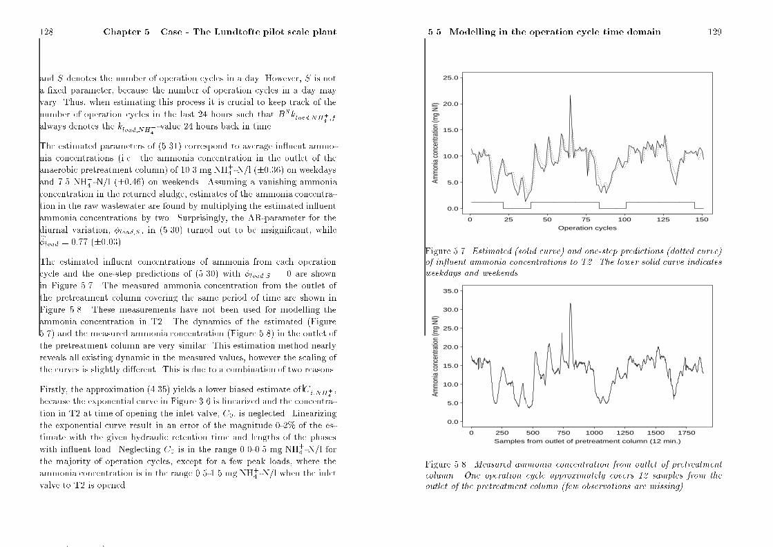
��� Chapter �� Case The Lundtofte pilot scale plant
and S denotes the number of operation cycles in a day� However S is not
a �xed parameter because the number of operation cycles in a day may
vary� Thus when estimating this process it is crucial to keep track of the
number of operation cycles in the last �� hours such that BSkload�NH��
�f
always denotes the kload�NH��
�value �� hours back in time�
The estimated parameters of ������ correspond to average in�uent ammo�
nia concentrations �i�e� the ammonia concentration in the outlet of the
anaerobic pretreatment column� of ��� mg NH �N�l � ���� on weekdays
and ��� NH �N�l � ���� on weekends� Assuming a vanishing ammonia
concentration in the returned sludge estimates of the ammonia concentra�
tion in the raw wastewater are found by multiplying the estimated in�uent
ammonia concentrations by two� Surprisingly the AR�parameter for the
diurnal variation �load�S in ����� turned out to be insigni�cant whileb�load ��� � ����
The estimated in�uent concentrations of ammonia from each operation
cycle and the one�step predictions of ����� with �load�S are shown
in Figure ���� The measured ammonia concentration from the outlet of
the pretreatment column covering the same period of time are shown in
Figure ���� These measurements have not been used for modelling the
ammonia concentration in T�� The dynamics of the estimated �Figure
���� and the measured ammonia concentration �Figure ���� in the outlet of
the pretreatment column are very similar� This estimation method nearly
reveals all existing dynamic in the measured values however the scaling of
the curves is slightly di�erent� This is due to a combination of two reasons�
Firstly the approximation ������ yields a lower biased estimate of Ci�NH��
because the exponential curve in Figure ��� is linearized and the concentra�
tion in T� at time of opening the inlet valve C is neglected� Linearizing
the exponential curve result in an error of the magnitude ��" of the es�
timate with the given hydraulic retention time and lengths of the phases
with in�uent load� Neglecting C is in the range ���� mg NH
�N�l for
the majority of operation cycles except for a few peak loads where the
ammonia concentration is in the range ������ mg NH �N�l when the inlet
valve to T� is opened�
��� Modelling in the operation cycle time domain ���
0 25 50 75 100 125 150
0.0
5.0
10.0
15.0
20.0
25.0
Operation cycles
Amm
onia
conc
entra
tion
(mg
N/l)
Figure ���� Estimated �solid curve� and onestep predictions �dotted curve�
of in�uent ammonia concentrations to T�� The lower solid curve indicates
weekdays and weekends�
0 250 500 750 1000 1250 1500 1750
0.0
5.0
10.0
15.0
20.0
25.0
30.0
35.0
Samples from outlet of pretreatment column (12 min.)Am
mon
ia co
ncen
tratio
n (m
g N/
l)
Figure ���� Measured ammonia concentration from outlet of pretreatment
column� One operation cycle approximately covers �� samples from the
outlet of the pretreatment column �few observations are missing��
� �

�� Chapter �� Case The Lundtofte pilot scale plant
Secondly in the models of the sampling time domain it is assumed that
approximately ��" of the increase in ammonia concentration during the
anoxic phase with in�uent load is produced by the hydrolysis and growth
of biomass� However the assumption of a constant positive net hydrolysis
rate could very well be wrong� There are strong reasons to believe that
the net hydrolysis process rate is actually zero or below zero in the anoxic
periods with in�uent load i�e� the ammonia uptake of the biomass is equal
to or above the production of ammonia by hydrolysis� If the additional
amount of ammonia required due to the higher denitri�cation in anoxic pe�
riods with in�uent load is taken into account the estimates of the ammonia
concentration in the outlet of the pretreatment column would be approx�
imately �" higher� Furthermore the storage of ammonia in the biomass
may be signi�cantly larger in periods with in�uent load�
The curves in Figure ��� reveals an important phenomenon for the mod�
elling of the in�uent load rate � rainy weather� Rainfall events give a high
�ow rate to the Lundtofte municipality plant while the �ow rate to the pi�
lot scale plant remains constant� On the other hand rainfall events result in
a low ammonia concentration of the raw wastewater which is loaded to the
pilot plant� Unfortunately information on the �ow rate to the Lundtofte
municipality plant for the analyzed period has not been obtainable for the
given period in a reasonable form but the rainy weather periods are clearly
recognized on Figure ��� where the estimated inlet concentration drops be�
low � mg NH �N�l� However these rainfall events cannot be predicted due
to lack of information on the �ow rate to the municipality plant� The rainy
weather periods of the time series also interrupt the diurnal pattern of in�
�uent ammonia concentrations resulting in the parameter for the diurnal
variation �load�S being insigni�cant� Thus if �ow rates to the Lundtofte
municipality plant were to be incorporated into ����� the model of the
in�uent ammonia load rate would be improved and �load�S would most
likely become signi�cant� This would also improve the variance of the error
terms in the process equation �e�load�NH��
signi�cantly� For the present
model the standard deviation of eload�NH��
�f is found to correspond to ���
mg NH �N�l for the estimated in�uent concentration of ammonia�
��� Modelling in the operation cycle time domain ���
Parameter Unit Ammonia Nitrate
�nit � ��� � ��� ��� � ���b�nit�max�� mg N�l�h ��� � ���� ��� � ���bKNH��
mg NH �N�l ��� � ��� ��� � ���be�nit�� mg N�l�h ��� ���
Table ���� Parameter estimates from modelling the maximum nitri�cation
process rate on data set No���
����� Maximum nitrication rate
In the sample time domain estimators of knit�max�NH��
�f and knit�max�NO��
�f
based on data from one operation cycle were derived by using ������ and
������ with the half�saturation constant KNH��
estimated on all available
observation in the data set� Due to lack of information on explanatory
variables which could describe some of the variations of knit�max�NH��
�f and
knit�max�NO��
�f �e�g� temperature C�N�ratio composition of wastewater�
a �rst order autoregressive model is proposed�
��� �nitB��knit�max���f � �nit�max��� enit�max���f ������
where �nit�max�� is the mean maximum nitri�cation rate estimated sep�
arately for the time series of ammonia and nitrate concentrations and
enit�max���f is NID with zero mean and variance �e�nit��� In case infor�
mation on explanatory variables in�uencing knit�max���f becomes available
�nit�max�� may be modelled as a function of those ������� The estimates of
this process are given in Table ���� A likelihood ratio test has shown that
the mean of the estimates from the two time series �nit�max ���� mg
N�l�h and KNH��
�� mg NH �N�l are reasonable estimates for both�
The estimated maximum nitri�cation rates bknit�max���f for each operation
cycle on observations of ammonia and nitrate concentrations are shown
in Figure ��� and Figure ��� as solid curves respectively� Estimates of
� �

��� Chapter �� Case The Lundtofte pilot scale plant
0 25 50 75 100 125 150
7.0
8.0
9.0
10.0
11.0
12.0
13.0
Operation cycles
Max
imum
am
mon
ia re
mov
al ra
te (m
g N/
l/h)
Figure ���� Estimated �solid curve� and onestep predictions �dotted curve�
of the maximum nitri�cation rate based on observations of ammonia con
centrations�
knit�max���f based on less than four observations in the sample time domain
have been rejected since the estimators ������ and ������ would not yield
reliable estimates on three or less observations� These estimates are treated
as missing values in the operation cycle time series indicated by the gaps
in the solid curves� The estimates related to the two series correspond
reasonably with each other except for a possible slight drift in the scaling
of one of the two FIA�analyzers�
As indicated on Figure ��� the one�step predictions of ������ are used as
parameter values in the sample time domain for the subsequent operation
cycle� The one�step predictions are given as dotted curves on Figure ���
and Figure ���� Thus the dotted should to some extend re�ect the dy�
namic of the solid curves� However the simple structure of ������ and
the estimated values of �nit compared to the dynamics of the estimated
maximum nitri�cation rates on the �gures indicate that ������ is not ap�
propriate for long�term predictions of knit�max���f because the model in fact
does not contain any physical knowledge� This is easily incorporated into
��� Modelling in the operation cycle time domain ���
0 25 50 75 100 125 150
7.0
8.0
9.0
10.0
11.0
12.0
13.0
Operation cycles
Max
imum
nitr
ate
form
ation
rate
(mg
N/l/h
)
Figure ���� Estimated �solid curve� and onestep predictions �dotted curve�
of the maximum nitri�cation rate based on observations of nitrate concen
trations�
the model if information on explanatory variables in�uencing knit�max���f
is available as described previously� In this case the estimates of �nit and
the variances of the prediction error �e�nit�� will become smaller�
Assuming that the suspended solids concentration and the oxygen con�
centration in the aerobic periods are maintained constant the activity of
autotrophic biomass is assessed applying the approximations ������ and
������� Inspecting the �gures it is seen that the activity of the autotro�
phic biomass may change by ���" within a few days� This e�ect cannot
be accounted for solely by the removal of excess sludge and the change in
the fraction of nitri�ers� Also it appears that some of the rainfall events
identi�ed from Figure ��� causes the maximum nitri�cation rate to drop
subsequently and high�low loads of ammonia causes the maximum nitri�
�cation rate to increase�decrease respectively� The rainy weather periods
might lower the overall temperature in the activated sludge causing the
� �

��� Chapter �� Case The Lundtofte pilot scale plant
Parameter Unit Nitrate
�denit � ��� � ���b�denit�max mg NO�� �N�l�h ��� � ����bKNO�
�
mg NO�� �N�l �� � ���bKload mg NH
�N�l�h ��� � ���be�denit mg NO�� �N�l�h ���
Table ���� Parameter estimates from modelling the maximum denitri�ca
tion process rate on data set No���
activity of the bacteria to decrease while the in�uence of the in�uent am�
monia load on the maximum nitri�cation rate is investigated in Chapter
������� Maximum denitrication rate
In the sample time domain an estimator of kdenit�max�f based on data from
one operation cycle was obtained by using ������ with the half�saturation
constants KNO��
and Kload estimated on the entire time series of nitrate
concentrations� A �rst order autoregressive model for describing the vari�
ations of kdenit�max�f is proposed�
��� �denitB��kdenit�max�f � �denit�max� edenit�max�f ������
where �denit�max is the mean maximumdenitri�cation rate and edenit�max�f
is NID with zero mean and variance �e�denit� Due to lack of informa�
tion on external variables capable of explaining some of the variations in
kdenit�max�f the mean maximum denitri�cation rate �denit�max is mod�
elled as a constant parameter� The estimates of this process are given in
Table ����
��� Modelling in the operation cycle time domain ���
0 25 50 75 100 125 150
2.0
3.0
4.0
5.0
6.0
7.0
Operation cycles
Max
imum
nitr
ate
rem
oval
rate
(mg
N/l/h
)
Figure ����� Estimated �solid curve� and onestep predictions �dotted curve�
of the maximum denitri�cation rate�
The estimated maximum denitri�cation rates bkdenit�max�f for each opera�
tion cycle are shown in Figure ���� with the one�step predictions of �������
Estimates of kdenit�max�f based on less than four observations have been
rejected since the estimator ������ would not yield reliable estimates on
fewer than four observations� These estimates are treated as missing values
in the operation cycle time domain which is indicated by the gaps of the
solid curve in Figure �����
Incorporating explanatory variables in ������ will most likely improve the
model and thereby reduce the variance of the prediction error �e�denit�
The trends of the curve �the slow dynamic� could be described by some
explanatory variables�
Assuming that the suspended solids concentration is maintained constant
the activity of the heterotrophic biomass is assessed applying the approxi�
mation ������� Similar to the variations of the maximum nitri�cation rate
the maximum denitri�cation rate appears to be in�uenced by the rainfall
events and the load of ammonia� However due to the assumption of using
� �
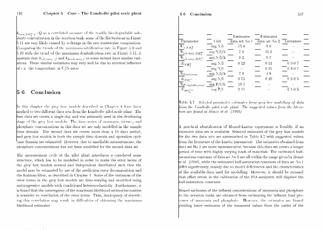
��� Chapter �� Case The Lundtofte pilot scale plant
kload�NH��
�f � Q as a correlated measure of the readily bio�degradable sub�
strate concentration in the aeration tank some of the �uctuations in Figure
���� are very likely caused by a change in the raw wastewater composition�
Comparing the trends of the maximum nitri�cation rate in Figure ��� and
��� with the trend of the maximum denitri�cation rate in Figure ���� it
appears that knit�max���f and kdenit�max�f to some extend have similar vari�
ations� These similar variations may very well be due to external in�uence
of e�g� the temperature or C�N�ratio�
�� Conclusion
In this chapter the grey box models described in Chapter � have been
applied to two di�erent data sets from the Lundtofte pilot scale plant� The
�rst data set covers a single day and was primarily used in the developing
stage of the grey box models� The time series of ammonia nitrate and
phosphate concentrations in this data set are only modelled in the sample
time domain� The second data set covers more than a �� days period
and grey box models in both the sample time domain and operation cycle
time domain are estimated� However due to unreliable measurements the
phosphate concentrations has not been modelled for the second data set�
The measurement cycle at the pilot plant introduces a correlated noise
structure which has to be modelled in order to make the error terms of
the grey box models normal and independent distributed such that the
model may be estimated by use of the prediction error decomposition and
the Kalman �lter as described in Chapter �� Some of the variances of the
error terms in the grey box models are time�varying and modelled using
autoregressive models with conditional heteroscedasticity� Furthermore it
is found that the convergence of the maximumlikelihood estimation routine
is sensitive to correlation of the error terms� Thus inadequacy of describ�
ing this correlation may result in di�culties of obtaining the maximum
likelihood estimates�
��� Conclusion ���
Estimates Estimates
Parameter Unit data set No�� data set No�� Literature
Ci�NH��
mg N�l ���� ��� �
knit�max�NH��
mg N�l�h ��� ��� �
knit�max�NO��
mg N�l�h ��� ��� �bKNH��
mg N�l ��� ��� �����
mg N�l � ��� �����
kdenit�max mg N�l�h �� ��� �bKNO��
mg N�l ��� �� �����
kP�uptake�max mg P�l�h ��� � �bKPO���
mg P�l ���� � �����
Table ���� Selected parameter estimates from grey box modelling of data
from the Lundtofte pilot scale plant� The suggested values from the litera
ture are found in Henze et al� �� ���
A practical identi�cation of Monod�kinetic expressions is feasible if an
extensive data set is available� Selected estimates of the grey box models
for the two data sets are summarized in Table ��� with suggested values
from the literature of the kinetic parameters� The estimates obtained from
data set No�� are more representative because this data set covers a longer
period of time with highly varying loads of materials� The estimated half�
saturation constants of data set No�� are all within the range given by Henze
et al� ����� while the estimated half�saturation constants of data set No��
di�er signi�cantly mainly due to model de�ciencies and the characteristics
of the available data used for modelling� However it should be stressed
that o�set errors in the calibration of the FIA�analyzers will displace the
half�saturation constants�
Biased estimates of the in�uent concentrations of ammonia and phosphate
to the aeration tanks are obtained from estimating the in�uent load pro�
cesses of ammonia and phosphate� However the estimates are biased
yielding lower estimates of the measured values from the outlet of the
� �

��� Chapter �� Case The Lundtofte pilot scale plant
pretreatment column� The estimated rate expression for the net in�uent
phosphate load consists of the rates of two distinct simultaneous processes
which cannot be separately identi�ed� These are the in�uent phosphate
load and the phosphate uptake during anoxic conditions� An estimate of
the phosphate uptake rate during anoxic conditions may be obtained by
combining the estimated net in�uent phosphate load with the measured
phosphate concentrations of the outlet of the pretreatment column� The
estimates of the ammonia load process is used as a correlated measure of
the readily bio�degradable substrate load for modelling the denitri�cation
process�
The activity of the autotrophic and heterotrophic biomass is assessed from
estimates of the nitri�cation and denitri�cation process in the operation
cycle time domain� However the models used to describe the variations
of this activity su�er from lack of information on the temperature C�N�
ratio wastewater composition and other explanatory variables having a
major in�uence on the biomass activity� The grey box models may be
improved if better data are available and some of the assumptions implied
in this chapter may be tested as well� Due to the constant throughput
of the pilot plant the in�uence of di�erent hydraulic loads has not been
investigated� This e�ect will be examined in the following chapter� Finally
it should be stressed that the interpretation of the estimates of the grey
box models should be done cautiously always keeping the standard error
of the estimates in mind�
Chapter �
Case � The Aalborg West
wastewater treatment
plant
This chapter deals with the estimation of grey box models on data from
the Aalborg West WWTP which is a well�monitored plant� The data from
the plant was made available in the last stage of this research project and
the models of this chapter represent a further re�nement of the models
estimated on data set No�� in Chapter �� Compared to the models of the
pilot scale plant the models of this chapter have two interesting aspects in
addition� Firstly the �ow rate to the plant is time�varying and secondly
the Aalborg West WWTP is a full�scale plant which in particular has an
impact on the hydraulic processes due to the large volume holding of the
aeration tanks� In addition the measurement system at the Aalborg West
WWTP does not introduce the same strong correlation in the measure�
ment noise sequence which makes it easier to model� The �rst section of
this chapter gives an introduction of the plant and the measurements avail�
able while the second and third section describes the estimated grey box
���
� �

�� Chapter �� Case The Aalborg West WWTP
models in the sample time domain and the operation cycle time domain
respectively� Some of the results of this chapter are also documented in
Carstensen et al� ������� It should be emphasized that the models pre�
sented in this chapter are derived by statistical methods from the class of
grey box models in Chapter � giving the best �t of data�
�� Introduction
The Aalborg West WWTP serves the Danish city of Aalborg with approx�
imately �� inhabitants� Figure ��� shows an aerial photograph of the
plant which was inaugurated in ����� It is designed for ��� PE �Person
Equivalent� with the purpose of treating the wastewater from the western
and central part of the city which formerly was discharged untreated to the
recipient a sound with brackish water� In the catchment area of the plant
a brewery abattoirs dairies and �sh processing industries produce some
high strength wastewater comprising at least two thirds of the organic load
to the plant� The design loads of the plant are given in Table ��� and Ein�
feldt ������ describes the implementation of biological nutrient removal on
the plant� The e�uent standards for the plant are �� mg BOD�l � mg to�
tal N�l �six months of summer� � mg total N�l �six months of winter� and
��� mg total P�l� The plant has an excellent performance and compliance
with the e�uent standard have been obtained from start of operation�
The wastewater handling facility of the plant consists of an inlet pumping
station � primary clari�ers an intermediate pumping station � anaerobic
pretreatment tanks �each subdivided into � separate anaerobic tanks in
series� � oxidation ditches and �� secondary clari�ers which is schemat�
ically shown in Figure ���� The WWTP is operated according to the
BIO�DENIPHO process� However a major part of the phosphate in the
wastewater is chemically precipitated by adding ferrosulphate�
The six oxidation ditches are operated in three parallel lines of two al�
ternating aeration tanks� Two of the oxidation ditches �denoted LT� and
��� Introduction ���
Figure ���� Aerial view of the Aalborg West WWTP� The aeration tanks
are located in the far end of the plant�
LT�� have been equipped with sensors for monitoring of ammonia and ni�
trate concentrations �both tanks� phosphate concentrations �only LT��
oxygen concentrations �two sensors in each tank� and suspended solids
concentrations �only LT��� The sampling points for some of the on�line
measurements are sketched in Figure ��� where the aeration tanks are
numbered from LT� to LT� starting from the bottom of the �gure� The
�ow rate to the biological part of the plant is also monitored� Furthermore
settings of the inlet and outlet weirs of the aeration tanks and the oxygen
supply rate �OSR� are registered� The oxygen supply rate is found from
the number of aeration rotors that has been switched on in the given aer�
ation tank for the last �ve minutes� Table ��� summarizes the monitored
� �

��� Chapter �� Case The Aalborg West WWTP
Flow Average Maximum
dry weather ��� m��day � m��day
�� m��h
rainy weather to plant �� m��h
to biology �� m��h
Pollution
BOD ��� kg�day ��� kg�day
SS ��� kg�day �� kg�day
Total�N ��� kg�day �� kg�day
Total�P �� kg�day �� kg�day
Table ���� Design loads for the Aalborg West WWTP� Data from Einfeldt
�� ���
2
3
1
4
1
2 3
1
Suspended Solids
Turbidity
Sludge blanket
Ammonia and Nitrate
5 Phosphate
Ret urn Sludge
Primary Clarif iers
An-aerobic Tanks
Secondary Clarif iers
Raw Wast ewat er
Secondary Clarif iers
Plant Ef f luent
Aerat ions t anks
LT6
LT5
LT4
LT3
LT2
LT1
4
4
5
On-line Measurements :
Figure ���� Schematic diagram of the wastewater treatment facility at the
Aalborg West WWTP�
��� Introduction ���
Variable Unit
Weir �inlet LT�� Wi�LT��t �� �closed�open�
Weir �inlet LT�� Wi�LT��t �� �closed�open�
Weir �outlet LT�� Wo�LT��t �� �closed�open�
Weir �outlet LT�� Wo�LT��t �� �closed�open�
Oxygen Supply Rate LT� OSRLT��t g O��h�m�
Oxygen Supply Rate LT� OSRLT��t g O��h�m�
Oxygen concentration LT� sensor � SO� �LT����t mg O��l
Oxygen concentration LT� sensor � SO� �LT����t mg O��l
Oxygen concentration LT� sensor � SO� �LT����t mg O��l
Oxygen concentration LT� sensor � SO� �LT����t mg O��l
Ammonia concentration LT� SNH�LT��t mg NH��N�l
Ammonia concentration LT� SNH�LT��t mg NH��N�l
Nitrate concentration LT� SNO��LT��t mg NO��N�l
Nitrate concentration LT� SNO��LT��t mg NO��N�l
Phosphate concentration LT� SPO�LT��t mg PO��N�l
SS concentration LT� XSS�LT��t g�l
Flow biological part of plant Qbio�t m��h
Table ���� Summary of available measurements and registered controlling
signals�
variables which have been used for modelling in this chapter with the ex�
ception that grey box models of the phosphate concentrations have not
been estimated on data from the Aalborg West WWTP because the time
series of phosphate concentrations do not re�ect much biological activity
due to chemical precipitation� The measurements of ammonia and nitrate
are the dependent variables to be modelled using past information from all
the variables listed in Table ����
The plant has been equipped with a SCADA system �Supervision Control
And Data Acquisition� called STAR �Superior Tuning And Reporting�
system see Nielsen Lynggaard�Jensen ������� where the measurements
of Table ��� are used as input for control of setpoints in the SCADA system�
� �

��� Chapter �� Case The Aalborg West WWTP
The controlling system is based on a set of rules combined with criteria func�
tions from empirical and mathematical expressions� The sensors used for
monitoring of nutrient salt concentrations have been chosen according to
an investigation in Thomsen Nielsen ������ such that su�cient stability
and low maintenance cost of the sensors are ensured�
From October ��th to November ��th ���� a data set of ��� observations
without large interrupts in the sampling was obtained� The time between
samples is four minutes and a few outliers and measurements taken during
calibration of the sensors has been removed from the data set and replaced
with missing values which are accordingly handled by the Kalman �lter�
The time of an average operation cycle is approximately � hours but it
may vary within the range from ��� to ��� hours due to the operation
strategies in the STAR�system� The total number of operation cycles in
the data set is ���� Hence there are su�cient observations for modelling
in the operation cycle time domain�
Some of the explanatory variables in Table ��� have large �uctuations due
to measurement noise� Thus in order to make use of these variables in
the grey box models a �ltering is required �e�g� a low�pass �ltering�� A
weighted moving average �lter with the �lter weights given below is found
adequate for these variables�
SO��LT��t ��SO��LT����t � �SO� �LT����t� �SO� �LT����t��
��SO� �LT����t��� SO� �LT����t��� SO� �LT����t������ �����
SO��LT��t ��SO��LT����t � �SO� �LT����t� �SO� �LT����t��
��SO� �LT����t��� SO� �LT����t��� SO� �LT����t������ �����
OSRLT��t �OSRLT��t � OSRLT��t��� OSRLT��t����� �����
OSRLT��t �OSRLT��t � OSRLT��t��� OSRLT��t����� �����
XSS�t �XSS�LT��t �XSS�LT��t�� �XSS�LT��t����� �����
Qbio�t �Qbio�t � Qbio�t��� Qbio�t����� �����
��� Modelling in the sample time domain ���
Alternatively the �lter weights could be designed from a frequency anal�
ysis of the esplanatory variables but applying such �lters in the grey box
models have very little e�ect on the description of data� The suspended
solids concentration in LT� is also assumed to be representative for the
suspended solids concentration in LT�� In order to determine which biolo�
gical processes are active at a given time the measurements of the oxygen
concentrations are used to divide the time series into aerobic and anoxic
periods using a hysteresis setting� Examination of data has shown that a
reasonable hysteresis setting is to change from aerobic to anoxic conditions
when the oxygen concentration drops below �� mg O��l and to change
from anoxic to aerobic conditions when the oxygen concentration exceeds
�� mg O��l� Employing the low�pass �ltered oxygen concentration with
the hysteresis setting distinct periods of aerobic and anoxic conditions are
determined �i�e� only one anoxic and one aerobic period in one operation
cycle�� Anaerobic periods rarely occur in the aeration tanks and for the
modelling of ammonia and nitrate concentrations anaerobic conditions have
little interest�
�� Modelling in the sample time domain
For modelling the time series of ammonia and nitrate concentrations at the
Aalborg West WWTP four hydraulic and biochemical processes may be
identi�ed�
� In�uent ammonia load�
� Transport of nutrients
� The nitri�cation process
� The denitri�cation process
The hydrolysis and growth of biomass process cannot be identi�ed for the
given data set because the anoxic periods of the time series without in�u�
ent load to the aeration tanks �i�e� the periods where the hydrolysis and
� �

��� Chapter �� Case The Aalborg West WWTP
growth of biomass normally is the most signi�cant process for the ammonia
concentration� are few and short� Secondly attempts to estimate the rate
of hydrolysis and growth of biomass process in these periods failed due to
statistical insigni�cance�
The rate expressions for the signi�cant processes above are more exten�
sive compared to the rate expressions for the processes at the Lundtofte
pilot scale plant given in Chapter �� This is due to the monitoring of
the suspended solids concentration and the use of di�erent oxygen set�
points during the aerobic phases� With this information available grey
box models almost identical to those presented in Section ��� are formu�
lated� Furthermore the monitoring of ammonia and nitrate concentrations
in both LT� and LT� give rise to double estimates of the same processes�
Hence the validity of the grey box models is investigated by comparing the
estimates from the two tanks�
One major di�erence between the models of the previous chapter and the
models of this chapter is the variable �ow rate to the biological part of
Aalborg West WWTP� The diurnal �ow rate of a typical dry weather day
is depicted in Figure ��� �see page �� while the total daily �ow for the
�� days period is depicted in Figure ���� The highly varying �ow rate to
the plant give rise to strong variations in the dynamics of the wastewater
processes especially during peak hydraulic loads caused by rainy weather�
However information obtained from measurements of the �ow rate to the
plant is used to detect the occurrences of rainfall events and the conse�
quently low in�uent ammonia concentration� Recalling the discussion in
Section ����� the lack of information on rainfall events at the pilot scale
plant is an evident de�ciency of the model for the in�uent load rate of
ammonia in the operation cycle time domain ������
The observation equation for the time series of ammonia and nitrate are
as usual given by
yt mt � �t �����
��� Modelling in the sample time domain ���
where mt is the true concentration of ammonia or nitrate and �t is Normal
and Independent Distributed �NID� with zero mean and variance given by
an ARCH�structure �Tong ������ i�e�
���t ��� � ����
t�� �����
where �t�� in ����� is replaced by the prediction error vt�� for practical
applications and �� is a parameter�
The process equation for each of the four time series of ammoniaand nitrate
concentrations is found to be adequately modelled using
��� �B��!mt � �t� �Tut � et �����
where et is NID with zero mean and a variance which is found to be con�
ditional on the previous concentration level i�e�
�e�t �e� � �em�
t�� �����
where �e� and �e are parameters� Hence the process equation ����� is
better at modelling low level concentrations than high level concentrations�
Two explanations for this phenomenon are given� Firstly the steps of
the concentration gradient !mt are larger for high level concentrations
resulting in larger error terms et� Secondly switching from aerobic to
anoxic conditions and reverse introduces some noise into the processes
which is partly modelled as transient phenomena� The switching from
aerobic to anoxic conditions and reverse cannot be clearly de�ned by simply
choosing an oxygen concentration threshold dividing aerobic and anoxic
periods� Therefore the ammonia and nitrate concentrations on top of
the time series curves are more unpredictable� The mean of the posterior
distribution bmt��jt�� is used as the optimal estimator of mt�� in ������
The AR�parameter estimates b� are in the range ������� � ��� which is
somewhat larger than those estimated on data set No�� from the pilot plant�
� �

��� Chapter �� Case The Aalborg West WWTP
This implies that the mean process rate �t does not give as persistent an
estimate of the concentration gradient for the models of this chapter�
����� Inuent ammonia load in dry weather
The ammonia load to AalborgWest WWTP is modelled according to ������
during dry weather periods with kload�NH��
being a time�varying parameter
of the operation cycle time domain �see following section� i�e�
rload�NH��
�t �
kload�NH��
�f �Q�
bio�t�� inlet weir open
inlet weir closed
������
where Q�
bio�t�� is the �ltered �ow rate of wastewater and returned sludge
entering the BIO�DENIPHO line consisting of LT� and LT�� The �ow rate
to the biological part of the plant Qbio�t is equally mixed with returned
sludge and then divided into three parallel lines of alternating aeration
tanks� Thus
Q�
bio�t�� �Qbio�t��
�
������
The rate of the returned sludge may vary slightly below the in�uent �ow
rate but this does not a�ect the applicability of the model� Using the data
from one operation cycle an estimate of kload�NH��
�f is obtained from ������
which can be used for updating the models of the in�uent ammonia load
rate in the operation cycle time domain� An estimate of the in�uent ammo�
nia concentration to the aeration tanks is obtained from the approximation
������ but the estimator will be biased as discussed in Section ������ The
ammonia load rate kload�NH��
�f �Q�
bio�t�� is also used as a correlated mea�
sure for the load of readily bio�degradable substrate which is employed for
modelling of the denitri�cation process�
��� Modelling in the sample time domain ���
����� Inuent ammonia load with rainy weather peri�
ods
A rainfall event in the catchment area is typically characterized by a large
volume of low loaded wastewater entering the WWTP due to the mixing
of wastewater produced by households and industries and rainwater� How�
ever when modelling a rainfall event some allowances for the large bu�er
of wastewater in the sewerage should be made� In Figure ��� an ideal�
ized picture of a typical rainfall event is sketched� This illustration is used
to derive a simpli�ed model for the ammonia load rate in rainy weather
periods�
When rain starts falling in the catchment area the �ow of rainwater and
produced wastewater into the sewerage increases momentarily� The ammo�
nia concentration of the mixed rainwater and produced wastewater conse�
quently drops to a lower concentration which in this simpli�ed model is
assumed to be constant� When the rainfall event subsequently stops only
wastewater from households and industries is �ushed into the sewer� Conse�
quently the �ow rate and ammonia concentration of the wastewater return
to the dry weather levels� At the WWTP the �ow rate increases shortly
after the rain has started falling� However due to a large bu�er of highly
loaded wastewater in the sewerage the in�uent ammonia concentration of
the raw wastewater to the plant slowly decreases towards the low ammo�
nia concentration of produced wastewater mixed with rainwater running
into the sewer� Similarly when the rain stops falling the �ow rate to the
plant decreases rather fast after a short period of time while the in�uent
ammonia concentration to the plant slowly increases towards the ammonia
concentration level of produced wastewater due to the large bu�er of low
loaded wastewater in the sewerage�
The rainy weather periods are detected from the measurements of the �ow
rate to the biological part of the plant despite the fact that during rain�
falls a signi�cant part of the raw wastewater is bypassed i�e� all the raw
wastewater is mechanically processed and a fraction of this wastewater is
led to the e�uent of the plant without biological treatment� The start of a
� �

�� Chapter �� Case The Aalborg West WWTP
����������������������������������������������������������������������������������������������������������������������������������������������
Flow
������������������������������������������������������������������������������������������������������������������������������������������������
tstoptstart
To WWTP�
To sewerage�
Ammonia conc�
Flow
Ammonia conc�
Figure ���� Illustration of the dynamics in the sewerage during a rainy
weather period� The two points in time� tstart and tstop� show the length of
the rainy weather period determined by the measured �ow rate to the plant�
rainfall event is de�ned as Qbio�t exceeding � m��h and it is considered
to be �nished when Qbio�t has been below �� m��h for two hours� The
starting and stopping time of a rainfall event are denoted tstart and tstop
as indicated on Figure ��� and the length of the rainy weather period is
given by tstop � tstart�
The large bu�er volume of the sewerage primary clari�ers and anaerobic
pretreatment tanks that the wastewater has to pass before entering the
aeration tanks can neither be considered as one big ideally mixed tank nor
as one large pipe without mixing� In particular partially mixing occur in
��� Modelling in the sample time domain ���
the sewerage due to varying hydraulic retention times of the di�erent sub�
sewerages and the geographical movement of the precipitation� In order
to describe the partial mixing of produced wastewater with rainwater in
the large bu�er volume of the sewerage primary clari�ers and anaerobic
pretreatment tanks a simple model of N ideally mixed tanks with identical
volume holdings in series is found adequate�
The response of a step�function load on N identical ideally mixed tanks in
series is obtained by successively applying ����� with the response of the
n�th tank being the input to the n � ��th tank �n N �� The response is
most conveniently found by applying the Laplace transformation�
Ct Ci��� e� tTh �
tThe� tTh � � � ��
tN��
�N � ��)TN��
h
e� tTh � ������
where Ci is the in�uent concentration to the �rst tank and Th is the
hydraulic retention time of the individual ideally mixed tanks� The concen�
tration in all N tanks at the starting time of the step�function is assumed
to be constant and Ct is the deviation from this steady state level�
Thus in order to incorporate the e�ects of rainy weather on the in�uent
ammonia load rate ������ needs to be modi�ed�
rload�NH��
�t �
k�
load�NH��
�f�t�Q
�bio�t�� inlet weir open
inlet weir close
������
wherek�
load�NH��
�f�t kload�NH�
�
�f � �kload�NH��
�f � krain� � �N �t � tstop�
� �krain � kload�NH��
�f � � �N �t� tstart� ������
and
� �
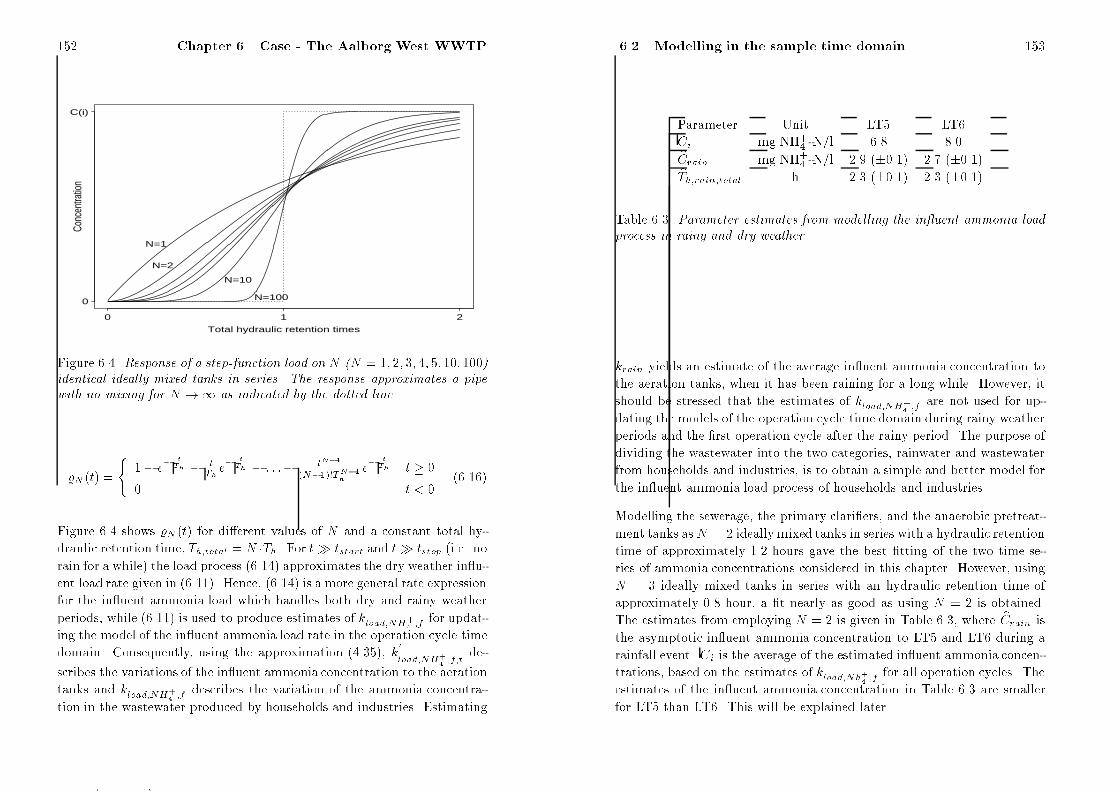
��� Chapter �� Case The Aalborg West WWTP
0 1 2
0
C(i)
Total hydraulic retention times
Conc
entra
tion
N=1
N=2
N=10
N=100
Figure ���� Response of a stepfunction load on N �N �� �� �� �� ������
identical ideally mixed tanks in series� The response approximates a pipe
with no mixing for N �� as indicated by the dotted line�
�N �t� �
�� e� tTh � t
The� tTh � � � �� tN��
�N����TN��
h
e� tTh t �
t
������
Figure ��� shows �N �t� for di�erent values of N and a constant total hy�
draulic retention time Th�total N �Th� For t� tstart and t� tstop �i�e� no
rain for a while� the load process ������ approximates the dry weather in�u�
ent load rate given in ������� Hence ������ is a more general rate expression
for the in�uent ammonia load which handles both dry and rainy weather
periods while ������ is used to produce estimates of kload�NH��
�f for updat�
ing the model of the in�uent ammonia load rate in the operation cycle time
domain� Consequently using the approximation ������ k�
load�NH��
�f�tde�
scribes the variations of the in�uent ammonia concentration to the aeration
tanks and kload�NH��
�f describes the variation of the ammonia concentra�
tion in the wastewater produced by households and industries� Estimating
��� Modelling in the sample time domain ���
Parameter Unit LT� LT�
Ci mg NH �N�l ��� ��bCrain mg NH
�N�l ��� � ��� ��� � ���bTh�rain�total h ��� � ��� ��� � ���
Table ���� Parameter estimates from modelling the in�uent ammonia load
process in rainy and dry weather�
krain yields an estimate of the average in�uent ammonia concentration to
the aeration tanks when it has been raining for a long while� However it
should be stressed that the estimates of kload�NH��
�f are not used for up�
dating the models of the operation cycle time domain during rainy weather
periods and the �rst operation cycle after the rainy period� The purpose of
dividing the wastewater into the two categories rainwater and wastewater
from households and industries is to obtain a simple and better model for
the in�uent ammonia load process of households and industries�
Modelling the sewerage the primary clari�ers and the anaerobic pretreat�
ment tanks as N � ideallymixed tanks in series with a hydraulic retention
time of approximately ��� hours gave the best �tting of the two time se�
ries of ammonia concentrations considered in this chapter� However using
N � ideally mixed tanks in series with an hydraulic retention time of
approximately �� hour a �t nearly as good as using N � is obtained�
The estimates from employing N � is given in Table ��� where bCrain is
the asymptotic in�uent ammonia concentration to LT� and LT� during a
rainfall event� Ci is the average of the estimated in�uent ammonia concen�
trations based on the estimates of kload�Nh��
�f for all operation cycles� The
estimates of the in�uent ammonia concentration in Table ��� are smaller
for LT� than LT�� This will be explained later�
� �

��� Chapter �� Case The Aalborg West WWTP
����� Nutrient transport of the aeration tanks
Incorporating the mass balance of nutrients is important but not crucial for
obtaining interpretable estimates of the remaining wastewater processes�
Fortunately both aeration tanks at Aalborg West WWTP are equipped
with on�line sensors of ammonia and nitrate concentrations� Thus for the
transport of ammonia
rtransport�NH��
�t �����
ktransport�NH��
�SINH��
�t��� SNH�
�
�t��� �Qt��
outlet weir open
otherwise
������
and for the transport of nitrate
rtransport�NO��
�t ���������
ktransport�NO��
�SINO��
�t��� SNO�
�
�t��� �Qt��
inlet weir closed and outlet weir open
�ktransport�NO��
� SNO��
�t�� �Qt�� inlet weir open
otherwise
������
where SINH��
�t��and SINO��
�t��are the ammonia and nitrate concentrations
of the alternating tank� SINH��
�t��and SINO��
�t��are replaced by the mea�
surements of the ammonia and nitrate concentrations in the alternating
tank while SNH��
�t�� and SNO��
�t�� are replaced by the optimal estimates
of the true ammonia and nitrate concentration bmt��jt��� The estimated
parameters of the model are given in Table ����
The estimates of k��transport�� are larger than the actual physical holding
volumes of the aeration tanks ��� m��� This is mainly due to lack of
information on the hydraulic e�ects when switching �ow patterns i�e� the
wastewater levels in the two alternating tanks are di�erent and switching
the in�uent and e�uent �ow between the two tanks will gradually result
��� Modelling in the sample time domain ���
ktransport�� Unit LT� LT�
Ammonia ��m�� ��� � ��� ���� � ���
Nitrate ��m�� ���� � ��� ���� � ���
k��transport�� Unit LT� LT�
Ammonia m� ��� ��� ��� � �� �� �� �
Nitrate m� �� ��� ��� � �� ��� � �
Table ���� Parameter estimates from modelling the nutrient transport of
the aeration tanks�
in a change of �ow between the two tanks� This will make the estimates of
ktransport�� smaller�
����� The nitrication process
The monitoring of ammonia and nitrate concentrations in both LT� and
LT� permits the identi�cation of the nitri�cation process from four dif�
ferent time series� Thus if the estimates from the four time series show
consistency this will validate the general model structure� In the considered
period of time the plant has been operated with di�erent oxygen setpoints
where the employment of two oxygen sensors in each tank combined with
the �ltering ����� and ����� has made the identi�cation of a Monod�kinetic
term for the dependency of the oxygen concentration possible� Further�
more due to the monitoring of the suspended solids concentration expres�
sions like ������ and ������ are identi�ed� However during high loads at
the Aalborg West WWTP the rotors must have been turned on for a while
before the oxygen concentration reaches its setpoint� This period of time is
considered anoxic because of the low oxygen concentration but ammonia
is in fact nitri�ed due to an excessive amount of oxygen being aerated into
the aeration tanks� Fortunately the oxygen supply rate is registered and it
is assumed that nitri�cation rate is proportional to OSRt�� in this period�
Thus for the time series of ammonia concentrations
� �

��� Chapter �� Case The Aalborg West WWTP
rnit�NH��
�t �������
�knit�max�NH��
�
SNH
��
�t��
SNH
��
�t��KNH
��
�
SO��t��
SO��t��KO�
�XSS�t��
aerobic conditions
�kOSR�NH��
�OSRt�� anoxic�anaerobic conditions
������
and for the time series of nitrate concentrations
rnit�NO��
�t �������
knit�max�NO��
�
SNH
��
�t��
SNH
��
�t��KNH
��
�
SO��t��
SO� �t��KO�
�XSS�t��
aerobic conditions
kOSR�NO��
�OSRt�� anoxic�anaerobic conditions
�����
where SO� �t�� XSS�t�� and OSRt�� are replaced with the �ltered values
given in ��������� for the practical identi�cation� The mean of the posterior
distribution for mt�� is used as the optimal estimator of the true ammo�
nia concentration in the aeration tanks i�e� SNH��
�t�� is replaced by the
Kalman update bmt��jt�� in ������ and ������ The results of estimating
the nitri�cation process on data from Aalborg West WWTP are given in
Table ����
Fortunately there is a consistency between the estimates of the nitri�ca�
tion process obtained from the four time series in Table ��� validating the
general grey box model structure for the nitri�cation process� Though
the estimates from the time series of ammonia concentrations in LT� di�er
slightly� The reason for this is explained in the subsequent section� Henze
et al� ����� suggest thatKNH��
should lie in the range �����mgNH �N�l
and KO�
should lie in the range ����� mg O��l� Thus all the estimated
half�saturation parameters values are in the suggested range except forbKNH��
estimated on measurements of the ammonia concentration in LT��
However due to the discrete time formulation of the Monod�kinetic ex�
pressions the grey box models will yield biased and larger estimates of the
half�saturation constants in continuous time as discussed in Section ������
��� Modelling in the sample time domain ���
Parameter Unit LT� LT�
Ammonia knit�max�NH��
mg N�h�g SS ��� ����bKNH��
mg N�l ��� � ��� ��� � ���bKO�
mg O��l ��� � ��� ��� � ���bkOSR�NH��
mg N�g O� ���� � ��� ���� � ���
Nitrate knit�max�NO��
mg N�h�g SS ��� ����bKNH��
mg N�l �� � ��� ��� � ���bKO�
mg O��l ��� � ��� ��� � ���bkOSR�NO��
mg N�g O� ���� � ���� ���� � ����
Table ���� Parameter estimates from modelling the nitri�cation process on
data from Aalborg West WWTP�
The estimates of knit�max�NO��
�f are less biased estimates of the maximum
nitri�cation rate than knit�max�NH��
�f because the hydrolysis and growth of
biomass process is not incorporated in the grey box models of the Aalborg
West WWTP� Hence knit�max�NH��
�f is an estimator of the net maximum
nitri�cation rate which includes the simultaneous removal of ammonia by
nitri�cation and growth of biomass and production of ammonia by hy�
drolysis� This is also re�ected in the lower estimates of knit�max�NH��
�f and
kOSR�NH��
in Table ���� In fact in the anoxic periods with the rotors turned
on twice as much nitrate is produced as ammonia removed� The e�ect of
aerating during anoxic conditions on the denitri�cation rate is neglected
but it is a topic for future research� Comparing the stoichiometric coe��
cient of ����� with the estimates of kOSR�� it is seen that ����" of the
oxygen supplied by the rotors in the anoxic period is used for nitri�cation
while the rest of the oxygen supplied is used for heterotrophic respiration
and in particular raising the overall oxygen concentration in the aeration
tank to the setpoint value� Given the values of bKNH��
and bKO�
estimated
on the entire data set estimates of knit�max���f are obtained from the data
of operation cycle f �
� �

��� Chapter �� Case The Aalborg West WWTP
����� The denitrication process
Assuming that the load rate of ammonia is highly correlated with the aver�
age concentration of readily bio�degradable substrate in the aeration tanks
during the anoxic phase with in�uent load the following expression is iden�
ti�ed�
rdenit�t ����������� anoxic conditions and no in�uent load
�kdenit�max�f
SNO�
�
�t��
SNO�
�
�t��KNO�
�
�
kload�NH
��
�f���Qt��
kload�NH
��
�f���Qt��KloadXSS�t��
anoxic conditions and in�uent load
aerobic�anaerobic conditions
������
where Qt�� andXSS�t�� are replaced with the �ltered values given in ������
and ����� for the practical identi�cation of ������� The mean of the posterior
distribution for mt�� is used as the optimal estimator of the true nitrate
concentration in the aeration tank i�e� SNO��
�t�� is replaced by the Kalman
update bmt��jt�� in ������� The estimated ammonia load parameter of
the previous operation cycle in both dry and rainy weather bk�load�NH��
�f��
given by ������ is used in the second Monod�kinetic term in ������� It
should be stressed that the rate of the denitri�cation process during anoxic
conditions without in�uent load is found to be insigni�cant mainly due to
lack of readily bio�degradable substrate in LT� and LT� after the aerobic
phase� This result corresponds to the similarly very low and insigni�cant
hydrolysis and growth of biomass process rate� The results of estimating
the denitri�cation process on data from Aalborg West WWTP are given
in Table ����
Similar to the estimates of the nitri�cation process the estimates in Ta�
ble ��� are consistent for the two time series� Though the estimates of
KNO��
are somewhat higher than the suggested values of the literature
�Henze et al� ����� suggest KNO��
lies in the range ����� mg NO�� �N�l��
This may be due to de�ciencies in� �� the assumption of high correlation
��� Modelling in the sample time domain ���
Parameter Unit LT� LT�
kdenit�max mg N�h�g SS ��� ����bKNO��
mg N�l ��� � ��� ��� � ����bKload mg N�l�h ���� � ��� ���� � ����
Table ���� Parameter estimates from modelling the denitri�cation process
on data from Aalborg West WWTP�
between the ammonia load rate and the load of readily bio�degradable ma�
terial and �� the assumption of a constant in�uent load rate of organic
materials resulting in a constant concentration of readily bio�degradable
substrate� However in the absence of sensors for monitoring the readily
bio�degradable substrate on�line the denitri�cation process is more ade�
quately described in ������ than leaving the second Monod�kinetic term
out� Using the design loads in Table ��� for the Aalborg West WWTP
and applying three assumptions the estimates of Kload are interpreted in
terms of BOD� First assumption is that the in�uent concentrations of am�
monia and BOD are left unaltered by passage of the pretreatment tanks�
Secondly it is assumed that �" of the total nitrogen to the plant is in
the form of ammonia using Table ��� for moderately loaded wastewater�
Thirdly BOD in returned sludge is not used for denitri�cation� Based
on these assumptions the estimates of Kload corresponds to bKS ��� mg
BOD�l � ��� for LT� and bKS ��� mg BOD�l � ��� for LT�� Finally
using the COD�BOD�ratio for moderately loaded wastewater in Table ���
the estimates of KS are found to lie in the range ��� mg COD�l as
suggested by Henze et al� ������
Given the estimates of KNO��
and Kload based on the entire time series
of measurements of nitrate concentrations estimates of kdenit�max�f are
obtained from the observations of operation cycle f � These estimates are
used for updating the model of the maximum denitri�cation rate in the
operation cycle time domain�
� �
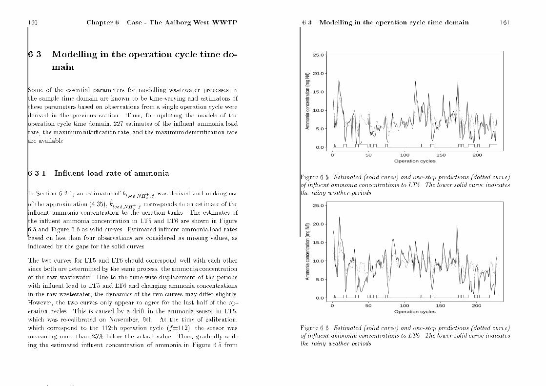
�� Chapter �� Case The Aalborg West WWTP
�� Modelling in the operation cycle time do�
main
Some of the essential parameters for modelling wastewater processes in
the sample time domain are known to be time�varying and estimators of
these parameters based on observations from a single operation cycle were
derived in the previous section� Thus for updating the models of the
operation cycle time domain ��� estimates of the in�uent ammonia load
rate the maximumnitri�cation rate and the maximumdenitri�cation rate
are available�
����� Inuent load rate of ammonia
In Section ����� an estimator of kload�NH��
�f was derived and making use
of the approximation ������ bkload�NH��
�f corresponds to an estimate of the
in�uent ammonia concentration to the aeration tanks� The estimates of
the in�uent ammonia concentration in LT� and LT� are shown in Figure
��� and Figure ��� as solid curves� Estimated in�uent ammonia load rates
based on less than four observations are considered as missing values as
indicated by the gaps for the solid curves�
The two curves for LT� and LT� should correspond well with each other
since both are determined by the same process the ammonia concentration
of the raw wastewater� Due to the time�wise displacement of the periods
with in�uent load to LT� and LT� and changing ammonia concentrations
in the raw wastewater the dynamics of the two curves may di�er slightly�
However the two curves only appear to agree for the last half of the op�
eration cycles� This is caused by a drift in the ammonia sensor in LT�
which was re�calibrated on November �th� At the time of calibration
which correspond to the ���th operation cycle �f ���� the sensor was
measuring more than ��" below the actual value� Thus gradually scal�
ing the estimated in�uent concentration of ammonia in Figure ��� from
��� Modelling in the operation cycle time domain ���
0 50 100 150 200
0.0
5.0
10.0
15.0
20.0
25.0
Operation cycles
Amm
onia
conc
entra
tion
(mg
N/l)
Figure ���� Estimated �solid curve� and onestep predictions �dotted curve�
of in�uent ammonia concentrations to LT�� The lower solid curve indicates
the rainy weather periods�
0 50 100 150 200
0.0
5.0
10.0
15.0
20.0
25.0
Operation cyclesAm
mon
ia co
ncen
tratio
n (m
g N/
l)
Figure ���� Estimated �solid curve� and onestep predictions �dotted curve�
of in�uent ammonia concentrations to LT�� The lower solid curve indicates
the rainy weather periods�
� �

��� Chapter �� Case The Aalborg West WWTP
f to ��� yields a dynamic similar to that of Figure ���� The mis�
calibration of the ammonia sensor in LT� also explains the low estimates of
the average in�uent ammonia concentration in Table ��� and the average
maximumnitri�cation rate in Table ��� when estimated on data from LT��
The ammonia concentration of the raw wastewater is approximately twice
the estimated in�uent ammonia concentration because the raw wastewater
is equally mixed with returned sludge with a vanishing ammonia concen�
tration� Though in the discussion of Section ����� it was found that the
estimator kload�NH��
�f yields lower biased estimates of the actual in�uent
ammonia load rate� Hence the ammonia concentration of the raw waste�
water is presumably more than twice the estimated curves of Figure ���
and ����
The in�uent load rate of ammonia to the WWTP arising from households
and industries show typical diurnal and weekly patterns due to human
behaviour� Thus formulating a model for kload�NH��
�f these basic human
activities are sought captured�
�� � �loadB��kload�NH��
�f � �load�NH��
�t� eload�NH��
�f ������
where eload�NH��
�f is NID with zero mean and variance �e�load�NH��
and
�load�NH��
�f describes the diurnal variation using a second�order Fourier
expansion and type�of�day e�ects
�load�NH��
�t �
�weekday�NH��
� �t if operation cycle f is on a weekday
�weekend�NH��
� �t if operation cycle f is on a weekend
������
and
�t � � �� cos��t
S
� � sin��t
S
� �� cos��t
S
� � sin��t
S
������
��� Modelling in the operation cycle time domain ���
where S �� is the number of samples in a day� The diurnal pro�le �t
is assumed to be identical on weekdays and weekends� The AR����process
in ������ describes the correlated deviations from the average mean load
of ammonia �load�NH��
�t from one operation cycle to another i�e� if the
ammonia load of the last operation cycle was lower than the mean load
of ammonia at the given time ������ it is likely that the ammonia load of
the present operation cycle will also be lower� The one�step predictions of
������ are shown as dotted curves in Figure ��� and Figure ��� for LT� and
LT� respectively�
In the rainy periods which are indicated by the lower curves on Figure
��� and ��� the model ������ is not updated with the estimated ammonia
load rates because ������ describes the ammonia load of households and
industries� Therefore during the rainfall events the one�step predictions of
kload�NH��
�f will approach �load�NH��
�t while the actual ammonia load rate
is modelled by ������ in the sample time domain� Besides the rainy weather
periods the one�step predictions of ������ corresponds to the estimated
in�uent ammonia load rate except for short term peak loads which are
di�cult to predict as they cannot be described as simple diurnal variations
and they have not been found correlated with other measurements at the
WWTP�
The estimates of kload�NH��
�f obtained from the data of one operation cycle
are encumbered with some uncertainty
bkload�NH��
�f kload�NH��
�f � �load�NH��
�f ������
where �load�Nh��
�f is NID with zero mean and variance �
�load�NH��
�
The process equation ������ and observation equation ������ for the in�uent
ammonia load rate process has a state space representation which can be
handled by applying the Kalman �lter� Hence the variances of the error
terms can be estimated by the maximumlikelihood approach if appropriate
weights for the prediction errors in the sample time domain relative to the
prediction errors in the operation cycle time domain are supplied in the
� �

��� Chapter �� Case The Aalborg West WWTP
calculation of the likelihood function� Alternatively if the variance of the
prediction error in the operation cycle time domain is assumed to be time�
invariant ����� estimates of �e�load�NH��
and ��load�NH��
are obtained by
estimating the constant Kalman gain Kload�NH��
and the variance of the
prediction error Rload�NH��
� This will be shown in the following� Due to
the simple form of ������ all the variables for the Kalman �lter are scalar�
From the sequence of prediction errors of the in�uent ammonia load process
vload�f f �� � � � � ��� an estimate of the variance of the predictions errors
is obtained bRload�NH��
� Thus with the estimated Kalman gain and ������
where c � is scalarbPload�NH�
�
bKload�NH��
� bRload�NH��
������
The estimates of the variances of the error terms in ������ and ������
are found applying the prediction equation of bPload�NH��
to ������ andbRload�NH��
to ������b�e�load�NH��
bPload�NH��
��� b��load� ������
and
b��load�NH��
bRload�NH��
� bPload�NH��
������
The estimates of the in�uent ammonia load process are given in Table ���
where the standard deviations of the error terms and the average mean
in�uent ammonia loads are listed using the equivalent in�uent ammonia
concentrations�
The estimates of �load in Table ��� are somewhat smaller than the estimates
obtained from data set No�� at the pilot plant due to the incorporation of
a rainy weather ammonia load model� The estimates of the mean in�uent
ammonia concentration and the standard deviations of the error terms in
��� Modelling in the operation cycle time domain ���
Parameter Unit LT� LT�b�weekday�NH��
mg N�l �� � ��� ��� � ���b�weekday�NH��
mg N�l ��� � ��� ��� � ���b�load � ��� � ��� �� � ���be�load mg N�l ��� ���b�load mg N�l ��� ���
Table ���� Parameter estimates from modelling the in�uent ammonia load
rate process in the operation cycle time domain�
the LT� column are too low due to the bad calibration of the ammonia
sensor in LT� as mentioned previously� The standard deviations of the
error terms are in general rather high showing that the model ������ will
predict the in�uent ammonia concentration within an interval of �� mg
NH �N�l with a probability of ��"� This is mainly due to bad model per�
formance of predicting peak in�uent ammonia concentration� The in Table
��� estimates could be improved by applying a robust estimation procedure
where the peak loads have a relative small weight in the calculation of the
likelihood function and the estimation of the variance of the prediction er�
ror Rload�NH��
� However a large number of the peak loads are caused by
dewatering of excess sludge as a part of the plant operation� Thus it is
preferable to incorporate knowledge on the times of the excess sludge de�
watering into the model if such information can be obtained� Disregarding
the peak loads in Figure ��� and ��� the standard deviations of eload�NH��
�f
graphically appears to be much lower�
����� Maximum nitrication rate
From the slopes of ammonia and nitrate curves during the aerobic phase of
the operation cycle estimates of knit�max���f are obtained given the values
of KNH��
and KO�
estimated on all available observations� These estimates
are naturally encumbered with some uncertainty
� �

��� Chapter �� Case The Aalborg West WWTP
0 50 100 150 200
0.0
0.5
1.0
1.5
2.0
Operation cycles
Max
imum
am
mon
ia re
mov
al ra
te (m
g NH
4-N/
h/g
SS)
Figure ���� Estimated �solid curve� and onestep predictions �dotted curve�
of maximum nitri�cation rates based on ammonia concentrations from aer
ation tank LT��
bknit�max���f knit�max���f � �nit�max���f ������
where �nit�max���f is NID with zero mean and variance ��nit�� and the in�
dexed period indicates that ������ is valid for the modellingof knit�max�NH��
�f
and knit�max�NO��
�f on data from both aeration tanks� Thus four sets of
estimates from this process are obtained� The estimated maximum nitri�
�cation rates from the four considered time series bknit�max���f for each
operation cycle are shown in Figure ������� by the solid curves� Estimates
of knit�max���f based on less than four observations in the sample time do�
main are rejected due to unreliable estimates�
The variations of the maximumnitri�cation rate are modelled using a �rst�
order AR�process
�� � �nitB��knit�max���f � �nit�max���f� enit�max���f �����
��� Modelling in the operation cycle time domain ���
0 50 100 150 200
0.0
0.5
1.0
1.5
2.0
Operation cycles
Max
imum
am
mon
ia re
mov
al ra
te (m
g NH
4-N/
h/g
SS)
Figure ���� Estimated �solid curve� and onestep predictions �dotted curve�
of maximum nitri�cation rates based on ammonia concentrations from aer
ation tank LT��
0 50 100 150 200
0.0
0.5
1.0
1.5
2.0
2.5
Operation cyclesM
axim
um n
itrat
e fo
rmat
ion ra
te (m
g NO
3-N/
h/g
SS)
Figure ���� Estimated �solid curve� and onestep predictions �dotted curve�
of maximum nitri�cation rates based on nitrate concentrations from aera
tion tank LT��
� �

��� Chapter �� Case The Aalborg West WWTP
0 50 100 150 200
0.0
0.5
1.0
1.5
2.0
2.5
Operation cycles
Max
imum
nitr
ate
form
ation
rate
(mg
NO3-
N/h/
g SS
)
Figure ���� Estimated �solid curve� and onestep predictions �dotted curve�
of maximum nitri�cation rates based on nitrate concentrations from aera
tion tank LT��
where enit�max���f is NID with zero mean and variance �e�nit�� and �nit�max���f
is the mean maximum nitri�cation rate for operation cycle f � Correlation
between the estimates of knit�max���f and past values of the ammonia load
rate has been found and this correlation is formulated as a linear relation�
ship
�nit�max���f � nit�max�� � � � kload�NH��
�f�� �Q�
bio�f�� ������
where Q�
bio�f�� is the average �ow rate to LT� and LT� for the operation
cycle f � � and � nit�max�� and � are parameters� In practice when esti�
mating ������ kload�NH��
�f is replaced by the Kalman update of ������ in
dry weather periods and bk�load�NH��
�fgiven in ������ in rainy weather peri�
ods� The parameter estimates of ����������� are found in Table ���� The
variances of the error terms in ������ and ����� are found applying similar
equations of ������ ������ and ������� The linear relationship proposed
��� Modelling in the operation cycle time domain ���
Parameter Unit LT� LT�
Ammonia b� nit�max�NH��
mg N�h�g SS ��� � ��� ���� � ���b� � ��� � ��� ��� � ���b�nit � ��� � ��� �� � ���be�nit�NH��
mg N�h�g SS �� ��b�nit�NH��
mg N�h�g SS ��� ���
Nitrate b� nit�max�NO��
mg N�h�g SS ���� � ��� ���� � ����b� � �� � ��� ��� � ���b�nit � ��� � ��� ��� � ���be�nit�NO��
mg N�h�g SS ��� ��b�nit�NO��
mg N�h�g SS �� ���
Table ���� Parameter estimates from modelling the maximum nitri�cation
process in the operation cycle time domain�
in ������ is rather empirical and further investigations lies ahead in order
to determine a more appropriate relationship if it exists� The one�step
predictions of ����� are shown in Figure ������� as dotted curves�
In general the trends of the estimated maximum nitri�cation rate in the
four �gures correspond well except for the �rst ��� estimates in Figure ���
which are in�uenced by the mis�calibration ammonia sensor in LT�� Sim�
ilarly the estimates in Table ��� show a consistency which is interpreted
as an approval of the model structure for the nitri�cation process in the
sample time domain� The nitri�cation rates estimated on nitrate concen�
tration are less biased than the rates estimated on ammonia concentrations
because ammonia is produced by hydrolysis simultaneously with the nitri�
�cation process and the hydrolysis and growth of biomass process cannot
be identi�ed from the given data set� This is re�ected in larger estimates
of knit�max�NO��
�f in Figure ��� and Figure ���� The high �nit�estimates
indicate some slow variations in the maximum nitri�cation rate which are
not contained in ������� In fact the AR����process in ����� is instationary
for the ammonia concentrations of LT�� As a result �nit�max���f is not an
� �

�� Chapter �� Case The Aalborg West WWTP
unbiased estimator of knit�max�NH��
�f which is also clearly seen by compar�
ing the values of knit�max�NH��
�f in Table ��� with the estimates related to
�nit�max���f in Table ���� Due to the high �nit�values based on ammonia con�
centrations the estimates related to �nit�max�NH��
�f are merely estimates
of the maximum nitri�cation rate in the beginning of the time series and
the slow variations of knit�max�NH��
�f are contained in the AR����process
����� which for the modelling of the maximumnitri�cation rates based on
ammonia concentrations in LT� actually is a random walk �refer to �������
The ��parameter in ������ only describes a short term dependency of the
previous in�uent ammonia load rate since the in�uent ammonia load rate
does not contain much of the trend of the maximum nitri�cation rate� In
Figure ������� this may be recognized as a diurnal variation�
The uncertainty of the estimates based on nitrate concentrations in Table
��� and in Table ��� is larger than the uncertainty of the of the estimates
based on ammonia concentrations� This is due to a built�in �ltering of the
ammonia concentration sensors such that the uncertainty of the ammonia
measurements in general is smaller� However the �ltering also removes
some of the dynamics of the ammonia concentration in the tank thereby
making the estimates based on measurements of ammonia concentrations
more biased� The built�in �ltering will likely yield somewhat higher esti�
mates of the half�saturation constants KNH��
and KO�� Furthermore the
larger uncertainty on nitrate measurements results in larger variances of
the error terms for the maximum nitri�cation rate in the operation cycle
time domain in Table ����
Using the approximations ������ and ������ the activity of the autotrophic
biomass may be assessed� The variations of Figure ������� are larger than
the removal of excess sludge can account for� Some of the rainfall events
causes a subsequent drop in the autotrophic biomass activity while some
do not appear to have any e�ect� This might indicate a signi�cant e�ect of
the temperature in the activated sludge which is lowered by a large amount
of cold rainwater� Thus in order to describe some of the slow variations in
the autotrophic biomass activity explanatory variables such as tempera�
ture and wastewater composition must be incorporated into ������� Figure
��� Modelling in the operation cycle time domain ���
���� show measurements of temperature �marked by triangles� and sludge
volume index �marked by squares� from the considered period� The mea�
surements are performed on a daily basis �Monday through Friday� for the
temperature with occasionally observations of the sludge volume index�
The observations have been synchronized with the operation cycle time
such that the measurements are plotted at the operation cycle number of
the sample performance� Unfortunately these explanatory variables are
monitored too inconsistently to be used in the grey box models but there
appears to be a correlation between the slow variations of the estimated
maximum nitri�cation rate and both the measured temperature �positive
correlation� and sludge volume index �negative correlation�� Formulating
the correlation between the maximumnitri�cation rate and the sludge vol�
ume index as a functional relation in ������ would result in misleading
conclusions because the variation in both variables is most likely caused
by another common factor e�g� the wastewater composition� Hence on�
line monitoring of temperature and wastewater composition will improve
the performance of the model for the maximumnitri�cation rate ����� and
the parameter estimates of the operation cycle time domain�
����� Maximum denitrication rate
Given the estimators of kdenit�max�f derived in Section ����� based on the
values of KNO��
and Kload in Table ��� ��� observations of the maximum
denitri�cation rate in LT� and LT� may be used for modelling in the op�
eration cycle time domain� The estimates of kdenit�max�f are encumbered
with some uncertainty
bkdenit�max�f kdenit�max�f � �denit�max�f ������
where �denit�max�f is NID with zero mean and variance ��denit� The es�
timated maximum denitri�cation rates in LT� and LT� bkdenit�max�f are
shown in Figure ���� and Figure ���� respectively� Estimates of kdenit�max�f
� �

��� Chapter �� Case The Aalborg West WWTP
10
11
12
13
0 50 100 150 200
200
210
220
230
240
250
260
270
Operation cycles
Tem
pera
ture
(deg
rees
C)
Slud
ge V
olum
e In
dex (
mg/
l)
Figure ����� Measurements of temperature �triangles� and sludge volume
index �squares� during the considered period� The sample time points of
the measurements are depicted in the operation cycle time domain�
based on less than four observations are discarded due to unreliable esti�
mates�
The variations of the maximumdenitri�cation rate is modelled as an AR����
process��� �denitB��kdenit�max�f � �denit�max� edenit�max�f ������
where edenit�max�f is NID with zero mean and variance �e�denit and �denit�max
is the mean maximum denitri�cation rate� Attempts to model �denit�max
as a function of the in�uent ammonia load rate have not been made for
two reasons� Firstly the estimated maximum denitri�cation rates in Fig�
ure ���� and ���� do not re�ect the same strong correlation to the in�uent
ammonia load rate as the maximumnitri�cation rate does� This is typically
illustrated by a weaker diurnal variation in the �gures� Also the incentive
��� Modelling in the operation cycle time domain ���
0 50 100 150 200
0.0
0.5
1.0
1.5
2.0
2.5
Operation cycles
Max
imum
nitr
ate
rem
oval
rate
(mg
NO3-
N/h/
g SS
)
Figure ����� Estimated �solid curve� and onestep predictions �dotted curve�
of maximum denitri�cation rates based on nitrate concentrations from aer
ation tank LT��
0 50 100 150 200
0.0
0.5
1.0
1.5
2.0
2.5
Operation cyclesM
axim
um n
itrat
e re
mov
al ra
te (m
g NO
3-N/
h/g
SS)
Figure ����� Estimated �solid curve� and onestep predictions �dotted curve�
of maximum denitri�cation rates based on nitrate concentrations from aer
ation tank LT��
� �

��� Chapter �� Case The Aalborg West WWTP
Parameter Unit LT� LT�b�denit�max mg N�h�g SS ���� � ��� ���� � ��b�denit � ��� � ��� ��� � ���be�denit mg N�h�g SS ��� ���b�denit mg N�h�g SS � �
Table ���� Parameter estimates from modelling the maximum denitri�ca
tion process in the operation cycle time domain�
for modelling the maximum denitri�cation rate as a function of the in�u�
ent ammonia load rate is much smaller because the heterotrophic biomass
does not heavily depend on the availability of nitrate� Secondly there is
a large risk that Kload and the parameters used for modelling such a rela�
tionship will be strongly correlated and thus these parameters are likely to
be biased and lose their interpretability� The one�step predictions of ������
are shown in Figure ���� and ���� as dotted curves and the parameter
estimates of ������ and ������ are shown in Table ���� The variances of
the error terms in ������ and ������ are found applying similar equations
of ������ ������ and �������
The trends of the estimated maximum denitri�cation rates in Figure ����
and Figure ���� correspond reasonably� The estimates of �denit show that
the slow variations of the maximumdenitri�cation rate are not as signi�cant
as those obtained for the maximumnitri�cation rate� However some of the
variations in the maximumdenitri�cation rate are similar to the variations
of the maximum nitri�cation rate thus indicating some kind of common
external in�uence on the overall biomass performance �e�g� temperature
and wastewater composition�� A major part of the fast �uctuations is
likely due to changes in the readily bio�degradable substrate concentration
of the raw wastewater relative to the in�uent ammonia load rate� For
example the peak maximum denitri�cation rate at operation cycle f �
in Figure ���� and Figure ���� is presumably due to a high load of readily
bio�degradable substrate relative to the ammonia load� If these short�term
�uctuations are disregarded the estimated maximum denitri�cation rates
��� Conclusion ���
are more stable �in the range ������mgNO�� �N�h�g SS� than the estimated
maximum nitri�cation rates �in the range ����� mg N�h�g SS��
Finally the estimated half�saturation constants are large compared to the
suggested values in the literature as discussed in Section ����� but the
general experience with estimating grey box models is that inadequate or
misspeci�ed models of Monod�kinetics often result in larger biased esti�
mates of the half�saturation constants� Thus the high estimates of KNO��
and Kload could be due to inadequacy of modelling the dependency of
readily bio�degradable substrate�
�� Conclusion
The Aalborg West WWTP is a well�monitored plant where measurements
of ammonia and nitrate concentrations are obtained from two alternating
aeration tanks� Furthermore measurements of �ow rates oxygen supply
rates oxygen concentrations and suspended solids concentrations in the
aeration tanks are available� Measurements of phosphate concentrations in
one of the aeration tanks are also monitored but not modelled because a
major part of the phosphate is chemically precipitated� In this chapter a
data set covering a �� days period has been used for estimating the grey
box models presented in Chapter � in the sample time and operation cycle
time domain�
The considered data set contains several rainy weather periods typically
characterized by a high �ow rate to the plant and low loads of materials�
However some allowances should be made for the large bu�er capacity of
the sewerage� For modelling purposes it is convenient to divide the raw
wastewater volume into wastewater arising from households and industries
and rainwater� The in�uent ammonia load to the plant is modelled ac�
cording to human behaviour �i�e� diurnal and weekly patterns� while the
ammonia load during a rainfall event is modelled using a simpli�ed model
of two identical ideally mixed tanks in series with a total hydraulic reten�
tion time of approximately ��� hours� This estimate corresponds to the
� �

��� Chapter �� Case The Aalborg West WWTP
hydraulic retention times of the sewerage primary clari�ers and anaerobic
pretreatment tanks during rainy weather�
A practical identi�cation of Monod�kinetic expressions is feasible because
the data set is extensive� Selected parameter estimates of the grey box mo�
dels estimated on data from Aalborg West WWTP are shown in Table ���
with suggested values from the literature of the kinetic parameters� The
estimates in Table ��� show consistency which validates the general grey
box model structure� All of the estimated half�saturation constants of the
nitri�cation process are within the range given by Henze et al� ����� ex�
cept for KNH��
estimated on ammonia concentrations in the aeration tank
labelled LT�� However the ammonia sensor in LT� was mis�calibrated for
the �rst half of this time series which is clearly recognized from the esti�
mated dynamics of the in�uent ammonia concentrations� Unfortunately
the estimated half�saturation constants for the denitri�cation process are
too large compared to the values of the literature� This is mainly due to
some inadequacy of modelling the dependency of readily bio�degradable
substrate by the correlated in�uent ammonia load rate� Though it should
be stressed that the estimates of the half�saturation constants in general
are biased yielding slightly too high values�
The activity of the autotrophic and heterotrophic biomass is assessed from
the estimates of the maximum nitri�cation rate and the maximum denitri�
�cation rate in the operation cycle time domain� A short term correlation
between the activity of the autotrophic biomass and the in�uent ammo�
nia load rate is found and modelled using a simple linear relationship�
The correlation is typically recognized as a diurnal variation in the auto�
trophic biomass activity� The trends of the maximum nitri�cation rates
and maximum denitri�cation rates show similar variations in the opera�
tion cycle time domain indicating some kind of common external in�uence
on the overall biomass performance� Incorporating on�line measurements
of temperature and wastewater composition will most likely improve the
performance of the grey box models�
��� Conclusion ���
Parameter Unit LT� LT� LiteraturebCi�weekday�NH��
mg N�l �� ���bCi�weekend�NH��
mg N�l ��� ���
knit�max�NH��
mg N�l�g SS ��� ����
knit�max�NO��
mg N�l�g SS ��� ����bKNH��
�NH � mg N�l ��� ��� �����bKNH�
�
�NO�� � mg N�l �� ��� �����bKO�
�NH � mg O��l ��� ��� �����bKO�
�NO�� � mg O��l ��� ��� �����
kdenit�max mg N�l�g SS ��� ����bKNO��
mg N�l ��� ��� �����
Table ���� Selected parameter estimates from grey box modelling of data
from Aalborg West WWTP� The suggested values from the literature are
found in Henze et al� �� ���
� �

��� Chapter �� Case The Aalborg West WWTP
Chapter �
Prediction based control
The main objective of the developing of the grey box models in the pre�
vious chapter is the employment of these models for control of WWTP�s�
The �rst section of this chapter deals with the information needed for the
development of prediction based control systems and some of the potential
actuators for controlling the BIO�DENITRO and BIO�DENIPHO processes
are listed� In the classical control theory the main concern is controlling
a system according to a given reference value �for an overview of classical
control theory applied to activated sludge processes see Andrews ��������
However this theory does not apply to the control of the alternating pro�
cesses since the control of such a type of plant cannot be associated with the
minimization of the deviations from a given reference value� Thus strate�
gies for control of alternating processes have to be developed and the grey
box models serve as a predictive tool for simulating these strategies and
calculating on�line estimates of the state of the plant� This is described
in the second and third section where the examples of using the grey box
models in o��line simulations and on�line model�based predictive control
are given� In the fourth section an alternating process is simulated with
data from Aalborg West WWTP and the strategies presented in the two
previous sections are evaluated� The essence of this chapter is the potential
���
� �

�� Chapter �� Prediction based control
application of the grey box models for control of the BIO�DENITRO and
BIO�DENIPHO processes�
��� System variables analysis
The operation of a WWTP is in general based on a number of available
measurements and actuators which are called the system variables� The
available measurements and actuators are very speci�c to a given plant
i�e� the system variables depend on the process design of the plant and the
installed measurements� In particular the control system design is largely
determined by the process design of the plant as appropriate sensors may be
installed to provide the control system with the required information� Thus
the control of the process operation of a WWTP cannot be generalized
since there are strong interactions between the process design the available
measurements and the control system design� In fact with the multitude
of process designs and available measurements a vast number of control
system design exist� Though in the present context the process operation
control of the BIO�DENITRO and BIO�DENIPHO type of plants are solely
considered� The interaction of the control system available measurements
and the process operation is illustrated in Figure ����
The following measurements are assumed to be available on the BIO�
DENITRO or BIO�DENIPHO plant�
� Flow rate to the plant�
� Oxygen concentration in the aeration tanks�
� Ammonia concentration in the aeration tanks�
� Nitrate concentration in the aeration tanks�
� Phosphate concentration in the aeration tanks�
� Suspended solids concentration in the aeration tanks�
��� System variables analysis ���
� �
��
��
��
Return sludge rate
Process operation
Existing ctrl� system
Optimizing ctrl� system
In�uent�
Flow
E�uent�
Oxygen setpoint
Phase lengths
Figure ���� Illustration of the interaction of the measured variables and
potential controlling actions of the BIODENITRO and BIODENIPHO
processes�
The in�uent �ow rate to the BIO�DENITRO or BIO�DENIPHO system is
assumed to be the only measure of load as illustrated in Figure ��� al�
though the in�uent concentrations of nutrients and organic materials have
a major e�ect on the process operation performance� However a major
advantage of implementing the grey box models on�line in a control system
is that estimates of these concentrations are obtained from the models if
the load of ammonia phosphate and organic materials is assumed to be
correlated and the in�uent nitrate concentration is assumed to be vanish�
ing�
Lack of information from the measurements above naturally reduces the
design of the control system and the e�ectiveness of the process operation
control� In fact the majority of WWTP�s in Denmark are equipped with
a very limited number of the measurements listed above� However savings
� �
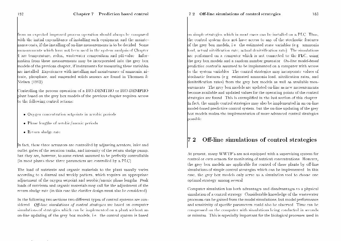
��� Chapter �� Prediction based control
from an expected improved process operation should always be compared
with the initial expenditures of installing such equipment and the mainte�
nance costs if the installing of on�line measurements is to be decided� Some
measurements which have not been used in the system analysis of Chapter
� are temperature redox wastewater composition and pH�value� Infor�
mation from these measurements may be incorporated into the grey box
models of the previous chapter if instruments for measuring these variables
are installed� Experiences with installing and maintenance of ammonia ni�
trate phosphate and suspended solids sensors are found in Thomsen
Nielsen �������
Controlling the process operation of a BIO�DENITRO or BIO�DENIPHO
plant based on the grey box models of the previous chapter requires access
to the following control actions�
� Oxygen concentration setpoints in aerobic periods�
� Phase lengths of aerobic�anoxic periods�
� Return sludge rate�
In fact these three actuators are controlled by adjusting aerators inlet and
outlet gates of the aeration tanks and intensity of the return sludge pump
but they are however to some extent assumed to be perfectly controllable
�in most plants these three parameters are controlled by a PLC��
The load of nutrients and organic materials to the plant usually varies
according to a diurnal and weekly pattern which requires an appropriate
adjustment of the oxygen setpoint and aerobic�anoxic phase lengths� Peak
loads of nutrients and organic materials may call for the adjustment of the
return sludge rate �in this case the clari�er design must also be considered��
In the following two sections two di�erent types of control systems are con�
sidered� O�line simulations of control strategies are based on computer
simulations of strategies which can be implemented on a plant without an
on�line updating of the grey box models i�e� the control system is based
��� O� line simulations of control strategies ���
on simple strategies which in most cases can be installed on a PLC� Thus
the control system does not have access to any of the stochastic features
of the grey box models i�e� the estimated state variables �e�g� ammonia
load actual nitri�cation rate actual denitri�cation rate�� The simulations
are performed on a computer which is not connected to the PLC using
the grey box models and a random number generator� Online modelbased
predictive control is assumed to be implemented on a computer with access
to the system variables� The control strategies may incorporate values of
stochastic features �e�g� estimated ammonia load nitri�cation rates and
denitri�cation rates� from the grey box models as well as available mea�
surements� The grey box models are updated on�line as new measurements
become available and updated values for the operating points of the control
strategies are found� This is exempli�ed in the last section of this chapter�
In fact the simple control strategies may also be implemented in an on�line
model�based predictive control system but the on�line updating of the grey
box models makes the implementation of more advanced control strategies
possible�
��� O��line simulations of control strategies
At present many WWTP�s are not equipped with a supervising system for
control or even sensors for monitoring of nutrient concentrations� However
the grey box models are applicable for control of these plants by o��line
simulations of simple control strategies which can be implemented� In this
case the grey box models only serve as a simulation tool to choose one
optimal strategy among several�
Computer simulation has both advantages and disadvantages to a physical
simulation of a control strategy� Considerable knowledge of the wastewater
processes can be gained from the model simulations but model performance
and sensitivity of speci�c parameters could also be observed� Time can be
compressed on the computer with simulations being conducted in seconds
or minutes� This is especially important for the biological processes used in
� �

��� Chapter �� Prediction based control
wastewater treatment where rates are relatively slow and physical experi�
mentation may require weeks or even months� Computer simulations are
done easier cheaper and faster than physical experimentation and in the
case of wastewater treatment it is also more hygienic� The disadvantages
are that the computer simulations are no better than the model and data
they are based on and if the model is not a reasonable representation of
the WWTP computer simulations result in the generation of large quanti�
ties of worthless results� In particular the simulation of control strategies
bringing the system into a state which has not been used for estimating the
model may lead to fatal conclusion regarding the control of the system� As
a general rule computer simulations should at �rst be used for validating
the model structure and secondly to choose the optimal control strategy
to be used in a physical experiment�
Assuming that the oxygen concentration and the suspended solids concen�
tration in the aeration tanks are perfectly controlled according to their
setpoints the grey box models of Section ��� represent a simulation tool
for o��line testing of control strategies� The required input �ow rate to the
grey box models can be simulated using a sinusoidal signal or a time series
of historic �ow rates may be applied� The grey box models have the advan�
tage to other models that the process parameters used for simulation are
estimated on actual data from the given plant� However there are some
limitations to the use of the grey box models in simulations� The models
may not be appropriate of simulating load situations which are not re�ected
in the data set used for estimation� Thus the parameter estimation of the
grey box models should be based on data with highly time�varying loads�
The control strategies proposed below are simple strategies which can be
implemented on a PLC without an on�line use of the grey box models�
More advanced strategies are proposed in the next section�
For the control of the oxygen concentration setpoint the following o��line
control strategies are proposed�
��� A constant oxygen concentration setpoint�
��� O� line simulations of control strategies ���
��� A sinusoidal oxygen concentration setpoint which is a linear function
of the estimated diurnal variation of the in�uent ammonia load rate
�������
and for the control of aerobic and anoxic phase lengths�
�a� Constant phase lengths�
�b� Switching o� the aeration once the ammonia concentration in the
aerobic period lies below a certain value e�g� �� mg NH �N�l�
�c� The strategy �b� combined with switching of phases once the nitrate
concentration lies below a certain value e�g� �� mg NO�� �N�l�
The strategies listed above are only examples of a vast number of strategies
that can be simulated o��line� Strategies for control of the return sludge
rate are not proposed because the simulation of such strategies using the
grey box models would not take the in�uence on the clari�ers into account�
Raising the return sludge rate results in higher suspended solids concentra�
tions in the aeration tanks yielding higher removal rates of nutrients but
it also increases the likelihood of activated sludge loss to the e�uent�
The di�erent control strategies are evaluated by a cost function which may
incorporate the cost of aeration switching of phases return sludge pump�
ing and the discharge of ammonia nitrate and phosphate to the e�uent
assuming that the concentration of dissolved nutrient salts is unchanged by
passage of the clari�er� While the costs of the operations on the plant can
be calculated in terms of money the discharge of nutrients does not have
an immediate cost related to it unless regulatory limits of discharge are
exceeded� A cost function of the type illustrated in Figure ��� may prove
appropriate where !� is the additional cost of discharging an additional
� mg�l below the discharge limit ! is the additional cost of discharging
an additional � mg�l above the discharge limit and is the cost of ex�
ceeding the regulatory limit� The values of !� ! and may be chosen
according to the expected e�ects of nutrient discharge on the e�uent and
in lack of such knowledge appropriate values are chosen�
� �

��� Chapter �� Prediction based control
����������
��������������
��
�
�
E�uent
��Concentration
Regulatory
limit
Cost per volume
��
��
Figure ���� Suggested cost function for the discharge of nutrients� !� and
! are the additional costs per volume of discharging an additional � mg�l
below and above the regulatory discharge limit�
O��line simulations of the grey box models may also be applied to WWTP�s
without on�line sensors permanently installed if data can be sampled from
the plant in a representative period using a mobile measuring equipment�
These data are used to estimate the grey box models for the given plant and
o��line simulations of strategies which are possible based on the perma�
nently available information at the plant are performed� This optimization
of the existing control system applies to smaller plants where the costs of
installing on�line sensors may exceed the bene�ts of improved operation�
��� On line model based predictive control ���
The grey box models also represent a tool which can be used for assess�
ing the e�ect of operational strategies regarding the biomass activity �both
autotrophic and heterotrophic�� If an extensive data set is monitored dur�
ing the physical experiment of improving the overall biomass activity the
parameter estimates of the maximum nitri�cation rate and maximum de�
nitri�cation rate are statistics by means of which an improvement can be
recognized assuming that external variables in�uencing the biomass activ�
ity �e�g� temperature wastewater composition pH�value� are constant or
somehow compensated for� For instance the e�ect of adding ferrosulphate
and other iron salts for chemical precipitation on the biomass activity may
be assessed�
��� On�line model�based predictive control
Assuming that the WWTP is equipped with a SCADA�system �Supervi�
sion Control And Data Acquisition� such that a data�interchange between
the on�line measurements an on�line model and the actuators is possible�
In this case the grey box models of Section ��� provide an optimal on�line
estimation ��ltering� of the monitored nutrient concentrations using the
Kalman �lter and on�line predictions of nutrient concentrations are ob�
tained which can be used for prediction based control� Employing on�line
predictions in the operation control is advantageous because the on�line
measurements of nitrate phosphate and especially ammonia concentra�
tions are associated with time delays due to the �ltering of the sample and
the composition analysis� At present the time delays in the commercial
monitoring systems of nutrient salt concentrations are of the magnitude ��
�� minutes while the time delay of the monitoring systems for oxygen and
suspended solids concentrations are considerably less� This means that the
operation control strategies can be e�ectuated more precisely when predic�
tions are applied thereby resulting in an improved operation performance�
Furthermore on�line updating gives access to the stochastic features of
the grey box models �e�g� estimated ammonia loads nitri�cation rates
denitri�cation rates� which can be used for developing control strategies�
� �

��� Chapter �� Prediction based control
The implementation of a control strategy in an on�line model�based pre�
dictive control system di�ers signi�cantly from the implementation of an
o��line simulated control strategy in the way the controlling actions are
e�ectuated� While the methods of the previous section are associated with
the assessment of the measured values �e�g� switching o� the aeration when
the measured ammonia concentration lies below �� mg NH �N�l� the con�
trolling actions of a model�based predictive control system are associated
with the assessment of the predictions and estimates using their distribu�
tions �e�g� switching o� the aeration when the ���minutes ahead prediction
of the ammonia concentration lies below �� mg NH �N�l with a probabil�
ity of �"�� In the following the control strategies which are presented
are based on predictions at time of operation i�e� the time delays of the
sensors are incorporated in the predictions�
The information obtained from the grey box models can be used to develop
more advanced controlling strategies in addition to those proposed in the
previous section� For the control of the oxygen concentration setpoint the
following additional on�line strategy is proposed�
��� An adjustment of the oxygen concentration setpoint proportional to
the predicted nitri�cation rate �brnit�NH��
�t or brnit�NO��
�t� at time of
operation�
and for the control of the aerobic and anoxic periods�
�d� Switching from the aerobic to the anoxic phase when brnit���t �
where � is an appropriately chosen constant and rnit���t is the pre�
dicted nitri�cation rate at time of operation� This strategy corre�
sponds in principle to strategy �b� with the major di�erence being
that this strategy uses a stochastic feature from the grey box models
in the evaluation of the plant operation�
�e� Switching from the aerobic to the anoxic phase when brnit���t brdenit�t
where brnit���t is the predicted nitri�cation rate at time of operation
and brdenit�t is the predicted denitri�cation rate obtained from the
��� On line model based predictive control ���
Aerobic ��
anoxic
�
�
Anoxic �� aerobic
Area of operation
brnit���t
brdenit�t � brnit���t
brnit���t brdenit�tbrdenit�t
Figure ���� Illustration of the feasibility area of operation strategy �e�� At
each timestep the operation point �brnit�t� brdenit�t� is plotted� and if it is
outside the operation area� the phases are switched� The operation of the
plant will move from lower boundary to upper boundary and reverse in an
alternating manner�
present operating conditions if the switching is performed� Simi�
larly switching from the anoxic phase to the aerobic phase whenbrdenit�t �brnit���t where brdenit�t is the predicted denitri�cation rate
at time of operation and brnit���t is the predicted nitri�cation rate
obtained from the present operating conditions if the switching is
performed� Thus the potential removals of ammonia and nitrate are
compared at every time step using � and which are appropriately
chosen constants� Figure ��� shows the feasibility area of this strategy
where the present operating conditions of the plant are maintained as
long as the operation point �brnit���t brdenit�t� is within the boundaries
of the operation area�
� �
�� Chapter �� Prediction based control
The listing above only represents examples of the innumerable possible
on�line model�based control strategies� The strategies for phase control of
the BIO�DENITRO and BIO�DENIPHO processes presented above only
include the main phases of these processes �the lengths of the aerobic and
anoxic periods in the operation cycle i�e� Phase A and C in Figure ��� and
Phase B in Figure ����� Including the control of in�uent and e�uent �ow
from the alternating tanks in the strategies yields many new alternatives�
Selection of the most appropriate on�line model�based predictive control
strategy is primarily performed by o��line simulations of the wastewater
processes and the plant operation evaluated by a cost function as described
in the previous section� Secondly a physical implementation of the control
strategy may be performed to validate the e�ect of the given strategy�
Furthermore implementing the grey box models on�line in the SCADA�
system occurrences of inhibition and toxicity may be detected by contin�
uously assessing the estimated maximum nitri�cation rate and maximum
denitri�cation rate� In this case the grey box models serve the function of
surveillance� In addition automatic strategies or alarming the personnel
are employed in order to minimize the e�ect of inhibition and toxicity� Pro�
cedures for detection of failures in the measuring equipment for nutrient
salt concentrations are also easily applied due to the grey box models� For
example if the last three measurements of the ammonia concentration lies
outside the ��" con�dence limits of the predicted values the ammonia sen�
sor is most likely mis�functioning� However scaling and o�set calibration
errors are more di�cult to detect unless two sets of the same measure or
estimate can be compared� For example if both alternating aeration tanks
are equipped with ammonia sensors the results of estimating the grey box
models on both time series should correspond reasonably with allowances
to the uncertainty of the estimates�
��� A simulation study ���
��� A simulation study
In order to investigate the strategies proposed in the two previous sections
the grey box models of Section ��� are used for simulating a full�scale plant
with variable loads and nitrogen removal rates� A biological nutrient re�
moval system consisting of two alternating tanks �each having a volume of
��� m�� is simulated using parameter values which are estimated on a
large data set from the Aalborg West WWTP �see Chapter ��� Throughout
the simulation a constant suspended solids concentration of ��� g SS�l is
maintained in the aeration tanks� A total of � days �starting with a Mon�
day� without any excessive disturbances from rainfall events is simulated�
The load of wastewater entering the biological nutrient removal system is
simulated using a diurnal pro�le in the form of a Fourier expansion �������
This pro�le has been estimated on historic data fromAalborgWest WWTP�
The average in�uent �ow to the aeration tanks �i�e� the raw wastewater
mixed with returned activated sludge� is � m��h on weekdays and �
m��h on weekends� The load of ammonia to the plant is simulated using
������ and ����������� with the parameter estimates from the last column
of Table ���� In a similar way the nitri�cation denitri�cation and nutrient
transport processes are simulated by use of the appropriate equations of
Section ��� with the parameter estimates found in Tables ��� ��� ���
and ���� All the simulations in this section are excited by the same noise
sequence for generating the innovations of the grey box models�
����� The cost function
The control strategies proposed previously �strategies ������� for control of
the oxygen setpoint concentration and strategies �a���e� for control of the
aerobic and anoxic phase lengths� are evaluated against each other using
the cost function for the discharge of nutrients sketched in Figure ��� and
a cost function of aerating the activated sludge� Furthermore in order to
� �

��� Chapter �� Prediction based control
compare the control strategies to the typical time scheduling of the BIO�
DENIPHO process at Aalborg West WWTP this plant operation is also
simulated and evaluated by the same cost function�
In the present example the cost of discharging ammonia and nitrate to
the recipient when e�uent concentrations are below regulatory limits is
respectively
!�NH��
�� DKK�kg NH �N
!�NO��
�� DKK�kg NO�� �N
The cost of discharging ammonia and nitrate to the recipient when e�uent
concentrations are above regulatory limits is respectively
! NH��
�� DKK�kg NH �N
! NO��
�� DKK�kg NO�� �N
and the cost of exceeding the regulatory limits at any time is
�NH��
�� DKK�� m�
�NO��
�� DKK�� m�
The regulatory discharge limits for the ammonia and total nitrogen concen�
trations are ��� mg NH �N�l and �� mg N�l in the majority of receiving
waters in Denmark today� However since the organic nitrogen concentra�
tion in the e�uent is not known it is assumed that approximately ����"
of the total nitrogen in the e�uent is organicly bound� Hence if the com�
bined inorganic nitrogen concentration in the e�uent exceeds �� mg�l an
additional cost on the nitrate concentration can be added to the cost func�
tion� Furthermore it is assumed that e�uent concentrations of ammonia
and nitrate from the aeration tanks remain unchanged by passage of the
clari�er into the recipient i�e� there are no signi�cant nitrogen removal
processes taking place in the clari�er� Thus a cost function of discharging
ammonia may be formulated
��� A simulation study ���
CostNH��
�t ���������������������
!�NH��
� SENH��
�t�Qt
if SENH��
�t� �limit�NH�
�
!�NH��
� �limit�Nh��
� Qt � �NH��
�Qt
�! NH��
� �SENH��
�t� �limit�NH�
�
� �Qt
if SENH��
�t� �limit�NH�
�
�����
where �limit�NH��
��� mg NH �l and similarly for the discharge of ni�
trate
CostNO��
�t ���������������������
!�NO��
� SENO��
�t�Qt
if SENH��
�t� SENO��
�t� �limit�Ninorganic
!�NO��
� �limit�Ninorganic
� Qt � �NO��
�Qt
�! NO��
� �SENH��
�t� SENO��
�t� �limit�Ninorganic� �Qt
if SENH��
�t� SENO��
�t� �limit�Ninorganic
�����
where �limit�Ninorganic
�� mg N�l� The superscript E in ����� and �����
indicates that the e�uent concentration of ammonia and nitrate to the
recipient are equal to the ammonia and nitrate concentrations in the alter�
nating tank with e�uent �ow�
The cost parameters for discharge of nitrogen are adequately chosen with
respect to the estimated cost of removing ammonia and nitrate in a WWTP
and expected causal e�ect on the ecological system of the recipient� How�
ever the choice of these cost parameters for the discharge of nutrients to
the recipient should be addressed to the local authorities and the politi�
cians i�e� the people with the power to decide if advanced on�line control
should be implemented on the municipal plants�
� �

��� Chapter �� Prediction based control
The cost of aerating may be easily derived if a model for the oxygen setpoint
concentration as a function of rotor RPM and plant load is given� However
such a relationship has not been identi�ed in the present context but it has
been estimated at the Aalborg West WWTP that the cost of aerating � kg
NH �N is approximately � DKK� It is assumed that the cost of aerating
is not simply related to the removal of ammonia but that this cost is
related to maintaining the activated sludge aerated� Thus the following
cost function of aerating may be appropriate
CostO� �t � DKK�kg N � kload�NH��
�f �Qt � V �
O��saturation
O��saturation�O��setpoint
�����
where O��saturation � mg O��l is the saturation constant for oxygen
and kload�NH��
�f � Qt � V is the actual mass load of ammonia to the plant
at time t� The last term in ����� describes the e�ciency of the aerating
equipment as a function of the oxygen setpoint concentration O��setpoint�
Hence the cost of aerating is assumed to be proportional to the ammonia
load of the given operation cycle and a term for aerating according to the
oxygen setpoint concentration of the control strategy� The cost function
above ����� is likely to overestimate the actual cost of aerating since the
cost of keeping the activated sludge aerated is lower than the cost of both
removing ammonia and keeping the activated sludge aerated� However in
the present simulation study ����� is only used for exemplifying the concept
of prediction based control�
In the present simulations example the total cost of operation is related to
nitrogen discharge and aeration which is found as follows�
Costtotal �� X
t��CostNH�
�
�t � CostNO��
�t � CostO� �t �����
The time�step in the simulation is set to � minutes which gives a total of
�� observations�
��� A simulation study ���
The parameters values used in the cost functions above and the behavior of
the cost functions may be disputed� However the key issue of the present
simulation study is not addressed to the derivation of exact savings by im�
plementing on�line model�based predictive control but it is addressed to
an internal evaluation of the proposed control strategies and the demon�
stration of the advantages using estimated grey box models for evaluating
and improving control strategies� Thus if the cost functions and related
parameters could be determined more exactly �e�g� in the form of a po�
litical decision� better estimates on the savings of implementing advanced
control strategies can be found� Finally other costs related to the plant
operation such as excess sludge disposals the number of times the aerating
equipment is turned on electricity consumption for controlling gates etc�
may be also taking into account when the total costs of di�erent control
strategies are considered�
����� Simulation results
The typical time scheduling of the BIO�DENIPHO process at the Aalborg
West WWTP is similar to the scheme in Figure ��� with the exception
of Phase C being omitted� The total operation cycle length is normally
� hours and the duration of Phase A and Phase B are � minutes and
� hour � minutes respectively� Applying ����� to a ten days simulation
of this BIO�DENIPHO operation mode results in a total cost of �����
DKK� In Table ��� the total costs of simulated operations are given for
the combination of the proposed control strategies of the oxygen setpoint
concentration ������� and the aerobic�anoxic phase lengths �a���e�� Below
the cost values in the table the total cost relative to the typical BIO�
DENIPHO time scheduling given above is listed� The operation of the
plant in the simulations has been optimized with respect to the parameters
of the control strategies� In most cases the optimization can only be done
by hand since the total cost function is not smooth due to the randomly
generated innovations used in the simulations� Hence a global optimum is
not guaranteed in all cases and the costs found in Table ��� act more as
possible improvements�
� �

��� Chapter �� Prediction based control
Control strategies for Oxygen setpoint concentration
Aalborg West WWTP strategies
Typical operation ��� Constant ��� Sinusoidal ��� Oxygen set�
����� DKK oxygen oxygen point function
�" setpoint setpoint of brrnit�t
�a� Constant ����� DKK ���� DKK ���� DKK
phase lengths ���" ���" ���"
�b� Switching o� ���� DKK ���� DKK ���� DKK
aeration SNH��
�t� ���" ���" ���"
�c� Combined with ����� DKK ����� DKK ����� DKK
switching SNO��
�t� ����" ����" ����"
�d� Aerobic � anoxic ����� DKK ����� DKK ����� DKKbrnit���t � ����" ����" ����"
�e� Strategy sketched ����� DKK ���� DKK ���� DKK
in Figure ��� ���" ����" ����"
Table ���� Lattice of control strategies evaluated by the cost function
given in the previous subsection� The typical timescheduling of the BIO
DENIPHO process results in a total cost of ���� DKK�
Comments to the simulation results in Table ����
�a��� The time scheduling of the BIO�DENIPHO process is optimized with
respect to the phase lengths and the oxygen setpoint concentration�
In this case the length of the total operation cycle is � hours with
� minutes for Phase A and �� minutes for Phase B in Figure ����
The typical time�scheduling is � minutes for Phase A and � hour
� minutes for Phase B� The optimal oxygen setpoint concentration
is found to be ��� mg O��l which is lower than the typical oxygen
setpoint concentration� Thus a signi�cant improvement of the total
cost is obtained compared to the typical BIO�DENIPHO operation
mode simply by optimizing the present plant operation�
��� A simulation study ���
�a��� Phase lengths are as in �a��� The oxygen setpoint concentration is
controlled according to the ammonia load pro�le with an average
of ��� mg O��l and it varies within the range of ������ mg O��l�
Compared to strategy �a�� this strategy yields a lower oxygen con�
sumption for aeration and a slight improvement in the total cost�
�a��� Phase lengths are as in �a��� The oxygen setpoint concentration is
optimized as a suggested linear function of the present nitri�cation
rate i�e� O��setpoint ��� � �� � brnit�NH��
�t� Hence the oxygen
setpoint concentration is approximately within ������ mg O��l in
the beginning of the aerobic phase whereupon it decreases towards
��� mg O��l� Compared to strategy �a�� a small improvement of the
total cost is found�
�b��� Phase lengths are as in �a�� with the aerating equipment being turned
o� in the aerobic phase once the measured ammonia concentration
SNH��
�t ��� The time delay on the ammonia concentration mon�
itoring equipment is �� minutes and the optimal oxygen setpoint
concentration is found to be ��� mg O��l� Hence when the aeration
is turned o� the actual ammonia concentration in the aeration tank
is approximately �� mg NH �N�l� A signi�cant improvement of the
total cost compared to strategy �a�� is obtained� It should also be
noted that the optimal oxygen setpoint concentration is increased�
�b��� Phase lengths are as in �a�� with the aerating equipment being turned
o� in the aerobic phase once the measured ammonia concentration
SNH��
�t ���� The optimal oxygen setpoint concentration is found
to vary within the range of ������� mg O��l according to the diurnal
pro�le of the ammonia load� However the total cost of this strategy
does not di�er signi�cantly from the value obtained in �b���
�b��� Phase lengths are as in �a�� with the aerating equipment being turned
o� in the aerobic phase once the measured ammonia concentration
SNH��
�t ��� The oxygen setpoint concentration is optimized as
a linear function of the present nitri�cation rate O��setpoint ��� �
�� �brnit�NH��
�t but this does not give an improved total cost for this
strategy compared to �b���
� �

��� Chapter �� Prediction based control
�c��� A switch of operating conditions from the aerobic to anoxic phase
is performed when SNH��
�t ��� and similarly from the anoxic to
aerobic phase if SNO��
�t �� or SNH��
�t � ���� In the simulation
of control strategy �c� a minimum aerobic phase of �� minutes is al�
ways ensured� The time delay of the nitrate concentration monitoring
equipment is � minutes and the optimal oxygen setpoint concentra�
tion is found to be ��� mg O��l� Compared to strategy �b�� a notable
improvement in the total cost of operation is achieved�
�c��� A switch of operating conditions from the aerobic to anoxic phase
is performed when SNH��
�t ��� and similarly from the anoxic to
aerobic phase if SNO��
�t ��� or SNH��
�t � ���� The optimal oxy�
gen setpoint concentration is found to vary within the range �������
mg O��l according to the diurnal pro�le of the ammonia load� No
signi�cant further improvement of the total cost is obtained�
�c��� A switch of operating conditions from the aerobic to anoxic phase
is performed when SNH��
�t ��� and similarly from the anoxic to
aerobic phase if SNO��
�t ��� or SNH��
�t � ���� The oxygen setpoint
concentration is optimized as O��setpoint ���� �� � brnit�NH��
�t� No
signi�cant improvement of the total cost is obtained�
�d��� Phase lengths are as in �a�� with the aerating equipment being turned
o� in the aerobic phase once the model�based estimate of the ni�
tri�cation rate brnit�NH��
�t ���� The optimal oxygen setpoint
concentration is found to be ��� mg O��l� This strategy compares
to �b�� in its operation behavior and it is clearly recognized that the
use of on�line estimates in the plant control improves the total cost
of operation�
�d��� Phase lengths are as in �a�� with the aerating equipment being turned
o� in the aerobic phase once the model�based estimate of the ni�
tri�cation rate brnit�NH��
�t ���� The optimal oxygen setpoint
concentration is found to vary within the range ������� mg O��l ac�
cording to the diurnal pro�le of the ammonia load� The total cost
of this strategy is somewhat lower than the costs of �d�� and �d��
though the reason is still unclear�
��� A simulation study ���
�d��� Phase lengths are as in �a�� with the aerating equipment being turned
o� in the aerobic phase once the model�based estimate of the nitri�
�cation rate brnit�NH��
�t ���� The oxygen setpoint concentration
is optimized as O��setpoint ��� � �� � brnit�NH��
�t� No signi�cant
improvement of the total cost is obtained�
�e��� The strategy is sketched in Figure ��� where switching from aerobic
to anoxic conditions is performed when brnit�NH��
�t �����brdenit�t and
where switching from anoxic to aerobic conditions is performed whenbrdenit�t �� � brnit�NH��
�t� The nitri�cation and denitri�cation rates
used in this strategy are on�line estimates from the grey box models�
The optimal oxygen setpoint concentration is found to be ��� mg
O��l� This strategy compares to �c�� in its operation behavior and
for this type of strategy it is also clearly recognized that the use of
on�line estimates in the control strategy improves the total cost of
operation�
�e��� The strategy is sketched in Figure ��� where switching from aerobic
to anoxic conditions is performed when brnit�NH��
�t �����brdenit�t and
where switching from anoxic to aerobic conditions is performed whenbrdenit�t ����brnit�NH��
�t� The optimal oxygen setpoint concentration
is found to vary within the range ������� mg O��l according to the
diurnal pro�le of the ammonia load� This control strategy yields the
minimum total cost of operation in the table�
�e��� The strategy is sketched in Figure ��� where switching from aerobic
to anoxic conditions is performed when brnit�NH��
�t ���� � brdenit�t
and where switching from anoxic to aerobic conditions is performed
when brdenit�t ��� � brnit�NH��
�t� The oxygen setpoint concentration
is optimized as O��setpoint ��� � ��� � brnit�NH��
�t� No signi�cant
improvement of the total cost is obtained�
The optimal parameters of the control strategies above are found by sim�
ulating a �nite number of parameter combinations in a discrete parameter
space �e�g� combinations of ������ mg O��l with a step length of �� mg
O��l are performed for the oxygen setpoint concentration�� Hence the
� �

� Chapter �� Prediction based control
strategies above may be further optimized with respect to the parameters
if the sensitivity of the parameter space is increased� However this will
also increase the number of simulations to be performed�
����� Discussion
The total cost of plant operation seems to be almost indi�erent to the
proposed strategies for control of the oxygen setpoint concentration as the
level of complexity in the proposed strategies for control of aerobic�anoxic
phase lengths increases� At the same time the oxygen setpoint concentra�
tion is increased� Hence according to this simulation example the plant
should be operated at a high oxygen setpoint concentration with relative
short aerobic periods� Actually using di�erent parameter values in the
cost functions above ��������� it is found that the optimal oxygen setpoint
concentration is determined by the cost of aerating relative to the cost of
discharging ammonia to the recipient �e�g� if the cost of discharging am�
monia is increased�decreased the optimal oxygen setpoint concentration is
also increased�decreased��
The phase lengths of the aerobic and anoxic periods are mainly determined
by the cost of discharging ammonia relative to discharging nitrate� How�
ever the simulations show that at least �" of the operation time should
always be dedicated to denitri�cation in the more advanced control strate�
gies ��b���e�� and aerobic periods should never coincide with periods of
in�uent �ow�
The strategy minimizing the total cost of operation in Table ��� is found
to be �e�� which yields a slightly improved total cost compared to �e���
Comparing this strategy with the typical plant operation of Aalborg West
WWTP the following average e�uent concentrations are obtained for the
ten days simulation�
��� A simulation study ��
Typical operation Strategy �e��
SE
NH��
��� mg NH �N�l ��� mg NH �N�l
SE
NO��
���� mg NO�� �N�l ���� mg NO�� �N�l
While the average e�uent ammonia concentration is slightly increased by
applying strategy �e�� the average e�uent nitrate concentration is almost
reduced by � mg NO�� �N�l� Furthermore the simulation of the control
strategy �e�� yields ��" aerobic operation time at an average oxygen con�
centration of ��� mg O��l and ��" anoxic operation time� The typical plant
operation has �" aerobic operation time at an oxygen concentration of
�� mg O��l� Thus evaluating these two di�erent plant operations only by
the cost of aeration it is foundTypical operation Strategy �e��
CostO��total ���� DKK ����� DKK
Therefore strategy �e�� reduces the total nitrogen discharge to the recip�
ient as well as the cost of aerating� It should be stressed that the major
improvement in the total cost function of the di�erent strategies compared
to the typical operation is obtained from the identi�cation of the nitrogen
removal processes while the optimization of the parameters of the control
strategy has a smaller e�ect on the total cost function�
If the cost function ����� is an adequate measure of plant performance a
plant operated according to the control strategy �e�� can be reduced in
size� It is found that a reduction of the volumes of the aeration tanks
in the simulation of control strategy �e�� to ��� m� yields a total cost
of operation similar to the typical plant operation� This is a reduction
in volume of ���"� Thus if control strategies for plant operation are
taken into account when designing new plants large savings on the cost of
construction may be obtained�
� �

�� Chapter �� Prediction based control
��� Conclusion
In this chapter methods are proposed which use the grey box models of the
previous chapter for control of the BIO�DENITRO and BIO�DENIPHO
processes� Applying the grey box models to a WWTP requires in general
that the �ow rate oxygen ammonia nitrate phosphate and suspended
solids concentrations are monitored and used for estimating the parameters
of the given plant� Lack of some of these measurements result in less
appropriate models and a reduced operation performance� The grey box
models may be used for control of the oxygen concentration setpoints in
aerobic periods and phase lengths of aerobic and anoxic periods� Two
di�erent approaches to the application of the grey box models in control
of WWTP�s are suggested� o��line simulations of control strategies and
on�line model�based predictive control�
In order to use the grey box models for control of plant operation strategies
for the given actuators needs to be developed� If these strategies and a cost
function for evaluating the strategies are supplied the grey box models may
serve as an o��line simulator by means of which the e�ect of the di�erent
strategies can be assessed� The cost function may incorporate the costs
of plant operation and a cost related to the discharge of nutrients to the
recipient� Furthermore the rates estimates of the grey box models may be
used for assessing the e�ects of physical experiments related to the biomass
activity�
Implementing the grey box models on�line in a SCADA�system provides
on�line �ltering of the monitored nutrient salts concentrations and on�line
predictions of the nutrient concentrations� Applying model predictions
to the controlling system enhances the operation performance because the
measurement system is associated with noise and some time delay and more
advanced control strategies may be proposed based on estimates from the
models in addition to strategies based on measured values� Furthermore
the implementation of the grey box models on�line serve as a surveillance
system for inhibition and toxicity� Failures and mis�calibrations of the
��� Conclusion ��
measurement system can be detected if some kind of rule�based procedures
on the parameter estimates and model predictions are applied�
In a simulation study strategies for control of the oxygen concentration
setpoint and aerobic�anoxic phase lengths are evaluated by a cost function�
The grey box models with parameters estimated on data from the Aalborg
West WWTP are used for simulating the BIO�DENIPHO process� The
simulations show that a reduction in both total nitrogen discharge and
oxygen consumption is obtained by applying advanced control strategies
to the plant operation� However the major improvement in the total cost
function of the di�erent strategies compared to the typical operation is
obtained from the identi�cation and quanti�cation of the ammonia load
nitri�cation and denitri�cation processes� This may have a major impact
on the plant operation of existing plants as well as the design of new plants�
� �

�� Chapter �� Prediction based control
Chapter
Conclusion
The present thesis is addressed to the formulation of operational models for
control of wastewater treatment plants including nutrients removal� The
proposed models are from a pragmatically point of view based on the avail�
able data of the given plant being modelled� Physical insight of the system
is incorporated into the models by including terms of the hydraulic and
biological processes which can be statistically identi�ed� These terms are
discrete time approximations to the deterministic di�erential equation for�
mulations which have been predominant in the modelling of wastewater
processes in the last decades�
Measurements of ammonia nitrate and phosphate concentrations from
plants of the BIO�DENITRO and BIO�DENIPHO type contain a great deal
of dynamic due to the alternating operation mode� An excessive amount of
information is extracted from the large variations of these measurements
making the statistical identi�cation of rates from several hydraulic and
biological processes possible� The models in the present context include
rate expressions for
� In�uent nutrient load�
��
� �

�� Chapter �� Conclusion
� Nutrient transport of the aeration tanks�
� Hydrolysis and growth of biomass�
� The nitri�cation process�
� The denitri�cation process�
� Biological phosphate uptake in biomass�
� Stripping of phosphate�
The majority of parameters used for modelling these processes have the
quality of interpretability relating to the deterministic theory of the pro�
cesses� The alternating operation mode introduces natural break points in
the time series of the measurements which is used for modelling of three
time�varying parameters in the operation cycle time domain�
� In�uent load rate of ammonia�
� Maximum nitri�cation rate�
� Maximum denitri�cation rate�
Applying simple approximations to the three time�varying parameters above
estimates of these describe the variations of the in�uent ammonia con�
centration to the aeration tanks the activity of the autotrophic biomass
and the activity of the heterotrophic biomass� The three time�varying pa�
rameters are essential to the nitrogen removal performance of a biological
nutrient removal system� The models presented in this thesis are denoted
grey box models since they are not as detailed as the #white# determinis�
tic models and still contain some physical insight of the system as opposed
to the black box models� Data from two di�erent wastewater treatment
facilities have been used for the development of the grey box models�
Two data sets from the Lundtofte pilot scale plant have been employed for
the estimation of the grey box models� In order to use the Kalman �lter
Chapter �� Conclusion ��
on this data a model for the correlation of the measurement noise has to
be formulated� It is found that the identi�cation of Monod�kinetic expres�
sions is practically feasible if an extensive data set is available� The kinetic
parameter estimates of the grey box models are consistent with the values
found in the literature� The estimated in�uent ammonia concentrations
re�ect a major part of the dynamics of the measured in�uent ammonia
concentrations but the estimates are biased towards lower values� The
variations of the in�uent ammonia concentrations are modelled according
to human behavior in the operation cycle time domain but the diurnal
and weekly patterns are interrupted by periods of rainy weather� The ac�
tivities of the autotrophic and the heterotrophic biomass are time�varying�
However lack of information on external variables describing some of this
variation reduces the performance of the models in the operation cycle time
domain�
At the Aalborg West wastewater treatment plant two sets of ammonia and
nitrate concentrations are monitored from the alternating aeration tanks�
The modelling of the in�uent ammonia load to the plant is divided into
two distinct situations dry weather periods and rainy weather periods�
The latter is based on the assumption that the dynamics of the sewerage
the primary clari�ers and anaerobic pretreatment tanks can be modelled
as two ideally mixed tanks in series with identical volume holdings� The
estimates of the kinetic parameters are consistent with the suggested val�
ues of the literature though several of these estimates are in�uenced by
the mis�calibration of one of the ammonia sensors� The estimated in�u�
ent ammonia concentrations show large variations which are partly due to
many rainy weather periods� The estimated autotrophic biomass activity
is found to be strongly correlated with past estimates of the ammonia load
rate� This is modelled as a short�term dependency in the operation cycle
time domain� However the slow dynamics of the autotrophic and the hete�
rotrophic biomass are not adequately described in the operation cycle time
domain due to lack of information on the in�uence of external variables�
A small number of irregularly samples measurements of temperature and
sludge volume index may suggest a relationship between these two variables
and the overall biomass activity�
� �

�� Chapter �� Conclusion
The models are useful for on�line surveillance and control of a wastewater
treatment plant of the BIO�DENITRO or BIO�DENIPHO type because
the states of the plant are quanti�ed by the physically interpretable pa�
rameters of the grey box models� In order to use the grey box models
for control operational strategies need to be developed� These strategies
are evaluated by a cost function which includes the cost of operation and
discharge of nutrients� Primarily the grey box models may be applied
to o��line simulations of the developed strategies and secondly selected
strategies may be practically implemented on the plant with or without
an on�line implementation of the grey box models� A simulation study
evaluating and optimizing several control strategies shows that a reduc�
tion in both total nitrogen discharge and oxygen consumption is obtained
by applying on�line model�based predictive control to the plant operation�
Though the identi�cation and quanti�cation of the wastewater processes
used in the control strategies has a larger e�ect on the plant operation
than the optimization of the parameters of the control strategies� Thus an
improved operation by applying advanced control should be considered on
existing plants as well as in the design of new plants�
Appendix A
Numerical considerations
The choice of numerical methods applied to the estimation of the grey box
models presented in Chapter � is crucial� The increasing complexity of the
parameterization of the structural models calls for the development of well�
suited numerical methods in order to implement the estimation algorithms
on a computer� The problems arise due to the �nite arithmetic in a com�
puter introducing rounding errors for every calculation with real numbers�
The calculations of an algorithm may have several algebraically equiva�
lent implementations with di�erent numerical properties� Thus for a given
estimation algorithm the selection of the appropriate numerical implemen�
tation is very important� However as a general rule the computations
should always be carried out using double precision� In the �rst section of
this appendix methods for stabilizing the Kalman �lter recursions given in
Section ��� are described and the second section deals with the numerical
optimization�
��
� �

�� Appendix A� Numerical considerations
A�� Kalman �lter data processing
Applying the Kalman �lter recursions ����������� to time series with many
observations often give rises to numerical problems� This is due to the
accumulation of rounding errors in the covariance matrix of the state vectorbPt and eventually the covariance matrix may become non�positive de�nite
�i�e� at least one of the eigenvalues of bPt is non�positive�� Unreliable
estimates of the covariance matrix also a�ect the calculation of the Kalman
gain ������ and the variance of the prediction error ������� In the end
all the parameter estimates become unreliable and the convergence of the
estimation algorithm is endangered�
Bierman ������ suggest replacing the covariance matrix update ������ by
a stabilized covariance update
bPtjt bPtjt���KtbRtjt��KT
t �KtKT
t �A���
which enhances the numerical stability� However it does not guarantee
numerical stability and positive de�niteness of bPt� Thus methods for up�
dating the square root of the covariance matrix have been proposed in order
to ensure that bPt is positive de�nite� Since all covariance matrices should
be symmetric and positive de�nite it is desirable to use their Cholesky
factorization e�g� the LDLT factorization �see Fletcher Powell ��������
Assume that a n� n matrix A is known to be positive de�nite� Hence A
has a Cholesky decomposition formA LDLT �A���
where L is a lower triangular matrix and D is a diagonal matrix with the
elements of the diagonal di � � Suppose A is modi�ed as follows
eA A �GDgGT �A���
A�� Kalman �lter data processing ���
where eA is known from other considerations to be positive de�nite and
Dg is a diagonal matrix� Thus it is necessary to compute a unit lower
triangular matrix eL and a diagonal matrix eD with edi � such that
eA eL eD eLT �A���
An algorithm for solving this problem is given in Thornton Bierman
����� based on modi�ed Gram�Schmidt orthogonalization techniques �see
e�g� Lawson Hanson ��������
Hence using the LDLT �factorization of bPt��jt�� the prediction of the co�
variance matrix in ������ implicitly apply to the transformation �A��� and
the LDLT �factorization of bPtjt�� is found by applying the algorithm of
Thornton Bierman ������
The updating equation of the covariance matrix ������ is rewritten as
bPtjt bPtjt�� �KtbRtjt��KT
t
m bPtjt bPtjt�� � bPtjt��cT bR��
tjt��cbPtjt��T
meL eD eLT LDLT � LDLTcT bR��tjt��c�LDLT �T
meL eD eLT L�D �G bR��tjt��GT �LT �A���
where
G DLTcT bR��tjt�� �A���
The expression �D �G bR��tjt��GT � in �A��� is of the form �A��� which can
be solved by the previously mentioned algorithm for the factors LDL
� �

��� Appendix A� Numerical considerations
Algorithm Adds Multiplies Divides
Conventional Kalman ���n� � ���n ���n� � ���n �
Stabilized Kalman �n� � �n �n� � �n �
LDLT �factorization �n� � n ���n� � �n n
Table A��� Operation counts for the Kalman recursions� Data from Thorn�
ton Bierman ������
and as a result eL LL and eD D� Thus with the LDLT �factorization of
the covariance matrix L and D are used for updating and prediction such
that the positive de�niteness of bPt is preserved� The implementation of this
algorithm for the Kalman recursions is facilitated by a routine developed
by Madsen Melgaard �������
Table A�� lists the computation requirements of standard implementations
of the conventional Kalman �lter ������ ����� the stabilized Kalman �lter
������� substituted by �A���� and the LDLT �factorization method �A���
A��� where n denotes the dimension of the state space vector xt� The
LDLT �factorization of the covariance matrix is very competitive with the
other algorithms� For the extensive data sets in Chapter � and Chapter �
used to estimate the grey box models of Section ��� numerical instability
of the Kalman �lter was observed using the conventional Kalman �lter
and the stabilized Kalman �lter� Applying the LDLT �factorization to the
computations on the covariance matrix the positive de�niteness of bPt was
ensured for these large data sets�
A�� Numerical optimization
Estimating the parameters of the grey box models presented in Section
��� requires optimizing the maximum likelihood function ������� In the
actual case it is not possible to give a closed form expression for the es�
timates as a function of the sample values and the maximization has to
A�� Numerical optimization ���
be performed using a numerical procedure� The methods presented in this
context also apply for non�linear least squares estimation and other opti�
mization problems� Some parameters may be constrained to span only a
part of the vector space �n which in practice is implemented by adding
a penalizing term around the constraints� However only simple constraints
on the parameters * of the form �i � is needed for estimating the grey
box models considered in the present context� Thus the problem can be
transformed into an unbounded optimization problem by estimating the
logarithmic transform of the parameter and hence the estimation of the
parameters of the grey box models is based on unconstrained optimization�
For practical reasons the negative logarithm of the likelihood ������ is con�
sidered� The object is to minimize this function which will have the same
properties as the likelihood function� Hence the general problem consid�
ered is to �nd the minimizing point of a non�linear function F � �n � �
minx
F�x� �A���
Several methods for minimizing F are proposed in Judge et al� �������
Most of these methods are gradient methods characterized by a step length
� and a step direction h such that
F�x� �h� F�x� �A���
Among optimization methods Newton�Raphson�s method has shown to
be exceptionally e�ective� The method uses the inverse of the Hessian to
specify the step direction in each iteration� The method is based on a
Taylor expansion of F at the search point xk up to the quadratic terms
F�x� � F�xk� � G�xk�T �x � xk� ��
��x� xk�TH�xk��x � xk� �A���
where G�x� is the gradient and H�x� is the Hessian which is always sym�
metric and positive de�nite in the minimum point of F�x��
� �

��� Appendix A� Numerical considerations
The �rst�order condition of a minimum for F is found by di�erentiating
�A��� with respect to xG�xk� �H�xk��x � xk� �A���
or
x xk �H�xk���G�xk� �A����
and the step size h is then given by
hk �H�xk���G�xk� �A����
The procedure �A���� requires the computation of the gradient and Hessian�
However analytical computations of the �rst and second derivative of F
cannot be provided for the estimation method considered in this context�
Thus a �nite�di�erence approximation g�xk� to the gradient G�xk� and
a secant approximation Bk to the Hessian H�xk� is applied� The secant
approximation is more e�ective and robust than a �nite�di�erence Hessian
approximation in the minimization� This class of secant methods are called
quasi�Newton and the most successful seems to be the BFGS method for
iterative Hessian approximation combined with soft line search �see Dennis
Schnabel ��������
A���� Finite�di�erence derivatives
An obvious �nite�di�erence approximation to the gradient is the forward
di�erence approximation
gi�xk� �F�xk � hiei� �F�xk�
hi
� i �� � � � � n �A����
A�� Numerical optimization ���
where ei is the i�th basis vector and hi is the step�size used in the calcula�
tions� Although this forward di�erence approximation is generally accurate
the central di�erence approximation may be used for obtaining better es�
timates of the gradient�
gi�xk� �F�xk � hiei� �F�xk � hiei�
�hi
� i �� � � � � n �A����
However one disadvantage of using the central di�erence approximation is
that is requires �n rather than n evaluations of F assuming that F�xk� is
already available�
According to Dennis Schnabel ������ the optimal choice of step size for
the forward di�erence approximation is
hi ����xi �A����
and for the central di�erence approximation
hi ����xi �A����
where xi is the i�th parameter of the xk�vector and � is a constant somewhat
larger than the given machine precision �e�g� � times larger than the
given machine precision�� If F is calculated by an iterative procedure �
may be much larger than the machine precision� The forward di�erence
approximation usually provides acceptable accuracy unless the gradient at
the evaluation point is small� Thus switching to the central di�erence
approximation at a certain stage in the procedure is recommended as the
gradient approaches zero in the neighborhood of the minimum� The switch
should be e�ectuated when there is a failure to �nd a lower point during
the linear search�
� �

��� Appendix A� Numerical considerations
A���� BFGS�update
The method used for updating the Hessian approximationBk is the BFGS�
update given in Dennis Schnabel ������
Bk� Bk �ykyT
k
yTk sk�BksksT
kBk
sTkBksk
�A����
where yk is the di�erence between the present and the previous gradient
�i�e� yk g�xk�� � g�xk�� and sk is the di�erence between the present
and previous parameter estimate �i�e� sk xk� � xk�� A necessary and
su�cient conditions for this formula to have a positive de�nite solution
Bk� is that Bk is positive de�nite and
yTk sk � �A����
The soft line search will meet this demand�
A���� The soft line search
The parameter updating equation �A���� is improved by applying a scalar
�k � to the search directionxk� xk � �khk �A����
where hk is the secant direction obtained from �A���� with the BFGS�
update of the Hessian� The parameter �k is chosen to assure that the
next iterate decreases the function value of F and the condition �A���� is
ful�lled� Often �k � will satisfy these demands such that the soft line
search reduces to the secant method �A�����
A�� Numerical optimization ���
It can be shown that the line search will be globally convergent if each step
satis�es two simple conditions� Firstly the decrease in F is su�ciently
large in relation to the length of the step sk �khk� The relation
F�xk�� F�xk� � �g�xk�T sk �A���
where � is a constant in the range between zero and one is chosen to
ensure this condition� Secondly the step length must not be too short�
The equation
g�xk��Tsk � g�xk�Tsk �A����
will implement this condition with being a constant in the range between
zero and one� This last expression and g�xk�Tsk imply
yTk sk �g�xk�� � g�xk��T sk � � � ��g�xk�Tsk � �A����
hence the condition �A���� is full�lled�
In practice when using the soft line search the �rst guess is �k �� If this �
is not admissible because it fails �A��� then it will be decreased� The new
� is found by a cubic interpolation that �ts F�xk� g�xk� F�xk � �phk�
and g�xk��phk� where �p is the previous value of �� Alternatively if the
� value satis�es �A��� and not �A���� � will be increased� The new � is
found by extrapolation� After one or more repetitions of the ��transitions
an admissible �k is found as it can be proved that there exists an interval of
��values satisfying the condition �A��� and �A���� see Dennis Schnabel
�������
An important result when applying the algorithm described above to the
maximum likelihood estimation is that the Bk approximation of the Hes�
sian matrix at minimum of F can be used as an estimate of Fisher�s
information matrix� Thus
� �

��� Appendix A� Numerical considerations
V & b�' � �B��� �A����
where � is the parameter vector of length n� The covariance matrix of the
parameter estimates is obtained from the BFGS�update of the Hessian at
minimumB��
The implementation of this algorithm for optimization of a non�linear func�
tion given a parameter vector is facilitated by a routine developed by
Madsen Melgaard ������� This routine has been investigated together
with another quasi�Newton algorithm the IMSL�routine DB�ONF �IMSL
�������� The routine by Madsen Melgaard ������ is more robust in
the convergence but it also yields larger estimates in the diagonal of the
Hessian i�e� a smaller variance on the estimates if the variances of the
estimates are not well�conditioned�
A�� Summary
The choice of the numerical implementation of an algorithm has a major
impact on the result obtained due to the �nite arithmetic of a computer�
The practical implementation of two algorithms essential to the estimation
of the grey box models of Section ��� is presented� Firstly the application
of the conventional Kalman �lter algorithm on large data sets is unstable
potentially resulting in a non�positive de�nite covariance matrix of the state
space vector� Using the LDLT �factorization of the covariance matrix en�
sures that the covariance matrix is maintained positive de�nite throughout
the Kalman �lter recursions� Secondly the optimization of the likelihood
function with respect to the parameters is performed using a quasi�Newton
algorithmwith a �nite�di�erence approximation to the gradient and BFGS�
update of the Hessian� Combining the BFGS�update with a soft line search
ensures that the Hessian is positive de�nite at optimum� A very important
result is that an estimate of the covariance matrix of the parameter vector
estimate is obtained by evaluating the Hessian at the optimum�
Appendix B
Summary of grey box
models
This appendix summarizes the grey box models of Section ���� In the
�rst section the general form of the observation equation and the process
equation for all the time series is listed� The following sections deal with
the modelling of the mean process rate for the time series of ammonia
nitrate and phosphate concentrations����
� �

�� Appendix B� Summary of grey box models
B�� Observation and process equations
The following observation and process equations are valid for the time series
of ammonia nitrate and phosphate�
Observation equation�
yt mt � �Tut � �t �B���
Process equation�
�� � ��B � � � �� �pBp��!mt � ���t� �Tut � et �B���
B�� Mean process rate of ammonia
The mean process rate of �B��� for the time series of ammonia concentra�
tions is given by�
�NH��
�t rload�NH��
�t � rtransport�NH��
�t � rhydrolysis�NH��
�t � rnit�NH��
�t�
�B���
whererload�NH�
�
�t �
kload�NH��
�f �Qt�� inlet gate open
inlet gate closed
�B���
rtransport�NH��
�t �����
ktransport�NH��
�SINH��
�t��� SNH�
�
�t��� �Qt��
outlet gate open
outlet gate open�B���
B�� Mean process rate of ammonia ���
rhydrolysis�NH��
�t khydrolysis�NH��
� kload�NH��
�Qt�� �B���
rnit�NH��
�t �������
�knit�max�NH��
�f �
SNH
��
�t��
SNH
��
�t��KNH
��
�
SO��t��
SO� �t��KO�
�XSS�t��
aerobic conditions
anoxic�anaerobic conditions
�B���
and the following models are given in the operation cycle time domain to
describe the variations of some of the parameters above�
In�uent ammonia load rate�
$load�B��kload�NH��
�f � �load�NH��
�t� eload�NH��
�f �B���
where
�load�NH��
�t ���������
�weekday�NH��
� �t if the samples of the operation cycle are
on a weekday
�weekend�NH��
� �t if the samples of the operation cycle are
on a weekend
�B���
and
�t
sXi� ��i cos��it
T
� i sin��it
T
� �B���
Maximum nitri�cation rate�
$nit�B��knit�max�NH��
�f � �nit�max�NH��
�f � enit�NH��
�f �B����
� �

��� Appendix B� Summary of grey box models
where
�nit�max�NH��
�f f�T� pH� kload�NH��
�f��� � � �� �B����
B�� Mean process rate of nitrate
The mean process rate of �B��� for the time series of nitrate concentrations
is given by��NO�
�
�t rtransport�NO��
�t � rnit�NO��
�t � rdenit�t� �B����
where
rtransport�NO��
�t �������������
ktransport�NO��
�SINO��
�t��� SNO�
�
�t��� �Qt��
inlet gate closed and outlet gate open
�ktransport�NO��
� SNO��
�t�� �Qt��inlet gate open
otherwise�B����
rnit�NO��
�t �������
knit�max�NO��
�f �
SNH
��
�t��
SNH
��
�t��KNH
��
�
SO� �t��
SO��t��KO�
�XSS�t��
aerobic conditions
anoxic�anaerobic conditions
�B����
B�� Mean process rate of phosphate ���
rdenit�t �������
�kdenit�max�f
SNO�
�
�t��
SNO�
�
�t��KNO�
�
kload�NH
��
Qt��
kload�NH
��
Qt��Kload�NH
��
XSS�t��
anoxic conditions
aerobic�anaerobic conditions
�B����
and the following models are given in the operation cycle time domain to
describe the variations of some of the parameters above�
Maximum nitri�cation rate�
$nit�B��knit�max�NO��
�f � �nit�max�NO��
�f � enit�NO��
�f �B����
where
�nit�max�NO��
�f f�T� pH� kload�NH��
�f��� � � �� �B����
Maximum denitri�cation rate�
$denit�B��kdenit�max�f � �denit�max�f� edenit�f �B����
where
�denit�max�f f�T� pH� kload�NH��
�f��� � � �� �B���
B�� Mean process rate of phosphate
The mean process rate of �B��� for the time series of phosphate concentra�
tions is given by�
� �

��� Appendix B� Summary of grey box models
�PO���
�t rload�PO���
�t � rtransport�PO���
�t
�rhydrolysis�PO���
�t � rP�uptake�t� rP�strip�t �B����
whererload�PO��
�
�t �
kload�PO���
�Qt�� inlet gate open
inlet gate closed
�B����
rtransport�PO���
�t �����
ktransport�PO���
�SIPO���
�t��� SPO��
�
�t��� �Qt��
outlet gate open
outlet gate open�B����
rhydrolysis�PO���
�t khydrolysis�PO���
� kload�PO���
�Qt�� �B����
rP�uptake�t �������������������
�kP�uptake�max �
SPO��
�
�t��
SPO��
�
�t��KPO��
�
�XSS�t��
aerobic conditions
�k�
P�uptake�max �
SPO��
�
�t��
SPO��
�
�t��KPO��
�
�XSS�t��
anoxic conditions
anaerobic conditions
�B����
rP�strip�t �
kP�strip anaerobic conditions
aerobic�anoxic conditions
�B����
Appendix C
The state space form of
the grey box models
In this appendix the grey box models of Appendix A are put into the state
space form ������ and ������ to be accordingly handled by the Kalman
�lter�
���
� �

��� Appendix C� The state space form of the grey box models
Review of the state space form
Observation equation�
yt cxt � �Tut � �t �C���
Process equation�
xt Axt�� �Dut � bet �C���
State space formulation
The state space form of �B��� and �B��� is obtained by de�ning the state
vector xt with the dimension n p�� where p is the order of the autore�
gressive polynomial in �B����
xt & mt�� !mt � � � 'T �C���
Thus the vectors of the observation equation �C��� is given by
c & � � � � � 'T �C���
and
� & �� �� � � � �n 'T �C���
Similarly the vectors and matrices of process equation �C��� is found by
de�ning
Appendix C� The state space form of the grey box models ���
A �� � � � �
�� � � � �
�� � � � �
���
���
���
���
� � �
���
�p � � � �
� � � ��������
�C���
D � � � �
� �� �� � � � �l
��� � � �
���
���
���
� � �
���
��p � � � ������ �C���
b & � � � � 'T �C���
where ut in �C��� and �C��� is given by
ut �
�tu�t
���ult
���� �C���
The vector of external variables is modi�ed to also include �t such that all
the information available from previous samples is contained in xt and �t�
� �

��� Appendix C� The state space form of the grey box models
References
Akaike H� ������� A new look at the statistical model identi�cation� IEEE
Transactions on Automatic Control �� ���+����
Anderson B� Moore J� ������� Optimal Filtering� Prentice Hall�
Andrews J� �Ed��� ������� Dynamics and Control of Activated Sludge Pro
cesses� Technomic� ��� pp�
Antoniou P� Hamilton J� Koopman B� Jain R� Holloway B� Lyber�
atos G� Svoronos S� ������ E�ect of temperature and pH on the
e�ective maximum speci�c growth rate of nitrifying bacteria� Water
Research � ��� ��+���
Aoki M� ������� State Space Modeling of Time Series� Springer�Verlag�
��� pp�
Barnard J� ������� Biological denitri�cation� Journal of the Water Pollu
tion and Control Federation ���
Barnard J� ������� Biological nutrient removal without the addition of
chemicals� Water Research ���+���
Bhat N� McAvoy T� ������ Use of neural nets for dynamic model�
ing and control of chemical process systems� Computer and Chemical
Engineering � ��� ���+�������
� �

�� REFERENCES
Bierman G� ������� Factorization Methods for Discrete Sequential Esti
mation� Academic Press� ��� pp�
Box G� Jenkins G� ������� Time Series Analysis� Forecasting and Con
trol� Holden�Day� ��� pp�
Box G� Tiao G� ������� Intervention analysis with applications to
economic and environmental problems� Journal of the American Sta
tistical Association �� ��� �+���
Bundgaard E� ������� Nitrogen and phosphorus removal by the BIO�
DENITRO and BIO�DENIPHO processes� In Proceedings of the
International Workshop on Wastewater Treatment Technology Copen�
hagen�
Capodaglio A� Novotny V� Fortina L� ������� Modelling wastewater
treatment plants through time series analysis� Environmetrics � ���
��+���
Carstensen J� Madsen H� Poulsen N� Nielsen M� ������� Iden�
ti�cation of wastewater processes using nonlinear grey box models�
Technical Report Institute of Mathematical Statistics and Operations
Research Technical University of Denmark Lyngby�
Carstensen J� Madsen H� Poulsen N� Nielsen M� ������� Grey box
modelling in two time domains of a wastewater pilot scale plant� En
vironmetrics ��� ���+���
Carstensen J� Madsen H� Poulsen N� Nielsen M� ������� Identi�
�cation of wastewater treatment processes for nutrient removal on a
full�scale WWTP by statistical methods� Water Research �� ���
���+����
Carstensen J� ������� Wastewater processes � controlling a sewage treat�
ment plant� Technical Report Institute of Mathematical Statistics and
Operations Research Technical University of Denmark Lyngby�
Couillard D� Zhu S� ������� Control strategy for the activated sludge
process under shock loading� Water Research �� ��� ���+����
REFERENCES ���
Dennis J� Schnabel R� �Eds��� ������� Numerical Methods for Uncon
strained Optimization and Nonlinear Equations� Prentice Hall� ���
pp�
Durbin J� ������� Test for serial correlation in regression analysis based
on the periodogram of least�squares residuals� Biometrika �� �+���
Eckenfelder W� Grau P� �Eds��� ������� Activated Sludge Process Design
and Control� Theory and Practice� Technomic� ��� pp�
Einfeldt J� ������� The implement of biological phosphorus and nitrogen
removal with the BIO�DENIPHO process on a ��� PE treatment
plant� Water Science Technology �� ����� ���+����
Ekama G� Marais G� ������� Theory� Design and Operation of Nutri
ent Removal Activated Sludge Processes �Biological Nutrient Removal��
Water Research Commission Pretoria�
Enbutsu I� Baba K� Hara N� Waseda K� Nogita S� ������� Integra�
tion of multi AI paradigms for intelligent operation support systems
� fuzzy rule extraction from a neural network� In Jank B� �Ed��
�th IAWQ Workshop on Instrumentation� Control� and Automation
of Water � Wastewater Treatment and Transportation Systems pp�
���+�� Ban��Hamilton�
Fletcher R� Powell J� ������� On the modi�cation of LDLT factoriza�
tions� Mathematical Computations �� ���+����
Glass G� ������� Estimating the e�ects of intervention into a nonstationary
time series� American Educational Research Journal ��� ���+����
Goodwin G� Payne R� ������� Dynamic System Identi�cation Exper
iment Design and Data Analysis� Academic Press�
Granger C� ������� The typical shape of an econometric variable� Econo
metrica � ��+����
Harremo�es P� Henze H� Arvin E� Dahi E� ������� Theoretical Water
Sanitation� Polyteknisk Forlag� In Danish� Teoretisk vand�hygiejne�
� �

��� REFERENCES
Harvey A� �����a�� The Econometric Analysis of Time Series� Philip Allan
Publishers Ltd�
Harvey A� �����b�� Time Series Models� Philip Allan Publishers Ltd� ���
pp�
Harvey A� ������� Forecasting� structural time series models and the
Kalman �lter� Cambridge University Press� ��� pp�
Henze M� Grady C� Gujer W� Marais G� Matsuo T� ������� Ac�
tivated sludge model No� �� Technical Report IAWPRC Science and
Technology Reports No� � London�
Henze M� Harremo�es P� la Cour Jansen J� ������ Wastewater
Treatment Biological and Chemical� Polyteknisk Forlag� In Danish�
Spildevandsrensning � biologisk og kemisk� ��� pp�
Hiraoka M� Tsumura K� Fujitsa I� Kanaya T� ������ System identi�
�cation and control of activated sludge process by use of autoregressive
model� In Briggs R� �Ed�� Instrumentation� Control and Automation
of Water and Wastewater Treatment and Transport Systems Advances
in Water Polution Control pp� ���+���� IAWPRC Pergamon Press�
Holmberg A� Ranta J� ������� Procedures for parameter and state
estimation of a microbial growth process model� Automatica �� ���
���+����
IMSL ������� Fortran Subroutines for Mathematical Applications� IMSL
Houston Texas�
Isaacs S� S�eberg H� K�ummel M� ������� Monitoring and control of
a biological nutrient removal process( rate data as a source of infor�
mation� In Proceedings of the ICCAFT ��IFACBIO � Conference�
Keystone� Colorado�
Jenkins G� ������� Some practical aspects of forecasting in organizations�
Journal of Forecasting � ��� �+���
REFERENCES ���
Judge G� Gri�ths W� Hill R� C� L�utkepohl H� Lee T� ������� The
Theory and Practice of Econometrics �Second edition�� Wiley� ���
pp�
Kabouris J� Georgakakos A� ������� Stochastic control of the activated
sludge process� Water Science and Technology � ��� ���+����
Kalman R� ������ A new approach to linear �ltering and prediction prob�
lems� Transactions of ASME� Series D� Journal of Basic Engineering
�� ��+���
Kerrn�Jespersen J� Henze M� ������� Biological phosphorus uptake
under anoxic and aerobic conditions� Water Research �� ��� ���+����
Kitagawa G� Gersch W� ������� A smoothness priors�state space mod�
eling of time series with trends and seasonalities� Journal of the
American Statistical Association � ���+����
Knowles G� Downing A� Barrett M� ������� Determination of kinetic
constants for nitrifying bacteria in a mixed culture with the aid of a
computer� J�Gen�Microbiology ���
Kulhavy R� ������ Recursive nonlinear estimation� A geometric approach�
Automatica �� ���+����
Lawson C� Hanson R� ������� Solving Least Squares Problems� Prentice
Hall�
Levin G� Shapiro J� ������� Metabolic uptake of phosphorus by
wastewater organisms� Journal of the Water Pollution and Control
Federation �� ��� �+����
Ljung L� ������� System Identi�cation Theory for the User� Prentice
Hall� ��� pp�
Ludzack F� Ettinger M� ������� Controlling operation to minimize
activated sludge e�uent nitrogen� Journal of the Water Pollution and
Control Federation ��
� �

��� REFERENCES
L�utkepohl H� ������� Comparison of criteria for estimating the order of a
vector autoregressive process� Journal of Time Series Analysis � ���
��+��� Correction ������� ����
Madsen H� Melgaard H� ������� The mathematical and numerical
methods used in CTLSM a program for ML�estimation in stochas�
tic continuous time dynamical models� Technical Report Institute of
Mathematical Statistics and Operations Research Technical Univer�
sity of Denmark Lyngby�
Madsen H� ������� Time Series Analysis� Institute of Mathematical
Statistics and Operations Research Technical University of Denmark
Lyngby� In Danish� Tidsr�kkeanalyse�
Monod J� ������� The growth of bacterial cultures� Annual Reviews in
Microbiologi � ���+����
Nielsen M� Lynggaard�Jensen A� ������� Superior tuning and reporting
�STAR� � a new concept for on�line process control of wastewater treat�
ment plants� In Jank B� �Ed�� �th IAWQ Workshop on Instrumen
tation� Control� and Automation of Water � Wastewater Treatment
and Transportation Systems pp� ��+��� Ban��Hamilton�
Novotny V� Jones H� Feng X� Capodaglio A� ������� Time series
analysis models of activated sludge plants� Water Science and Tech
nology �� ����� ���+�����
Olsson G� Andersson B� Hellstr�om B� Holmstr�om H� Reinius L�
Vopatek P� ������� Measurements data analysis and control methods
in wastewater treatment plants � state of the art and future trends�
Water Science and Technology �� ������ ����+�����
Parkum J� ������� Recursive Identi�cation of Timevarying Systems�
Ph�D� thesis Institute of Mathematical Statistics and Operations Re�
search Technical University of Denmark Lyngby� ��� pp�
Pattarkine V� ������� The Role of Metals in Enhanced Biological Phos
phorus Removal from Wastewater� Ph�D� thesis Virginia Polytechnic
Institute and State University Blacksburg Virginia USA� ��� pp�
REFERENCES ���
Pedersen K� K�ummel M� S�eberg H� ������ Monitoring and control
of biological removal of phosphorus and nitrogen by �ow injection ana�
lyzers in a municipal pilot scale waste water treatment plant� Analytica
Chimica Acta ���+����
Randall C� Barnard J� Stensel H� �Eds��� ������� Design and
Retro�t of Wastewater Treatment Plants for Biological Nutrient Re
moval� Technomic� ��� pp�
Rao C� ������� Linear Statistical Inference and its Applications� John
Wiley� ��� pp�
Schwarz G� ������� Estimating the dimension of a model� Annals of
Statistics � ���+����
Thomsen H� Nielsen M� ������� Practical experience with on�line mea�
surements of NH� NO� PO� redox MLSS and SS in advanced
activated sludge plants� In HYDROTOP �� The City and the Wa
ter Vol� � pp� ���+��� Marseilles France�
Thornton C� Bierman G� ������ UDUT covariance factorization for
kalman �ltering� In Leondes C� �Ed�� Control and Dynamic Systems
Vol� ��� Academic Press� ��� pp�
Tong H� ������ Nonlinear Time Series A Dynamical System Approach�
Clarendon Press Oxford� ��� pp�
Watanabe S� Baba K� Yoda M� Wu W� Enbutsu I� Hiraoka M�
Tsumura T� ������� Intelligent operation support system for activated
sludge process� In Jank B� �Ed�� �th IAWQ Workshop on Instrumen
tation� Control� and Automation of Water � Wastewater Treatment
and Transportation Systems pp� ���+�� Ban��Hamilton�
� �

��� REFERENCES REFERENCES ���
Ph� D� theses from IMSOR
�� Sigvaldason� Helgi� ������� Beslutningsproblemer ved et hydro
termisk elforsyningssystem� �� pp�
�� Nygaard� J�rgen� ������� Behandling af et dimensionerings prob
lem i telefonien ��� pp�
�� Krarup� Jakob� ������� Fixedcost and other network �ow problems
as related to plant location and to the design of transportation and
computer systems� ��� pp�
�� Hansen� Niels Herman� ������� Problemer ved forudsigelse af lyd
hastighed i danske farvande� Analyse af et stokastisk system� Del ��
Tekst� Del �� Figurer og tabeller� �� pp� � �� pp�
�� Larsen� Mogens E� ������� Statistisk analyse af element�re kyber
netiske systemer� �� pp�
�� Punhani� Amrit Lal� ������� Decision problems in connection with
atomic power plants� ��� pp�
�� Clausen� Svend� ������� Kybernetik� systemer og modeller� ��
pp�
�� Vidal� R�V� Valqui� ������ Operations research in production
planning� Interconnections between production and demand� Volume
��� ��� pp�
�� Bilde� Ole� ������ Nonlinear and discrete programming in trans
portation� location and road design� Volumes ��� ��� pp�
�� Rasmusen� Hans J�rgen� ������� En decentraliseret planl�gnings
model� ��� pp�
��� Dyrberg� Christian� ������� Tilbudsgivning i en entrepren�r virk
somhed� ��� pp�
� �

��� REFERENCES
��� Madsen� Oli B�G� ������� Dekomposition og matematisk program
mering� ��� pp�
��� Dahlgaard� Peter� ������� Statistical aspects of tide prediction�
Volume �� Volume �� Figures and tables� �� pp� � �� pp�
��� Spliid� Henrik� ������� En statistisk model for storm�odsvarsling�
�� pp�
��� Pinochet� Mario� ������� Operations research in strategic trans
portation planning� The decision process in a multiharbour system�
��� pp�
��� Christensen� Torben� ������� Om semimarkov processer� Ud
videlser og anvendelser inden for den sociale sektor� ��� pp�
��� Jacobsen� S�renKruse� ������� Om lokaliseringsproblemer� model
ler og l�sninger� ��� pp�
��� Marqvardsen� Hans� ������� Skemal�gning ved numerisk simula
tion� ��� pp�
��� Mortensen� Jens Hald� ������� Interregionale godstransporter�
Teoridannelser og modeller� ��� pp�
�� Severin� Juan Melo� ������� Introduction to operations research in
systems synthesis� A chemical process design synthesis application�
��� pp�
��� Spliid� Iben � U�e Bundgaard J�rgensen� ������� Skitse til
en procedure for kommunalplanl�gning� ��� pp�
������ Mosgaard� Christian� ������� International planning in disaster
situations� ��� pp�
��� Holm� Jan� ������� En optimeringsmodel for kollektiv tra�k� ���
pp�
��� Jesson� Pall� ������� Stokastisk programmering� Del �� Modeller�
Del �� Metodologiske overvejelser og anvendelser� ��� pp�
REFERENCES ���
��� Iversen� Villy B�k� ������� On the accuracy in measurements of
time intervals and tra�c intensities with application to teletra�c and
simulation� �� pp�
��� Drud Arne� ������� Methods for control of complex dynamic sys
tems� Illustrated by econometric models� �� pp�
��� Togsverd� Tom� ������� Koordinering af kommunernes ressource
forbrug� ��� pp�
��� Jensen� Olav Holst� ������� Om planl�gning af kollektiv tra�k�
Operationsanalytiske modeller og l�sningsmetoder� ��� pp�
�� Beyer� Jan E� ������� Ecosystems� An operational research ap
proach� ��� pp�
��� Bille� Thomas Bastholm� ������� Vurdering af Egnsudviklingspro
jekter� Samspil mellem beni�tcost analyse og den politiske vurdering
i en tid under forandring�
�� pp�
��� Holst� Erik� ������� En statistisk unders�gelse af tabletserier� ���
pp�
��� Aagaard Svendsen� Rolf� ������� Econometric methods and Kalman
�ltering�
� pp�
��� Hansen� Steen� ������� Project control by quantitative methods�
�� pp�
��� Scheufens� Ernst Edvard� ������ Statistisk analyse og kontrol af
tidsafh�ngige vandkvalitetsdata� ��� pp�
��� Lyngvig� Jytte� ������� Samfunds�konimisk plan�gning� ��� pp�
��� Troelsg�ard� Birgitte� ������� Statistisk bestemmelse af modeller
for rumlufttemperatur� ��� pp�
� �

�� REFERENCES
��� Raft� Ole� ������� Delivery planning by modular algorithms� ��
pp�
��� Jensen� Sigrid M� ������� Analyse af interregionale togrejser� �
Figurer og appendices� ��� pp� � ��� pp�
�� Ravn� Hans� ������� Technology and underdevelopment� The case
of Mexico�
��� pp�
��� Hansen� Sten� ������� Phasetype distributions in queueing theory�
�� pp�
��� Ferreira� Jose A�S� ������� Optimal control of discretetime sys
tems with applications� ��� pp�
��� Behrens� Jens Christian� ������� Mathematical modelling of
aquatic ecosystems applied to biological waste water treatment � Ap
pendix ��� �� pp� � ��� pp� �
�� pp�
��� Poulsen� Niels Kj�lstad� ������� Robust self tuning controllers�
�� pp�
��� Madsen� Henrik� ������� Statistically determined dynamic models
for climate processes� Part ��� ��� pp�
��� S�rensen� Bo� ������� Interactive distribution planning� ��� pp�
��� Lethan� Helge B� ������� L�sning af store kombimatoriske proble
mer� ��� pp
��� Boelskifte� S�ren� ������� Dispersion and current measurements�
An investigation based on time series analysis and turbulence models�
Ris��M������ ��� pp�
��� Nielsen� Bo Friis� ������� Modelling of multiple access systems
with phase type distributions� ��� pp�
REFERENCES ���
�� Christensen� John M� ������� Project planning and analysis� Me
thods for assessment of rural energy projects in deveoping countries�
Ris��M����� ��� pp�
��� Olsen� Klaus Juel� ������� Texture analysis of ultrasound images
of livers� ��� pp�
��� Holst� Helle� ������� Statistisk behandling af n�rinfrar�de re�ek
sionsm�alinger�
�� pp� � app�
��� Knudsen� Torben� ������� Start�stop strategier for vinddiesel sy
stemer� ��� pp�
��� Ersb�ll� Bjarne Kj�r� ������� Transformations and classi�cations
of remotely sensed data� Theory and geological cases� ��� pp�
��� Kragh� Anders Laage� ������ K�netv�rksmodeller til analyse af
FMS anl�g�
�� pp�
��� Hansen� Christian Kornerup� ������ Statistical methods in the
analysis of repairable systems reliability� �� pp�
��� Parkum� Jens Ejnar� ������� Recursive identi�cation of time
varying systems�
�� pp�
��� Bilbo� Carl M� ������� Statistical analysis of multivariate degrada
tion models�
��� pp�
��� Carstensen� Jens Michael� ������� Description and simulation of
visual texture� ��� pp�
�� Halse� Karsten� ������� Modeling and solving complex vehicle rout
ing problems�
��� pp�
� �

��� REFERENCES
��� Hendricks� Elbert� ������� Identi�cation and estimation of non
linear systems using physical modelling� ��� pp�
��� Windfeld� Kristian� �l����� Application of computer intensive data
analysis methods to the analysis of digital images and spatial data�
�� pp�
��� Iwersen� J�rgen� ������� Statistial control charts � Performance
of Shewhart and Cusum charts� ��� pp�
��� Olsson� Carsten Kruse� ������� Image processing methods in ma
terials science� ��� pp�
��� Sejling� Ken� ������� Modelling and prediction of load in heating
systems� ��� pp�
��� S�gaard� Henning T� ������� Stochastic systems with embedded
parameter variations applications to district heating� �� pp�
��� Grunkin� Michael� ������� On the analysis of image data using
simultaneous interaction models� ��� pp�
��� P�alsson� �Olafur P�etur� ������� Stochastic modeling� control and
optimization of district heating systems� ��� pp�
��� S�rensen� Lene� ������� Environmental planning and uncertainty�
Ris��R����EN�� ��� pp�
�� Thygesen� Bent Georg� ������� Modelling and control of systems
in the delta domain� �� pp�
��� Jensen� Jens Arnth� ������� Digital image processing designed for
evaluation of MRExaminations of the Cardiovascular system� ���
pp�
��� J�rgensen� Jan Friis� ������� Scanning probe microscopy image
restoration and analysis� ATV Erhvervsforskerprojekt EF ���� l��
pp�
��� Carstensen� Jacob� ������� Identi�cation of wastewater processes�
ATV Erhvervsforskerprojekt EF ���� ��� pp�
� �


![[Johnson M. (Ed.)] Tutorials in Operations Researc(Bookos.org)](https://img.pdfslide.us/doc/110x75/55321fa74a7959b5308b4c14/johnson-m-ed-tutorials-in-operations-researcbookosorg.jpg)