Embed Size (px)
Citation preview
Article
Identification of the planetary magnetosphere boundaries withthe wavelet multi-resolution analysis
Mauricio José Alves Bolzan 1,* , Ezequiel Echer 2, , Adriane Marques de Souza Franco 2, and Rajkumar Hajra3,
Citation: Bolzan, M. J. A.; Echer, E.;
Franco, A. M. S.; Hajra, R.
Identification of the planetary
magnetosphere boundaries with the
wavelet multi-resolution analysis.
Atmosphere 2021, 1, 0.
https://doi.org/
Received:
Accepted:
Published:
Publisher’s Note: MDPI stays neu-
tral with regard to jurisdictional
claims in published maps and insti-
tutional affiliations.
Copyright: © 2021 by the authors.
Submitted to Atmosphere for possible
open access publication under the
terms and conditions of the Cre-
ative Commons Attribution (CC
BY) license (https://creativecom-
mons.org/licenses/by/ 4.0/).
1 Federal University of Jatai, Jatai, Brazil2 Instituto Nacional de Pesquisas Espaciais (INPE), São José dos Campos, Brazil3 Indian Institute of Technology Indore, Simrol, Indore 453552, India* Correspondence: [email protected]
Abstract: The Haar wavelet decomposition technique is used to detect the planetary magneto-1
sphere boundaries and discontinuities. We use the magnetometer data from the CASSINI and2
MESSENGER spacecraft to identify the abrupt changes in the magnetic field when the spacecraft3
crossed the magnetospheric bow shocks and magnetopauses of Saturn and Mercury, respectively.4
The results confirm that the Haar transform can efficiently identify the planetary magnetosphere5
boundaries characterized by the abrupt magnetic field changes. It is suggested that this technique6
can be applied to detect the planetary boundaries as well as the discontinuities such as the shock7
waves in the interplanetary space.8
Keywords: Planetary magnetosphere; planetary bow shocks; planetary magnetopauses; Haar9
wavelet; Solar wind; Wavelet analysis10
1. Introduction11
Planetary magnetospheres are created owing to the interaction between the solar12
wind and the planetary body magnetic field and plasma environment. When a planet13
has an intrinsic magnetic field, its interaction with the impinging solar wind creates14
an “intrinsic” magnetosphere. For a non-magnetic planet, the solar wind is deflected15
by the ionized atmosphere (ionosphere) and a magnetosphere is “induced” due to the16
generation of currents in its atmosphere/ionosphere by the solar wind magnetized17
plasma flow [1].18
As the planetary magnetospheres in the heliosphere are embedded in the super-19
magnetosonic, magnetized plasma (solar wind) that continuously escapes from the20
Sun’s atmosphere, a stand bow shock (BS) is formed ahead of them. Following the BS,21
the solar wind plasma is shocked, decelerated, heated and deflected in a region called22
magnetosheath. This region extends from the shock to the magnetopause (MP), the latter23
being the outer boundary of the planetary magnetosphere where the planetary magnetic24
field and plasma dominate [2,3]. The magnetospheric shape, size and the positions of25
the boundaries (BS and MP) depend on the solar wind and internal (magnetosphere)26
conditions and can be highly variable depending on solar wind variations [3].27
The magnetospheric size (or the MP location) is mainly determined by the planetary28
magnetic field intensity and the solar wind density in the planet orbit [4]. As the solar29
wind density at Mercury’s orbit is very high (Mercury being the nearest planet to the30
Sun, at ∼0.4 astronomical unit (au) distance) and the magnetic dipole of the planet is31
weak, the magnetosphere of Mercury is very small and its magnetopause is generally32
found about 2 Rme (Mercury radii, ∼2438 km) upstream the planet [5]. The solar wind33
Mach number (Mms, the ratio of the solar wind speed to the local magnetosonic speed)34
at Mercury is very low (∼2 to 5, for comparison, Mms near Earth varies between ∼5 and35
15), and consequently the properties of BS and magnetosheath are very susceptible to36
the variations in the upstream solar wind [6].37
Version July 1, 2021 submitted to Atmosphere https://www.mdpi.com/journal/atmosphere
Preprints (www.preprints.org) | NOT PEER-REVIEWED | Posted: 2 July 2021 doi:10.20944/preprints202107.0062.v1
© 2021 by the author(s). Distributed under a Creative Commons CC BY license.

Version July 1, 2021 submitted to Atmosphere 2 of 14
The Saturn’s magnetosphere (at ∼9.5 au from the Sun) is a complex system that has38
components from multiple physical sources [7]. The magnetosphere is fast rotating and39
has a strong internal source of material from the moons deep within the planetary system.40
Furthermore, the planet is embedded in the solar wind, and there are momentum,41
energy and mass exchanges with the solar wind [8]. Internal plasma sources of the42
Kronian magnetosphere include the rings, icy satellites and Titan and Saturn’s upper43
atmosphere and ionosphere. Recently, Jackman et al. [9] analyzed 13 years of the44
CASSINI measurements in order to study the Saturn’s BS and MP boundaries. They45
indicated the difficulty to determine the BS and MP under a range of solar wind driving46
conditions. This is suggested to be significantly contributed by the moon Enceladus47
which acts as a significant internal source of plasma [10].48
In the preset work, we present a wavelet technique to identify the abrupt changes49
in the magnetic field at the magnetospheric boundary crossings. This technique decom-50
poses the magnetic field data in frequency levels using the multi-resolution analysis51
(MRA). For this purpose, we analyzed the magnetic field measurements by CASSINI52
during its Saturn orbit insertion in 2004, and by MESSENGER during its first Mercury53
flyby in 2008. Both Saturn and Mercury are planets with intrinsic magnetospheres. The54
main aim of this work is to develop and demonstrate a technique to efficiently identify55
the planetary (magnetospheric) boundaries and discontinuities in the redspace plasmas,56
which can be used as an important tool in space research.57
2. Database and Method of Analysis58
In order to identify the magnetospheric BS and MP boundaries of Mercury and59
Saturn, we used two conjugate approaches, namely, the wavelet analysis to decompose60
the magnetic field vector component time series in dyadic scales, and the variance by61
scale analysis to identify the scales with the maximum energy. The variance by scale is an62
important approach to identify the sharp/abrupt changes in the magnetic field, and can63
be used to remove the long-term periodicities of the time series [see 11]. Bolzan et al.64
[11] used the Daubechies wavelet as this is more efficient in removing scales compared to,65
for example, the Haar wavelet [12]. However, the Haar wavelet is able to better identify66
the sharp changes in the time series compared to the Daubechies function. Thus, Haar67
wavelet decomposition technique will be used in the present work.68
2.1. Wavelet analysis69
Similar to the Fourier analysis, which decomposes a signal in sine wave components70
of different frequencies, the wavelet transform decomposes a time series in translated71
and scaled (dilated or compressed) versions of the mother wavelet, each one multiplied72
by an appropriate coefficient [13,14].73
Recently, wavelet analysis has been widely employed to study the non-stationary74
process in the time series analysis, such as the interplanetary shocks [15] and waves/75
turbulence in the planetary magnetospheres [16–21]. Of special interest are the orthonor-76
mals, discrete wavelet transforms, which are used in multi-resolution analysis (MRA)77
[13,22].78
The wavelet transform is a very powerful tool to analyze the non-stationary sig-79
nals, and it is used to obtain expansions of a signal using the time-localized functions80
(wavelets) that have good properties of localization in time and in frequency domain81
[13,23]. The wavelet transform may be continuous or discrete. While the continuous82
wavelet transform calculates coefficients at every possible scale, the discrete wavelet83
transform chooses scales and positions based on the power of the dyadic scales and84
positions. Thus, the discrete wavelet is a subsampling of the continuous one at just the85
dyadic scales 2j− 1, j = 1, 2, ..., etc. Therefore, the discrete wavelet transform may be86
used in MRA, which is concerned with the study of signals or processes represented at87
different resolutions, and the development an efficient mechanism for going from one88
resolution to another [23].89
Preprints (www.preprints.org) | NOT PEER-REVIEWED | Posted: 2 July 2021 doi:10.20944/preprints202107.0062.v1
Version July 1, 2021 submitted to Atmosphere 3 of 14
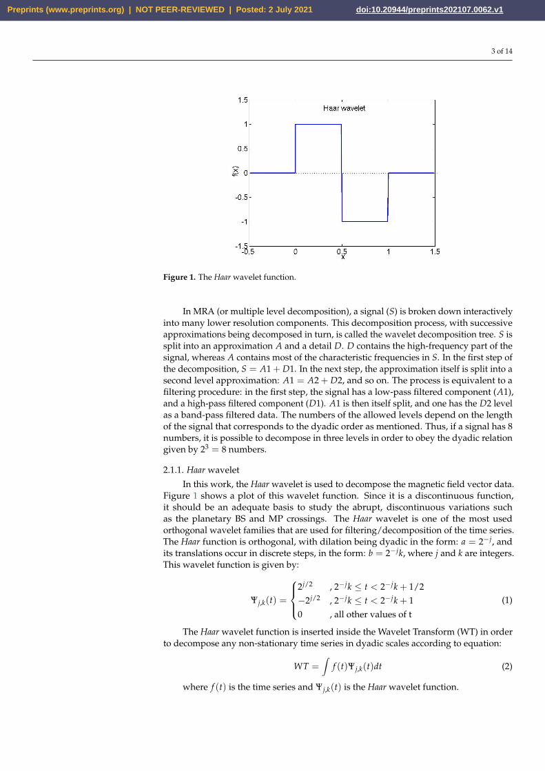
Figure 1. The Haar wavelet function.
In MRA (or multiple level decomposition), a signal (S) is broken down interactively90
into many lower resolution components. This decomposition process, with successive91
approximations being decomposed in turn, is called the wavelet decomposition tree. S is92
split into an approximation A and a detail D. D contains the high-frequency part of the93
signal, whereas A contains most of the characteristic frequencies in S. In the first step of94
the decomposition, S = A1 + D1. In the next step, the approximation itself is split into a95
second level approximation: A1 = A2 + D2, and so on. The process is equivalent to a96
filtering procedure: in the first step, the signal has a low-pass filtered component (A1),97
and a high-pass filtered component (D1). A1 is then itself split, and one has the D2 level98
as a band-pass filtered data. The numbers of the allowed levels depend on the length99
of the signal that corresponds to the dyadic order as mentioned. Thus, if a signal has 8100
numbers, it is possible to decompose in three levels in order to obey the dyadic relation101
given by 23 = 8 numbers.102
2.1.1. Haar wavelet103
In this work, the Haar wavelet is used to decompose the magnetic field vector data.104
Figure 1 shows a plot of this wavelet function. Since it is a discontinuous function,105
it should be an adequate basis to study the abrupt, discontinuous variations such106
as the planetary BS and MP crossings. The Haar wavelet is one of the most used107
orthogonal wavelet families that are used for filtering/decomposition of the time series.108
The Haar function is orthogonal, with dilation being dyadic in the form: a = 2−j, and109
its translations occur in discrete steps, in the form: b = 2−jk, where j and k are integers.110
This wavelet function is given by:111
Ψj,k(t) =
2j/2 , 2−jk ≤ t < 2−jk + 1/2−2j/2 , 2−jk ≤ t < 2−jk + 10 , all other values of t
(1)
The Haar wavelet function is inserted inside the Wavelet Transform (WT) in order112
to decompose any non-stationary time series in dyadic scales according to equation:113
WT =∫
f (t)Ψj,k(t)dt (2)
where f (t) is the time series and Ψj,k(t) is the Haar wavelet function.114
Preprints (www.preprints.org) | NOT PEER-REVIEWED | Posted: 2 July 2021 doi:10.20944/preprints202107.0062.v1

Version July 1, 2021 submitted to Atmosphere 4 of 14
2.2. Magnetometer data115
The high-resolution (5 s) CASSINI fluxgate magnetometer data [24], and the MES-116
SENGER magnetometer data [25] explored in this work are obtained from NASA’s117
Planetary Data System (PDS, http://pds.jpl.nasa.gov/). This resolution was selected118
because it is high enough to investigate the BS and MP crossings. At the same time, these119
can eliminate the very high frequency noise/oscillations that can appear in the higher120
resolution data. The interplanetary magnetic field (IMF) measurements are performed121
in the radial tangential normal (RTN) coordinate system, where R is directed from the122
Sun to the spacecraft, T = Ω× R/|Ω× R|, where Ω is the solar rotation axis, and N123
completes the right-hand system.124
3. Results and Discussions125
3.1. Original data126
The CASSINI spacecraft reached the near-Saturn environment during the end127
of June 2004 and made its first crossing of the planetary orbit [24,26]. Saturn’s mag-128
netosphere is characterized by large variations in its BS and MP boundaries due the129
internal factors and the solar wind pressure [9]. According to Dougherty et al. [26],130
were measured a total of 17 bow shock and 7 magnetopause crossings on the inbound131
and outbound passages. But it is important to note that the bow shock crossings were132
identified by abrupt increases in the magnetic field magnitude where the solar wind133
was compressed and decelerated. So, identification of these physical boundaries in the134
automatically way is important to study and understand the internal factors like the135
planetary periodic oscillations.136
Figure 2 shows the magnetic field components measured by the CASSINI magne-137
tometer during its inbound trajectory between 27 and 29 June 2004. The BS and MP138
crossings are indicated by the red and green lines, respectively. The Saturn magne-139
tosphere size was observed to be highly variable during this period, with 7 BS and 3140
MP crossings [26,27]. The BS crossings can be identified by the abrupt jumps in the141
magnetic field magnitude B. The region downstream of the BS exhibits large fluctua-142
tions in magnetic field components, indicating the magnetosheath. The MP crossings143
are identified by an enhancement in B and by abrupt directional changes in the mag-144
netic field components. Most of the BSs crossed during this period was found to be of145
the quasi-perpendicular type [27]. The BS and MP subsolar distances were found be146
∼40–49 Saturn radii (Rs) and ∼30–34 Rs, respectively [26].147
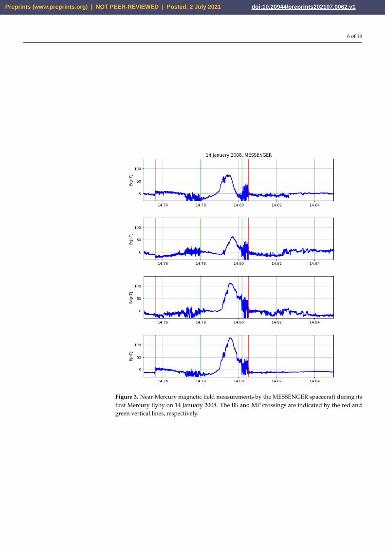
The MESSENGER spacecraft made the first of its three flybys of Mercury on 14148
January 2008 [20,28], and measured the near-Mercury magnetic field [25]. This is shown149
in Figure 3. MESSENGER, in its inbound trajectory, detected a BS, which was crossed at150
18:08:38 UT (inbound) and 19:18:55 UT (outbound) on 14 January. Before the inbound151
MP crossing at 18:43:02, the last extended interval of the southward magnetic field ended152
at 18:38:40. After MESSENGER exit the magnetosphere, the magnetic field was observed153
to be generally northward.154
3.2. Decomposed data155
The MESSENGER magnetic field magnitude B and vector components Br, Bt, Bn156
during the ∼1 h Mercury flyby were decomposed in orthonormal frequency levels using157
the Haar wavelet transform. The magnetic field data were decomposed in 14 scales158
according to data length used. We performed the variance by scale in order to identify159
the scale with the maximum energy. Figure 4 shows the variance by scale for the wavelet160
coefficients A and D (CAs and CDs) of B and components Br, Bt, Bn. It can be clearly161
seen that most of the energy for the wavelet coefficients (CAs and CDs) is concentrated162
at large scales, between the scales 11 and 14.163
As the maximum energy is found to be concentrated between the scales 11 and 14,164
CAs and CDs for the scales from 1 to 10 are assigned the value 0. This implies that the165
scales 1–10 do not contribute significantly to the total energy. However, the coefficients166
Preprints (www.preprints.org) | NOT PEER-REVIEWED | Posted: 2 July 2021 doi:10.20944/preprints202107.0062.v1

Version July 1, 2021 submitted to Atmosphere 5 of 14
Figure 2. Near-Saturn magnetic field measurements by the CASSINI spacecraft during its inboundtrajectory between 27 and 29 June 2004. The BS and MP crossings are indicated by the red andgreen vertical lines, respectively.
Preprints (www.preprints.org) | NOT PEER-REVIEWED | Posted: 2 July 2021 doi:10.20944/preprints202107.0062.v1
Version July 1, 2021 submitted to Atmosphere 6 of 14
Figure 3. Near-Mercury magnetic field measurements by the MESSENGER spacecraft during itsfirst Mercury flyby on 14 January 2008. The BS and MP crossings are indicated by the red andgreen vertical lines, respectively.
Preprints (www.preprints.org) | NOT PEER-REVIEWED | Posted: 2 July 2021 doi:10.20944/preprints202107.0062.v1

Version July 1, 2021 submitted to Atmosphere 7 of 14
Figure 4. Variance by scale for the magnetic field measurements by MESSENGER during itsMercury flyby shown in Figure 3. Left and right panels show the variances of CAs and CDs,respectively.
CAs and CDs were maintained from scale 11 onward. The magnetic field time series167
is reconstructed accordingly using the CAs and CDs for scales 11–14. Figure 5 shows168
the reconstructed magnetic field (in red) along with the original measurements (blue).169
The sharp changes in the magnetic field corresponding to the BS and MP crossings can170
be clearly identified in the reconstructed data using the coefficients CAs and CDs from171
scale 11 to 14.172
We applied the same procedure, as above, to the CASSINI magnetic field data173
(for Saturn encounter). Due the greater length of the CASSINI data (compared with174
MESSENGER data), we decomposed it in 15 scales. Figure 6 shows the variance by scale175
of the CAs and CDs coefficients (of the three magnetic field components and magnitude).176
The magnetic field variances increase from scale 11 and attain the maximum at scale177
15 for both wavelet coefficients. This implies that most of the energy is concentrated at178
large scales, from 11 to 15.179
Again, we used the same methodology (as applied to the MESSENGER data),180
by assigning zero to the CAs and CDs for scales 1–10, and those for scales 11–15 are181
maintained. The magnetic field time series is reconstructed accordingly using the CAs182
and CDs of scales 11–15. Figure 7 compares the original and reconstructed magnetic183
fields. Clearly, the magnetic field reconstructed using only scales 11 to 15 is able identify184
the majority of the sharp changes associated with BS and MP crossings.185
Figures 8 and 9 show the MRA decomposition levels only for the magnetic field186
magnitude B from CASSINI and MESSENGER, respectively. The same for magnetic187
field components is not shown for sake of brevity and to avoid repetition. The top188
panels correspond to the original data, followed by different decomposition levels in the189
lower panels and the reconstructed data in the bottom panels. A comparison between190
the top and bottom panels confirms the identical shape (variation) of the original and191
reconstructed data.192
Preprints (www.preprints.org) | NOT PEER-REVIEWED | Posted: 2 July 2021 doi:10.20944/preprints202107.0062.v1

Version July 1, 2021 submitted to Atmosphere 8 of 14
Figure 5. Comparison between the reconstructed magnetic field (red) with the MESSENGERmeasurements (blue) shown in Figure 3. The BS and MP crossings are indicated by the red andgreen vertical lines, respectively.
Figure 6. Variance by scale for the magnetic field measurements by CASSINI during its first Saturnflyby shown in Figure 2. Left and right panels show the variances of CAs and CDs, respectively.
Preprints (www.preprints.org) | NOT PEER-REVIEWED | Posted: 2 July 2021 doi:10.20944/preprints202107.0062.v1

Version July 1, 2021 submitted to Atmosphere 9 of 14
Figure 7. Comparison between the reconstructed magnetic field (red) with the CASSINI measure-ments (blue) shown in Figure 2. The BS and MP crossings are indicated by the red and greenvertical lines, respectively.
Preprints (www.preprints.org) | NOT PEER-REVIEWED | Posted: 2 July 2021 doi:10.20944/preprints202107.0062.v1

Version July 1, 2021 submitted to Atmosphere 10 of 14
Figure 8. The Haar wavelet decomposition levels for the CASSINI magnetic field magnitude. Toppanel shows the original measurement, followed by the MRA decomposition coefficients CA1to CA10 (left panels), and CD1 to CD10 (right panels), and the reconstructed data in the bottompanel.
Preprints (www.preprints.org) | NOT PEER-REVIEWED | Posted: 2 July 2021 doi:10.20944/preprints202107.0062.v1

Version July 1, 2021 submitted to Atmosphere 11 of 14
Figure 9. The Haar wavelet decomposition levels for the MESSENGER magnetic field magnitude.The panels are in the same format as in Figure 8.
Preprints (www.preprints.org) | NOT PEER-REVIEWED | Posted: 2 July 2021 doi:10.20944/preprints202107.0062.v1

Version July 1, 2021 submitted to Atmosphere 12 of 14
4. Discussion and Conclusions193
In this work we presented a wavelet technique to identify the abrupt changes in the194
magnetic field at the magnetospheric boundary crossings. The Haar wavelet was used195
to decompose the magnetic field data in different frequency levels. We analyzed the196
magnetic field measurements by CASSINI spacecraft during its Saturn orbit insertion,197
and by MESSENGER during its first Mercury flyby in 2008. The Haar wavelet multi-198
resolution analysis (MRA) was employed in this work to decompose the CASSINI and199
MESSENGER magnetometer data in orthonormal frequency levels. The objective was200
to identify the abrupt changes in the magnetic field when CASSINI and MESSENGER201
crossed the magnetospheric BS and MP of Saturn and Mercury, respectively. We have202
found that the Haar transform can be used to identify this type of abrupt boundaries.203
The methodology consisted in to perform the variance by scales in order to find204
out the scale where the energy is maximum. After that, the CAs and CDs from 1 to205
10 are assigned the value 0 for both spacecrafts. This implies that the scales 1–10 do206
not contribute significantly to the total energy. Results from the variance analysis by207
scale it was possible to note that the maximum energy were found different scales for208
each spacecraft, 10 up to 11 scales (1 3 h) for MESSENGER and the 15 scale ( 10 h) for209
CASSINI. Thus, although CASSINI and MESSENGER have shown maximum energy in210
different scales, but as the BS MPB are abrupt or quasi abrupt changes, the timescales to211
detect them are similar.212
The BS crossings have been identified from time-scales of ∼10–20 s to ∼10–40 min.213
However, time-scales of ∼10–40 min are more adequate to identify the BS crossings214
because much of the magnetic oscillations due to the magnetosheath waves are removed215
in these levels. On the other hand, multiple MP crossings are seen clearly only at ∼3–216
10 h time-scales. Further work should be conducted to use this technique to obtain217
quantitative information about the magnetospheric boundaries. This technique can218
be applied both to planetary boundaries as well as to detect discontinuities in the219
interplanetary space.220
Author Contributions: Conceptualization, M.J.A.B.; methodology, M.J.A.B.; validation, M.J.A.B.;221
formal analysis, M.J.A.B.; writing—original draft preparation, M.J.A.B.; writing—review and222
editing, E.E., A.M.S.F. and R.H.. All authors have read and agreed to the published version of the223
manuscript.224
Funding: MJAB was supported by CNPq agency contract number (PQ-302330/2015-1 and PQ-225
305692/2018-6) and FAPEG agency contract number 2012.1026.7000905. AMSF thanks to CNPq226
agency (project 301969/2021-3) for the support. EE would like to thank Brazilian agencies for227
research grants: CNPQ/PQ (302583/2015-7, 301883/2019-0) and FAPESP (2018/21657-1). The228
work of RH is funded by the Science and Engineering Research Board (SERB, grant no. SB/S2/RJN-229
080/2018), a statutory body of the Department of Science and Technology (DST), Government of230
India through Ramanujan Fellowship.231
Institutional Review Board Statement: Not applicable.232
Informed Consent Statement: Not applicable.233
Data Availability Statement: The CASSINI and MESSENGER magnetometer data are obtained234
from NASA’s Planetary Data System (PDS, http://pds.jpl.nasa.gov/).235
Conflicts of Interest: The authors declare no conflict of interest.236
Abbreviations237
The following abbreviations are used in this manuscript:238
239
Preprints (www.preprints.org) | NOT PEER-REVIEWED | Posted: 2 July 2021 doi:10.20944/preprints202107.0062.v1

Version July 1, 2021 submitted to Atmosphere 13 of 14
A ApproximationBS Bow shockCA Coefficient ACD Coefficient DD DetailIMF Interplanetary magnetic fieldMP MagnetopauseMRA Multi-resolution analysisPDS NASA’s Planetary Data SystemRme Mercury raiiRs Saturn radiiRTN Radial tangential normal coordinate systemS SignalUT Universal time
240
References241
1. Kivelson, M.G. Planetary magnetospheres. In Handbook of Space Environment 2007, 103, 469–242
492. doi:https://doi.org/10.1007/978-3-540-46315-3_19.243
2. Stern, D.P.; Ness, N.F. Planetary magnetospheres. Annual Reviews Astronomy and Astrophysics244
1982, 20, 139–161. doi:https://doi.org/10.1146/annurev.aa.20.090182.001035.245
3. Russell, C.T. The dynamics of planetary magnetospheres. Planetary and Space Science 2001,246
49, 1005–1030. doi:https://doi.org/10.1016/S0032-0633(01)00017-4.247
4. Kivelson, M.; Bagenal, F. Chapter 7. Planetary Magnetospheres. AAS/Division for Extreme248
Solar Systems Abstracts 2007, pp. 519–540. doi:10.1016/B978-012088589-3/50032-3.249
5. Slavin, J. Mercury’s magnetosphere. Advances in Space Research 2004, 33, 1859–1874. doi:250
10.1016/j.asr.2003.02.019.251
6. Slavin, J.; Baker, D.; Gershman, D.; Ho, G.; Imber, S.; Krimigis, S., Mercury’s Dynamic252
Magnetosphere; 2020; p. 461–496.253
7. André, N.; Dougherty, M.K.; Russell, C.T.; Leisner, J.S.; Khurana, K.K. Dynamics of the254
Saturnian inner magnetosphere: First inferences from the Cassini magnetometers about255
small-scale plasma transport in the magnetosphere. Geophysical Research Letters 2005,256
32, [https://agupubs.onlinelibrary.wiley.com/doi/pdf/10.1029/2005GL022643]. doi:257
https://doi.org/10.1029/2005GL022643.258
8. Southwood, D.J.; Chané, E. High-latitude circulation in giant planet magnetospheres. Journal259
of Geophysical Research: Space Physics 2016, 121, 5394–5403, [https://agupubs.onlinelibrary.wiley.com/doi/pdf/10.1002/2015JA022310].260
doi:https://doi.org/10.1002/2015JA022310.261
9. Jackman, C.M.; Thomsen, M.F.; Dougherty, M.K. Survey of Saturn’s Magnetopause and262
Bow Shock Positions Over the Entire Cassini Mission: Boundary Statistical Properties and263
Exploration of Associated Upstream Conditions. Journal of Geophysical Research – Space264
Physics 2019, 124, 85–89. doi:https://doi.org/10.1029/2019JA026628.265
10. Waite, J.H.; Combi, M.R.; Ip, W.H.; Cravens, T.E.; McNutt, R.L.; Kasprzak, W.; Yelle, R.;266
Luhmann, J.; Niemann, H.; Gell, D.; Magee, B.; Fletcher, G.; Lunine, J.; Tseng, W.L. Cassini267
Ion and Neutral Mass Spectrometer: Enceladus Plume Composition and Structure. Science268
2006, 311, 1419–1422, [https://science.sciencemag.org/content/311/5766/1419.full.pdf].269
doi:10.1126/science.1121290.270
11. Bolzan, M.J.A.; Franco, A.M.S.; Echer, E. A wavelet based method to remove the long term271
periodicities of geophysical time series. Advances in Space Research 2020, 66, 299–306. doi:272
https://doi.org/10.1016/j.asr.2020.04.014.273
12. Bolzan, M.J.A.; Guarnieri, F.L.; Vieira, P.C. Comparisons between two wavelet functions in274
extracting coherent structures from solar wind time series. Brazilian Journal of Physics 2009,275
39, 12–17. doi:https://doi.org/10.1590/S0103-97332009000100002.276
13. Kumar.; Foufoula-Georgiou. Wavelet analysis for geophysical applications. Reviews of277
Geophysics 1997, 35, 385–412. doi:https://doi.org/.278
14. Torrence, C.; Compo, G.P. A Practical Guide to Wavelet Analysis. Bulletin of the279
American Meteorological Society 1998, 79, 61–78. doi:https://doi.org/10.1175/1520-280
0477(1998)079<0061:APGTWA>2.0.CO;2.281
15. Gedalin, M.; Newbury, J.A.; Russell, C.T. Shock profile analysis using wavelet transform.282
Journal of Geophysical Research 1998, 103, 6503–6511. doi:https://doi.org/.283
Preprints (www.preprints.org) | NOT PEER-REVIEWED | Posted: 2 July 2021 doi:10.20944/preprints202107.0062.v1

Version July 1, 2021 submitted to Atmosphere 14 of 14
16. Tarasov, V.; Dubinin, E.; Perraut, S.; Roux, A.; Sauer, K.; Skalsky, A.; Delva, M. Wavelet284
application to the magnetic field turbulence in the upstream region of the Martian bow shock.285
Earth, Planets and Space 1998, 50, 699–708. doi:https://doi.org/10.1186/BF03352163.286
17. Espley, J.R.; Cloutier, P.A.; Brain, D.A.; Crider, D.H.; Acuna, M.H. Observations of low-287
frequency magnetic oscillations in the margina magnetosheath, magnetic pileup region and288
tail. Journal of Geophysical Research 2004, 109. doi:https://doi.org/10.1029/2003JA010193.289
18. Bolzan, M.J.A.; Sahai, Y.; Fagundes, P.R.; Rosa, R.R.; Ramos, F.M.; Abalde, J.R. Intermittency290
analysis of geomagnetic storm time-series observed in Brazil. Journal of Atmospheric and291
Solar-Terrestrial Physics 2005, 67, 1365–1372. doi:https://doi.org/10.1016/j.jastp.2005.06.008.292
19. Echer, E. Foreshock and magnetosheath waves at Uranus and Neptune studied with wavelet293
analysis. Advances in Space Research 2009, 44, 1030––1037. doi:https://doi.org/10.1016/j.asr.2009.05.024.294
20. Echer, E. Wavelet analysis of ULF waves in the Mercury’s magnetosphere. Revista Brasileira295
de Geofísica 2010, 28, 175–182. doi:https://doi.org/10.1590/S0102-261X2010000200003.296
21. Franco, A.M.S.; Franz, M.; Echer, E.; Bolzan, M.J.A. Wavelet analysis of low frequency plasma297
oscillations in the magnetosheath of Mars. Advances in Space Research 2020, 65, 2090–2098.298
doi:https://doi.org/10.1016/j.asr.2019.09.009.299
22. Echer, E. Multi-resolution analysis of global total ozone column during 1979-1992 Nimbus-7300
TOMS period. Annales Geophysicae 2004, 22, 1487–1493. doi:https://doi.org/10.5194/angeo-301
22-1487-2004.302
23. Percival, D.B.; Walden, A.T. Wavelet Methods for Time Series Analysis; Cambridge University303
Press, 2000.304
24. Dougherty, M.K.; Kellock, S.; Southwood, D.J.; Balogh, A.; Smith, E.J.; Tsurutani, B.T.;305
Gerlach, B.; Glassmeier, K.H.; Gleim, F.; Russell, C.T.; Erdos, G.; Neubauer, F.M.; Cowley,306
S.W.H. The Cassini magnetic field investigation. Space Science Reviews 2004, 114, 331–338.307
doi:https://doi.org/10.1007/s11214-004-1432-2.308
25. Anderson, B.J.; Acuña, M.H.; Lohr, D.A.; Scheifele, J.; Raval, A.; Korth, H.; Slavin, J.A. The309
Magnetometer Instrument on MESSENGER. Space Science Reviews 2007, 131, 417––450. doi:310
https://doi.org/10.1007/s11214-007-9246-7.311
26. Dougherty, M. K. Achilleos, N.; Andre, N.; Arridge, C.S.; Balogh, A.; Bertucci, C.; Burton,312
M.E.; Cowley, S.W.H.; Erdos, G.; Giampieri, G.; Glassmeier, K.H.; Khurana, K.K.; Leisner,313
J.; Neubauer, F.M.; Russell, C.T.; Smith, E.J.; Southwood, D.J.; Tsurutani, B.T. Cassini314
magnetometer observations during Saturn orbit insertion. Science 2005, 307, 1266–1270. doi:315
https://doi.org/10.1126/science.1106098.316
27. Achilleos, N.e.a. Orientation, location and velocity of Saturn’s bow shock: Initial re-317
sults from the Cassini spacecraft. Journal of Geophysical Research 2006, 111, xx–xx. doi:318
https://doi.org/10.1029/2005JA011297.319
28. Slavin, J.A.; Acuña, M.H.; Anderson, B.J.; Baker, D.N.; Benna, M.; Gloeckler, G.; Gold,320
R.E.; Ho, G.C.; Killen, R.M.; Korth, H.; Krimigis, S.M.; McNutt Jr., R.L.; Nittler, L.R.;321
Raines, J.M.; Schriver, D.; Solomon, S.C.; Starr, R.D.; Trávnícek, P.; Zurbuchen, T.H. Mer-322
cury’s magnetosphere after MESSENGER’s first flyby. Science 2008, 321, 85–89. doi:323
https://doi.org/10.1126/science.1159040.324
Preprints (www.preprints.org) | NOT PEER-REVIEWED | Posted: 2 July 2021 doi:10.20944/preprints202107.0062.v1