Identification of the Mechanical Subsystem of the NEES-UCSD

Identification of the Mechanical Subsystem of theNEES-UCSD Shake Table by a Least-Squares Approach

O. Ozcelik1; J. E. Luco2; and J. P. Conte3

Abstract: A least-squares method is used to determine the fundamental parameters of a simple mathematical model for the mechanicalsubsystem of the NEES-UCSD large high performance outdoor shaking table. The parameters identified include the effective horizontalmass, the effective horizontal stiffness, and the coefficient of the classical Coulomb friction and viscous damping elements representingthe various dissipative forces in the system. The values obtained for these parameters are validated by comparisons with previous resultsbased on an alternative identification method applicable only to periodic tests and by comparisons with experimental data obtained duringearthquake simulation tests and harmonic steady-state tests. The proposed identification approach works well for periodic sinusoidal andtriangular tests, earthquake simulation tests, and white noise tests with table root mean square above 10% of gravity.

DOI: 10.1061/�ASCE�0733-9399�2008�134:1�23�

CE Database subject headings: Shake table tests; Least squares method; Earthquakes; Simulation.

Introduction

Objectives of the Study

The new UCSD-NEES large high performance outdoor shakingtable �LHPOST� located at the Englekirk Structural EngineeringCenter at Camp Elliot Field Station, a site 15 km away from themain UCSD campus, is a unique facility that enables next gen-eration seismic experiments to be conducted on very large struc-tural and soil-foundation-structure-interaction systems. Largetests of a 21 m tall wind turbine, and a tall seven story, reinforcedconcrete shear wall building model �Fig. 1� have been conductedon the table. Optimization of the shake table performance duringthe tests, as well as the optimization of the experiments them-selves, including sensor location and safety precautions, requiresthe use of a detailed and reliable mathematical model of thecomplete facility. In general, a complete model of a shake tablesystem needs to include the mechanical, hydraulic, and electronicsubsystems. Typically, the steel platen, vertical and lateral bear-ings, hold-down struts, and actuators are included in the me-chanical subsystem; pumps, accumulator bank, line accumulators,servovalves, and surge tank are part of the hydraulic subsystem;and finally, controller, signal conditioners, sensors, and built-inanalog filters are included in the electronic subsystem.

In a previous paper �Ozcelik et al. 2007�, the authors devel-

1Dept. of Structural Engineering, Univ. of California, San Diego, 9500Gilman Dr., La Jolla, CA 92093-0085.



Note. Associate Editor: Lambros S. Katafygiotis. Discussion openuntil June 1, 2008. Separate discussions must be submitted for individualpapers. To extend the closing date by one month, a written request mustbe filed with the ASCE Managing Editor. The manuscript for this paperwas submitted for review and possible publication on February 9, 2007;approved on May 30, 2007. This paper is part of the Journal of Engi-neering Mechanics, Vol. 134, No. 1, January 1, 2008. ©ASCE, ISSN
0733-9399/2008/1-23–34/$25.00.
JOUR

oped a simplified analytical model for the mechanical subsystemof the UCSD-NEES shaking table, identified the parameters ofthe model using the data collected during the extensive shakedown tests of the table, and validated the model by detailed com-parisons with experimental data. The model and parameter iden-tification approach used in the previous study were based onanalysis of the hysteresis loops relating the feedback total actuatorforce to the feedback displacement, velocity, and acceleration ofthe platen recorded during periodic tests �both triangular and har-monic�. The procedure took advantage of the periodicity of themotion of the table during sinusoidal or triangular tests, to isolatethe inertial, elastic, and dissipative forces and their respectivedependence on acceleration, displacement, and velocity. The ap-proach is restricted to periodic tests, but does not assume a prioria linear model. Since the table motion for most future pretestswill consist of scaled down seismic motions or random whitenoise acceleration signals, it is necessary to develop and test iden-tification methods that do not depend on the periodicity of theexcitation.

The first objective of this study is to test the applicability of aparameter identification approach based on the standard least-squares method for shake table tests with very different excita-tions including periodic tests, white noise tests, and seismic tests.Of primary interest is the robustness of the parameter estimatesacross different types of tests. A second objective is to comparethe results of the least-squares identification approach with thoseobtained by consideration of the hysteresis loops for periodictests. A third objective of the study is to further validate the modeland identify parameters by detailed comparisons with experimen-tal data from different types of tests. Finally, the steady-statefrequency response of the shake table mechanical subsystem tocommanded harmonic displacement of the shake table is exam-ined. This analysis provides an additional verification of thenonlinear damping model used in the study, and illustrates theresponse of the table in the vicinity of the characteristic frequencyof the mechanical subsystem. It is envisioned that the analytical
model of the mechanical subsystem obtained in this and the pre-
NAL OF ENGINEERING MECHANICS © ASCE / JANUARY 2008 / 23

vious paper �Ozcelik et al. 2007� will be used in future studies tomodel the entire shake table system including all subsystemsmentioned previously.

It is expected that the present study will add to the growingliterature on the modeling of shake table systems �Hwang et al.1987; Rinawi and Clough 1991; Clark 1992; Conte and Trombetti2000; Williams et al. 2001; Shortreed et al. 2001; Crewe andSevern 2001; Trombetti and Conte 2002; Twitchell and Symans2003; Thoen and Laplace 2004�.

Overview of the UCSD-NEES Shake Table

The LHPOST consists of a moving steel platen �7.6 m wide by12.2 m long�; a reinforced concrete reaction block; two servo-controlled dynamic actuators with a force capacity in tension/compression of 2.6 and 4.2 MN, respectively; a platen sliding

Fig. 1. Seven-story full-scale R/C building slice, 19.2 m high

Table 1. Characteristics of the Triangular and Sinusoidal Tests Performe

TestsDisplacement

�cm�Velocity�cm/s�

Frequency�Hz� Tes

T1 5.00 1.00 0.05 S1

T2 7.50 1.50 0.05 S2

T3 12.50 2.50 0.05 S3

T4 50.00 10.00 0.05 S4

T5 25.00 10.00 0.10 S5

T6 62.50 25.00 0.10 S6

T7 37.50 25.00 0.167 S7

T8 75.00 50.00 0.167 S8

T9 46.88 75.00 0.40 S9

T10 62.50 100.00 0.40 S1

T11 75.00 150.00 0.50 S1

T12 67.50 180.00 0.667 S1

24 / JOURNAL OF ENGINEERING MECHANICS © ASCE / JANUARY 2008

system �six pressure balanced vertical bearings with a force ca-pacity of 9.4 MN each and a stroke of ±0.013 m�; an overturningmoment restraint system �a prestressing system consisting oftwo nitrogen-filled hold-down struts with a stroke of 2 m and ahold-down force capacity of 3.1 MN each�; a yaw restraint sys-tem �two pairs of slaved pressure balanced bearings along thelength of the platen�; a real-time multivariable controller; and ahydraulic power supply system. The technical specifications ofthe LHPOST include a stroke of ±0.75 m, a peak horizontal ve-locity of 1.8 m/s, a peak horizontal acceleration of 4.2 g for baretable conditions and 1.0 g for a rigid payload of 3.92 MN, a hori-zontal force capacity of 6.8 MN, an overturning moment capacityof 50 MN m, and a vertical payload capacity of 20 MN. Thefrequency bandwidth is 0–20 Hz. Other detailed specifications ofthe NEES-UCSD LHPOST can be found elsewhere �Van DenEinde et al. 2004�.

Experimental Data

The experimental data used to model and identify the fundamen-tal characteristics of the UCSD-NEES shake table were recordedduring shake-down tests, which were performed in the periodJune–September, 2004 to verify that the performance of the shaketable complies with the design specifications.

The tests designed for system characterization and identifica-tion purposes include periodic, earthquake, and white noise tests.For the periodic tests, sinusoidal �S� and triangular �T� waveformswere used with amplitude and frequency characteristics carefullyselected so as to span the entire operational frequency range ofthe system. For the earthquake tests, full and scaled versions ofhistoric earthquake records with different characteristics wereused. Finally, several white noise tests with different root meansquare table accelerations were performed on the system. All ofthese tests were incorporated in the identification process to makesure that the identified fundamental characteristics of the systemdo not change across test types and test characteristics. The de-tails of the tests performed on the system are summarized inTables 1 and 2.

Triangular and sinusoidal tests were performed withzero, 1,042.4 kN �6.9 MPa nitrogen pressure�, and 2,084.8 kN�13.8 MPa nitrogen pressure� forces in each of the two hold-downstruts in order to determine the effective horizontal stiffness pro-duced by the hold-down struts, and also to investigate the effectof vertical forces on the dissipative �friction, damping� forces. All

e System

Displacement�cm�

Velocity�cm/s�

Acceleration�g�

Frequency�Hz�

4.00 1.00 0.0003 0.04

4.00 1.51 0.0006 0.06

4.00 2.51 0.0016 0.10

4.00 10.05 0.0257 0.40

4.00 25.12 0.1608 1.00

10.00 25.12 0.0643 0.40

10.00 50.24 0.2573 0.80

10.00 75.36 0.5789 1.20

20.00 75.36 0.2895 0.60

20.00 100.48 0.5146 0.80

20.00 150.72 1.1578 1.20

20.00 179.61 1.6442 1.43

d on th

ts

0

1

2

triangular waves were rounded at their peak displacement values�at the change of velocity� with a phase of duration equal toone-tenth of the wave period and constant acceleration not ex-ceeding 2 g. All earthquake and white noise tests were performedwith a force of 2,084.8 kN �13.8 MPa nitrogen pressure� in eachof the two hold-down struts. All triangular, sinusoidal, earth-quake, and white noise tests were conducted several times inorder to check for repeatability of the results.

The total actuator force recorded during the last two sine andtriangular tests, namely S11, S12, T11, and T12, which had amaximum velocity near the velocity capacity of the table, weredistorted to such an extent that they could not be used for thepurpose of parameter identification. For this reason, these fourtests were not considered in all facets of this study.

Sensors and Data Acquisition System

Data were acquired by the built-in sensors and data acquisition�DAQ� system used for controlling the shaking table. The sam-pling frequency of the DAQ system is set at the default rate of1,024 Hz. This DAQ system also has low-pass antialiasing filter-ing capabilities. The displacement of the platen relative to thereaction block was measured by two digital displacement trans-ducers �Temposonics linear transducers� located on the east andwest actuators. The platen acceleration response was measured bytwo Setra-Model 141A accelerometers with a range of ±8 g and aflat frequency response from DC to 300 Hz. It should be notedhere that the signal conditioners used for the accelerometers in-clude a built-in analog low-pass filter with cutoff frequency set at100 Hz, implying that acceleration records have frequency con-tent only up to 100 Hz. Pressure in the various actuator chamberswas measured by four Precise Sensors-Model 782 pressure trans-ducers �located in the tension and compression chambers of eachactuator� with a pressure range from 0 to 68.9 MPa and a �sensor/DAQ� resolution of 689.5 Pa. These pressure transducers are lo-cated near the end caps of each actuator. Measured pressures areconverted to actuator forces by multiplying them with the corre-sponding actuator piston areas and combining the contributionsfrom both chambers. At this point, it is important to mention thatpressure recordings were high-pass filtered to remove their staticpressure components, but were not low-pass filtered. The velocityof the platen is the only response quantity measured indirectly. Toobtain a wideband estimate of velocity, the differentiated dis-placement sensor signal is combined with the integrated accelera-tion sensor signal via a crossover filter. This filter ensures that thevelocity estimate of the platen consists primarily of differentiated

Table 2. Characteristics of Earthquake and White Noise Tests Performedon the System

TestsPGA�g�

rms amplitude�g�

Scaling�%�

El Centro—1 0.07 — 20

El Centro—2 0.37 — 100

El Centro—3 1.11 — 300

Northridge 1.84 — 100

WN3%g 0.12 0.03 100

WN5%g 0.22 0.05 100

WN7%g 0.32 0.07 100

WN10%g 0.45 0.10 100

WN13%g 0.49 0.13 100

displacement at low-to-medium frequencies for which the dis-

JOUR

placement sensor is more accurate, and integrated acceleration atmedium-to-high frequencies for which the acceleration sensor ismore accurate �Thoen 2004�.

The MTS 469D Seismic Controller Recorder software wasused to record the digitized data; this software is an integral partof the MTS 469D Digital Controller. The sampling rate of thissoftware can be set at a different rate than the one used by thecontroller �1,024 Hz�. The sampling rate of the recorder was setat 512 Hz during the tests. Again, to prevent aliasing, the antialiasing digital filter built in the recorder was enabled during thetests. The sampling rate used on the recorder was sufficiently highfor all the tests performed on the system.

To interpret the results presented in the following sections, twoimportant general observations about the recorded data need to bepointed out here. In all the tests performed, two harmonic signalsat 10.66 Hz and 246 Hz were observed repeatedly, mainly in thetotal force and table acceleration records. The signal at 10.66 Hzcorresponds to the oil column frequency of the system. The ef-fective table mass of the system and the oil column within theactuators give rise to a mass-spring system with a natural fre-quency referred to as the oil column frequency �Thoen andLaplace 2004; Conte and Trombetti 2000; Kusner et al. 1992�.This oil column resonance frequency tends to be excited whenthere is a sudden change in the motion of the platen such as adirection reversal. The most likely source of the second harmonicsignal at 246 Hz is the resonance between the pilot stage and thethird stage of the servovalves. Due to low-pass filtering of theacceleration records at 100 Hz, this 246 Hz harmonic signal canbe observed only slightly in the acceleration records, but it isclearly observed in the actuator force records that are only sub-jected to high-pass filtering. The discrepancy between the filteringof the actuator force and platen acceleration data does not allowto simulate the high frequency harmonic components of the totalactuator force by use of the recorded table motion.

Model and Parameter Estimation by Least-SquaresApproach

Conceptual Model

A detailed analysis of the dynamics of the platen and hold-downstruts �Ozcelik et al. 2007� indicates that several nonlinear termsaffecting the inertial and elastic forces are small and can be ne-glected. Under these conditions, a simplified mathematical modelof the shake table system with a relatively small number of un-known parameters can be formulated. This model is representedin Fig. 2, where Fact�t�=total effective actuator force applied on

Fig. 2. Conceptual mechanical model of the table with modelparameters Me, Ke, Ce, and F�e

to be identified through periodic,earthquake, and white noise tests

the pistons of the two horizontal actuators; Me=effective mass


of the platen �including the mass of the moving parts of the hori-zontal actuators and a portion of the mass of the hold-downstruts�; Ke=total effective horizontal stiffness provided by thetwo hold down struts; Ce=effective viscous damping coefficient;F�e

=effective Coulomb friction force due to various sources;and ux�t�=total horizontal displacement of the platen along thelongitudinal direction.

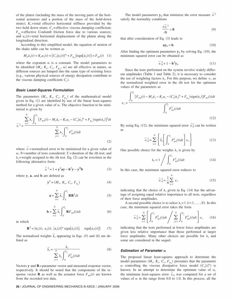
According to this simplified model, the equation of motion ofthe shake table can be written as

Meux�t� + Keux�t� + �Ce�ux�t�� + F�e�sign�ux�t�� = Fact�t� �1�

where the exponent � is a constant. The model parameters tobe identified �Me, Ke, Ce, F�e

, �� are all effective in nature, asdifferent sources are lumped into the same type of resisting force�e.g., various physical sources of energy dissipation contribute tothe viscous damping coefficient Ce�.

Basic Least-Squares Formulation

The parameters �Me, Ke, Ce, F�e� of the mathematical model

given in Eq. �1� are identified by use of the linear least-squaresmethod for a given value of �. The objective function to be mini-mized is given by

�2 =

�i=1

N

�i�0

Ti

�Fact�t� − Meux − Keux − �Ce�ux�� + F�e�sign�ux��2dt

�j=1

N

� j�0

Tj

Fact2 �t�dt

�2�

where �=normalized error to be minimized for a given value of�; N=number of tests considered; Ti=duration of the ith test; and�i=weight assigned to the ith test. Eq. �2� can be rewritten in thefollowing alternative form:

�2 = 1 + yTay − bTy − yTb �3�

where y, a, and b are defined as

yT = �Me, Ke, Ce, F�e� �4�

a = �i=1

N

�i�0

Ti

RRTdt �5�

b = �i=1

N

�i�0

Ti

RFact�t�dt �6�

in which

RT = �ux�t�, ux�t�, �ux�t�� sign�ux�t��, sign�ux�t�� 7�

The normalized weights �i appearing in Eqs. �5� and �6� are de-fined as

�i =�i

�j=1

N

� j�0

Tj

Fact2 �t�dt

�8�

Vectors y and R=parameter vector and measured response vector,respectively. It should be noted that the components of the re-sponse vector R as well as the actuator force Fact�t� are known
from the recorded test data.

The model parameters y0 that minimize the error measure �2

satisfy the normality conditions

��2

�y= 0 �9�

that after consideration of Eq. �3� leads to

ay0 = b �10�

After finding the optimum parameters y0 by solving Eq. �10�, theminimum squared error can be obtained as

�02 = 1 − bTy0 �11�

Since the tests performed on the system involve widely differ-ent amplitudes �Table 1 and Table 2�, it is necessary to considerthe use of weighting factors �i. For this purpose, we define �i asthe normalized weighted error in the ith test for the optimumvalues of the parameters as

�i =

�0

Ti

�Fact�t� − Meux − Keux − �Ce�ux�� + F�e�sign�ux��Fact�t�dt

�0

Ti

Fact2 �t�dt

�12�

By using Eq. �12�, the minimum squared error �02 can be written

as

�02 = �

i=1

N �i��0

Ti

Fact2 �t�dt��i �13�

One possible choice for the weights �i is given by

�i = 1��0

Ti

Fact2 �t�dt �14�

In this case, the minimum squared error reduces to

�02 =

1

N�i=1

N

�i �15�

indicating that the choice of �i given in Eq. �14� has the advan-tage of assigning equal relative importance to all tests, regardlessof their force amplitudes.

A second possible choice is to select �i=1 �i=1, . . . ,N�. In thiscase, the minimum squared error takes the form

�02 = �

i=1

N ��0

Ti

Fact2 �t�dt��

j=1

N �0

Tj

Fact2 �t�dt��i �16�

indicating that the tests performed at lower force amplitudes aregiven less relative importance than those performed at largerforce amplitudes. Many other choices are possible for �i andsome are considered in the sequel.

Estimation of Parameter �

The proposed linear least-squares approach to determine themodel parameters �Me, Ke, Ce, F�e

� presumes that the parameter� controlling the viscous dissipative force model �Ce�x�� isknown. In an attempt to determine the optimum value of �,the minimum least-squares error �0 was computed for a set of
values of � in the range from 0.0 to 1.0. In this process, all the

triangular tests for a nitrogen pressure of 13.8 MPa in the hold-down struts were considered with four choices for the weights �i,namely, �i

�1�=1, �i�2�=1/�0

Ti�ux�2dt, �i�3�=1/ ��0

Ti�ux�2dt�1/2, and�i

�4�=1/�0TiFact

2 �t�dt were used.

The results obtained for �0 as a function of � and the types of

weights �i are presented in Fig. 3, which shows that �0 is rela-tively independent of the types of weights �i and of the value ofparameter �. These results indicate that the overall minimumleast-squares error combining several tests may not be the bestcriterion to determine the optimum value of the parameter �.Instead, the stability of the parameters Ce and F�e

identified fromindividual tests at different amplitudes is used to determine theoptimum value of parameter �. Thus, the least-squares identifica-tion procedure was applied separately to the data from each of thesinusoidal Tests S1 through S10 of increasing peak velocity forseveral values of parameter �. The resulting estimates of F�e

andCe for �=1 and �=1/2 are presented in Fig. 4. In the case of alinear viscous force model ��=1�, the estimate of the Coulombfriction force F�e

is relatively constant from test to test �Fig. 4�a��,but the viscous coefficient Ce decreases with test order and veloc-ity �Fig. 4�c��. This result indicates that the dissipative forcesduring sinusoidal tests cannot be represented by a simple combi-nation of Coulomb friction and linear viscous damping. The re-sults for a nonlinear viscous force ��=1/2� show a more constantestimate for Ce �Fig. 4�d��, but the estimated friction force F�echanges somewhat from test to test in this case �Fig. 4�b��. At-tempts with other values of � do not lead to results significantlymore uniform than those obtained for �=1/2. Thus, the value�=1/2 was adopted in this study.

Figs. 4�e and f� show the estimated total dissipative force atthe maximum achieved velocity for each test plotted versus thepeak velocity. The total dissipative force is calculated as

Fd = �Ce�ux�� + F�e�sign�ux� �17�

where F�eand Ce=parameter values estimated by the least-

squares approach for each particular test. Comparison of the re-sults in Figs. 4�e and f� indicate that two significantly differentmodels ��=0.5 and �=1.0� lead to essentially the same total dis-sipative force. Thus, it appears that individual test data may notbe sufficient to discriminate between the different combinations

Fig. 3. Minimum least-squares error �0 as a function of parameter �and for different types of weights �i �i=1¯12�

of �, F�e, and Ce �i.e., eliminate compensation effects�.

JOUR

Equivalent Linear Viscous Damper

To understand the tradeoffs between the Coulomb friction forceF�e

sign�ux� and the viscous damping force Ce�ux��sign�ux�, it isconvenient to introduce an equivalent linear viscous dampercharacterized by the damping coefficient Ce. This constant Ce isdefined such that the energy dissipated by the equivalent linearviscous damper over a cycle of periodic response of duration T isequal to that dissipated by the complete model in Eq. �17�. The

resulting expression for Ce is given by

Ce = �1F�e/� + �2Ce/�

1−� �18�

where � denotes the peak velocity, and

�1 = ��0

T

�ux�dt��0

T

u2xdt �19�

�2 = �1−��0

T

�ux�1+�dt��0

T

ux2dt �20�

In the particular case of a periodic triangular test with velocity

� and period T, it can be shown that �1=�2=1 and Ce=F�e/�

+Ce /�1−�. In the case of a sinusoidal test with velocityux�t�=� sin�2�t /T� characterized by the peak velocity � and pe-riod T, the factors �1 and �2 become

�1 = � 4

�� 21�

�2 =2�

��

1 + ��2��/2�

��22�

where ��·� denotes the gamma function. In particular, for the

special case �=1/2, then �1=1.273, �2=1.113, and Ce

=1.273F�e/�+1.113Ce /��.

Eq. �18� indicates that for a given value of the peak velocity �,different combinations of F�e

and Ce can lead to the same equiva-lent linear viscous damping coefficient and thus to the same totalenergy dissipation. Hence, to properly identify the Coulomb andviscous dissipative forces, it is necessary to consider simulta-neously several tests with very different velocities. The last termin Eq. �18� and the results in Fig. 4�c� for the estimated linearviscous damping coefficient ��=1� suggest that an effectiveviscous damper with a fractional power law is a more suitablerepresentation of the data.

In what follows, the data from different sets of tests will bepooled together, and the parameter � will be set to 0.5 on thebasis of the relative stability of the estimates of F�e

and Ce ob-tained from different tests. The resulting estimates of Me, Ke, andof the total dissipative force are relatively independent of theassumed value for the parameter �.

Parameter Estimation

The parameter identification was conducted separately for ninesets of pooled data. Three of the sets consist of the combination often sinusoidal tests for hold-down pressures of 0, 6.9, and13.8 MPa, respectively. A second group of three sets involve thecombination of ten triangular tests also for hold-down nitrogenpressures of 0, 6.9, and 13.8 MPa, respectively. The seventh set
corresponds to the three scaled El Centro seismic tests at the

operating hold-down nitrogen pressure of 13.8 MPa. The eighthset consists of data from three white noise tests with rms ampli-tudes of 0.03, 0.05, and 0.07 g, respectively, conducted at theoperating hold-down nitrogen pressure. Finally, the ninth set isdefined by two white noise tests with rms amplitudes of 0.10 and0.13 g, respectively, conducted at the operating hold-down nitro-gen pressure.

Effective Mass Estimation

The results of the least-squares identification for the effectivemass Me are presented in Table 3 for two choices of the weightscorresponding to �i=�i

�1� and �i=�i�2�. With one exception, the

estimated effective masses obtained from different test types,different nitrogen pressure conditions in the hold-down struts,and different weights are in good agreement. It appears that Me

increases slightly with the nitrogen pressure in the hold-downstruts, thus suggesting some correlation with the effective stiff-

Fig. 4. �a�, �b�: Coulomb friction forces; �c�, �d�: viscous dampingdifferent sine tests for �=1.0 and �=0.5

ness Ke. The average of the estimates of Me for the periodic tests


Table 3. Estimates of the Effective Mass of the System for Different TestTypes and Different Levels of Nitrogen Pressure in the Hold-Down Struts��=0.5�

Test type—nitrogen pressure

Me

�tons�

�i=�i�1�

i=1, . . . ,12�i=�i

�2�

i=1, . . . ,12

Sine—0.0 MPa 134.7 114.1

Triangular—0.0 MPa 138.4 139.0

Sine—6.9 MPa 143.2 143.5


Sine—13.8 MPa 143.9 144.5


El Centro tests—13.8 MPa 146.2 145.7

WN �0.03, 0.05, 0.07 g rms�—13.8 MPa 143.6 143.5

WN �0.10, 0.13 g rms�—13.8 MPa 144.0 144.0

coefficient; and �e�, �f�: total dissipative force estimated from each of ten

at the hold-down nitrogen operating pressure of 13.8 MPa is144 tons. The estimate of Me from the white noise tests at 0.10and 0.13 g rms acceleration is also 144 tons, matching the aver-age result for the triangular and sine tests. The average estimatesof the effective mass from the white noise tests with smaller am-plitudes �0.03–0.05–0.07 g rms acceleration� is 143.6 tons,which is also close to the average estimate from the periodic tests.The estimates of Me from higher frequency earthquake tests areon the average of 1.4% larger than those obtained from lowerfrequency triangular and sine tests.

The one deficient estimate of the effective system mass occursfor the sinusoidal tests at zero hold-down nitrogen pressure andfor the weights �i=�i

�2�. The problem is associated with the lowamplitudes, velocities, and accelerations achieved during Tests S1through S4. When these four tests are removed from the pool, theestimate of the effective mass increases from 114.1 to 146.9 tons.In addition, when all S1 through S10 tests are used but the vis-cous damping coefficient is constrained �as described later�, thenthe estimate of the effective mass is 146.1 tons.

Effective Horizontal Stiffness Estimation

The results obtained for the effective horizontal stiffness Ke arereported in Table 4. It should be noted here that for tests corre-sponding to zero nitrogen pressure in the hold-down struts, thereis no horizontal stiffness acting on the system.

The estimates of the effective stiffness Ke obtained from theperiodic tests increase linearly with the nitrogen pressure in the

Table 4. Estimates of the Effective Horizontal Stiffness of theHold-Down Struts for Different Test Types and Different Levels ofNitrogen Pressure in the Hold-Down Struts ��=0.5�

Test type—nitrogen pressure

Ke

�MN/m�

�i=�i�1�

i=1, . . . ,12�i=�i

�2�

i=1, . . . ,12

Sine—6.9 MPa 0.611 0.640


Sine—13.8 MPa 1.246 1.281



WN �0.03, 0.05, 0.07 g rms�—13.8 MPa 1.916 2.132

WN �0.10, 0.13 g rms�—13.8 MPa 1.392 1.417

Table 5. Estimates of Coulomb Friction Force and Viscous Damping Co

Tests types—nitrogen pressure

Uncon

F�e�kN�

��1� ��2�

Sine—0.0 MPa 17.4 16.6


Sine—6.9 MPa 26.1 26.8


Sine—13.8 MPa 30.1 30.6



WN �0.03, 0.05, 0.07 g rms�—13.8 MPa 14.14 14.6

WN �0.10, 0.13 g rms�—13.8 MPa 9.19 9.4

JOUR

hold-down struts from an average value of 0.635 MN/m for apressure of 6.9 MPa to an average value of 1.263 MN/m for apressure of 13.8 MPa. The triangular tests involve larger forces inthe hold-down struts and smaller inertia forces than the sinusoidaltests and appear to yield more stable estimates of Ke.

The average estimate of Ke obtained from the El Centro tests is1.238 MN/m, which is 2% lower than the corresponding averageestimate obtained from the periodic tests. The results in Tables 3and 4 indicate that for the earthquake tests there is some compen-sation effects between the estimates of Me and Ke, with Me being1.3% larger and Ke 2% lower than the corresponding estimatesfrom the periodic tests. The average estimate of Ke from the 0.10and 0.13 g rms acceleration white noise tests is 1.405 MN/m,which is 11.2% larger than the corresponding average estimatefrom the periodic tests. The estimates of Ke based on the low-amplitude �0.03, 0.05, and 0.07 g rms acceleration� white noisetests are significantly higher than the other estimates and appearto be in error. The low amplitude white noise tests involve ex-tremely small displacements, but significant accelerations. Underthese conditions, the elastic forces are much smaller than the in-ertia forces, and the stiffness cannot be determined accurately.

From the above results, it can be concluded that the effectivehorizontal stiffness of the system is approximately 1.263 MN/min the nominal case corresponding to a nitrogen pressure of13.8 MPa in the hold-down struts. For a nitrogen pressure of6.9 MPa, the effective stiffness is reduced to 0.63 MN/m.

Estimation of Dissipative Force

The estimates of the dissipative force parameters F�eand Ce

obtained from the nine pooled sets of data for �=0.5 and weight-ing factors ��i=�i

�1� and �i=�i�2�� are reported in Table 5 in the

columns labeled “unconstrained.” The results indicate that bothF�e

and Ce increase with the hold-down nitrogen pressure. Theaverage values of F�e

over the two weighting factors and the twotypes of tests �triangular and sinusoidal�, are 16.7, 25.9, and29.5 kN for the three hold-down nitrogen pressures �0.0, 6.9, and13.8 MPa�. The corresponding average values of Ce are 18.4,34.5, and 46.0 kN�s /m�0.5. Although the unconstrained estimatesof F�e

are fairly stable for a given hold-down nitrogen pressure,the corresponding unconstrained estimates of Ce vary signifi-cantly with weighting factor and test type.

A second set of estimates for F�ewas obtained by repeating

the least-squares based estimation process with Ce constrained to

nts Obtained by Least-Squares Approach with Pooled Datasets ��=0.5�

d Constrained

Ce

�kN �s /m�1/2�F�e�kN�

Ce

�kN �s /m�1/2��1� ��2� ��1� ��2� ��1� ��2�

1.4 17.6 12.4 5.7 45.9 45.9

3.1 21.5 8.7 5.9 45.9 45.9

1.1 36.1 23.8 19.8 45.9 45.9

1.2 29.4 20.7 24.2 45.9 45.9

9.4 48.4 27.5 23.9 45.9 45.9

2.3 43.8 25.9 28.6 45.9 45.9

1.3 62.1 26.4 30.2 45.9 45.9

0.03 149.8 25.8 26.3 45.9 45.9

0.21 123.1 24.3 24.4 45.9 45.9

efficie

straine

�

2

1

4

3

4

4

5

14

12


be equal to 46.0 �kN�s /m�0.5� corresponding to the average esti-mate of Ce over the sinusoidal and triangular tests for a hold-down nitrogen pressure of 13.8 MPa. The resulting constrainedestimates of F�e

are also given in Table 5. The constrained esti-mates of F�e

are more stable across test type and weighting fac-tor. The average constrained value of F�e

over the sinusoidaland triangular tests and the two weighting factors are 8.2, 22.1,and 26.5 kN for the hold-down nitrogen pressures of 0, 6.9, and13.8 MPa, respectively. The constrained estimates of the frictionforce F�e

from the scaled El Centro tests and from the two sets ofwhite noise tests are 28.3, 26.1, and 24.4 kN, respectively, whichare close to the average estimate of 26.5 from the periodic tests.The deviations from the average of the periodic tests are as highas 8%, but these differences amount to less than 2.1 kN, which iswell within the margin of error in estimating the dissipative forcesfrom the measured data.

Both the constrained and unconstrained estimates of F�esug-

gest that the friction forces depend on the hold-down nitrogenpressure and, consequently, are mostly associated with friction onthe vertical bearings of the platen. The unconstrained estimatesof the effective viscous damping coefficient Ce also depend onthe hold-down nitrogen pressure, suggesting that the dissipativeviscous forces are also related to the vertical bearings. Theconstrained estimate of Ce is selected to be independent of thehold-down nitrogen pressure and would be consistent with vis-cous forces in the lateral bearings of the platen and in the actua-tors, instead of the vertical bearings. Both sets of estimates of F�eand Ce lead to essentially the same total dissipative forces �withinthe margin of error� and, consequently, it is not possible todiscriminate between these two possibilities. The constrained es-timates will be used in the sequel.

The results given in Table 5 indicate that the constrained esti-mate of F�e

based on the scaled El Centro tests is within 7% ofthe average value of F�e

based on sinusoidal and triangular tests.The corresponding difference for white noise tests is less than8%. Thus, the constrained least-squares approach can identify the

Fig. 5. Average Coulomb friction forces ��1� and ��2�� as a functionof total vertical force on vertical bearings �dispersion bounds for sineand triangular tests�

total friction force from a variety of tests.


Decomposition of the Total Friction Force

The two major sources of Coulomb-type friction in the system arethe vertical and lateral bearings. The inferred values for the totalfriction force F�e

obtained from tests performed under differenthold-down nitrogen pressures can be used to quantify these twosources of friction. The average of the estimates of F�e

obtainedfrom sinusoidal and triangular tests for different levels of nitrogenpressure in the hold-down struts are shown in Fig. 5 versus thetotal corresponding vertical force acting on the vertical bearings.The total vertical force was obtained experimentally from read-ings of the pressures on the vertical bearings for the differenthold-down pressures. The forces correspond to 1.613, 3.698, and5.783 MN for hold-down nitrogen pressures of 0.0, 6.9, and13.8 MPa, respectively. A least-squares fit to the three points thusobtained leads to a line with a slope of 0.39% and an intercept of4.1 kN. It appears then that the total friction force F�e

can beexpressed as F�e

=F�,lat+�eFz, where Fz=total vertical force act-ing on the vertical bearings; F�,lat=4.1 kN=friction force exertedby the lateral bearings; and �e=0.39% =Coulomb friction coeffi-cient in the vertical bearings.

A decomposition of the dissipative forces into friction compo-nents on the horizontal and vertical bearings and viscous forces ispresented in Fig. 6, based on tests performed under the nominalhold-down nitrogen pressure of 13.8 MPa. Similar results werefound from triangular tests performed under the same hold-downnitrogen pressure.

The results in Fig. 6 indicate that for a table velocity of75 cm/s, for example, 6% of the total dissipative force is dueto Coulomb friction on the lateral bearings, 34% to Coulombfriction on the vertical bearings, and 60% to viscous dampingforces.

Fig. 6 also shows a comparison between the total dissipativeforce obtained by use of the overall inferred model representedby Eq. �1� �curve in Fig. 6� and the corresponding forces obtained

Fig. 6. Decomposition of the total dissipative force into its threemajor components

through �constrained� least-squares parameter estimation for

individual sinusoidal and triangular tests �symbols in Fig. 6�. Itis observed that the inferred model slightly underestimatesthe total dissipative force for sinusoidal tests, but overestimatesthe total dissipative force for triangular tests.

Comparison of Parameters Identified by Periodic,White Noise, and Earthquake Simulation Tests

Before comparing the parameter identification results obtained byapplying the least-squares method to different types of tests in-cluding periodic, white noise, and earthquake tests, a comparisonof the results obtained from two different identification methodsbased on periodic sinusoidal and triangular test data is presented.The values of the parameters identified in the present paper by the�constrained� least-squares approach are compared in Table 6 withthose obtained previously �Ozcelik et al. 2007� by analysis of theobserved hysteresis loops. The estimates of the effective mass Me

and effective stiffness Ke obtained using the two identificationmethods are in excellent agreement. The details of the parametersrelated to the dissipative forces are slightly different, but thevalues of the viscous damping coefficient Ce are within 3%. Inaddition, the total static Coulomb friction forces F�e

obtainedby the two methods differ by 2.7% corresponding to 0.7 kN,which is well below the margin of error. The results obtained bythe least-squares approach led to slightly larger dissipative forces�2.8% at a velocity of 1 m/s�, but the difference amounts to about2.0 kN for a velocity of 1 m/s.

Next, we examine the stability of the results of parameter iden-tification by the least-squares method when applied to differenttypes of tests including periodic, white noise, and earthquaketests. A summary of the results obtained is presented in Table 7.Comparison of the results indicates that for the scaled earthquaketests, the estimated mass is slightly larger �1.4%�, the estimatedstiffness slightly smaller �2.0%�, and the �constrained� friction

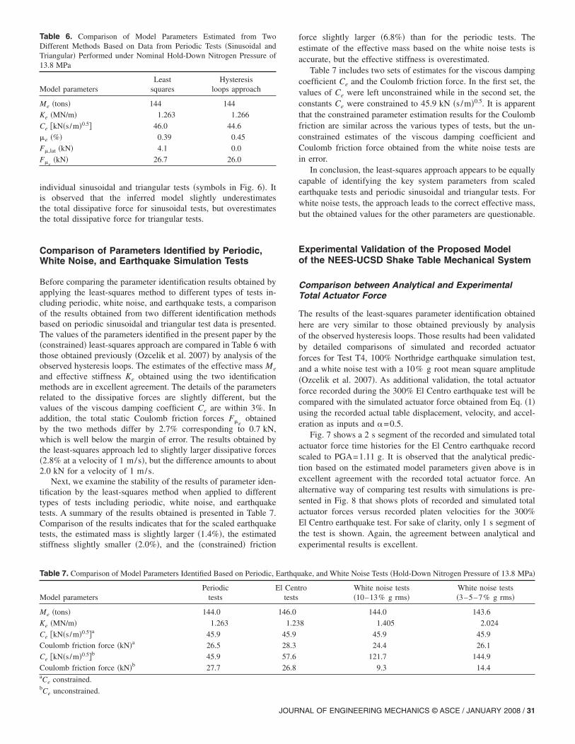
Table 6. Comparison of Model Parameters Estimated from TwoDifferent Methods Based on Data from Periodic Tests �Sinusoidal andTriangular� Performed under Nominal Hold-Down Nitrogen Pressure of13.8 MPa

Model parametersLeast

squaresHysteresis

loops approach

Me �tons� 144 144

Ke �MN/m� 1.263 1.266

Ce �kN�s /m�0.5� 46.0 44.6

�e �%� 0.39 0.45

F�,lat �kN� 4.1 0.0

F�e�kN� 26.7 26.0

Table 7. Comparison of Model Parameters Identified Based on Periodic, E

Model parametersPeriodic

testsE

Me �tons� 144.0

Ke �MN/m� 1.263

Ce �kN�s /m�0.5�a 45.9

Coulomb friction force �kN�a 26.5

Ce �kN�s /m�0.5�b 45.9

Coulomb friction force �kN�b 27.7aCe constrained.b
Ce unconstrained.
JOUR

force slightly larger �6.8%� than for the periodic tests. Theestimate of the effective mass based on the white noise tests isaccurate, but the effective stiffness is overestimated.

Table 7 includes two sets of estimates for the viscous dampingcoefficient Ce and the Coulomb friction force. In the first set, thevalues of Ce were left unconstrained while in the second set, theconstants Ce were constrained to 45.9 kN �s /m�0.5. It is apparentthat the constrained parameter estimation results for the Coulombfriction are similar across the various types of tests, but the un-constrained estimates of the viscous damping coefficient andCoulomb friction force obtained from the white noise tests arein error.

In conclusion, the least-squares approach appears to be equallycapable of identifying the key system parameters from scaledearthquake tests and periodic sinusoidal and triangular tests. Forwhite noise tests, the approach leads to the correct effective mass,but the obtained values for the other parameters are questionable.

Experimental Validation of the Proposed Modelof the NEES-UCSD Shake Table Mechanical System

Comparison between Analytical and ExperimentalTotal Actuator Force

The results of the least-squares parameter identification obtainedhere are very similar to those obtained previously by analysisof the observed hysteresis loops. Those results had been validatedby detailed comparisons of simulated and recorded actuatorforces for Test T4, 100% Northridge earthquake simulation test,and a white noise test with a 10% g root mean square amplitude�Ozcelik et al. 2007�. As additional validation, the total actuatorforce recorded during the 300% El Centro earthquake test will becompared with the simulated actuator force obtained from Eq. �1�using the recorded actual table displacement, velocity, and accel-eration as inputs and �=0.5.

Fig. 7 shows a 2 s segment of the recorded and simulated totalactuator force time histories for the El Centro earthquake recordscaled to PGA=1.11 g. It is observed that the analytical predic-tion based on the estimated model parameters given above is inexcellent agreement with the recorded total actuator force. Analternative way of comparing test results with simulations is pre-sented in Fig. 8 that shows plots of recorded and simulated totalactuator forces versus recorded platen velocities for the 300%El Centro earthquake test. For sake of clarity, only 1 s segment ofthe test is shown. Again, the agreement between analytical andexperimental results is excellent.

ake, and White Noise Tests �Hold-Down Nitrogen Pressure of 13.8 MPa�

ro White noise tests�10–13% g rms�

White noise tests�3–5–7% g rms�

144.0 143.6

8 1.405 2.024

45.9 45.9

24.4 26.1

121.7 144.9

9.3 14.4

arthqu

l Centtests

146.0

1.23

45.9

28.3

57.6

26.8


Comparison between Analytical and ExperimentalSteady-State Frequency Response

The mechanical system described by Eq. �1� has an undampednatural frequency given by �e=�Ke /Me corresponding to a fre-quency of 0.471 Hz �period of 2.12 s�. One way of testing theenergy dissipation model included in Eq. �1� is to consider thesteady-state response of the system to harmonic excitation withfrequencies in the vicinity of the system’s natural frequency �e. Inthe vicinity of �e, the inertial and elastic forces approximatelycancel each other, and the actuator force is approximately equal tothe damping force.

With the above objective in mind, the equation of motion ofthe system �Eq. �1�� was integrated numerically for a sinusoidalactuator force Fact�t�=F0 sin�2�ft�, and the peak amplitude umax

of the steady-state displacement was obtained for different valuesof the excitation frequency f and the force amplitude F0. Theo-retical dynamic amplification factors Rd=umax/ �F0 /Ke� for differ-ent values of F0 in the range from 49 to 250 kN were calculatedand are shown versus frequency f �in Hz� in Fig. 9 in the formof several frequency response curves. Shown also in Fig. 9 arethe values of the experimental ratios umax/ �Fmax/Ke� obtained

Fig. 7. Comparison of recorded and simulated total actuator forcesfor the 300% El Centro earthquake test �13.8 MPa nitrogen pressurein the hold-down struts�

Fig. 8. Recorded and simulated total actuator force versus recordedtable velocity plots for 300% El Centro earthquake test �13.8 MPapressure in the hold-down struts�


for several sinusoidal tests plotted versus the frequency of thetest. Since the system is nonlinear, these two ratios are not strictlycomparable. In the experimental ratio, umaxmaximum valueof the feedback table displacement �which may not be exactlysinusoidal� for a commanded sinusoidal displacement, andFmaxpeak value of the recorded total actuator force, which alsomay not be exactly sinusoidal. In the theoretical dynamic am-plification factor Rd, the actuator force is sinusoidal, but thecalculated displacement response is not exactly sinusoidal. Inspite of these differences, the theoretical dynamic amplificationfactors �curves in Fig. 9� and the experimental ratios �black dotsin Fig. 9� follow the same trends. The experimental ratios forTests S3, SR7, and SE4, all with frequencies below the frequencyof the system, fall on the left branches of the dynamic amplifica-tion curves. The measured peak actuator forces during these testswere 83, 262, and 384 kN, respectively, and the correspondingexperimental ratios fall close to the dynamic amplification curvesshown for 100.8 and 250 kN. The experimental ratios for TestsSE5, SR9, S9, S7, and S5, which have peak actuator forces in therange from 133 to 242 kN, fall between the descending branchesof the dynamic amplification curves for 100 and 250 kN. Theexperimental ratio for Test S6, which has a peak actuator force of66.4 kN falls on the dynamic amplification curve for 66.4 kN.Finally, the experimental ratio for Test S4 with a peak actuatorforce of 49 kN falls very close to the amplification curve for49 kN. The comparisons between analytical and experimental re-sults in Fig. 9 give further indication that the inferred model ofthe NEES-UCSD shake table mechanical system is consistentwith the data.

A better understanding of the dynamic response of the shaketable can be reached by obtaining estimates of the equivalentlinear viscous damping ratio e for different velocities of thetable. This equivalent damping ratio can be obtained from

e =Ce

2Me�e�23�

where Ce=equivalent viscous damping coefficient given by

Fig. 9. Dynamic amplification curves for the nonlinear model inEq. �1� of the NEES-UCSD shake table mechanical system

Eq. �18�. Substitution from Eq. �18� into Eq. �23� leads to

e =�1

2�F�e

Ke��e

�+

�2

2�Ce�e

Ke� 1

�1−� �24�

where �=peak table velocity in m/s. After substitution of the in-ferred values of the model parameters, Eq. �24� reduces to

e = �3.97/� + 5.97/��/100 �25�

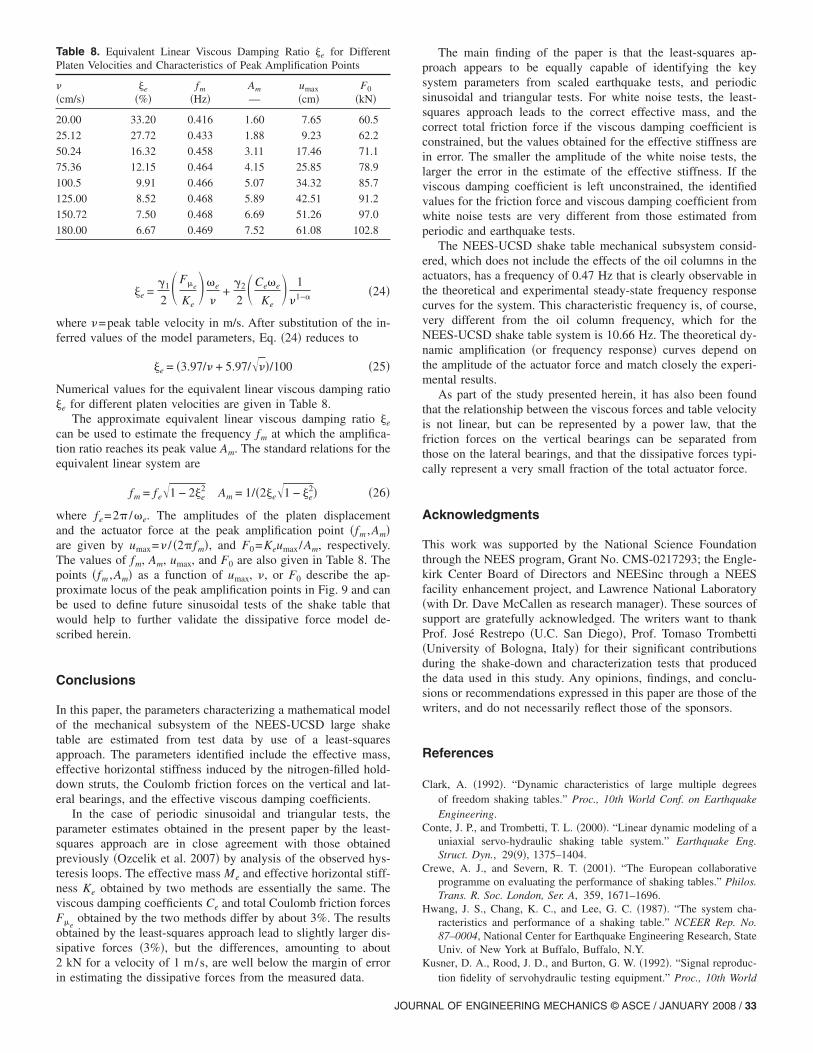
Numerical values for the equivalent linear viscous damping ratioe for different platen velocities are given in Table 8.

The approximate equivalent linear viscous damping ratio e

can be used to estimate the frequency fm at which the amplifica-tion ratio reaches its peak value Am. The standard relations for theequivalent linear system are

fm = fe�1 − 2e

2 Am = 1/�2e�1 − e

2� �26�

where fe=2� /�e. The amplitudes of the platen displacementand the actuator force at the peak amplification point �fm ,Am�are given by umax=� / �2�fm�, and F0=Keumax/Am, respectively.The values of fm, Am, umax, and F0 are also given in Table 8. Thepoints �fm ,Am� as a function of umax, �, or F0 describe the ap-proximate locus of the peak amplification points in Fig. 9 and canbe used to define future sinusoidal tests of the shake table thatwould help to further validate the dissipative force model de-scribed herein.

Conclusions

In this paper, the parameters characterizing a mathematical modelof the mechanical subsystem of the NEES-UCSD large shaketable are estimated from test data by use of a least-squaresapproach. The parameters identified include the effective mass,effective horizontal stiffness induced by the nitrogen-filled hold-down struts, the Coulomb friction forces on the vertical and lat-eral bearings, and the effective viscous damping coefficients.

In the case of periodic sinusoidal and triangular tests, theparameter estimates obtained in the present paper by the least-squares approach are in close agreement with those obtainedpreviously �Ozcelik et al. 2007� by analysis of the observed hys-teresis loops. The effective mass Me and effective horizontal stiff-ness Ke obtained by two methods are essentially the same. Theviscous damping coefficients Ce and total Coulomb friction forcesF�e

obtained by the two methods differ by about 3%. The resultsobtained by the least-squares approach lead to slightly larger dis-sipative forces �3%�, but the differences, amounting to about2 kN for a velocity of 1 m/s, are well below the margin of error

Table 8. Equivalent Linear Viscous Damping Ratio e for DifferentPlaten Velocities and Characteristics of Peak Amplification Points

��cm/s�

e

�%�fm

�Hz�Am

—umax

�cm�F0

�kN�

20.00 33.20 0.416 1.60 7.65 60.5

25.12 27.72 0.433 1.88 9.23 62.2

50.24 16.32 0.458 3.11 17.46 71.1

75.36 12.15 0.464 4.15 25.85 78.9

100.5 9.91 0.466 5.07 34.32 85.7

125.00 8.52 0.468 5.89 42.51 91.2

150.72 7.50 0.468 6.69 51.26 97.0

180.00 6.67 0.469 7.52 61.08 102.8

in estimating the dissipative forces from the measured data.

JOUR

The main finding of the paper is that the least-squares ap-proach appears to be equally capable of identifying the keysystem parameters from scaled earthquake tests, and periodicsinusoidal and triangular tests. For white noise tests, the least-squares approach leads to the correct effective mass, and thecorrect total friction force if the viscous damping coefficient isconstrained, but the values obtained for the effective stiffness arein error. The smaller the amplitude of the white noise tests, thelarger the error in the estimate of the effective stiffness. If theviscous damping coefficient is left unconstrained, the identifiedvalues for the friction force and viscous damping coefficient fromwhite noise tests are very different from those estimated fromperiodic and earthquake tests.

The NEES-UCSD shake table mechanical subsystem consid-ered, which does not include the effects of the oil columns in theactuators, has a frequency of 0.47 Hz that is clearly observable inthe theoretical and experimental steady-state frequency responsecurves for the system. This characteristic frequency is, of course,very different from the oil column frequency, which for theNEES-UCSD shake table system is 10.66 Hz. The theoretical dy-namic amplification �or frequency response� curves depend onthe amplitude of the actuator force and match closely the experi-mental results.

As part of the study presented herein, it has also been foundthat the relationship between the viscous forces and table velocityis not linear, but can be represented by a power law, that thefriction forces on the vertical bearings can be separated fromthose on the lateral bearings, and that the dissipative forces typi-cally represent a very small fraction of the total actuator force.

Acknowledgments

This work was supported by the National Science Foundationthrough the NEES program, Grant No. CMS-0217293; the Engle-kirk Center Board of Directors and NEESinc through a NEESfacility enhancement project, and Lawrence National Laboratory�with Dr. Dave McCallen as research manager�. These sources ofsupport are gratefully acknowledged. The writers want to thankProf. José Restrepo �U.C. San Diego�, Prof. Tomaso Trombetti�University of Bologna, Italy� for their significant contributionsduring the shake-down and characterization tests that producedthe data used in this study. Any opinions, findings, and conclu-sions or recommendations expressed in this paper are those of thewriters, and do not necessarily reflect those of the sponsors.

References

Clark, A. �1992�. “Dynamic characteristics of large multiple degreesof freedom shaking tables.” Proc., 10th World Conf. on EarthquakeEngineering.

Conte, J. P., and Trombetti, T. L. �2000�. “Linear dynamic modeling of auniaxial servo-hydraulic shaking table system.” Earthquake Eng.Struct. Dyn., 29�9�, 1375–1404.

Crewe, A. J., and Severn, R. T. �2001�. “The European collaborativeprogramme on evaluating the performance of shaking tables.” Philos.Trans. R. Soc. London, Ser. A, 359, 1671–1696.

Hwang, J. S., Chang, K. C., and Lee, G. C. �1987�. “The system cha-racteristics and performance of a shaking table.” NCEER Rep. No.87–0004, National Center for Earthquake Engineering Research, StateUniv. of New York at Buffalo, Buffalo, N.Y.

Kusner, D. A., Rood, J. D., and Burton, G. W. �1992�. “Signal reproduc-
tion fidelity of servohydraulic testing equipment.” Proc., 10th World

Conf. on Earthquake Engineering, Rotterdam, The Netherlands,2683–2688.

Ozcelik, O., Luco, E. J., Conte, J. P., Trombetti, T. L., and Restrepo, J. I.�2007�. “Experimental characterization, modeling and identification ofthe UCSD-NEES shake table mechanical system.” Earthquake Eng.Struct. Dyn., in press.

Rinawi, A. M., and Clough, R. W. �1991�. “Shaking table-structure inter-action.” EERC Rep. No. 91/13, Earthquake Engineering ResearchCenter, Univ. of California at Berkeley, Berkeley, Calif.

Shortreed, J. S., Seible, F., Filiatrault, A., and Benzoni, G. �2001�.“Characterization and testing of the Caltrans seismic response modi-fication device test system.” Philos. Trans. R. Soc. London, Ser. A,359, 1829–1850.

Thoen, B. K. �2004�. 469D seismic digital control software, MTSCorporation.

Thoen, B. K., and Laplace, P. N. �2004�. “Offline tuning of shaking


table.” Proc., 13th World Conf. on Earthquake Engineering, Vancou-ver, B. C., Canada, Aug. 1–6, Paper No. 960.

Trombetti, T. L., and Conte, J. P. �2002�. “Shaking table dynamics: Re-sults from a test analysis and comparison study.” J. Earthquake Eng.,6�4�, 513–551.

Twitchell, B. S., and Symans, M. D. �2003�. “Analytical modeling,system identification, and tracking performance of uniaxial seismicsimulators.” J. Eng. Mech., 129�12�, 1485–1488.

Van Den Einde, L., et al. �2004�. “Development of the George E. BrownJr. network for earthquake engineering simulation �NEES� large highperformance outdoor shake table at the Univ. of California, SanDiego.” Proc., 13th World Conf. on Earthquake Engineering, Vancou-ver, B.C., Canada, August 1–6, Paper No. 3,281.

Williams, D. M., Williams, M. S., and Blakeborough, A. �2001�. “Nu-merical modeling of a servohydraulic testing system for structures.”
J. Eng. Mech., 127�8�, 816–827.

Documents

Identification of the Mechanical Subsystem of the NEES-UCSD