Embed Size (px)
Citation preview

IDENTIFICATION OF SIMULTANEOUS EQUATIONS
MODEL ECONOMETRICS - II
COMPUTER PROJECT
19th April, 2013
Indira Gandhi Institute of Development Research
Shreya Bhattacharya
Sargam Jain
Saish Nevrekar
Deepak Kumar
OBJECTIVE
The objective of the project is to demonstrate the identification of simultaneous equations model for
sales and advertising relationships between filter and non-filter cigarette brands. The model tests for
the success of the participating tobacco companies in targeting the youth in the United States.
Motivation
Advertising is an important method of competition in industries that are highly concentrated, such as
the cigarette industry. Firms in industries of this type tend not to compete by price, but try to increase
sales with advertising and other marketing techniques. Since a number of prior studies have found little
relationship between advertising and tobacco consumption, it is important to examine this literature
before proceeding with a new empirical study. Economic theory provides some insights into how
econometric studies of tobacco advertising should be conducted. An important economic aspect of
advertising is diminishing marginal product. Diminishing marginal product suggests that, after some
point, additions to advertising will result in ever smaller additions to consumption. This concept is the
basis of the advertising response function. Advertising response functions have been used for some time
in brand level research to illustrate the effect of advertising at various levels on consumption.
Many of the recent advertising exposure and recall studies have controlled for other risk factors for
smoking initiation. This means that the alleged causal factor of advertising should be isolated from other
risk factors so that a genuine association can be determined. For instance, it might be true that 16-year-
olds who can remember tobacco advertisements are more likely to smoke as 20-year-olds than 16-year-
olds who do not remember tobacco advertisements, but it does not follow from this that this
association is due to the fact that they remembered tobacco advertisements. It might well be that those
16-year-olds might also have shared some other characteristic such as being more inclined to risk-
taking, or performing poorly at school, and it may be that these factors - which have been excluded from
most studies - rather than tobacco advertisements, are the cause(s) of subsequent smoking. The point is
that without controlling for these other factors one can never know.
Many of the recall studies are rendered problematic by the fact that they assume that the direction of
influence between advertising and smoking uptake and consumption is one-way. That is, they assume
that the reputedly causal direction is from exposure to advertising. Yet there is very little empirical
support offered for this. Indeed, important studies have contradicted it. Adolescents who are interested
in and receptive to smoking can be assumed to have a smoking preference that would lead to their
interest in and recall of tobacco advertising. Their preference for smoking could have been formed prior
to and independently of any tobacco advertisement. This would mean that discovering an association
between remembering tobacco advertisements and subsequently smoking does not constitute
compelling evidence that the former leads to the latter.
Moreover, tobacco advertising exposure and recall studies often rely on self-reported data, which poses
a significant problem in terms of validity. For instance, self-reported data may be inaccurate because of
certain situational factors associated with the social desirability of the behaviour, such as smoking, being
studied. The research literature notes that self-reports are often plagued by social desirability bias, that
is, subjects often report what they believe the interviewer wishes to hear or what is the socially
preferred option, rather than what is actually the case. Some studies have shown that the likelihood of
untruthful responses rises with the degree of threat posed by the question. But even setting aside the
question of conscious deception, there is the possibility of significant inaccuracy due to faulty recall.
Many tobacco advertising exposure and recall studies suffer from a variety of methodological issues
which undermine their internal validity. These include misspecified variances, omitted interactions and
paths, endogeneity, sample attrition and selection bias. As noted recently by Nelson, most longitudinal
studies of advertising exposure and recall fail to deal with these issues. (J. Nelson What is learned from
longitudinal studies of advertising and youth drinking and smoking? A critical assessment International
Journal of Environmental Research and Public Health20107:870-926.
Identification: A historical perspective
Intriligator (1978) defined identification as ‘the problem of relating the structural parameters of a
simultaneous equation model to the reduced-form parameters that "summarize all relevant information
available from the sample data"’. However, Bartel (1985) was the first to attempt a heuristic definition
of identification, where he claimed that identification was a problem that related directly to probabilistic
distributions. Identification has also been done in a Bayesian framework and for triangular simultaneous
equation systems for control variables (Imben and Newey, 2009). An interesting practical application of
the concept of identification has been in the case of standard auction models. Athey and Haile (2002)
present identification results for models of first-price, second-price, ascending and descending auctions.
Rigobon (2003) suggested an alternative method of identification by using the heteroscedasticity
present in the model. This method was used to measure the contemporaneous propagation between
the returns on several Latin American sovereign bonds. Berry formulated an alternative algorithm to
solve for identification, which is equivalent to the rank condition and simpler to evaluate.

Identification in simultaneous equations model:
A simultaneous equations system is defined as a system with two or more equations, where a variable
explained in one equation appears as an explanatory variable in another. Thus, the endogenous
variables in the system are simultaneously determined.
The Structural Form:
The structural form of the simultaneous equations system can be written as follows:
β’Yt+ Γ’ Xt=εt
Where:
β’- matrix of coefficients of endogenous variables of order (nxn)
Yt - vector of endogenous variables of order (nx1)
Γ’ - matrix of coefficients of exogenous variables of order (nxm)
Xt - vector of exogenous variables of order (mx1)
εt - vector of error terms of order (nx1)
The equations above are known as Structural or Behavioral Equations because they portray the
structure of an economy or the behavior of an economic agent. The β’ and Γ’ are known as structural
parameters or coefficients.
The Reduced Form:
The reduced form for simultaneous equations system can be obtained as follows:
We know,
β’ Yt+ Γ’ Xt=εt
This can be rewritten as:
β’ Yt= - Γ’ Xt+ εt
Since β’ is a non-singular matrix [i.e det (β’) is not equal to zero], it is invertible, thus:
Yt= - (β’)-1 Γ’Xt + (β’)-1εt
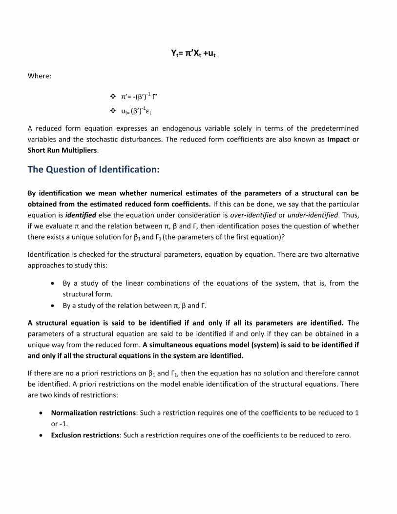
Yt= π’Xt +ut
Where:
π’= -(β’)-1 Γ’
ut= (β’)-1εt
A reduced form equation expresses an endogenous variable solely in terms of the predetermined
variables and the stochastic disturbances. The reduced form coefficients are also known as Impact or
Short Run Multipliers.
The Question of Identification:
By identification we mean whether numerical estimates of the parameters of a structural can be
obtained from the estimated reduced form coefficients. If this can be done, we say that the particular
equation is identified else the equation under consideration is over-identified or under-identified. Thus,
if we evaluate π and the relation between π, β and Γ, then identification poses the question of whether
there exists a unique solution for β1 and Γ1 (the parameters of the first equation)?
Identification is checked for the structural parameters, equation by equation. There are two alternative
approaches to study this:
By a study of the linear combinations of the equations of the system, that is, from the
structural form.
By a study of the relation between π, β and Γ.
A structural equation is said to be identified if and only if all its parameters are identified. The
parameters of a structural equation are said to be identified if and only if they can be obtained in a
unique way from the reduced form. A simultaneous equations model (system) is said to be identified if
and only if all the structural equations in the system are identified.
If there are no a priori restrictions on β1 and Γ1, then the equation has no solution and therefore cannot
be identified. A priori restrictions on the model enable identification of the structural equations. There
are two kinds of restrictions:
Normalization restrictions: Such a restriction requires one of the coefficients to be reduced to 1
or -1.
Exclusion restrictions: Such a restriction requires one of the coefficients to be reduced to zero.

Rank and Order Conditions for Identification:
Rank Condition:
To derive a unique solution for β* from the reduced form model:
r (πΔΔ*)=r[πΔΔ* πΔΔ1]=n*.
This condition is both a necessary as well as a sufficient condition.
Order Condition:
For the rank condition to hold the following order condition is a necessary condition:
mΔΔ≥n*
Where:
mΔΔ represents the number of excluded exogenous variables from the equation.
n* represents the number of included endogenous explanatory variables.
This implies that there should be sufficient enough exogenous variables to control for the
simultaneously changing endogenous variables. This implies that:
mΔΔ + mΔ ≥ n*+ mΔ => m ≥ n*+ mΔ
If mΔΔ< n* => Equation is not identified
If mΔΔ= n* => Equation is exactly identified (assuming that the rank condition is satisfied)
If mΔΔ>n* => Equation is overidentified (assuming that the rank condition is satisfied)
Reduced form Identification:
To determine the identification of the first equation in the simultaneous equation system:

Step1: Let Y1 be the explained variable in the first equation, normalize the coefficient attached to this
variable equal to -1.
Step 2: Let there be n* endogenous explanatory variables in the first equation (Y2, Y3, Y4 .......Yn*+1).
Partition Y= [Y1 Y* Y**]
Where:
Y1 is the (Tx1) matrix of the explained variable.
Y* is the (Txn*) matrix of endogenous explanatory variables that appear in the first equation.
Y** is the (Txn**) matrix of endogenous variables that do not appear in the first equation.
Total number of endogenous variables: n=1+n*+n**
Step3: Let there be mΔ exogenous explanatory variables in the first equation:
Partition X= [XΔ XΔΔ]
Where:
XΔ is the (TxmΔ) matrix of exogenous explanatory variables that appear in the first equation.
XΔΔ is the (TxmΔΔ) matrix of exogenous variables that do not appear in the first equation.
Total number of exogenous variables: m= mΔ + mΔΔ
Step 4: Now partition β1 and Γ1 accordingly:
β1= (
)
Γ1= ( )
Step 5: Now the first equation, Yβ1+XΓ1=ε1 can be written as:
(
) + ( ) = ε1
-Y1+Y*β*+XΔΓΔ= ε1
Step 6: Consider the reduced form: πβ= -Γ1
(
) = ( )
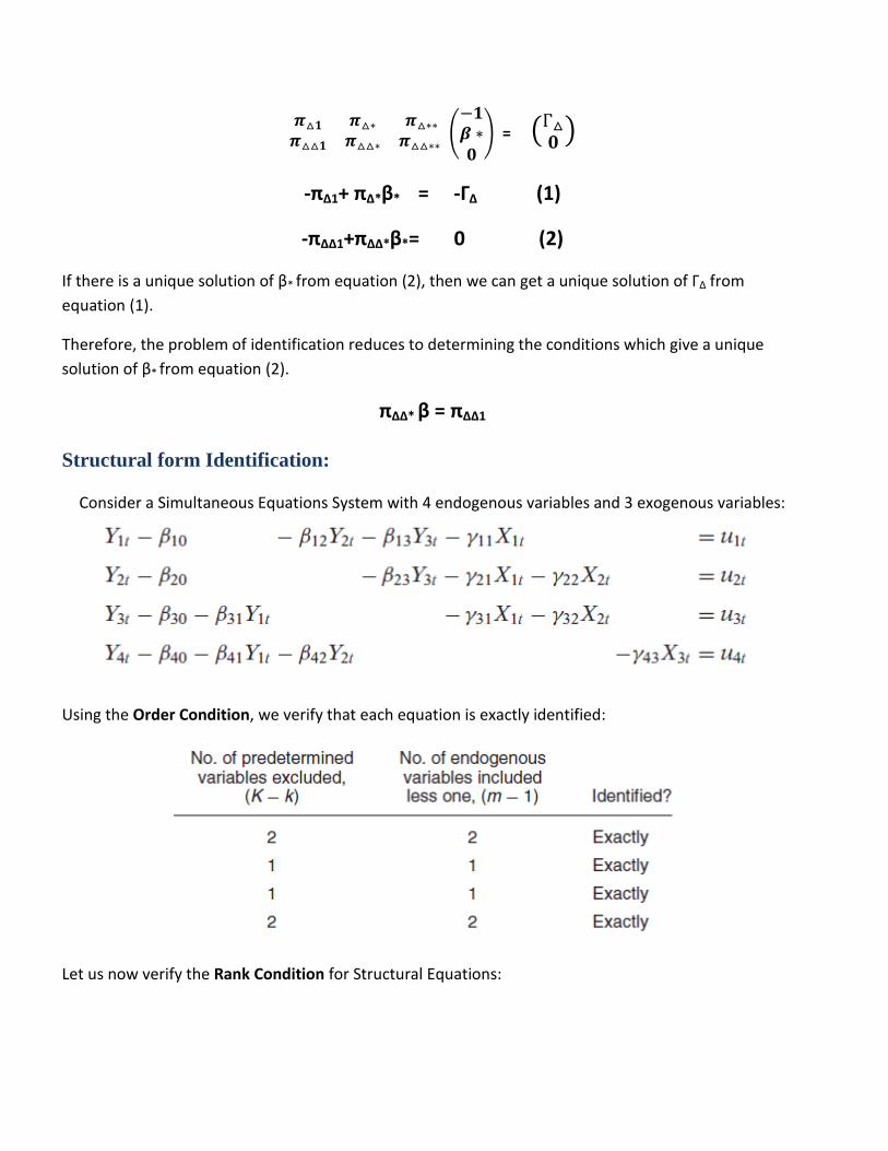
-πΔ1+ πΔ*β* = -ΓΔ (1)
-πΔΔ1+πΔΔ*β*= 0 (2)
If there is a unique solution of β* from equation (2), then we can get a unique solution of ΓΔ from
equation (1).
Therefore, the problem of identification reduces to determining the conditions which give a unique
solution of β* from equation (2).
πΔΔ* β = πΔΔ1
Structural form Identification:
Consider a Simultaneous Equations System with 4 endogenous variables and 3 exogenous variables:
Using the Order Condition, we verify that each equation is exactly identified:
Let us now verify the Rank Condition for Structural Equations:

“In a model containing M equations in M endogenous variables, an equation is identified if and only if
atleast one non zero determinant of order (M-1)x(M-1) can be constructed from the coefficients of the
variables (both endogenous and predetermined) excluded from that particular equation but included in
the other equations of the model.”
Consider the first equation which excludes the variables Y4, X2, X3. For this equation to be identified we
must obtain at least one non-zero determinant of order 3x3 from the coefficients of the variables
excluded from this equation but included in other equations. The rank condition of the other equations
will also follow in the same manner. In case, such a matrix is not found or the determinant of the matrix
is equal to zero, the particular equation is unidentified. Consequently, the system of equations will also
be unidentified.
The Model:
The model studies the expenditure on cigarette advertisements in national newspapers, magazines and
promotional billboards in USA over a period of 1952- 1965. The model focuses on those modes of
advertisement which are closely targeted by the population above the age of 20 years.
The model consists of two demand equations for two competing groups of cigarette brands and two
equations that describe the advertising relations of these groups of brands. The sales of the major filter
cigarette brands have been aggregated to give one demand equation for this group. Similarly, there is
one demand equation for the major non-filter brands.
Since the prices of filter brands are identical as are the prices of non-filter brands, the aggregation of
brand sales in each class is justified theoretically. The Leontieff-Hick’s Theorem establishes that if the
prices of a group of goods change in equal proportion, that group can then be treated as a single
commodity. Since, this theorem justifies aggregation in this study; the concepts of complementarity,

substitutability, price elasticity, income elasticity apply to the grouped commodities just as the
corresponding concepts and measures apply to single goods.
Variables used in the model:
Log (Salesft): Logarithm of sales for filter cigarettes divided by population over age 20.
Log (Adft): Logarithm of advertising dollar sales for filter cigarettes divided by population over age
20.
Log (Adnft): Logarithm of advertising dollar sales for non-filter cigarettes divided by population
over age 20.
Log (PDIt): Logarithm of disposable personal income divided by population over age 20 divided by
consumer price index.
Log (Pricet): Logarithm of price per package of non-filter divided by consumer price
index.
Log (Salesnft): Logarithm of sales for non-filter cigarettes divided by population over age 20.
Demand for Major Brands of Filter and Non-Filter Cigarettes:
Demand Equation for Filter Brands:
For every year t, demand for filter brands is considered in isolation from the rest of the system,
Log(Salesft)= Log(Adft)+ Log(Adnft)+ Log(PDIt)+ Log(Pricet)+ εt
We therefore postulate that the per capita sales of filter cigarettes is a non-linear function function of
the ratio of per capita advertising for the two competitive types of cigarettes and the two exogenous
variables. Although it might have been desirable to include prices of the filter and non-filter cigarettes as
variables, the non-filter price is available as a component of CPI but the filter price is not.
Demand Equation for Non-Filter Brands:
For every year t, demand for Non-filter brands is considered in isolation from the rest of the system,
Log(Salesnft)= Log(Adft)+ Log(Adnft)+ Log(PDIt)+ Log(Pricet)+ ε2t
Advertising Relationships for Major Brands of Filter and Non-Filter Cigarettes:
Equation describing Advertising Behaviour of Filter Brands:

Log (Salesft) = Log(Salesnft)+ Log(Adft)+ ε3t
Equation describing Advertising Behaviour of Non-Filter Brands:
Log (Salesnft)= Log(Salesft)+ Log(Adnft)+ ε4t
Model of Sales and Advertising of Filter and Non-Filter Cigarettes:
The model’s parts produce the system of structural equations that describe the sales and
advertising of the two competing products:
-Log(Salesft)+0.Log (Salesnft)+ Log(Adft)+ Log(Adnft)+ Log(PDIt)+ Log(Pricet)+ ε1t =0
0.Log (Salesft)-Log(Salesnft)+ Log(Adft)+ Log(Adnft)+ Log(PDIt)+ Log(Pricet)+ ε2t =0
-Log (Salesft) + Log (Salesnft) + Log(Adft)+0.Log (Adnft)+ 0. Log (PDIt) + 0. Log (Pricet)+ε3t =0
Log (Salesft) – Log (Salesnft) + 0.Log (Adft) + Log (Adnft) + 0. Log (PDIt) + 0. Log (Pricet)+ε4t
=0
The reduced form equations for this system are:
Log (Salesft)= Log(PDIt)+ Log(Pricet)+ ε1t
Log (Salesnft)= Log(PDIt)+ Log(Pricet)+ ε2t
Log (Adft)= Log (PDIt)+ Log(Pricet)+ε3t
Log (Adnft)= Log (PDIt)+ Log(Pricet)+ε4t
Under certain circumstances the structural parameters may be estimated without testing the model;
However if the structural equations are unidentified or over-identified, estimation procedures are
debatable.
IDENTIFICATION OF THE MODEL USING SAS:
Commands used in SAS:
proc syslin data= sasuser.data1 3sls;
endogenous salesf salesnf adf adnf;
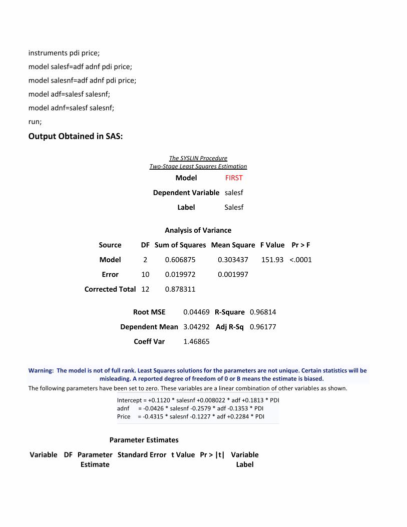
instruments pdi price;
model salesf=adf adnf pdi price;
model salesnf=adf adnf pdi price;
model adf=salesf salesnf;
model adnf=salesf salesnf;
run;
Output Obtained in SAS:
The SYSLIN Procedure Two-Stage Least Squares Estimation
Model FIRST
Dependent Variable salesf
Label Salesf
Analysis of Variance
Source DF Sum of Squares Mean Square F Value Pr > F
Model 2 0.606875 0.303437 151.93 <.0001
Error 10 0.019972 0.001997
Corrected Total 12 0.878311
Root MSE 0.04469 R-Square 0.96814
Dependent Mean 3.04292 Adj R-Sq 0.96177
Coeff Var 1.46865
Warning: The model is not of full rank. Least Squares solutions for the parameters are not unique. Certain statistics will be misleading. A reported degree of freedom of 0 or B means the estimate is biased.
The following parameters have been set to zero. These variables are a linear combination of other variables as shown.
Intercept = +0.1120 * salesnf +0.008022 * adf +0.1813 * PDI adnf = -0.0426 * salesnf -0.2579 * adf -0.1353 * PDI Price = -0.4315 * salesnf -0.1227 * adf +0.2284 * PDI
Parameter Estimates
Variable DF Parameter Estimate
Standard Error t Value Pr > |t| Variable Label
Parameter Estimates
Variable DF Parameter Estimate
Standard Error t Value Pr > |t| Variable Label
Intercept 0 0 . . . Intercept
salesnf 0 -0.20442 0.440859 -0.46 0.6528 salesnf
Adf 0 0.702683 0.245282 2.86 0.0168 Adf
Adnf 0 0 . . . Adnf
PDI 0 1.164988 0.389058 2.99 0.0135 PDI
Price 0 0 . . . Price
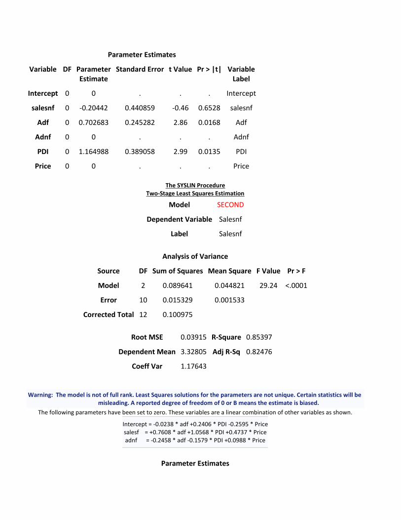
The SYSLIN Procedure
Two-Stage Least Squares Estimation
Model SECOND
Dependent Variable Salesnf
Label Salesnf
Analysis of Variance
Source DF Sum of Squares Mean Square F Value Pr > F
Model 2 0.089641 0.044821 29.24 <.0001
Error 10 0.015329 0.001533
Corrected Total 12 0.100975
Root MSE 0.03915 R-Square 0.85397
Dependent Mean 3.32805 Adj R-Sq 0.82476
Coeff Var 1.17643
Warning: The model is not of full rank. Least Squares solutions for the parameters are not unique. Certain statistics will be misleading. A reported degree of freedom of 0 or B means the estimate is biased.
The following parameters have been set to zero. These variables are a linear combination of other variables as shown.
Intercept = -0.0238 * adf +0.2406 * PDI -0.2595 * Price salesf = +0.7608 * adf +1.0568 * PDI +0.4737 * Price adnf = -0.2458 * adf -0.1579 * PDI +0.0988 * Price
Parameter Estimates
Variable DF Parameter Estimate
Standard Error t Value Pr > |t| Variable Label
Intercept 0 0 . . . Intercept
salesf 0 0 . . . salesf
Adf 0 -0.28426 0.110870 -2.56 0.0282 adf
adnf 0 0 . . . adnf
PDI 0 0.529357 0.136513 3.88 0.0031 PDI
Price 0 -2.31738 0.895048 -2.59 0.0270 Price
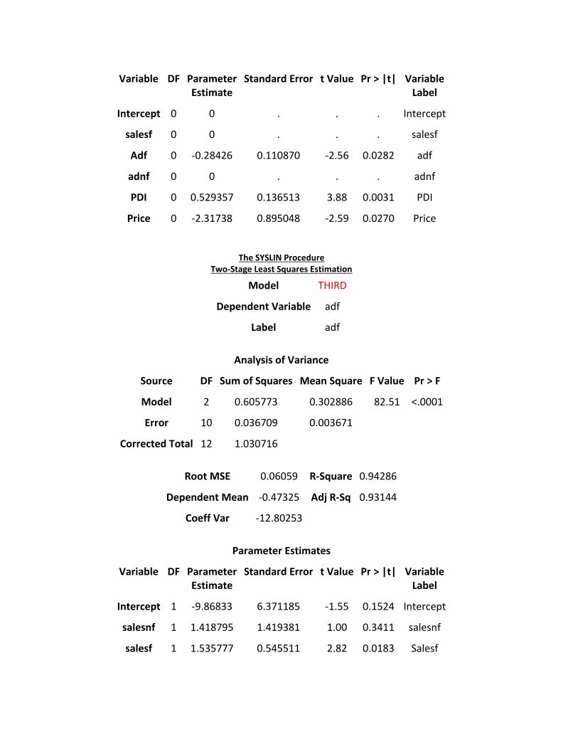
The SYSLIN Procedure Two-Stage Least Squares Estimation
Model THIRD
Dependent Variable adf
Label adf
Analysis of Variance
Source DF Sum of Squares Mean Square F Value Pr > F
Model 2 0.605773 0.302886 82.51 <.0001
Error 10 0.036709 0.003671
Corrected Total 12 1.030716
Root MSE 0.06059 R-Square 0.94286
Dependent Mean -0.47325 Adj R-Sq 0.93144
Coeff Var -12.80253
Parameter Estimates
Variable DF Parameter Estimate
Standard Error t Value Pr > |t| Variable Label
Intercept 1 -9.86833 6.371185 -1.55 0.1524 Intercept
salesnf 1 1.418795 1.419381 1.00 0.3411 salesnf
salesf 1 1.535777 0.545511 2.82 0.0183 Salesf

The SYSLIN Procedure Two-Stage Least Squares Estimation
Model FOURTH
Dependent Variable Adnf
Label Adnf
Analysis of Variance
Source DF Sum of Squares Mean Square F Value Pr > F
Model 2 0.043281 0.021641 37.60 <.0001
Error 10 0.005755 0.000576
Corrected Total 12 0.086330
Root MSE 0.02399 R-Square 0.88264
Dependent Mean -0.49102 Adj R-Sq 0.85916
Coeff Var -4.88565
Parameter Estimates
Variable DF Parameter Estimate
Standard Error t Value Pr > |t| Variable Label
Intercept 1 1.739523 2.522642 0.69 0.5062 Intercept
salesnf 1 -0.31649 0.561998 -0.56 0.5857 salesnf
IDENTIFICATION OF THE MODEL USING STATA:
The conventional order condition (necessary but not sufficient) pertaining to single-equation estimation
with instrumental variables is satisfied by counting included endogenous and excluded exogenous
variables in the equation. The sufficient rank condition pertains to the rank of the matrix of instruments.
At present, Stata's reg3 command does not check to see that the conditions for identification of a
structural system are satisfied, and produces estimation results. The checkreg3 command allows you
to verify that these results are meaningful by checking to see that the rank condition is satisfied for each
of the N equations in the system. Unless the rank condition is satisfied for each equation in the system,

Rank deficiency: System is not identified Eq 4 fails rank condition for identificationEq 3 fails rank condition for identificationEq 2 fails rank condition for identificationEq 1 fails rank condition for identification logadnf 0 0 logadf 0 0logsalesnf .5 .5 logsalesf .5 .5 logpdi logprice
Exogenous coefficients matrix
logadnf .5 .5 0 -1 logadf .5 .5 -1logsalesnf 0 -1 logsalesf -1 logsalesf logsalesnf logadf logadnf
Endogenous coefficients matrix
> alesnf)> gadnf logpdi logprice) ( logadf logsalesf logsalesnf) ( logadnf logsalesf logs. checkreg3 ( logsalesf logadf logadnf logpdi logprice) ( logsalesnf logadf lo
the system is unidentified. Although unusual for a system to satisfy the order condition without
satisfying the rank condition, it can occur.
Regression Results with CheckReg3:
SUMMARY AND CONCLUSION:
From the above studied model on sales and advertising expenditure of cigarettes, it can be seen that
each of the equations violate the Rank Condition necessary for identification as some of the parameters
in each of the structural equations do not have unique solutions. In the simultaneous model specified
above the following structural parameters remain unidentified:
Since, the model is not of full rank, the Least Squares solutions for the parameters are not unique. The
estimates obtained will be misleading. There is possible biasedness of estimates.
Despite its limitations, the simultaneous equation regression model can be successfully applied to advertising
problems and may aid in shaping managerial decisions. Estimates of the unidentified structural parameters have
been developed by two stage least squares regression, but the significance of this estimation has not been
determined.

Bibliography
Gujarati D. Basic Econometrics (4ed., MGH, 2004);
Wooldridge J.M. Introductory econometrics (South-Western College Pub., 2003);
Lecture Notes- Subrata Sarkar, IGIDR, Mumbai;
Advertising Publications, Inc., "Costs of Cigarette Advertising: 1952-1959," Advertising Age, 31
(September 19, 1960), 126-127;
"Costs of Cigarette Advertising: 1957-1965," Advertising Age, 37 (July 25, 1966), 56-58;
U.S. Census Bureau, Statistical Abstract of United States, Washington, D.C.: Government Printing Office,
1965, 327; 360-1;
http://data.worldbank.org/

Appendix
Commands Used:
SAS:
proc syslin data= sasuser.data1 3sls;
endogenous salesf salesnf adf adnf;
instruments pdi price;
model salesf=adf adnf pdi price;
model salesnf=adf adnf pdi price;
model adf=salesf salesnf;
model adnf=salesf salesnf;
run;
STATA:
Checkreg3 (LogSalesf LogAdf LogAdnf LogPDI LogPrice) (LogSalesnf LogAdf LogAdnf LogPDI LogPrice) (LogAdf
LogSalesf LogSalesnf) (LogAdnf LogSalesf LogSalesnf)
Data Sources:
The data used in the study was available from the year 1953 to 1965.
YEAR LOG(SALESF) LOG(SALESNF) LOG(ADF) LOG(ADNF) LOG(PDI) LOG(PRICE)
1953 2.39851 3.50465 -1.26117 -0.28369 3.41653 -0.60906
1954 2.6006 3.45582 -0.90035 -0.37119 3.41876 -0.60906
1955 2.8389 3.42632 -0.62703 -0.43061 3.44491 -0.60206
1956 2.97883 3.38979 -0.43572 -0.44389 3.46147 -0.60033
1957 3.09065 3.3381 -0.34364 -0.55378 3.46451 -0.59176
1958 3.15067 3.30278 -0.34605 -0.53839 3.46304 -0.5986
1959 3.18361 3.30251 -0.3051 -0.54141 3.47986 -0.57349
1960 3.19626 3.2992 -0.33548 -0.53467 3.48502 -0.57675
1961 3.20779 3.29484 -0.34157 -0.54432 3.49358 -0.57675

1962 3.21945 3.27891 -0.36206 -0.54872 3.50804 -0.5784
1963 3.23843 3.2572 -0.28542 -0.5458 3.51834 -0.56543
1964 3.22329 3.20154 -0.29571 -0.54809 3.54063 -0.55596
1965 3.23099 3.21304 -0.31297 -0.49872 3.56335 -0.5391
The data obtained on the sales of filter cigarettes was an aggregation over the following brands: WINSTON, KENT,
MARLBORO, HERBERT TAREYTON, VICEROY, L&M and Parliament. The data on sales of non-filter cigarettes
include the following brands: Pall Mall, Camel, Lucky Strike, Chester Field, Old Gold and Philip Moris.