Identification of Robust Biomarkers using the Biomarker Meta-

Analysis Module

By: Jasmine Chong, Jeff Xia

Date: 14/02/2018

The aim of this tutorial is to demonstrate how the Biomarker Meta-Analysis module of

MetaboAnalyst can be used to identify robust and novel biomarkers of disease/other conditions

through the integration of individual metabolomics studies. The example data used in this tutorial

comes from a subset of GCTOFMS data deposited in the Metabolomics Workbench from Fiehn et al.

2016 (doi: 10.21228/M85P57) which has been slightly modified to demonstrate the full capabilities

of this module. The primary objective of their study is to identify biomarkers of adenocarcinoma

(lung cancer) in blood.

Introduction to Biomarker Meta-Analysis

Biomarker identification is an important area of research in metabolomics, and their validation is

challenging due to inconsistencies in identified biomarkers amongst similar experiments. With the

wide application of metabolomics and the establishment of several metabolomics data repositories,

there is an ever-increasing interest to perform secondary analysis of published metabolomics datasets

collected under similar study conditions in similar populations, a practice often referred to as “meta-

analysis”. When executed properly, meta-analysis can leverage the collective power of multiple

studies to overcome study biases and small effect sizes to improve the precision in identifying true

patterns and robust biomarkers within data. The primary goal of the Biomarker Meta-Analysis

module is to provide a user-friendly tool for the integration of individual metabolomics studies to

identify robust biomarkers. The main steps for Biomarker Meta-Analysis are as following and will be

described in further detail:

i. Upload individual datasets. Prior to uploading the data, clean the datasets to ensure

consistency amongst feature names (compound IDs, spectral bins, or peaks) as well as

consistency in the class labels across all included studies.

ii. The module will perform differential enrichment analysis for each individual study to

compute summary level-statistics for each metabolite feature (e.g. p-value).

iii. The summary level-statistical results from all studies are combined, and meta-analysis is

performed using one of several statistical options: combining of p-values, vote counting, or

direct merging for very similar datasets.

iv. The results can be visualized as a Venn diagram to view all possible combinations of shared

features between the datasets.

Data Upload Preparation

Before uploading your data to the module, please make sure that the names of your features

(compound names, spectral bins, peaks) are consistent between the individual studies. At least 25%

of the features must match between the studies. Also make sure that the group labels are also

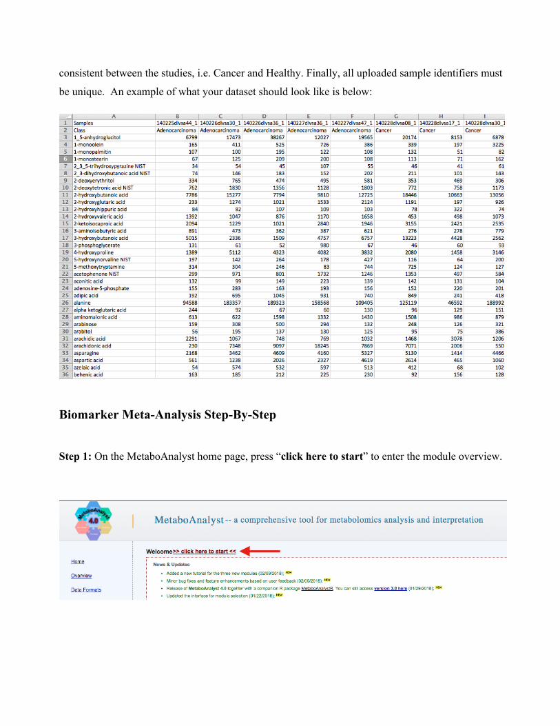
consistent between the studies, i.e. Cancer and Healthy. Finally, all uploaded sample identifiers must

be unique. An example of what your dataset should look like is below:

Biomarker Meta-Analysis Step-By-Step

Step 1: On the MetaboAnalyst home page, press “click here to start” to enter the module overview.

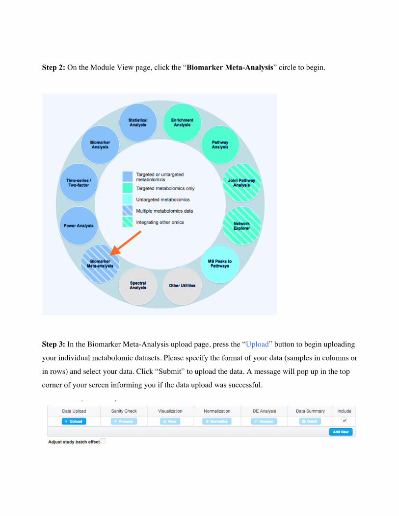
Step 2: On the Module View page, click the “Biomarker Meta-Analysis” circle to begin.

Step 3: In the Biomarker Meta-Analysis upload page, press the “Upload” button to begin uploading

your individual metabolomic datasets. Please specify the format of your data (samples in columns or

in rows) and select your data. Click “Submit” to upload the data. A message will pop up in the top

corner of your screen informing you if the data upload was successful.

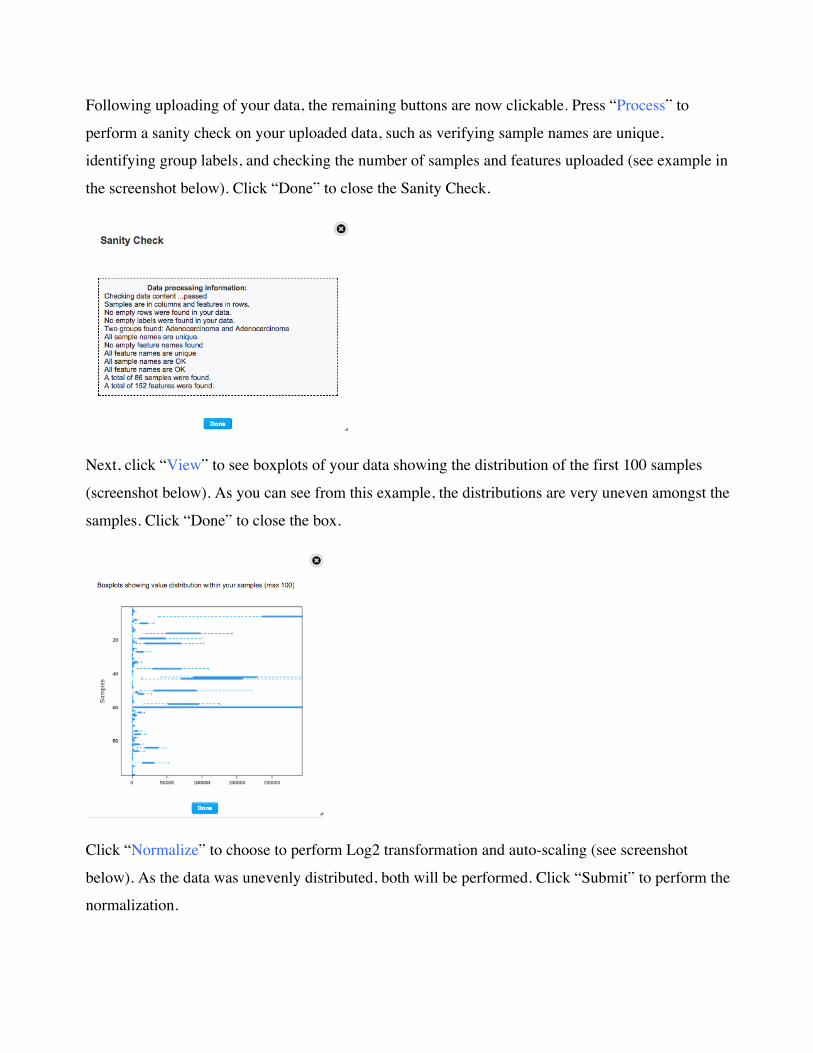
Following uploading of your data, the remaining buttons are now clickable. Press “Process” to

perform a sanity check on your uploaded data, such as verifying sample names are unique,

identifying group labels, and checking the number of samples and features uploaded (see example in

the screenshot below). Click “Done” to close the Sanity Check.

Next, click “View” to see boxplots of your data showing the distribution of the first 100 samples

(screenshot below). As you can see from this example, the distributions are very uneven amongst the

samples. Click “Done” to close the box.

Click “Normalize” to choose to perform Log2 transformation and auto-scaling (see screenshot

below). As the data was unevenly distributed, both will be performed. Click “Submit” to perform the

normalization.

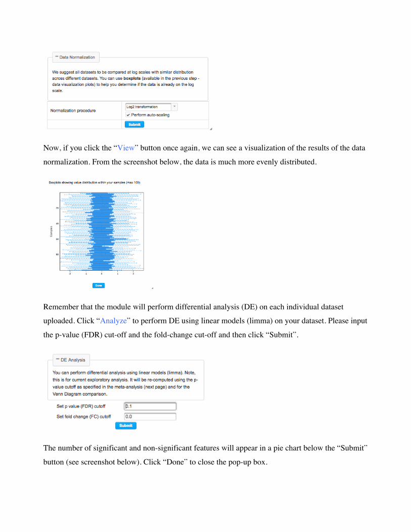
Now, if you click the “View” button once again, we can see a visualization of the results of the data

normalization. From the screenshot below, the data is much more evenly distributed.

Remember that the module will perform differential analysis (DE) on each individual dataset

uploaded. Click “Analyze” to perform DE using linear models (limma) on your dataset. Please input

the p-value (FDR) cut-off and the fold-change cut-off and then click “Submit”.

The number of significant and non-significant features will appear in a pie chart below the “Submit”

button (see screenshot below). Click “Done” to close the pop-up box.

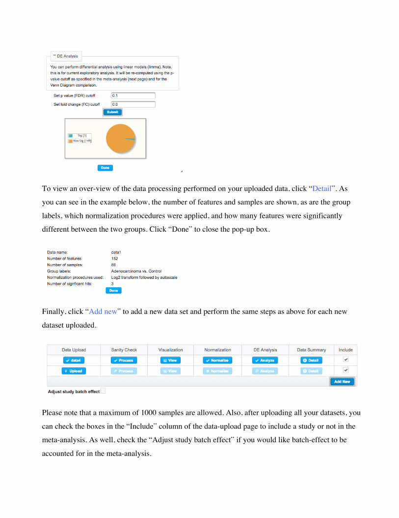
To view an over-view of the data processing performed on your uploaded data, click “Detail”. As

you can see in the example below, the number of features and samples are shown, as are the group

labels, which normalization procedures were applied, and how many features were significantly

different between the two groups. Click “Done” to close the pop-up box.

Finally, click “Add new” to add a new data set and perform the same steps as above for each new

dataset uploaded.

Please note that a maximum of 1000 samples are allowed. Also, after uploading all your datasets, you

can check the boxes in the “Include” column of the data-upload page to include a study or not in the

meta-analysis. As well, check the “Adjust study batch effect” if you would like batch-effect to be

accounted for in the meta-analysis.

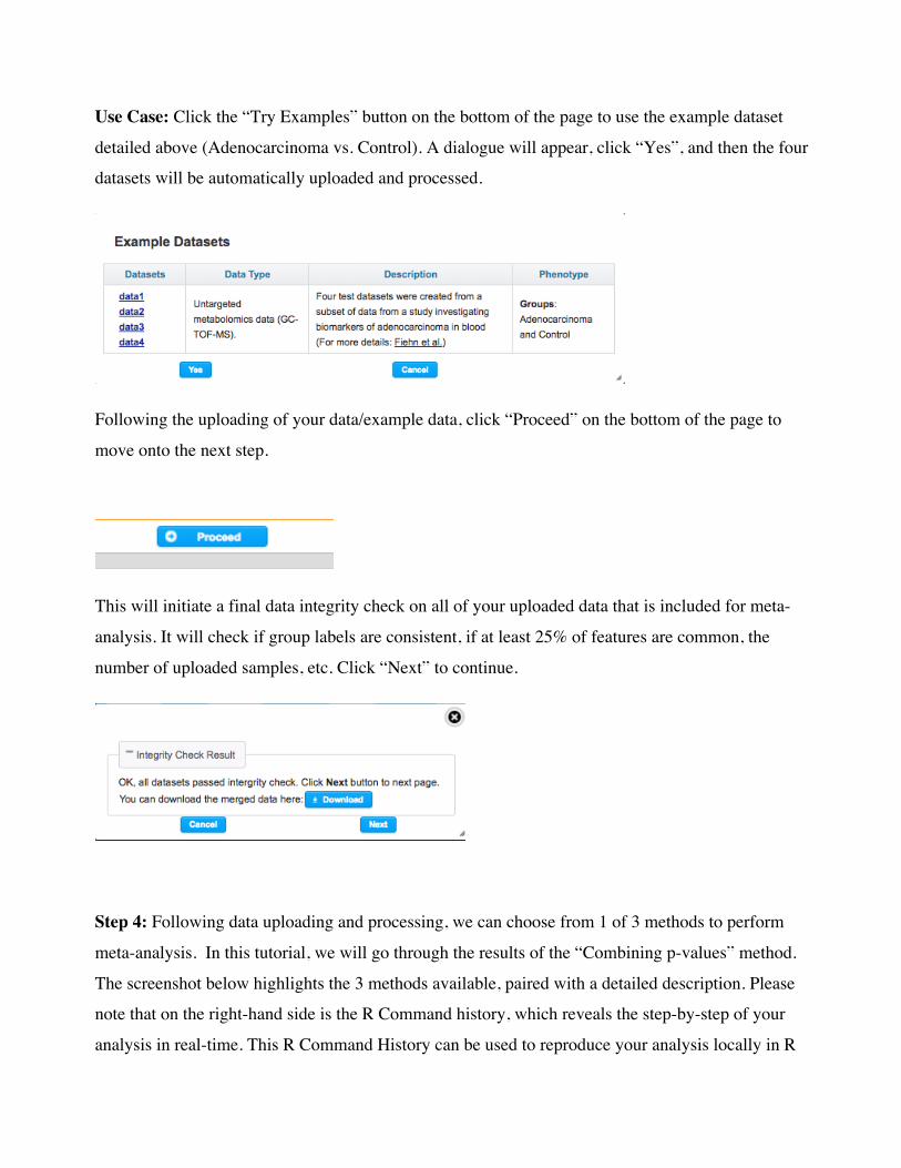
Use Case: Click the “Try Examples” button on the bottom of the page to use the example dataset

detailed above (Adenocarcinoma vs. Control). A dialogue will appear, click “Yes”, and then the four

datasets will be automatically uploaded and processed.

Following the uploading of your data/example data, click “Proceed” on the bottom of the page to

move onto the next step.

This will initiate a final data integrity check on all of your uploaded data that is included for meta-

analysis. It will check if group labels are consistent, if at least 25% of features are common, the

number of uploaded samples, etc. Click “Next” to continue.

Step 4: Following data uploading and processing, we can choose from 1 of 3 methods to perform

meta-analysis. In this tutorial, we will go through the results of the “Combining p-values” method.

The screenshot below highlights the 3 methods available, paired with a detailed description. Please

note that on the right-hand side is the R Command history, which reveals the step-by-step of your

analysis in real-time. This R Command History can be used to reproduce your analysis locally in R

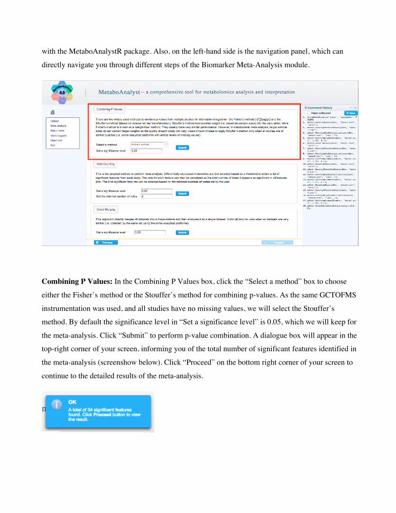
with the MetaboAnalystR package. Also, on the left-hand side is the navigation panel, which can

directly navigate you through different steps of the Biomarker Meta-Analysis module.

Combining P Values: In the Combining P Values box, click the “Select a method” box to choose

either the Fisher’s method or the Stouffer’s method for combining p-values. As the same GCTOFMS

instrumentation was used, and all studies have no missing values, we will select the Stouffer’s

method. By default the significance level in “Set a significance level” is 0.05, which we will keep for

the meta-analysis. Click “Submit” to perform p-value combination. A dialogue box will appear in the

top-right corner of your screen, informing you of the total number of significant features identified in

the meta-analysis (screenshow below). Click “Proceed” on the bottom right corner of your screen to

continue to the detailed results of the meta-analysis.

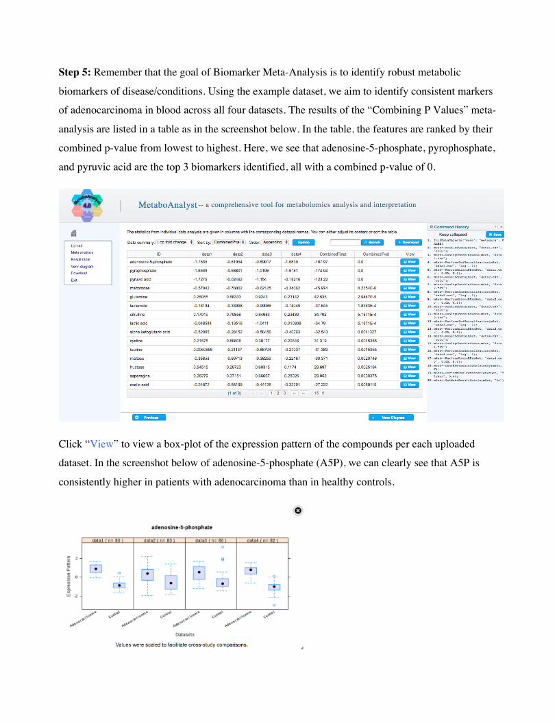
Step 5: Remember that the goal of Biomarker Meta-Analysis is to identify robust metabolic

biomarkers of disease/conditions. Using the example dataset, we aim to identify consistent markers

of adenocarcinoma in blood across all four datasets. The results of the “Combining P Values” meta-

analysis are listed in a table as in the screenshot below. In the table, the features are ranked by their

combined p-value from lowest to highest. Here, we see that adenosine-5-phosphate, pyrophosphate,

and pyruvic acid are the top 3 biomarkers identified, all with a combined p-value of 0.

Click “View” to view a box-plot of the expression pattern of the compounds per each uploaded

dataset. In the screenshot below of adenosine-5-phosphate (A5P), we can clearly see that A5P is

consistently higher in patients with adenocarcinoma than in healthy controls.

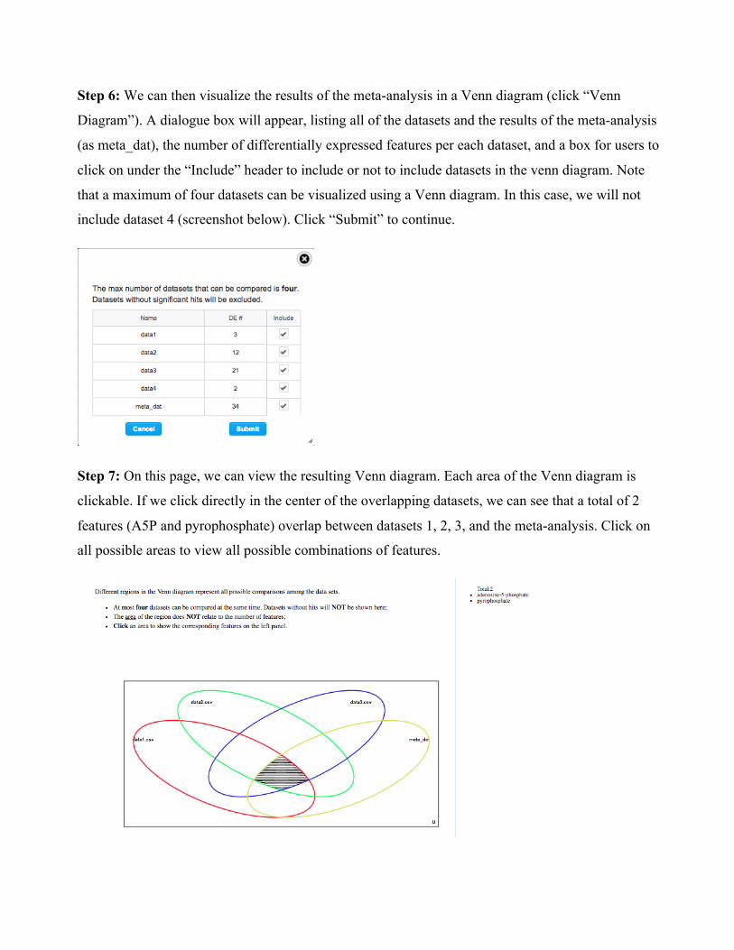
Step 6: We can then visualize the results of the meta-analysis in a Venn diagram (click “Venn

Diagram”). A dialogue box will appear, listing all of the datasets and the results of the meta-analysis

(as meta_dat), the number of differentially expressed features per each dataset, and a box for users to

click on under the “Include” header to include or not to include datasets in the venn diagram. Note

that a maximum of four datasets can be visualized using a Venn diagram. In this case, we will not

include dataset 4 (screenshot below). Click “Submit” to continue.

Step 7: On this page, we can view the resulting Venn diagram. Each area of the Venn diagram is

clickable. If we click directly in the center of the overlapping datasets, we can see that a total of 2

features (A5P and pyrophosphate) overlap between datasets 1, 2, 3, and the meta-analysis. Click on

all possible areas to view all possible combinations of features.

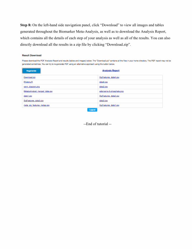
Step 8: On the left-hand side navigation panel, click “Download” to view all images and tables

generated throughout the Biomarker Meta-Analysis, as well as to download the Analysis Report,

which contains all the details of each step of your analysis as well as all of the results. You can also

directly download all the results in a zip file by clicking “Download.zip”.

--End of tutorial --