Identification of regions of fastest mixing in a system of point vortices

INTERNATIONAL JOURNAL FOR NUMERICAL METHODS IN FLUIDSInt. J. Numer. Meth. Fluids 2002; 38:447–469 (DOI: 10.1002/�d.130)

Identi&cation of regions of fastest mixing in a systemof point vortices

Prabhu Ramachandran and S. C. Rajan∗;†

Department of Aerospace Engineering; Indian Institute of Technology Madras; Chennai; India

SUMMARY

This paper describes a numerical method for e:ciently identifying the regions of fastest mixing ofa passive dye in a �ow due to a system of point vortices. Results obtained from computations arepresented for systems of three and four point vortices, both in the unbounded domain and inside acircular cylinder. The �ow is two-dimensional and the �uid is incompressible. The regions where mixingis possible are found by studying the largest Lagrangian Lyapunov exponent distribution with respectto various initial positions of tracer particles. The regions of fastest mixing are then identi&ed from theLyapunov exponent distribution at small times. The results of the method are veri&ed by quantifyingthe mixing by using a traditional box counting technique. The technique is then applied to severaldi?erent initial con&gurations of vortices and some interesting results are obtained. Some numerical&ndings about the nature of the exponents computed are also discussed. Copyright ? 2002 John Wiley& Sons, Ltd.

KEY WORDS: chaos; Lyapunov exponent; mixing; point vortices

1. INTRODUCTION

Understanding the phenomenon of mixing and the quantitative prediction of the rate of mixingis important and has a wide variety of applications in aerospace and chemical engineering.It is a well-known fact that e:cient mixing of �uids is intimately connected with chaos [1].Novikov [2] considered a system of three vortices as a model of two-dimensional turbulenceand obtained an exact solution to the problem of interaction of three identical vortices. Aref [3]presented an innovative qualitative analysis for the motion of three vortices having arbitrarystrengths. Aref and Pomphrey [4; 5] presented numerical evidence of chaos in four point vortexsystems and also showed formally that the three-vortex problem was integrable and that thefour-vortex problem is not. The recent work of Babiano et al. [6] is also concerned with chaosin point vortex systems. Their &nding is that irrespective of the fact that the velocity &elddisplays Eulerian chaos (it is to be noted here that such a velocity &eld implies that the vortexmotion is chaotic) or not, near the eye of the vortices there is regular Lagrangian motion,

∗Correspondence to: S. C. Rajan, Department of Aerospace Engineering, Indian Institute of Technology Madras,Chennai 600 036, India.

†E-mail: [email protected]

Received July 1999Copyright ? 2002 John Wiley & Sons, Ltd. Revised May 2000

448 R. PRABHU AND S. C. RAJAN

characterized by a null Lagrangian Lyapunov exponent. However, the issues of mixing arenot addressed in these articles. The mixing induced by a pair of &xed blinking vortices wasstudied by Aref [7]. The blinking vortices are point vortices that are alternately turned onand o?. This is similar to having two &xed rotating cylindrical stirrers that abruptly switchon and o?. Aref identi&ed di?erent conditions for e:cient mixing by placing blobs of tracerparticles and studying their advection. However, questions regarding the regions of high andlow mixing were not addressed. Franjione and Ottino [8] discuss the computational di:cultiesinvolved in numerically tracking the evolution of material lines in order to study mixing. Aref[9] provides an excellent review of the topic of vortex motion in two-dimensional �ows. Thequestion of e:cient identi&cation of regions of mixing is not addressed in these works.This paper is concerned with mixing in point vortex systems. A simple technique is pre-

sented to identify the regions of fastest mixing in such systems. Regions of mixing areidenti&ed by numerically calculating the distribution of the largest Lagrangian Lyapunov ex-ponent of the �ow with respect to the initial position of tracer particles for a given initialcon&guration of the point vortices. Subsequently, the regions of fastest mixing are identi&edby studying the exponent distribution at small times. Such a scheme is both easy to imple-ment and more e:cient than the traditional box counting schemes and a comparison betweenthe two is also presented in this work. It is to be noted that it would be extremely hard tocarry out an analytical study as performed by Aref for the motion of three vortices. A linearstability analysis is not of much use for such systems as one cannot &nd &xed points in the�ow for all times. Studying this system numerically, in which the particle paths are governedby ordinary di?erential equations (ODEs), is much easier. The method employed to identifythe regions of most e:cient mixing in the �ow is &rst described in detail with the help ofa three vortex problem, having a speci&c initial con&guration of the vortices. The methodis then applied to a few di?erent initial con&gurations of three and four vortices and someinteresting results are obtained. Henceforth the term ‘Lyapunov exponent’ will refer to thelargest Lagrangian Lyapunov exponent unless otherwise mentioned. From the computations itis found that when the vortices are constrained to move in a circular orbit, there are no regionsin the �ow where mixing is possible, and the Lyapunov exponents are all zero. When thisvortex con&guration is perturbed, regions of chaotic tracer motion gradually appear, having apositive Lyapunov exponent. These regions are interspersed with regular regions having a nullLyapunov exponent. As earlier reported by Babiano et al. [6], there is always a regular regionsurrounding each of the point vortices. Apart from these there are other regular regions thatare identi&ed and as the vortex con&guration is further perturbed, more chaotic regions appearand the regular regions that are not near the vortices slowly reduce in size, until &nally thereare no such regular regions. This is true for motion of the point vortices inside a circularcylinder as well.It is also observed that when the vortex motion is regular, for all the tracer particles located

at various initial locations, the Lyapunov exponents converge to one particular value. Henceit seems that for integrable vortex motion having a given initial con&guration of vortices,the Lyapunov exponent for all the chaotic regions is the same. This behaviour is not seenfor a chaotic four-vortex problem in an unbounded domain, and for such a case it is foundthat for the various tracer particles, the Lyapunov exponents do not converge sharply andtheir behaviour in time is not similar. However, if one considers the chaotic vortex motioninside a circular cylinder the Lyapunov exponents again converge to a single value. Thisbehaviour is noticed even when more re&ned calculations are made. The purpose of the paper

Copyright ? 2002 John Wiley & Sons, Ltd. Int. J. Numer. Meth. Fluids 2002; 38:447–469

MIXING IN POINT VORTEX SYSTEMS 449

is the demonstration of the present technique and we merely wish to mention that great carehas to be taken while studying the accurate evolution of Lyapunov exponents in unboundedchaotic vortex �ows. The method of identifying the highest mixing regions is veri&ed withthe traditional box counting technique. The present technique is shown to be far more e:cientin terms of both time taken and memory requirements than the box counting method.

2. MATHEMATICAL FORMULATION

The equation of motion for a �uid particle in an Eulerian velocity &eld u(x; t) is given by

dxdt

= u (1)

For a given initial location of the particle x(0), the above equation is integrated to &ndx(t). If the system is two-dimensional and incompressible (i.e. ∇ · u=0) then Equation (1)assumes a Hamiltonian form with x=(x; y) and u=(u; v). The Hamiltonian is denoted as and is the same as the streamfunction for the �ow. Then the equations describing the motionof any �uid particle in the �ow are given by

dxdt

= u=@ @y

dydt

= v=−@ @x

(2)

Consider the motion of passively advected �uid particles in a �ow generated by N point vor-tices in an in&nite domain. If the vortices have strengths Qi and positions given by (xi(t); yi(t)),for i=1; 2; : : : ; N; then the system can be considered as Hamiltonian, governed by the follow-ing equations:

Qidxidt

=@ @yi

Qidyi

dt=−@

@xi

(3)

where is the Hamiltonian given by

=− 14

N∑

i �=j; i; j=1QiQj ln |rij|

and r2ij =(xi − xj)2 + (yi − yj)2.The trajectory of the point vortices can be obtained using Equation (3). There are four

invariants for the vortex motion as given by Aref [9]. They are the Hamiltonian, the &rstmoments and the second moment of the vortex strengths and are given below, respectively

= − 14

N∑

i �=j; i; j=1QiQj ln |rij|



P=N∑

i=1Qi xi

Q=N∑

i=1Qiyi

and

I =N∑

i=1Qi(x2i + y2

i )

Using these conserved quantities the algorithm being used for the numerical integration canbe checked for accuracy. This has been performed by Prabhu [10] for the speci&c cases of athree-vortex problem and a chaotic four-vortex problem.The path [x(t); y(t)] of an arbitrary �uid particle in the �ow is governed by the following

equations, where (xi(t); yi(t)) are the co-ordinates of the position of the vortices:

dxdt

= u=−N∑

i=1

Qi

2 (y − yi)

(x − xi)2 + (y − yi)2

dydt

= v=N∑

i=1

Qi

2 (x − xi)

(x − xi)2 + (y − yi)2

(4)

Hence, for a given initial con&guration of vortices in an unbounded domain and initial positionof a �uid particle, its path can be found by numerically integrating Equations (3) and (4).To compute the motion of particles inside a cylinder we merely use the corresponding

image vortices and compute the �ow in a similar manner to the unbounded domain case. Ifthe position of a point vortex is given by the complex number z and the cylinder is of radiusR, then it is well known that the image vortex to be considered is at R2= Sz, where Sz is thecomplex conjugate of z and that its strength is the opposite of the strength of the actual pointvortex.It is known [9] that for vortex motion in an unbounded domain that if N¿2, the particle

path can be chaotic even if the vortex motion is regular, and for the vortex motion to bechaotic at least four vortices are necessary. For motion inside a circular cylinder, if N¿1 thenthe particle path can be chaotic, and for the vortex motion to be chaotic at least three vorticesare needed. The algorithm used to integrate the equations is an adaptive step-size Runge–Kutta Cash–Karp algorithm as given by Press et al. [11], which is fourth-order accurate(error =O(�t5)). The computations require an error condition to be satis&ed and this errorparameter is called ‘eps’. The algorithm adjusts its time step such that the error introducedper step is less than eps.

3. COMPUTATION OF THE LARGEST LYAPUNOV EXPONENT

In order to quantify the degree of chaoticity of a system, the largest Lyapunov exponent of the�ow is to be determined. Since the present work is concerned with mixing of a passive dye,only the largest Lagrangian Lyapunov exponent is to be computed. This exponent measuresthe average rate of exponential separation of two initially nearby orbits. The ghost particle



Figure 1. Illustration of the various quantities involved in the computation of the largest LagrangianLyapunov exponent, for the ghost particle technique.

technique as given in Peitgens et al. [12] is employed here. The velocity induced at any pointin the �ow &eld is given by Equations (4). Using Equations (3) and (4), the path of any�uid particle in the �ow is computed. To calculate the Lyapunov exponent, a particle P andits ‘ghost’ at P′ are considered, as in Figure 1. The distance between them at any time isgiven by dist(t) and the angle between the line joining P and P′ and the x-axis initially iscalled ‘angle’. The Lagrangian Lyapunov exponent, �L, is then given by,

�L = limt→∞ dist(0)→0

1tln

∣∣∣∣dist(t)dist(0)

∣∣∣∣ (5)

which gives an average exponential rate of separation of the paths of the two particles. If theorbit through P is chaotic then the value of dist(t) will grow exponentially and this will resultin computational over�ows and other errors. In order to circumvent this, a renormalizationprocedure is performed and �L is given by

�L = limt→∞ err→0

1t∑

iln

∣∣∣∣dist(ti)err

∣∣∣∣ (6)

where dist(ti) is the instantaneous distance between the two particles at time ti and ‘err’ isthe distance to which the particles are renormalized at time ti. The two di?erent types ofcurves for �L with time are shown in Figure 2. This &gure is for an initial con&guration ofthree vortices as described in the next section (case A). As can be seen from the &gure, theorbits behave in two distinct ways. One is chaotic and has a Lyapunov exponent that tendsto a positive limiting value. The other is a regular orbit that has a Lyapunov exponent thatrapidly falls to zero. The Lyapunov exponent is, in general, a function of the initial position.In this work the relation between the exponent and the initial position is explored.The method described above for computing the largest Lyapunov exponent depends on four

parameters, which are eps, err, angle and tmax, the maximum time of computation. A computerprogram is developed that can calculate the largest Lagrangian Lyapunov exponent for a gridof initial positions of tracer particles by using the procedure described above for a general Npoint vortex problem. To compute the exponent e:ciently, the above-mentioned parameters



Figure 2. Illustration of the two di?erent kinds of behaviour of the Lyapunov exponent in time.

must be chosen carefully. This is done by considering a set of initial points and &nding theexponent at each of these points for various values of the above parameters. The details ofthe computations are given by Prabhu [10], where the parameter err is chosen such that it isabout an order of magnitude larger than eps. It is found that the suitable values to be chosenare eps=5× 10−7, err =5× 10−6. The angles are chosen randomly, i.e. the ghost particlesare initially located at some random angle with respect to the particle being traced. Due tocomputational constraints, the upper limit of tmax is chosen as 30 000 s.

4. COMPUTATIONS FOR A GRID OF INITIAL POINTS

The method is illustrated for the case of three point vortices initially at (x1; y1)= (1; 0);(x2; y2)= (−1; 0); (x3; y3)= (0; 1). The strength Q of each vortex is 1:0. This con&guration iscalled case A.For this case a grid of tracer points with an equal interval spacing of 1=6 units in x and

y is taken. The Lyapunov exponents for the tracer orbits starting from the points on thegrid are computed for a tmax of 30 000 s and is given in Figure 3. The &gure is a contourplot of the Lyapunov exponent for various initial conditions of a �uid particle. For clarityonly the signi&cant contours are plotted. The &gure shows the regions where there is regularmotion. All the regions inside the closed 0:005 contours excluding the outermost contour andthe region outside the peripheral contour have regular motion (they have Lyapunov expo-nents tending to zero) and the orbits starting from these regions are non-chaotic. The regionsin-between the peripheral contour and the regular regions have chaotic motion. As can beseen there are large regular regions surrounding the eyes of the vortices. This result agreeswith that obtained by Babiano et al. [6], in which they &nd that for systems of three andfour point vortices, regular motion is seen near the eye of the vortices and further away fromthese vortices the motion is chaotic. However, as can be seen in the &gure, there are alsoother regions of regular motion identi&ed here that are not near the eyes of the vortices.Figure 4 is a histogram of the number of points having a Lyapunov exponent in a given

exponent range. The plots are, respectively, for tmax =10 000 and 30 000 s. As seen in bothplots, the exponent is either zero or has some positive value, but the plot for 30 000 s clearly


Plate 1. (a) Contour plot of the largest Lyapunov exponent for a set of four point vortices in theunbounded domain that move chaotically at a time of 50 s. (b) Contour plot of the occupied boxfraction using the box counting scheme at various points in the �ow at 50 s for the same con&guration.

Plate 2. (a) and (b) Contour plots using the new technique and the box counting technique at 150 sfor the same vortex con&guration as in Plate 1.

Copyright ? 2002 John Wiley & Sons, Ltd. Int. J. Numer. Meth. Fluids 2002; 38(5)

Plate 3. (a) Contour plot of the largest Lyapunov exponent for a set of four point vortices inside acircle that move chaotically at a time of 50 s. (b) Contour plot of the occupied box fraction at various

points in the �ow at 50 s for the same con&guration.

Plate 4. (a) and (b) Contour plots using the new technique and the box counting technique at 150 sfor the same problem as in Plate 3.

Copyright ? 2002 John Wiley & Sons, Ltd. Int. J. Numer. Meth. Fluids 2002; 38(5)


Figure 3. Contour plot of the Lyapunov exponents for di?erent initial conditions of tracerparticles. The initial vortex con&guration is case A. The solid line is a 0.02 contour and

the dashed line is a 0.005 contour.

Figure 4. (a) and (b) Histograms for the Lyapunov exponents for various initial tracer locations at timesof 10 000 and 30 000 s respectively.

has a narrower band than the former one. This seems to indicate that there are only twodistinct values for the Lyapunov exponent, one zero and the other around 0.025.In order to check whether the change from non-chaotic to chaotic motion near the eye

of the vortex is gradual or abrupt, a &ner grid of tracer particles is chosen near one of thevortices. The resulting contour plot is shown in Figure 5. It appears from the plot that thetransition from a regular to a chaotic regime is abrupt.From the calculated Lyapunov exponent distribution the regular and chaotic regions can

be identi&ed. As the next step, the Lyapunov exponent distribution is plotted for small timesfrom which the regions of fastest mixing can be identi&ed.



Figure 5. Contour plot for a &ner grid of particles initially around the vortex located at (1; 0) (case A).The solid line is a 0.02 contour and the dashed line is a 0.005 contour.

Figure 6. Contour plot of the small-time Lyapunov exponent distribution after a time of 10 s. (case A).The solid line is a 0.15 contour and the dashed line is a 0.1 contour.

5. LYAPUNOV EXPONENT DISTRIBUTION FOR SMALL TIMES

The very de&nition of the Lyapunov exponent implies that the computations be performed foras large a time as possible, but in order to understand the initial behaviour of the �ow, theexponent distribution at small times is examined. This study of the exponent at small timesindicates whether a blob placed in a given region stretches immediately or not. Thus, it hasthe potential of identifying the regions of fast and slow mixing. Based on the values obtainedafter 10 s, the Lyapunov exponent distribution is plotted in Figure 6 for the same initialvortex con&guration as in case A and gives the small-time Lyapunov exponent distribution.The chosen values of eps and err are same as in the previous case. There are many morecontours that are obtained but for clarity only the signi&cant ones are shown in the &gure. Thecontours having a large Lyapunov exponent are the ones inside which there is a possibilityof faster mixing. In the work done by Prabhu [10] it is found that the small-time Lyapunov



exponent distribution does not vary much when the angles of the ghost particles are changed.Hence, if a blob is placed in a region that is identi&ed to be a chaotic one from the studyof the exponent at large times, and that also has a large exponent value at small times, thenit is expected that it will mix quickly. It may be mentioned that it is not su:cient to studythe exponent distribution for a particular small time but for a number of small times (say,10–50 s) in order to decide whether the region is truly a fast or slow mixing one. However,only the 10 s plot is presented here.

6. QUANTIFICATION OF MIXING

When a blob of ink mixes in a �uid it implies that the blob spreads throughout the �uid.One has to be able to quantify the rate of spreading of the blob. Computationally, the blobis made up of several points that are separated by very small distances. The quanti&cation ofmixing is carried out as follows. The domain of the �ow is divided into several small boxes(the number of boxes is of the same order as the number of points in the blob). At any giventime, the number of boxes in the domain that has a particle in it is counted. This number ofoccupied boxes is divided by the total number of boxes to get the fraction of occupied boxesin the domain. This fraction is plotted versus time and the slope of this curve indicates therate of mixing. In Figures 7 and 8 a blob having initially a dimension of 0:1× 0:1 square unitsand having around 6500 particles in it, is studied for its mixing, based on this technique. InFigure 7, mixing in the regular regions is quanti&ed. The blob is centred at (−1:7; 0:85) foran initial vortex con&guration as mentioned earlier (case A). This is a regular region (referto Figure 3) and is not close to the centre of any vortex. Similarly, a point at (0; 1:3) whichis near the eye of one of the vortices, is chosen and the blob is centred there. The resultingcurve is again shown in Figure 7. As can be seen, the mixing is very slow and the numberof occupied boxes tends to a low constant value for both cases.In Figure 8 one particular fast mixing region centred around the point (1:6;−0:45) is

considered. The fast mixing region is identi&ed from the small time Lyapunov exponent plot

Figure 7. Quantitative plot of the mixing seen in the regular regions for case A. The solidline shows the mixing for a blob placed near the eye of a vortex and the dashed curveis for a blob placed in a regular region that is not near any of the vortices, surrounding

which there are regions of chaotic motion.



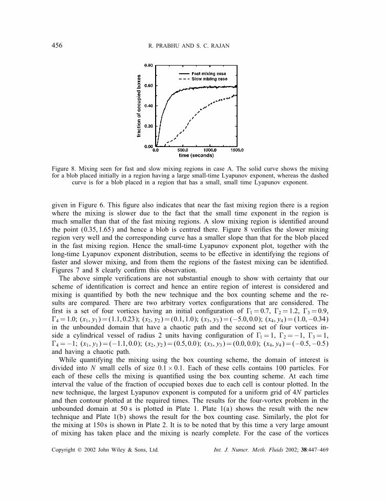
Figure 8. Mixing seen for fast and slow mixing regions in case A. The solid curve shows the mixingfor a blob placed initially in a region having a large small-time Lyapunov exponent, whereas the dashed

curve is for a blob placed in a region that has a small, small time Lyapunov exponent.

given in Figure 6. This &gure also indicates that near the fast mixing region there is a regionwhere the mixing is slower due to the fact that the small time exponent in the region ismuch smaller than that of the fast mixing regions. A slow mixing region is identi&ed aroundthe point (0:35; 1:65) and hence a blob is centred there. Figure 8 veri&es the slower mixingregion very well and the corresponding curve has a smaller slope than that for the blob placedin the fast mixing region. Hence the small-time Lyapunov exponent plot, together with thelong-time Lyapunov exponent distribution, seems to be e?ective in identifying the regions offaster and slower mixing, and from them the regions of the fastest mixing can be identi&ed.Figures 7 and 8 clearly con&rm this observation.The above simple veri&cations are not substantial enough to show with certainty that our

scheme of identi&cation is correct and hence an entire region of interest is considered andmixing is quanti&ed by both the new technique and the box counting scheme and the re-sults are compared. There are two arbitrary vortex con&gurations that are considered. The&rst is a set of four vortices having an initial con&guration of Q1 =0:7, Q2 =1:2, Q3 =0:9,Q4 =1:0; (x1; y1)= (1:1; 0:23); (x2; y2)= (0:1; 1:0); (x3; y3)= (−5:0; 0:0); (x4; y4)= (1:0;−0:34)in the unbounded domain that have a chaotic path and the second set of four vortices in-side a cylindrical vessel of radius 2 units having con&guration of Q1 =1, Q2 =−1, Q3 =1,Q4 =−1; (x1; y1)= (−1:1; 0:0); (x2; y2)= (0:5; 0:0); (x3; y3)= (0:0; 0:0); (x4; y4)= (−0:5;−0:5)and having a chaotic path.While quantifying the mixing using the box counting scheme, the domain of interest is

divided into N small cells of size 0:1× 0:1. Each of these cells contains 100 particles. Foreach of these cells the mixing is quanti&ed using the box counting scheme. At each timeinterval the value of the fraction of occupied boxes due to each cell is contour plotted. In thenew technique, the largest Lyapunov exponent is computed for a uniform grid of 4N particlesand then contour plotted at the required times. The results for the four-vortex problem in theunbounded domain at 50 s is plotted in Plate 1. Plate 1(a) shows the result with the newtechnique and Plate 1(b) shows the result for the box counting case. Similarly, the plot forthe mixing at 150s is shown in Plate 2. It is to be noted that by this time a very large amountof mixing has taken place and the mixing is nearly complete. For the case of the vortices



inside a circular cylinder the plots at 50 s are shown in Plate 3 and the plots for 150 s areshown is Plate 4. As can be clearly seen from the plots, apart from the di?erence in the actualnumerical values (and hence the colouring), which is only expected since one &gure gives theLyapunov exponent and the other gives the fraction of occupied boxes, that the agreement isexcellent. All the signi&cant features of importance, such as the relative regions of high andlow mixing, are very clearly identi&able from the contour plot of the Lyapunov exponent andthese match very well with the results obtained from the box counting technique.One of the main advantages of the present technique is that it is much more e:cient than

the box counting method both in terms of time taken as well as memory resources used forthe computation. This is clearly seen from the following discussion. For a small region ofsize 0:1× 0:1, 100 particles were advected in the box counting scheme, whereas only fourparticles were considered for the Lyapunov exponents. To compute the exponent at these fourpoints, eight particles are needed since the ghost particle technique is used. Hence this schemeis more e:cient by a factor of 12.5 both in terms of time and memory and yet e?ective inidenti&cation of the regions of fastest mixing.

7. BEHAVIOUR OF THE BLOB IN TIME

The evolution in time of a blob of tracer particles placed in either a chaotic or a regularregion for an initial vortex con&guration as in case A is studied. When the blob is placedin a chaotic region it mixes in the �uid and does not visit the regions where the motion isregular. This is seen in Figure 9.There are two types of regular behaviour that are observed. In the regular region near the

eye of the vortex, the blob stretches rapidly but the stretching is localized, i.e. it stretchesenormously but is con&ned in the vicinity of the vortex. This is seen in Figure 10. However,in the other regular regions that are not near the eyes of the vortices, the blob hardly stretchesand it more or less retains its shape (Figure 11).

8. RESULTS FOR OTHER INITIAL CONFIGURATIONS OF VORTICES

8.1. Integrable vortex motion

In this section the method described above is applied to other initial con&gurations of threeand four vortices that have integrable vortex motion.To begin with, the case of three vortices initially placed at the vertices of an equilateral

triangle of side 2 units is considered. The strength and position of the vortices are, respectively,Q1 =Q2 =Q3 =1:0; (x1; y1)= (−1; 0); (x2; y2)= (1; 0); (x3; y3)= (0;

√3). This is called case B.

For this case the vortices move on a circle centred at the centroid of the equilateral triangle.It is found that the exponent value is extremely small and that it decreases rapidly in time.This indicates that there is no positive Lyapunov exponent in such a �ow and that there isno possibility of mixing.The above initial con&guration of vortices is slightly perturbed resulting in an initial con-

&guration called case C and is given by Q1 =Q2 =Q3 =1:0; (x1; y1)= (−1; 0); (x2; y2)= (1; 0);(x3; y3)= (0; 1:6). For this case the Lyapunov exponent distribution is given in Figure 12. As



Figure 9. (a)–(e) show the evolution of a blob in time at 0, 50, 150, 300, 600s respectively for case A.The blob is placed in a region which is identi&ed as a chaotic and fast mixing one.

mentioned earlier, only the signi&cant contours are presented. It can be clearly seen that thereare large regions having a null Lyapunov exponent and small bands where it is positive. Henceit seems that, if the perturbation of the initial vortex positions is increased, larger regions ofchaotic tracer motion may be seen.



Figure 10. (a) and (b) show the development of a blob in time that is placed nearthe eye of a vortex (case A).

Figure 11. Plot showing the development of a blob placed in a regular region that is not near thevortices and is surrounded by regions of chaotic tracer motion (case A).

Earlier for case A, where three point vortices initially formed an isosceles triangle, it wasseen that there were regular regions near the eyes of the vortices. Other regions of regularmotion were also identi&ed and were given in Figure 3. This con&guration of vortices issigni&cantly di?erent from case B (vortices placed on an equilateral triangle), where theentire region has regular motion. Hence, from the results of cases A and C, it seems that asthe circular motion of the vortices is slowly perturbed, the regular regions gradually break upinto distinct regions having either regular or chaotic motion.In order to check this, the con&guration of the three vortices is made asymmetric by

choosing the initial co-ordinates as (x1; y1)= (−1; 0); (x2; y2)= (1; 0); (x3; y3)= (0:5; 0:75)and choosing Q1 =Q2 =Q3 =1:0. This is called case D and its Lyapunov exponent distributionis given in Figure 13. For this case it is clearly seen that there are about four regular regionsapart from the ones near the eyes of the vortices but these are very small in size comparedto those seen in Figure 3 (case A).



Figure 12. Contour plot of the Lyapunov exponent distribution for case C and for a tmax of 20 000 s.The solid line is a contour of 0.01 and the dashed line is a 0.001 contour.

Figure 13. Contour plot of the Lyapunov exponent distribution for case D and for a tmax of 20 000 s.The solid line is a contour of 0.018 and the dashed line is a 0.003 contour.

The initial con&guration of case D is further altered by making it more asymmetric. The cho-sen initial con&guration is Q1 =Q2 =Q3 =1:0; (x1; y1)= (−1; 0); (x2; y2)= (1; 0); (x3; y3)= (1; 1).This case is called case E and the Lyapunov exponent distribution is given in Figure 14. Itcan be seen that there is only one regular region of motion apart from the ones near the eyesof the vortices and this also is very small. This indicates that in order to have large regionsin the �ow where the tracer motion is chaotic, the initial vortex con&guration of case B mustbe altered signi&cantly.Three vortices on a line are considered next and this is called case F. The initial con&gu-

ration of the vortices is Q1 =Q2 =Q3 =1:0; (x1; y1)= (−1; 0); (x2; y2)= (0; 0); (x3; y3)= (1; 0).



Figure 14. Contour plot of the Lyapunov exponent distribution for case E and for a tmax of 20 000 s.The solid line is a contour of 0.015 and the dashed line is a 0.003 contour.

Figure 15. Contour plot of the Lyapunov exponent distribution for case G and for a tmax of 20 000 s.The solid line is a contour of 0.02 and the dashed line is a 0.004 contour.

For this con&guration the vortices at the ends of the line move on a circle and for all thetracer particles the Lyapunov exponent is zero. Case F is perturbed slightly resulting incase G and for this the initial con&guration of vortices is Q1 =Q2 =Q3 =1:0; (x1; y1)= (−1; 0);(x2; y2)= (0; 0:05); (x3; y3)= (1; 0). The corresponding Lyapunov exponent distribution isgiven in Figure 15. As seen clearly, there are a few small regular regions of motion apartfrom the ones near the eyes of the vortices. This is signi&cantly di?erent from the earlier caseC, which is a slightly perturbed version of case B (vortices on an equilateral triangle). CaseF is di?erent from case B because it is unstable. This instability leads to a vortex motion thatis signi&cantly di?erent from a circular one even when slightly perturbed.Case H, of four vortices which move in a circle having initial con&guration as Q1 =Q2 =

Q3 =Q4 =1:0; (x1; y1)= (−1; 0); (x2; y2)= (1; 0); (x3; y3)= (0; 1); (x4; y4)= (0;−1) isalso considered. Here too there are no regions where a positive Lyapunov exponent is seen.This case is similar to case B, wherein there is no chaotic tracer motion anywhere in the�ow.



Figure 16. Contour plot of the Lyapunov exponent distribution for case I and for a tmax of 20 000 s.The solid line is a contour of 0.012 and the dashed line is a 0.002 contour.

Figure 17. Contour plot of the Lyapunov exponent distribution for case J and for a tmax of 20 000 s.The solid line is a contour of 0.02 and the dashed line is a 0.005 contour.

The above con&guration is perturbed by a small amount resulting in case I, givenas Q1 =Q2 =Q3 =Q4 =1:0; (x1; y1)= (−1; 0); (x2; y2)= (1; 0); (x3; y3)= (0; 0:9); (x4; y4)=(0;−1). The Lyapunov exponent distribution for this is given in Figure 16. It is seen that thereare large regions of regularity and small bands where there is a positive Lyapunov exponent.This is similar to that seen in Figure 12 for the corresponding three vortex problem (case C).Hence, it is seen that upon perturbing the circular orbits of the vortices, regions of chaotictracer motion gradually appear.Another case of four vortices is considered for which the initial vortex con&guration is given

by Q1 =Q2 =Q3 =Q4 =1:0; (x1; y1)= (−1; 0); (x2; y2)= (1; 0); (x3; y3)= (0; 1); (x4; y4)= (0; 0).This is called case J and the exponent distribution for it is as given in Figure 17 and indicatesthat there is a small regular region near the boundary. This is similar to the earlier case E, inthat the vortex con&guration is greatly altered from that of its corresponding circular motion(case G).All the above observations are made by studying the Lyapunov exponent plot at large times.

For the asymmetric initial con&guration of three vortices given earlier as case D, the small



Figure 18. Mixing for fast and slow mixing regions in case D. The blobsconsidered have 6561 particles in them.

time exponent plot is studied and a slow mixing region is identi&ed. This slow mixing regionis centred around the point (0:1; 0:15). A blob, initially having a dimension of 0:1× 0:1 andhaving 6561 particles in it, is centred at this point and the mixing of the blob is quanti&edas mentioned in an earlier section. Similarly a fast mixing region is identi&ed and is centredat the point (0.825, 1.5). A blob having the same properties is chosen for this case also. Themixing for both the fast and slow mixing regions are plotted in Figure 18. It can be seen thatthe blob placed initially in the fast mixing region mixes more quickly than the correspondingone in the slow mixing region. The present slow mixing is faster than that of the earlier caseviz. Figure 8. It is to be noted that in the case of Figure 8, the slow mixing is very poor inthe sense that the blob did not start stretching until after a very long time and even then therate is much slower than the corresponding fast mixing case presented in Figure 18.Similar to the �ow in the unbounded domain, the �ow of three vortices inside a cylinder

was also considered and very similar results were obtained. Here too as the motion of thevortices was perturbed from circular motion, regions of chaotic tracer motion appeared andas the perturbation increased, the size of the regular regions slowly reduced just as observedabove. However, these results are not presented.In order to understand the behaviour of the Lyapunov exponent in time for the earlier

mentioned integrable four-vortex motion (case J), the Lyapunov exponent for a few tracerparticles is plotted with respect to time and is given in Figure 19. The plot clearly indicates thatthere are two types of behaviour of the Lyapunov exponents. One which rapidly converges tozero and the other which converges to a &xed positive value. All the chaotic orbits consideredappear to have the same Lyapunov exponent. In order to check this for larger computationaltimes, the computations for two of the chaotic orbits are done for a time of 106 natural timeunits and are plotted in Figure 20. It can be seen that they converge to one positive value.

8.2. Chaotic vortex motion

In this section, the results of various computations are presented for a chaoticfour-vortex problem, having an initial vortex con&guration given by Q1 =Q2 =Q3 =Q4 =1:0;(x1; y1)= (−1; 0); (x2; y2)= (1; 0); (x3; y3)= (0; 1); (x4; y4)= (0; 0:4). This is called case K.



Figure 19. Plot of the Lyapunov exponent with time for the integrable vortexmotion (case J). tmax is 100 000 s.

Figure 20. A plot of the Lyapunov exponent (case J) with time for twochaotic orbits. tmax is 100 0000 s.

In Figure 21 the behaviour of the Lyapunov exponent in time for the chaotic four-vortexmotion (case K) is plotted for a few di?erent initial conditions of tracer particles. It is seenthat for one of the initial conditions the exponent rapidly converges to zero. This point is veryfar away from the vortices and hence its behaviour is regular. The other ones are closer to thevortices and a few appear to converge to one exponent value while a few others do not seemto do so, unlike the behaviour seen in the integrable case. In order to see if there is really aconvergence to any value, the computation is again performed for a time of 106 s and as canbe seen in Figure 22 the values do not converge and continue to change. This is in sharpcontrast to what was seen earlier for the integrable vortex motion given in Figures 19 and 20.In order to con&rm this observation, further computations are performed for a set of about 60initial tracer locations having chaotic motion. For this set of particles, the Lyapunov exponentis computed for both the integrable vortex motion (case J) and the chaotic vortex motion(case K). The standard deviation divided by the mean of the Lyapunov exponent for variouschaotic vortex motion cases and various non-chaotic vortex motion cases are computed andplotted as a function of time in Figure 23. It is seen that the value decreases and is much



Figure 21. Plot of the Lyapunov exponent with time for the chaotic vortexmotion (case K). tmax is 100 000 s.

Figure 22. Plot of the Lyapunov exponent (case K) with time for two chaotic orbits. tmax is 100 0000 s.

less for integrable case, whereas for the chaotic case it is much higher—almost by a factorof three. However, when the exponents for the chaotic vortex motion inside a cylinder areconsidered such results are not seen. In Figure 24 the standard deviation divided by meanis plotted both for chaotic and regular vortex motion for a collection of about 60 particleseach. It can be clearly seen that the standard deviation of the exponent is small comparedwith the mean, hence it appears that the Lyapunov exponents converge just as in the regularunbounded vortex motion case. For the unbounded chaotic vortex motion, computations for asmaller number of particles using smaller eps values were performed but they revealed similarresults.The Lyapunov exponent distribution for the chaotic four vortex problem (case K) is plotted

in Figure 25. The regions near the eye of the vortices continue to show a regular motion.Apart from this there are several small regions where the exponents appear to be small. Fromthe earlier plots for the convergence of the exponent it is seen that these values are notindicative of regular motion. Also from the earlier discussion of integrable vortex motion itis seen that as the initial con&guration is changed from that which produces circular vortexmotion, the regular regions reduce in size and ultimately such regions become negligibly small.



Figure 23. Plot of the standard deviation of the Lyapunov exponents divided by the mean for varioustracer particles in an unbounded �ow for various intial vortex con&gurations. The solid lines are forvortex con&gurations that undergo chaotic motion and the dotted lines are for regular vortex motion.

Figure 24. Plot of the standard deviation of the Lyapunov exponents divided by the mean for var-ious tracer particles inside a circle for various initial vortex con&gurations. The solid lines are forvortex con&gurations that undergo chaotic motion and the dotted lines are for regular vortex motion.

In order to have a chaotic vortex motion the initial vortex con&guration must be changed quitedrastically from that which produces circular vortex motion viz. case H. This is seen in thecon&guration of vortices chosen in case K. This suggests that there should be no regularregion apart from the ones near the eye of the vortices and the region far away from thevortices. This has been veri&ed by studying the development of a blob of tracer particles intime. However, the results are not presented here. Hence, for a velocity &eld that displaysEulerian chaos it appears that there are no regular regions apart from the ones near the eyesof the vortices and the one that is very far away.The small-time Lyapunov exponent distribution for the chaotic four-vortex problem is plot-

ted for two di?erent eps values of 10−7 and 10−8. Each computation is done with a di?erentset of random angles. It is found that the plots are very similar. From the plots, two sam-ple regions of fast and slow mixing are identi&ed to be initially centred at (1:25;−0:5) and



Figure 25. Contour plot of the Lyapunov exponent distribution for case K and for a tmax of 20 000 s.The solid line is a 0.02 contour and the dashed line is a 0.006 contour.

Figure 26. Mixing rates for blobs placed in fast and slow regions of mixing for thechaotic four-vortex problem (case K).

(−0:55; 0:85) respectively. As is done in the previous section, the mixing of a blob in thoseregions is quanti&ed by the box counting scheme. The results are presented in Figure 26. Ascan be seen, the blob placed in the fast mixing region starts mixing immediately and hencemakes the mixing e:cient there. Hence, in-spite of the fact that the Lyapunov exponent doesnot converge in time, the method described in this paper is successful in the identi&cation ofthe regions of fastest and most e:cient mixing.

9. CONCLUSIONS

The observations made in the previous sections indicate that in the regions near the eye of thevortices and the regions far away from the vortices, the tracer particles exhibit regular, non-chaotic motion irrespective of the nature of the vortex motion (regular or chaotic). This result



is consistent with that obtained by Babiano et al. [6]. However, the method described in thispaper has identi&ed other regions of regular motion. It is also observed that only signi&cantlylarge changes of the initial con&guration of vortices from the one which produces a circularvortex motion leads to the creation of large regions of chaotic tracer motion. Hence, it canbe stated that there is a strong connection between the vortex motion and the regions ofregularity that are not near the eye of the vortices.It has also been shown in this paper that from the knowledge of the small-time Lyapunov

exponent distribution, the regions of most e:cient mixing for a given initial con&gurationof vortices can be identi&ed. This technique is also shown to be accurate and much moree:cient than the traditional box counting scheme.From the computations presented in this paper it is seen that for a chaotic four-vortex motion

in the unbounded domain, the Lagrangian Lyapunov exponent does not converge properly.For integrable vortex motion, the exponent is shown to converge. It has also been shown thatfor chaotic vortex motion inside a cylinder, the Lyapunov exponent converges. Hence, caremust be taken while interpreting long-time Lyapunov exponent values for unbounded chaoticvortex motion cases. At this juncture it is not possible to say if the non-convergence is dueto numerical error or due to a more fundamental problem.The procedure used to identify the regions of highest mixing is general and can also be

applied to other �ows (including three-dimensional �ows) so long as the trajectory of theparticle can be computed. Hence, the regions of most e:cient mixing can be identi&ed bystudying the distribution of the largest Lagrangian Lyapunov exponent for large and smalltimes. Thus, the present method of identi&cation of regions of fast mixing appears to bepromising.

ACKNOWLEDGEMENTS

Most of the computations were performed at the computational facility of the Department of Aero-space Engineering, IIT Madras. The authors wish to thank Dr P. Sriram and Dr M. Ramakrishna,Associate Professors, Department of Aerospace Engineering, IIT Madras, for their help and guidance.They also wish to thank Dr Neelima Gupte, Assistant Professor, Department of Physics, IIT Madras forher useful suggestions; express their gratitude to S. Shashidhar, MS Scholar, Department of AerospaceEngineering, IIT Madras (presently with Flow Consultants, Pune, India) for his help in the preparationof this article.

REFERENCES

1. Ottino JM. The Kinematics of Mixing: Stretching, Chaos, and Transport. Cambridge University Press:Cambridge, 1989.

2. Novikov EA. Dynamics and statistics of a system of vortices. Soviet Physics JETP 1984; 41:937.3. Aref H. Motion of three vortices. Physics of Fluids 1979; 22(3):393.4. Aref H, Pomphrey N. Integrable and chaotic motions of four vortices. Physics Letters 1980; 78A(4):297.5. Aref H, Pomphrey N. Integrable and chaotic motions of four vortices I—the case of identical vortices.

Proceedings of the Royal Society London Series A 1982; 380:359.6. Babiano A, Bofetta G, Provenzale A, Vulpiani A. Chaotic advection in point vortex models and two-dimensional

turbulence. Physics of Fluids 1994; 6(7):2465.7. Aref H. Stirring by chaotic advection. Journal of Fluid Mechanics 1984; 143:1.8. Franjione JG, Ottino JM. Feasibility of numerical tracking of material lines and surfaces in chaotic �ows.

Physics of Fluids 1987; 30:3641.9. Aref H. Integrable, chaotic, and turbulent vortex motion in two dimensional �ows. Annual Review in Fluid

Mechanics 1983; 15:345.



10. Prabhu R. Chaos and mixing in vortex dominated �ows. Bachelor of Technology Thesis, Indian Institute ofTechnology Madras, 1997.

11. Press WH, Teukolsky SA, Vetterling WT, Flannery BP. Numerical Recipes in ‘C’. Cambridge University Press:Cambridge, 1992.

12. Peitgens HO, Jurgens H, Saupe D. Chaos and Fractals, New Frontiers of Science. Springer: New York, 1992.


Documents

Identification of regions of fastest mixing in a system of point vortices