Embed Size (px)
Citation preview
JOURNAL OF MATHEMATICAL ANALYSIS AND APPLICATIONS 14, 275-303 (1989)
Identification of Flexural Rigidity in a Dynamic Plate Model*
L. W. WHITE
Department of Mathematics, University of Oklahoma, Norman, Oklahoma 73019
Submitted by V. Lakshmikantham
Received October 9, 1987
The estimation of spatially dependent flexural rigidity coefficients in Kirchhoff models is discussed using an output least-squares method in H* regularization. The regularity of optimal estimators is studied and these properties are used to develop an approximation theory. Several numerical examples are presented. 0 1989
Academic Press, Inc.
0. INTRODUCTION
In this note we study the estimation of elastic parameters within dynamic linear Kirchhoff plate models. That is, given data z in an observation space 2 we seek a parameter a, from within an admissible set of parameters Qad such that the solution of the resulting plate equation gives rise to an observation “matching” z. We assume that no damping is present so that in fact our formulation is independent of damping. More precisely, let 52 be an open bounded domain in R* with boundary r that is at least Lipschitz. We consider the equation
u,,+Au=f in Qx (0, T) (O-1 1
with initial conditions
u(0) = uo
u,(O) = u1,
where A is a fourth order elliptic operator given by
(0.2)
Au = d(adu) (0.3)
* This work was partially supported by AFOSR Grant AFOSR-84-0271.
275 0022-247X/89 $3.00
Copyright 0 1989 by Academic Press, Inc. All rights of reproduction in any form reserved.
276 L. W. WHITE
Au=~~u~u)+ (1 -o)((wqx,),,.q
+ (UUr2xJx2.x2 + 2(%,x,L,xJ. (0.4)
The operators A are accompanied with boundary conditions that we assume for the most part to represent clamped boundary conditions
u2d-j dn
on r. (0.5)
or simply supported conditions
u=u x,.x, = U x,x* = U x2 12 =o on r. (0.6)
In Eq. (0.4), cr is called Poisson’s coefficient, 0 <g < f. The parameter a = a(x) in (0.3) and (0.4) is called the flexural rigidity and depends on the material properties of the plate: Young’s modulus and Poisson coefficient, as well as the thickness of the plate, [20]. For constant a, Eq. (0.4) becomes Eq. (0.3). If a is a function of position, the model (0.3) takes into account moments parallel to the x- and y-axes with no twisting while (0.4) accomodates twisting moments as well [20]. While parameter estimation in beams has been investigated, e.g., [4-6, lo], relatively little has been done for plates.
Of interest in this note is the estimation of a by means of regularized output least-squares method. The regularization is through the inclusion of an H2-norm term. This space is used since it is natural in the sense that it is the smallest integer Sobolev space imbedding into L”(Q) where 52 c R2. The regularization technique is studied in [12] as a way to stablize least- square estimation. There, under certain identifiability assumptions, it is demonstrated that for certain regularizations the optimal regularized least- squares estimators are stable with respect to data. In other works it is shown for other equations [ 11,211 that these solutions may exhibit additional regularity than is even assumed in the regularization.
In this work we formulate several estimation problems based upon observation of displacements and velocities. We show that for (0.1) with A given by (0.3) there are certain natural conditions for identifiability. Hence, the stability results of [ 123 hold. If there actually exists a least-square optimal estimator, we show that the regularized estimators converge to it as the regularization parameter goes to zero. For this equation we observe that further conditions are required on the data and the solution of the equation itself in order to characterize the optimal estimators as solutions of a system of Euler equations. By means of the Kuhn-Tucker Theorem we may deduce regularity of the optimal estimator. These regularity properties
IDENTIFICATION OF FLEXIJRAL RIGIDITY 277
are useful in formulating estimation problems for semidiscrete Galerkin approximating systems of initial value problems and investigating their limiting behavior. We find roughly speaking that for a regularized problem every weak H2 limit of the sequence of solutions of the discrete problems is a solution of the regularized output least-square problem.
1. FORMULATION OF ESTIMATION PROBLEMS
Let Vc H be Hilbert spaces such that V is dence in H and the imbed- ding of V into H is compact. Let Q be a bounded open domain in iR2 with a Lipschitz boundary r so that we may integrate by parts, [9]. We take
H = L2(f2)
and
0) V= H,$?) (1.1)
or
(ii) V= H;(Q) n H’(Q).
Let a( ., .): V x V + R be a continuous coercive symmetric bilinear form on V. That is, there exist positive constants C, and vA such that for any cp, I++ in V
b(cp, 11/l G CA II44 Y IIIc/II Y (1.2)
at% q) a vA IIdI;. (1.3)
Remark 1.1. In the case of a thin plate occupying the domain Q, the bilinear form is associated with operators of the type (0.2) or (0.4) with
4~ $I= j 0) h(x) Mx) dx (1.4) R
or
+ (ox&) +x&) + 2rpx,xz(x) ll/x,x,(x))l dx. (1.5)
We assume that the function a(x) satisfies
aEL”(M),a(x)~v>o a.e. in Sz. (1.6)
For V satisfying (1.1)(i) or (ii) the bilinear forms specified in (1.4) and (1.5) satisfy (1.2) and (1.3) [ 133.
409/144/l-19
278 L. W. WHITE
The bilinar form a( . , .) determines a continuous linear operator d: V+ V’ by
4% II/)= Cd% $ > for cp, $ in V. (1.7)
Moreover, defining the set
D(A)= {UE v: dz4EH)
we may define the linear operator A: D(A) -+ H by Au = du for u E D(A ) and note that if u E D(A) then
a(u, u) = (Au, II)
and the mapping of V into R
u I-+ a(u, u)
is continuous with respect to the H-topology. The operator A is positive definite, self-adjoint and unbounded. It is well-known that fractional powers of A are defined and that V = D(A ‘I*), [ 141.
Under the above assumptions on a( ., .), it follows that given fe F” there exists a unique u E V such that
for every cp E V and
4u,cp)=(.Lcp) (1.8)
II4 “G C(a) llfll y’? (1.9)
where for a( ., .) as in Remark 1.1 the mapping takes bounded sets in L”(Q) satisfying (1.6) to bounded sets in lR+, [7].
To give regularity theorems cf [2] for (1.8) we make the assumption
r is C4. (1.10)
Since HP(D) imbeds continuously into C’(D) for p > 2, [l] the following results hold.
PROPOSITION 1.1. Letf~ L2(Q), (1.1)(i), (1.4~(1.6), and (1.10) hold. Zf a E H2+y(G?) with y > 0, then
and
D(A) c H;(Q) n H3(Q)
Ilull f&q G C(a) llSllL+2,%
IDENTIFICATION OF FLEXURAL RIGIDITY 279
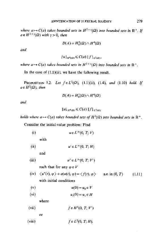
where a H C(a) takes bounded sets in H2+y(SZ) into bounded sets in R+. Zf a E H3+Y(Q) with y > 0, then
D(A) = H&Q) n H4(Q)
and
Ilull H4(n) G C(a) Ilf II L2cQj,
where a H C(a) takes bounded sets in H3+y(B) into bounded sets in R+.
In the case of (l.l)(ii), we have the following result.
PROPOSITION 1.2. Let f EL2(f2), (l.l)(ii), (1.4), and (1.10) hold. If a E H’(Q), then
D(A) = H,‘(Q) n H4(f2)
and
Ilull H4(o) G C(a) Ml L2(n)
holds where a H C(a) takes bounded sets of H2(Q) into bounded sets in R +.
Consider the initial-value problem: Find
0) UEL”(0, T; V)
with
(ii) U’E L”(0, T; H)
and
(iii) U”E L”(0, T; v’)
such that for any rp E V
(iv) (u”(t), cp> + 44th cp) = (f(t), rp> a.e. in (0, T) (1.11)
with initial conditions
(VI u(O)=u,E v
(vi) u,(O) = u1 E H
where
(vii) f E H’(0, T; V’)
or
(viii) f~ L’(O, T; H).
280 L. W. WHITE
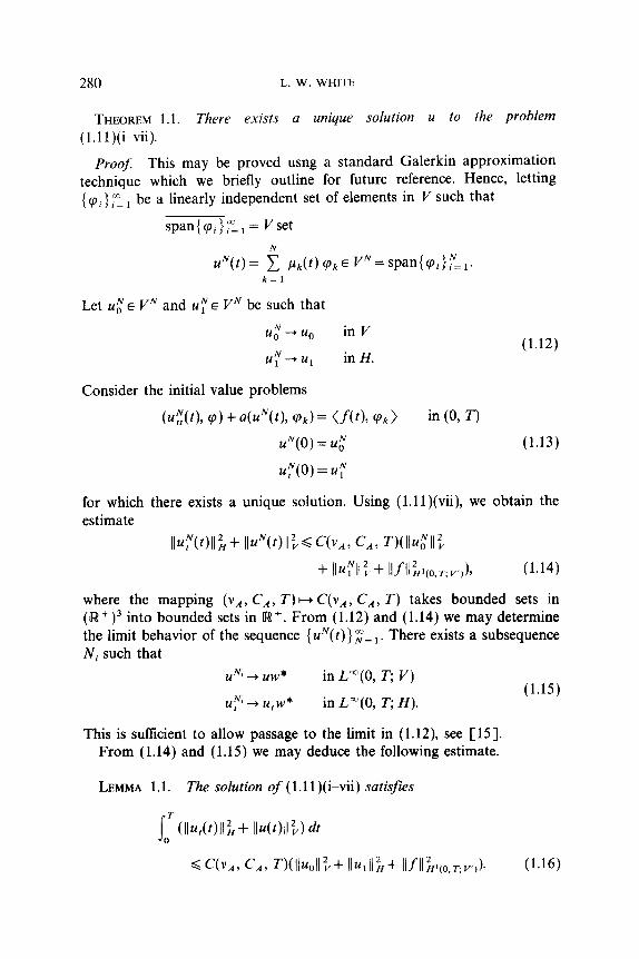
THEOREM 1.1. There exists a unique solution u to the problem ( 1. 1 1 )( i-vii).
Proof: This may be proved usng a standard Galerkin approximation technique which we briefly outline for future reference. Hence, letting (cp,} E r be a linearly independent set of elements in V such that
span{cpi)p”_, = I/set
UN(t)= $ pk(t)(PkE VN=Span{cpi}~zl. k=l
Let ut E VN and uy E VN be such that
u+40 in V
U;y-+U1 in H. (1.12)
Consider the initial value problems
(uz(t)y v) + a(uN(th (Pk)= <ftth vk) in (0, T)
UN(O) = uo” (1.13)
u;(o) = u;”
for which there exists a unique solution. Using (l.ll)(vii), we obtain the estimate
ll~;“ONl~+ Ilu”O)ll:~W,, C/i, T)(llu,NIIt
+ b3l’, + IISII f&I, T; V’,)> (1.14)
where the mapping (vA, C, , T) H C(v, , C, , T) takes bounded sets in (R’)3 into bounded sets in R +. From (1.12) and (1.14) we may determine the limit behavior of the sequence {u”(t)} z= r. There exists a subsequence Ni such that
UN, -+ uw* in L”(0, T, V)
U;” -+U,W* in L”(0, T; H).
This is sufficient to allow passage to the limit in (1.12), see [ 151. From (1.14) and (1.15) we may deduce the following estimate.
LEMMA 1.1. The solution of (1.11 )(i-vii) satisfies
f o~(ll~,(~Nl:I+ IIWI:) dt
(1.15)
d C(v,, CA, ~~woll:+ ll~,llz,+ IIfII2Hl@,T;Y’)). (1.16)
IDENTIFICATION OF FLEXURAL RIGIDITY 281
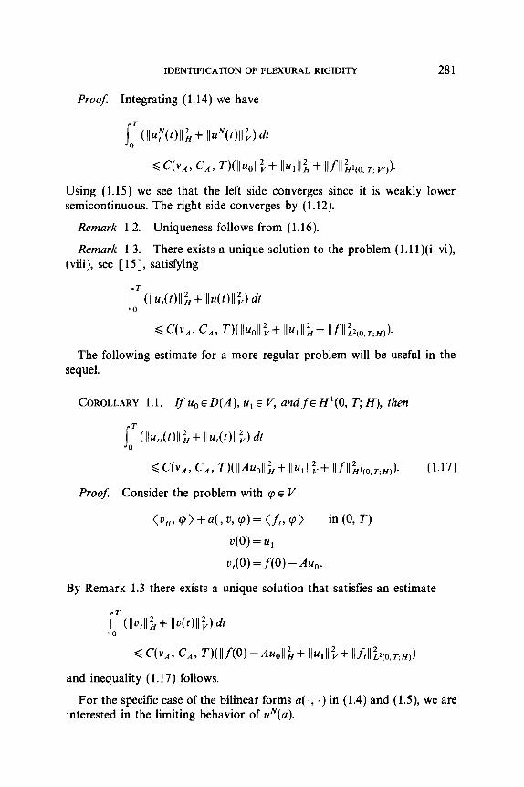
Proof Integrating (1.14) we have
I o=W’(N:+ b”b)ll;) dt G C(v,, c.4, n~Il~oll:f Il%ll;+ llfllffl(o,T; V’,).
Using (1.15) we see that the left side converges since it is weakly lower semicontinuous. The right side converges by (1.12).
Remark 1.2. Uniqueness follows from (1.16).
Remark 1.3. There exists a unique solution to the problem (1.1 l)(i-vi), (viii), see [ 151, satisfying
s oT(Ilu,Wll~+ Il4t)ll;W
GC(v,, c,, nIl~,ll;+ lblII:,+ IlfIIt~(0,T;H))’
The following estimate for a more regular problem will be useful in the sequel.
COROLLARY 1.1. If u0 ED(A), u1 E V, andfE H’(0, T; H), then
s o=(ll~ttO)ll~+ Ilu&llt)dt
6 ‘3v,> CA, T)(Il-hll;+ lM;+ llfll;~~o,T;~~). (1.17)
Proof Consider the problem with cp E V
<utt, cP)+4, u, rp)= cfr~ cp> in (0, T)
u(0) = 241
u,(O) =f(O) - Au,.
By Remark 1.3 there exists a unique solution that satisfies an estimate
s TW41ir+ IlWl;)dt
0
G C(v,, c,, ~W(O)-~~oll:,+ llulllz+ llfrlltqo,r;H,)
and inequality (1.17) follows.
For the specific case of the bilinear forms a( ., .) in (1.4) and (1.5), we are interested in the limiting behavior of u”(u).
282 L. W. WHITE
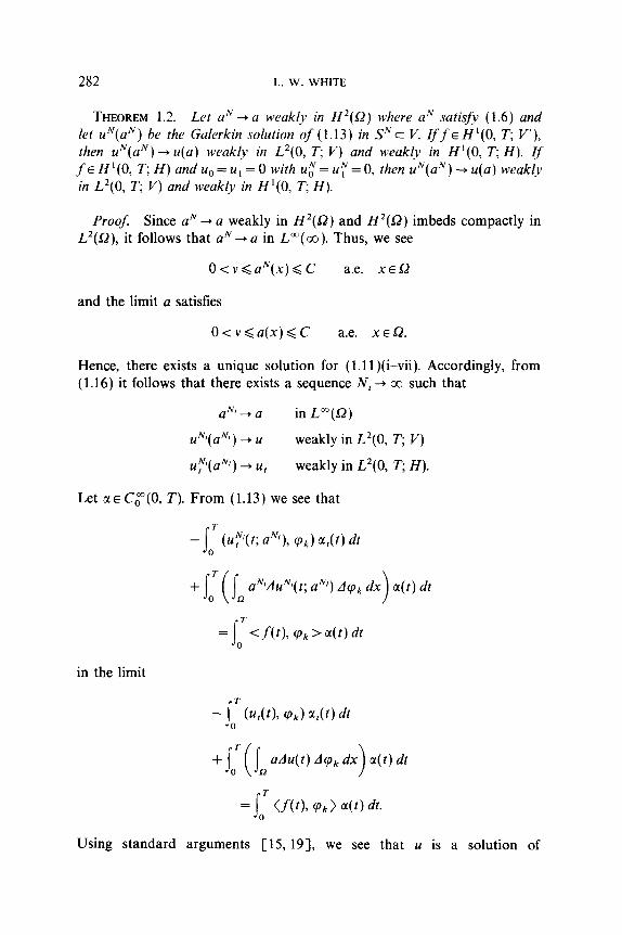
THEOREM 1.2. Let aN + a weakly in H2(Q) where aN satisfy (1.6) and let u”(a”) be the Galerkin solution of (1.13) in SNc I/. Iff eH'(0, c V'), then u”(a”) --) u(a) weakly in L2(0, T; V) and weakly in H’(0, T; H). Zf f E H’(0, T; H) and u0 = u, = 0 with ~40” = u;” = 0, then u”(a”) --) u(a) weakly in L2(0, T; V) and weakly in H’(0, T; H).
Proof: Since aN -P a weakly in H2(Q) and H’(Q) imbeds compactly in L2(0), it follows that aN -+ a in L”(m). Thus, we see
O<v<aN(x)<C a.e. xEQ
and the limit a satisfies
0 -c v < a(x) < C a.e. x E 52.
Hence, there exists a unique solution for (l.ll)(i-vii). Accordingly, from (1.16) it follows that there exists a sequence IV,--+ cc such that
aNf-ia in L”(Q)
uNl(aN’) -+ 24 weakly in L’(O, T, V)
uy(a”) + u, weakly in L2(0, T; H).
Let tl~ C,“(O, T). From (1.13) we see that
- s or (u;“‘(t; aNO, (~~1 a,(f) dt + joT ( L aN’AuN’(t; aN’) Acp, dx
> a(t) dt
I
r = <f(t), (Pk'dt) df
0
in the limit
(Pk) a,(t) dt
+ JOT ( L aAu(t) Acp, dx >
a(r) dt
= <f(t), (Pk > a(t) dl.
Using standard arguments [15, 191, we see that u is a solution of
IDENTIFICATION OF FLEXURAL RIGIDITY 283
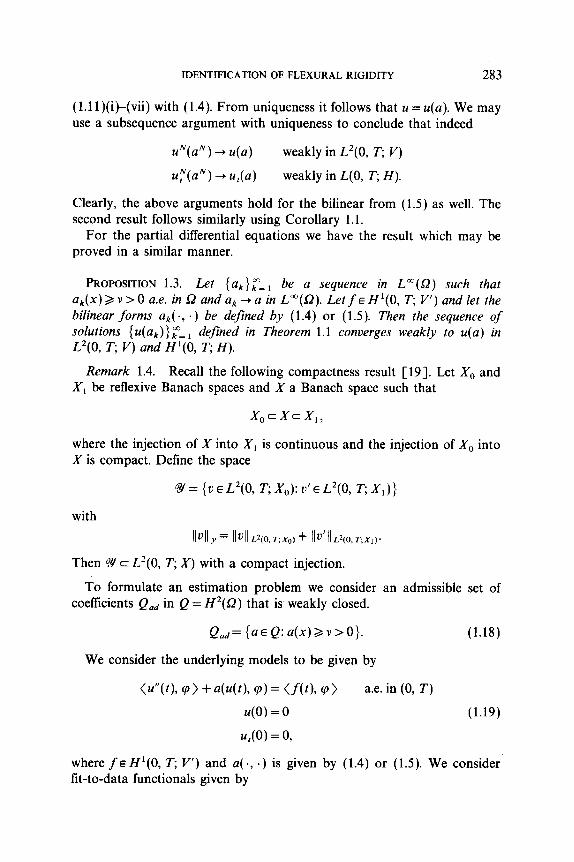
(1.11)(i)-(vii) with (1.4). From uniqueness it follows that u = u(a). We may use a subsequence argument with uniqueness to conclude that indeed
u”(a”) + u(u) weakly in L2(0, T; V)
~;“(~“) + u,(a) weakly in L(0, T; H).
Clearly, the above arguments hold for the bilinear from (1.5) as well. The second result follows similarly using Corollary 1.1.
For the partial differential equations we have the result which may be proved in a similar manner.
PROPOSITION 1.3. Let {u~}~=~ be a sequence in L”(O) such that uk(x) 2 v > 0 u.e. in Q and uk + a in L”(Q). Let f E H’(0, T, V’) and let the bilinear forms uk( -, . ) be defined by (1.4) or (1.5). Then the sequence of sohtions { u(ak)}km_ 1 d f e me in Theorem 1.1 converges weakly to u(u) in d L2(0, T; V) and H’(0, T; H).
Remark 1.4. Recall the following compactness result [19]. Let X0 and X, be reflexive Banach spaces and X a Banach space such that
where the injection of X into X, is continuous and the injection of X,, into X is compact. Define the space
+Y={vEL2(0, T&):v’EL2(0, T;X,)}
with Ml, = Il4lrq,,T;&) + Ilu’llLqcl P,yI)’ . .
Then Y c L2(0, r; X) with a compact injection.
To formulate an estimation problem we consider an admissible set of coefficients Qad in Q = H2(&!) that is weakly closed.
Qad= (u~Q:u(x)2v>O}. (1.18)
We consider the underlying models to be given by
(u”(t), rp> + 44th cp) = (f(t), cp> a.e. in (0, T)
u(0) = 0 (1.19)
u,(O) = 0,
where f E H’(0, T; V’) and a(., .) is given by (1.4) or (1.5). We consider fit-to-data functionals given by
284 L. W. WHITE
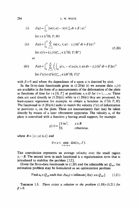
6) J(q)=SIllu(r;a)-z(t)ll:,dt+P ll42 0
for z E L’(O, T; H)
(ii) J(Q)= JOT,! (U(Xi, t;a)-Zj(t))‘dt+b IlUll
l-1 (1.20) for z(t) = (z,(t));=, EL’(O, T; Rw)
or
(iii) x(xi-xx) ut(x, t; a) d~-i~(t))~ dt+j? Ilal12
for i’(t)e (ii(t)):= i E (H’(0, T))”
with /? > 0 and where the dependence of u upon a is denoted by u(a). In the fit-to-data functionals given in (1.2O)(i-ii) we assume data z,(t)
are available in the form of o measurements of the deformation of the plate as functions of time for t E [0, T] at positions xi E 52 for i = 1, . . . . w. These data are used directly in (1.2O)(ii) while in (1.20)(i) they are processed, by least-square regression for example, to obtain a function in L2(0, T; H). The functional in (1.2O)(iii) seeks to match the velocity ii(t) of deformation at positions xi on the plate. These are measurements that may be taken directly by means of a laser vibrometer apparatus. The velocity U, of the plate is convolved with a function x having small support, for example
XGB otherwise,
where B= {x: 1x1 GE} and
0 < E < 1 mj;, dist(x,, r). . .
This convolution represents an average velocity over the small region xi - B. The second term in each functional is a regularization term that is introduced to stabilize the problem [12].
Given the lit-to-data functionals in (1.20) and the admissible set Qadd, the estimation problem may be formulated as an optimization problem
Find a, E Qad such that J(a,) = infimum{J(a): a E Q,,}. (1.21)
THEOREM 1.3. There exists a solution to the problem (1.18)-(1.21) for /I > 0.
IDENTIFICATION OF FLEXURAL RIGIDITY 285
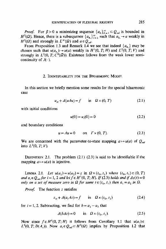
Proof: For p > 0 a minimizing sequence { uk}p=, c Qd is bounded in H’(G). Hence, there is a subsequence {L+.,}~, such that ak, + a weakly in H2(sZ) and strongly in L”(Q) and UE Qad.
From Proposition 1.3 and Remark 1.4 we see that indeed {ak,} may be chosen such that u(a,J --) u(a) weakly in H’(0, T; H) and L’(O, T, V) and strongly in L’(O, r; C’(D)). Existence follows from the weak lower semi- continuity of J(. ).
2. IDENTIFIABILITY FOR THE BIHARMONIC MODEL
In this section we briefly mention some results for the special biharmonic case
u,, + d(aAu) =f in L?x (0, T) (2.1)
with initial conditions
u(0) = u,(O) = 0 (2.2)
and boundary conditions
u=Au=O on TX (0, T). (2.3)
We are concerned with the parameter-to-state mapping a c, u(a) of &, into L2(0, T; V).
DEFINITION 2.1. The problem (2.1 k(2.3) is said to be identifiable if the mapping a H u(a) is injective.
LEMMA 2.1. Let ~(a,)= u(a,)=z in L2 x (to, tl) where (to, t,)c (0, T) and ai E Q,, for i = 1, 2 and let f E H’(0, T; H). If (2.3) holds and ifAz(t) = 0 only on a set of measure zero in D for some t E (to, tl) then a, = a2 in 0.
Proof The function z satisfies
Z,, + A(aiAz)=f in Sz x (to, t,) (2.4)
for i = 1,2. Subtracting, we find for b = a, -a, that
A(bAz) = 0 in Sz x (to, tl). (2.5)
Now since f E H’(0, T; H) it follows from Corollary 1.1 that u(a,)E L2(0, T; D(Ai)). Now uic Qadc H’(a) implies by Proposition 1.2 that
286 L. W. WHITE
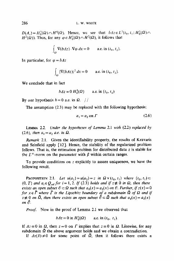
D(Ai) = HA(Q) n H4(52). Hence, we see that bdz E L2(t,, t,; Hi(Q) n H’(Q)). Thus, for any q E Hi(Q) n H’(Q), it follows that
s V( bdz) . Vq dx = 0 a.e. in (to, ti). R
In particular, for cp = bAz
I IV(bdz)J2 dx=O a.e. in (to, ti). R
We conclude that in fact
bAz = 0 H;(Q) a.e. in (to, ti)
By our hypothesis b = 0 a.e. in 9. / 1
The assumption (2.3) may be replaced with the following hypothesis:
a, = a2 on I- (2.6)
LEMMA 2.2. Under the hypotheses of Lemma 2.1 with (2.2) replaced by (2.6), then a, = a2 a.e. in Sz.
Remark 2.1. Given the identifiability property, the results of Kravaris and Seinfield apply [12]. Hence, the stability of the regularized problem follows. That is, the estimation problem for distributed data z is stable for the La-norm on the parameter with B within certain ranges.
To provide conditions on z explicitly to assure uniqueness, we have the following result.
PROPOSITION 2.1. Let #(a,)= u(a,)=z in Q x (to, tl) where (to, tl) c (0, T) and UiE Q.df or i= 1, 2. If (2.3) holds and if zf 0 in 52, then there exists an open subset 0 c Q such that al(x) = a2(x) on 0. Further, ifz(x) = 0 for x E p where r is the Lipschitz boundary of a subdomain d of 52 and if z$ 0 on d, then there exists an open subset 0” cd such that al(x) = a2(x) on 8.
Proof. Now in the proof of Lemma 2.1 we observed that
bAz = 0 in Zf$2) a.e. in (to, tl).
If AZ = 0 in Q, then z = 0 on r implies that z = 0 in Q. Likewise, for any subdomain fi the above argument holds and we obtain a contradiction.
If AZ(Z) #O for some point of 6, then it follows there exists a
IDENTIFICATION OF FLEXURAL RIGIDITY 287
neighborhood 6 of 1 that is contained in s”z for which AZ(X) # 0 for all XE 6.
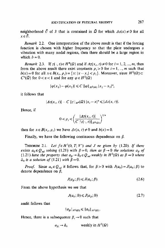
Remark 2.2. One interpretation of the above result is that if the forcing function is chosen with higher frequency so that the plate undergoes a vibration with many nodal regions, then there should be a large region in which b = 0.
Remark 2.3. If z( ., t)eH4(L?) and if dz(xi, t) #O for i= 1,2, . . . . m, then from the above result there exist constants pi > 0 for i = 1, . . . . m such that b(x) = 0 for all x E B(x,, pi) = {x: Ix - xi1 -K pi}. Moreover, since H*(a) c C’(n) for 0 <u < 1 and for any q E H*(G)
Icp(xl)-cp(x*)l GC lldlH2(f2) lx1 -xJa,
it follows that
IdZ(Xi, t)l -C llZllH4(Q) Ixi-xIaG IdzCx7 ‘11’
Hence, if
( ldztxi7 t)l >
l/a o<p,<
c II4 .? tlll”qn)
then for x E B(xi, pi) we have dz(x, t) # 0 and b(x) = 0.
Finally, we have the following continuous dependence on B.
THEOREM 2.1. Let f~ H’(0, T; V’) and J ne given by ( 1.20). If there exists a, E Qad solving (1.21) with /3 = 0, then us j? + 0 the solutions ug of (1.21) huoe the property that ug + ii,, E Qad weakly in IfI’(IR) us B + 0 where CT0 is a solution of (1.21) with /?=O.
ProoJ: Since a, E Qad it follows that, for B > 0 with J(u,) = J(u,; /I) to denote dependence on /I,
J(q9; B) G 4%; a,.
From the above hypothesis we see that
quo; 0) < J(us; 0)
andit follows that
lb&l ffqq G Iboll “2(ra).
(2.6)
(2.7)
Hence, there is a subsequence /Ii + 0 such that
q3, + 4 weakly in H’(a)
288 L. W. WHITE
and weakly in L’(0, T; V)
weakly in L2(0, T; H).
Now ii, E Qad since Qnd is closed in the weak topology of H’(Q). Thus, it follows that
J(q); 0) 2 J(q); 0).
But from the limit as /I + 0 in (2.6), we see that
and we have the result.
COROLLARY 2.1. For .Z satisfying (1.20)(i). Zf there exists a unique a, E Qad such that ~(a,,) = z, then a4 + a0 weakly in Z-Z2(0).
3. REGULARITY OF THE OPTIMAL ESTIMATORS
In this section we assume that the bilinear form a( ., .) is given as in (1.4) or (1.5). We determine regularity properties of optimal estimators the exist- ence of which was demonstrated in Section 1. Our approach is to apply a generalized version of the Kuhn-Tucker Theorem and to analyze the regularity of the solutions of the Euler equations of Lagrangian.
We begin by determining conditions under which the variation of the solution of (1.19) with respect to the parameter a exists. For concreteness we assume the bilinear form a( ., .) is given by (1.4), the case for (1.5) being similar. To this end let h E L”(G) and let E > 0 be sufhciently small that
u+eh>;>O a.e. in 52
and set
u, = (~(a + .zh) - u(u))/&.
It is clear that u, satisfies the equations
(o,,,(t), cp > + s, (a + &h)(x) due(x, t) h(x) dx
= - s h(x) du(x, t; a) dq$x) dx R (3.1)
IDENTIFICATIONOFFLEXURALRIGIDITY 289
with initial conditions
u,(O) = u,(O) = 0. (3.2)
Now the right side of (3.1) defines a continuous linear mapping H: V --) V by
I hAqA+ dx = (Hq, II/). R
Accordingly, Eq. (3.1) becomes
<u,,,,~)+f~(u+~h)(X)A A u x, t) AS(x) dx= -(Hu(., t), cp). (3.3)
From Corollary 1.1 iffc H’(0, T; H), then U, E K Hence, it follows that Hu belongs to H’(0, T; V’). As a consequence of Proposition 1.3 we may pass to the limit in (3.3) as E -to to obtain for u=&(a)(h)
= - 5 h(x) Au(x, t; a) Aq(x) dx a.e. t E (0, T) (3.4) R
u(0) = u,(O) = 0.
We have demonstrated the following
PROFQSITION 3.1. Let f E H’(0, T; H). Then giuen h E L”(Q) the uariu- tion of u(u) with respect to h exists and satisfies (3.4).
With this preparation we may now calculate the variation of the tit-to- data function J. Hence, we see that if the hypothesis of Proposition 3.1 is satisfied then the following holds.
COROLLARY 3.1. Let f e H’(0, T; H).
Then the uuriution of J(u) in the direction of h E H’(G) is given by
(i) GJ(u)h=2fTj (u(u)-z)udxdt+2/J(u,h),z 0 R
or (3.5)
(ii) SJ(u)h = 2 joTigl (4x,, t; u) -zi(t)Ndx,, u(t)> + Mu, h)s,
where u is the solution of (3.4).
290 L. W. WHITE
Let us assume
6) z E L2(0, T; H)
Introducing the adjoint system
(3.6)
6) (p,,(t), cp > + a(p(t), cp) = (u(c a) - 4th cp) in (0, T)
P(T)=Pt(T)=O (3.7)
where cp E V, we observe that by Remark 1.3 the initial value problem (3.7)(i) has a unique solution. Moreover, if we take
(ii) zi E H’(0, T) for i = 1, . . . . w (3.6)
and introduce the system
<P,,(t), cp > + 4t(t), cp = fj (U(Xi, ti a) - zi(f)) 6, in (0, T)
(ii) ,=l (3.7) P(T)=P,(T)=o,
We see from Theorem 1.1 and Corollary 1.1 that there exists a unique solution.
COROLLARY 3.2. Let f E H’(0, T; H) and u,, = u, = 0. Then the variation of 6J(a) in the direction of h E H’(a) is given by
W4h=2ja(j-oT Ap(x, t) Au(x, t; a) dt >
h(x) dx + 2fi(a, h)“z (3.8)
for both (1.20)(i) and (ii) where p satisfies (3.7)(i) and (ii), respectively, and in the case of (3.7)(ii) the observations zi are taken to belong to H’(0, T) for i = 1, 2, . . . . 0.
Proof: Equation (3.8) follows by applying the Green theorem [14, 151 to (3.4) and (3.7)(i) and (ii) to rewrite (3.5)(i) and (ii). Finally, an applica- tion of Fubini’s theorem [8] yields (3.8).
Remark 3.1. From the assumption that f 6 H’(0, T; H) we see from Corollary 1.1
AUE H’(0, T; H).
Further, for p a solution of either adjoint Eq. (3.7)(i) we see that
APE L’(O, T; H).
IDENTIFICATION OF FLEXURAL RIGIDITY 291
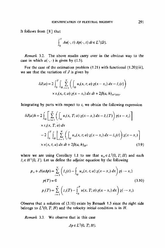
It follows from [8] that
s =du(., t)dp(*, t)dtEL’(B). 0
Remark 3.2. The above results carry over in the obvious way to the case in which a( ., .) is given by (1.5).
For the case of the estimation problem (1.21) with functional (1,2O)(iii), we see that the variation of J is given by
u,(x, t; a) x(x-xi) dx - ii(t) >
x u~(x, C a) x(x-xi) dx dt + 2/Va, h)Hzca).
Integrating by parts with respect to t, we obtain the following expression
aJ(,P=2~a[ i (jQ u,(x, T;a)~(x-xi)dx-ii(T) i=l
x u,(x, T; iz) dx
u,,(x, t; a) x(x-xi) dx - ii,(t) > 1 x(x-xi)
x u(x, t; a) dx dt + 2/?(a, h)“z (3.9)
where we are using Corollary 1.1 to see that u,, E L2(0, T; H) and each ii E H’(0, T). Let us define the adjoint equation by the following
Ptt+4ah)= f i= 1
P(T) = 0
u,,(x, t; a) x(x - xi) dx x( I - xi)
(3.10)
u(x, T,a)~(x-xi)dx x(.-xi).
Observe that a solution of (3.10) exists by Remark 1.3 since the right side belongs to L2(0, T; H) and the velocity initial condition is in H.
Remark 3.3. We observe that in this case
Lip E L2(0, T; H).
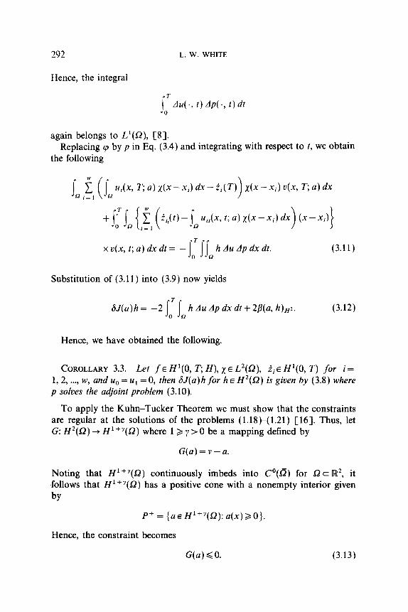
292 L. W. WHITE
Hence, the integral
.F 7’
Au(., t)Ap(., t)dt 0
again belongs to L’(Q), [S]. Replacing cp by p in Eq. (3.4) and integrating with respect to t, we obtain
the following
u&x, T, a) x(x -xi) dx - i,(T) x(x -xi) u(x, T, a) dx
ut,(x, t; a) x(x - xi) dx
x v(x, t; a) dx dt = - IoT [JQ h AU Ap dx dt. (3.11)
Substitution of (3.11) into (3.9) now yields
GJ(a)h = -2 ib7 IQ h Au Ap dx dt + 2/I@, h),+ (3.12)
Hence, we have obtained the following.
COROLLARY 3.3. Let f~H’(0, T; H), XE L*(Q), i,~f?‘(O, T) for i= 1, 2, . ..) w, and u0 = uI = 0, then GJ(a)hfor h E H*(Q) is given by (3.8) where p solves the aa!joint problem (3.10).
To apply the Kuhn-Tucker Theorem we must show that the constraints are regular at the solutions of the problems (1.18k(1.21) [16]. Thus, let G: H*(Q) + H’+“(Q) where 12 y >O be a mapping defined by
G(u)=v-a.
Noting that Iv?‘+~(SZ) continuously imbeds into Co(B) for Q c lR*, it follows that H’+“(Q) has a positive cone with a nonempty interior given by
P+ = (uEH’f~(S2): u(x)>O}.
Hence. the constraint becomes
G(u) < 0. (3.13)
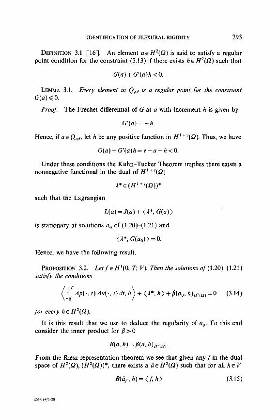
IDENTIFICATION OF FLEXURAL RIGIDITY 293
DEFINITION 3.1 [ 163. An element a E H2(s2) is said to satisfy a regular point condition for the constraint (3.13) if there exists h E ZY2(sZ) such that
G(a) + G’(a)h < 0.
LEMMA 3.1. Every element in Qad is a regular point for the constraint G(a) < 0.
Proof: The Frechet differential of G at a with increment h is given by
G’(a)= -h.
Hence, if a E Qad, let h be any positive function in H1 “(a). Thus, we have
G(a)+G’(a)h=v-a-h<O.
Under these conditions the Kuhn-Tucker Theorem implies there exists a nonnegative functional in the dual of H1 + y(sZ)
A* E (H1+y(sZ))*
such that the Lagrangian
L(a) = J(a) + (A*, G(a))
is stationary at solutions a, of (1.20)-(1.21) and
(A*, G(a,)) = 0.
Hence, we have the following result.
PROPOSITION 3.2. Let f E H’(0, T; V). Then the solutions of( 1.2Ok( 1.21) satisfy the conditions
t)M., t)dt, h >
+ (A*, h) +/Y(ao, hlHzCn,=O (3.14)
for every h E H2(SZ).
It is this result that we use to deduce the regularity of ao. To this end consider the inner product for /I > 0
From the Riesz representation theorem we see that given any f in the dual space of H2(12), (H’(Q))*, there exists a BE H2(12) such that for all he V
B(&, h) = CL h > (3.15)
469/144/l-20
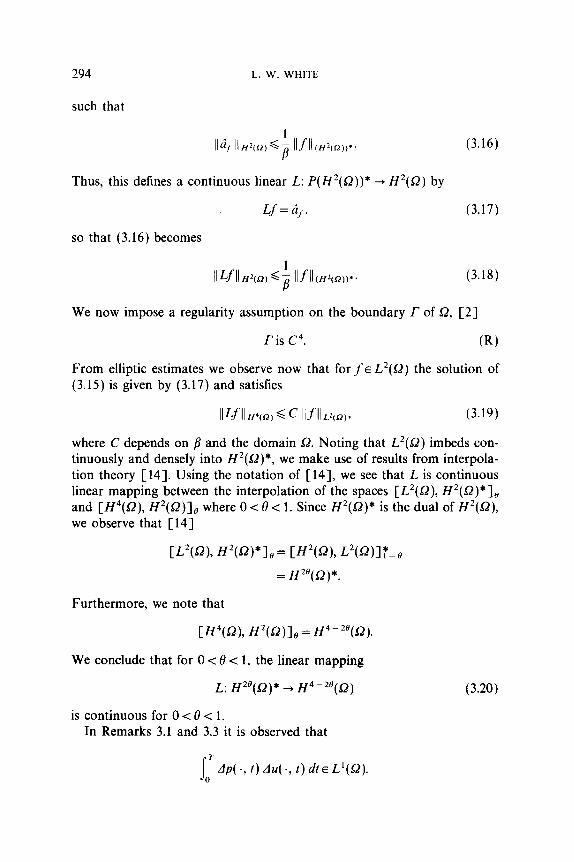
294
such that
L. W. WHITE
Thus, this defines a continuous linear L: P(H'(Q))* + H2(12) by
(3.16)
Lf=&. (3.17)
so that (3.16) becomes
IlLf II “2(O) G $ llfll (H+2))‘. (3.18)
We now impose a regularity assumption on the boundary r of Q, [2]
Tis C4. (RI
From elliptic estimates we observe now that for f~ L*(Q) the solution of (3.15) is given by (3.17) and satisfies
IlLf II w+(Q) d c llfll L2(L?)T (3.19)
where C depends on /I and the domain 52. Noting that L*(Q) imbeds con- tinuously and densely into H2(L2)*, we make use of results from interpola- tion theory [ 141. Using the notation of [ 141, we see that L is continuous linear mapping between the interpolation of the spaces [L*(Q), H*(Q)*& and [H4(Q), H2(S2)le where 0 < fI < 1. Since H*(O)* is the dual of H’(Q), we observe that [14]
CL2W, H*P)*l,= w*(Q), L2P)lL = H2e(SZ)*.
Furthermore, we note that
[H4(sz), H2(sz)ls = H4-2e(Q).
We conclude that for 0 < 8 < 1, the linear mapping
L:H*'(Q)* +H4-2e(Q)
is continuous for 0 < 0 < 1. In Remarks 3.1 and 3.3 it is observed that
I T
Llp(., t)du(., l)dlEL'(Q). 0
(3.20)
IDENTIFICATION OF FLEXURAL RIGIDITY 295
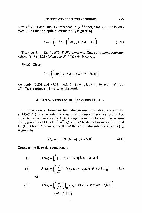
Now L’(Q) is continuously imbedded in (H’ +y(Q))* for y > 0. It follows from (3.14) that an optimal estimator a, is given by
a, = L ( J
-A*- ?lp(., t)du(., t)dt . 0 >
(3.21)
THEOREM 3.1. Let f E H(0, T, H), u. = u = 0. Then any optimal estimator soloing (1.18)-(1.21) belongs to H*+“(Q)for 0-es-c 1.
Proof: Since
i*+i’Ap(., t)du(., t)dtEH’+Y(Q)*, 0
we apply (3.20) and (3.21) with 8= (1 +y)/2,O<yl to see that a,~ H3-Y(f2). Setting s = 1 - y gives the result.
4. APPROXIMATION OF THE ESTIMATION PROBLEM
In this section we formulate finite dimensional extimation problems for (l.lS)-( 1.21) in a consistent manner and obtain convergence results. For concreteness we consider the Galerkin approximation for the bilinear form a( ., .) given by (1.4). Let VN, tP’, u:, and u;” be defined as in Section 1 and let (1.13) hold. Moreover, recall that the set of admissible parameters Qud is given by
Qad= {a~H~(Q):a(x)>v>O}. (4-l)
Consider the lit-to-data functionals
0) J”(a)=~‘IluN(I;a)-z(1)ll2Hdt+B lbll; 0
(ii)
(iii)
JN(CZ)=S:i$I (UN(Xjy t;a)-zi(t))2dt+B llall~ (4.2)
and
JN(a)=JoTi$l (s, > 2
X(Xj - x) ufqx, t; a) dx - i,(t)
xdt+D lbll:,.
296 L. W. WHITE
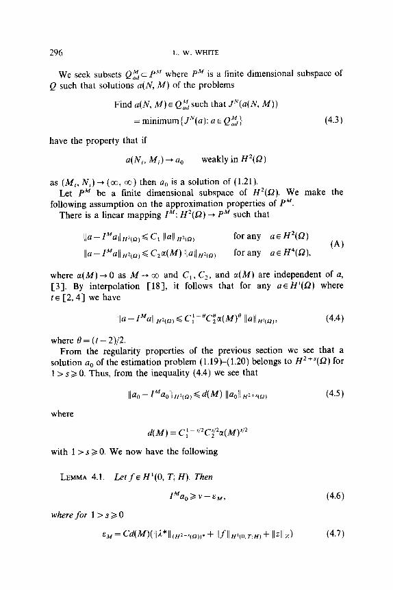
We seek subsets Q,“,c PM where P M is a finite dimensional subspace of Q such that solutions a(N, M) of the problems
Find a(N, M) E Qz such that JN(a(N, M))
= minimum {J”‘(a): a E Q,“,} (4.3)
have the property that if
a(Ni, Mi) + aO weakly in H*(8)
as (Mi, Ni) + (00, co) then a, is a solution of (1.21). Let PM be a finite dimensional subspace of H*(O). We make the
following assumption on the approximation properties of PM. There is a linear mapping Z”: H*(G) -+ PM such that
for any a E H*(G) (A)
for any a E H4(52),
where a(M) + 0 as A4 -+ co and C, , C2, and a(M) are independent of a, [3]. By interpolation [183, it follows that for any UE H’(a) where t E [2,4] we have
Ila--I”41f+2,< C:-°C;@4)o l~ull,t(,,, (4.4)
where 8 = (t - 2)/2. From the regularity properties of the previous section we see that a
solution a, of the estimation problem (1.19)-( 1.20) belongs to ZZ2+S(9) for 1) s 2 0. Thus, from the inequality (4.4) we see that
Ila, - IMa Hi < dt”) IbOll H2+S(R) (4.5)
where
d(M) = c: -s’2csl’a(M)“‘” with 1 > s > 0. We now have the following
LEMMA 4.1. Let f~ H’(0, T; H). Then
Z”aoav--EM, (4.6)
where for 1 >s>,O
E M = C~(~)(11~*11(H2-“(n))* + Ilf IIH’(O,T;H) + llzllZ) (4.7)
IDENTIFICATION OF FLEXURAL RIGIDITY 297
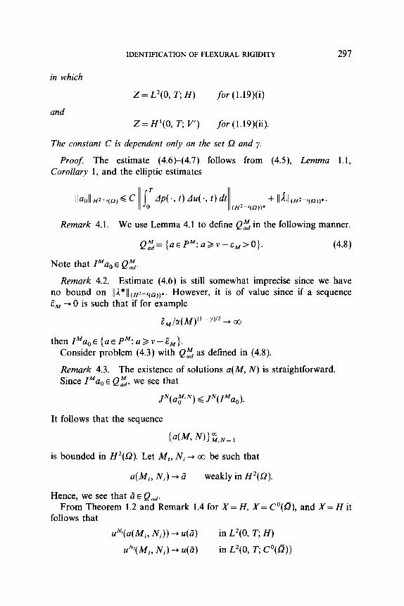
in which
z = L2(0, T; H) for (1.19)(i)
and Z=H’(O, r; V) for (l.l9)(ii).
The constant C is dependent only on the set Sz and y.
Proof: The estimate (4.6)-(4.7) follows from (4.5), Lemma 1.1, Corollary 1, and the elliptic estimates
Remark 4.1. We use Lemma 4.1 to define Qz in the following manner.
Q~={a~P”:a>v-&M>O}. (4.8)
Note that IMao E Qz.
Remark 4.2. Estimate (4.6) is still somewhat imprecise since we have no bound on IlA*Il(H2-s(njj.. However, it is of value since if a sequence E, -+ 0 is such that if for example
E”&+i4p - yv2 + co
then I”aoE(aEPM:a>v-EM}. Consider problem (4.3) with Q,“, as defined in (4.8).
Remark 4.3. The existence of solutions a(M, N) is straightforward. Since IMao E Qz, we see that
JN(ayN ) 6 JN(IMao).
It follows that the sequence
Ia(W NIZ,N=l
is bounded in H*(Q). Let Mi, Ni + cc be such that
a(M,, Nj) + d weakly in H*(a).
Hence, we see that d E Q,,. From Theorem 1.2 and Remark 1.4 for X= H, X= C’(8), and X= H it
follows that
uN’(a(Mi, Ni)) -+ u(Z) in L*(O, T; H)
UN’(Mi, Ni) --, u(Z) in L*(O, T; C’(0))
298 L. W. WHITE
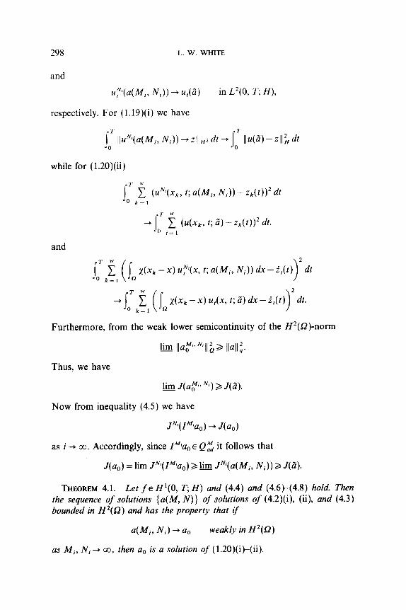
and
u;Y’(“(Mjt Ni)) + ut(n)
respectively. For (1.19)(i) we have
in L*(O, T; H),
jar llUN’(a(Mi,Ni))jzllHZdt~ joT Il”(ii)-zllffdt
while for (1.2O)(ii)
(uNJ(xk, t; u(M,, Ni)) - zk(t))* dr
(t&r, t; ii) - zk(t))’ dt.
and
x(x, -x) uF(x, t; a(hf,, Ni)) dx - i,(t)
x(x, -x) u,(x, t; ii) dx - i,(t)
Furthermore, from the weak lower semicontinuity of the H*(n)-norm
lim Ila,M’, NzII; 2 Ilull ;.
Thus, we have
lim J(up “‘) 2 J(C).
Now from inequality (4.5) we have
JN’(ZMkzo) -+ J(u,)
as i -+ co. Accordingly, since Z”?zo E Q,“, it follows that
J(u,) = lim JN~(ZMkzo) 3 l& JNju(Mi, Ni)) 3 J(G).
THEOREM 4.1. Let JE H’(0, r; H) and (4.4) and (4.6)-(4.8) hold. Then the sequence of solutions {u(M, N)} of solutions of (4.2)(i), (ii), and (4.3) bounded in H*(G) and has the property that if
d”i, Ni) + uO weakly in H*(Q)
us Mi, Ni + co, then a, is a solution of (1.2O)(ik(ii).
IDENTIFICATION OF FLEXIJRAL RIGIDITY 299
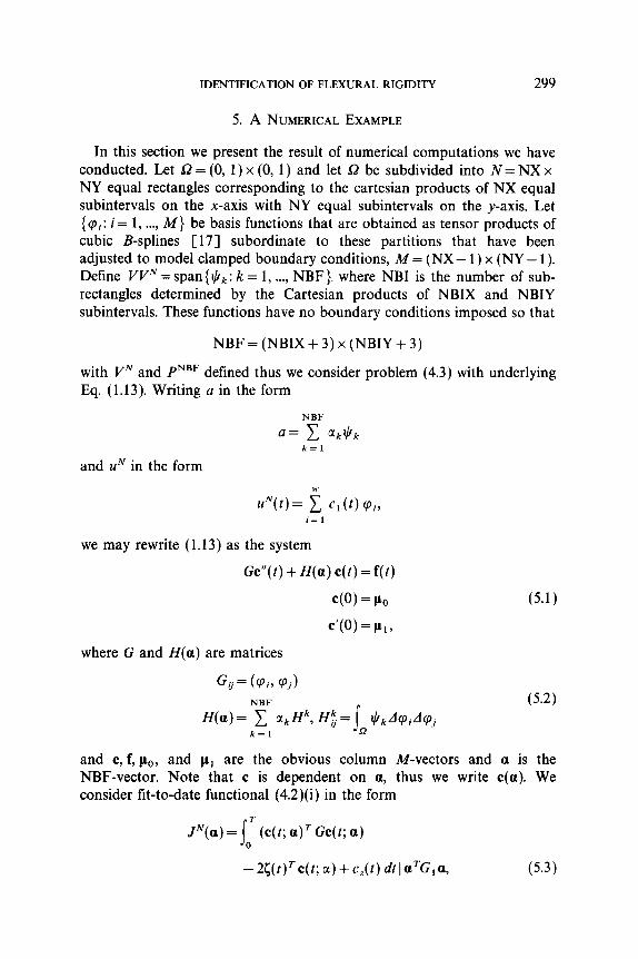
5. A NUMERICAL EXAMPLE
In this section we present the result of numerical computations we have conducted. Let Q = (0, 1) x (0, 1) and let 51 be subdivided into N = NX x NY equal rectangles corresponding to the Cartesian products of NX equal subintervals on the x-axis with NY equal subintervals on the y-axis. Let {q,: i= 1, . . . . M} be basis functions that are obtained as tensor products of cubic B-splines [17] subordinate to these partitions that have been adjusted to model clamped boundary conditions, M= (NX- 1) x (NY - 1). Define VVN=span{$,: k= 1, . . . . NBF}. where NBI is the number of sub- rectangles determined by the Cartesian products of NBIX and NBIY subintervals. These functions have no boundary conditions imposed so that
NBF = (NBIX + 3) x (NBIY + 3)
with VN and PNBF defined thus we consider problem (4.3) with underlying Eq. (1.13). Writing a in the form
NBF
a= C aklClk k=l
and zP’ in the form
u”(t)= i cl(t) cp,, i= I
we may rewrite (1.13) as the system
Gc”(t)+H(a)c(t)=f(t)
c(O) = PO
c’(O) = Pl,
(5.1)
where G and H(a) are matrices
NBF
s
(5.2) H(a)= c akHk, Hi= Il/kAViAVj
k=l a
and c, f, po, and pi are the obvious column M-vectors and a is the NBF-vector. Note that c is dependent on a, thus we write c(u). We consider lit-to-date functional (4.2)(i) in the form
f”(u) = j’ (c(t; u)~ Gc(t; a) 0
(5.3)
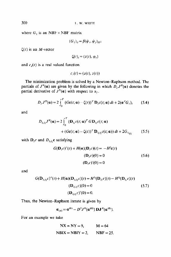
300 L. W. WHITE
where G, is an NBF x NBF matrix
c(t) is an M-vector
(GI Iv= B($i, $j)H*
L(t); = (z(t), cp,)
and c,(t) is a real valued function
c,(t) = (z(t)9 z(t))
The minimization problem is solved by a Newton-Raphson method. The partials of J”(a) are given by the following in which D,.JN(a) denotes the partial derivative of J”(a) with respect to uI.
D,J”(a)=2~T(Gc(f;a)-~(r))TD,c(f;u)dc+2(uTGl), (5.4) 0
and
D/J”‘(u) = 2 I’(D/,c(t, u)~GD,&; a) 0
+ (WC a) - Uf))T D,,,,c(K a)) dt + 2G1,,,2 (5.5)
with D,c and DI,,zc satisfying
G(D,c)“(t) + H(u)(D,c)(t) = -H/c(t)
P,c)(O) = 0
(D,c)‘(O) = 0
and
G(D,,,zc)“(t) + ff@W,,,,W) = H”(D,,W - ff’*(D,,W
(D,,,,cW) = 0
(D,,,,cW) = 0.
Thus, the Newton-Raphson iterate is given by
a(,, = do) - D2JN(cdo)) DJN(do’).
For an example we take
NX=NY=9, M = 64
NBIX = NBIY = 2, NBF = 25.
(5.6)
(5.7)
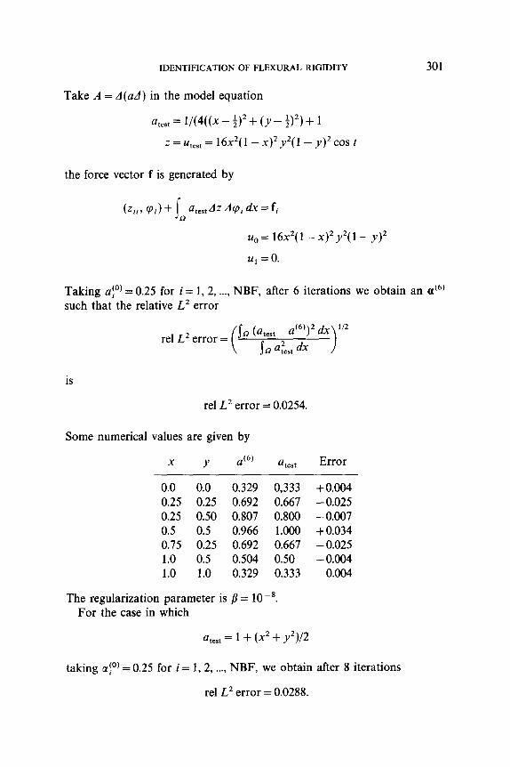
IDENTIFICATION OF FLEXURAL RIGIDITY 301
Take A = A(&) in the model equation
a test = 1/(4((x- $,‘+ (y- ;)2)+ 1
z = kst = 16x2( 1 - x)~ y’( 1 - y)’ cos t
the force vector f is generated by
(Ztl, ‘Pi)+ jQatestdzdVidx=fi
uo= 16x2(1 -~)~y~(l -Y)~
Ml = 0.
Taking ai . (‘) = 0 25 for i = 1, 2, . . . . NBF, after 6 iterations we obtain an uC6) such that the relative L2 error
rel L2 error = SD (atest- u@))~ dx I"
s a a:,,, dx >
is
rel L2 error = 0.0254.
Some numerical values are given by
X Y &5) %t Error
0.0 0.0 0.329 0,333 +0.004 0.25 0.25 0.692 0.667 -0.025 0.25 0.50 0.807 0.800 -0.007 0.5 0.5 0.966 1.000 +0.034 0.75 0.25 0.692 0.667 -0.025 1.0 0.5 0.504 0.50 -0.004 1.0 1.0 0.329 0.333 0.004
The regularization parameter is /I = 10-s For the case in which
atest = 1 + (x’ + y2)/2
taking ai’) = 0.25 for i = 1, 2, . . . . NBF, we obtain after 8 iterations
rel L2 error = 0.0288.
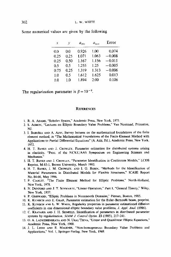
302 L. W. WHITE
Some numerical values are given by the following
X I? Q(8) a test Error
0.0 0.0 0.926 1.00 0.074 0.25 0.25 1.071 1.063 - 0.008 0.25 0.50 1.167 1.156 -0.011 0.5 0.5 1.255 1.25 - 0.005 0.75 0.25 1.319 1.313 -0.006 1.0 0.5 1.612 1.625 0.013 1.0 1.0 1.894 2.00 0.106
The regularization parameter is /I = lo-*.
REFERENCES
1. R. A. ADAMS, “Sobolev Spaces,” Academic Press, New York, 1975. 2. S. AGMON, “Lectures on Elliptic Boundary Value Problems,” Van Nostrand, Princeton,
NJ. 3. I. BABUSKA AND A. Azrz, Survey lectures on the mathematical foundations of the linite
element method, in “The Mathematical Foundations of the Finite Element Method with Applications to Partial Differential Equations” (A. Aziz, Ed.), Academic Press, New York, 1972.
4. H. T. BANKS AND J. CROWLEY, Parameter estimation for distributed systems arising in elasticity, “Proc. of the NCKU/AAS Symposium on Engineering Sciences and Mechanics.”
5. H. T. BANKS AND J. CROWLEY, “Parameter Identification in Continuum Models,” LCDS Reprint, M-83-1, Brown University, March 1983.
6. H. T. BANKS, J. M. CROWLEY, AND I. G. ROSEN, “Methods for the Identification of Material Parameters in Distributed Models for Flexible Structures,” ICASE Report No. 84-66, May 1986.
7. P. CIARLET, “The Finite Element Method for Elliptic Problems,” North-Holland, New York, 1978.
8. N. DUNFORD AND J. T. SCWWARTZ, “Linear Operators,” Part 1, “General Theory,” Wiley, New York, 1957.
9. P. GRISWARD, “Elliptic Problems in Nonsmooth Domains,” Pitman, Boston, 1985. 10. K. KUNISCH AND E. GRAIF, Parameter estimation for the Euler-Bernoulli beam, preprint. 11. K. KUNISCH AND L. W. WHITE, Regularity properties in parameter estimationof diffusion
coetlicients in one dimensional elliptic boundary value problems, J. Appl. Anal. (1986). 12. C. KRAVARIS AND J. H. SEINFELD, Identification of parameters in distributed parameter
systems by regularization, SIAM J. Control Oprim. 23 (1985), 217-241. 13. 0. A. LADYZSHENSKAYA AND N. URAL’TSEVA, “Linear and Quasilinear Elliptic Equations,”
Academic Press, New York, 1968. 14. J. L. LIONS AND E. MAGENES, “Non-homogeneous Boundary Value Problems and
Applications,” Vol. 1, Springer-Verlag, New York, 1969.
IDENTIFICATION OF FLEXURAL RIGIDITY 303
15. J. L. LIONS, “Control of Systems Governed by Partial Differential Equations,” Springer- Verlag, Berlin/New York, 1971.
16. D. G. LUENBERGER, “Optimization by Vector Space Methods,” Wiley, New York, 1971. 17. M. SCHULTZ, “Spline Analysis,” Prentice-Hall, Englewood Cliffs, NJ, 1973. 18. L. SCHLJMAKER, “Spline Functions Basic Theory,” Wiley, New York, 1981. 19. R. TEMAM, “Navier-Stokes Equations and Numerical Analysis,” North-Holland,
New York, 1979. 20. S. TIMOSHENKO AND S. WOINOWSKY-KRIEGER, “Theory of Plates and Shells,”
McGraw-Hill, New York, 1959. 21. L. W. WHITE, Estimation of elastic parameters in beams and certain plates: H’ regulariza-
tion, J. Optim. Theory Appl., in press.
Printed in Belgium