Embed Size (px)
Citation preview
1
IDENTIFICATION OF CONSTRUCTION PROJECT PROBLEMS AND
THEIR IMPACTS ON PROJECT SUCCESS
By
SEONG JIN KIM
A DISSERTATION PRESENTED TO THE GRADUATE SCHOOL
OF THE UNIVERSITY OF FLORIDA IN PARTIAL FULFILLMENT
OF THE REQUIREMENTS FOR THE DEGREE OF
DOCTOR OF PHILOSOPHY
UNIVERSITY OF FLORIDA
2009

2
© 2009 Seong Jin Kim

3
To my family;
Keun Ho Kim, Kye Haeng Jo, Won Sook Kim, and Won Jae Kim
4
ACKNOWLEDGMENTS
I really thank all my families in Korea for believing in me and supporting me, no matter
where I am and what I do. Besides my families, there are many friends who are helping me
unconditionally whenever I need help. Without their help, I would not have been able to be who
I am right now. Those friends are Seong Hoon (Seth) Lee, Hyang Sil (Bonnie) Park, Sook Hee
(Harriet) Choi, Janghowan Choi, Dae Keun Shin, Byung Cheol Kim, Zee Woon Lee, Tae Kook
Lee, Ji Yong Kim, and Whan Soon Yang. In addition to these friends, Stan Hudson, Justin
Burns, Ferdinand DeJesus, and Erika Sanchez are also a part of help and support group. Finally
my old time English teacher Yoon Sik Goh and my former advisor, Stuart Anderson, at Texas
A&M University have to also be thanked
The special thanks should go to Dr. Raymond Issa. He is the one who has enabled me to
reach whre I am right now. Without his help, guidance, and advice, I would not have been able
to pursue my dream. I would also like to thank my committee members who are Dr. Ian Flood,
Dr. R. Edward Minchin, Jr., Dr. E. Douglas Lucas, and Dr. Randy Chow as well. They always
guided me into the right direction of my research. Their guidance helped me improve myself
and realize my potential as a scholar. I am really lucky to have them all on my committee and
spend some time with them.
All my experience in the Rinker School at the University of Florida is priceless and I love
and am proud to be a part of this program. I also thank Dr. Richard Smailes for giving me a
chance to be a teaching assistant of BCN 5789 and BCN 4787 (Capstone). The experience I
have had as a TA has been very helpful for in getting me ready to teach classes. It gives me an
eye opener of teaching world. I really thank all the students who take the capstone class from
Spring 07 to Spring 08 while I am a TA of that class. All the comments and opinions they
provide me are helpful as well. I wish I could write down their names all here but unfortunately

5
I cannot because it will be more than two hundred students. I am sure that they will understand
the situation here. But I do remember them all even though their names are not shown here.
During this research, I have lots help from my BCN classmates from classes of 07 and 08,
especially Nicole Singleton, Alex Curry, Jessica Ligator, and Kristi Johnson. They and their
colleagues at work unconditionally participated in this research. Some of my colleagues from
Balfour Beatty also helped me out. They are Miles Gibbs, Kurtis Wright, Mike Neumann, Nick
Wegener, Joe Smith, and John Ricker. I really thank them all. Saying “Thank you” to them is
never enough.
I had never realized how lucky I was until I joined this program. I feel that I am really
lucky to have good people around me all the time. The past four years of my educational
experience the Rinker School showed me the direction of my near future work as an academic
scholar. I have been receiving something from people that I do care for and love. I think that
now is the time that I should give something back to them in return. I love to be here and am
glad that I did.
6
TABLE OF CONTENTS
page
ACKNOWLEDGMENTS ...............................................................................................................4
LIST OF TABLES .........................................................................................................................10
LIST OF FIGURES .......................................................................................................................14
LIST OF OBJECTS .......................................................................................................................16
ABSTRACT ...................................................................................................................................17
CHAPTER
1 INTRODUCTION ..................................................................................................................19
Problem Statement ..................................................................................................................21
Research Questions .................................................................................................................21
Purpose, Objectives, and Approach ........................................................................................22
Layout of Dissertation ............................................................................................................23
2 LITERATURE REVIEW .......................................................................................................24
Overview .................................................................................................................................24
Project Success Factors/Criteria .............................................................................................24
Factors Affecting the Success of a Construction Project ................................................24
Framework of Success Criteria for Design/Build Project ...............................................26
Project Performance Measure .................................................................................................27
Balanced Scorecard .........................................................................................................27
Project Definition Rating Index .......................................................................................29
Leading Indicators ...........................................................................................................32
Weight Computations in Index Models ..................................................................................34
Background ......................................................................................................................34
Concerns with Weights in Index Modeling .....................................................................38
Simple Multi-Attribute Rating Technique Using Swing (SMARTS).....................................41
3 STRATEGY AND DESIGN ..................................................................................................45
Overview .................................................................................................................................45
Development of Problems ......................................................................................................45
Data Collection .......................................................................................................................47
Data Transformation ...............................................................................................................48
Data Analysis ..........................................................................................................................49
Descriptive Statistics .......................................................................................................49
Data Tendency Analysis ..................................................................................................51
Methodology ...........................................................................................................................53
7
Background ......................................................................................................................53
Canonical Correlation ......................................................................................................55
Overview ..................................................................................................................55
Computation of canonical correlations ....................................................................56
Results of canonical correlations ..............................................................................56
Factor Analysis (Exploratory vs. Confirmatory) .............................................................59
Exploratory Factor Analysis (EFA) .................................................................................61
Overview ..................................................................................................................61
Number of factors with extraction methods .............................................................64
Confirmatory Factor Analysis (CFA) ..............................................................................67
Overview ..................................................................................................................67
CFA models for this research ...................................................................................70
Procedures for CFA Models ............................................................................................71
Overview ..................................................................................................................71
Crobach‟s (Coefficient) alpha ..................................................................................73
Average values of groups of each success parameter ..............................................75
Data normality ..........................................................................................................75
Computer package and goodness-of-fit test .............................................................77
Parameter estimate and significance test ..................................................................80
4 FACTOR ANALYSIS RESULTS .........................................................................................82
Overview .................................................................................................................................82
Cronbach‟s Alpha ...................................................................................................................83
Initial Cronbach‟s Alpha Values .....................................................................................83
Improvement of Coefficient Alpha Values .....................................................................84
Final Cronbach‟s Alpha Values .......................................................................................87
Average Value of Group .........................................................................................................88
Exploratory Factor Analysis (EFA) ........................................................................................89
Overview .........................................................................................................................89
Factor Extraction Technique ...........................................................................................90
Eigenvalue Greater Than 1.0 Method .............................................................................91
Scree Test Method ...........................................................................................................94
EFA Result Summary ......................................................................................................97
Normality Check .....................................................................................................................97
Confirmatory Factor Analysis (CFA) ...................................................................................100
Overview .......................................................................................................................100
Interpretation of Parameter Estimate Process ................................................................100
Initial Results for Each Success Parameter ...................................................................103
CFA Model Trimming ...................................................................................................105
Overview ................................................................................................................105
Critical ratio (CR) method ......................................................................................107
All possible combination of problem groups method ............................................110
Critical ratio (CR) vs. all possible combination .....................................................114
Final goodness-of-fit test indices ...........................................................................116
Parameter Estimate and Significance ............................................................................117
8
5 APPLICATION OF CFA MODEL OUTPUTS ...................................................................121
Background ...........................................................................................................................121
Single Multi-Attribute Rating Technique Using Swing Weight (SMARTS) .......................122
Overview .......................................................................................................................122
Computation of Input Values ........................................................................................122
Independency Properties of Values ...............................................................................124
Dominance of Problem Groups .....................................................................................129
Basic Concept of Application ...............................................................................................133
Overview .......................................................................................................................133
Scenario .........................................................................................................................134
Equation Example .........................................................................................................135
Denotation of input table ........................................................................................135
Weighted problem group ........................................................................................135
Degrees of problem severities ................................................................................136
Numeric Example ..........................................................................................................137
Using equal success priority weights .....................................................................137
Using unequal success priority weights .................................................................138
Using both unequal success priority weights and degrees of problem severity .....139
Summary ........................................................................................................................141
Development of Application .................................................................................................142
Overview .......................................................................................................................142
Application Software Program ......................................................................................143
Application Description .................................................................................................143
Validation of Application ..............................................................................................149
Overview ................................................................................................................149
Validation survey ...................................................................................................149
Validation survey output ........................................................................................150
6 CONCLUSIONS AND RECOMMENDATIONS ...............................................................157
Conclusions...........................................................................................................................157
Recommendations for Future Research ................................................................................159
APPENDIX
A 43 Potential Problems ...........................................................................................................162
B Definition of Each Problem Group .......................................................................................164
C Descriptive Statistics of 43 Problems ...................................................................................165
D Summary of Critical Ratio (CR) Method Procedure ............................................................171
E Summary of Raw Estimate and Its Unique Variances ..........................................................173
F Plots of Ten Pairs of Project Success Parameters .................................................................183

9
G Survey File ............................................................................................................................187
H Redrawn Regression Model ..................................................................................................191
LIST OF REFERENCES .............................................................................................................192
BIOGRAPHICAL SKETCH .......................................................................................................195
10
LIST OF TABLES
Table page
2-1 General procedure of an index model ................................................................................35
2-2 Example of project definition rating index ........................................................................36
2-3 Hackney‟s (1992) revised definition rating checklist ........................................................37
2-4 A six-point scale used for the questionnaire ......................................................................38
2-5 Generating five different weighted scores for cost parameter ...........................................38
2-6 Summary of three index models on weights ......................................................................39
3-1 Groups of potential problems.............................................................................................46
3-2 A six point scale .................................................................................................................48
3-3 Comparisons of current and rescaled .................................................................................49
3-4 Examples of problems with descriptive statistics ..............................................................50
3-5 Mean values of success parameters ...................................................................................51
3-6 Canonical correlations of cost parameter ...........................................................................57
3-7 Canonical correlations of schedule parameter ...................................................................57
3-8 Canonical correlations of quality parameter ......................................................................57
3-9 Canonical correlations of safety parameter........................................................................58
3-10 Canonical correlations of satisfaction parameter ...............................................................58
3-11 Heuristic EFA data .............................................................................................................62
3-12 Bivariate correlation matrix ...............................................................................................62
3-13 Eigenvalues for the example ..............................................................................................65
3-14 Equations and results of the model ....................................................................................69
3-15 Initial CFA model equations ..............................................................................................71
3-16 Equations for skewness and kurtosis .................................................................................76
3-17 Ranges of Skewness and Kurtosis .....................................................................................77
11
3-18 Goodness-of-fit test categories and its indices...................................................................79
4-1 Initial results for Cronbach‟s Alpha ...................................................................................84
4-2 Example of output of Cronbach‟s Alpha value in SPSS....................................................85
4-3 Incapability of improvement of Cronbahc‟s alpha value of SPSS ....................................86
4-4 Improvement of Cronbach‟s alpha value for CA in schedule............................................86
4-5 Improvement of Cronbach‟s alpha value for CA in quality ..............................................87
4-6 Improvement of Cronbach‟s alpha value for CO in safety ................................................87
4-7 Final Cronbach‟s alpha values ...........................................................................................88
4-8 EFA summary output of schedule......................................................................................92
4-9 EFA summary output of quality ........................................................................................93
4-10 EFA summary output of safety ..........................................................................................93
4-11 EFA summary output of satisfaction .................................................................................93
4-12 Summary of Eigenvalues of success parameters ...............................................................95
4-13 Output of normality check for cost ....................................................................................98
4-14 Output of normality check for schedule .............................................................................98
4-15 Output of normality check for satisfaction ........................................................................98
4-16 Output of normality check for quality ...............................................................................99
4-17 Output of normality check for safety .................................................................................99
4-18 Example of statistical significance of schedule using AL as base ...................................102
4-19 Example of statistical significance of schedule using CA as base ...................................102
4-20 Example of standard estimate ..........................................................................................103
4-21 Initial results of P values of CFA model ..........................................................................104
4-22 Summary of critical ratio (CR) procedure for schedule ...................................................108
4-23 Summary of best-fitted model using critical ratio (CR) method .....................................109
4-24 Summary of combinations of seven problem groups ......................................................111
12
4-25 Summary of six problem groups combinations for safety ...............................................113
4-26 Summary of best-fitted model using possible combination method ................................113
4-27 Comparisons of critical ratio and all possible combination .............................................114
4-28 Summary of goodness-of-fit indices ................................................................................116
4-29 Summary of standard estimate (factor loading) ...............................................................118
4-30 Equation forms for cost ....................................................................................................119
5-1 Conversion factor loadings for cost .................................................................................123
5-2 Summary of conversion values for all success parameters ..............................................124
5-3 Value difference between two parameters .......................................................................126
5-4 Value difference between two project success parameters ..............................................127
5-5 Correlations between project success parameters ............................................................127
5-6 Summary of variability ....................................................................................................128
5-7 Value difference between two problem groups ...............................................................130
5-8 Impacts of problems on each success parameter .............................................................135
5-9 Initial impacts with equal weights of 1 ............................................................................137
5-10 Weighted impacts of success parameters .........................................................................139
5-11 Weighted impacts of both unequal success parameters and degrees of problem
severity .............................................................................................................................140
5-12 The difference in ranking .................................................................................................142
5-13 Comparisons of original method and swing weights .......................................................145
5-14 Computation of proportional ratio of scores ....................................................................148
5-15 General summary of participants and project characteristics ..........................................151
5-16 Priority weights of six projects ........................................................................................151
5-17 Comparison of actual project and tool output ..................................................................153
A-1 43 Potential problems ......................................................................................................162
C-1 Descriptive statistics of 43 problems ...............................................................................165
13
D-1 Cost ..................................................................................................................................171
D-2 Quality..............................................................................................................................171
D-3 Safety ...............................................................................................................................171
D-4 Satisfaction .......................................................................................................................171
E-1 Cost ..................................................................................................................................173
E-2 Schedule ...........................................................................................................................175
E-3 Quality..............................................................................................................................177
E-4 Safety ...............................................................................................................................179
E-5 Satisfaction .......................................................................................................................181
14
LIST OF FIGURES
Figure page
1-1 Research approach .............................................................................................................22
2-1 Framework for factors affecting project success ...............................................................25
2-2 Criteria for project success.................................................................................................26
2-3 Framework for project success of design/build projects ....................................................27
2-4 Balanced scorecards ...........................................................................................................28
2-5 PDRI sections, categories, and elements ...........................................................................30
2-6 Example of final version of PDRI .....................................................................................32
2-7 Example output of LI tool ..................................................................................................34
3-1 A screen capture of evaluation worksheet .........................................................................47
3-2 Frequency histogram ..........................................................................................................52
3-3 Input matrix ........................................................................................................................56
3-4 A relationship between two variables ................................................................................60
3-5 Summary of latent factors and variables ............................................................................63
3-6 Scree plot. ..........................................................................................................................66
3-7 Example model. .................................................................................................................69
3-8 Initial CFA model for each success parameter ..................................................................70
3-9 CFA model procedure ........................................................................................................72
3-10 Distributions. ......................................................................................................................76
3-11 Screen capture of Amos .....................................................................................................78
4-1 The procedure of results.....................................................................................................82
4-2 Example of output of EFA for cost ....................................................................................91
4-3 Scree plot. ..........................................................................................................................96
4-4 Example of graphical input for CFA model ....................................................................101
15
4-5 Path diagram. ...................................................................................................................119
5-1 The plot of safety vs. satisfaction ....................................................................................128
5-2 Value difference between problem groups part 1 ............................................................131
5-3 Value difference between problem groups part 2 ............................................................132
5-4 Screen capture of Instruction worksheet for application .................................................144
5-5 Screen capture of input worksheet of application ............................................................146
5-6 Screen capture of output worksheet of application ..........................................................147
5-7 Regression model for validation of tool...........................................................................155
F-1 Cost vs. Schedule .............................................................................................................183
F-2 Cost vs. Quality ................................................................................................................183
F-3 Cost vs. Safety .................................................................................................................183
F-4 Cost vs. Satisfaction .........................................................................................................184
F-5 Schedule vs. Quality ........................................................................................................184
F-6 Schedule vs. Safety ..........................................................................................................184
F-7 Schedule vs. Satisfaction .................................................................................................185
F-8 Quality vs. Safety .............................................................................................................185
F-9 Quality vs. Satisfaction ....................................................................................................185
F-10 Safety vs. Satisfaction ......................................................................................................186
G-1 Worksheet of instruction ..................................................................................................187
G-2 Worksheet of survey part A through C ............................................................................188
G-3 Worksheet of survey part C through E ............................................................................189
G-4 Worksheet of survey part E..............................................................................................190
H-1 Redrawn regression model ...............................................................................................191

16
LIST OF OBJECTS
Object page
5-1 Potential problem identification tool as a Microsoft Excel file (.xls 41kb) .....................143
17
Abstract of Dissertation Presented to the Graduate School
of the University of Florida in Partial Fulfillment of the
Requirements for the Degree of Doctor of Philosophy
IDENTIFICATION OF CONSTRUCTION PROJECT PROBLEMS AND
THEIR IMPACTS ON PROJECT SUCCESS
By
Seong Jin Kim
December 2009
Chair: Raymond Issa
Cochair: Ian Flood
Major: Design, Construction and Planning
The traditionally accepted success parameters for construction projects are mainly cost and
schedule. There are new trends in how to define success and the number of success parameters
considered even though cost and schedule are still the most prevalent ones. The number and
priority of success parameters heavily depends on the owner. With respect to these trends,
determining the success of project is a hard and complicated procedure when a project faces
multiple problems simultaneously. The problems that practitioners or researchers face are: 1)
What are the relationships between these causes and their impacts on project success
parameters?; 2) Is it necessary to concern all problems for each different project success
parameter in terms of their negative impacts?; and 3) What problem is really considered when,
especially, the project has more than one success parameter with different priorities? The
proposed solutions are 1) to determine the relationships between problems and their impacts and
2) to select problems required to be considered for each project success parameter to meet multi-
project success parameters within different priorities. This will help ensure that the project
meets the required performance targets and adds value for all participants at the early phase of
18
project. Confirmatory factor analysis (CFA) models were used for testing the quality of
proposed solutions. The outputs of CFA were used for an application tool to select the most
critical problems under given circumstances such as parameter priorities and problems severity.
A single multi-attribute rating technique using swing (SMARTS) was the statistical tool used for
this study. The results of this research show the selection of critical problem groups under given
circumstances. In the future contractors, owners, and other project participants can use this
technique to more effectively conduct project reviews during the course of the project.
19
CHAPTER 1
INTRODUCTION
With respect to the development of technologies and new demands on markets, many
things in the construction industry have been changing rapidly and some new trends have
emerged. It appears impossible for the construction industry to break free from these current
trends. These trends would be the changes in the contract types, the development of
technologies and methodologies to manage the project problems effectively, and new demands
from owners (customers) on project outcomes. For example, even though, the highway industry
has used the lowest bid system for a long time, new innovative methods in contracting such as
„Method A+B‟ and „Lane Rental‟ have been proposed and/or are replacing the
lowest/competitive bid (Herbsman et al. 1995; Herbsman and Ellis 1992). A similar situation
could be easily found in commercial construction as well. There are many computer software
programs available that make construction management easier and more effective than ever
before. Owners‟ requests on projects have diversified as compared to the past. Owners may not
share the same concepts of project success parameters such as cost and schedule any longer. The
success of a project heavily depends on the owner‟s requirement. Apparently there are concerns
other than just cost and schedule in terms of project success parameters from an owner‟s
perspective. To keep their business rolling, it is critical for contractors to meet owners‟ demands
on projects in our rapidly changing industry.
One of the keys to meeting owners‟ demands is to manage the project problems a
contractor faces or will face in the near future because there exist probable relationships between
owners‟ demands and problems in affecting the success of a project success as defined by the
owner. Regarding the type of problems impeding success on construction projects, there are
prospectively two main questions. The first question is “What kinds of problems exist on
20
projects?” The second is “How do they differ from the problems of a few years ago?” The
answer to the first question could include material delays, the qualification of subcontractors and
architects, request for information (RFIs), and change order, etc. The answer to the second
question would be “No.” Unlike new trends and changes in demands, it does not appear that the
types of construction project problems have been changed that much. Nowadays, contractors
must manage multiple problems simultaneously.
The traditional project success parameters are cost and schedule. As mentioned above,
however, there are new, additional success parameters as defined and prioritized by the owner.
The new project success parameters could vary among projects and their owners. These new
parameters might be narrowed down to safety, quality, and owner‟s satisfaction. It is apparent
that any project in the immediate or near future has more than one or two success parameters.
There are numerous articles and abundant research available on project success parameters
and/or key performance indicators. This research addresses the fact that different problems have
different impacts on success parameters. But unfortunately it does not fully explain the
difference. There are two types of variables involved in this research and they are independent
and dependent variables. Although the project success index is represented as a dependent
variable, it is hard to define “success (success index)” because success is a combination of
different parameters (Griffith et al. 1999). Some dependent variables such as quality, safety, and
satisfaction are not available and/or easily accessible to researcher. These kinds of variables are
treated as confidential (safety incident rates and related indices) in a company and it is hard to
measure the degree of agreement (quality and safety). Therefore, the current studies and
research lack multi-project success parameters. Most studies have focused on cost and schedule
by predicting the outcomes during the course of project. Even though a predicted outcome may
21
give a guideline of how to manage the project at that moment, it does not specify where to
improve or fix the problems if the predicted outcome is not good. And also there are many
problems, factors, and indicators addressed without looking at their impacts on the project
success parameters.
This research is focused on finding the practices of general contractors and owners to
improve project performance during project execution. These practices could provide additional
insight into the success parameters while complimenting current approaches. This will help
ensure that the project meets the required performance targets and adds value for all participants
at an early stage of a project. The primary beneficiaries of this research include owners,
contractors, and other project participants.
Problem Statement
The problem statement is:
How much could project performance have been improved if the relationships between
problems and success parameters had been pre-identified in situations where there are multi-
project success parameters each with different priorities?
Research Questions
Five research questions have been developed for this research effort. These questions must
be investigated to address the research problem. The questions identified are as follows:
What are the common problems on projects?
What are the relationships between problems and their impacts on project success
parameters?
How different are these relationships when project success parameters have
different priorities?
How can critical problems be identified under given circumstances of multiple
success parameters and different priorities?
22
How can intangible variables (parameters) be measured in practice?
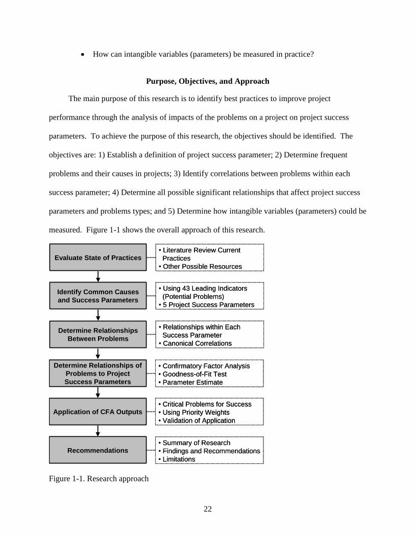
Purpose, Objectives, and Approach
The main purpose of this research is to identify best practices to improve project
performance through the analysis of impacts of the problems on a project on project success
parameters. To achieve the purpose of this research, the objectives should be identified. The
objectives are: 1) Establish a definition of project success parameter; 2) Determine frequent
problems and their causes in projects; 3) Identify correlations between problems within each
success parameter; 4) Determine all possible significant relationships that affect project success
parameters and problems types; and 5) Determine how intangible variables (parameters) could be
measured. Figure 1-1 shows the overall approach of this research.
Evaluate State of Practices• Literature Review Current
Practices
• Other Possible Resources
Identify Common Causes
and Success Parameters
• Using 43 Leading Indicators
(Potential Problems)
• 5 Project Success Parameters
Determine Relationships
Between Problems
• Relationships within Each
Success Parameter
• Canonical Correlations
Determine Relationships of
Problems to Project
Success Parameters
• Confirmatory Factor Analysis
• Goodness-of-Fit Test
• Parameter Estimate
Application of CFA Outputs• Critical Problems for Success
• Using Priority Weights
• Validation of Application
Recommendations• Summary of Research
• Findings and Recommendations
• Limitations
Figure 1-1. Research approach
23
Layout of Dissertation
Chapter 2 of this report provides an overview and additional background information on
this research. The review of current literature is presented. Chapter 3 describes the strategy and
design of this research. This includes an overview of the research approach and a development
of relationships between problems. A description of the data collection process and a discussion
of the data analysis are presented. Finally the research methodology will be discussed. Chapter
4 presents the general procedure of factor analysis for both exploratory and confirmatory
analysis and their results and findings of the study. Chapter 5 provides the development of an
application of outputs for reassessment of potential project problems. This includes an overview,
application, and validation of the methodology. Chapter 6 provides conclusions and then
recommendations for the usage of the methodology.
24
CHAPTER 2
LITERATURE REVIEW
Overview
To set up the framework of the research, a review was conducted of other research, current
trends, related topics, and methodologies. Although a literature review is the first step of this
research, it is very hard to find the same or at least similar topics or subjects among current
research. Some of the main concerns are performance/key indicators/factors in general
construction management and the process of how to develop performance indicators and how to
measure them by looking for success parameters. Project control, major issue areas, and how to
measure project performances will be discussed. This chapter mainly consists of three sections.
One is about the development of project success criteria and another is about the project
performance measure, and the last is about weights in index modeling. In addition to the main
sections, there will be a brief discussion on decision-making theory which may apply to the
development of an application for this research. More detailed information will follow.
Project Success Factors/Criteria
Factors Affecting the Success of a Construction Project
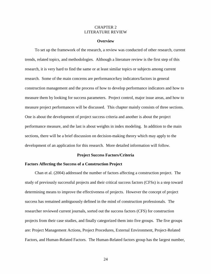
Chan et al. (2004) addressed the number of factors affecting a construction project. The
study of previously successful projects and their critical success factors (CFSs) is a step toward
determining means to improve the effectiveness of projects. However the concept of project
success has remained ambiguously defined in the mind of construction professionals. The
researcher reviewed current journals, sorted out the success factors (CFS) for construction
projects from their case studies, and finally categorized them into five groups. The five groups
are: Project Management Actions, Project Procedures, External Environment, Project-Related
Factors, and Human-Related Factors. The Human-Related factors group has the largest number,
25
22, of factors and the Project Procedures has the lowest number, two. The External Environment
has six factors, which are 1) Economic environment; 2) Social environment; 3) Political
environment; 4) Physical environment; 5) Industrial relations environment; and 6)
Technologically advanced. Figure 2-1 shows the five groups each with its set of factors.
Figure 2-1. Framework for factors affecting project success (Chan et al. 2004)
These factors could be the most influential if the factors affecting a project were
considered at the macro viewpoint. The chances to be an important factor for a project would be
lower than other factors. Chan et al. (2004) asserted that “project success is a function of
project-related factors, project procedures, project management actions, human-related factors
and external environment and they are interrelated and intrarelated.” They also pointed out the
potential relationships between factors and groups.
26
Framework of Success Criteria for Design/Build Project
Framework of success criteria for design/build projects (Chan et al. 2002) mainly
addressed the concept of a project success and what to measure to achieve project success in
design/build projects. The authors mention that measuring project success is a complex task
since success is intangible and can hardly be agreed upon. The general concept of project
success remains ambiguously defined because of varying perceptions. Each project participant
will have his or her own view of success. It depicts that owners, contractors, and architects have
a different perspective of project success. According to the authors, project success is the goal,
and the objectives of budget, schedule, and quality are the three normally accepted criteria to
achieve the goal. Each project has a set of goals to accomplish, and they serve as a standard to
measure performance. The authors addressed that the criteria for a construction project in
general can be classified under two main categories, one being hard, objectives, tangible, and
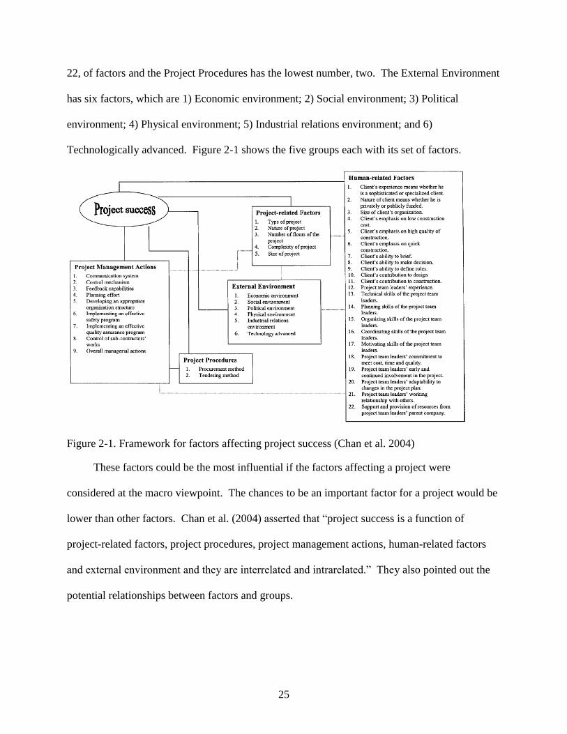
measurable, and the other soft, subjective, intangible, and less measurable. The integration of
success and criteria is shown in Figure 2-2.
As shown in Figure 2-2, some of examples are provided, for hard, objectives, tangible, and
measurable such as time, cost, quality, profitability, technical performance, completion,
functionality, health and safety, productivity, and environmental sustainability and for soft,
Figure 2-2. Criteria for project success (Chan et al. 2002)
27
subjective, intangible, and less measurable, such as satisfaction, absence of conflicts,
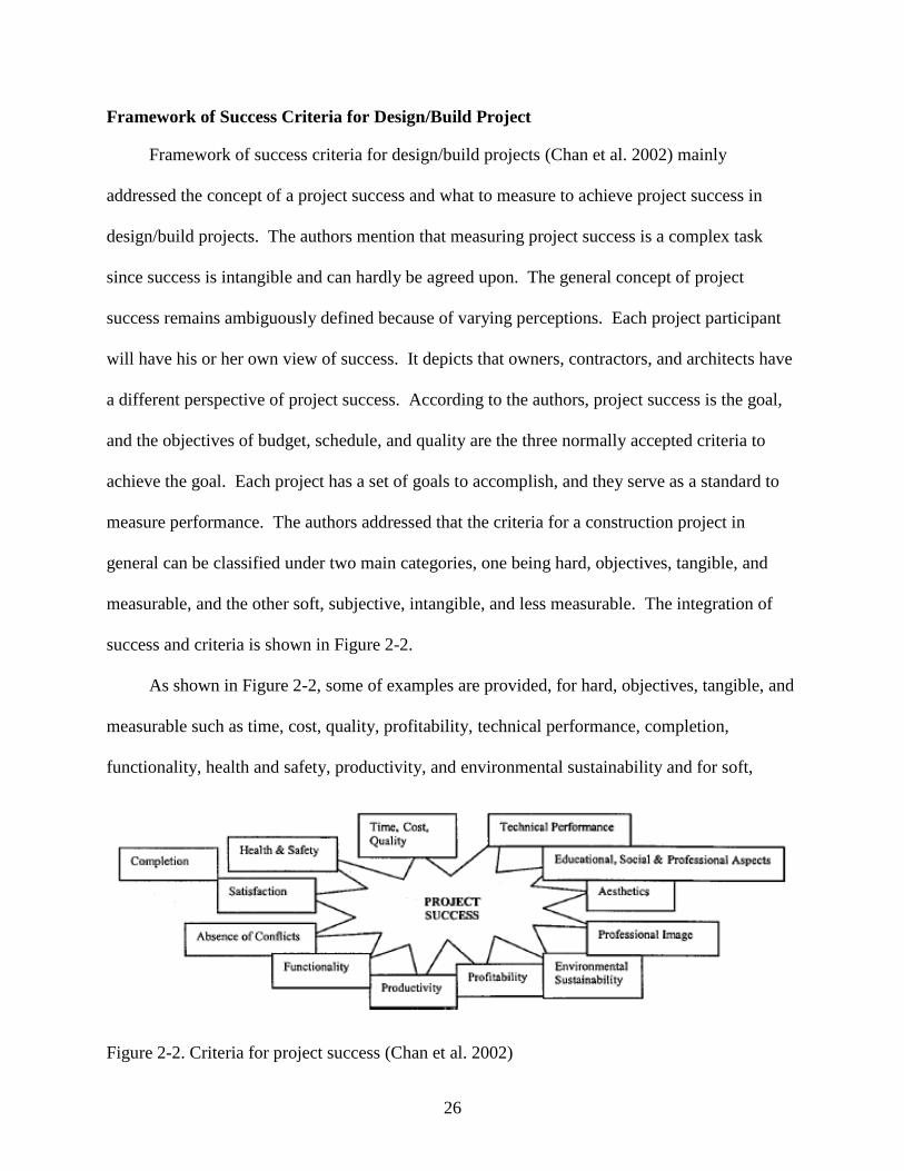
professional aspects. The unique idea proposed by this article is to add time concepts, like
phases of construction, to success criteria. With respect to the time parameter, measures of
success are different for each phase of the construction process (see Figure 2-3).
Phase Pre-Construction (Past) Construction (Current) Post-Construction (Future)
Objective Measure 1. Time 1. Time 1. Profitability
2. Cost 2. Cost
3. Health & Safety
Subjective Measure 1. Quality 1. Quality 1. Satisfaction of Key Project
2. Technical Performance 2. Technical Performance Participants, End-Users and
3. Satisfaction of Key Project 3. Productivity Outsiders
Participants 4. Satisfaction of Key Project - Completion
Participants - Functionality
- Conflict Management - Aesthetics
- Professional Image
- Educational, Social &
Professional Aspects
2. Environmental Sustainability
Time Horizon
Figure 2-3. Framework for project success of design/build projects (Chan et al. 2002)
As far as objective measures are concerned (see Figure 2-3), a maximum of three items are
in the construction phase (current) and only one item is in post-construction phase (future). For
the subjective measures, two major items with five sub-items are at the post-construction phase
(future) and three items are at pre-construction phase (past). The numbers of items in the
subjective measure are greater than the objective measure. It depicts that there are more
intangible criteria available in design/build projects in terms of successful projects.
Project Performance Measure
Balanced Scorecard
The balanced scorecard method (Kaplan and Norton 1992) tracks the key elements of a
company‟s strategy – from continuous improvement and partnerships to teamwork and global
28
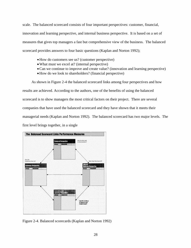
scale. The balanced scorecard consists of four important perspectives: customer, financial,
innovation and learning perspective, and internal business perspective. It is based on a set of
measures that gives top managers a fast but comprehensive view of the business. The balanced
scorecard provides answers to four basic questions (Kaplan and Norton 1992);
How do customers see us? (customer perspective)
What must we excel at? (internal perspective)
Can we continue to improve and create value? (innovation and learning perspective)
How do we look to shareholders? (financial perspective)
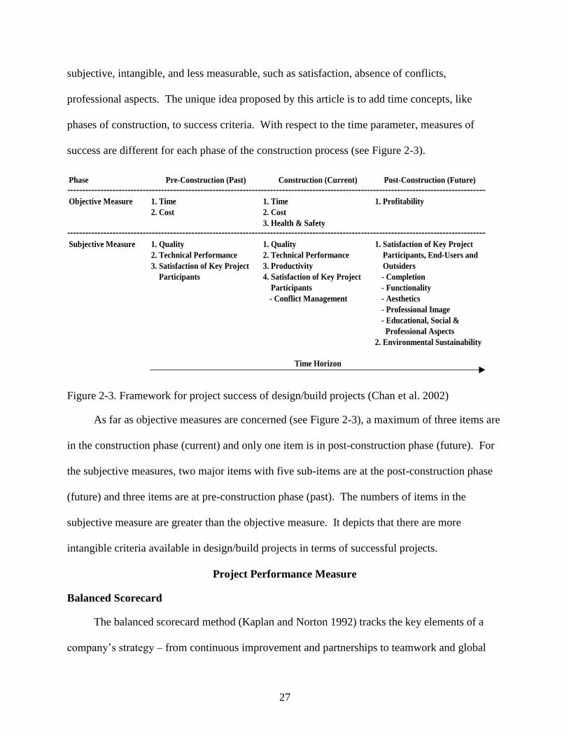
As shown in Figure 2-4 the balanced scorecard links among four perspectives and how
results are achieved. According to the authors, one of the benefits of using the balanced
scorecard is to show managers the most critical factors on their project. There are several
companies that have used the balanced scorecard and they have shown that it meets their
managerial needs (Kaplan and Norton 1992). The balanced scorecard has two major levels. The
first level brings together, in a single
Figure 2-4. Balanced scorecards (Kaplan and Norton 1992)
29
management report, many of the seemingly disparate elements of a company‟s competitive
agenda such as becoming customer oriented, shortening response time, improving quality, and
emphasizing teamwork at the manager level. The second level guards against sub-optimization
at senior management level, which means that it forces senior managers to consider all the
important operational measures together. It makes it possible for senior managers to make sure
that they use a balanced approach and to make sure improvement in one area has not been
achieved at the expense of another, hence, the name balanced scorecard.
The balanced scorecard is based on management strategies and their measures. It aids
managers in tracking their performances based on their strategies or goals and shows the
relationship between four different perspectives and the impacts on the results. These concepts
could be adopted to develop an application for this research. Project problems have different
impacts on project success parameters and each success parameters could have different priority
weights. The four perspectives of the balanced scorecard are equivalent to project success
parameters. The authors did not mention how to set up the strategies because strategies can be
different for different organizations or companies based on their needs or demand. But it shows
how companies or organizations have improved their performances and the degree of
improvement using the balanced scorecard.
Project Definition Rating Index
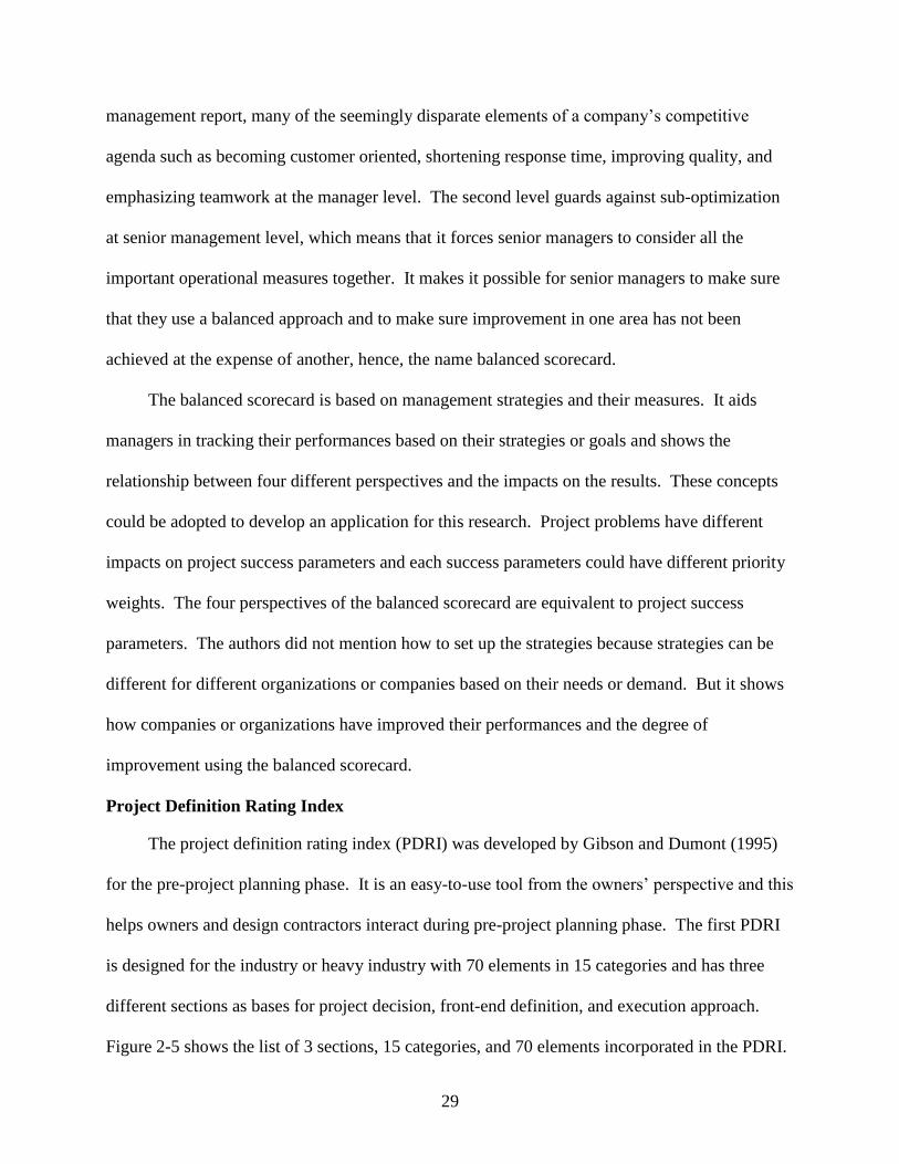
The project definition rating index (PDRI) was developed by Gibson and Dumont (1995)
for the pre-project planning phase. It is an easy-to-use tool from the owners‟ perspective and this
helps owners and design contractors interact during pre-project planning phase. The first PDRI
is designed for the industry or heavy industry with 70 elements in 15 categories and has three
different sections as bases for project decision, front-end definition, and execution approach.
Figure 2-5 shows the list of 3 sections, 15 categories, and 70 elements incorporated in the PDRI.
30
Figure 2-5. PDRI sections, categories, and elements (Gibson and Dumont 1995)
31
The PDRI is based on the scope definition, i.e. the degree of scope definition at the pre-project
planning phase. If the scope is well defined at that time, the impact on the project will be
positive later. The degree of scope definition consists of five levels (Level 1 through 5) and
definition of each level is as follows (Gibson and Dumont 1995):
1: Completion Definition
2: Minor Deficiencies
3: Some Deficiencies
4: Major Deficiencies
5: Incomplete or Poor Definitions
In the PDRI development stages, industry participants were asked to weigh elements by
level of scope definitions and there was no limit on weighing. The weighting value represents
each element‟s impact on total installed cost (TIC) stated as a percentage of the overall estimate.
Therefore the lower the value, the better project scope definition is. Finally all the data are
normalized by a 1,000 scale as the maximum score for the tool development. It represents the
sum of all values (70 elements) in level 5 of the scope definition and is equal to 1,000. The
scores of Levels 1 through 4 are rescaled proportionally compared to Level 5.
Figure 2-6 shows an example of the final version of PDRI. There is a difference in the
level of scope definitions compared to the initial version. An option of “Not Applicable” is
added into the level of scope definition. As mentioned earlier, the sum of Level 5 will be 1,000.
In the example, category L, Procurement Strategy is assigned a maximum score of 16 which is
the sum at Level 5 of items, L1, L2, and L3.
The maximum score of each item in Section L is 8, 5, and 3 for L1, L2, and L3
respectively. The score range of levels for an item L3 lies in between 0 for Level 1 and 5 for
Level 5. If any user defines the level of scope definition of 70 items, then fill the column of
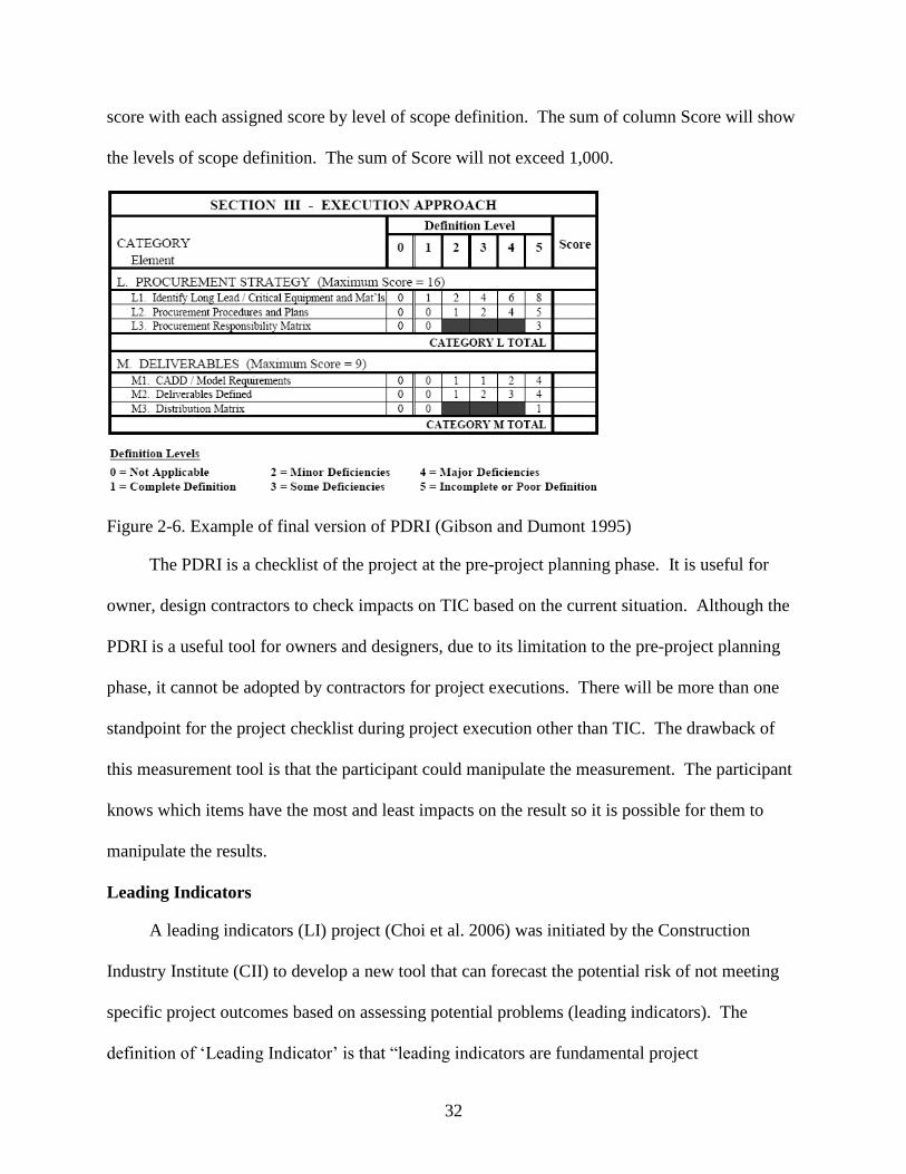
32
score with each assigned score by level of scope definition. The sum of column Score will show
the levels of scope definition. The sum of Score will not exceed 1,000.
Figure 2-6. Example of final version of PDRI (Gibson and Dumont 1995)
The PDRI is a checklist of the project at the pre-project planning phase. It is useful for
owner, design contractors to check impacts on TIC based on the current situation. Although the
PDRI is a useful tool for owners and designers, due to its limitation to the pre-project planning
phase, it cannot be adopted by contractors for project executions. There will be more than one
standpoint for the project checklist during project execution other than TIC. The drawback of
this measurement tool is that the participant could manipulate the measurement. The participant
knows which items have the most and least impacts on the result so it is possible for them to
manipulate the results.
Leading Indicators
A leading indicators (LI) project (Choi et al. 2006) was initiated by the Construction
Industry Institute (CII) to develop a new tool that can forecast the potential risk of not meeting
specific project outcomes based on assessing potential problems (leading indicators). The
definition of „Leading Indicator‟ is that “leading indicators are fundamental project
33
characteristics and/or events that reflect or predict project health. Revealed in a timely manner,
these indicators allow for proactive management to influence project outcomes” (Choi et al.
2006). Forty-three leading indicators were finally developed through three surveys and five
different project success parameters were identified. The five different success parameters were
cost, schedule, quality, safety, and owners‟ satisfaction. Each LI was evaluated in terms of each
successful outcome using a five-point scale. If an LI has the highest negative impact on any
success outcome, then five points will be assigned to it. If an LI has no negative impact on any
success outcome, then zero will be assigned. And the rest will be in between. Weights of
problems are based on aggregated scores. Based on this framework, a LI forecasting tool has
been developed. In the tool usage, each problem is assessed as follows (Choi et al. 2006):
1: Serious (100%)
2: Major (75%)
3: Moderate (50%)
4: Minor (25%)
5: None (0%)
Not Applicable
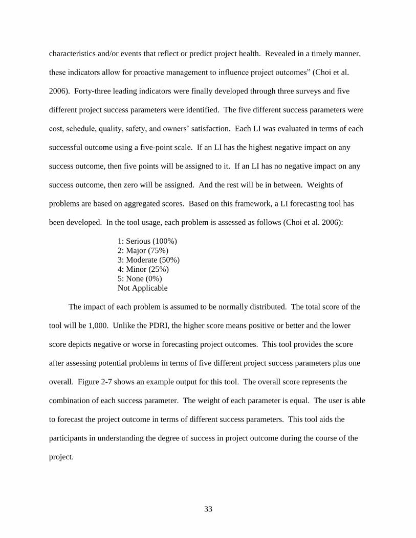
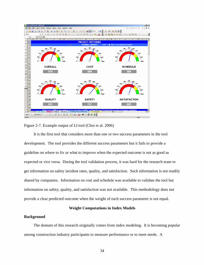
The impact of each problem is assumed to be normally distributed. The total score of the
tool will be 1,000. Unlike the PDRI, the higher score means positive or better and the lower
score depicts negative or worse in forecasting project outcomes. This tool provides the score
after assessing potential problems in terms of five different project success parameters plus one
overall. Figure 2-7 shows an example output for this tool. The overall score represents the
combination of each success parameter. The weight of each parameter is equal. The user is able
to forecast the project outcome in terms of different success parameters. This tool aids the
participants in understanding the degree of success in project outcome during the course of the
project.
34
Figure 2-7. Example output of LI tool (Choi et al. 2006)
It is the first tool that considers more than one or two success parameters in the tool
development. The tool provides the different success parameters but it fails to provide a
guideline on where to fix or what to improve when the expected outcome is not as good as
expected or vice versa. During the tool validation process, it was hard for the research team to
get information on safety incident rates, quality, and satisfaction. Such information is not readily
shared by companies. Information on cost and schedule was available to validate the tool but
information on safety, quality, and satisfaction was not available. This methodology does not
provide a clear predicted outcome when the weight of each success parameter is not equal.
Weight Computations in Index Models
Background
The domain of this research originally comes from index modeling. It is becoming popular
among construction industry participants to measure performance or to meet needs. A
35
construction company will develop an index model to meet their owners‟ expectations and
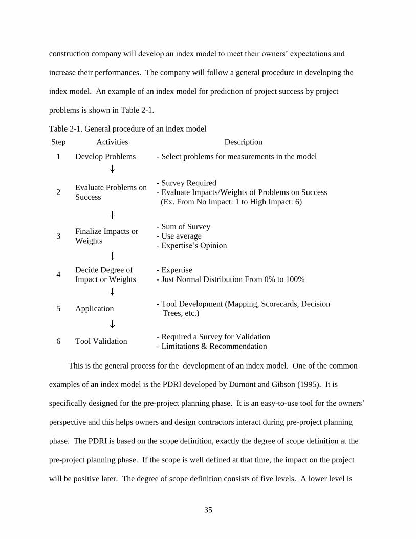
increase their performances. The company will follow a general procedure in developing the
index model. An example of an index model for prediction of project success by project
problems is shown in Table 2-1.
Table 2-1. General procedure of an index model
Step Activities Description
1 Develop Problems - Select problems for measurements in the model
2 Evaluate Problems on
Success
- Survey Required
- Evaluate Impacts/Weights of Problems on Success
(Ex. From No Impact: 1 to High Impact: 6)
3 Finalize Impacts or
Weights
- Sum of Survey
- Use average
- Expertise‟s Opinion
4 Decide Degree of
Impact or Weights
- Expertise
- Just Normal Distribution From 0% to 100%
5 Application - Tool Development (Mapping, Scorecards, Decision
Trees, etc.)
6 Tool Validation - Required a Survey for Validation
- Limitations & Recommendation
This is the general process for the development of an index model. One of the common
examples of an index model is the PDRI developed by Dumont and Gibson (1995). It is
specifically designed for the pre-project planning phase. It is an easy-to-use tool for the owners‟
perspective and this helps owners and design contractors interact during pre-project planning
phase. The PDRI is based on the scope definition, exactly the degree of scope definition at the
pre-project planning phase. If the scope is well defined at that time, the impact on the project
will be positive later. The degree of scope definition consists of five levels. A lower level is
36
better than a higher level for the project scope definition. All elements are weighted by level of
scope definitions and there is no limit on weighing. Weighing point represents that each
element‟s impact on TIC stated as a percentage of the overall estimate. Therefore the lower
points, the better project scope definition is. Finally all the data are normalized by 1,000 scale
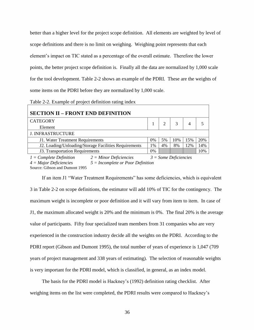
for the tool development. Table 2-2 shows an example of the PDRI. These are the weights of
some items on the PDRI before they are normalized by 1,000 scale.
Table 2-2. Example of project definition rating index
SECTION II – FRONT END DEFINITION
CATEGORY 1 2 3 4 5
Element
J. INFRASTRUCTURE
J1. Water Treatment Requirements 0% 5% 10% 15% 20%
J2. Loading/Unloading/Storage Facilities Requirements 1% 4% 8% 12% 14%
J3. Transportation Requirements 0% 10%
1 = Complete Definition 2 = Minor Deficiencies 3 = Some Deficiencies
4 = Major Deficiencies 5 = Incomplete or Poor Definition Source: Gibson and Dumont 1995
If an item J1 “Water Treatment Requirements” has some deficiencies, which is equivalent
3 in Table 2-2 on scope definitions, the estimator will add 10% of TIC for the contingency. The
maximum weight is incomplete or poor definition and it will vary from item to item. In case of
J1, the maximum allocated weight is 20% and the minimum is 0%. The final 20% is the average
value of participants. Fifty four specialized team members from 31 companies who are very
experienced in the construction industry decide all the weights on the PDRI. According to the
PDRI report (Gibson and Dumont 1995), the total number of years of experience is 1,047 (709
years of project management and 338 years of estimating). The selection of reasonable weights
is very important for the PDRI model, which is classified, in general, as an index model.
The basis for the PDRI model is Hackney‟s (1992) definition rating checklist. After
weighing items on the list were completed, the PDRI results were compared to Hackney‟s
37
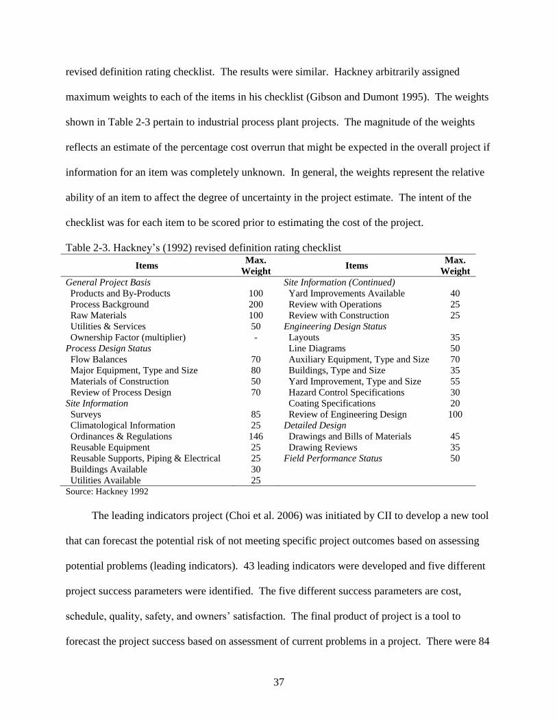
revised definition rating checklist. The results were similar. Hackney arbitrarily assigned
maximum weights to each of the items in his checklist (Gibson and Dumont 1995). The weights
shown in Table 2-3 pertain to industrial process plant projects. The magnitude of the weights
reflects an estimate of the percentage cost overrun that might be expected in the overall project if
information for an item was completely unknown. In general, the weights represent the relative
ability of an item to affect the degree of uncertainty in the project estimate. The intent of the
checklist was for each item to be scored prior to estimating the cost of the project.
Table 2-3. Hackney‟s (1992) revised definition rating checklist
Items Max.
Weight Items
Max.
Weight
General Project Basis Site Information (Continued)
Products and By-Products 100 Yard Improvements Available 40
Process Background 200 Review with Operations 25
Raw Materials 100 Review with Construction 25
Utilities & Services 50 Engineering Design Status
Ownership Factor (multiplier) - Layouts 35
Process Design Status Line Diagrams 50
Flow Balances 70 Auxiliary Equipment, Type and Size 70
Major Equipment, Type and Size 80 Buildings, Type and Size 35
Materials of Construction 50 Yard Improvement, Type and Size 55
Review of Process Design 70 Hazard Control Specifications 30
Site Information Coating Specifications 20
Surveys 85 Review of Engineering Design 100
Climatological Information 25 Detailed Design
Ordinances & Regulations 146 Drawings and Bills of Materials 45
Reusable Equipment 25 Drawing Reviews 35
Reusable Supports, Piping & Electrical 25 Field Performance Status 50
Buildings Available 30
Utilities Available 25
Source: Hackney 1992
The leading indicators project (Choi et al. 2006) was initiated by CII to develop a new tool
that can forecast the potential risk of not meeting specific project outcomes based on assessing
potential problems (leading indicators). 43 leading indicators were developed and five different
project success parameters were identified. The five different success parameters are cost,
schedule, quality, safety, and owners‟ satisfaction. The final product of project is a tool to
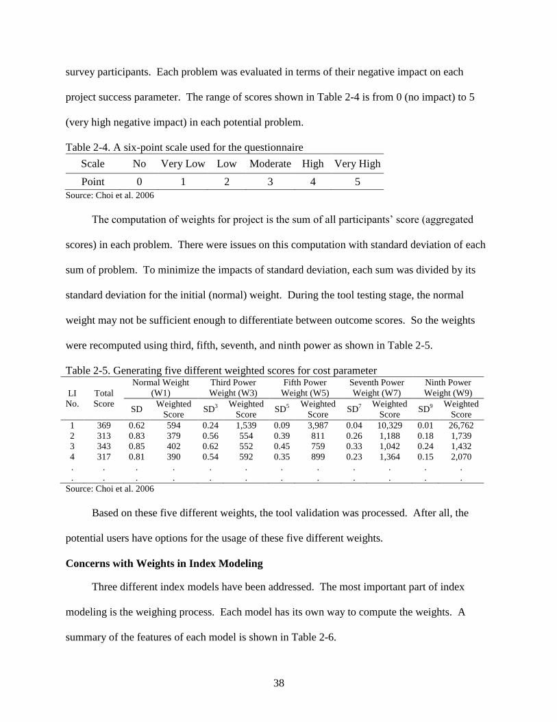
forecast the project success based on assessment of current problems in a project. There were 84
38
survey participants. Each problem was evaluated in terms of their negative impact on each
project success parameter. The range of scores shown in Table 2-4 is from 0 (no impact) to 5
(very high negative impact) in each potential problem.
Table 2-4. A six-point scale used for the questionnaire
Scale No Very Low Low Moderate High Very High
Point 0 1 2 3 4 5
Source: Choi et al. 2006
The computation of weights for project is the sum of all participants‟ score (aggregated
scores) in each problem. There were issues on this computation with standard deviation of each
sum of problem. To minimize the impacts of standard deviation, each sum was divided by its
standard deviation for the initial (normal) weight. During the tool testing stage, the normal
weight may not be sufficient enough to differentiate between outcome scores. So the weights
were recomputed using third, fifth, seventh, and ninth power as shown in Table 2-5.
Table 2-5. Generating five different weighted scores for cost parameter
LI
No.
Total
Score
Normal Weight
(W1)
Third Power
Weight (W3)
Fifth Power
Weight (W5)
Seventh Power
Weight (W7)
Ninth Power
Weight (W9)
SD Weighted
Score SD
3
Weighted
Score SD
5
Weighted
Score SD
7
Weighted
Score SD
9
Weighted
Score
1 369 0.62 594 0.24 1,539 0.09 3,987 0.04 10,329 0.01 26,762
2 313 0.83 379 0.56 554 0.39 811 0.26 1,188 0.18 1,739
3 343 0.85 402 0.62 552 0.45 759 0.33 1,042 0.24 1,432
4 317 0.81 390 0.54 592 0.35 899 0.23 1,364 0.15 2,070
.
.
.
.
.
.
.
.
.
.
.
.
.
.
.
.
.
.
.
.
.
.
.
.
Source: Choi et al. 2006
Based on these five different weights, the tool validation was processed. After all, the
potential users have options for the usage of these five different weights.
Concerns with Weights in Index Modeling
Three different index models have been addressed. The most important part of index
modeling is the weighing process. Each model has its own way to compute the weights. A
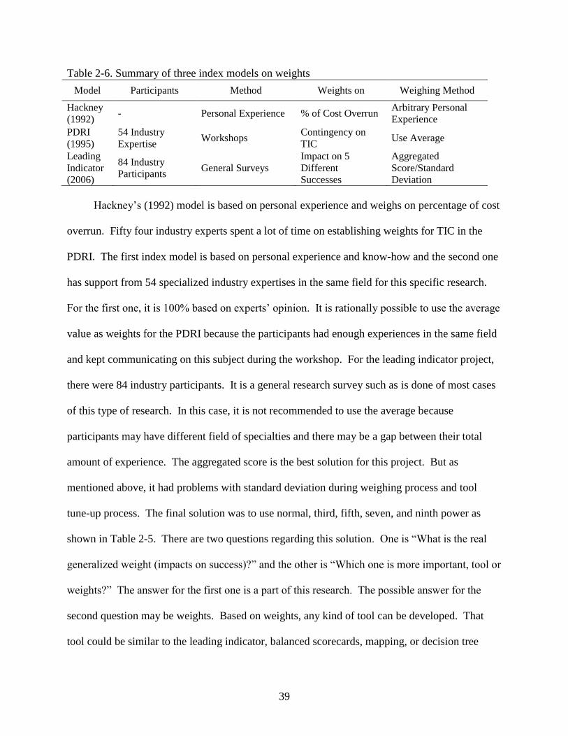
summary of the features of each model is shown in Table 2-6.
39
Table 2-6. Summary of three index models on weights
Model Participants Method Weights on Weighing Method
Hackney
(1992) - Personal Experience % of Cost Overrun
Arbitrary Personal
Experience
PDRI
(1995)
54 Industry
Expertise Workshops
Contingency on
TIC Use Average
Leading
Indicator
(2006)
84 Industry
Participants General Surveys
Impact on 5
Different
Successes
Aggregated
Score/Standard
Deviation
Hackney‟s (1992) model is based on personal experience and weighs on percentage of cost
overrun. Fifty four industry experts spent a lot of time on establishing weights for TIC in the
PDRI. The first index model is based on personal experience and know-how and the second one
has support from 54 specialized industry expertises in the same field for this specific research.
For the first one, it is 100% based on experts‟ opinion. It is rationally possible to use the average
value as weights for the PDRI because the participants had enough experiences in the same field
and kept communicating on this subject during the workshop. For the leading indicator project,
there were 84 industry participants. It is a general research survey such as is done of most cases
of this type of research. In this case, it is not recommended to use the average because
participants may have different field of specialties and there may be a gap between their total
amount of experience. The aggregated score is the best solution for this project. But as
mentioned above, it had problems with standard deviation during weighing process and tool
tune-up process. The final solution was to use normal, third, fifth, seven, and ninth power as
shown in Table 2-5. There are two questions regarding this solution. One is “What is the real
generalized weight (impacts on success)?” and the other is “Which one is more important, tool or
weights?” The answer for the first one is a part of this research. The possible answer for the
second question may be weights. Based on weights, any kind of tool can be developed. That
tool could be similar to the leading indicator, balanced scorecards, mapping, or decision tree
40
tools. The answer to the second question may be controversial. But the importance of weight in
the index model is extremely high.
What Hackney (1992) and the PDRI model measure is tangible costs and schedule
durations. That is why both used percentage as weights. Problems and items on the checklist
were developed for these two measures. There is a demand for new project success parameters.
Cost and schedule are the most traditional common project success parameters. But there are
some more parameters that impact the success of projects, e.g. safety, quality, and owner‟s
satisfaction. The first two models are designed mainly for cost and schedule but the leading
indicator project is designed for five different success parameters. The five success parameters
are cost, schedule, quality, safety, and satisfaction. Two of these parameters could be tangible
like cost and schedule but the rest of parameters cannot be tangible. The leading indicator
project has to be consistent in measuring the impacts of each success parameter. A project
should not have more than one method to measure something. For example, the contingency (%)
for cost and schedule and degrees of impact for quality, safety, and satisfaction may not be a
good solution for weight. In the opinion of this author, one of the main reasons to use different
powers in the leading indicator project is the range of evaluation is too narrow so that aggregated
scores did not make any big difference at the end. But if a wider range of impacts had been used,
the aggregated scores could have made a bigger difference and then the standard deviation could
have been larger as well. The range of impacts or measurements is optimal between five and
nine (Spector 1992). So the evaluation method of a problem‟s impact on each success parameter
shown in Table 2-4 is reasonable. Users could not tell the degree of differences over this range
in the survey. The first two models, Hackney‟s and the PDRI could be considered as special
cases and the last model, the leading indicator, could be considered as a general case from
41
surveys to tool validation process. From this perspective, there are some concerns with weight
and their method of computation no matter what the specialized area is in the index modeling.
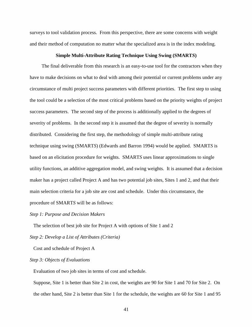
Simple Multi-Attribute Rating Technique Using Swing (SMARTS)
The final deliverable from this research is an easy-to-use tool for the contractors when they
have to make decisions on what to deal with among their potential or current problems under any
circumstance of multi project success parameters with different priorities. The first step to using
the tool could be a selection of the most critical problems based on the priority weights of project
success parameters. The second step of the process is additionally applied to the degrees of
severity of problems. In the second step it is assumed that the degree of severity is normally
distributed. Considering the first step, the methodology of simple multi-attribute rating
technique using swing (SMARTS) (Edwards and Barron 1994) would be applied. SMARTS is
based on an elicitation procedure for weights. SMARTS uses linear approximations to single
utility functions, an additive aggregation model, and swing weights. It is assumed that a decision
maker has a project called Project A and has two potential job sites, Sites 1 and 2, and that their
main selection criteria for a job site are cost and schedule. Under this circumstance, the
procedure of SMARTS will be as follows:
Step 1: Purpose and Decision Makers
The selection of best job site for Project A with options of Site 1 and 2
Step 2: Develop a List of Attributes (Criteria)
Cost and schedule of Project A
Step 3: Objects of Evaluations
Evaluation of two job sites in terms of cost and schedule.
Suppose, Site 1 is better than Site 2 in cost, the weights are 90 for Site 1 and 70 for Site 2. On
the other hand, Site 2 is better than Site 1 for the schedule, the weights are 60 for Site 1 and 95
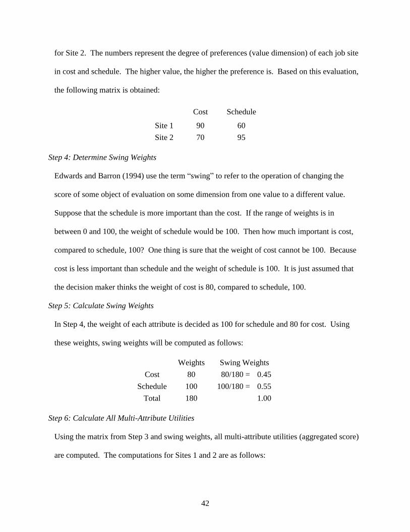
42
for Site 2. The numbers represent the degree of preferences (value dimension) of each job site
in cost and schedule. The higher value, the higher the preference is. Based on this evaluation,
the following matrix is obtained:
Cost Schedule
Site 1 90 60
Site 2 70 95
Step 4: Determine Swing Weights
Edwards and Barron (1994) use the term “swing” to refer to the operation of changing the
score of some object of evaluation on some dimension from one value to a different value.
Suppose that the schedule is more important than the cost. If the range of weights is in
between 0 and 100, the weight of schedule would be 100. Then how much important is cost,
compared to schedule, 100? One thing is sure that the weight of cost cannot be 100. Because
cost is less important than schedule and the weight of schedule is 100. It is just assumed that
the decision maker thinks the weight of cost is 80, compared to schedule, 100.
Step 5: Calculate Swing Weights
In Step 4, the weight of each attribute is decided as 100 for schedule and 80 for cost. Using
these weights, swing weights will be computed as follows:
Weights Swing Weights
Cost 80 80/180 = 0.45
Schedule 100 100/180 = 0.55
Total 180 1.00
Step 6: Calculate All Multi-Attribute Utilities
Using the matrix from Step 3 and swing weights, all multi-attribute utilities (aggregated score)
are computed. The computations for Sites 1 and 2 are as follows:
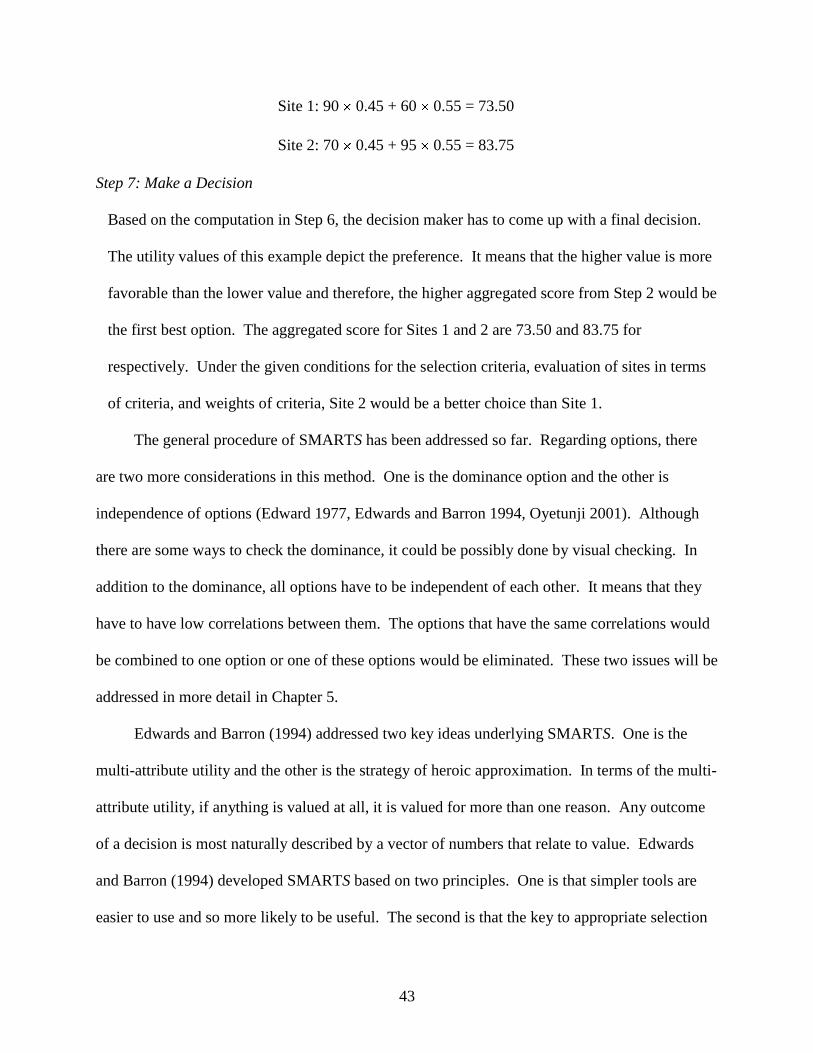
43
Site 1: 90 0.45 + 60 0.55 = 73.50
Site 2: 70 0.45 + 95 0.55 = 83.75
Step 7: Make a Decision
Based on the computation in Step 6, the decision maker has to come up with a final decision.
The utility values of this example depict the preference. It means that the higher value is more
favorable than the lower value and therefore, the higher aggregated score from Step 2 would be
the first best option. The aggregated score for Sites 1 and 2 are 73.50 and 83.75 for
respectively. Under the given conditions for the selection criteria, evaluation of sites in terms
of criteria, and weights of criteria, Site 2 would be a better choice than Site 1.
The general procedure of SMARTS has been addressed so far. Regarding options, there
are two more considerations in this method. One is the dominance option and the other is
independence of options (Edward 1977, Edwards and Barron 1994, Oyetunji 2001). Although
there are some ways to check the dominance, it could be possibly done by visual checking. In
addition to the dominance, all options have to be independent of each other. It means that they
have to have low correlations between them. The options that have the same correlations would
be combined to one option or one of these options would be eliminated. These two issues will be
addressed in more detail in Chapter 5.
Edwards and Barron (1994) addressed two key ideas underlying SMARTS. One is the
multi-attribute utility and the other is the strategy of heroic approximation. In terms of the multi-
attribute utility, if anything is valued at all, it is valued for more than one reason. Any outcome
of a decision is most naturally described by a vector of numbers that relate to value. Edwards
and Barron (1994) developed SMARTS based on two principles. One is that simpler tools are
easier to use and so more likely to be useful. The second is that the key to appropriate selection
44
of methods is concern about the trade-off between modeling error and elicitation error. In its
previous version, SMART, included the judgments of the indifference between pairs of
hypothetical options which seemed difficult and unstable. The authors believed that more nearly
direct assessments of the desired quantities were easier and less likely to produce elicitation
errors and call that view the strategy of heroic approximation. Users of that strategy do not
identify formally justifiable judgments and then figure out how to elicit them. Rather they
identify the simplest possible judgments that have any hope of meeting the underlying
requirements of multi-attribute utility measurement, and try to determine whether they will lead
to substantially suboptimal choices in the problem at hand. If not, they try to avoid elicitation
errors by using those methods.
In this chapter, the literature review for this research has been presented in terms of its
relevance to the research. The first part of this chapter addresses the major factors and/or
problems of projects. The major issue is to define factors and/or problems without their impacts
on projects. Another part focuses on the current trends or research of how to measure project
performances and its usage as a tool or index model in terms of project success parameters. This
section clearly shows the current research needs in this area for some more work on multi-project
success parameters and their relationships with problems. In other words, the current research
focuses on a single or two success parameters. The last part of this section addresses some
considerations on weight computation and a methodology for the application.
45
CHAPTER 3
STRATEGY AND DESIGN
Overview
This chapter will mainly address the overall strategy and design of this research. This
includes the data collection, the methodologies for this research such as canonical correlations
and factor analysis (exploratory factor analysis and confirmatory factor analysis). Regarding
data collection, the background for the data collection will be discussed. Canonical correlations
will address concepts and how it relates to this research and their outputs. The concepts of
exploratory factor analysis (EFA) and confirmatory factor analysis (CFA) will also be addressed.
Development of Problems
All the necessary data were obtained from the leading indicators project (Choi et al. 2006).
It developed 43 potential problems with five project outcomes (success parameters). The 43
problems are listed in Appendix A. The defined five success parameters by the research team
were 1) Cost; 2) Schedule; 3) Quality/Operability (Quality); 4) Safety; and 5) Stakeholder
satisfaction. These five parameters are generally and traditionally used to measure project
success in many industries. The definitions for each parameter are as follows (Choi et al. 2006):
Cost: Cost performance is viewed in terms of overall actual final cost versus the
established project budget. Secondary cost outcomes can include cost/cash flow deviation
(compliance with spending plans), cost efficiency (how efficiently an asset is design and
constructed verses similar facilities in industry), and consumption of contingency or
reserves.
Schedule: Schedule performance is viewed in terms of overall actual final duration versus
the planned project duration. Secondary schedule performance can include outage duration
performances and overall engineering and construction cycle time (for certain fast rack
projects).
Quality/Operability: Quality and Operability are outcomes that are based upon a facility
being capable of operating per its intended function and that the quality of the facility and
construction craftsmanship matches the intended asset lift. (For example, if we build a
facility that is intended to make 100 widgets a day, the facility should be capable of making
100 widgets a day).
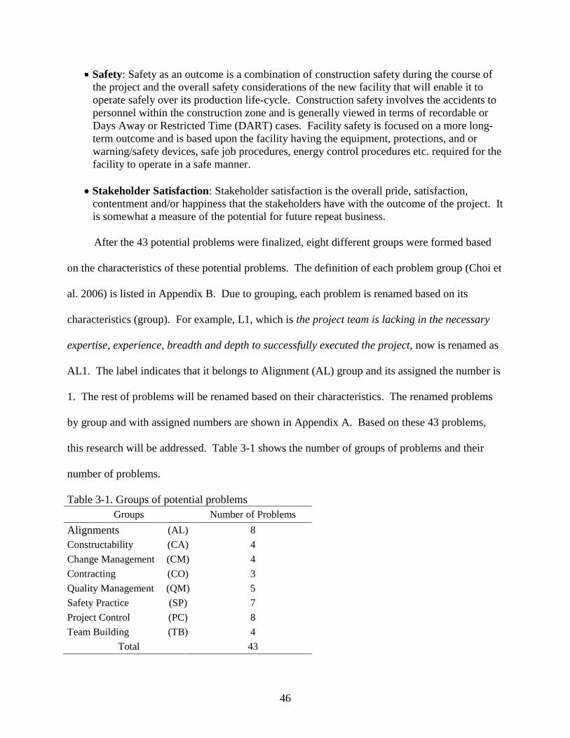
46
Safety: Safety as an outcome is a combination of construction safety during the course of
the project and the overall safety considerations of the new facility that will enable it to
operate safely over its production life-cycle. Construction safety involves the accidents to
personnel within the construction zone and is generally viewed in terms of recordable or
Days Away or Restricted Time (DART) cases. Facility safety is focused on a more long-
term outcome and is based upon the facility having the equipment, protections, and or
warning/safety devices, safe job procedures, energy control procedures etc. required for the
facility to operate in a safe manner.
Stakeholder Satisfaction: Stakeholder satisfaction is the overall pride, satisfaction,
contentment and/or happiness that the stakeholders have with the outcome of the project. It
is somewhat a measure of the potential for future repeat business.
After the 43 potential problems were finalized, eight different groups were formed based
on the characteristics of these potential problems. The definition of each problem group (Choi et
al. 2006) is listed in Appendix B. Due to grouping, each problem is renamed based on its
characteristics (group). For example, L1, which is the project team is lacking in the necessary
expertise, experience, breadth and depth to successfully executed the project, now is renamed as
AL1. The label indicates that it belongs to Alignment (AL) group and its assigned the number is
1. The rest of problems will be renamed based on their characteristics. The renamed problems
by group and with assigned numbers are shown in Appendix A. Based on these 43 problems,
this research will be addressed. Table 3-1 shows the number of groups of problems and their
number of problems.
Table 3-1. Groups of potential problems
Groups Number of Problems
Alignments (AL) 8
Constructability (CA) 4
Change Management (CM) 4
Contracting (CO) 3
Quality Management (QM) 5
Safety Practice (SP) 7
Project Control (PC) 8
Team Building (TB) 4
Total 43
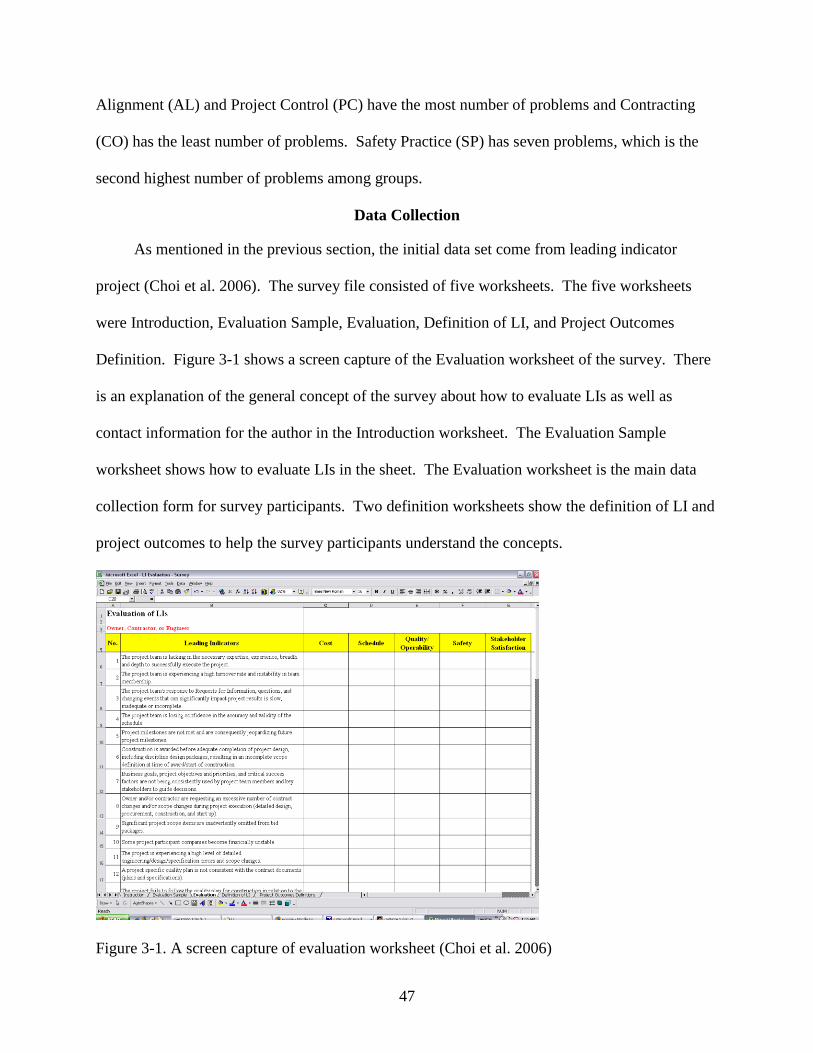
47
Alignment (AL) and Project Control (PC) have the most number of problems and Contracting
(CO) has the least number of problems. Safety Practice (SP) has seven problems, which is the
second highest number of problems among groups.
Data Collection
As mentioned in the previous section, the initial data set come from leading indicator
project (Choi et al. 2006). The survey file consisted of five worksheets. The five worksheets
were Introduction, Evaluation Sample, Evaluation, Definition of LI, and Project Outcomes
Definition. Figure 3-1 shows a screen capture of the Evaluation worksheet of the survey. There
is an explanation of the general concept of the survey about how to evaluate LIs as well as
contact information for the author in the Introduction worksheet. The Evaluation Sample
worksheet shows how to evaluate LIs in the sheet. The Evaluation worksheet is the main data
collection form for survey participants. Two definition worksheets show the definition of LI and
project outcomes to help the survey participants understand the concepts.
Figure 3-1. A screen capture of evaluation worksheet (Choi et al. 2006)
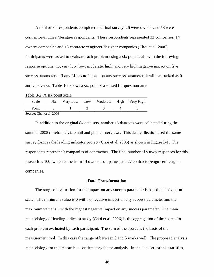
48
A total of 84 respondents completed the final survey: 26 were owners and 58 were
contractor/engineer/designer respondents. These respondents represented 32 companies: 14
owners companies and 18 contractor/engineer/designer companies (Choi et al. 2006).
Participants were asked to evaluate each problem using a six point scale with the following
response options: no, very low, low, moderate, high, and very high negative impact on five
success parameters. If any LI has no impact on any success parameter, it will be marked as 0
and vice versa. Table 3-2 shows a six point scale used for questionnaire.
Table 3-2. A six point scale
Scale No Very Low Low Moderate High Very High
Point 0 1 2 3 4 5
Source: Choi et al. 2006
In addition to the original 84 data sets, another 16 data sets were collected during the
summer 2008 timeframe via email and phone interviews. This data collection used the same
survey form as the leading indicator project (Choi et al. 2006) as shown in Figure 3-1. The
respondents represent 9 companies of contractors. The final number of survey responses for this
research is 100, which came from 14 owners companies and 27 contractor/engineer/designer
companies.
Data Transformation
The range of evaluation for the impact on any success parameter is based on a six point
scale. The minimum value is 0 with no negative impact on any success parameter and the
maximum value is 5 with the highest negative impact on any success parameter. The main
methodology of leading indicator study (Choi et al. 2006) is the aggregation of the scores for
each problem evaluated by each participant. The sum of the scores is the basis of the
measurement tool. In this case the range of between 0 and 5 works well. The proposed analysis
methodology for this research is confirmatory factor analysis. In the data set for this statistics,
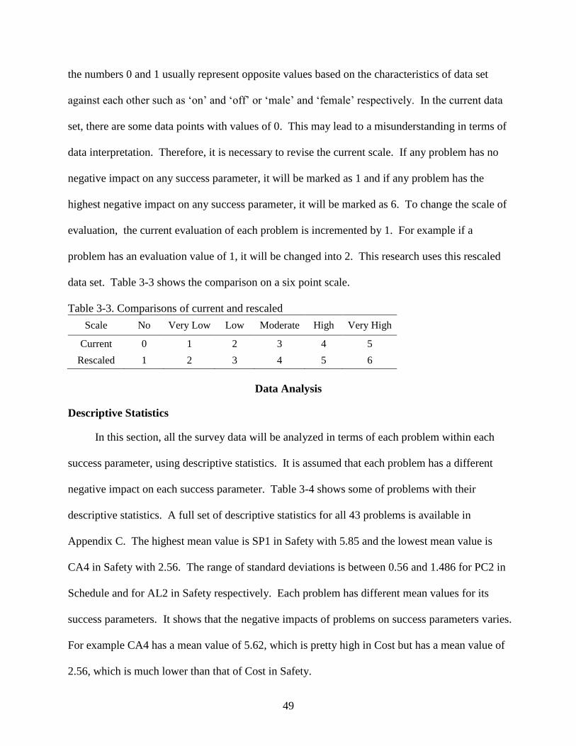
49
the numbers 0 and 1 usually represent opposite values based on the characteristics of data set
against each other such as „on‟ and „off‟ or „male‟ and „female‟ respectively. In the current data
set, there are some data points with values of 0. This may lead to a misunderstanding in terms of
data interpretation. Therefore, it is necessary to revise the current scale. If any problem has no
negative impact on any success parameter, it will be marked as 1 and if any problem has the
highest negative impact on any success parameter, it will be marked as 6. To change the scale of
evaluation, the current evaluation of each problem is incremented by 1. For example if a
problem has an evaluation value of 1, it will be changed into 2. This research uses this rescaled
data set. Table 3-3 shows the comparison on a six point scale.
Table 3-3. Comparisons of current and rescaled
Scale No Very Low Low Moderate High Very High
Current 0 1 2 3 4 5
Rescaled 1 2 3 4 5 6
Data Analysis
Descriptive Statistics
In this section, all the survey data will be analyzed in terms of each problem within each
success parameter, using descriptive statistics. It is assumed that each problem has a different
negative impact on each success parameter. Table 3-4 shows some of problems with their
descriptive statistics. A full set of descriptive statistics for all 43 problems is available in
Appendix C. The highest mean value is SP1 in Safety with 5.85 and the lowest mean value is
CA4 in Safety with 2.56. The range of standard deviations is between 0.56 and 1.486 for PC2 in
Schedule and for AL2 in Safety respectively. Each problem has different mean values for its
success parameters. It shows that the negative impacts of problems on success parameters varies.
For example CA4 has a mean value of 5.62, which is pretty high in Cost but has a mean value of
2.56, which is much lower than that of Cost in Safety.
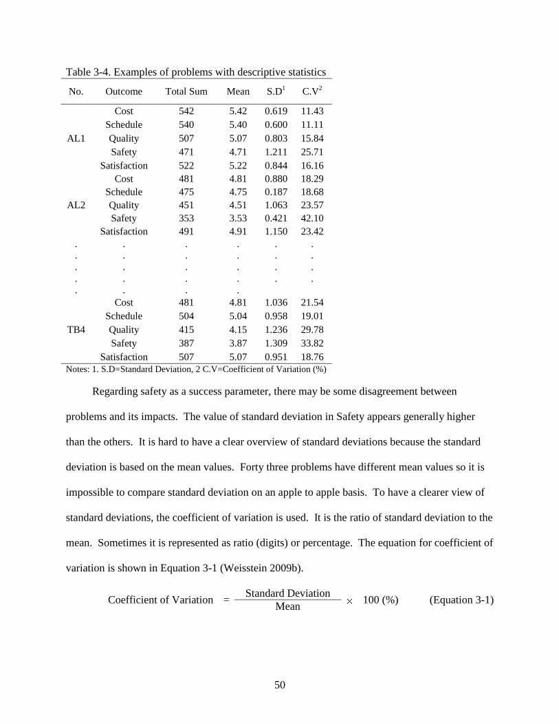
50
Table 3-4. Examples of problems with descriptive statistics
No. Outcome Total Sum Mean S.D1 C.V
2
AL1
Cost 542 5.42 0.619 11.43
Schedule 540 5.40 0.600 11.11
Quality 507 5.07 0.803 15.84
Safety 471 4.71 1.211 25.71
Satisfaction 522 5.22 0.844 16.16
AL2
Cost 481 4.81 0.880 18.29
Schedule 475 4.75 0.187 18.68
Quality 451 4.51 1.063 23.57
Safety 353 3.53 0.421 42.10
Satisfaction 491 4.91 1.150 23.42
.
.
.
.
.
.
.
.
.
.
.
.
.
.
.
.
.
.
.
.
.
.
.
.
.
.
.
.
TB4
Cost 481 4.81 1.036 21.54
Schedule 504 5.04 0.958 19.01
Quality 415 4.15 1.236 29.78
Safety 387 3.87 1.309 33.82
Satisfaction 507 5.07 0.951 18.76
Notes: 1. S.D=Standard Deviation, 2 C.V=Coefficient of Variation (%)
Regarding safety as a success parameter, there may be some disagreement between
problems and its impacts. The value of standard deviation in Safety appears generally higher
than the others. It is hard to have a clear overview of standard deviations because the standard
deviation is based on the mean values. Forty three problems have different mean values so it is
impossible to compare standard deviation on an apple to apple basis. To have a clearer view of
standard deviations, the coefficient of variation is used. It is the ratio of standard deviation to the
mean. Sometimes it is represented as ratio (digits) or percentage. The equation for coefficient of
variation is shown in Equation 3-1 (Weisstein 2009b).
Coefficient of Variation = Standard Deviation
100 (%) (Equation 3-1) Mean
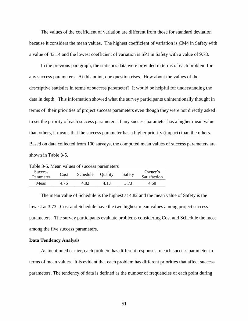
51
The values of the coefficient of variation are different from those for standard deviation
because it considers the mean values. The highest coefficient of variation is CM4 in Safety with
a value of 43.14 and the lowest coefficient of variation is SP1 in Safety with a value of 9.78.
In the previous paragraph, the statistics data were provided in terms of each problem for
any success parameters. At this point, one question rises. How about the values of the
descriptive statistics in terms of success parameter? It would be helpful for understanding the
data in depth. This information showed what the survey participants unintentionally thought in
terms of their priorities of project success parameters even though they were not directly asked
to set the priority of each success parameter. If any success parameter has a higher mean value
than others, it means that the success parameter has a higher priority (impact) than the others.
Based on data collected from 100 surveys, the computed mean values of success parameters are
shown in Table 3-5.
Table 3-5. Mean values of success parameters Success
Parameter Cost Schedule Quality Safety
Owner‟s
Satisfaction
Mean 4.76 4.82 4.13 3.73 4.68
The mean value of Schedule is the highest at 4.82 and the mean value of Safety is the
lowest at 3.73. Cost and Schedule have the two highest mean values among project success
parameters. The survey participants evaluate problems considering Cost and Schedule the most
among the five success parameters.
Data Tendency Analysis
As mentioned earlier, each problem has different responses to each success parameter in
terms of mean values. It is evident that each problem has different priorities that affect success
parameters. The tendency of data is defined as the number of frequencies of each point during
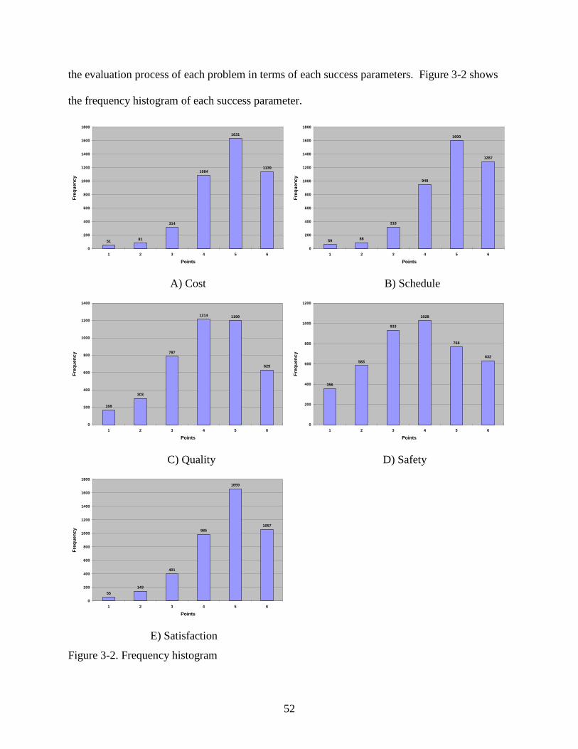
52
the evaluation process of each problem in terms of each success parameters. Figure 3-2 shows
the frequency histogram of each success parameter.
5181
314
1084
1631
1139
0
200
400
600
800
1000
1200
1400
1600
1800
1 2 3 4 5 6
Points
Fre
qu
en
cy
5988
318
948
1600
1287
0
200
400
600
800
1000
1200
1400
1600
1800
1 2 3 4 5 6
Points
Fre
qu
en
cy
A) Cost B) Schedule
168
303
787
1214 1199
629
0
200
400
600
800
1000
1200
1400
1 2 3 4 5 6
Points
Fre
qu
en
cy
356
583
933
1028
768
632
0
200
400
600
800
1000
1200
1 2 3 4 5 6
Points
Fre
qu
en
cy
C) Quality D) Safety
55
143
401
985
1659
1057
0
200
400
600
800
1000
1200
1400
1600
1800
1 2 3 4 5 6
Points
Fre
qu
en
cy
E) Satisfaction
Figure 3-2. Frequency histogram
53
Regarding data tendency, cost, schedule, and satisfaction have the similar tendency as
shown in Figures 3-2 A, B, and E. Quality and safety show similar tendency as shown in
Figures 3-2 C and D. The frequency histograms of cost, schedule, and satisfaction are skewed to
the left and the frequency histograms of quality and safety look like they are normally distributed.
It shows that the cost, schedule, and satisfaction groups have more problems with a value of 5 or
greater than those of the group of quality and safety. The two most frequent values are 5 and 6
for Cost, Schedule, and Satisfaction and 4 and 5 for Quality and Safety.
From the descriptive statistics and frequency histograms, we can conclude that there are
two main characteristics of data. One is that each problem has a different response to any
success parameters and the other is that each success parameter has a different priority. There
are no problems that always have the highest score or lowest score to all five success parameters.
It is apparent that problems‟ responses to success parameter are dynamic. In addition to this, the
frequency of values over 5 in Cost, Schedule, and Satisfaction are higher than those for Quality
and Safety.
Methodology
Background
The data available for this research are for 43 potential problems with 8 groups of
parameters. The input data mainly are provided by industrial project companies so it may not be
suitable for other types of construction projects such as commercial, residential, and heavy civil.
It is important to understand the relationships within each success parameter before identifying a
relationship between problems and success parameter. To define the relationships between
variables (problems), there are several statistical methods (techniques) available to define the
relationships between variables such as 1) correlations, 2) multiple regression, 3) factor analysis,
and 4) canonical correlations. Regarding the methodology for the analysis of relationships
54
between problem groups and success parameters, SMARTS will not be mentioned in this chapter
because it was already addressed in Chapter 2.
Correlations show the strength and direction of a linear relationship between two variables.
It could be ideal for this data analysis. But there are 43 variables for this research and it means
the generated matrix will be a matrix of 43 43. Since 43 variables are grouped by their
characteristics, it would be better comparing group to group not a variable to variable.
Correlation does not allow for group-to-group analysis, hence it is not recommended for this data
analysis. Multiple regression consists of one set of dependent (criterion) variables and more than
two sets of independent (predictor) variables. It will provide one linear combination of
dependent and independent variables. One of the main purposes of multiple regressions is to
develop a prediction model. For the purposes of this study multiple regression is not required.
Factor analysis is commonly used to determine the number of “factors” being measured by a
variable. The main function of this method is to determine the underlying factor(s) and data
reduction. There are two types of methods in this analysis. They are exploratory factor analysis
(EFA) and confirmatory factor analysis (CFA). Regarding confirmatory factor analysis, it will
be addressed later in this study. The data has been grouped as eight different groups. It is not
necessary to perform factor analysis to determine factors for this research but is necessary to
check how many factors would be extracted before performing CFA. Canonical correlations
show the relationships between two variable sets. Each set has more than two variables. Unlike
multiple regressions, canonical correlations generate two linear combinations, one for criterion
and the other for predictor. This is the main difference between multiple regression and
canonical correlations. Canonical correlation provides the maximum correlations between two
sets. It is suitable for this research to define relationships between groups of multiple variables.
55
Canonical Correlation
Overview
Canonical correlation analysis is used to explore relationships between two variable sets
when each variable set has at least two variables (Thompson 1984). One variable set represents
independent variables and the other variable set represents dependent variables. “The canonical
correlation is optimized such that the linear correlation between two latent variables is
maximized. Whereas multiple regressions is used for many-to-one relationships, canonical
correlation is used for many-to-many relationships (Garson 2008a). ” Due to many-to-many
relationships, it is possible to have more than one correlation relating two sets of variables. A
total number of possible correlations are set by a number of smaller variable sets. For example,
if there are two variable sets available which are a set of three variables and another set of five
variables, then the number of possible correlations between these two sets is three. With respect
to the characteristics of computation of correlations, the first extracted correlation usually has the
highest value and the last correlation has the lowest value. To test the significance of canonical
correlation, Wilk‟s lambda is commonly used. Some of key concepts and terms are as follows
(Garson 2008a):
“Canonical variate: A canonical variate is a linear combination of a set of original variables
in which the within-set correlation has been controlled. There are two canonical variates
per canonical correlation. One is the dependent canonical variable, while the one for the
independent variables may be called the covariate canonical variable.”
“Canonical correlation: A canonical correlation, also called a characteristic root, is a form
of correlation relating two sets of variables. As with factor analysis, there may be more
than one significant dimension (more than one canonical correlation), each representing an
orthogonally separate pattern of relationships between the two latent variables.”
“Eigenvalues: The Eigenvalues are approximately equal to the canonical correlations
squared. They reflect the proportion of variance in the canonical variate explained by the
canonical correlation relating two sets of variables. This is only useful when there is more
than one extracted canonical correlation and more than one Eigenvalue, one for each
canonical correlation.”
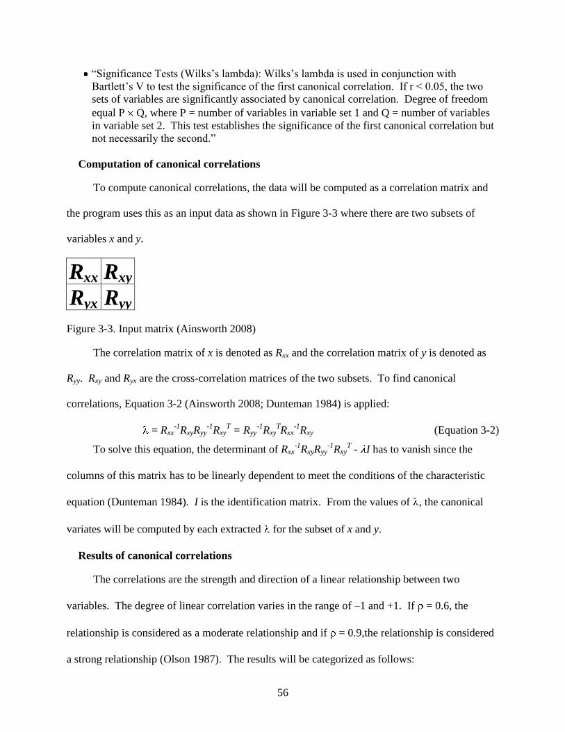
56
“Significance Tests (Wilks‟s lambda): Wilks‟s lambda is used in conjunction with
Bartlett‟s V to test the significance of the first canonical correlation. If r < 0.05, the two
sets of variables are significantly associated by canonical correlation. Degree of freedom
equal P Q, where P = number of variables in variable set 1 and Q = number of variables
in variable set 2. This test establishes the significance of the first canonical correlation but
not necessarily the second.”
Computation of canonical correlations
To compute canonical correlations, the data will be computed as a correlation matrix and
the program uses this as an input data as shown in Figure 3-3 where there are two subsets of
variables x and y.
Rxx Rxy
Ryx Ryy
Figure 3-3. Input matrix (Ainsworth 2008)
The correlation matrix of x is denoted as Rxx and the correlation matrix of y is denoted as
Ryy. Rxy and Ryx are the cross-correlation matrices of the two subsets. To find canonical
correlations, Equation 3-2 (Ainsworth 2008; Dunteman 1984) is applied:
= Rxx-1
RxyRyy-1
RxyT = Ryy
-1Rxy
TRxx
-1Rxy (Equation 3-2)
To solve this equation, the determinant of Rxx-1
RxyRyy-1
RxyT - I has to vanish since the
columns of this matrix has to be linearly dependent to meet the conditions of the characteristic
equation (Dunteman 1984). I is the identification matrix. From the values of , the canonical
variates will be computed by each extracted for the subset of x and y.
Results of canonical correlations
The correlations are the strength and direction of a linear relationship between two
variables. The degree of linear correlation varies in the range of –1 and +1. If = 0.6, the
relationship is considered as a moderate relationship and if = 0.9,the relationship is considered
a strong relationship (Olson 1987). The results will be categorized as follows:
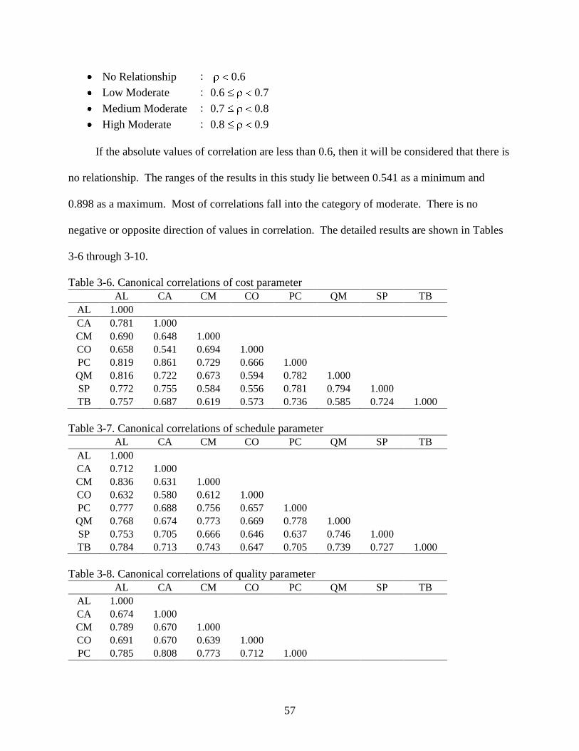
57
No Relationship : 0.6
Low Moderate : 0.6 0.7
Medium Moderate : 0.7 0.8
High Moderate : 0.8 0.9
If the absolute values of correlation are less than 0.6, then it will be considered that there is
no relationship. The ranges of the results in this study lie between 0.541 as a minimum and
0.898 as a maximum. Most of correlations fall into the category of moderate. There is no
negative or opposite direction of values in correlation. The detailed results are shown in Tables
3-6 through 3-10.
Table 3-6. Canonical correlations of cost parameter
AL CA CM CO PC QM SP TB
AL 1.000
CA 0.781 1.000
CM 0.690 0.648 1.000
CO 0.658 0.541 0.694 1.000
PC 0.819 0.861 0.729 0.666 1.000
QM 0.816 0.722 0.673 0.594 0.782 1.000
SP 0.772 0.755 0.584 0.556 0.781 0.794 1.000
TB 0.757 0.687 0.619 0.573 0.736 0.585 0.724 1.000
Table 3-7. Canonical correlations of schedule parameter
AL CA CM CO PC QM SP TB
AL 1.000
CA 0.712 1.000
CM 0.836 0.631 1.000
CO 0.632 0.580 0.612 1.000
PC 0.777 0.688 0.756 0.657 1.000
QM 0.768 0.674 0.773 0.669 0.778 1.000
SP 0.753 0.705 0.666 0.646 0.637 0.746 1.000
TB 0.784 0.713 0.743 0.647 0.705 0.739 0.727 1.000
Table 3-8. Canonical correlations of quality parameter
AL CA CM CO PC QM SP TB
AL 1.000
CA 0.674 1.000
CM 0.789 0.670 1.000
CO 0.691 0.670 0.639 1.000
PC 0.785 0.808 0.773 0.712 1.000
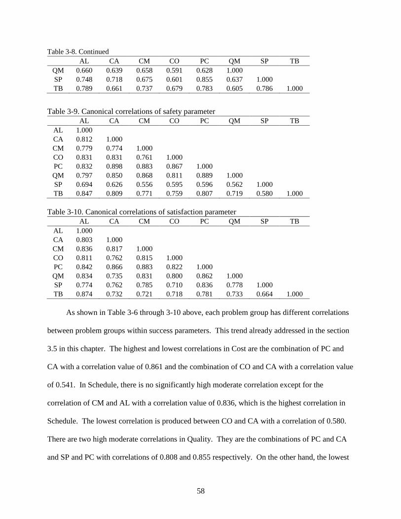
58
Table 3-8. Continued
AL CA CM CO PC QM SP TB
QM 0.660 0.639 0.658 0.591 0.628 1.000
SP 0.748 0.718 0.675 0.601 0.855 0.637 1.000
TB 0.789 0.661 0.737 0.679 0.783 0.605 0.786 1.000
Table 3-9. Canonical correlations of safety parameter
AL CA CM CO PC QM SP TB
AL 1.000
CA 0.812 1.000
CM 0.779 0.774 1.000
CO 0.831 0.831 0.761 1.000
PC 0.832 0.898 0.883 0.867 1.000
QM 0.797 0.850 0.868 0.811 0.889 1.000
SP 0.694 0.626 0.556 0.595 0.596 0.562 1.000
TB 0.847 0.809 0.771 0.759 0.807 0.719 0.580 1.000
Table 3-10. Canonical correlations of satisfaction parameter
AL CA CM CO PC QM SP TB
AL 1.000
CA 0.803 1.000
CM 0.836 0.817 1.000
CO 0.811 0.762 0.815 1.000
PC 0.842 0.866 0.883 0.822 1.000
QM 0.834 0.735 0.831 0.800 0.862 1.000
SP 0.774 0.762 0.785 0.710 0.836 0.778 1.000
TB 0.874 0.732 0.721 0.718 0.781 0.733 0.664 1.000
As shown in Table 3-6 through 3-10 above, each problem group has different correlations
between problem groups within success parameters. This trend already addressed in the section
3.5 in this chapter. The highest and lowest correlations in Cost are the combination of PC and
CA with a correlation value of 0.861 and the combination of CO and CA with a correlation value
of 0.541. In Schedule, there is no significantly high moderate correlation except for the
correlation of CM and AL with a correlation value of 0.836, which is the highest correlation in
Schedule. The lowest correlation is produced between CO and CA with a correlation of 0.580.
There are two high moderate correlations in Quality. They are the combinations of PC and CA
and SP and PC with correlations of 0.808 and 0.855 respectively. On the other hand, the lowest
59
correlation is 0.591 of the combination of QM and CO. The highest correlation in Safety is
0.898, which is the combination of PC and CA. The lowest correlation in Safety is 0.556 from
the combination of SP and CM. There are more correlations of less than or equal to 0.6 in Safety,
especially the most of combinations with SP, compared to other success parameters. The highest
correlation is the combination of PC and CM with a correlation of 0.883 and the lowest
correlation is 0.664 by the combination of TB and SP in Satisfaction. There is no correlation less
than or equal to 0.6 in this parameter. In Safety and Satisfaction parameters, the most of problem
groups show medium and high moderate correlations. The number of high moderate correlations
is larger than that of Cost, Schedule, and Quality parameter. It clearly shows that a few
combinations of problem groups have high correlations in Cost, Schedule, and Quality
parameters. In other words, some problem groups have some tendencies for high correlations in
those success parameters. But most of combinations in Safety and Satisfaction parameters
usually have high correlations. It depicts that most of problems in these parameters have
tendencies for high correlations, compared to another three parameters.
Factor Analysis (Exploratory vs. Confirmatory)
One of the main purposes of this research is to define the relationships between problem
groups and success parameters. To achieve this goal, the proper methodology has to be chosen,
considering the data available. The data available are the negative impacts of problems on each
success parameter. To satisfy the data set and purpose of this research, confirmatory factor
analysis (CFA) has been chosen. Before CFA is addressed, the general concepts of factor
analysis will be discussed.
Factor analysis is commonly used in education, sociology, and psychology because it is
sometimes impossible to measure directly the variables effects in these disciplines. Factor
analysis is a statistical procedure for uncovering factors by observed variables. The main
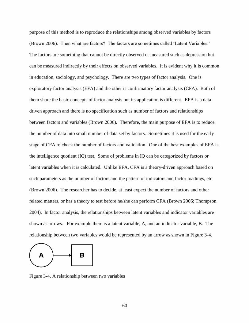
60
purpose of this method is to reproduce the relationships among observed variables by factors
(Brown 2006). Then what are factors? The factors are sometimes called „Latent Variables.‟
The factors are something that cannot be directly observed or measured such as depression but
can be measured indirectly by their effects on observed variables. It is evident why it is common
in education, sociology, and psychology. There are two types of factor analysis. One is
exploratory factor analysis (EFA) and the other is confirmatory factor analysis (CFA). Both of
them share the basic concepts of factor analysis but its application is different. EFA is a data-
driven approach and there is no specification such as number of factors and relationships
between factors and variables (Brown 2006). Therefore, the main purpose of EFA is to reduce
the number of data into small number of data set by factors. Sometimes it is used for the early
stage of CFA to check the number of factors and validation. One of the best examples of EFA is
the intelligence quotient (IQ) test. Some of problems in IQ can be categorized by factors or
latent variables when it is calculated. Unlike EFA, CFA is a theory-driven approach based on
such parameters as the number of factors and the pattern of indicators and factor loadings, etc
(Brown 2006). The researcher has to decide, at least expect the number of factors and other
related matters, or has a theory to test before he/she can perform CFA (Brown 2006; Thompson
2004). In factor analysis, the relationships between latent variables and indicator variables are
shown as arrows. For example there is a latent variable, A, and an indicator variable, B. The
relationship between two variables would be represented by an arrow as shown in Figure 3-4.
A BA B
Figure 3-4. A relationship between two variables
61
A relationship depicted by an arrow in factor analysis is considered as a causal relationship
(Brown 2006). In Figure 3-4, the relationship between A and B is a causal relationship. It
means that the latent variable, A, causes the indicator variable, B. In another words, the variable,
A, could be explained by the variable, B. “The main concern of CFA is to evaluate how well a
CFA model (S) reproduces the sample covariance matrix (S) of the measured variables” (Brown
2006). The researcher has to find the best-fitted model explained by the sample covariance
matrix. In this section, the overall concepts of factor analysis have been discussed. Although the
main methodology of this research is CFA, it is necessary to address the concept of EFA in detail
because both of them share the same methodology and terminologies.
Exploratory Factor Analysis (EFA)
Overview
The overall concepts of factor analysis in EFA and CFA have been discussed above.
Before CFA is discussed in detail, it is helpful to discuss EFA first to understand CFA. All the
terminologies and components are common to both EFA and CFA. In this section, the main
concepts and purposes of EFA will be shown with some examples.
The concepts of factor or latent variables have already been addressed previously. The
main purposes of factor analysis can be summarized as shown below (Thompson 2004):
1) Evaluation of score validation
2) Development of theory regarding nature of construct
3) Summary of relationships using factor
These three purposes do not always fall into the category of EFA. The last two are
commonly used for EFA. The most common purpose of EFA would possibly be „Summary of
relationships using factor‟. In another words, it is possible to explore the potential relationships
or look for a pattern, trend, or characteristics using EFA in a set of data. Based on this
exploration, the researcher could develop and test a theory using CFA. During an EFA process,
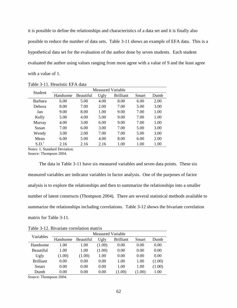
62
it is possible to define the relationships and characteristics of a data set and it is finally also
possible to reduce the number of data sets. Table 3-11 shows an example of EFA data. This is a
hypothetical data set for the evaluation of the author done by seven students. Each student
evaluated the author using values ranging from most agree with a value of 9 and the least agree
with a value of 1.
Table 3-11. Heuristic EFA data
Student Measured Variable
Handsome Beautiful Ugly Brilliant Smart Dumb
Barbara 6.00 5.00 4.00 8.00 6.00 2.00
Debora 8.00 7.00 2.00 7.00 5.00 3.00
Jan 9.00 8.00 1.00 9.00 7.00 1.00
Kelly 5.00 4.00 5.00 9.00 7.00 1.00
Murray 4.00 3.00 6.00 9.00 7.00 1.00
Susan 7.00 6.00 3.00 7.00 5.00 3.00
Wendy 3.00 2.00 7.00 7.00 5.00 3.00
Mean 6.00 5.00 4.00 8.00 6.00 2.00
S.D.1 2.16 2.16 2.16 1.00 1.00 1.00
Notes: 1. Standard Deviation.
Source: Thompson 2004.
The data in Table 3-11 have six measured variables and seven data points. These six
measured variables are indicator variables in factor analysis. One of the purposes of factor
analysis is to explore the relationships and then to summarize the relationships into a smaller
number of latent constructs (Thompson 2004). There are several statistical methods available to
summarize the relationships including correlations. Table 3-12 shows the bivariate correlation
matrix for Table 3-11.
Table 3-12. Bivariate correlation matrix
Variables Measured Variable
Handsome Beautiful Ugly Brilliant Smart Dumb
Handsome 1.00 1.00 (1.00) 0.00 0.00 0.00
Beautiful 1.00 1.00 (1.00) 0.00 0.00 0.00
Ugly (1.00) (1.00) 1.00 0.00 0.00 0.00
Brilliant 0.00 0.00 0.00 1.00 1.00 (1.00)
Smart 0.00 0.00 0.00 1.00 1.00 (1.00)
Dumb 0.00 0.00 0.00 (1.00) (1.00) 1.00
Source: Thompson 2004.
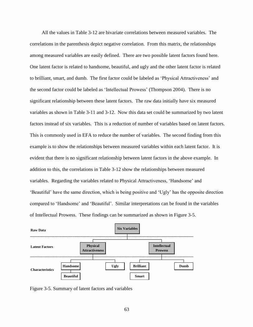
63
All the values in Table 3-12 are bivariate correlations between measured variables. The
correlations in the parenthesis depict negative correlation. From this matrix, the relationships
among measured variables are easily defined. There are two possible latent factors found here.
One latent factor is related to handsome, beautiful, and ugly and the other latent factor is related
to brilliant, smart, and dumb. The first factor could be labeled as „Physical Attractiveness‟ and
the second factor could be labeled as „Intellectual Prowess‟ (Thompson 2004). There is no
significant relationship between these latent factors. The raw data initially have six measured
variables as shown in Table 3-11 and 3-12. Now this data set could be summarized by two latent
factors instead of six variables. This is a reduction of number of variables based on latent factors.
This is commonly used in EFA to reduce the number of variables. The second finding from this
example is to show the relationships between measured variables within each latent factor. It is
evident that there is no significant relationship between latent factors in the above example. In
addition to this, the correlations in Table 3-12 show the relationships between measured
variables. Regarding the variables related to Physical Attractiveness, „Handsome‟ and
„Beautiful‟ have the same direction, which is being positive and „Ugly‟ has the opposite direction
compared to „Handsome‟ and „Beautiful‟. Similar interpretations can be found in the variables
of Intellectual Prowess. These findings can be summarized as shown in Figure 3-5.
Latent Factors
Characteristics
Raw Data
Beautiful
Brilliant
Smart
Dumb
Six Variables
Physical
Attractiveness
Intellectual
Prowess
Handsome Ugly
Figure 3-5. Summary of latent factors and variables
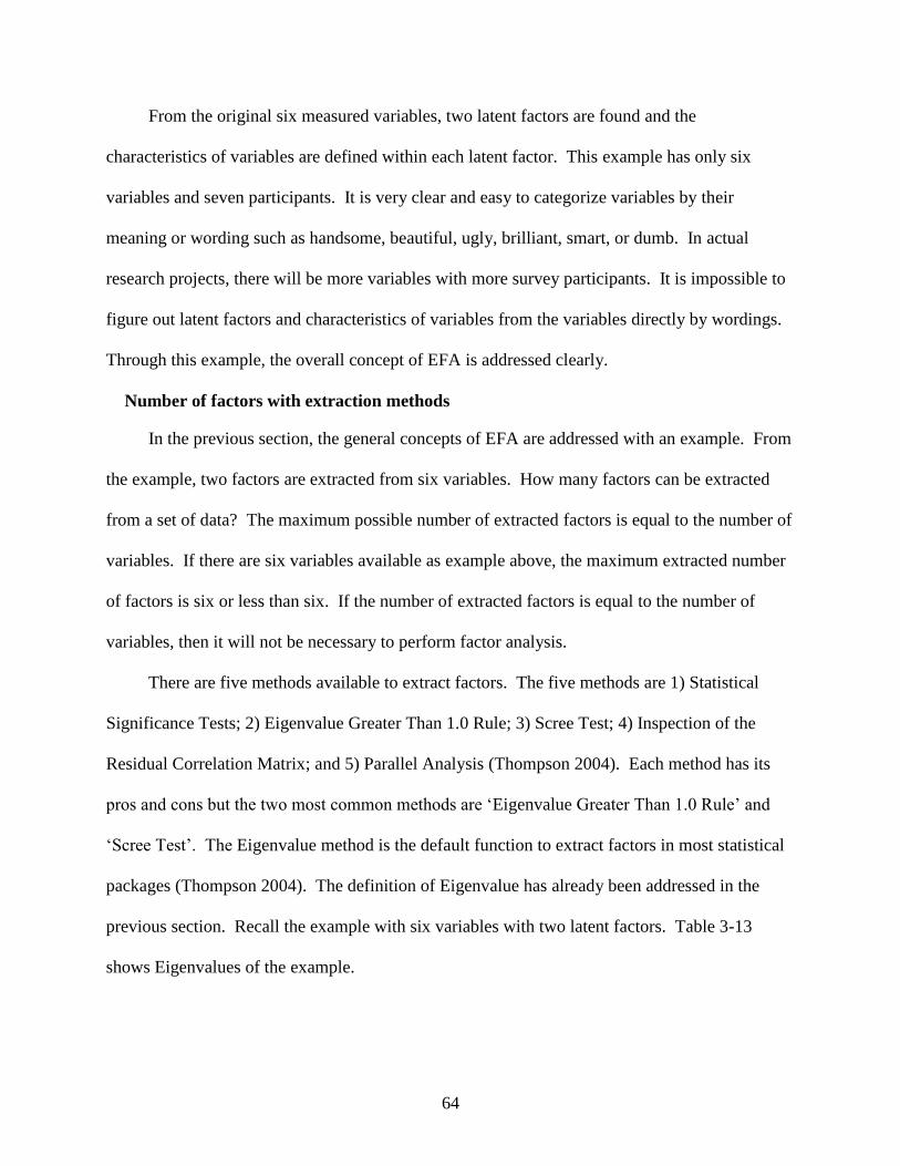
64
From the original six measured variables, two latent factors are found and the
characteristics of variables are defined within each latent factor. This example has only six
variables and seven participants. It is very clear and easy to categorize variables by their
meaning or wording such as handsome, beautiful, ugly, brilliant, smart, or dumb. In actual
research projects, there will be more variables with more survey participants. It is impossible to
figure out latent factors and characteristics of variables from the variables directly by wordings.
Through this example, the overall concept of EFA is addressed clearly.
Number of factors with extraction methods
In the previous section, the general concepts of EFA are addressed with an example. From
the example, two factors are extracted from six variables. How many factors can be extracted
from a set of data? The maximum possible number of extracted factors is equal to the number of
variables. If there are six variables available as example above, the maximum extracted number
of factors is six or less than six. If the number of extracted factors is equal to the number of
variables, then it will not be necessary to perform factor analysis.
There are five methods available to extract factors. The five methods are 1) Statistical
Significance Tests; 2) Eigenvalue Greater Than 1.0 Rule; 3) Scree Test; 4) Inspection of the
Residual Correlation Matrix; and 5) Parallel Analysis (Thompson 2004). Each method has its
pros and cons but the two most common methods are „Eigenvalue Greater Than 1.0 Rule‟ and
„Scree Test‟. The Eigenvalue method is the default function to extract factors in most statistical
packages (Thompson 2004). The definition of Eigenvalue has already been addressed in the
previous section. Recall the example with six variables with two latent factors. Table 3-13
shows Eigenvalues of the example.
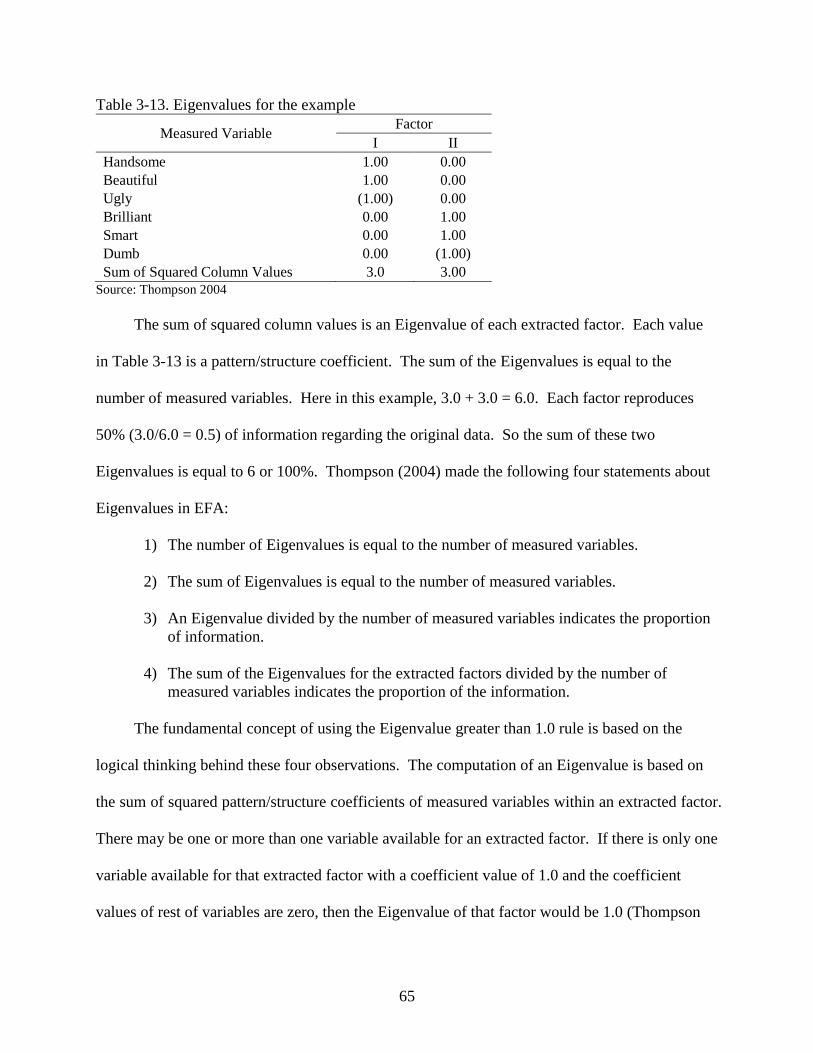
65
Table 3-13. Eigenvalues for the example
Measured Variable Factor
I II
Handsome 1.00 0.00
Beautiful 1.00 0.00
Ugly (1.00) 0.00
Brilliant 0.00 1.00
Smart 0.00 1.00
Dumb 0.00 (1.00)
Sum of Squared Column Values 3.0 3.00
Source: Thompson 2004
The sum of squared column values is an Eigenvalue of each extracted factor. Each value
in Table 3-13 is a pattern/structure coefficient. The sum of the Eigenvalues is equal to the
number of measured variables. Here in this example, 3.0 + 3.0 = 6.0. Each factor reproduces
50% (3.0/6.0 = 0.5) of information regarding the original data. So the sum of these two
Eigenvalues is equal to 6 or 100%. Thompson (2004) made the following four statements about
Eigenvalues in EFA:
1) The number of Eigenvalues is equal to the number of measured variables.
2) The sum of Eigenvalues is equal to the number of measured variables.
3) An Eigenvalue divided by the number of measured variables indicates the proportion
of information.
4) The sum of the Eigenvalues for the extracted factors divided by the number of
measured variables indicates the proportion of the information.
The fundamental concept of using the Eigenvalue greater than 1.0 rule is based on the
logical thinking behind these four observations. The computation of an Eigenvalue is based on
the sum of squared pattern/structure coefficients of measured variables within an extracted factor.
There may be one or more than one variable available for an extracted factor. If there is only one
variable available for that extracted factor with a coefficient value of 1.0 and the coefficient
values of rest of variables are zero, then the Eigenvalue of that factor would be 1.0 (Thompson
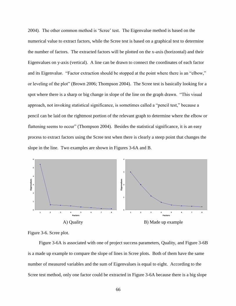
66
2004). The other common method is „Scree‟ test. The Eigenvalue method is based on the
numerical value to extract factors, while the Scree test is based on a graphical test to determine
the number of factors. The extracted factors will be plotted on the x-axis (horizontal) and their
Eigenvalues on y-axis (vertical). A line can be drawn to connect the coordinates of each factor
and its Eigenvalue. “Factor extraction should be stopped at the point where there is an “elbow,”
or leveling of the plot” (Brown 2006; Thompson 2004). The Scree test is basically looking for a
spot where there is a sharp or big change in slope of the line on the graph drawn. “This visual
approach, not invoking statistical significance, is sometimes called a “pencil test,” because a
pencil can be laid on the rightmost portion of the relevant graph to determine where the elbow or
flattening seems to occur” (Thompson 2004). Besides the statistical significance, it is an easy
process to extract factors using the Scree test when there is clearly a steep point that changes the
slope in the line. Two examples are shown in Figures 3-6A and B.
0
1
2
3
4
5
6
1 2 3 4 5 6 7 8
Factors
Eig
en
va
lue
s
0
1
2
3
4
1 2 3 4 5 6 7 8
Factors
Eig
en
va
lue
s
A) Quality B) Made up example
Figure 3-6. Scree plot.
Figure 3-6A is associated with one of project success parameters, Quality, and Figure 3-6B
is a made up example to compare the slope of lines in Scree plots. Both of them have the same
number of measured variables and the sum of Eigenvalues is equal to eight. According to the
Scree test method, only one factor could be extracted in Figure 3-6A because there is a big slope
67
change at „Factor 2‟ in the plot. From that point, there are no big slope changes until the last
potential factor, „Factor 8‟. On the other hand Figure 3-6B has no significant changes in slope.
In this case, it would be impossible to extract factors using the Scree test method.
The Eigenvalue greater than 1.0 and the Scree test are two most common methods to
extract factors. These two methods are available on most statistical computer packages such as
the Statistical Analysis Software (SAS ) and the Statistical Package for the Social Sciences
(SPSS ). EFA will be performed as the preliminary stage of CFA even though the main
methodology of this research is CFA. The method to be used to extract factors would be the
combined Eigenvalue method and Scree test.
Confirmatory Factor Analysis (CFA)
Overview
The overall concepts of factor analysis for EFA and CFA have been addressed and the
background of EFA has been discussed in more detail so far. The reason why CFA has been
chosen for this research has been explained as well. In this section, the parameters of factor
analysis models and an example relating to CFA factor analysis will be discussed.
There are five terms in general factor analysis models. They are factor loadings ( ), factor
variances (2), unique variances ( ), exogenous (independent) variables, and endogenous
(dependent) variables. The explanation of these are as follows (Brown 2006):
Factor Loadings ( ): Normally factor loadings are regression slopes between latent
variables and indicator variables. Sometimes they can be correlations when there is no
cross loading between latent variables and indicator variables.
Factor Variances (2): Factor variances are variances explained by latent factors.
Unique Variances ( = 1 - 2): Unique variances are variances that are not explained by
latent factors. This is the difference between factor analysis and multiple regressions.
Factor analysis considers the measurement error.
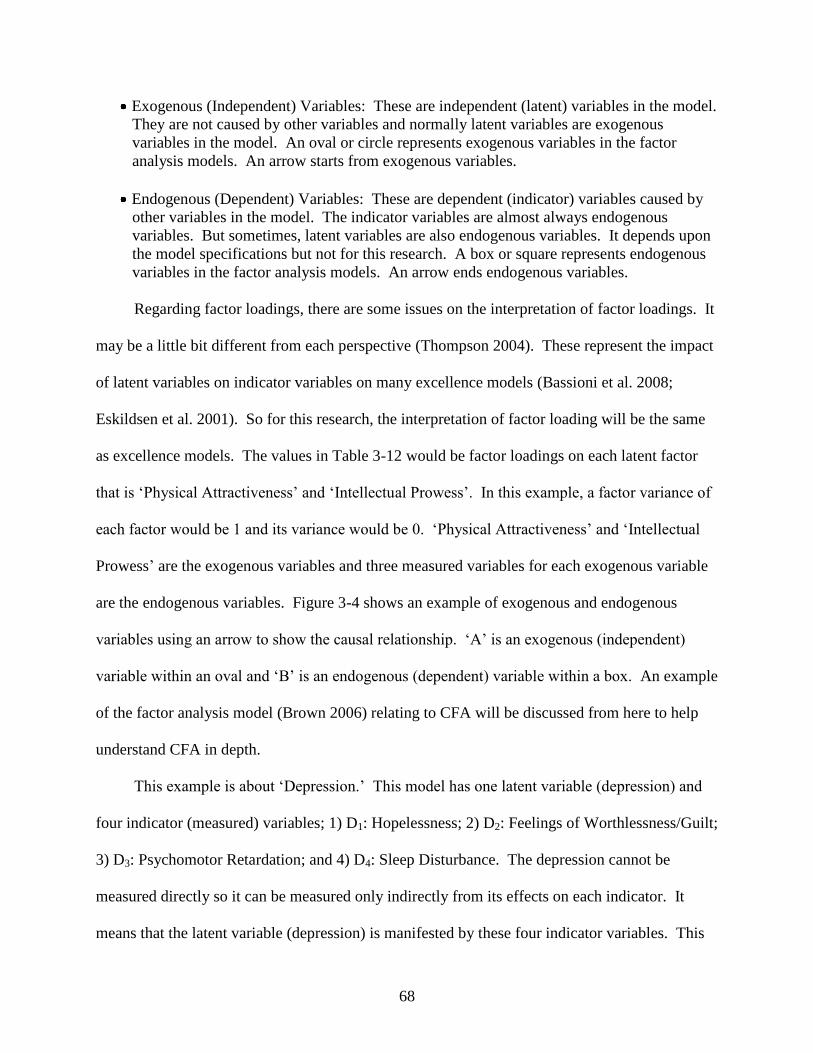
68
Exogenous (Independent) Variables: These are independent (latent) variables in the model.
They are not caused by other variables and normally latent variables are exogenous
variables in the model. An oval or circle represents exogenous variables in the factor
analysis models. An arrow starts from exogenous variables.
Endogenous (Dependent) Variables: These are dependent (indicator) variables caused by
other variables in the model. The indicator variables are almost always endogenous
variables. But sometimes, latent variables are also endogenous variables. It depends upon
the model specifications but not for this research. A box or square represents endogenous
variables in the factor analysis models. An arrow ends endogenous variables.
Regarding factor loadings, there are some issues on the interpretation of factor loadings. It
may be a little bit different from each perspective (Thompson 2004). These represent the impact
of latent variables on indicator variables on many excellence models (Bassioni et al. 2008;
Eskildsen et al. 2001). So for this research, the interpretation of factor loading will be the same
as excellence models. The values in Table 3-12 would be factor loadings on each latent factor
that is „Physical Attractiveness‟ and „Intellectual Prowess‟. In this example, a factor variance of
each factor would be 1 and its variance would be 0. „Physical Attractiveness‟ and „Intellectual
Prowess‟ are the exogenous variables and three measured variables for each exogenous variable
are the endogenous variables. Figure 3-4 shows an example of exogenous and endogenous
variables using an arrow to show the causal relationship. „A‟ is an exogenous (independent)
variable within an oval and „B‟ is an endogenous (dependent) variable within a box. An example
of the factor analysis model (Brown 2006) relating to CFA will be discussed from here to help
understand CFA in depth.
This example is about „Depression.‟ This model has one latent variable (depression) and
four indicator (measured) variables; 1) D1: Hopelessness; 2) D2: Feelings of Worthlessness/Guilt;
3) D3: Psychomotor Retardation; and 4) D4: Sleep Disturbance. The depression cannot be
measured directly so it can be measured only indirectly from its effects on each indicator. It
means that the latent variable (depression) is manifested by these four indicator variables. This
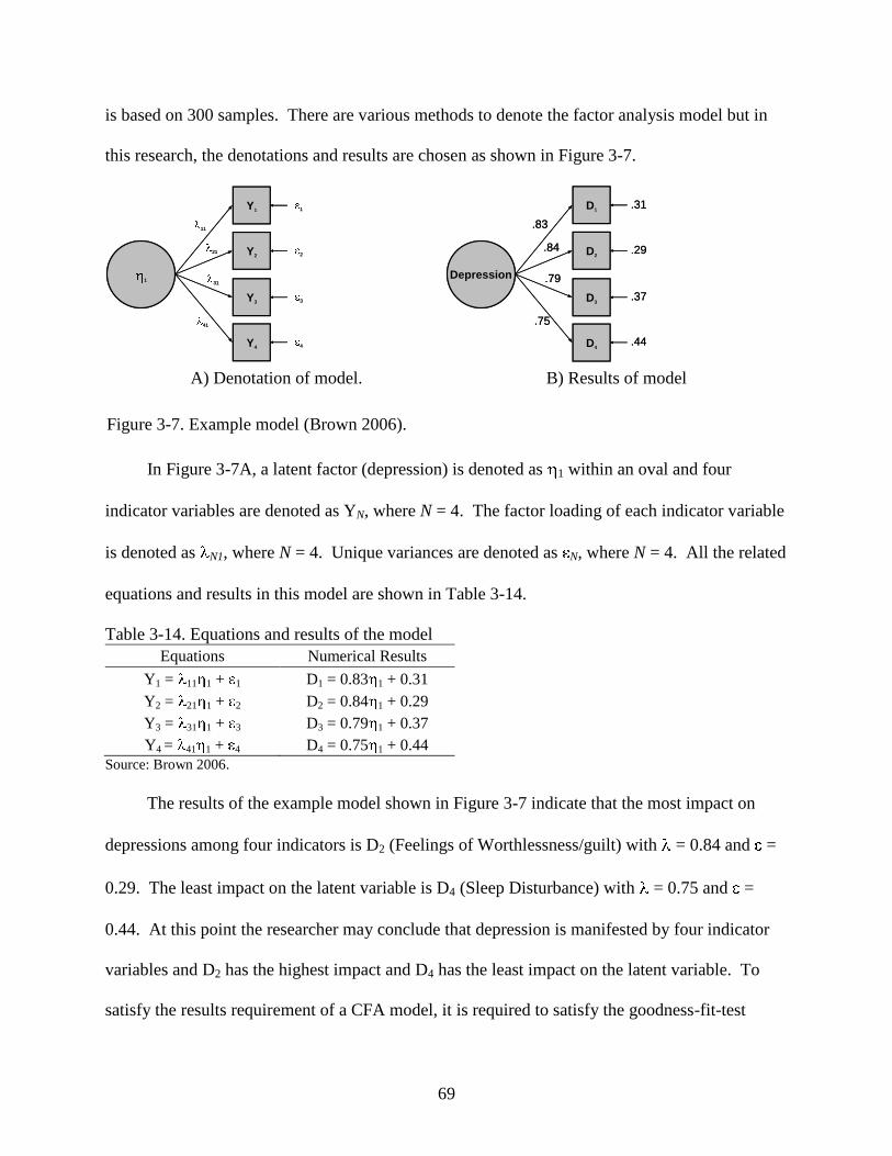
69
is based on 300 samples. There are various methods to denote the factor analysis model but in
this research, the denotations and results are chosen as shown in Figure 3-7.
1
2
4
3
Y4
1
Y3
Y2
Y1
11
21
31
41
1
2
4
3
Y4
1
Y3
Y2
Y1
11
21
31
41
.31
.29
.44
.37
D4
Depression
D3
D2
D1
.83
.84
.79
.75
.31
.29
.44
.37
D4
Depression
D3
D2
D1
.83
.84
.79
.75
A) Denotation of model. B) Results of model
Figure 3-7. Example model (Brown 2006).
In Figure 3-7A, a latent factor (depression) is denoted as 1 within an oval and four
indicator variables are denoted as YN, where N = 4. The factor loading of each indicator variable
is denoted as N1, where N = 4. Unique variances are denoted as N, where N = 4. All the related
equations and results in this model are shown in Table 3-14.
Table 3-14. Equations and results of the model
Equations Numerical Results
Y1 = 11 1 + 1 D1 = 0.83 1 + 0.31
Y2 = 21 1 + 2 D2 = 0.84 1 + 0.29
Y3 = 31 1 + 3 D3 = 0.79 1 + 0.37
Y4 = 41 1 + 4 D4 = 0.75 1 + 0.44
Source: Brown 2006.
The results of the example model shown in Figure 3-7 indicate that the most impact on
depressions among four indicators is D2 (Feelings of Worthlessness/guilt) with = 0.84 and =
0.29. The least impact on the latent variable is D4 (Sleep Disturbance) with = 0.75 and =
0.44. At this point the researcher may conclude that depression is manifested by four indicator
variables and D2 has the highest impact and D4 has the least impact on the latent variable. To
satisfy the results requirement of a CFA model, it is required to satisfy the goodness-fit-test
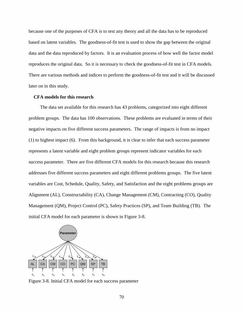
70
because one of the purposes of CFA is to test any theory and all the data has to be reproduced
based on latent variables. The goodness-of-fit test is used to show the gap between the original
data and the data reproduced by factors. It is an evaluation process of how well the factor model
reproduces the original data. So it is necessary to check the goodness-of-fit test in CFA models.
There are various methods and indices to perform the goodness-of-fit test and it will be discussed
later on in this study.
CFA models for this research
The data set available for this research has 43 problems, categorized into eight different
problem groups. The data has 100 observations. These problems are evaluated in terms of their
negative impacts on five different success parameters. The range of impacts is from no impact
(1) to highest impact (6). From this background, it is clear to infer that each success parameter
represents a latent variable and eight problem groups represent indicator variables for each
success parameter. There are five different CFA models for this research because this research
addresses five different success parameters and eight different problems groups. The five latent
variables are Cost, Schedule, Quality, Safety, and Satisfaction and the eight problems groups are
Alignment (AL), Constructability (CA), Change Management (CM), Contracting (CO), Quality
Management (QM), Project Control (PC), Safety Practices (SP), and Team Building (TB). The
initial CFA model for each parameter is shown in Figure 3-8.
Parameter
431 2
AL CA CM CO
1P 2P 3P 4P
875 6
PC QM SP TB
8P5P 6P 7P
Parameter
431 2
AL CA CM CO
1P 2P 3P 4P
875 6
PC QM SP TB
8P5P 6P 7P
Figure 3-8. Initial CFA model for each success parameter
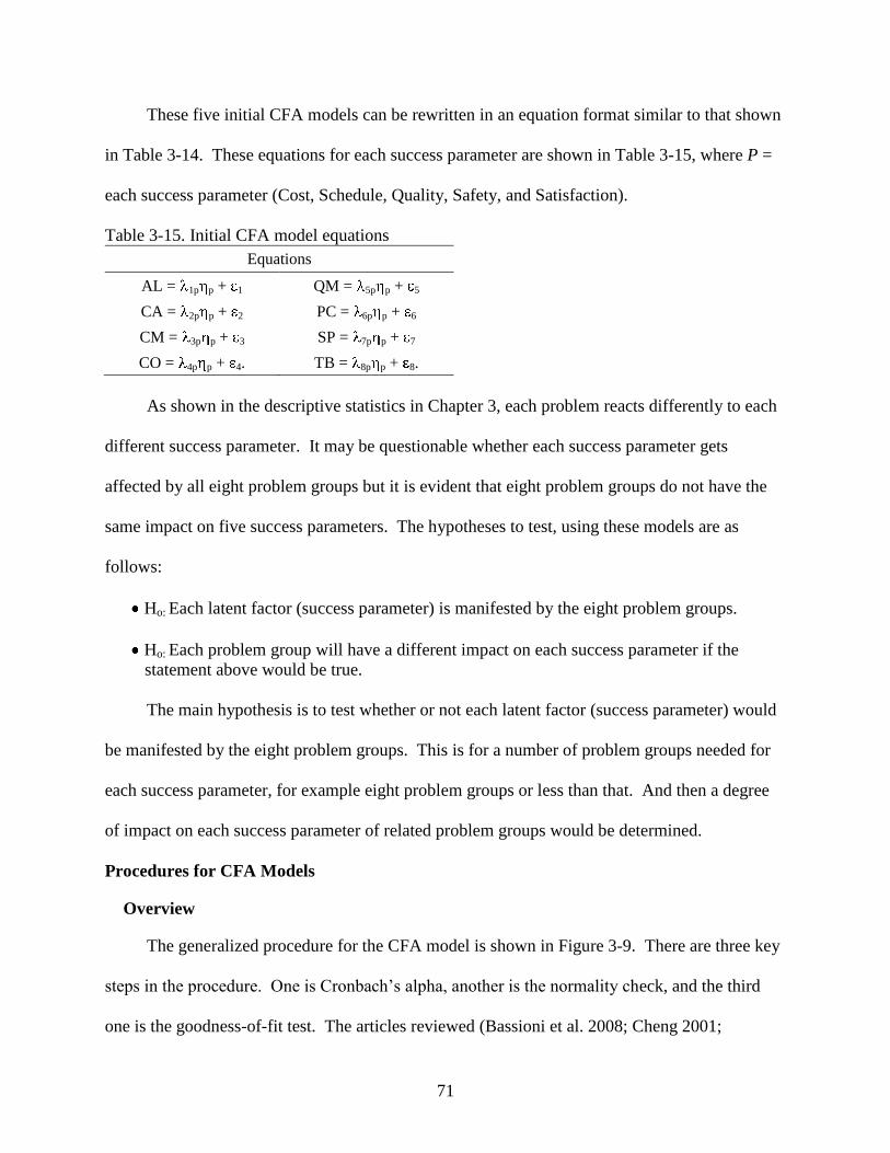
71
These five initial CFA models can be rewritten in an equation format similar to that shown
in Table 3-14. These equations for each success parameter are shown in Table 3-15, where P =
each success parameter (Cost, Schedule, Quality, Safety, and Satisfaction).
Table 3-15. Initial CFA model equations
Equations
AL = 1p p + 1 QM = 5p p + 5
CA = 2p p + 2 PC = 6p p + 6
CM = 3p p + 3 SP = 7p p + 7
CO = 4p p + 4. TB = 8p p + 8.
As shown in the descriptive statistics in Chapter 3, each problem reacts differently to each
different success parameter. It may be questionable whether each success parameter gets
affected by all eight problem groups but it is evident that eight problem groups do not have the
same impact on five success parameters. The hypotheses to test, using these models are as
follows:
Ho: Each latent factor (success parameter) is manifested by the eight problem groups.
Ho: Each problem group will have a different impact on each success parameter if the
statement above would be true.
The main hypothesis is to test whether or not each latent factor (success parameter) would
be manifested by the eight problem groups. This is for a number of problem groups needed for
each success parameter, for example eight problem groups or less than that. And then a degree
of impact on each success parameter of related problem groups would be determined.
Procedures for CFA Models
Overview
The generalized procedure for the CFA model is shown in Figure 3-9. There are three key
steps in the procedure. One is Cronbach‟s alpha, another is the normality check, and the third
one is the goodness-of-fit test. The articles reviewed (Bassioni et al. 2008; Cheng 2001;
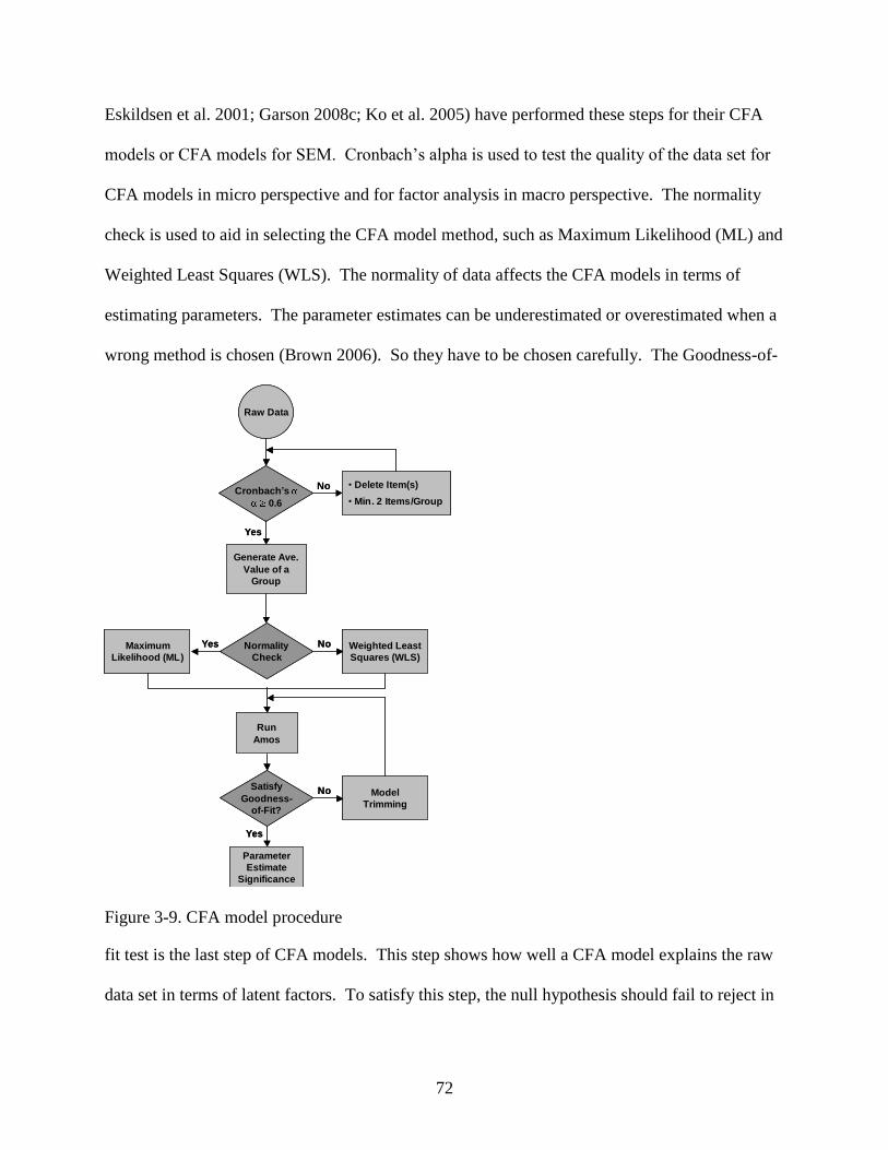
72
Eskildsen et al. 2001; Garson 2008c; Ko et al. 2005) have performed these steps for their CFA
models or CFA models for SEM. Cronbach‟s alpha is used to test the quality of the data set for
CFA models in micro perspective and for factor analysis in macro perspective. The normality
check is used to aid in selecting the CFA model method, such as Maximum Likelihood (ML) and
Weighted Least Squares (WLS). The normality of data affects the CFA models in terms of
estimating parameters. The parameter estimates can be underestimated or overestimated when a
wrong method is chosen (Brown 2006). So they have to be chosen carefully. The Goodness-of-
Raw Data
Cronbach’s
0.6
• Delete Item(s)
• Min. 2 Items/Group
Generate Ave.
Value of a
Group
Yes
No
Normality
Check
Weighted Least
Squares (WLS)
Run
Amos
Yes
NoMaximum
Likelihood (ML)
Yes
Satisfy
Goodness-
of-Fit?
Model
Trimming
Parameter
Estimate
Significance
No
Raw Data
Cronbach’s
0.6
• Delete Item(s)
• Min. 2 Items/Group
Generate Ave.
Value of a
Group
Yes
No
Normality
Check
Weighted Least
Squares (WLS)
Run
Amos
Yes
NoMaximum
Likelihood (ML)
Yes
Satisfy
Goodness-
of-Fit?
Model
Trimming
Parameter
Estimate
Significance
No
Figure 3-9. CFA model procedure
fit test is the last step of CFA models. This step shows how well a CFA model explains the raw
data set in terms of latent factors. To satisfy this step, the null hypothesis should fail to reject in
73
the case of 2 for example a p value has to be greater than 0.05 at α = 0.05. There are various
methods for the goodness-of-fit tests and they will be discussed later.
There is a difference between all the articles reviewed and the procedure in Figure 3-9.
Only one article addresses the improvement of CFA model goodness-of-fit test by deleting some
of paths in the model (Garson 2008c). The rest of articles do not address the model trimming.
The reasons why they do not explain this step may be:
The CFA model satisfies the goodness-of-fit test.
The CFA model does not satisfy the goodness-of-fit test but the goodness-of-fit test result
falls into a certain excusable range from the researcher‟s perspective (There are no specific
or official guidelines for this).
One of the purposes of CFA models is to test a theory. If the null hypothesis gets rejected
and/or the goodness-of-fit test does not meet, then the theory is not right regarding at least
what it says. So it is not necessary to improve CFA models in this case because it is proven
to be wrong.
If the goodness-of-test does not meet the required criteria, then there is a difference
between a model and a set of data and it could mean that the theory to be tested is wrong. As
mentioned earlier, if any CFA models do not meet the goodness-of-fit test, then the CFA models
will be trimmed until the goodness-of-fit test is satisfied. All eight problem groups may not
result in major impacts on each success parameter even though each problem group may have
different impacts. The model trimming procedure will be necessary to find those problem
groups that may not manifest in impacts on each success parameter. More detailed information
on each step will be discussed in the following sections.
Crobach’s (Coefficient) alpha
The first step is to check Cronbach‟s alpha ( ), which is also called „Coefficient Alpha‟ or
„Reliability Coefficient‟ (Garson 2008b). The Cronbach‟s alpha is a measure of the internal
consistency of a scale and the higher the alpha value is the better (Garson 2008c; Spector 1992).
74
“Alpha measures the extent to which item responses obtained at the same time correlate highly
with each other” (Garson 2008b). The alpha value represents a direct function of both the
number of items and their magnitude of intercorrelation. The range of alpha is from 0 to 1
(Garson 2008c). The number of items and intercorrelation affect the alpha value. Cronbach‟s
alpha normally has higher values when there is a higher number of items. The main use of
Cronbach‟s alpha is to check that everything is measured that has to be measured in the same
way. The checking process is sometimes referred to as checking “Construct” (Garson 2008b). It
is assumed that there is an error if an item is less correlated with others (Spector 1992). For
example, if everybody measures something in common, then the measurements will be highly
correlated with each other. The computation of alpha value is shown in Equation 3-3 (Spector
1992).
= k
T
2 - I
2
(Equation 3-3) k - 1 T
2
Where,
k : Number of items
T2 : Total variance of the sum of the items
I2 : Total variance of an individual item
To use the raw data for CFA models, the coefficient alpha values have to be checked. The
acceptable range of coefficient alpha values varies by authors, with requiring a value greater than
0.6 (Bassioni et al. 2008; Hair et al. 1998) or 0.7 (Garson 2008b; Garson 2008c) even though all
agree that the higher the value is the better. For this research, the minimum acceptable
Cronbach‟s alpha value is greater than 0.6. If some Cronbach‟s alpha value is less than 0.6, then
it will be retained and not deleted because there are only eight problem groups available here. In
other words, there are not too many variables available for CFA models. The Cronbach‟s alpha
values will be interpreted as the guidelines for each success parameter.
75
In each problem group of each success parameter, the coefficient alpha values will be
computed. If an initial alpha value is less than 0.6, then one or more items will be deleted until a
recomputed alpha value is greater than 0.6. The statistical computer program, SPSS , provides
the expected alpha value if an item is deleted. Even though the researcher could delete as many
items as he/she wants to satisfy the minimum coefficient values, at least, two items need to be
retained in each problem group (Bassioni et al. 2008). After this procedure, the number of items
in each problem group of each success parameter will be determined for the next step.
Average values of groups of each success parameter
There will be maximum 43 problems available for eight problem groups after the
computation of the coefficient alpha. There is a chance that some success parameters have less
than 43 problems. The number of items in each group will vary, depending on the Cronbach‟s
alpha values. So the same concept that is based on the problem groups not the individual
problems of canonical correlation is applied to this step. To get the value of each problem group,
the average value is computed and applied for each success parameter. After the computation of
the Cronbach‟s alpha, the original value of remaining items will be used for the computation of
the average value of each problem group in each success parameter. Eight average values for
each success parameter will be available for normality check.
Data normality
There are two major estimation methods in CFA models. They are the Maximum
Likelihood (ML) and the Weighted Least Squares (WLS) method. Both of them are popular in
CFA models. But the major difference in between these two methods is the data normality. To
use ML method, the data should be normal otherwise WLS has to be used for CFA models. As
mentioned earlier, there will be a underestimated or overestimated parameter if a wrong estimate
method is chosen for a set of data (Brown 2006). Regarding the data normality, there are two
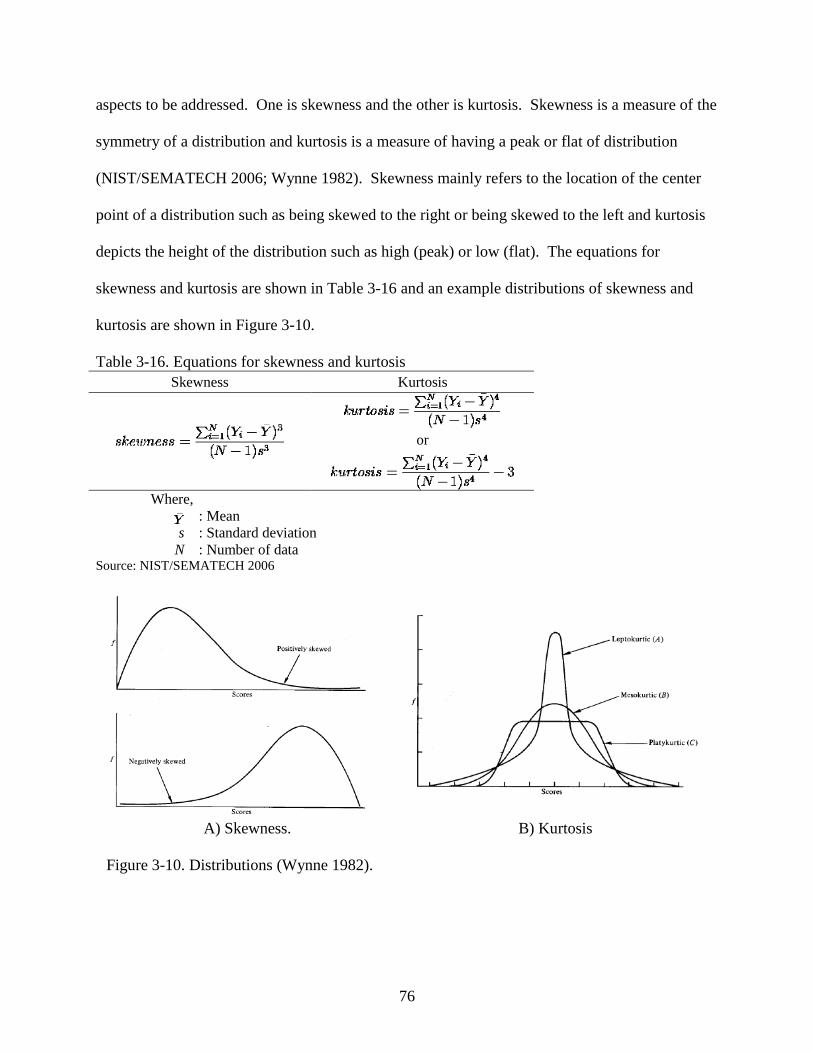
76
aspects to be addressed. One is skewness and the other is kurtosis. Skewness is a measure of the
symmetry of a distribution and kurtosis is a measure of having a peak or flat of distribution
(NIST/SEMATECH 2006; Wynne 1982). Skewness mainly refers to the location of the center
point of a distribution such as being skewed to the right or being skewed to the left and kurtosis
depicts the height of the distribution such as high (peak) or low (flat). The equations for
skewness and kurtosis are shown in Table 3-16 and an example distributions of skewness and
kurtosis are shown in Figure 3-10.
Table 3-16. Equations for skewness and kurtosis
Skewness Kurtosis
or
Where,
: Mean
s : Standard deviation
N : Number of data Source: NIST/SEMATECH 2006
A) Skewness. B) Kurtosis
Figure 3-10. Distributions (Wynne 1982).
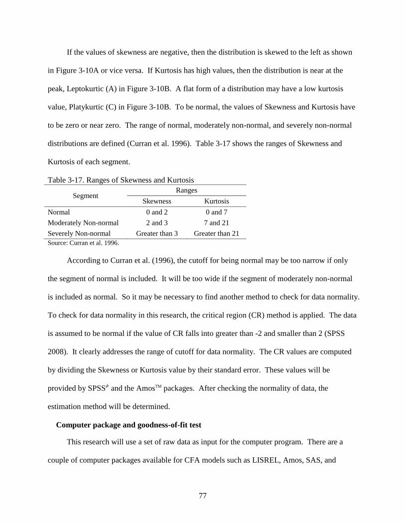
77
If the values of skewness are negative, then the distribution is skewed to the left as shown
in Figure 3-10A or vice versa. If Kurtosis has high values, then the distribution is near at the
peak, Leptokurtic (A) in Figure 3-10B. A flat form of a distribution may have a low kurtosis
value, Platykurtic (C) in Figure 3-10B. To be normal, the values of Skewness and Kurtosis have
to be zero or near zero. The range of normal, moderately non-normal, and severely non-normal
distributions are defined (Curran et al. 1996). Table 3-17 shows the ranges of Skewness and
Kurtosis of each segment.
Table 3-17. Ranges of Skewness and Kurtosis
Segment Ranges
Skewness Kurtosis
Normal 0 and 2 0 and 7
Moderately Non-normal 2 and 3 7 and 21
Severely Non-normal Greater than 3 Greater than 21
Source: Curran et al. 1996.
According to Curran et al. (1996), the cutoff for being normal may be too narrow if only
the segment of normal is included. It will be too wide if the segment of moderately non-normal
is included as normal. So it may be necessary to find another method to check for data normality.
To check for data normality in this research, the critical region (CR) method is applied. The data
is assumed to be normal if the value of CR falls into greater than -2 and smaller than 2 (SPSS
2008). It clearly addresses the range of cutoff for data normality. The CR values are computed
by dividing the Skewness or Kurtosis value by their standard error. These values will be
provided by SPSS and the AmosTM packages. After checking the normality of data, the
estimation method will be determined.
Computer package and goodness-of-fit test
This research will use a set of raw data as input for the computer program. There are a
couple of computer packages available for CFA models such as LISREL, Amos, SAS, and
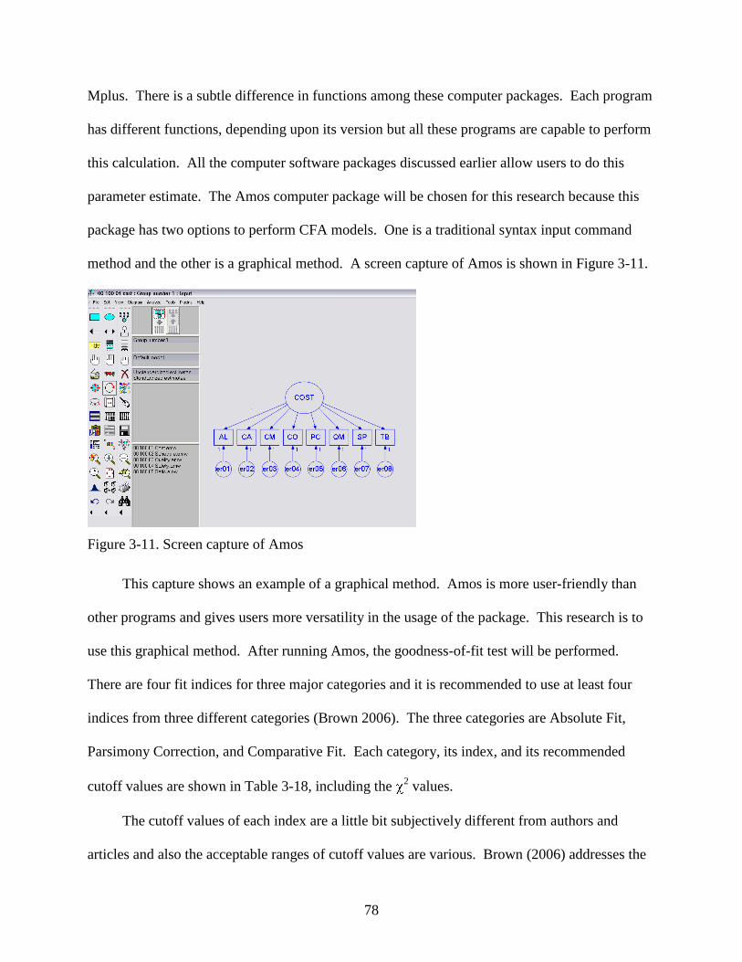
78
Mplus. There is a subtle difference in functions among these computer packages. Each program
has different functions, depending upon its version but all these programs are capable to perform
this calculation. All the computer software packages discussed earlier allow users to do this
parameter estimate. The Amos computer package will be chosen for this research because this
package has two options to perform CFA models. One is a traditional syntax input command
method and the other is a graphical method. A screen capture of Amos is shown in Figure 3-11.
Figure 3-11. Screen capture of Amos
This capture shows an example of a graphical method. Amos is more user-friendly than
other programs and gives users more versatility in the usage of the package. This research is to
use this graphical method. After running Amos, the goodness-of-fit test will be performed.
There are four fit indices for three major categories and it is recommended to use at least four
indices from three different categories (Brown 2006). The three categories are Absolute Fit,
Parsimony Correction, and Comparative Fit. Each category, its index, and its recommended
cutoff values are shown in Table 3-18, including the 2 values.
The cutoff values of each index are a little bit subjectively different from authors and
articles and also the acceptable ranges of cutoff values are various. Brown (2006) addresses the
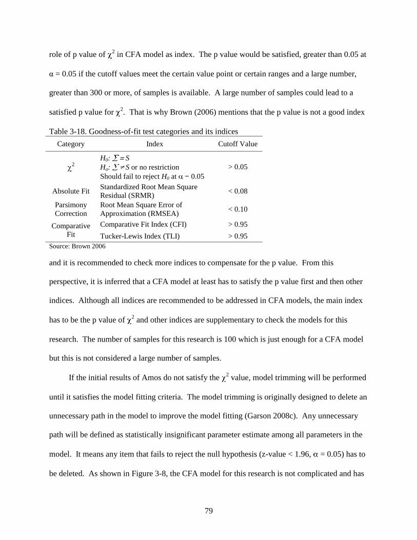
79
role of p value of 2 in CFA model as index. The p value would be satisfied, greater than 0.05 at
α = 0.05 if the cutoff values meet the certain value point or certain ranges and a large number,
greater than 300 or more, of samples is available. A large number of samples could lead to a
satisfied p value for 2. That is why Brown (2006) mentions that the p value is not a good index
Table 3-18. Goodness-of-fit test categories and its indices
Category Index Cutoff Value
2
H0: S
Ha: S or no restriction
Should fail to reject H0 at 0.05
> 0.05
Absolute Fit Standardized Root Mean Square
Residual (SRMR) < 0.08
Parsimony
Correction
Root Mean Square Error of
Approximation (RMSEA) < 0.10
Comparative
Fit
Comparative Fit Index (CFI) > 0.95
Tucker-Lewis Index (TLI) > 0.95
Source: Brown 2006
and it is recommended to check more indices to compensate for the p value. From this
perspective, it is inferred that a CFA model at least has to satisfy the p value first and then other
indices. Although all indices are recommended to be addressed in CFA models, the main index
has to be the p value of 2 and other indices are supplementary to check the models for this
research. The number of samples for this research is 100 which is just enough for a CFA model
but this is not considered a large number of samples.
If the initial results of Amos do not satisfy the 2 value, model trimming will be performed
until it satisfies the model fitting criteria. The model trimming is originally designed to delete an
unnecessary path in the model to improve the model fitting (Garson 2008c). Any unnecessary
path will be defined as statistically insignificant parameter estimate among all parameters in the
model. It means any item that fails to reject the null hypothesis (z-value < 1.96, = 0.05) has to
be deleted. As shown in Figure 3-8, the CFA model for this research is not complicated and has
80
a maximum of eight indicator variables. So the concept of model trimming is revised to delete
an item (variable) that is less significant than others in the model even though a parameter
estimate of that item is statistically significant. Model trimming will be performed until the final
revised model satisfies the goodness-of-fit test. A detailed method for deleting variables will be
addressed in Chapter 4.
Parameter estimate and significance test
In the previous section, the main concern was a CFA model fitting using the goodness-of-
fit test. This is a fitting for a whole model without testing for the statistical significance of an
individual variable. If a CFA model satisfies the goodness-of-fit test as a whole model, and then
the statistical significance test has to be performed for each individual remaining variable in the
model. During the model trimming process, some indicator variables may be deleted to satisfy
the goodness-of-fit test. For the remaining indicator variables, each parameter estimate has to be
checked. Even though there are some indicators remaining in the model after the model
trimming, there is a chance that any indicator may not be statistically significant at = 0.05.
The model cannot be finalized until the parameter estimate is completed. During this procedure,
the researcher could sort out the finalized indicators in the model and its parameter estimates.
All statistical significance test in this research is at = 0.05 unless specified otherwise.
In this chapter, all the strategies and design for this research have been laid out. Major
methodologies used for this research are 1) Canonical correlation for relationships between
problem groups; 2) EFA for the preliminary stage of CFA; and 3) CFA for the final model. This
chapter provides some detailed information on each method and the potential issues are already
addressed. Based on this information presented in this chapter, all the outputs of this research
will be discussed in Chapter 5, except for canonical correlations that were already discussed in

81
this chapter. In addition to methodologies presented in this chapter, the methodology for the
application of CFA outputs is Simple Multi-Attribute Rating Technique Using Swing Weight
(SMARTS). It is briefly reviewed in Chapter 2 and it will be discussed again in Chapter 5.
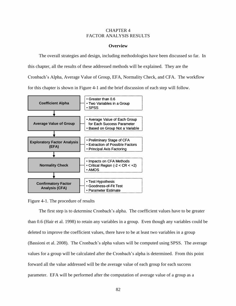
82
CHAPTER 4
FACTOR ANALYSIS RESULTS
Overview
The overall strategies and design, including methodologies have been discussed so far. In
this chapter, all the results of these addressed methods will be explained. They are the
Cronbach‟s Alpha, Average Value of Group, EFA, Normality Check, and CFA. The workflow
for this chapter is shown in Figure 4-1 and the brief discussion of each step will follow.
Coefficient Alpha• Greater than 0.6
• Two Variables in a Group• SPSS
Average Value of Group• Average Value of Each Group
for Each Success Parameter
• Based on Group Not a Variable
Exploratory Factor Analysis
(EFA)
• Preliminary Stage of CFA
• Extraction of Possible Factors
• Principal Axis Factoring
Normality Check• Impacts on CFA Methods• Critical Region (-2 < CR < +2)
• AMOS
Confirmatory Factor
Analysis (CFA)
• Test Hypothesis
• Goodness-of-Fit Test
• Parameter Estimate
Figure 4-1. The procedure of results
The first step is to determine Cronbach‟s alpha. The coefficient values have to be greater
than 0.6 (Hair et al. 1998) to retain any variables in a group. Even though any variables could be
deleted to improve the coefficient values, there have to be at least two variables in a group
(Bassioni et al. 2008). The Cronbach‟s alpha values will be computed using SPSS. The average
values for a group will be calculated after the Cronbach‟s alpha is determined. From this point
forward all the value addressed will be the average value of each group for each success
parameter. EFA will be performed after the computation of average value of a group as a
83
preliminary stage of CFA. This is a good process to check how many factors could be extracted
before CFA is performed. It will provide the overview of CFA. The method used for EFA is
principal axis factoring, using SPSS. The final stage of this chapter is to perform CFA. During
this stage, the hypotheses mentioned in Chapter 3 will be tested along with the goodness-of-fit
test and the parameter estimate. The program used for CFA is Amos.
Cronbach’s Alpha
Initial Cronbach’s Alpha Values
The initial Cronbach‟s alpha values are computed based on 43 problems groups. The
computation is completed for each group of each success parameter. There are eight groups
available for five different success parameters. This means that the computations will be done at
least 40 times (8 groups 5 success parameters). Table 3-1 Groups of Potential Problems
already addresses the number of variables (problems) in each group, so it is not necessary to
address it again here. The computation of Cronbach‟s alpha is done in SPSS. The rules
followed by the researcher in this portion of analysis were as follows:
It is necessary to retain as many problems as possible in a group for the computation of
average value and as many groups as it possible for the CFA models.
If the values of Cronbach‟s alpha meet the minimum (0.6), then all variables in a group are
retained. This rule is applied when the initial value satisfies the minimum and also the
coefficient value is greater than 0.6. In this case, all the variables will be retained because
the initial value already meets the minimum. If the initial Cronbach‟s alpha value is
smaller than the minimum, some problems are deleted.
The item deletion process will be stopped when the improved coefficient alpha value meets
the minimum.
The computations of coefficient alpha values are based on problems within each group but
the results are shown as group. There are eight problem groups available for each project
success parameter. If any of problem group does not meet the minimum Cronbach‟s alpha and
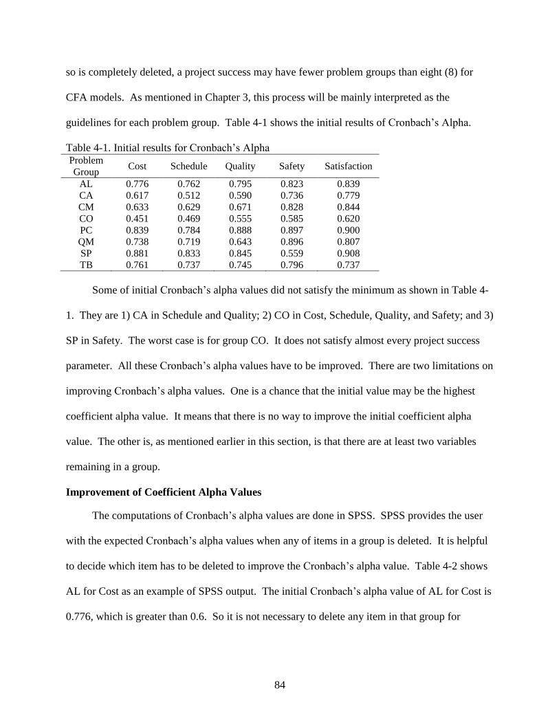
84
so is completely deleted, a project success may have fewer problem groups than eight (8) for
CFA models. As mentioned in Chapter 3, this process will be mainly interpreted as the
guidelines for each problem group. Table 4-1 shows the initial results of Cronbach‟s Alpha.
Table 4-1. Initial results for Cronbach‟s Alpha Problem
Group Cost Schedule Quality Safety Satisfaction
AL 0.776 0.762 0.795 0.823 0.839
CA 0.617 0.512 0.590 0.736 0.779
CM 0.633 0.629 0.671 0.828 0.844
CO 0.451 0.469 0.555 0.585 0.620
PC 0.839 0.784 0.888 0.897 0.900
QM 0.738 0.719 0.643 0.896 0.807
SP 0.881 0.833 0.845 0.559 0.908
TB 0.761 0.737 0.745 0.796 0.737
Some of initial Cronbach‟s alpha values did not satisfy the minimum as shown in Table 4-
1. They are 1) CA in Schedule and Quality; 2) CO in Cost, Schedule, Quality, and Safety; and 3)
SP in Safety. The worst case is for group CO. It does not satisfy almost every project success
parameter. All these Cronbach‟s alpha values have to be improved. There are two limitations on
improving Cronbach‟s alpha values. One is a chance that the initial value may be the highest
coefficient alpha value. It means that there is no way to improve the initial coefficient alpha
value. The other is, as mentioned earlier in this section, is that there are at least two variables
remaining in a group.
Improvement of Coefficient Alpha Values
The computations of Cronbach‟s alpha values are done in SPSS. SPSS provides the user
with the expected Cronbach‟s alpha values when any of items in a group is deleted. It is helpful
to decide which item has to be deleted to improve the Cronbach‟s alpha value. Table 4-2 shows
AL for Cost as an example of SPSS output. The initial Cronbach‟s alpha value of AL for Cost is
0.776, which is greater than 0.6. So it is not necessary to delete any item in that group for
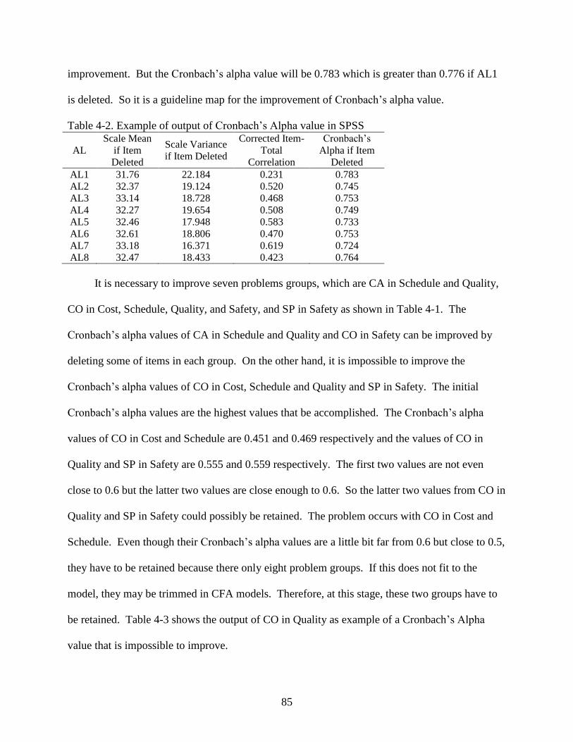
85
improvement. But the Cronbach‟s alpha value will be 0.783 which is greater than 0.776 if AL1
is deleted. So it is a guideline map for the improvement of Cronbach‟s alpha value.
Table 4-2. Example of output of Cronbach‟s Alpha value in SPSS
AL
Scale Mean
if Item
Deleted
Scale Variance
if Item Deleted
Corrected Item-
Total
Correlation
Cronbach‟s
Alpha if Item
Deleted
AL1 31.76 22.184 0.231 0.783
AL2 32.37 19.124 0.520 0.745
AL3 33.14 18.728 0.468 0.753
AL4 32.27 19.654 0.508 0.749
AL5 32.46 17.948 0.583 0.733
AL6 32.61 18.806 0.470 0.753
AL7 33.18 16.371 0.619 0.724
AL8 32.47 18.433 0.423 0.764
It is necessary to improve seven problems groups, which are CA in Schedule and Quality,
CO in Cost, Schedule, Quality, and Safety, and SP in Safety as shown in Table 4-1. The
Cronbach‟s alpha values of CA in Schedule and Quality and CO in Safety can be improved by
deleting some of items in each group. On the other hand, it is impossible to improve the
Cronbach‟s alpha values of CO in Cost, Schedule and Quality and SP in Safety. The initial
Cronbach‟s alpha values are the highest values that be accomplished. The Cronbach‟s alpha
values of CO in Cost and Schedule are 0.451 and 0.469 respectively and the values of CO in
Quality and SP in Safety are 0.555 and 0.559 respectively. The first two values are not even
close to 0.6 but the latter two values are close enough to 0.6. So the latter two values from CO in
Quality and SP in Safety could possibly be retained. The problem occurs with CO in Cost and
Schedule. Even though their Cronbach‟s alpha values are a little bit far from 0.6 but close to 0.5,
they have to be retained because there only eight problem groups. If this does not fit to the
model, they may be trimmed in CFA models. Therefore, at this stage, these two groups have to
be retained. Table 4-3 shows the output of CO in Quality as example of a Cronbach‟s Alpha
value that is impossible to improve.
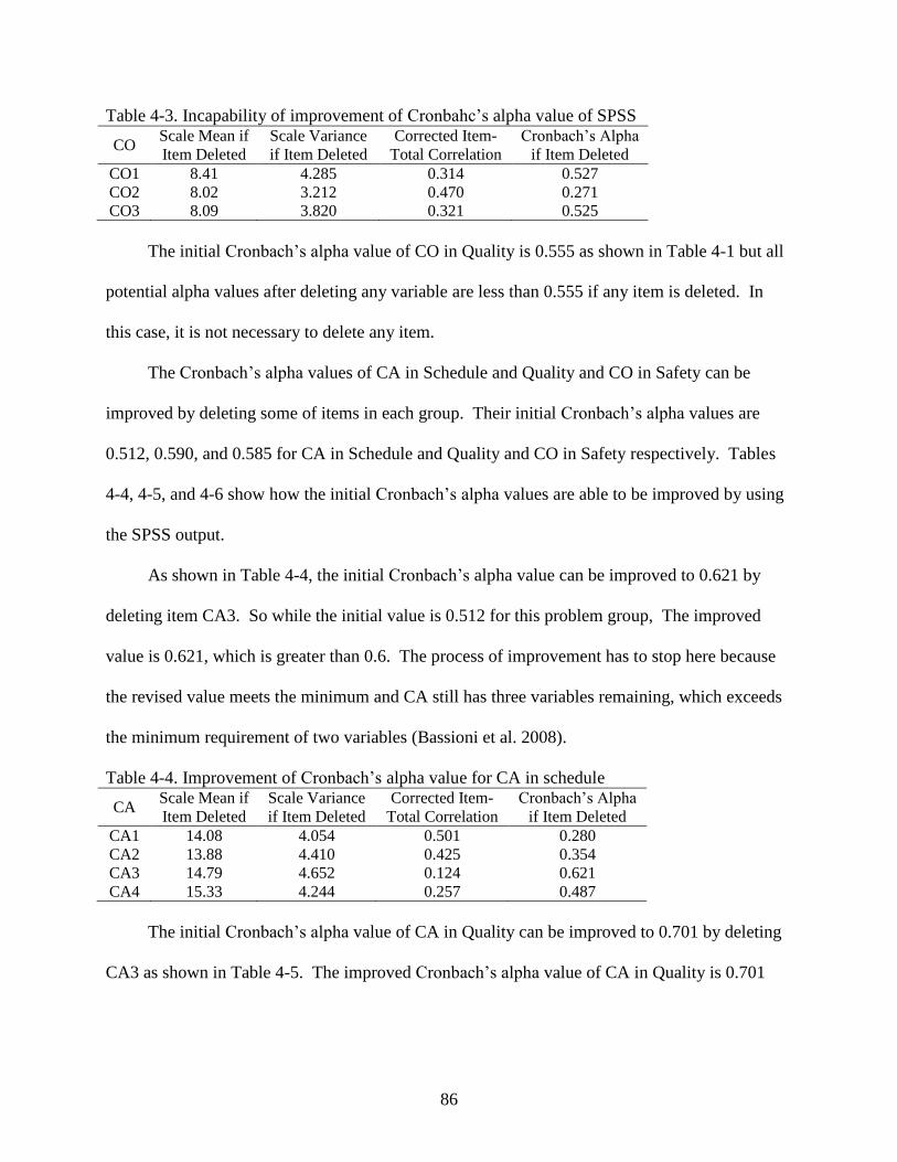
86
Table 4-3. Incapability of improvement of Cronbahc‟s alpha value of SPSS
CO Scale Mean if
Item Deleted
Scale Variance
if Item Deleted
Corrected Item-
Total Correlation
Cronbach‟s Alpha
if Item Deleted
CO1 8.41 4.285 0.314 0.527
CO2 8.02 3.212 0.470 0.271
CO3 8.09 3.820 0.321 0.525
The initial Cronbach‟s alpha value of CO in Quality is 0.555 as shown in Table 4-1 but all
potential alpha values after deleting any variable are less than 0.555 if any item is deleted. In
this case, it is not necessary to delete any item.
The Cronbach‟s alpha values of CA in Schedule and Quality and CO in Safety can be
improved by deleting some of items in each group. Their initial Cronbach‟s alpha values are
0.512, 0.590, and 0.585 for CA in Schedule and Quality and CO in Safety respectively. Tables
4-4, 4-5, and 4-6 show how the initial Cronbach‟s alpha values are able to be improved by using
the SPSS output.
As shown in Table 4-4, the initial Cronbach‟s alpha value can be improved to 0.621 by
deleting item CA3. So while the initial value is 0.512 for this problem group, The improved
value is 0.621, which is greater than 0.6. The process of improvement has to stop here because
the revised value meets the minimum and CA still has three variables remaining, which exceeds
the minimum requirement of two variables (Bassioni et al. 2008).
Table 4-4. Improvement of Cronbach‟s alpha value for CA in schedule
CA Scale Mean if
Item Deleted
Scale Variance
if Item Deleted
Corrected Item-
Total Correlation
Cronbach‟s Alpha
if Item Deleted
CA1 14.08 4.054 0.501 0.280
CA2 13.88 4.410 0.425 0.354
CA3 14.79 4.652 0.124 0.621
CA4 15.33 4.244 0.257 0.487
The initial Cronbach‟s alpha value of CA in Quality can be improved to 0.701 by deleting
CA3 as shown in Table 4-5. The improved Cronbach‟s alpha value of CA in Quality is 0.701
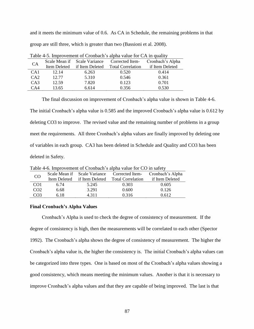
87
and it meets the minimum value of 0.6. As CA in Schedule, the remaining problems in that
group are still three, which is greater than two (Bassioni et al. 2008).
Table 4-5. Improvement of Cronbach‟s alpha value for CA in quality
CA Scale Mean if
Item Deleted
Scale Variance
if Item Deleted
Corrected Item-
Total Correlation
Cronbach‟s Alpha
if Item Deleted
CA1 12.14 6.263 0.520 0.414
CA2 12.77 5.310 0.546 0.361
CA3 12.59 7.820 0.123 0.701
CA4 13.65 6.614 0.356 0.530
The final discussion on improvement of Cronbach‟s alpha value is shown in Table 4-6.
The initial Cronbach‟s alpha value is 0.585 and the improved Cronbach‟s alpha value is 0.612 by
deleting CO3 to improve. The revised value and the remaining number of problems in a group
meet the requirements. All three Cronbach‟s alpha values are finally improved by deleting one
of variables in each group. CA3 has been deleted in Schedule and Quality and CO3 has been
deleted in Safety.
Table 4-6. Improvement of Cronbach‟s alpha value for CO in safety
CO Scale Mean if
Item Deleted
Scale Variance
if Item Deleted
Corrected Item-
Total Correlation
Cronbach‟s Alpha
if Item Deleted
CO1 6.74 5.245 0.303 0.605
CO2 6.68 3.291 0.600 0.126
CO3 6.18 4.311 0.316 0.612
Final Cronbach’s Alpha Values
Cronbach‟s Alpha is used to check the degree of consistency of measurement. If the
degree of consistency is high, then the measurements will be correlated to each other (Spector
1992). The Cronbach‟s alpha shows the degree of consistency of measurement. The higher the
Cronbach‟s alpha value is, the higher the consistency is. The initial Cronbach‟s alpha values can
be categorized into three types. One is based on most of the Cronbach‟s alpha values showing a
good consistency, which means meeting the minimum values. Another is that it is necessary to
improve Cronbach‟s alpha values and that they are capable of being improved. The last is that
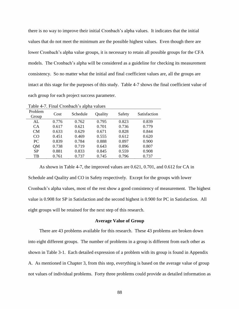
88
there is no way to improve their initial Cronbach‟s alpha values. It indicates that the initial
values that do not meet the minimum are the possible highest values. Even though there are
lower Cronbach‟s alpha value groups, it is necessary to retain all possible groups for the CFA
models. The Cronbach‟s alpha will be considered as a guideline for checking its measurement
consistency. So no matter what the initial and final coefficient values are, all the groups are
intact at this stage for the purposes of this study. Table 4-7 shows the final coefficient value of
each group for each project success parameter.
Table 4-7. Final Cronbach‟s alpha values Problem
Group Cost Schedule Quality Safety Satisfaction
AL 0.776 0.762 0.795 0.823 0.839
CA 0.617 0.621 0.701 0.736 0.779
CM 0.633 0.629 0.671 0.828 0.844
CO 0.451 0.469 0.555 0.612 0.620
PC 0.839 0.784 0.888 0.897 0.900
QM 0.738 0.719 0.643 0.896 0.807
SP 0.881 0.833 0.845 0.559 0.908
TB 0.761 0.737 0.745 0.796 0.737
As shown in Table 4-7, the improved values are 0.621, 0.701, and 0.612 for CA in
Schedule and Quality and CO in Safety respectively. Except for the groups with lower
Cronbach‟s alpha values, most of the rest show a good consistency of measurement. The highest
value is 0.908 for SP in Satisfaction and the second highest is 0.900 for PC in Satisfaction. All
eight groups will be retained for the next step of this research.
Average Value of Group
There are 43 problems available for this research. These 43 problems are broken down
into eight different groups. The number of problems in a group is different from each other as
shown in Table 3-1. Each detailed expression of a problem with its group is found in Appendix
A. As mentioned in Chapter 3, from this step, everything is based on the average value of group
not values of individual problems. Forty three problems could provide as detailed information as
89
possible but it is hard to provide an overview of problem group for each project success
parameter. One of the objectives of this research is to define the relationships between project
problems and their impacts on project success parameters. To achieve this goal, it is more
appropriate to use the average value of a group than to use the value of an individual problem,
especially dealing with multi-project success parameters. As discussed in Chapter 3, each
problem has a different impact on a success parameter such as frequency histogram and
canonical correlations. After studying the relationships between problems and project success
parameters, using the problem group perspective, then the individual level will be studied later
but not in this research because there is not enough data on the multi-project success parameter at
the problem group perspective. This research will provide an overview of the relationships
between problems and their impacts on project success parameters from the group level and will
be a first step for similar future studies.
Another reason for using the average value of a group is related to the method for CFA but
not for EFA. It is easier and more reliable to build a CFA model using eight groups than using
43 problems. So the average of each group value will be used for this research and everything
will be based on the group level and not on the individual problem. The deleted items like CA in
Schedule and Quality for improvement of the Cronbach‟s alpha value are excluded when the
computation of the average value is performed.
Exploratory Factor Analysis (EFA)
Overview
It is not a requirement to perform the EFA before the CFA is developed but it is a good
preliminary stage for CFA (Brown 2006; Thompson 2004). The theory or number of factors to
be tested could be assumed until the CFA is completed, for example, when only one factor is
expected for CFA. If there are two factors extracted using EFA, then CFA should be modified to
90
a two-factor model instead of one-factor model. On the other hand, if only one factor is
extracted by EFA, then the one-factor model will be tested in CFA. P value or other indices in
CFA represents how different the degree of gap between the raw data and the CFA model based
on a theory is. It will be statistically acceptable when the gap between the raw data and the CFA
model is small. That is why it is necessary and beneficial to perform EFA before CFA even
though it is not required. For this research, each success parameter is the expected factor
because every problem is evaluated in terms of its impact on each success parameter. If only one
factor is extracted, then it will be tested using CFA. If not, the model has to be modified. The
factor extraction method between EFA and CFA is similar. It means that there is a better chance
to get a small gap between the raw data and the CFA model.
Factor Extraction Technique
The factor extraction methods have been addressed in Chapter 3. The two methods are
Eigenvalue greater than 1.0 and the Scree test. There are mainly two techniques available in
EFA, they are principal component analysis (PCA) and common factor analysis (CFA). Both of
them are used for similar purposes of data reduction but the underlying assumptions are different
(ACITS 1995). In CFA the variance of each variable is decomposed into common variance that
is shared by other variables such as the factor variances in CFA (ACITS 1995). It means that it
considers only common variance and has a unique variance for each variable. On the other hand,
PCA considers the total variance, which is 1.0 and therefore, there is no distinction between
common and unique variance (ACITS 1995). Confirmatory factor analysis (CFA) is based on
the common factor analysis (CFA) model addressed in Chapter 3 (Floyd and Widaman 1995).
The purpose of EFA for this research is to facilitate the preliminary stage of CFA to explore the
construct in the data set. So the technique for EFA factor extraction has to be CFA not PCA.
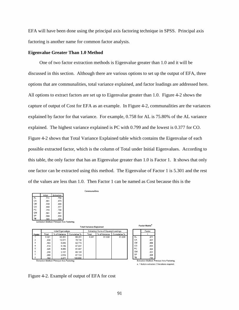
91
EFA will have been done using the principal axis factoring technique in SPSS. Principal axis
factoring is another name for common factor analysis.
Eigenvalue Greater Than 1.0 Method
One of two factor extraction methods is Eigenvalue greater than 1.0 and it will be
discussed in this section. Although there are various options to set up the output of EFA, three
options that are communalities, total variance explained, and factor loadings are addressed here.
All options to extract factors are set up to Eigenvalue greater than 1.0. Figure 4-2 shows the
capture of output of Cost for EFA as an example. In Figure 4-2, communalities are the variances
explained by factor for that variance. For example, 0.758 for AL is 75.80% of the AL variance
explained. The highest variance explained is PC with 0.799 and the lowest is 0.377 for CO.
Figure 4-2 shows that Total Variance Explained table which contains the Eigenvalue of each
possible extracted factor, which is the column of Total under Initial Eigenvalues. According to
this table, the only factor that has an Eigenvalue greater than 1.0 is Factor 1. It shows that only
one factor can be extracted using this method. The Eigenvalue of Factor 1 is 5.301 and the rest
of the values are less than 1.0. Then Factor 1 can be named as Cost because this is the
Figure 4-2. Example of output of EFA for cost
92
measurement of problem impacts on cost and the only factor extracted. The column of % of
Variance shows that the variance explained by that factor out of all potential factors. The Factor
1 is the highest with 66.261% and the second highest is factor 2 with 10.477%. The first
extracted factor has the highest Eigenvalue and highest % variance explained and the last
extracted factor has the lowest Eigenvalue and lowest % variance explained. This is a partial
explanation of why the Eigenvalue has to be greater than 1.0.
The last table in Figure 4-2 shows the factor loading of each variable for the extracted
factor, called Factor Matrix. The highest factor loading comes from PC with 0.894 and the
lowest loading comes from 0.614. Form this table, it is evident that PC has the highest impact on
Cost and CO has the lowest impact on Cost. So from this example, only one factor is extracted
in Cost with 66.261% of variance explained. The rest of project success parameters, Schedule,
Quality, Safety, and Satisfaction, will be as analyzed similarly to the way Cost has been done.
Table 4-8 shows the EFA output summary for Schedule using SPSS.
Table 4-8. EFA summary output of schedule
Factor Eigenvalues
Factor Loading Total % of Variance Cumulative %
1 5.249 65.616 65.616 AL 0.861
2 0.657 8.208 73.825 CA 0.657
3 0.495 6.191 80.016 CM 0.791
4 0.471 5.889 85.905 CO 0.690
5 0.433 5.418 91.323 PC 0.766
6 0.292 3.655 94.928 QM 0.814
7 0.224 2.795 97.772 SP 0.788
8 0.178 2.228 100.000 TB 0.854
The number of extracted factor using the Eigenvalue greater than 1.0 method is one for
Schedule as shown Table 4-8. Only one factor (Factor 1 in Table 4-8) is extracted with an
Eigenvalue of 5.249 and its communality (% of variance) is 65.616%. The extracted factor
would be named as Schedule because only one factor is extracted and this is a measurement
about Schedule. The two columns on the right show the extracted factor‟s factor loading. The
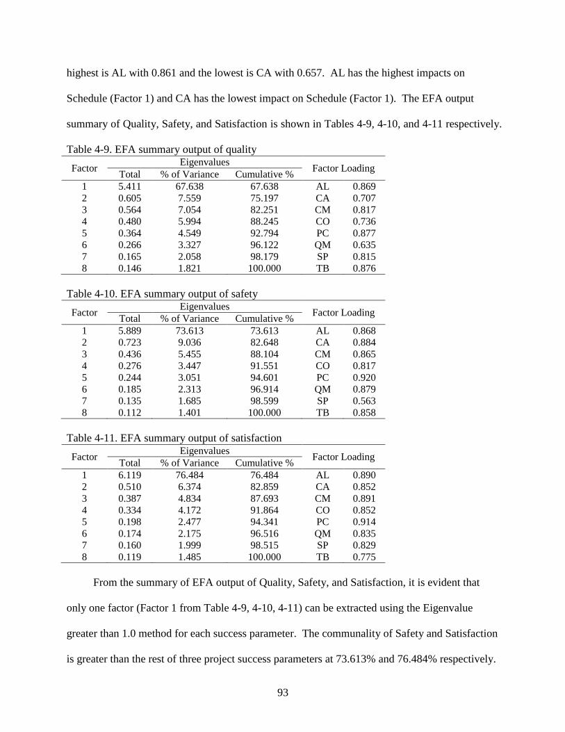
93
highest is AL with 0.861 and the lowest is CA with 0.657. AL has the highest impacts on
Schedule (Factor 1) and CA has the lowest impact on Schedule (Factor 1). The EFA output
summary of Quality, Safety, and Satisfaction is shown in Tables 4-9, 4-10, and 4-11 respectively.
Table 4-9. EFA summary output of quality
Factor Eigenvalues
Factor Loading Total % of Variance Cumulative %
1 5.411 67.638 67.638 AL 0.869
2 0.605 7.559 75.197 CA 0.707
3 0.564 7.054 82.251 CM 0.817
4 0.480 5.994 88.245 CO 0.736
5 0.364 4.549 92.794 PC 0.877
6 0.266 3.327 96.122 QM 0.635
7 0.165 2.058 98.179 SP 0.815
8 0.146 1.821 100.000 TB 0.876
Table 4-10. EFA summary output of safety
Factor Eigenvalues
Factor Loading Total % of Variance Cumulative %
1 5.889 73.613 73.613 AL 0.868
2 0.723 9.036 82.648 CA 0.884
3 0.436 5.455 88.104 CM 0.865
4 0.276 3.447 91.551 CO 0.817
5 0.244 3.051 94.601 PC 0.920
6 0.185 2.313 96.914 QM 0.879
7 0.135 1.685 98.599 SP 0.563
8 0.112 1.401 100.000 TB 0.858
Table 4-11. EFA summary output of satisfaction
Factor Eigenvalues
Factor Loading Total % of Variance Cumulative %
1 6.119 76.484 76.484 AL 0.890
2 0.510 6.374 82.859 CA 0.852
3 0.387 4.834 87.693 CM 0.891
4 0.334 4.172 91.864 CO 0.852
5 0.198 2.477 94.341 PC 0.914
6 0.174 2.175 96.516 QM 0.835
7 0.160 1.999 98.515 SP 0.829
8 0.119 1.485 100.000 TB 0.775
From the summary of EFA output of Quality, Safety, and Satisfaction, it is evident that
only one factor (Factor 1 from Table 4-9, 4-10, 4-11) can be extracted using the Eigenvalue
greater than 1.0 method for each success parameter. The communality of Safety and Satisfaction
is greater than the rest of three project success parameters at 73.613% and 76.484% respectively.
94
The highest factor loading among three project success parameters comes from PC with 0.877,
0.920, and 0.914 for Quality, Safety, and Satisfaction respectively and the lowest factor loadings
among them are different from each other. Even though PC has the highest impact on these three
success parameters, the rest of project problem group has different factor loadings on each
success parameter. It is clearly shown that each problem group has a different impact on a
project success parameter. Using the Eigenvalue greater than 1.0 method, only one factor from
each project success parameter could be extracted. As Thompson (2004) indicated no cases exist
of Eigenvalues that are right above 1.0 like 1.002 or 1.001 and right below 1.0 like 0.998 or
0.995 when using this method for factor selection. All five project success parameters have clear
cutoff Eigenvalues for their factor selection.
Scree Test Method
The Eigenvalues depicts the amount of information represented within a given factor
(Thompson 2004). The first extracted factor has the highest Eigenvalue and the last extracted
factor has the lowest Eigenvalue. “Scree is the rubble of loose rock and boulders not solidly
attached to mountains that collects at the feet of the mountains. Cattell thought of solid, big,
intact mountains as being analogous to solid, noteworthy factors that researchers should
recognize and retain. Trivial factors, however, are analogous to Scree, and should be left behind
in the extraction process” (Thompson 2004). Trivial factors show the trend of flattening of
slopes in the graph of Eigenvalues and factors. Scree test looks for a spot at where the slope of
line starts flattening or changes drastically, such as an elbow, because after the slope changes
significantly, there is no big difference in slope among factors. It represents that these are the
trivial factors such as Scree in the mountains. Table 4-12 shows the summary of Eigenvalues for
all possible factors of each success parameter. The Scree plot for each success parameter will be
drawn based on the Eigenvalues shown in Table 4-12. The difference in Eigenvalues between
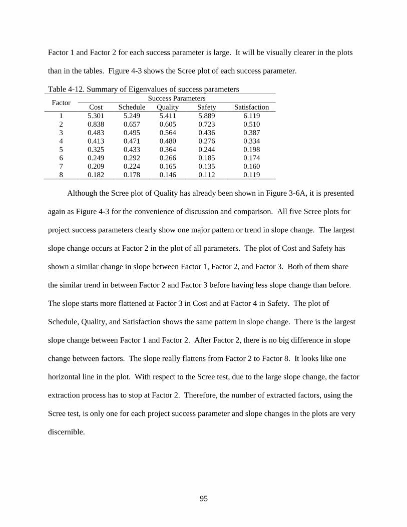
95
Factor 1 and Factor 2 for each success parameter is large. It will be visually clearer in the plots
than in the tables. Figure 4-3 shows the Scree plot of each success parameter.
Table 4-12. Summary of Eigenvalues of success parameters
Factor Success Parameters
Cost Schedule Quality Safety Satisfaction
1 5.301 5.249 5.411 5.889 6.119
2 0.838 0.657 0.605 0.723 0.510
3 0.483 0.495 0.564 0.436 0.387
4 0.413 0.471 0.480 0.276 0.334
5 0.325 0.433 0.364 0.244 0.198
6 0.249 0.292 0.266 0.185 0.174
7 0.209 0.224 0.165 0.135 0.160
8 0.182 0.178 0.146 0.112 0.119
Although the Scree plot of Quality has already been shown in Figure 3-6A, it is presented
again as Figure 4-3 for the convenience of discussion and comparison. All five Scree plots for
project success parameters clearly show one major pattern or trend in slope change. The largest
slope change occurs at Factor 2 in the plot of all parameters. The plot of Cost and Safety has
shown a similar change in slope between Factor 1, Factor 2, and Factor 3. Both of them share
the similar trend in between Factor 2 and Factor 3 before having less slope change than before.
The slope starts more flattened at Factor 3 in Cost and at Factor 4 in Safety. The plot of
Schedule, Quality, and Satisfaction shows the same pattern in slope change. There is the largest
slope change between Factor 1 and Factor 2. After Factor 2, there is no big difference in slope
change between factors. The slope really flattens from Factor 2 to Factor 8. It looks like one
horizontal line in the plot. With respect to the Scree test, due to the large slope change, the factor
extraction process has to stop at Factor 2. Therefore, the number of extracted factors, using the
Scree test, is only one for each project success parameter and slope changes in the plots are very
discernible.
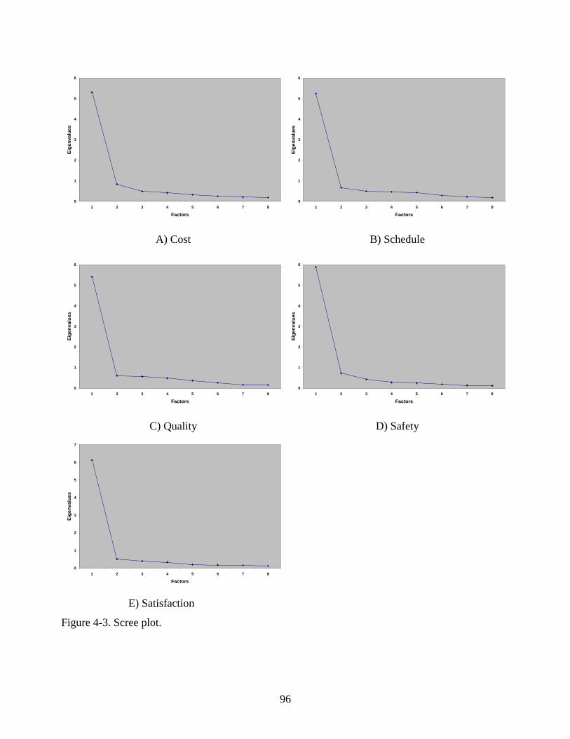
96
0
1
2
3
4
5
6
1 2 3 4 5 6 7 8
Factors
Eig
en
va
lue
s
0
1
2
3
4
5
6
1 2 3 4 5 6 7 8
Factors
Eig
en
va
lue
s
A) Cost B) Schedule
0
1
2
3
4
5
6
1 2 3 4 5 6 7 8
Factors
Eig
en
va
lue
s
0
1
2
3
4
5
6
1 2 3 4 5 6 7 8
Factors
Eig
en
va
lue
s
C) Quality D) Safety
0
1
2
3
4
5
6
7
1 2 3 4 5 6 7 8
Factors
Eig
en
va
lue
s
E) Satisfaction
Figure 4-3. Scree plot.
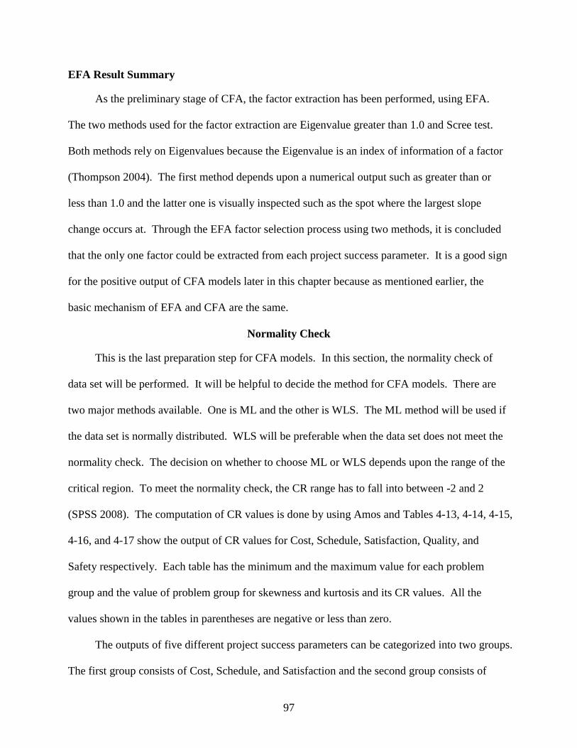
97
EFA Result Summary
As the preliminary stage of CFA, the factor extraction has been performed, using EFA.
The two methods used for the factor extraction are Eigenvalue greater than 1.0 and Scree test.
Both methods rely on Eigenvalues because the Eigenvalue is an index of information of a factor
(Thompson 2004). The first method depends upon a numerical output such as greater than or
less than 1.0 and the latter one is visually inspected such as the spot where the largest slope
change occurs at. Through the EFA factor selection process using two methods, it is concluded
that the only one factor could be extracted from each project success parameter. It is a good sign
for the positive output of CFA models later in this chapter because as mentioned earlier, the
basic mechanism of EFA and CFA are the same.
Normality Check
This is the last preparation step for CFA models. In this section, the normality check of
data set will be performed. It will be helpful to decide the method for CFA models. There are
two major methods available. One is ML and the other is WLS. The ML method will be used if
the data set is normally distributed. WLS will be preferable when the data set does not meet the
normality check. The decision on whether to choose ML or WLS depends upon the range of the
critical region. To meet the normality check, the CR range has to fall into between -2 and 2
(SPSS 2008). The computation of CR values is done by using Amos and Tables 4-13, 4-14, 4-15,
4-16, and 4-17 show the output of CR values for Cost, Schedule, Satisfaction, Quality, and
Safety respectively. Each table has the minimum and the maximum value for each problem
group and the value of problem group for skewness and kurtosis and its CR values. All the
values shown in the tables in parentheses are negative or less than zero.
The outputs of five different project success parameters can be categorized into two groups.
The first group consists of Cost, Schedule, and Satisfaction and the second group consists of
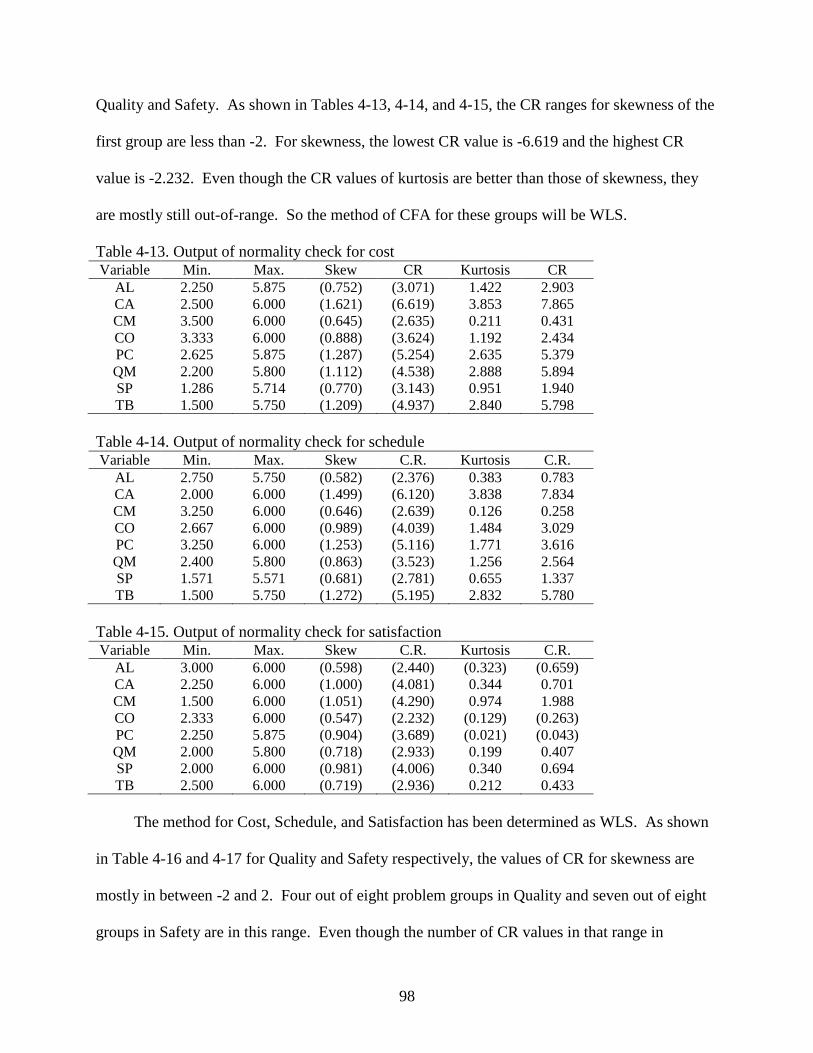
98
Quality and Safety. As shown in Tables 4-13, 4-14, and 4-15, the CR ranges for skewness of the
first group are less than -2. For skewness, the lowest CR value is -6.619 and the highest CR
value is -2.232. Even though the CR values of kurtosis are better than those of skewness, they
are mostly still out-of-range. So the method of CFA for these groups will be WLS.
Table 4-13. Output of normality check for cost Variable Min. Max. Skew CR Kurtosis CR
AL 2.250 5.875 (0.752) (3.071) 1.422 2.903
CA 2.500 6.000 (1.621) (6.619) 3.853 7.865
CM 3.500 6.000 (0.645) (2.635) 0.211 0.431
CO 3.333 6.000 (0.888) (3.624) 1.192 2.434
PC 2.625 5.875 (1.287) (5.254) 2.635 5.379
QM 2.200 5.800 (1.112) (4.538) 2.888 5.894
SP 1.286 5.714 (0.770) (3.143) 0.951 1.940
TB 1.500 5.750 (1.209) (4.937) 2.840 5.798
Table 4-14. Output of normality check for schedule Variable Min. Max. Skew C.R. Kurtosis C.R.
AL 2.750 5.750 (0.582) (2.376) 0.383 0.783
CA 2.000 6.000 (1.499) (6.120) 3.838 7.834
CM 3.250 6.000 (0.646) (2.639) 0.126 0.258
CO 2.667 6.000 (0.989) (4.039) 1.484 3.029
PC 3.250 6.000 (1.253) (5.116) 1.771 3.616
QM 2.400 5.800 (0.863) (3.523) 1.256 2.564
SP 1.571 5.571 (0.681) (2.781) 0.655 1.337
TB 1.500 5.750 (1.272) (5.195) 2.832 5.780
Table 4-15. Output of normality check for satisfaction Variable Min. Max. Skew C.R. Kurtosis C.R.
AL 3.000 6.000 (0.598) (2.440) (0.323) (0.659)
CA 2.250 6.000 (1.000) (4.081) 0.344 0.701
CM 1.500 6.000 (1.051) (4.290) 0.974 1.988
CO 2.333 6.000 (0.547) (2.232) (0.129) (0.263)
PC 2.250 5.875 (0.904) (3.689) (0.021) (0.043)
QM 2.000 5.800 (0.718) (2.933) 0.199 0.407
SP 2.000 6.000 (0.981) (4.006) 0.340 0.694
TB 2.500 6.000 (0.719) (2.936) 0.212 0.433
The method for Cost, Schedule, and Satisfaction has been determined as WLS. As shown
in Table 4-16 and 4-17 for Quality and Safety respectively, the values of CR for skewness are
mostly in between -2 and 2. Four out of eight problem groups in Quality and seven out of eight
groups in Safety are in this range. Even though the number of CR values in that range in
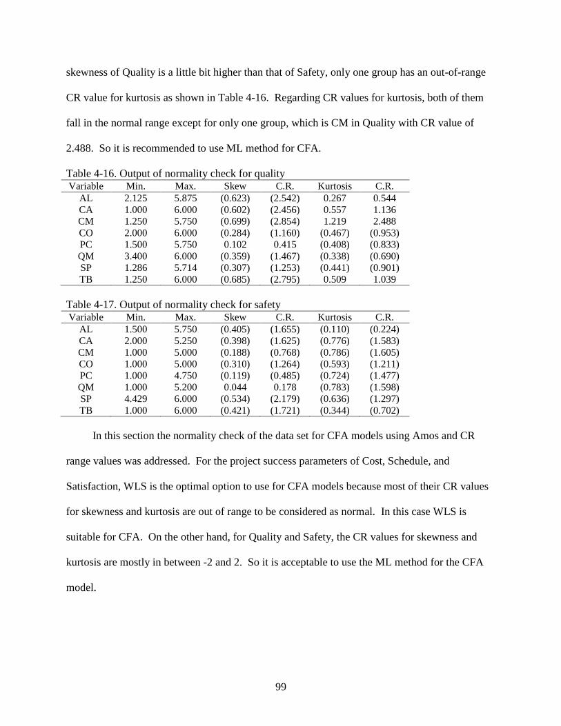
99
skewness of Quality is a little bit higher than that of Safety, only one group has an out-of-range
CR value for kurtosis as shown in Table 4-16. Regarding CR values for kurtosis, both of them
fall in the normal range except for only one group, which is CM in Quality with CR value of
2.488. So it is recommended to use ML method for CFA.
Table 4-16. Output of normality check for quality Variable Min. Max. Skew C.R. Kurtosis C.R.
AL 2.125 5.875 (0.623) (2.542) 0.267 0.544
CA 1.000 6.000 (0.602) (2.456) 0.557 1.136
CM 1.250 5.750 (0.699) (2.854) 1.219 2.488
CO 2.000 6.000 (0.284) (1.160) (0.467) (0.953)
PC 1.500 5.750 0.102 0.415 (0.408) (0.833)
QM 3.400 6.000 (0.359) (1.467) (0.338) (0.690)
SP 1.286 5.714 (0.307) (1.253) (0.441) (0.901)
TB 1.250 6.000 (0.685) (2.795) 0.509 1.039
Table 4-17. Output of normality check for safety Variable Min. Max. Skew C.R. Kurtosis C.R.
AL 1.500 5.750 (0.405) (1.655) (0.110) (0.224)
CA 2.000 5.250 (0.398) (1.625) (0.776) (1.583)
CM 1.000 5.000 (0.188) (0.768) (0.786) (1.605)
CO 1.000 5.000 (0.310) (1.264) (0.593) (1.211)
PC 1.000 4.750 (0.119) (0.485) (0.724) (1.477)
QM 1.000 5.200 0.044 0.178 (0.783) (1.598)
SP 4.429 6.000 (0.534) (2.179) (0.636) (1.297)
TB 1.000 6.000 (0.421) (1.721) (0.344) (0.702)
In this section the normality check of the data set for CFA models using Amos and CR
range values was addressed. For the project success parameters of Cost, Schedule, and
Satisfaction, WLS is the optimal option to use for CFA models because most of their CR values
for skewness and kurtosis are out of range to be considered as normal. In this case WLS is
suitable for CFA. On the other hand, for Quality and Safety, the CR values for skewness and
kurtosis are mostly in between -2 and 2. So it is acceptable to use the ML method for the CFA
model.
100
Confirmatory Factor Analysis (CFA)
Overview
All the procedures addressed in this chapter so far were in preparation for this section. The
Cronbach‟s alpha values have shown the consistency of the data and some of items were deleted
to improve the Cronbach‟s alpha values. Based on the results of Cronbach‟s alpha, EFA has
been performed to extract possible factors before CFA, using the Eigenvalue greater than 1.0 and
Scree test method. Outputs of EFA support one factor model for the equivalent CFA model of
each project success parameter. Finally, the normality check of data helps decide the method for
CFA models like WLS for Cost, Schedule, and Satisfaction and ML for Quality and Safety. The
main focus of this section is how well a latent factor (each project success parameter) is
manifested by eight problem groups. If they are, then what is the degree of impact of each
problem group on each success parameter? If not, how many problem groups are related to a
latent factor? And then what are the impacts of each related problem group on each success
parameter? In this section, the more detailed information on CFA models will be discussed in the
following order: interpretation of the parameter estimate process; initial results; model trimming,
and final results.
Interpretation of Parameter Estimate Process
There are two terminologies available for any CFA model in the parameter estimate
process. One is the raw estimate and the other is the standard estimate. All the parameter
estimates found in articles are normally standard estimated (Garson 2008c). The difference
between a raw estimate and a standard estimate is the base. The raw estimate is based on one of
variables in the model and the standard estimate is based on the latent factor. The mechanism for
computation of the parameter estimate is to compute the raw estimate first and then the raw
estimate will be converted into standard estimate. Each unique variance will be computed based
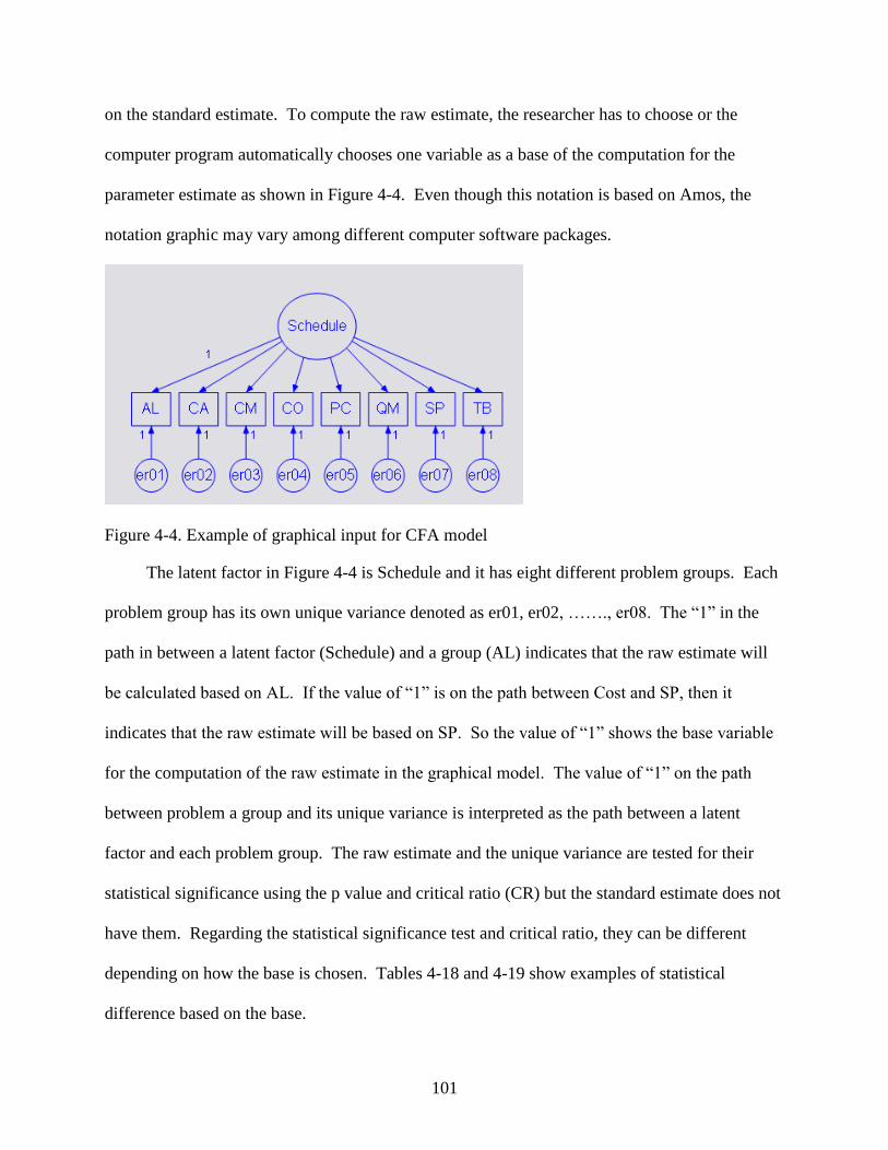
101
on the standard estimate. To compute the raw estimate, the researcher has to choose or the
computer program automatically chooses one variable as a base of the computation for the
parameter estimate as shown in Figure 4-4. Even though this notation is based on Amos, the
notation graphic may vary among different computer software packages.
Figure 4-4. Example of graphical input for CFA model
The latent factor in Figure 4-4 is Schedule and it has eight different problem groups. Each
problem group has its own unique variance denoted as er01, er02, ……., er08. The “1” in the
path in between a latent factor (Schedule) and a group (AL) indicates that the raw estimate will
be calculated based on AL. If the value of “1” is on the path between Cost and SP, then it
indicates that the raw estimate will be based on SP. So the value of “1” shows the base variable
for the computation of the raw estimate in the graphical model. The value of “1” on the path
between problem a group and its unique variance is interpreted as the path between a latent
factor and each problem group. The raw estimate and the unique variance are tested for their
statistical significance using the p value and critical ratio (CR) but the standard estimate does not
have them. Regarding the statistical significance test and critical ratio, they can be different
depending on how the base is chosen. Tables 4-18 and 4-19 show examples of statistical
difference based on the base.
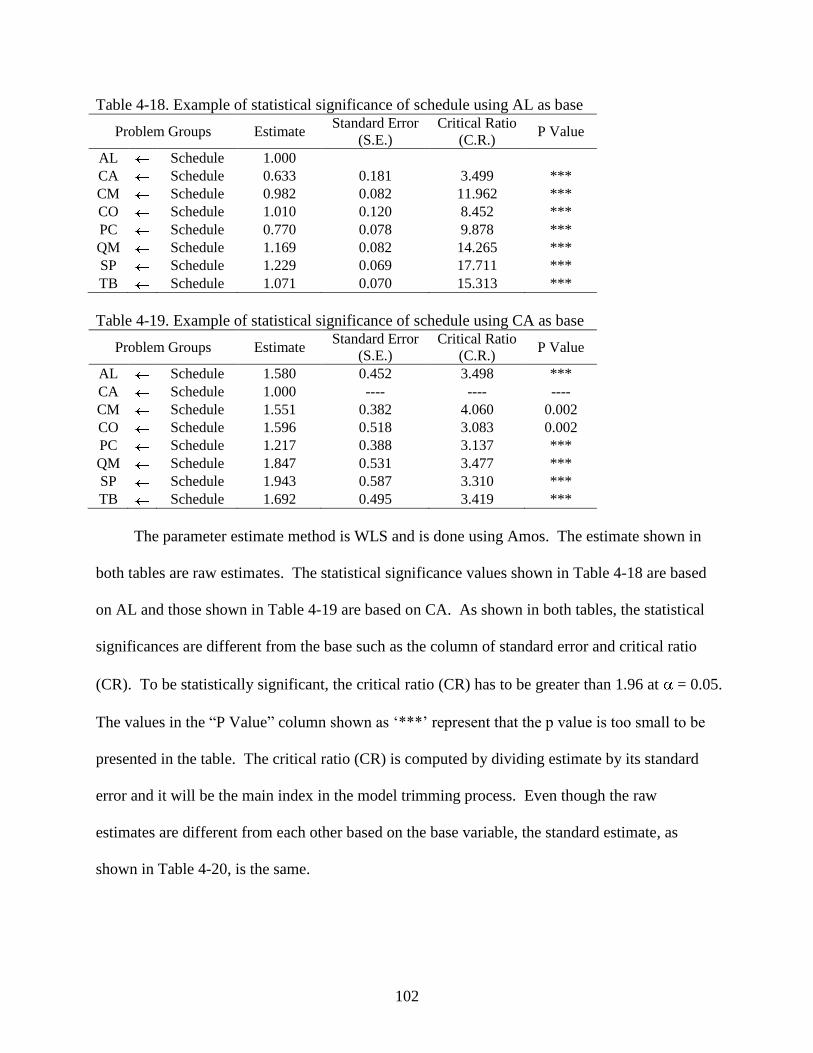
102
Table 4-18. Example of statistical significance of schedule using AL as base
Problem Groups Estimate Standard Error
(S.E.)
Critical Ratio
(C.R.) P Value
AL Schedule 1.000
CA Schedule 0.633 0.181 3.499 ***
CM Schedule 0.982 0.082 11.962 ***
CO Schedule 1.010 0.120 8.452 ***
PC Schedule 0.770 0.078 9.878 ***
QM Schedule 1.169 0.082 14.265 ***
SP Schedule 1.229 0.069 17.711 ***
TB Schedule 1.071 0.070 15.313 ***
Table 4-19. Example of statistical significance of schedule using CA as base
Problem Groups Estimate Standard Error
(S.E.)
Critical Ratio
(C.R.) P Value
AL Schedule 1.580 0.452 3.498 ***
CA Schedule 1.000 ---- ---- ----
CM Schedule 1.551 0.382 4.060 0.002
CO Schedule 1.596 0.518 3.083 0.002
PC Schedule 1.217 0.388 3.137 ***
QM Schedule 1.847 0.531 3.477 ***
SP Schedule 1.943 0.587 3.310 ***
TB Schedule 1.692 0.495 3.419 ***
The parameter estimate method is WLS and is done using Amos. The estimate shown in
both tables are raw estimates. The statistical significance values shown in Table 4-18 are based
on AL and those shown in Table 4-19 are based on CA. As shown in both tables, the statistical
significances are different from the base such as the column of standard error and critical ratio
(CR). To be statistically significant, the critical ratio (CR) has to be greater than 1.96 at = 0.05.
The values in the “P Value” column shown as „***‟ represent that the p value is too small to be
presented in the table. The critical ratio (CR) is computed by dividing estimate by its standard
error and it will be the main index in the model trimming process. Even though the raw
estimates are different from each other based on the base variable, the standard estimate, as
shown in Table 4-20, is the same.
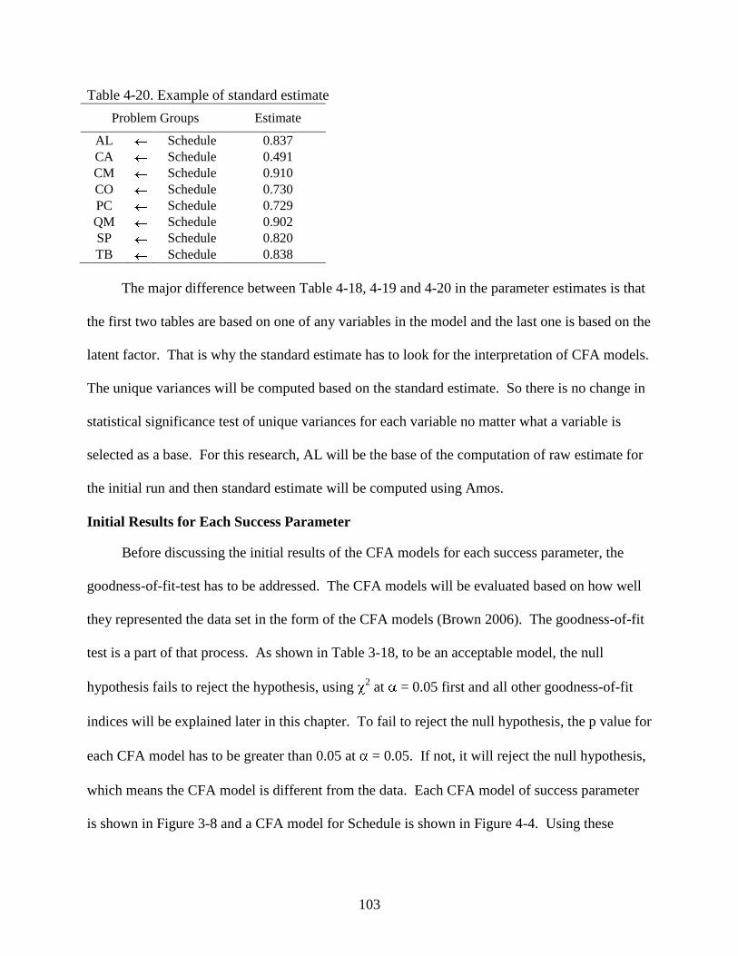
103
Table 4-20. Example of standard estimate
Problem Groups Estimate
AL Schedule 0.837
CA Schedule 0.491
CM Schedule 0.910
CO Schedule 0.730
PC Schedule 0.729
QM Schedule 0.902
SP Schedule 0.820
TB Schedule 0.838
The major difference between Table 4-18, 4-19 and 4-20 in the parameter estimates is that
the first two tables are based on one of any variables in the model and the last one is based on the
latent factor. That is why the standard estimate has to look for the interpretation of CFA models.
The unique variances will be computed based on the standard estimate. So there is no change in
statistical significance test of unique variances for each variable no matter what a variable is
selected as a base. For this research, AL will be the base of the computation of raw estimate for
the initial run and then standard estimate will be computed using Amos.
Initial Results for Each Success Parameter
Before discussing the initial results of the CFA models for each success parameter, the
goodness-of-fit-test has to be addressed. The CFA models will be evaluated based on how well
they represented the data set in the form of the CFA models (Brown 2006). The goodness-of-fit
test is a part of that process. As shown in Table 3-18, to be an acceptable model, the null
hypothesis fails to reject the hypothesis, using 2 at = 0.05 first and all other goodness-of-fit
indices will be explained later in this chapter. To fail to reject the null hypothesis, the p value for
each CFA model has to be greater than 0.05 at = 0.05. If not, it will reject the null hypothesis,
which means the CFA model is different from the data. Each CFA model of success parameter
is shown in Figure 3-8 and a CFA model for Schedule is shown in Figure 4-4. Using these
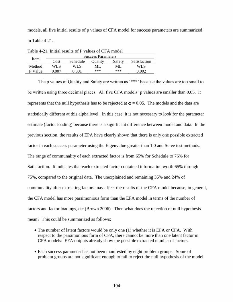
104
models, all five initial results of p values of CFA model for success parameters are summarized
in Table 4-21.
Table 4-21. Initial results of P values of CFA model
Item Success Parameters
Cost Schedule Quality Safety Satisfaction
Method WLS WLS ML ML WLS
P Value 0.007 0.001 *** *** 0.002
The p values of Quality and Safety are written as „***‟ because the values are too small to
be written using three decimal places. All five CFA models‟ p values are smaller than 0.05. It
represents that the null hypothesis has to be rejected at = 0.05. The models and the data are
statistically different at this alpha level. In this case, it is not necessary to look for the parameter
estimate (factor loading) because there is a significant difference between model and data. In the
previous section, the results of EPA have clearly shown that there is only one possible extracted
factor in each success parameter using the Eigenvalue greater than 1.0 and Scree test methods.
The range of communality of each extracted factor is from 65% for Schedule to 76% for
Satisfaction. It indicates that each extracted factor contained information worth 65% through
75%, compared to the original data. The unexplained and remaining 35% and 24% of
communality after extracting factors may affect the results of the CFA model because, in general,
the CFA model has more parsimonious form than the EFA model in terms of the number of
factors and factor loadings, etc (Brown 2006). Then what does the rejection of null hypothesis
mean? This could be summarized as follows:
The number of latent factors would be only one (1) whether it is EFA or CFA. With
respect to the parsimonious form of CFA, there cannot be more than one latent factor in
CFA models. EFA outputs already show the possible extracted number of factors.
Each success parameter has not been manifested by eight problem groups. Some of
problem groups are not significant enough to fail to reject the null hypothesis of the model.
105
The main hypothesis of this research addressed in the previous section is that “Each
success parameter is manifested by eight problem groups” and, according to the summary above,
this hypothesis has to be rejected for all five project success parameters. It indicates that each
project success parameter has some problem groups, which are less consistent than the others on
the degree of impact using CFA models. It is another benefit of the usage of CFA models to
choose better variables. It is sometimes hard to select some variables among a group of variables
in a reasonable way. The average value and ranking by summation could be used the most for
the selection, but the cutoff values or the range will be based on the personal or groups opinion
to choose. In terms of this, the CFA model is useful to filter the variables.
From the discussion above, all p values make the null hypothesis rejected for five CFA
models. It is evident that each project parameter has not been manifested by eight problem
groups. It is necessary to trim the CFA models to find the variables that are more consistent than
others among the eight problem groups in satisfying the statistical significance test.
CFA Model Trimming
Overview
As mentioned earlier, it is necessary to trim the CFA models. This process will be a
filtering process to find any problem groups that affect the failure to reject the null hypothesis
and also be a process to choose the best fitted model for each success parameter. Those problem
groups will be removed from the CFA models. There are two ways to find out the best-fitted
model. One is using critical ratio (CR) and the other is using a combination of each problem
group to form a model with less than eight variables per CFA model.
Garson (2008c) addresses the usage of critical ratio (CR) for improvement of model fitting.
Deleting a statistically insignificant path in the model can improve the model fitting. The value
of the critical ratio (CR) is found by dividing the parameter estimate by its standard error. The
106
cutoff value is 1.96 at = 0.05. Any paths with critical ratio (CR) value less than 1.96 will be
removed from the model. But for this research, the CFA models are not that complicated and
have only a maximum of eight variables for each success parameter. So this concept will be
revised as deleting any variables that are statistically insignificant or less significant than others
when all variables are significant until the null hypothesis fails to be rejected. But the critical
ratio (CR) will change depending upon what base is set up for each model as shown in Tables 4-
18 and 4-19. So the critical ratio (CR) method will be performed, using eight possible models
for each success parameter and each model will have a different base. The other method is
generating all possible combinations of problem groups consisting of seven variables or less in
the model until the null hypothesis fails to be rejected. The first method is deleting any variables
in the model to improve model fit. On the other hand, the second method is to find the best fitted
model using all possible combinations of problem groups. Since the CFA model for the eight
problem groups fails to be rejected, the maximum number of problem groups in the model will
be seven. Due to the all possible number of combination models for seven or less problem group
for each CFA model, this is a time consuming process, compared to the critical ration (CR)
method. For example there are eight possible combinations that consist of seven problem groups
for each success parameter and there are 28 possible combinations that consist of six problem
groups for each success parameter. A combination of six problem groups will be performed only
if there is no best fitted model within seven problem groups of combination. A total number of
combinations of five problem groups for each success parameter will have more than those of the
seven and six problem groups.
Deleting any variables in the model will stop when the p value is greater than 0.05 in a
different base model, using the critical ratio (CR) method. All combination methods will
107
generate all possible models with the seven problem groups first, and then six problem groups
only if there is no combination to meet the p value greater than 0.05 with seven problem groups.
The selection of best-fitted model for both methods is based on the p value and number of
problem groups retained in the model. In the best-fitted model selection, the first priority among
fitted models is any model with the highest p value and the largest number of problem groups
retained. The second priority is any model with the minimum satisfied p value and the largest
number of problem groups retained. For example, there are two models available having the
same p value but a different number of problem groups retained. One has seven problem groups
and the other has six problem groups in the model. Then the best-fitted model would be the
model with the seven problem groups. In most cases, any model with the largest number of
problem groups and that has satisfied the p value would be chosen for the best fitted model
because the model would be better fitted when there are less variables in the model.
Critical ratio (CR) method
The values of the critical ratio are different from the base of each CFA model. Eight
different CFA models with a different base are expected. For example, using AL as a base, the
model will be tested until the p value is greater than 0.05. During this process, a problem group
that is not statistically significant will be deleted to improve the model fit. If all values of the
critical ratio (CR) are significant, then a problem group that is comparatively less significant than
other problem groups will be removed from the model. To be statistically significant, the critical
ratio (CR) values have to be greater than 1.96 at = 0.05. Once the best-fitted model has been
found, then this process stops for a base and the same procedure is repeated using a different
base at a time and so forth. Table 4-22 shows the results of this procedure for Schedule.
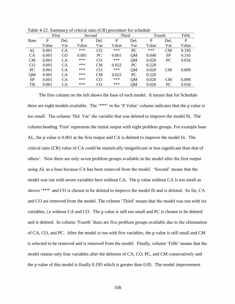
108
Table 4-22. Summary of critical ratio (CR) procedure for schedule
Base
First Second Third Fourth Fifth
P
Value
Del.
Var
P
Value
Del.
Var
P
Value
Del.
Var
P
Value
Del.
Var
P
Value
AL 0.001 CA *** CO *** PC *** CM 0.195
CA 0.001 CO 0.001 PC 0.001 QM 0.040 SP 0.316
CM 0.001 CA *** CO *** QM 0.020 PC 0.034
CO 0.001 CA *** CM 0.022 PC 0.220
PC 0.001 CA *** CO *** QM 0.020 CM 0.899
QM 0.001 CA *** CM 0.022 PC 0.220
SP 0.001 CA *** CO *** QM 0.020 CM 0.899
TB 0.001 CA *** CO *** QM 0.020 PC 0.034
The first column on the left shows the base of each model. It means that for Schedule
there are eight models available. The „***‟ in the „P Value‟ column indicates that the p value is
too small. The column „Del. Var‟ the variable that was deleted to improve the model fit. The
column heading „First‟ represents the initial output with eight problem groups. For example base
AL, the p value is 0.001 at the first output and CA is deleted to improve the model fit. The
critical ratio (CR) value of CA could be statistically insignificant or less significant than that of
others‟. Now there are only seven problem groups available in the model after the first output
using AL as a base because CA has been removed from the model. „Second‟ means that the
model was run with seven variables here without CA. The p value without CA is too small as
shown „***‟ and CO is chosen to be deleted to improve the model fit and is deleted. So far, CA
and CO are removed from the model. The column „Third‟ means that the model was run with six
variables, i.e without CA and CO. The p value is still too small and PC is chosen to be deleted
and is deleted. In column „Fourth‟ there are five problem groups available due to the elimination
of CA, CO, and PC. After the model is run with five variables, the p value is still small and CM
is selected to be removed and is removed from the model. Finally, column „Fifth‟ means that the
model retains only four variables after the deletion of CA, CO, PC, and CM consecutively and
the p value of this model is finally 0.195 which is greater than 0.05. The model improvement
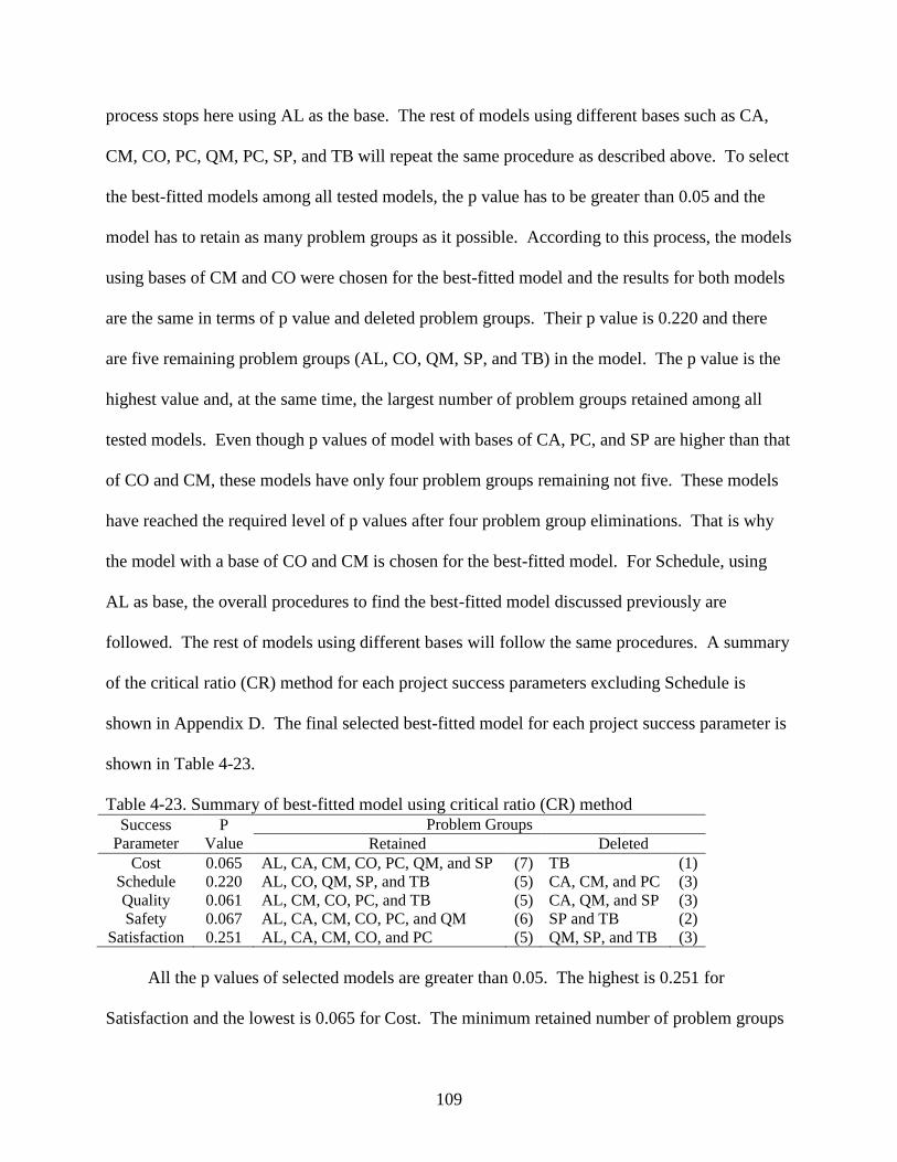
109
process stops here using AL as the base. The rest of models using different bases such as CA,
CM, CO, PC, QM, PC, SP, and TB will repeat the same procedure as described above. To select
the best-fitted models among all tested models, the p value has to be greater than 0.05 and the
model has to retain as many problem groups as it possible. According to this process, the models
using bases of CM and CO were chosen for the best-fitted model and the results for both models
are the same in terms of p value and deleted problem groups. Their p value is 0.220 and there
are five remaining problem groups (AL, CO, QM, SP, and TB) in the model. The p value is the
highest value and, at the same time, the largest number of problem groups retained among all
tested models. Even though p values of model with bases of CA, PC, and SP are higher than that
of CO and CM, these models have only four problem groups remaining not five. These models
have reached the required level of p values after four problem group eliminations. That is why
the model with a base of CO and CM is chosen for the best-fitted model. For Schedule, using
AL as base, the overall procedures to find the best-fitted model discussed previously are
followed. The rest of models using different bases will follow the same procedures. A summary
of the critical ratio (CR) method for each project success parameters excluding Schedule is
shown in Appendix D. The final selected best-fitted model for each project success parameter is
shown in Table 4-23.
Table 4-23. Summary of best-fitted model using critical ratio (CR) method
Success
Parameter
P
Value
Problem Groups
Retained Deleted
Cost 0.065 AL, CA, CM, CO, PC, QM, and SP (7) TB (1)
Schedule 0.220 AL, CO, QM, SP, and TB (5) CA, CM, and PC (3)
Quality 0.061 AL, CM, CO, PC, and TB (5) CA, QM, and SP (3)
Safety 0.067 AL, CA, CM, CO, PC, and QM (6) SP and TB (2)
Satisfaction 0.251 AL, CA, CM, CO, and PC (5) QM, SP, and TB (3)
All the p values of selected models are greater than 0.05. The highest is 0.251 for
Satisfaction and the lowest is 0.065 for Cost. The minimum retained number of problem groups
110
is five for Schedule, Quality, and Satisfaction. The maximum retained number of problem
groups is seven for Cost. Safety has six remaining problem groups in the model. According to
the critical ratio (CR) method, each success parameter is manifested by the remaining problem
groups. The deleted problem groups may affect the model fitting of the original eight-problem
group model. The critical ratio (CR) method was originally intended to delete a path that is not
significant but has been revised to delete a problem group that is not significant or less
significant than others. With respect to this revision, it does not seem that it is a good index to
find the best-fitted model. One of the reasons is that most of time the p value does not improve
whenever a problem group is removed from the model. There is a significant improvement after
three or more problem groups have been deleted. Before that point, it is hard to notice the
improvement of model. The revision of the concept of critical ratio (CR) method may not apply
effectively to this process. It may be necessary to check all possible combinations of problem
groups for the best-fitted model of each success parameter with different numbers of problem
groups.
All possible combination of problem groups method
There are originally eight problem groups per project success parameter. If each CFA
model for success parameter has seven problem groups, all possible combination of seven or less
problem groups will be computed using Equation 4-1 (Weisstein 2009a) below.
(Equation 4-1)
The total number of sets is n and the number of possible combination is k out of n. If each
model has seven problem groups then the total number of combination will be 8 (8!/[7!(8-7)!])
for each success parameter. On the other hand, if any CFA model has six problem groups, then
the total number of possible combination will be 28 (8!/[6!(8-6)!]). The total number of
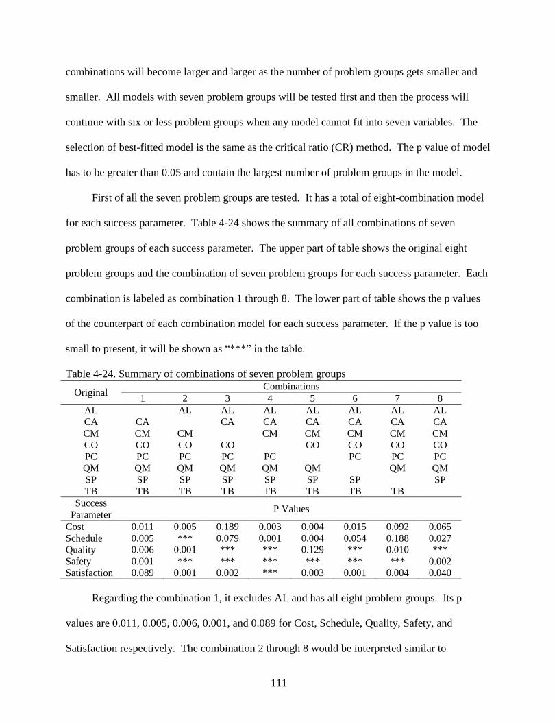
111
combinations will become larger and larger as the number of problem groups gets smaller and
smaller. All models with seven problem groups will be tested first and then the process will
continue with six or less problem groups when any model cannot fit into seven variables. The
selection of best-fitted model is the same as the critical ratio (CR) method. The p value of model
has to be greater than 0.05 and contain the largest number of problem groups in the model.
First of all the seven problem groups are tested. It has a total of eight-combination model
for each success parameter. Table 4-24 shows the summary of all combinations of seven
problem groups of each success parameter. The upper part of table shows the original eight
problem groups and the combination of seven problem groups for each success parameter. Each
combination is labeled as combination 1 through 8. The lower part of table shows the p values
of the counterpart of each combination model for each success parameter. If the p value is too
small to present, it will be shown as “***” in the table.
Table 4-24. Summary of combinations of seven problem groups
Original Combinations
1 2 3 4 5 6 7 8
AL AL AL AL AL AL AL AL
CA CA CA CA CA CA CA CA
CM CM CM CM CM CM CM CM
CO CO CO CO CO CO CO CO
PC PC PC PC PC PC PC PC
QM QM QM QM QM QM QM QM
SP SP SP SP SP SP SP SP
TB TB TB TB TB TB TB TB
Success
Parameter P Values
Cost 0.011 0.005 0.189 0.003 0.004 0.015 0.092 0.065
Schedule 0.005 *** 0.079 0.001 0.004 0.054 0.188 0.027
Quality 0.006 0.001 *** *** 0.129 *** 0.010 ***
Safety 0.001 *** *** *** *** *** *** 0.002
Satisfaction 0.089 0.001 0.002 *** 0.003 0.001 0.004 0.040
Regarding the combination 1, it excludes AL and has all eight problem groups. Its p
values are 0.011, 0.005, 0.006, 0.001, and 0.089 for Cost, Schedule, Quality, Safety, and
Satisfaction respectively. The combination 2 through 8 would be interpreted similar to
112
combination 1. The highest p value of each success parameter is 0.189, 0.188, 0.129, 0.002, and
0.089 for Cost, Schedule, Quality, Safety, and Satisfaction respectively. Only the p value of
Safety is less than 0.05 and others satisfy the minimum of 0.05. The best-fitted model for Cost
would be the combination 3 with the p value of 0.189 that is the highest even though the p value
of combination 7 and 8 is greater than 0.05. The best-fitted model for Schedule would be the
combination 7. The p values of combinations 3 and 6 are greater than 0.05 but less than that of
combination 7. Quality has the only one combination that has the p value greater than 0.05 so
combination 5 is the best-fitted model for Quality. The best-fitted model for Satisfaction is the
combination 1 with the p value of 0.089 that is the only one p value greater than 0.05.
Unfortunately there is no best-fitted model for Safety, using the seven problems in combination.
It is evident that Safety has to look at six-problem groups combination to find the best-fitted
model. So far there are seven problem groups per model available for Cost, Schedule, Quality,
and Satisfaction using the combination method.
The best-fitted model is found for Cost, Schedule, Quality, and Satisfaction using seven-
problem groups combination. There is no best-fitted model using seven-problem groups
combination for Safety and so it is necessary to find a six problem groups combination for Safety
if possible. A total number of possible six-problem groups combinations is 28 as indicated
earlier. The results of 28 combinations for Safety are shown in Table 4-25. Each row shows a
combination with its p value. The p value will be “***” if it is too small to be presented.
The combination 22 has the highest p value among 28 combination models. This model
does not include AL and TB. The second highest is 0.130 from the combination 16 without CA
and TB. So the best-fitted model for Safety is the combination 22 with the problem groups of
CA, CM, CO, PC, QM, and SP. Using all possible combination methods, the best-fitted model
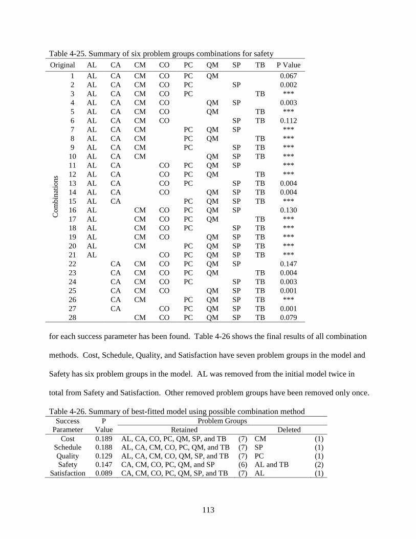
113
Table 4-25. Summary of six problem groups combinations for safety
Original AL CA CM CO PC QM SP TB P Value
Com
bin
atio
ns
1 AL CA CM CO PC QM 0.067
2 AL CA CM CO PC SP 0.002
3 AL CA CM CO PC TB ***
4 AL CA CM CO QM SP 0.003
5 AL CA CM CO QM TB ***
6 AL CA CM CO SP TB 0.112
7 AL CA CM PC QM SP *** 8 AL CA CM PC QM TB *** 9 AL CA CM PC SP TB *** 10 AL CA CM QM SP TB *** 11 AL CA CO PC QM SP *** 12 AL CA CO PC QM TB *** 13 AL CA CO PC SP TB 0.004
14 AL CA CO QM SP TB 0.004
15 AL CA PC QM SP TB ***
16 AL CM CO PC QM SP 0.130
17 AL CM CO PC QM TB *** 18 AL CM CO PC SP TB *** 19 AL CM CO QM SP TB *** 20 AL CM PC QM SP TB *** 21 AL CO PC QM SP TB *** 22 CA CM CO PC QM SP 0.147
23 CA CM CO PC QM TB 0.004
24 CA CM CO PC SP TB 0.003
25 CA CM CO QM SP TB 0.001
26 CA CM PC QM SP TB ***
27 CA CO PC QM SP TB 0.001
28 CM CO PC QM SP TB 0.079
for each success parameter has been found. Table 4-26 shows the final results of all combination
methods. Cost, Schedule, Quality, and Satisfaction have seven problem groups in the model and
Safety has six problem groups in the model. AL was removed from the initial model twice in
total from Safety and Satisfaction. Other removed problem groups have been removed only once.
Table 4-26. Summary of best-fitted model using possible combination method
Success
Parameter
P
Value
Problem Groups
Retained Deleted
Cost 0.189 AL, CA, CO, PC, QM, SP, and TB (7) CM (1)
Schedule 0.188 AL, CA, CM, CO, PC, QM, and TB (7) SP (1)
Quality 0.129 AL, CA, CM, CO, QM, SP, and TB (7) PC (1)
Safety 0.147 CA, CM, CO, PC, QM, and SP (6) AL and TB (2)
Satisfaction 0.089 CA, CM, CO, PC, QM, SP, and TB (7) AL (1)
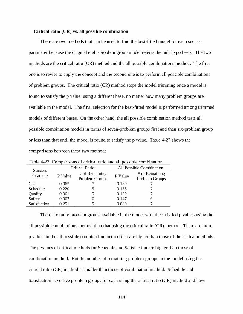
114
Critical ratio (CR) vs. all possible combination
There are two methods that can be used to find the best-fitted model for each success
parameter because the original eight-problem group model rejects the null hypothesis. The two
methods are the critical ratio (CR) method and the all possible combinations method. The first
one is to revise to apply the concept and the second one is to perform all possible combinations
of problem groups. The critical ratio (CR) method stops the model trimming once a model is
found to satisfy the p value, using a different base, no matter how many problem groups are
available in the model. The final selection for the best-fitted model is performed among trimmed
models of different bases. On the other hand, the all possible combination method tests all
possible combination models in terms of seven-problem groups first and then six-problem group
or less than that until the model is found to satisfy the p value. Table 4-27 shows the
comparisons between these two methods.
Table 4-27. Comparisons of critical ratio and all possible combination
Success
Parameter
Critical Ratio All Possible Combination
P Value # of Remaining
Problem Groups P Value
# of Remaining
Problem Groups
Cost 0.065 7 0.189 7
Schedule 0.220 5 0.188 7
Quality 0.061 5 0.129 7
Safety 0.067 6 0.147 6
Satisfaction 0.251 5 0.089 7
There are more problem groups available in the model with the satisfied p values using the
all possible combinations method than that using the critical ratio (CR) method. There are more
p values in the all possible combination method that are higher than those of the critical methods.
The p values of critical methods for Schedule and Satisfaction are higher than those of
combination method. But the number of remaining problem groups in the model using the
critical ratio (CR) method is smaller than those of combination method. Schedule and
Satisfaction have five problem groups for each using the critical ratio (CR) method and have
115
seven problem groups for each using the all combination method. Although the total number of
tested models using the all combination method would be larger than those for the critical ratio
(CR) method where there are less problem group combinations per model, it clearly shows that
all combination is preferred to find the best-fitted model with a higher number of problem groups
in the model. The revised concept of critical ratio (CR) method may not work effectively in this
model trimming process.
To finalize the model for each success parameter, the selection priority will go to the
highest p value with the largest number of problem groups in the model. There is no issue on
selection of best-fitted model for Cost, Quality, and Safety. All combination models satisfy the
highest p value and the largest number of problem groups. So three models from all combination
method will be chosen as the best-fitted model for Cost, Quality, and Safety. On the other hand,
there may be some issues with Schedule and Satisfaction. The p values of both success
parameters of the critical ratio (CR) method are higher than those of all combination method but
fewer number of problem groups than those of all combination. Which model has to be chosen?
Recalling why all this modeling process is needed for the first time. The initial original eight-
problem group model has rejected the null hypothesis. If any project success parameter is not
manifested by the eight problem groups, then how many possible problem groups can manifest
the project success parameter? If there is any model that meets the minimum p value with a
larger number of problem groups, then that model will have to be selected for the best-fitted
model. So the model of Schedule and Satisfaction from the all combinations method has to be
chosen to be the best-fitted model. If the all combinations method had been performed first for
Schedule and Satisfaction, the model trimming process using the critical ratio (CR) method
would not have been necessary because there is a model that meets the p value with seven
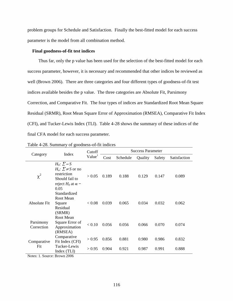
116
problem groups for Schedule and Satisfaction. Finally the best-fitted model for each success
parameter is the model from all combination method.
Final goodness-of-fit test indices
Thus far, only the p value has been used for the selection of the best-fitted model for each
success parameter, however, it is necessary and recommended that other indices be reviewed as
well (Brown 2006). There are three categories and four different types of goodness-of-fit test
indices available besides the p value. The three categories are Absolute Fit, Parsimony
Correction, and Comparative Fit. The four types of indices are Standardized Root Mean Square
Residual (SRMR), Root Mean Square Error of Approximation (RMSEA), Comparative Fit Index
(CFI), and Tucker-Lewis Index (TLI). Table 4-28 shows the summary of these indices of the
final CFA model for each success parameter.
Table 4-28. Summary of goodness-of-fit indices
Category Index Cutoff
Value1
Success Parameter
Cost Schedule Quality Safety Satisfaction
2
H0: S
Ha: S or no
restriction
Should fail to
reject H0 at
0.05
> 0.05 0.189 0.188 0.129 0.147 0.089
Absolute Fit
Standardized
Root Mean
Square
Residual
(SRMR)
< 0.08 0.039 0.065 0.034 0.032 0.062
Parsimony
Correction
Root Mean
Square Error of
Approximation
(RMSEA)
< 0.10 0.056 0.056 0.066 0.070 0.074
Comparative
Fit
Comparative
Fit Index (CFI) > 0.95 0.856 0.881 0.980 0.986 0.832
Tucker-Lewis
Index (TLI) > 0.95 0.904 0.921 0.987 0.991 0.888
Notes: 1. Source: Brown 2006
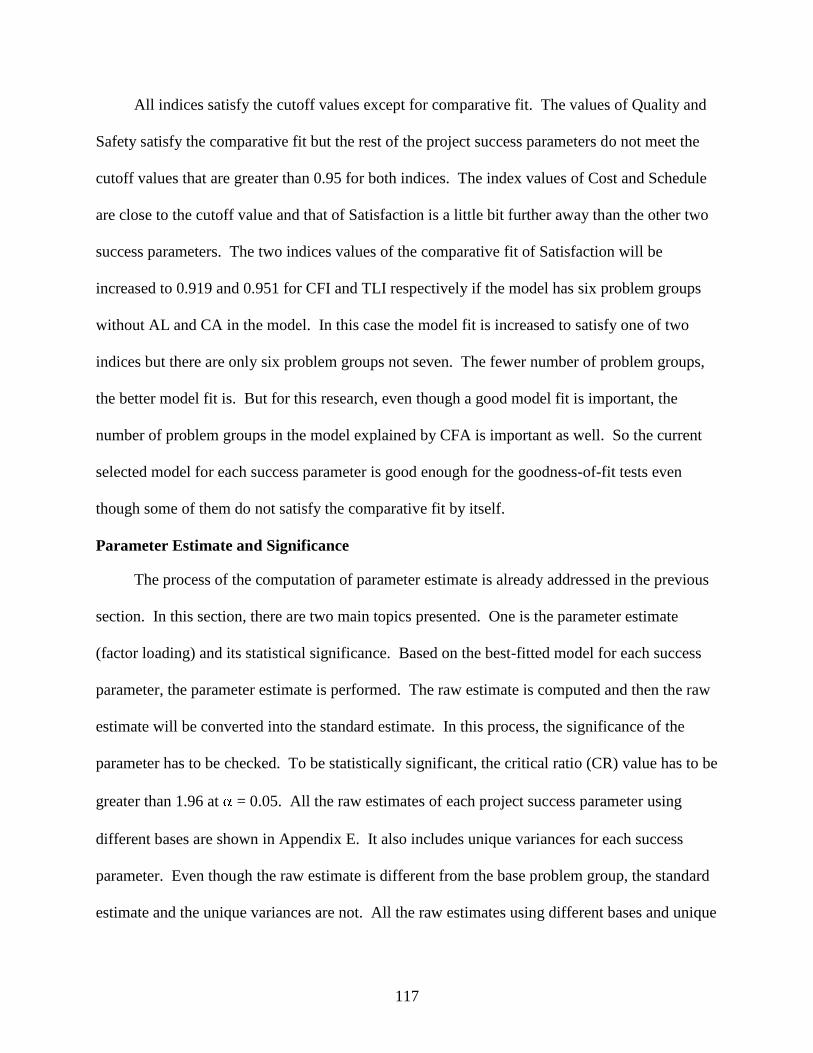
117
All indices satisfy the cutoff values except for comparative fit. The values of Quality and
Safety satisfy the comparative fit but the rest of the project success parameters do not meet the
cutoff values that are greater than 0.95 for both indices. The index values of Cost and Schedule
are close to the cutoff value and that of Satisfaction is a little bit further away than the other two
success parameters. The two indices values of the comparative fit of Satisfaction will be
increased to 0.919 and 0.951 for CFI and TLI respectively if the model has six problem groups
without AL and CA in the model. In this case the model fit is increased to satisfy one of two
indices but there are only six problem groups not seven. The fewer number of problem groups,
the better model fit is. But for this research, even though a good model fit is important, the
number of problem groups in the model explained by CFA is important as well. So the current
selected model for each success parameter is good enough for the goodness-of-fit tests even
though some of them do not satisfy the comparative fit by itself.
Parameter Estimate and Significance
The process of the computation of parameter estimate is already addressed in the previous
section. In this section, there are two main topics presented. One is the parameter estimate
(factor loading) and its statistical significance. Based on the best-fitted model for each success
parameter, the parameter estimate is performed. The raw estimate is computed and then the raw
estimate will be converted into the standard estimate. In this process, the significance of the
parameter has to be checked. To be statistically significant, the critical ratio (CR) value has to be
greater than 1.96 at = 0.05. All the raw estimates of each project success parameter using
different bases are shown in Appendix E. It also includes unique variances for each success
parameter. Even though the raw estimate is different from the base problem group, the standard
estimate and the unique variances are not. All the raw estimates using different bases and unique
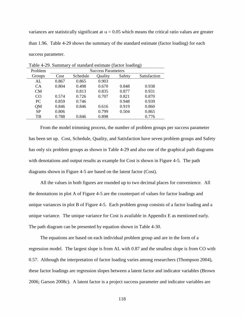
118
variances are statistically significant at = 0.05 which means the critical ratio values are greater
than 1.96. Table 4-29 shows the summary of the standard estimate (factor loading) for each
success parameter.
Table 4-29. Summary of standard estimate (factor loading)
Problem
Groups
Success Parameters
Cost Schedule Quality Safety Satisfaction
AL 0.867 0.865 0.903
CA 0.804 0.498 0.670 0.848 0.938
CM 0.813 0.835 0.877 0.931
CO 0.574 0.726 0.707 0.821 0.870
PC 0.859 0.746 0.948 0.939
QM 0.846 0.846 0.616 0.919 0.860
SP 0.806 0.799 0.504 0.865
TB 0.788 0.846 0.898 0.776
From the model trimming process, the number of problem groups per success parameter
has been set up. Cost, Schedule, Quality, and Satisfaction have seven problem groups and Safety
has only six problem groups as shown in Table 4-29 and also one of the graphical path diagrams
with denotations and output results as example for Cost is shown in Figure 4-5. The path
diagrams shown in Figure 4-5 are based on the latent factor (Cost).
All the values in both figures are rounded up to two decimal places for convenience. All
the denotations in plot A of Figure 4-5 are the counterpart of values for factor loadings and
unique variances in plot B of Figure 4-5. Each problem group consists of a factor loading and a
unique variance. The unique variance for Cost is available in Appendix E as mentioned early.
The path diagram can be presented by equation shown in Table 4-30.
The equations are based on each individual problem group and are in the form of a
regression model. The largest slope is from AL with 0.87 and the smallest slope is from CO with
0.57. Although the interpretation of factor loading varies among researchers (Thompson 2004),
these factor loadings are regression slopes between a latent factor and indicator variables (Brown
2006; Garson 2008c). A latent factor is a project success parameter and indicator variables are
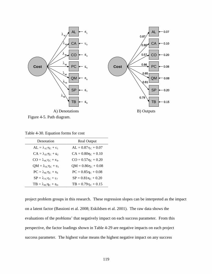
119
Cost
4
1
2
AL
CA
CO
1C
2C
4C
8
7
5
6
PC
QM
SP
TB
8C
5C
6C
7C
Cost
4
1
2
AL
CA
CO
1C
2C
4C
8
7
5
6
PC
QM
SP
TB
8C
5C
6C
7C
Cost
0.20
0.07
0.10
AL
CA
CO
0.87
0.15
0.20
0.08
0.08
PC
QM
SP
TB
0.80
0.57
0.86
0.85
0.81
0.79
Cost
0.20
0.07
0.10
AL
CA
CO
0.87
0.15
0.20
0.08
0.08
PC
QM
SP
TB
0.80
0.57
0.86
0.85
0.81
0.79
A) Denotations B) Outputs
Figure 4-5. Path diagram.
Table 4-30. Equation forms for cost
Denotation Real Output
AL = 1C C + 1 AL = 0.87 C + 0.07
CA = 2C C + 2 CA = 0.80 C + 0.10
CO = 4C C + 4. CO = 0.57 C + 0.20
QM = 5C C + 5 QM = 0.86 C + 0.08
PC = 6C C + 6 PC = 0.85 C + 0.08
SP = 7C C + 7 SP = 0.81 C + 0.20
TB = 8C C + 8. TB = 0.79 C + 0.15
project problem groups in this research. These regression slopes can be interpreted as the impact
on a latent factor (Bassioni et al. 2008; Eskildsen et al. 2001). The raw data shows the
evaluations of the problems‟ that negatively impact on each success parameter. From this
perspective, the factor loadings shown in Table 4-29 are negative impacts on each project
success parameter. The highest value means the highest negative impact on any success
120
parameter and the lowest value means the lowest impact on any success parameter. Most of
problem groups have different impacts on each project success parameter. It supports one of the
hypotheses of this research, that “each problem group will have a different impact on each
success parameter.”
The CFA model procedures for this research have been addressed. The five initial CFA
models, from the 100 point data set, have eight problem groups to be tested whether they are
manifested by all eight problem groups or not. At the end of the process, none of them are
manifested by eight problem groups but it is found that each project success parameter is
manifested by six or seven problem groups. The impacts of problems on each project success
parameter are different from each other. Most of problem groups dynamically and differently
response to each project success parameter. This information on the number of problem groups
within each project success parameter and impacts of the problem groups on success parameters
will be useful and can be a good guideline for further studies on the multiple project success
parameters. The next chapter will be discussed how this information can be used for developing
a tool for potential project problem identification.
121
CHAPTER 5
APPLICATION OF CFA MODEL OUTPUTS
Background
In the preceding chapter, the relationship between certain project success parameters and
some problem groups has been discussed. Each problem group has a different impact on a
project success parameter. It is clear and easy to manage or focus on which problem group has
the most negative impact when there is only one project success parameter. In the reality, there
are more than one project success parameters. The two most common project success
parameters are cost and schedule. A project is considered as successful when it is completed
under budget and within schedule. So there are many articles available on these two project
success parameters such as index modeling (Gibson and Dumont 1995); performance measure
and project outcome forecasting (Choi et al. 2006; Russell et al. 1996). These studies focused on
cost and schedule. As society changes rapidly, the demands on the construction industry are not
focusing on only cost and schedule any more. There are additional success parameters other than
cost and schedule such as quality and safety. Even though Choi et al (2006) addresses multiple
project success parameters and project outcome forecasting, it mainly discusses each individual
success parameter. It does not see the multiple project success parameters as one whole project
success when a project has more than two success parameters with a different weight on each
success parameter. Griffith et al (1999) shows how project success index could be computed and
changed depending upon the criteria and their weights. If there are multiple project success
parameters available with different weight priorities for a project, then how can this project be
controlled? When the project has its own potential problems, which problems should be
considered as the most serious or critical for the project success? Using outputs of the previous
122
chapter and the SMARTS technique, this chapter will show the process involved in coming up
with the answer those questions.
Single Multi-Attribute Rating Technique Using Swing Weight (SMARTS)
Overview
In Chapter 2, the basic procedure of SMARTS has been discussed. This method is helpful
to narrow down the options based on the evaluation of options related to attributes as discussed
in Chapter 2. Attributes would be project success parameters and options would be eight project
problem groups for this research. To use this technique, there are two concerns about the
independence properties of the measurement attributes. One is the value independence and the
other is defined as environmental independence (Edwards 1977; Oyetunji 2001). Another
concern with the values is the dominance among options (Edwards and Barron 1994; Winterfeldt
and Edwards 1986). Any option dominating others should be eliminated. All of the input values
should meet these criteria to use this technique. In this section, the computation of input values,
independence properties, dominance option, and tool development and its validation process will
be discussed.
Computation of Input Values
To perform SMARTS, there needs to be a set of input values for multi-attributes (project
success parameters) and their options (problem groups). In the preceding chapter, the
relationships between project success parameters and eight problem groups is defined as shown
in Table 4-29. The values shown in Table 4-29 consider the impact of each problem group on
each success parameter. The higher the values, the more negative the impact on a project
success parameter. So the values in Table 4-29 are good enough as input values for SMARTS.
The raw values are showing as values with three decimal places so they have to be converted
into whole numbers for the convenience of further work in this process. There are two
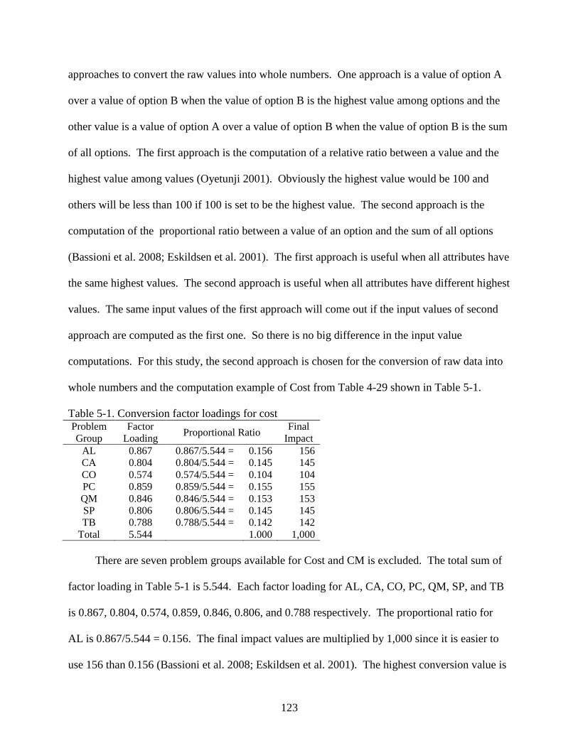
123
approaches to convert the raw values into whole numbers. One approach is a value of option A
over a value of option B when the value of option B is the highest value among options and the
other value is a value of option A over a value of option B when the value of option B is the sum
of all options. The first approach is the computation of a relative ratio between a value and the
highest value among values (Oyetunji 2001). Obviously the highest value would be 100 and
others will be less than 100 if 100 is set to be the highest value. The second approach is the
computation of the proportional ratio between a value of an option and the sum of all options
(Bassioni et al. 2008; Eskildsen et al. 2001). The first approach is useful when all attributes have
the same highest values. The second approach is useful when all attributes have different highest
values. The same input values of the first approach will come out if the input values of second
approach are computed as the first one. So there is no big difference in the input value
computations. For this study, the second approach is chosen for the conversion of raw data into
whole numbers and the computation example of Cost from Table 4-29 shown in Table 5-1.
Table 5-1. Conversion factor loadings for cost Problem
Group
Factor
Loading Proportional Ratio
Final
Impact
AL 0.867 0.867/5.544 = 0.156 156
CA 0.804 0.804/5.544 = 0.145 145
CO 0.574 0.574/5.544 = 0.104 104
PC 0.859 0.859/5.544 = 0.155 155
QM 0.846 0.846/5.544 = 0.153 153
SP 0.806 0.806/5.544 = 0.145 145
TB 0.788 0.788/5.544 = 0.142 142
Total 5.544 1.000 1,000
There are seven problem groups available for Cost and CM is excluded. The total sum of
factor loading in Table 5-1 is 5.544. Each factor loading for AL, CA, CO, PC, QM, SP, and TB
is 0.867, 0.804, 0.574, 0.859, 0.846, 0.806, and 0.788 respectively. The proportional ratio for
AL is 0.867/5.544 = 0.156. The final impact values are multiplied by 1,000 since it is easier to
use 156 than 0.156 (Bassioni et al. 2008; Eskildsen et al. 2001). The highest conversion value is
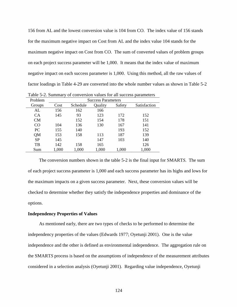
124
156 from AL and the lowest conversion value is 104 from CO. The index value of 156 stands
for the maximum negative impact on Cost from AL and the index value 104 stands for the
maximum negative impact on Cost from CO. The sum of converted values of problem groups
on each project success parameter will be 1,000. It means that the index value of maximum
negative impact on each success parameter is 1,000. Using this method, all the raw values of
factor loadings in Table 4-29 are converted into the whole number values as shown in Table 5-2
Table 5-2. Summary of conversion values for all success parameters
Problem
Groups
Success Parameters
Cost Schedule Quality Safety Satisfaction
AL 156 162 166
CA 145 93 123 172 152
CM 152 154 178 151
CO 104 136 130 167 141
PC 155 140 193 152
QM 153 158 113 187 139
SP 145 147 103 140
TB 142 158 165 126
Sum 1,000 1,000 1,000 1,000 1,000
The conversion numbers shown in the table 5-2 is the final input for SMARTS. The sum
of each project success parameter is 1,000 and each success parameter has its highs and lows for
the maximum impacts on a given success parameter. Next, these conversion values will be
checked to determine whether they satisfy the independence properties and dominance of the
options.
Independency Properties of Values
As mentioned early, there are two types of checks to be performed to determine the
independency properties of the values (Edwards 1977; Oyetunji 2001). One is the value
independence and the other is defined as environmental independence. The aggregation rule on
the SMARTS process is based on the assumptions of independence of the measurement attributes
considered in a selection analysis (Oyetunji 2001). Regarding value independence, Oyetunji
125
(2001) addresses “value independency, which applies essentially to objective measurement
attributes that are assessed in natural units.” As shown in Table 4-29, the values of factor
loadings are showing relationships between success parameters and the problem groups. The
values in Table 4-29 show that there is no relationship between problem groups. Due to the
relationship between success parameters and problem groups, each problem group is naturally
independent from each other. It means that they satisfy the value independency. For the
convenience of the application, all input values are computed into scales out of 1,000. Edwards
(1977) defines the value independence means that the extent of an impact for problem A over B
of a success parameter is unaffected by the position of the entity being evaluated on other
success parameters. The final conversion values satisfy the value independency because all
factor loadings are converted into maximum impact using the proportional ratio on success
parameters. A conversion value is an impact for problem group over the overall impacts. This
meets the definition of the value independency as well.
The other aspect of the independence properties is environmental independence. The
environmental independence indicates the lack of correlation between the levels of problem
groups with respect to two project success parameters (Oyetunji 2001). For example the values
of Cost and Schedule are compared to problem group by problem group. If the ways the values
exist by problem groups are similar, then the correlation between Cost and Schedule will be high.
If the pattern of values by problem groups is the same to both, the correlation will be 1.0. In this
case, a perfect correlation is a violation of the environmental independence and it can lead to
double counting (Edwards 1977). Due to this double counting, if two project parameters are
perfectly environmentally correlated, only one of them need be included in the evaluation
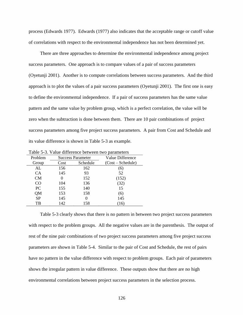
126
process (Edwards 1977). Edwards (1977) also indicates that the acceptable range or cutoff value
of correlations with respect to the environmental independence has not been determined yet.
There are three approaches to determine the environmental independence among project
success parameters. One approach is to compare values of a pair of success parameters
(Oyetunji 2001). Another is to compute correlations between success parameters. And the third
approach is to plot the values of a pair success parameters (Oyetunji 2001). The first one is easy
to define the environmental independence. If a pair of success parameters has the same value
pattern and the same value by problem group, which is a perfect correlation, the value will be
zero when the subtraction is done between them. There are 10 pair combinations of project
success parameters among five project success parameters. A pair from Cost and Schedule and
its value difference is shown in Table 5-3 as example.
Table 5-3. Value difference between two parameters
Problem
Group
Success Parameter Value Difference
(Cost – Schedule) Cost Schedule
AL 156 162 (6)
CA 145 93 52
CM 0 152 (152)
CO 104 136 (32)
PC 155 140 15
QM 153 158 (6)
SP 145 0 145
TB 142 158 (16)
Table 5-3 clearly shows that there is no pattern in between two project success parameters
with respect to the problem groups. All the negative values are in the parenthesis. The output of
rest of the nine pair combinations of two project success parameters among five project success
parameters are shown in Table 5-4. Similar to the pair of Cost and Schedule, the rest of pairs
have no pattern in the value difference with respect to problem groups. Each pair of parameters
shows the irregular pattern in value difference. These outputs show that there are no high
environmental correlations between project success parameters in the selection process.
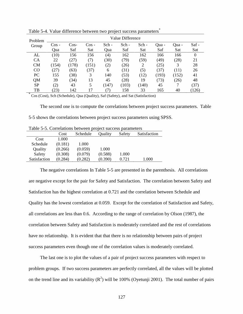
127
Table 5-4. Value difference between two project success parameters*
Problem
Group
Value Difference
Cos - Cos- Cos - Sch - Sch - Sch - Qua - Qua - Saf -
Qua Saf Sat Qua Saf Sat Saf Sat Sat
AL (10) 156 156 (4) 162 162 166 166 0
CA 22 (27) (7) (30) (79) (59) (49) (28) 21
CM (154) (178) (151) (2) (26) 2 (25) 3 28
CO (27) (63) (37) 6 (31) (5) (37) (11) 26
PC 155 (38) 3 140 (53) (12) (193) (152) 41
QM 39 (34) 13 45 (28) 19 (73) (26) 48
SP (2) 43 5 (147) (103) (140) 45 7 (37)
TB (23) 142 17 (7) 158 33 165 40 (126) * Cos (Cost), Sch (Schedule), Qua (Quality), Saf (Safety), and Sat (Satisfaction)
The second one is to compute the correlations between project success parameters. Table
5-5 shows the correlations between project success parameters using SPSS.
Table 5-5. Correlations between project success parameters Cost Schedule Quality Safety Satisfaction
Cost 1.000
Schedule (0.181) 1.000
Quality (0.266) (0.059) 1.000
Safety (0.308) (0.079) (0.588) 1.000
Satisfaction (0.284) (0.282) (0.390) 0.721 1.000
The negative correlations In Table 5-5 are presented in the parenthesis. All correlations
are negative except for the pair for Safety and Satisfaction. The correlation between Safety and
Satisfaction has the highest correlation at 0.721 and the correlation between Schedule and
Quality has the lowest correlation at 0.059. Except for the correlation of Satisfaction and Safety,
all correlations are less than 0.6. According to the range of correlation by Olson (1987), the
correlation between Safety and Satisfaction is moderately correlated and the rest of correlations
have no relationship. It is evident that that there is no relationship between pairs of project
success parameters even though one of the correlation values is moderately correlated.
The last one is to plot the values of a pair of project success parameters with respect to
problem groups. If two success parameters are perfectly correlated, all the values will be plotted
on the trend line and its variability (R2) will be 100% (Oyetunji 2001). The total number of pairs
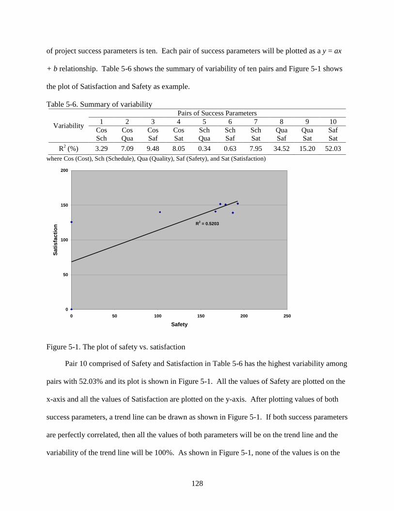
128
of project success parameters is ten. Each pair of success parameters will be plotted as a y = ax
+ b relationship. Table 5-6 shows the summary of variability of ten pairs and Figure 5-1 shows
the plot of Satisfaction and Safety as example.
Table 5-6. Summary of variability
Variability
Pairs of Success Parameters
1 2 3 4 5 6 7 8 9 10
Cos Cos Cos Cos Sch Sch Sch Qua Qua Saf
Sch Qua Saf Sat Qua Saf Sat Saf Sat Sat
R2 (%) 3.29 7.09 9.48 8.05 0.34 0.63 7.95 34.52 15.20 52.03
where Cos (Cost), Sch (Schedule), Qua (Quality), Saf (Safety), and Sat (Satisfaction)
R2 = 0.5203
0
50
100
150
200
0 50 100 150 200 250
Safety
Sa
tis
fac
tio
n
Figure 5-1. The plot of safety vs. satisfaction
Pair 10 comprised of Safety and Satisfaction in Table 5-6 has the highest variability among
pairs with 52.03% and its plot is shown in Figure 5-1. All the values of Safety are plotted on the
x-axis and all the values of Satisfaction are plotted on the y-axis. After plotting values of both
success parameters, a trend line can be drawn as shown in Figure 5-1. If both success parameters
are perfectly correlated, then all the values of both parameters will be on the trend line and the
variability of the trend line will be 100%. As shown in Figure 5-1, none of the values is on the
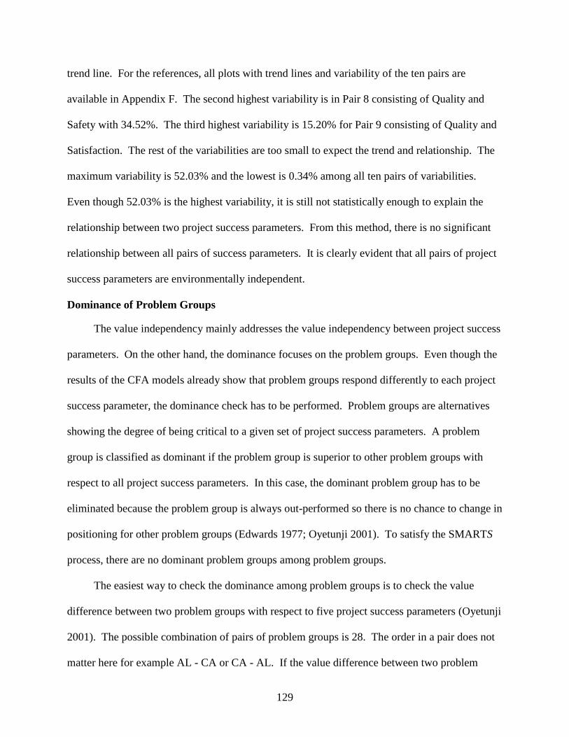
129
trend line. For the references, all plots with trend lines and variability of the ten pairs are
available in Appendix F. The second highest variability is in Pair 8 consisting of Quality and
Safety with 34.52%. The third highest variability is 15.20% for Pair 9 consisting of Quality and
Satisfaction. The rest of the variabilities are too small to expect the trend and relationship. The
maximum variability is 52.03% and the lowest is 0.34% among all ten pairs of variabilities.
Even though 52.03% is the highest variability, it is still not statistically enough to explain the
relationship between two project success parameters. From this method, there is no significant
relationship between all pairs of success parameters. It is clearly evident that all pairs of project
success parameters are environmentally independent.
Dominance of Problem Groups
The value independency mainly addresses the value independency between project success
parameters. On the other hand, the dominance focuses on the problem groups. Even though the
results of the CFA models already show that problem groups respond differently to each project
success parameter, the dominance check has to be performed. Problem groups are alternatives
showing the degree of being critical to a given set of project success parameters. A problem
group is classified as dominant if the problem group is superior to other problem groups with
respect to all project success parameters. In this case, the dominant problem group has to be
eliminated because the problem group is always out-performed so there is no chance to change in
positioning for other problem groups (Edwards 1977; Oyetunji 2001). To satisfy the SMARTS
process, there are no dominant problem groups among problem groups.
The easiest way to check the dominance among problem groups is to check the value
difference between two problem groups with respect to five project success parameters (Oyetunji
2001). The possible combination of pairs of problem groups is 28. The order in a pair does not
matter here for example AL - CA or CA - AL. If the value difference between two problem
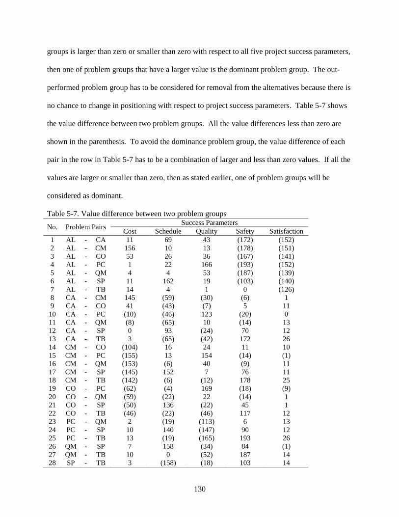
130
groups is larger than zero or smaller than zero with respect to all five project success parameters,
then one of problem groups that have a larger value is the dominant problem group. The out-
performed problem group has to be considered for removal from the alternatives because there is
no chance to change in positioning with respect to project success parameters. Table 5-7 shows
the value difference between two problem groups. All the value differences less than zero are
shown in the parenthesis. To avoid the dominance problem group, the value difference of each
pair in the row in Table 5-7 has to be a combination of larger and less than zero values. If all the
values are larger or smaller than zero, then as stated earlier, one of problem groups will be
considered as dominant.
Table 5-7. Value difference between two problem groups
No. Problem Pairs Success Parameters
Cost Schedule Quality Safety Satisfaction
1 AL - CA 11 69 43 (172) (152)
2 AL - CM 156 10 13 (178) (151)
3 AL - CO 53 26 36 (167) (141)
4 AL - PC 1 22 166 (193) (152)
5 AL - QM 4 4 53 (187) (139)
6 AL - SP 11 162 19 (103) (140)
7 AL - TB 14 4 1 0 (126)
8 CA - CM 145 (59) (30) (6) 1
9 CA - CO 41 (43) (7) 5 11
10 CA - PC (10) (46) 123 (20) 0
11 CA - QM (8) (65) 10 (14) 13
12 CA - SP 0 93 (24) 70 12
13 CA - TB 3 (65) (42) 172 26
14 CM - CO (104) 16 24 11 10
15 CM - PC (155) 13 154 (14) (1)
16 CM - QM (153) (6) 40 (9) 11
17 CM - SP (145) 152 7 76 11
18 CM - TB (142) (6) (12) 178 25
19 CO - PC (62) (4) 169 (18) (9)
20 CO - QM (59) (22) 22 (14) 1
21 CO - SP (50) 136 (22) 45 1
22 CO - TB (46) (22) (46) 117 12
23 PC - QM 2 (19) (113) 6 13
24 PC - SP 10 140 (147) 90 12
25 PC - TB 13 (19) (165) 193 26
26 QM - SP 7 158 (34) 84 (1)
27 QM - TB 10 0 (52) 187 14
28 SP - TB 3 (158) (18) 103 14
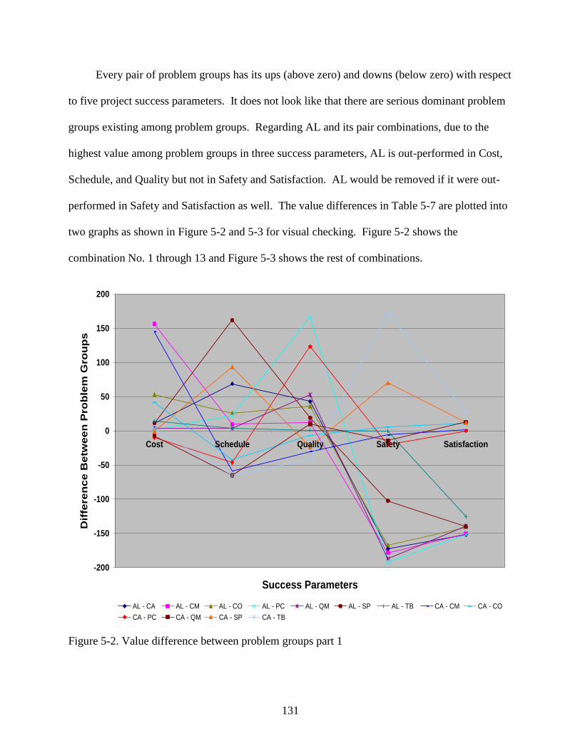
131
Every pair of problem groups has its ups (above zero) and downs (below zero) with respect
to five project success parameters. It does not look like that there are serious dominant problem
groups existing among problem groups. Regarding AL and its pair combinations, due to the
highest value among problem groups in three success parameters, AL is out-performed in Cost,
Schedule, and Quality but not in Safety and Satisfaction. AL would be removed if it were out-
performed in Safety and Satisfaction as well. The value differences in Table 5-7 are plotted into
two graphs as shown in Figure 5-2 and 5-3 for visual checking. Figure 5-2 shows the
combination No. 1 through 13 and Figure 5-3 shows the rest of combinations.
-200
-150
-100
-50
0
50
100
150
200
Cost Schedule Quality Safety Satisfaction
Success Parameters
Dif
fere
nc
e B
etw
ee
n P
rob
lem
Gro
up
s
AL - CA AL - CM AL - CO AL - PC AL - QM AL - SP AL - TB CA - CM CA - CO
CA - PC CA - QM CA - SP CA - TB
Figure 5-2. Value difference between problem groups part 1
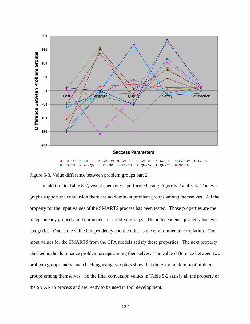
132
-200
-150
-100
-50
0
50
100
150
200
Cost Schedule Quality Safety Satisfaction
Success Parameters
Dif
fere
nce
Be
twe
en
Pro
ble
m G
rou
ps
CM - CO CM - PC CM - QM CM - SP CM - TB CO - PC CO - QM CO - SP
CO - TB PC - QM PC - SP PC - TB QM - SP QM - TB SP - TB
Figure 5-3. Value difference between problem groups part 2
In addition to Table 5-7, visual checking is performed using Figure 5-2 and 5-3. The two
graphs support the conclusion there are no dominant problem groups among themselves. All the
property for the input values of the SMARTS process has been tested. Those properties are the
independency property and dominance of problem groups. The independence property has two
categories. One is the value independency and the other is the environmental correlation. The
input values for the SMARTS from the CFA models satisfy these properties. The next property
checked is the dominance problem groups among themselves. The value difference between two
problem groups and visual checking using two plots show that there are no dominant problem
groups among themselves. So the final conversion values in Table 5-2 satisfy all the property of
the SMARTS process and are ready to be used in tool development.
133
Basic Concept of Application
Overview
As discussed in the section 2.5 of the Chapter 2, the SMARTS process shows the best
alternative (problem group) based on the preferences or weights of factors (project success
parameters) as a form of aggregated scores. The preceding section showed the whole process of
testing the property of input values for the SMARTS process. The input values are the output of
CFA models. Each value in the table is the maximum negative impact of the index value on
each success parameter. The values are various among problem groups and project success
parameters. From this point, there are five project success parameters available with a different
weight or preference and there are eight potential problem groups available with maximum
impact on each success parameter. Using the SMARTS process, the degrees of being critical
problem groups can be computed by changing the weight or preference of project success
parameters. The aggregated scores represent the maximum degree of being critical of a problem
group with respect to the preference or weights of project success parameters. The higher the
aggregated score of a problem group, the most critical problem group is. The SMARTS process
has only one criterion in this study, which is project success parameter. As stated early, all the
values of problem groups are their maximum negative impact on project success parameters. It
would be impossible to have all eight-problem groups as the most critical as they are at the same
time for a project. There will be certainly a difference in the degrees of severity of the problem
groups. So in addition to the project success parameters, it is necessary to add the degree of
severity of the problem group into the application development. The final application has two
criteria, which are five project success parameters and eight project problem groups. In this
section, the process of the computation of aggregated scores using the SMARTS process and the
134
degree of severity of problem group to select the most critical problem group will be showed
using equations and numerical examples for a given scenario.
Scenario
The following is a scenario on the explanation of the SMARTS process and the degree of
severity of the problem for the basic concept of the application. The process will be discussed
based on this scenario and the issues related to this study.
A contractor has been awarded a project. The contractor uses a system that classifies the
problems it encounters on projects into eight (8) problem groups - AL (alignment), CA
(constructability), CM (change management), CO (contracting), PC (project controls), QM
(quality), SP (safety practices), and TB (team building). The severity of problems such as how
serious or minor they are varies among the problem groups. The owner of the project is very
demanding and evaluates their projects based on five different success parameters - cost,
schedule, quality, safety, and satisfaction. The contractor wants to know which problems he has
to be concerned with the most and the least under any given conditions (severity of the problem
and the owner’s priorities based on success parameters) to meet the owner’s expectation on
project.
The issues related to this scenario are:
1) How does the contractor know which of the eight problem groups is the most critical?;
2) How do the problem groups impact each success parameter?;
3) How does the contractor manage the problems to minimize the impacts of problems?;
and
4) How do priority weights of the success parameters affect the impacts of problems?
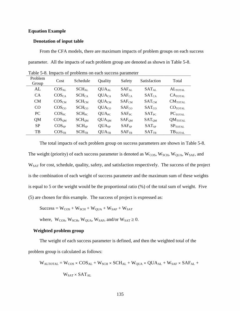
135
Equation Example
Denotation of input table
From the CFA models, there are maximum impacts of problem groups on each success
parameter. All the impacts of each problem group are denoted as shown in Table 5-8.
Table 5-8. Impacts of problems on each success parameter Problem
Group Cost Schedule Quality Safety Satisfaction Total
AL COSAL SCHAL QUAAL SAFAL SATAL ALTOTAL
CA COSCA SCHCA QUACA SAFCA SATCA CATOTAL
CM COSCM SCHCM QUACM SAFCM SATCM CMTOTAL
CO COSCO SCHCO QUACO SAFCO SATCO COTOTAL
PC COSPC SCHPC QUAPC SAFPC SATPC PCTOTAL
QM COSQM SCHQM QUAQM SAFQM SATQM QMTOTAL
SP COSSP SCHSP QUASP SAFSP SATSP SPTOTAL
TB COSTB SCHTB QUATB SAFTB SATTB TBTOTAL
The total impacts of each problem group on success parameters are shown in Table 5-8.
The weight (priority) of each success parameter is denoted as WCOS, WSCH, WQUA, WSAF, and
WSAT for cost, schedule, quality, safety, and satisfaction respectively. The success of the project
is the combination of each weight of success parameter and the maximum sum of these weights
is equal to 5 or the weight would be the proportional ratio (%) of the total sum of weight. Five
(5) are chosen for this example. The success of project is expressed as:
Success = WCOS + WSCH + WQUA + WSAF + WSAT
where, WCOS, WSCH, WQUA, WSAF, and/or WSAT 0.
Weighted problem group
The weight of each success parameter is defined, and then the weighted total of the
problem group is calculated as follows:
WALTOTAL = WCOS COSAL + WSCH SCHAL + WQUA QUAAL + WSAF SAFAL +
WSAT SATAL
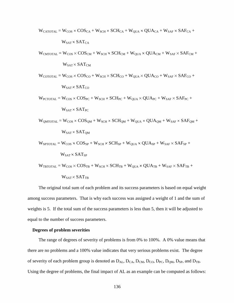
136
WCATOTAL = WCOS COSCA + WSCH SCHCA + WQUA QUACA + WSAF SAFCA +
WSAT SATCA
WCMTOTAL = WCOS COSCM + WSCH SCHCM + WQUA QUACM + WSAF SAFCM +
WSAT SATCM
WCOTOTAL = WCOS COSCO + WSCH SCHCO + WQUA QUACO + WSAF SAFCO +
WSAT SATCO
WPCTOTAL = WCOS COSPC + WSCH SCHPC + WQUA QUAPC + WSAF SAFPC +
WSAT SATPC
WQMTOTAL = WCOS COSQM + WSCH SCHQM + WQUA QUAQM + WSAF SAFQM +
WSAT SATQM
WSPTOTAL = WCOS COSSP + WSCH SCHSP + WQUA QUASP + WSAF SAFSP +
WSAT SATSP
WTBTOTAL = WCOS COSTB + WSCH SCHTB + WQUA QUATB + WSAF SAFTB +
WSAT SATTB
The original total sum of each problem and its success parameters is based on equal weight
among success parameters. That is why each success was assigned a weight of 1 and the sum of
weights is 5. If the total sum of the success parameters is less than 5, then it will be adjusted to
equal to the number of success parameters.
Degrees of problem severities
The range of degrees of severity of problems is from 0% to 100%. A 0% value means that
there are no problems and a 100% value indicates that very serious problems exist. The degree
of severity of each problem group is denoted as DAL, DCA, DCM, DCO, DPC, DQM, DSP, and DTB.
Using the degree of problems, the final impact of AL as an example can be computed as follows:
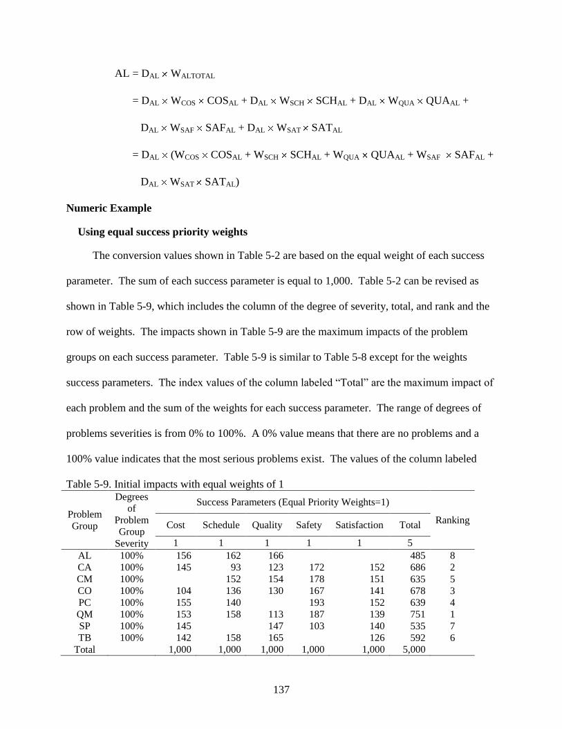
137
AL = DAL WALTOTAL
= DAL WCOS COSAL + DAL WSCH SCHAL + DAL WQUA QUAAL +
DAL WSAF SAFAL + DAL WSAT SATAL
= DAL (WCOS COSAL + WSCH SCHAL + WQUA QUAAL + WSAF SAFAL +
DAL WSAT SATAL)
Numeric Example
Using equal success priority weights
The conversion values shown in Table 5-2 are based on the equal weight of each success
parameter. The sum of each success parameter is equal to 1,000. Table 5-2 can be revised as
shown in Table 5-9, which includes the column of the degree of severity, total, and rank and the
row of weights. The impacts shown in Table 5-9 are the maximum impacts of the problem
groups on each success parameter. Table 5-9 is similar to Table 5-8 except for the weights
success parameters. The index values of the column labeled “Total” are the maximum impact of
each problem and the sum of the weights for each success parameter. The range of degrees of
problems severities is from 0% to 100%. A 0% value means that there are no problems and a
100% value indicates that the most serious problems exist. The values of the column labeled
Table 5-9. Initial impacts with equal weights of 1
Problem
Group
Degrees
of
Problem
Group
Severity
Success Parameters (Equal Priority Weights=1)
Ranking Cost Schedule Quality Safety Satisfaction Total
1 1 1 1 1 5
AL 100% 156 162 166 485 8
CA 100% 145 93 123 172 152 686 2
CM 100% 152 154 178 151 635 5
CO 100% 104 136 130 167 141 678 3
PC 100% 155 140 193 152 639 4
QM 100% 153 158 113 187 139 751 1
SP 100% 145 147 103 140 535 7
TB 100% 142 158 165 126 592 6
Total 1,000 1,000 1,000 1,000 1,000 5,000
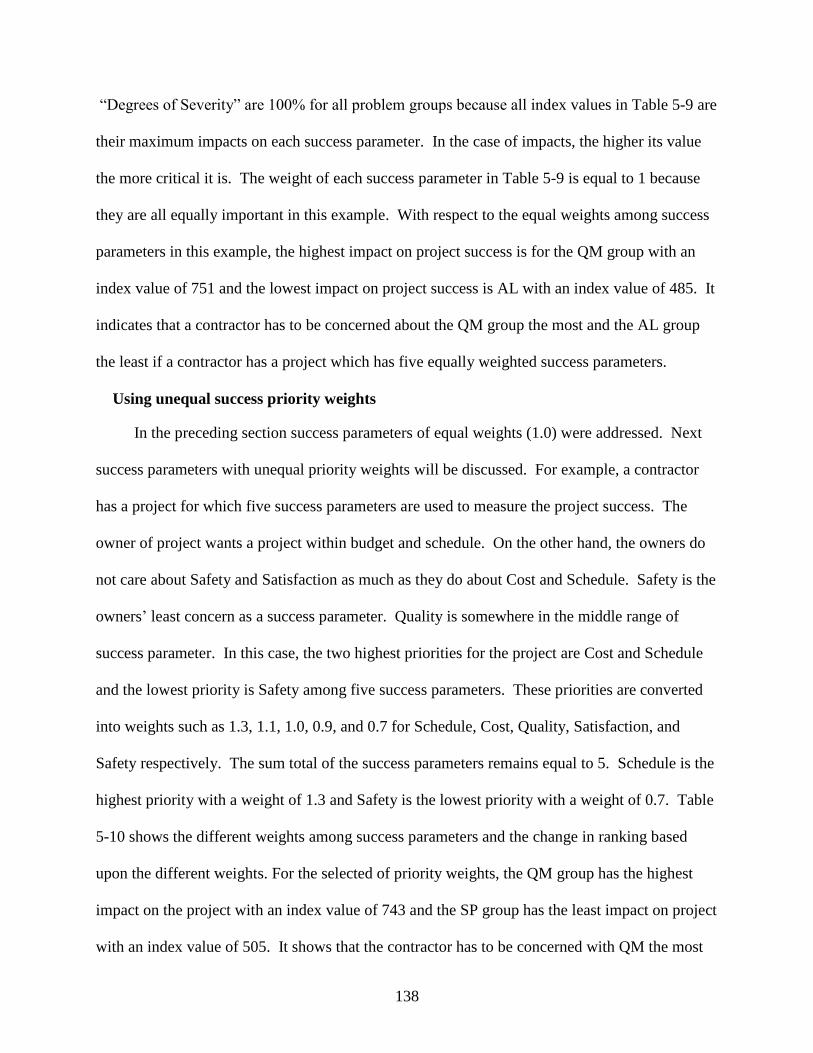
138
“Degrees of Severity” are 100% for all problem groups because all index values in Table 5-9 are
their maximum impacts on each success parameter. In the case of impacts, the higher its value
the more critical it is. The weight of each success parameter in Table 5-9 is equal to 1 because
they are all equally important in this example. With respect to the equal weights among success
parameters in this example, the highest impact on project success is for the QM group with an
index value of 751 and the lowest impact on project success is AL with an index value of 485. It
indicates that a contractor has to be concerned about the QM group the most and the AL group
the least if a contractor has a project which has five equally weighted success parameters.
Using unequal success priority weights
In the preceding section success parameters of equal weights (1.0) were addressed. Next
success parameters with unequal priority weights will be discussed. For example, a contractor
has a project for which five success parameters are used to measure the project success. The
owner of project wants a project within budget and schedule. On the other hand, the owners do
not care about Safety and Satisfaction as much as they do about Cost and Schedule. Safety is the
owners‟ least concern as a success parameter. Quality is somewhere in the middle range of
success parameter. In this case, the two highest priorities for the project are Cost and Schedule
and the lowest priority is Safety among five success parameters. These priorities are converted
into weights such as 1.3, 1.1, 1.0, 0.9, and 0.7 for Schedule, Cost, Quality, Satisfaction, and
Safety respectively. The sum total of the success parameters remains equal to 5. Schedule is the
highest priority with a weight of 1.3 and Safety is the lowest priority with a weight of 0.7. Table
5-10 shows the different weights among success parameters and the change in ranking based
upon the different weights. For the selected of priority weights, the QM group has the highest
impact on the project with an index value of 743 and the SP group has the least impact on project
with an index value of 505. It shows that the contractor has to be concerned with QM the most
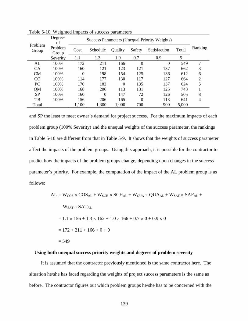
139
Table 5-10. Weighted impacts of success parameters
Problem
Group
Degrees
of
Problem
Group
Severity
Success Parameters (Unequal Priority Weights)
Ranking Cost Schedule Quality Safety Satisfaction Total
1.1 1.3 1.0 0.7 0.9 5
AL 100% 172 211 166 0 0 549 7
CA 100% 160 121 123 121 137 662 3
CM 100% 0 198 154 125 136 612 6
CO 100% 114 177 130 117 127 664 2
PC 100% 170 182 0 135 137 624 5
QM 100% 168 206 113 131 125 743 1
SP 100% 160 0 147 72 126 505 8
TB 100% 156 206 165 0 113 641 4
Total 1,100 1,300 1,000 700 900 5,000
and SP the least to meet owner‟s demand for project success. For the maximum impacts of each
problem group (100% Severity) and the unequal weights of the success parameter, the rankings
in Table 5-10 are different from that in Table 5-9. It shows that the weights of success parameter
affect the impacts of the problem groups. Using this approach, it is possible for the contractor to
predict how the impacts of the problem groups change, depending upon changes in the success
parameter‟s priority. For example, the computation of the impact of the AL problem group is as
follows:
AL = WCOS COSAL + WSCH SCHAL + WQUA QUAAL + WSAF SAFAL +
WSAT SATAL
= 1.1 156 + 1.3 162 + 1.0 166 + 0.7 0 + 0.9 0
= 172 + 211 + 166 + 0 + 0
= 549
Using both unequal success priority weights and degrees of problem severity
It is assumed that the contractor previously mentioned is the same contractor here. The
situation he/she has faced regarding the weights of project success parameters is the same as
before. The contractor figures out which problem groups he/she has to be concerned with the
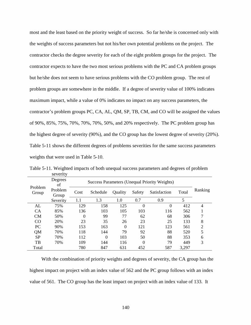
140
most and the least based on the priority weight of success. So far he/she is concerned only with
the weights of success parameters but not his/her own potential problems on the project. The
contractor checks the degree severity for each of the eight problem groups for the project. The
contractor expects to have the two most serious problems with the PC and CA problem groups
but he/she does not seem to have serious problems with the CO problem group. The rest of
problem groups are somewhere in the middle. If a degree of severity value of 100% indicates
maximum impact, while a value of 0% indicates no impact on any success parameters, the
contractor‟s problem groups PC, CA, AL, QM, SP, TB, CM, and CO will be assigned the values
of 90%, 85%, 75%, 70%, 70%, 70%, 50%, and 20% respectively. The PC problem group has
the highest degree of severity (90%), and the CO group has the lowest degree of severity (20%).
Table 5-11 shows the different degrees of problems severities for the same success parameters
weights that were used in Table 5-10.
Table 5-11. Weighted impacts of both unequal success parameters and degrees of problem
severity
Problem
Group
Degrees
of
Problem
Group
Severity
Success Parameters (Unequal Priority Weights)
Ranking Cost Schedule Quality Safety Satisfaction Total
1.1 1.3 1.0 0.7 0.9 5
AL 75% 129 158 125 0 0 412 4
CA 85% 136 103 105 103 116 562 1
CM 50% 0 99 77 62 68 306 7
CO 20% 23 35 26 23 25 133 8
PC 90% 153 163 0 121 123 561 2
QM 70% 118 144 79 92 88 520 5
SP 70% 112 0 103 50 88 353 6
TB 70% 109 144 116 0 79 449 3
Total 780 847 631 452 587 3,297
With the combination of priority weights and degrees of severity, the CA group has the
highest impact on project with an index value of 562 and the PC group follows with an index
value of 561. The CO group has the least impact on project with an index value of 133. It
141
means that the contractor has to monitor the CA and PC groups the most and the CO and CM
groups the least to meet owner‟s demand. The ranking of problems is different from Table 5-9
and 5-10. Table 5-9, 5-10, and 5-11 show how the degrees of problem severities and the weights
assigned to the success parameters affect the final impact of each problem group. The
computation of AL as an example is as follows:
AL = DAL WCOS COSAL + DAL WSCH SCHAL + DAL WQUA QUAAL +
DAL WSAF SAFAL + DAL WSAT SATAL
= 75% 1.1 156 +75% 1.3 162 + 75% 1.0 166 + 75% 0.7 0 +
75% 0.9 0
= 75% 172 + 75% 211 + 75% 166 + 75% 0 + 75% 0
= 129 + 158 + 125 + 0 + 0
= 412
Summary
Changes in impacts of problem groups on a project have been discussed so far. During this
process, it is possible for the contractor to predict what problem groups will be critical for project
success based on the owner‟s success priority and his/her degree of problems severity. As shown
in Table 5-11 using the approach described above the contractor will be able to determine which
problem has the most and the least impact on the project success parameters based on the current
degree of problems severities and success priority weights. The contractor may utilize the
degrees of problems to minimize the impacts on a certain success parameter. If there is a change
in the priorities of success parameters during construction, the contractor will be able to
determine which problem group he/she has to be more concerned with. Table 5-11 is useful to
help both owners and contractors focus on certain potential problem groups in order to satisfy the
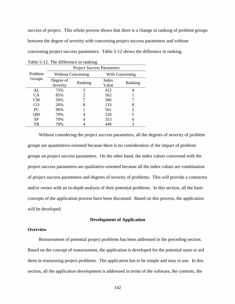
142
success of project. This whole process shows that there is a change in ranking of problem groups
between the degree of severity with concerning project success parameters and without
concerning project success parameters. Table 5-12 shows the difference in ranking.
Table 5-12. The difference in ranking
Problem
Groups
Project Success Parameters
Without Concerning With Concerning
Degree of
Severity Ranking
Index
Value Ranking
AL 75% 3 412 4
CA 85% 2 562 1
CM 50% 7 306 7
CO 20% 8 133 8
PC 90% 1 561 2
QM 70% 4 520 5
SP 70% 4 353 6
TB 70% 4 449 3
Without considering the project success parameters, all the degrees of severity of problem
groups are quantitative-oriented because there is no consideration of the impact of problem
groups on project success parameters. On the other hand, the index values concerned with the
project success parameters are qualitative-oriented because all the index values are combination
of project success parameters and degrees of severity of problems. This will provide a contractor
and/or owner with an in-depth analysis of their potential problems. In this section, all the basic
concepts of the application process have been discussed. Based on this process, the application
will be developed.
Development of Application
Overview
Reassessment of potential project problems has been addressed in the preceding section.
Based on the concept of reassessment, the application is developed for the potential users to aid
them in reassessing project problems. The application has to be simple and easy to use. In this
section, all the application development is addressed in terms of the software, the contents, the
143
difference between the basic concepts explained and the application, and finally the validation of
application.
Application Software Program
The objective of application development is to have an easy and simple to use software
package for the potential users. To keep the application accessible to the largest number of users,
it was developed using Microsoft Office Excel 2003.
Application Description
This application is named the Potential Project Problem Identification Tool because the
final output shows the degrees of being critical of problem groups based on project success
parameters and problems. The tool is available as shown in Object 5-1 below.
Object 5-1. Potential problem identification tool as a Microsoft Excel file (.xls 41kb)
There are four worksheets available in the application file. They are Instruction, Input,
Output, Success Parameters, and Problem Group. The Instruction worksheet gives the users
general information about the application, the Input worksheet is used to assess the project
success parameters and the degrees of severity of problem groups. The output shows a
histogram chart as the final results based on the input. The worksheet of Success Parameters and
Problem Groups addresses the definition of success parameters and problem groups. In the
Instruction worksheet, there are three main subtitles available. The three subtitles are Overview,
Project Success Parameters, and Project Problem Severity. In Overview, the overall purposes
and the basic concepts of this application are addressed. What the outputs mean addresses as
well. In Project Success Parameters worksheet, the instruction of weighing project success
parameters is explained with an example. It will be explained more detailed later. Finally, the
instruction for the degrees of severity of problem groups is explained with an example in Project
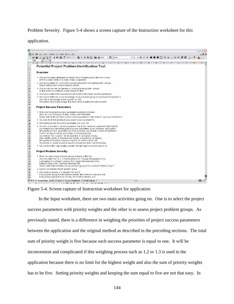
144
Problem Severity. Figure 5-4 shows a screen capture of the Instruction worksheet for this
application.
Figure 5-4. Screen capture of Instruction worksheet for application
In the Input worksheet, there are two main activities going on. One is to select the project
success parameters with priority weights and the other is to assess project problem groups. As
previously stated, there is a difference in weighing the priorities of project success parameters
between the application and the original method as described in the preceding sections. The total
sum of priority weight is five because each success parameter is equal to one. It will be
inconvenient and complicated if this weighing process such as 1.2 or 1.3 is used in the
application because there is no limit for the highest weight and also the sum of priority weights
has to be five. Setting priority weights and keeping the sum equal to five are not that easy. In
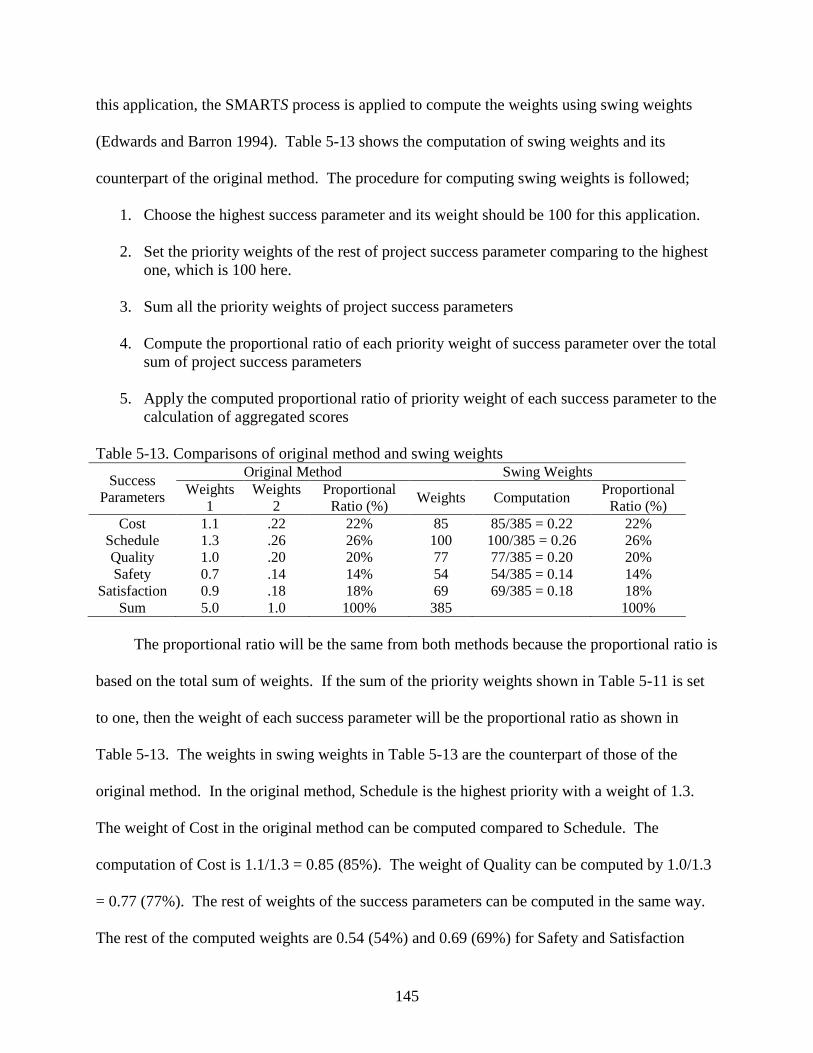
145
this application, the SMARTS process is applied to compute the weights using swing weights
(Edwards and Barron 1994). Table 5-13 shows the computation of swing weights and its
counterpart of the original method. The procedure for computing swing weights is followed;
1. Choose the highest success parameter and its weight should be 100 for this application.
2. Set the priority weights of the rest of project success parameter comparing to the highest
one, which is 100 here.
3. Sum all the priority weights of project success parameters
4. Compute the proportional ratio of each priority weight of success parameter over the total
sum of project success parameters
5. Apply the computed proportional ratio of priority weight of each success parameter to the
calculation of aggregated scores
Table 5-13. Comparisons of original method and swing weights
Success
Parameters
Original Method Swing Weights
Weights
1
Weights
2
Proportional
Ratio (%) Weights Computation
Proportional
Ratio (%)
Cost 1.1 .22 22% 85 85/385 = 0.22 22%
Schedule 1.3 .26 26% 100 100/385 = 0.26 26%
Quality 1.0 .20 20% 77 77/385 = 0.20 20%
Safety 0.7 .14 14% 54 54/385 = 0.14 14%
Satisfaction 0.9 .18 18% 69 69/385 = 0.18 18%
Sum 5.0 1.0 100% 385 100%
The proportional ratio will be the same from both methods because the proportional ratio is
based on the total sum of weights. If the sum of the priority weights shown in Table 5-11 is set
to one, then the weight of each success parameter will be the proportional ratio as shown in
Table 5-13. The weights in swing weights in Table 5-13 are the counterpart of those of the
original method. In the original method, Schedule is the highest priority with a weight of 1.3.
The weight of Cost in the original method can be computed compared to Schedule. The
computation of Cost is 1.1/1.3 = 0.85 (85%). The weight of Quality can be computed by 1.0/1.3
= 0.77 (77%). The rest of weights of the success parameters can be computed in the same way.
The rest of the computed weights are 0.54 (54%) and 0.69 (69%) for Safety and Satisfaction
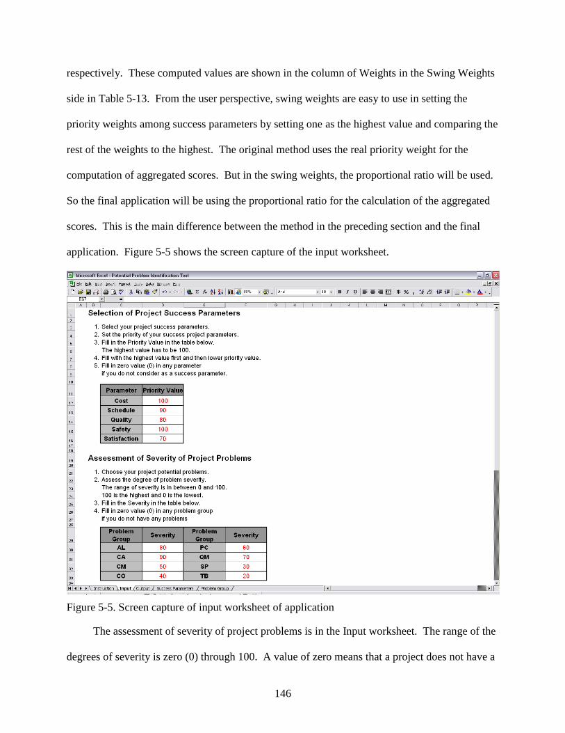
146
respectively. These computed values are shown in the column of Weights in the Swing Weights
side in Table 5-13. From the user perspective, swing weights are easy to use in setting the
priority weights among success parameters by setting one as the highest value and comparing the
rest of the weights to the highest. The original method uses the real priority weight for the
computation of aggregated scores. But in the swing weights, the proportional ratio will be used.
So the final application will be using the proportional ratio for the calculation of the aggregated
scores. This is the main difference between the method in the preceding section and the final
application. Figure 5-5 shows the screen capture of the input worksheet.
Figure 5-5. Screen capture of input worksheet of application
The assessment of severity of project problems is in the Input worksheet. The range of the
degrees of severity is zero (0) through 100. A value of zero means that a project does not have a
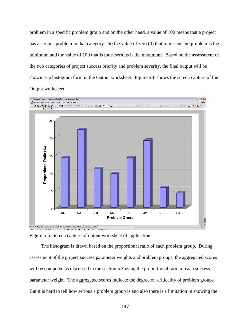
147
problem in a specific problem group and on the other hand, a value of 100 means that a project
has a serious problem in that category. So the value of zero (0) that represents no problem is the
minimum and the value of 100 that is most serious is the maximum. Based on the assessment of
the two categories of project success priority and problem severity, the final output will be
shown as a histogram form in the Output worksheet. Figure 5-6 shows the screen capture of the
Output worksheet.
Figure 5-6. Screen capture of output worksheet of application
The histogram is drawn based on the proportional ratio of each problem group. During
assessment of the project success parameter weights and problem groups, the aggregated scores
will be computed as discussed in the section 5.3 using the proportional ratio of each success
parameter weight. The aggregated scores indicate the degree of criticality of problem groups.
But it is hard to tell how serious a problem group is and also there is a limitation in showing the
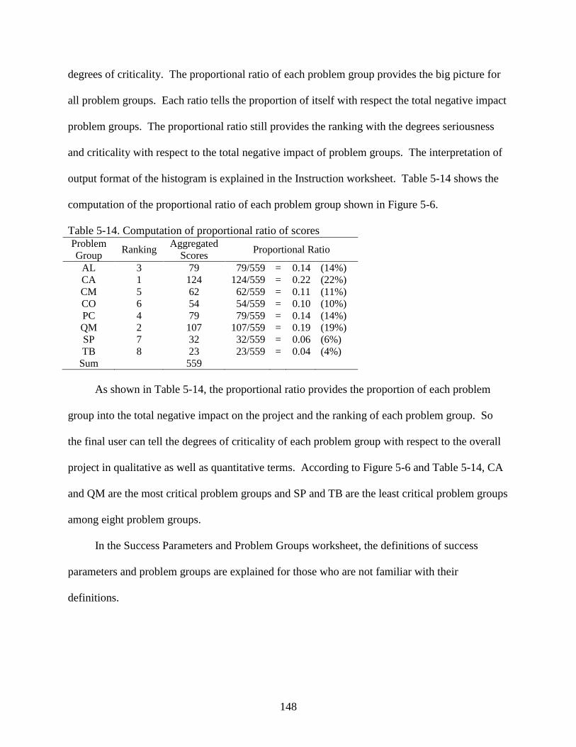
148
degrees of criticality. The proportional ratio of each problem group provides the big picture for
all problem groups. Each ratio tells the proportion of itself with respect the total negative impact
problem groups. The proportional ratio still provides the ranking with the degrees seriousness
and criticality with respect to the total negative impact of problem groups. The interpretation of
output format of the histogram is explained in the Instruction worksheet. Table 5-14 shows the
computation of the proportional ratio of each problem group shown in Figure 5-6.
Table 5-14. Computation of proportional ratio of scores Problem
Group Ranking
Aggregated
Scores Proportional Ratio
AL 3 79 79/559 = 0.14 (14%)
CA 1 124 124/559 = 0.22 (22%)
CM 5 62 62/559 = 0.11 (11%)
CO 6 54 54/559 = 0.10 (10%)
PC 4 79 79/559 = 0.14 (14%)
QM 2 107 107/559 = 0.19 (19%)
SP 7 32 32/559 = 0.06 (6%)
TB 8 23 23/559 = 0.04 (4%)
Sum 559
As shown in Table 5-14, the proportional ratio provides the proportion of each problem
group into the total negative impact on the project and the ranking of each problem group. So
the final user can tell the degrees of criticality of each problem group with respect to the overall
project in qualitative as well as quantitative terms. According to Figure 5-6 and Table 5-14, CA
and QM are the most critical problem groups and SP and TB are the least critical problem groups
among eight problem groups.
In the Success Parameters and Problem Groups worksheet, the definitions of success
parameters and problem groups are explained for those who are not familiar with their
definitions.
149
Validation of Application
Overview
The potential problem identification tool is a decision-making aid, designed for use by
project participants especially project managers and owners in the early phase of projects. Under
given circumstances – priority weights of success parameters and expected problems severity,
this tool will provide project participants with a deep insight of potential project problems. So it
is necessary to validate this tool as a useful guideline for participants. The main output of this
tool is to show the possible future problems based on the combination of priority weights of
success parameters and problem severity. To validate this tool, the comparison of the output of
tool of project problems and actual project problem cases is necessary. If the output of tool is
close to the actual project case, then the tool will be validated. To do so, it is required to collect
some information on projects such as priority weights of success parameters and severity of
project problems, etc. It will be an intense process to validate the tool. There are numerous
causes and reasons out there that affect the project performance. There is no perfect tool to
forecast or predict every project problem, however, any tool that provides guidelines for solving
project problems and improve performance at the early phase of projects should be welcome. In
next section, the whole validation process is addressed, including the validation survey.
Validation survey
To compare the output of the tool and the actual project data, three criteria have to be
included in the survey. They are 1) priority weights of project success; 2) degree of severity of
project problems at the early phase of project or the time a participant joined the project; and 3)
the actual critical problems at the end of project or at the project review phase. The first two
criteria are necessary to calculate the values in the tool and the last criterion is needed to
compare the output of tool. The first two criteria are based on the early stage of construction and

150
the last criterion is based on the end of project. In addition to this information, participants were
asked to fill in their experience in the construction industry, their position, and the characteristics
of projects they participate or participated in. The total duration for a project to be described in
the survey is from the contract phase (0%) to the substantial completion (100%). Each
participant is asked to fill in the time they joined the project and the time they leave the project
using percentages in multiples of 10. If any participant joined the project at a stage earlier than
the contract phase of project or at the contract phase, the value in the survey will be zero (0). If
any participant left the project at the substantial completion or later than that time period, the
value will be 100. It is very useful to see how long a participant works on a project to notice any
changes in project problems during the whole project duration if any changes occur. One of the
survey questions asked whether there were any changes in priority weight of project success
parameters during the project period. Only one project has some changes in priority weights of
its success parameters. So this information will be discarded in the validation process. A full set
of survey questions is available in Appendix G.
The survey responses were analyzed using the previously described Microsoft Excel tool.
Appendix G has the Instruction and Survey worksheet as shown in Figure G-1 through G-4.
Validation survey output
The total number of collected project data sets is six (6) for the tool validation process.
One of them had some changes in the priority weights of the success parameters, but as stated
earlier, these changes will not be used during the validation process. Each project is labeled as A,
B, C, D, E, and F to protect the participants‟ identity. Table 5-15 shows the project
characteristics and location, participants‟ number of years of experience, and duration of their
participation on a project.
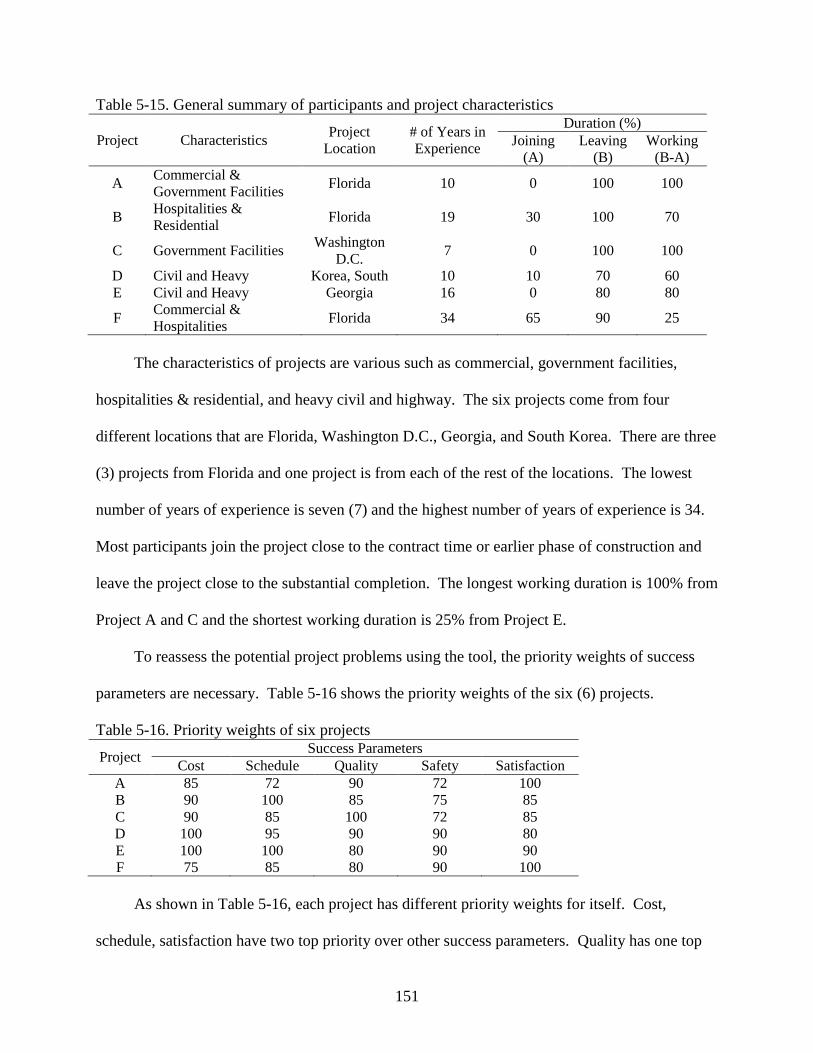
151
Table 5-15. General summary of participants and project characteristics
Project Characteristics Project
Location
# of Years in
Experience
Duration (%)
Joining
(A)
Leaving
(B)
Working
(B-A)
A Commercial &
Government Facilities Florida 10 0 100 100
B Hospitalities &
Residential Florida 19 30 100 70
C Government Facilities Washington
D.C. 7 0 100 100
D Civil and Heavy Korea, South 10 10 70 60
E Civil and Heavy Georgia 16 0 80 80
F Commercial &
Hospitalities Florida 34 65 90 25
The characteristics of projects are various such as commercial, government facilities,
hospitalities & residential, and heavy civil and highway. The six projects come from four
different locations that are Florida, Washington D.C., Georgia, and South Korea. There are three
(3) projects from Florida and one project is from each of the rest of the locations. The lowest
number of years of experience is seven (7) and the highest number of years of experience is 34.
Most participants join the project close to the contract time or earlier phase of construction and
leave the project close to the substantial completion. The longest working duration is 100% from
Project A and C and the shortest working duration is 25% from Project E.
To reassess the potential project problems using the tool, the priority weights of success
parameters are necessary. Table 5-16 shows the priority weights of the six (6) projects.
Table 5-16. Priority weights of six projects
Project Success Parameters
Cost Schedule Quality Safety Satisfaction
A 85 72 90 72 100
B 90 100 85 75 85
C 90 85 100 72 85
D 100 95 90 90 80
E 100 100 80 90 90
F 75 85 80 90 100
As shown in Table 5-16, each project has different priority weights for itself. Cost,
schedule, satisfaction have two top priority over other success parameters. Quality has one top
152
priority over other parameters. Safety has no top priority over other parameters and most of
them are marked as the lowest priority. Table 5-16 shows that each project has its own priorities
for project success. It supports that there should be more research on the multi-project success
parameters. Due to the variety of priority weights for success parameters and the number of
success parameters involved for a project, the current norm for the project control concept may
not be as accurate as it used to be. The current norm is as usual concerned about cost and
schedule. But now there are more parameters other than just cost and schedule to be considered
in classifying a project as successful in the construction industry.
The severity of the project problems of the six projects is shown in Table 5-17. The final
critical ranking in the project review process or the time a participant leaves a project and the
critical ranking computing from the application are shown in Table 5-17 as well. The highest
severity is 100 for Project E and F. The problem groups are CO and PC for Project E and CA for
Project F. The lowest severity is zero (0) for SP in Project A. The „Review‟ column shows the
critical ranking marked by the participant and the „Tool‟ column is the computed critical ranking
using the tool based on the survey input. The „Difference‟ column shows the difference in
ranking.
The easiest way to validate the tool is to compare the actual critical ranking assigned by a
participant to the critical ranking resulting from the tool based upon the survey input. If the tool
output is close to the actual output, then it will be a good validation of tool. If the output of tool
were perfectly the same as the actual ranking, then the values in „Difference‟ column of Table 5-
17 will be zero (0). Even though the output from the tool is not exactly the same as the actual
ranking, the output of the tool will be still validated if the values in the „Difference‟ column in
Table 5-17 are smaller. For example, a ranking from the tool is eighth and an actual ranking
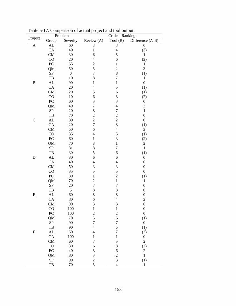
153
Table 5-17. Comparison of actual project and tool output
Project Problem Critical Ranking
Group Severity Review (A) Tool (B) Difference (A-B)
A AL 60 3 3 0
CA 40 1 4 (3)
CM 30 6 5 1
CO 20 4 6 (2)
PC 65 2 1 1
QM 50 5 2 3
SP 0 7 8 (1)
TB 10 8 7 1
B AL 90 1 1 0
CA 20 4 5 (1)
CM 20 5 6 (1)
CO 10 6 8 (2)
PC 60 3 3 0
QM 40 7 4 3
SP 20 8 7 1
TB 70 2 2 0
C AL 80 2 2 0
CA 20 7 8 (1)
CM 50 6 4 2
CO 35 4 5 (1)
PC 60 1 3 (2)
QM 70 3 1 2
SP 31 8 7 1
TB 30 5 6 (1)
D AL 30 6 6 0
CA 40 4 4 0
CM 50 3 3 0
CO 35 5 5 0
PC 80 1 2 (1)
QM 70 2 1 1
SP 20 7 7 0
TB 5 8 8 0
E AL 60 8 8 0
CA 80 6 4 2
CM 90 3 3 0
CO 100 1 1 0
PC 100 2 2 0
QM 70 5 6 (1)
SP 90 7 7 0
TB 90 4 5 (1)
F AL 50 4 7 (3)
CA 100 1 1 0
CM 60 7 5 2
CO 30 6 8 (2)
PC 40 8 6 2
QM 80 3 2 1
SP 90 2 3 (1)
TB 70 5 4 1
154
is first for a problem group. The ranking difference will be seven. This is the maximum ranking
difference between actual and tool output. In this case, the tool output may not be validated
because the gap between actual and tool output is much different. But if the ranking difference
between actual review and tool output is small enough such as one (1) or two (2), then the output
of tool is still considered to being close enough to the actual ranking. The values in the
„Difference‟ column in Table 5-17 have the minimum of zero (0) and the maximum of three (3)
in absolute value form. Only four problem groups have a three (3) difference out of 48 problem
groups could be found and the rest of values in differences fall in the zero (0), one (1), or two
(2) groups. The output of the tool predicts very close the actual ones.
In addition to the ranking difference between tool output and actual output for the
validation of the tool, another way to validate the tool is to use a regression model. The
evaluation of a regression model is to use the R2 value (variability). The higher the R
2 value, the
better the validation is for the model. A regression model for this case falls into the expectation
or forecasting model. If all the values of actual critical ranking in Table 5-17 are on the y-axis
and the values of tool critical rankings in Table 5-17 are on the x-axis, then a regression model
with R2 can be drawn as shown in Figure 5-7. The R
2 value of this regression model is 0.6747
(67.47%). It is not a high R2 value but it is still serves validating the tool. The equation of this
regression model is shown in Equation 5-1:
y = 0.8214x + 0.8036 (Equation 5-1)
where, y=actual critical ranking; x= tool critical ranking.
Even though there is a small difference in critical ranking as shown in Table 5-17, the R2 value
does not seem high. This is because the four (4) combination pairs of ranking have a difference
of three (3), CA and QM in Project A, QM in Project B, and AL in Project F in Table 5-17.
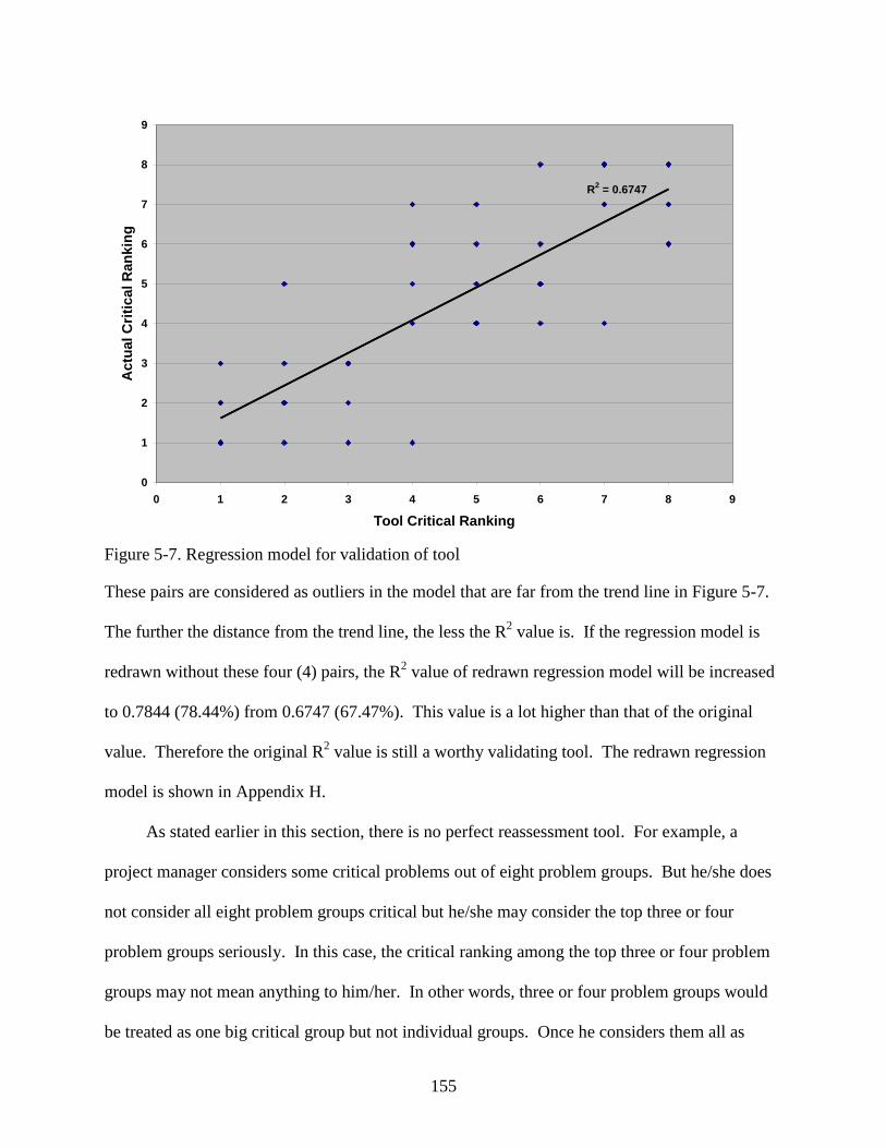
155
R2 = 0.6747
0
1
2
3
4
5
6
7
8
9
0 1 2 3 4 5 6 7 8 9
Tool Critical Ranking
Actu
al
Cri
tic
al
Ran
kin
g
Figure 5-7. Regression model for validation of tool
These pairs are considered as outliers in the model that are far from the trend line in Figure 5-7.
The further the distance from the trend line, the less the R2 value is. If the regression model is
redrawn without these four (4) pairs, the R2 value of redrawn regression model will be increased
to 0.7844 (78.44%) from 0.6747 (67.47%). This value is a lot higher than that of the original
value. Therefore the original R2 value is still a worthy validating tool. The redrawn regression
model is shown in Appendix H.
As stated earlier in this section, there is no perfect reassessment tool. For example, a
project manager considers some critical problems out of eight problem groups. But he/she does
not consider all eight problem groups critical but he/she may consider the top three or four
problem groups seriously. In this case, the critical ranking among the top three or four problem
groups may not mean anything to him/her. In other words, three or four problem groups would
be treated as one big critical group but not individual groups. Once he considers them all as

156
critical. From this perspective, the output of this tool is able to provide an overview of the
critical problem groups based on the situations. Although, based on six case studies, this tool is
not perfectly the same as the actual ranking, it still will be able to provide the potential
assessment of project problems with a priority weight of success parameters.
157
CHAPTER 6
CONCLUSIONS AND RECOMMENDATIONS
Conclusions
Our society is getting more demanding in every aspect of our lives as technology has
developed and our way of life has improved. It is hard for sellers or service providers to satisfy
customers due to the high expectation from customers on the service. From this perspective, the
construction industry has been changing rapidly as well. The customers (owners) have more
demands on their service (construction) and the service providers (general contractors) try to
keep the customers satisfied to have them come again for another service (repeat customers).
The demands on service in construction come from two perspectives in terms of time. One is for
the construction phase and something tangible and objective and the other is after the
construction and something intangible and subjective. Within the five project success
parameters, the first one is related to cost, schedule, and safety, while the second one is related to
quality and satisfaction. Traditionally, cost and schedule are two favorite success parameters
used for construction projects in order to classify them as a successful project. As discussed
based on Table 5-16 most projects require more than cost and schedule to be successful with
different priority weights. The priority weights depend heavily upon owners‟ requests and the
characteristics of projects. It depicts a project manager‟s concern for all possible success
parameters to meet the owner‟s demands and at the same time minimize the potential for current
problems, in order to deliver a successful project. How well project problems are managed is the
key to satisfying the customers. To do so, it is necessary to research the relationship between
project success parameters and project problems and to integrate them as one project control and
management perspective.
158
Many articles have been written about project management and controls and most of them
are focused on cost and schedule as keys to success. These two parameters are clearly an
objective measurement to judge the success of a project. This could be why many studies on
cost and schedule have been conducted. On the other hand, there are not so many studies
available on other parameters for project success. Besides cost and schedule, safety, quality, and
satisfaction could be used, but they are subjective and they can be difficult to measure. Even
though these parameters would be subjective and hard to measure, the request to satisfy these
parameters in addition to cost and schedule are rising in the construction industry as shown in the
data gathered in Table 5-16. In this study, the relationship between project success parameters
and project problems are mainly discussed using various methods such as canonical correlations
and factor analysis. During this process, project problems respond to each project success
parameter differently. Their responses are not constant for the five project success parameters.
Once the relationship between a project success parameter and project problems are defined
using confirmatory factor analysis (CFA), this study performs the integration of five project
success parameters as one project success parameter depending on their priority weights. To
accomplish this, the SMARTS (Edwards and Barron 1994) technique is applied. During this
integration of the five project success parameters with their priority weights, all the relationships
between a project success parameter and project problems are integrated as well. Based on the
priority weights of the project success parameters, the potential critical problem groups can be
identified. Lastly, the degree of problem severity is applied to the previous stage to reassess the
critical project problem groups at the early phase of construction or earlier than that. Using this
process, the project manager could identify the critical problem groups using the priority weights
of the success parameters and the degree of problem severity the project faces.
159
The final output of this research is a simple measurement tool called Potential Problem
Identification Tool. This tool is a decision-making aid for project managers at the early phase of
a project. The tool gives you a degree of overview for being critical of project problems based
on priority weights of success parameters and the degree of project problem severity. It will be
helpful to projects managers in managing project problems when there are limited resources
available to manage them. As mentioned in the validation process, this is a good guideline for a
decision-making tool but not an absolute way for the selection of critical problem groups.
Combining personal experience and this tool would result in the best selection of critical
problems for a project.
Recommendations for Future Research
This research mainly concerns the relationships between project problems and project
success parameters and its application. This study is not the first study of multi-project success
parameters, but one of a few studies done so far. All the processes addressed in this study will
be helpful for further studies on multi-project success parameters. There are five project success
parameters discussed in this study and there could be more than five and possibly other kinds of
parameters available.
Regarding project problem groups, this research focuses on the project problem group
level but it may be necessary to study these relationships at the project problem level as well.
Even though the project group level provides the overview of relationship between problem
groups and success parameters, with respect to the applications of the results, there would be
more potential ways at the project problem level, compared to the project group level. It will
give more opportunities to study the relationship between project success parameters and
problems in depth and provides more versatility in its application. If both project problem group
level and project problem level are available, then the project problem group level would be
160
useful for the early phase of project to set up the overall direction of project. On the other hand,
the project problem level would be useful for the project control during the whole period of
project execution.
The main concept of the identification tool is to decide the weight of the priority of success
parameters and to identify the degree of severity. Even though it is designed to assist a project
manager in the decision-making process for the selection of critical problem groups under the
given circumstances, the weights for success parameters and the degree of severity may not be
the same among all project participants in the same project if all participants are asked to decide
the weights of success parameters and the degree of severity because everybody has their own
perspective of a project and interprets it in their ways. In this case, the output of a tool can be
different for different participants. To minimize this discrepancy on perceptions for the usage of
tool among project participants, even it is recommended that fuzzy weighting (Seo et al. 2004)
investigated for ranking the priority of weights and the severity of problems. This could possibly
result in less biased output to choose from for the project manager.
One of the objectives of this research is to define the relationship between project problems
and project success parameters. Through this relationship, this research provides the guideline in
identifying the potential project problems using the priorities of success weights and the degree
of problem severities. The identification of potential problem groups for the project is a part of
the project risk mitigation plans. The project risk is different for different project contracting
strategies and project delivery methods. It means a problem does not have the same degree of
negative impact for every contracting strategy and project delivery method all the time. A
negative impact of a problem on a project in a lump sum contract may not be the same as the one
in a cost plus contract. In addition to contracting strategy and project delivery, the project types

161
will be considered as well. A different type of project such as commercial, residential, industry,
and heavy civil has its own characteristics to be concerned for a project success. If every type of
project has a problem, then the negative impact of that problem cannot be the same to all
different types of project because its impact on project could be different from the type of
projects. The final output and application of the output for this research would be a boilerplate,
but not a tailor-made for a specific type of contracting strategy, project delivery method, or
project type. These issues should be explored in future studies, This research mainly focuses on
the projects and practices in the United Sates. Every country has different culture and practices.
It means that the output of current tool for a foreign country may not be as useful as here. With
respect to the globalization, the research on overseas projects would provide deep insight into
international project management.
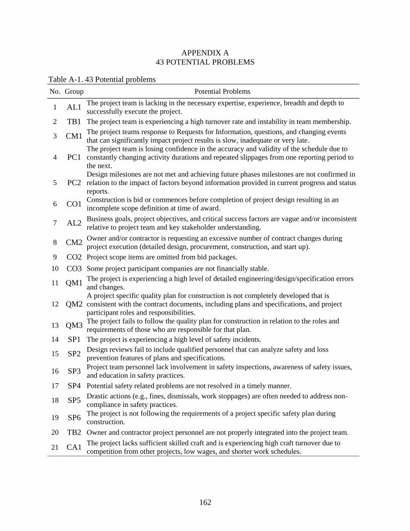
162
APPENDIX A
43 POTENTIAL PROBLEMS
Table A-1. 43 Potential problems
No. Group Potential Problems
1 AL1 The project team is lacking in the necessary expertise, experience, breadth and depth to
successfully execute the project.
2 TB1 The project team is experiencing a high turnover rate and instability in team membership.
3 CM1 The project teams response to Requests for Information, questions, and changing events
that can significantly impact project results is slow, inadequate or very late.
4 PC1 The project team is losing confidence in the accuracy and validity of the schedule due to
constantly changing activity durations and repeated slippages from one reporting period to
the next.
5 PC2 Design milestones are not met and achieving future phases milestones are not confirmed in
relation to the impact of factors beyond information provided in current progress and status
reports.
6 CO1 Construction is bid or commences before completion of project design resulting in an
incomplete scope definition at time of award.
7 AL2 Business goals, project objectives, and critical success factors are vague and/or inconsistent
relative to project team and key stakeholder understanding.
8 CM2 Owner and/or contractor is requesting an excessive number of contract changes during
project execution (detailed design, procurement, construction, and start up).
9 CO2 Project scope items are omitted from bid packages.
10 CO3 Some project participant companies are not financially stable.
11 QM1 The project is experiencing a high level of detailed engineering/design/specification errors
and changes.
12 QM2 A project specific quality plan for construction is not completely developed that is
consistent with the contract documents, including plans and specifications, and project
participant roles and responsibilities.
13 QM3 The project fails to follow the quality plan for construction in relation to the roles and
requirements of those who are responsible for that plan.
14 SP1 The project is experiencing a high level of safety incidents.
15 SP2 Design reviews fail to include qualified personnel that can analyze safety and loss
prevention features of plans and specifications.
16 SP3 Project team personnel lack involvement in safety inspections, awareness of safety issues,
and education in safety practices.
17 SP4 Potential safety related problems are not resolved in a timely manner.
18 SP5 Drastic actions (e.g., fines, dismissals, work stoppages) are often needed to address non-
compliance in safety practices.
19 SP6 The project is not following the requirements of a project specific safety plan during
construction.
20 TB2 Owner and contractor project personnel are not properly integrated into the project team.
21 CA1 The project lacks sufficient skilled craft and is experiencing high craft turnover due to
competition from other projects, low wages, and shorter work schedules.
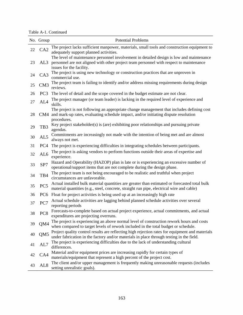
163
Table A-1. Continued
No. Group Potential Problems
22 CA2 The project lacks sufficient manpower, materials, small tools and construction equipment to
adequately support planned activities.
23 AL3 The level of maintenance personnel involvement in detailed design is low and maintenance
personnel are not aligned with other project team personnel with respect to maintenance
issues for the facility.
24 CA3 The project is using new technology or construction practices that are unproven in
commercial use.
25 CM3 The project team is failing to identify and/or address missing requirements during design
reviews.
26 PC3 The level of detail and the scope covered in the budget estimate are not clear.
27 AL4 The project manager (or team leader) is lacking in the required level of experience and
skills.
28 CM4 The project is not following an appropriate change management that includes defining cost
and mark-up rates, evaluating schedule impact, and/or initiating dispute resolution
procedures.
29 TB3 Key project stakeholder(s) is (are) exhibiting poor relationships and pursuing private
agendas.
30 AL5 Commitments are increasingly not made with the intention of being met and are almost
always not met.
31 PC4 The project is experiencing difficulties in integrating schedules between participants.
32 AL6 The project is asking vendors to perform functions outside their areas of expertise and
experience.
33 SP7 Hazard and Operability (HAZOP) plan is late or is experiencing an excessive number of
operational/support items that are not complete during the design phase.
34 TB4 The project team is not being encouraged to be realistic and truthful when project
circumstances are unfavorable.
35 PC5 Actual installed bulk material quantities are greater than estimated or forecasted total bulk
material quantities (e.g., steel, concrete, straight run pipe, electrical wire and cable)
36 PC6 Float for project activities is being used up at an increasingly high rate
37 PC7 Actual schedule activities are lagging behind planned schedule activities over several
reporting periods
38 PC8 Forecasts-to-complete based on actual project experience, actual commitments, and actual
expenditures are projecting overruns.
39 QM4 The project is experiencing an above normal level of construction rework hours and costs
when compared to target levels of rework included in the total budget or schedule.
40 QM5 Project quality control results are reflecting high rejection rates for equipment and materials
under fabrication in the factory and/or materials in place through testing in the field.
41 AL7 The project is experiencing difficulties due to the lack of understanding cultural
differences.
42 CA4 Material and/or equipment prices are increasing rapidly for certain types of
materials/equipment that represent a high percent of the project cost.
43 AL8 The client and/or upper management is frequently making unreasonable requests (includes
setting unrealistic goals).
164
APPENDIX B
DEFINITION OF EACH PROBLEM GROUP
Alignment (AL): These are practices associated with the overall alignment of the project team
with respect to project goals and objectives. The make-up of project teams can change
considerably from the Pre-Project Planning Phase to the Execution Phase. The owner project
team generally changes from business planning personnel to those responsible for
implementation. New contractors and suppliers are also usually added at this time. Both
owner and contractor teams are generally expanded to address the increasing volume of work.
How these new team members and contractors understand and are aligned to common goals
plays key role to project success.
Constructability (CA): Constructability generally involves construction related methodology
and planning. The ability to efficiently plan and execute the construction of a facility is a
major driver behind project success.
Change Management (CM): CII and others have accumulated large amounts of research
regarding the effects of late project scope changes and high volumes of rework to poor project
outcomes. How the project team makes decisions on, controls, tracks, and implements change
on a project can have a significant effect on project outcomes.
Contracting (CO): Contracting in terms of a practice is based on the matching of contract types
to project risks. It is not an endorsement of any one particular contract type. There is no
weighting of the tool that values Turnkey versus Lump Sum versus Design-Build versus Cost
Reimbursable. It is purely a measure of whether the project team is seeing potential issues
between the contracts in place and the scope that needs to be executed.
Project Control (PC): Project control involves the tools and techniques used to track, evaluate
and improve schedule and cost performance. In terms of this tool, it is not simply the use of a
project schedule and cost reporting. It is a measure of how accurate the schedule is; how
effective the schedule is in tracking work and identifying gaps; whether the cost reporting is
utilized in future decision making; and whether or not the team is effectively using the
information as a planning tool. Too often, schedule and cost reports become deliverables
themselves instead of tools to be used in planning the work.
Quality Management (QM): Quality Management includes items such as quality of engineering,
construction quality and rework, equipment inspections and testing and facility start-up.
Safety Practices (SP): This is a measure of whether or not the project team is fully engaged in
the practices that drive project safety (see CII Target Zero practices).
Team Building (TB): People implement projects. The core competencies of the people that
constitute the project team and how the people that make-up the project team play a very key
role in the success of any project. Good project teams overcome gaps in scope, risk events,
design issues, project changes etc., in a proactive way to minimize the negative effects on
project outcomes. Poor teams do not.
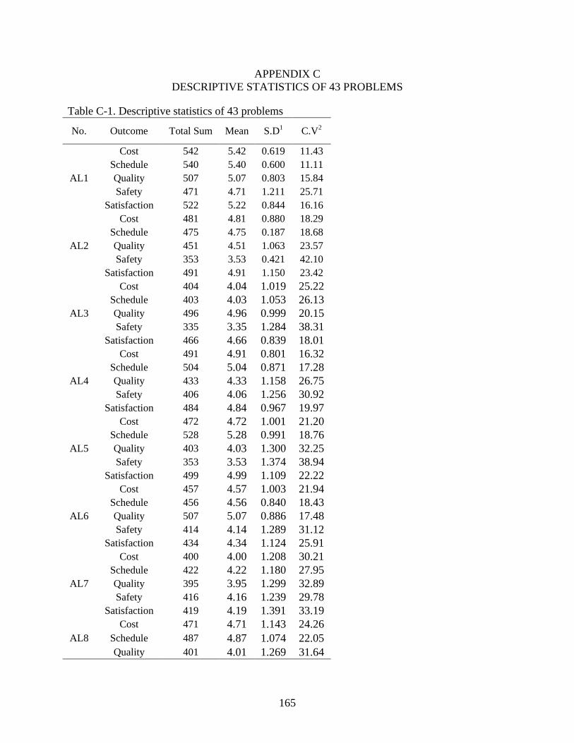
165
APPENDIX C
DESCRIPTIVE STATISTICS OF 43 PROBLEMS
Table C-1. Descriptive statistics of 43 problems
No. Outcome Total Sum Mean S.D1 C.V
2
AL1
Cost 542 5.42 0.619 11.43
Schedule 540 5.40 0.600 11.11
Quality 507 5.07 0.803 15.84
Safety 471 4.71 1.211 25.71
Satisfaction 522 5.22 0.844 16.16
AL2
Cost 481 4.81 0.880 18.29
Schedule 475 4.75 0.187 18.68
Quality 451 4.51 1.063 23.57
Safety 353 3.53 0.421 42.10
Satisfaction 491 4.91 1.150 23.42
AL3
Cost 404 4.04 1.019 25.22
Schedule 403 4.03 1.053 26.13
Quality 496 4.96 0.999 20.15
Safety 335 3.35 1.284 38.31
Satisfaction 466 4.66 0.839 18.01
AL4
Cost 491 4.91 0.801 16.32
Schedule 504 5.04 0.871 17.28
Quality 433 4.33 1.158 26.75
Safety 406 4.06 1.256 30.92
Satisfaction 484 4.84 0.967 19.97
AL5
Cost 472 4.72 1.001 21.20
Schedule 528 5.28 0.991 18.76
Quality 403 4.03 1.300 32.25
Safety 353 3.53 1.374 38.94
Satisfaction 499 4.99 1.109 22.22
AL6
Cost 457 4.57 1.003 21.94
Schedule 456 4.56 0.840 18.43
Quality 507 5.07 0.886 17.48
Safety 414 4.14 1.289 31.12
Satisfaction 434 4.34 1.124 25.91
AL7
Cost 400 4.00 1.208 30.21
Schedule 422 4.22 1.180 27.95
Quality 395 3.95 1.299 32.89
Safety 416 4.16 1.239 29.78
Satisfaction 419 4.19 1.391 33.19
AL8
Cost 471 4.71 1.143 24.26
Schedule 487 4.87 1.074 22.05
Quality 401 4.01 1.269 31.64
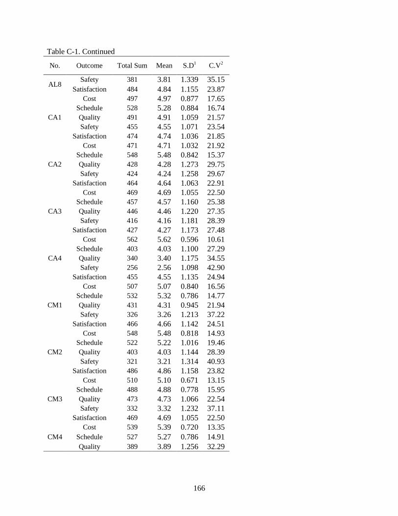
166
Table C-1. Continued
No. Outcome Total Sum Mean S.D1 C.V
2
AL8 Safety 381 3.81 1.339 35.15
Satisfaction 484 4.84 1.155 23.87
CA1
Cost 497 4.97 0.877 17.65
Schedule 528 5.28 0.884 16.74
Quality 491 4.91 1.059 21.57
Safety 455 4.55 1.071 23.54
Satisfaction 474 4.74 1.036 21.85
CA2
Cost 471 4.71 1.032 21.92
Schedule 548 5.48 0.842 15.37
Quality 428 4.28 1.273 29.75
Safety 424 4.24 1.258 29.67
Satisfaction 464 4.64 1.063 22.91
CA3
Cost 469 4.69 1.055 22.50
Schedule 457 4.57 1.160 25.38
Quality 446 4.46 1.220 27.35
Safety 416 4.16 1.181 28.39
Satisfaction 427 4.27 1.173 27.48
CA4
Cost 562 5.62 0.596 10.61
Schedule 403 4.03 1.100 27.29
Quality 340 3.40 1.175 34.55
Safety 256 2.56 1.098 42.90
Satisfaction 455 4.55 1.135 24.94
CM1
Cost 507 5.07 0.840 16.56
Schedule 532 5.32 0.786 14.77
Quality 431 4.31 0.945 21.94
Safety 326 3.26 1.213 37.22
Satisfaction 466 4.66 1.142 24.51
CM2
Cost 548 5.48 0.818 14.93
Schedule 522 5.22 1.016 19.46
Quality 403 4.03 1.144 28.39
Safety 321 3.21 1.314 40.93
Satisfaction 486 4.86 1.158 23.82
CM3
Cost 510 5.10 0.671 13.15
Schedule 488 4.88 0.778 15.95
Quality 473 4.73 1.066 22.54
Safety 332 3.32 1.232 37.11
Satisfaction 469 4.69 1.055 22.50
CM4
Cost 539 5.39 0.720 13.35
Schedule 527 5.27 0.786 14.91
Quality 389 3.89 1.256 32.29
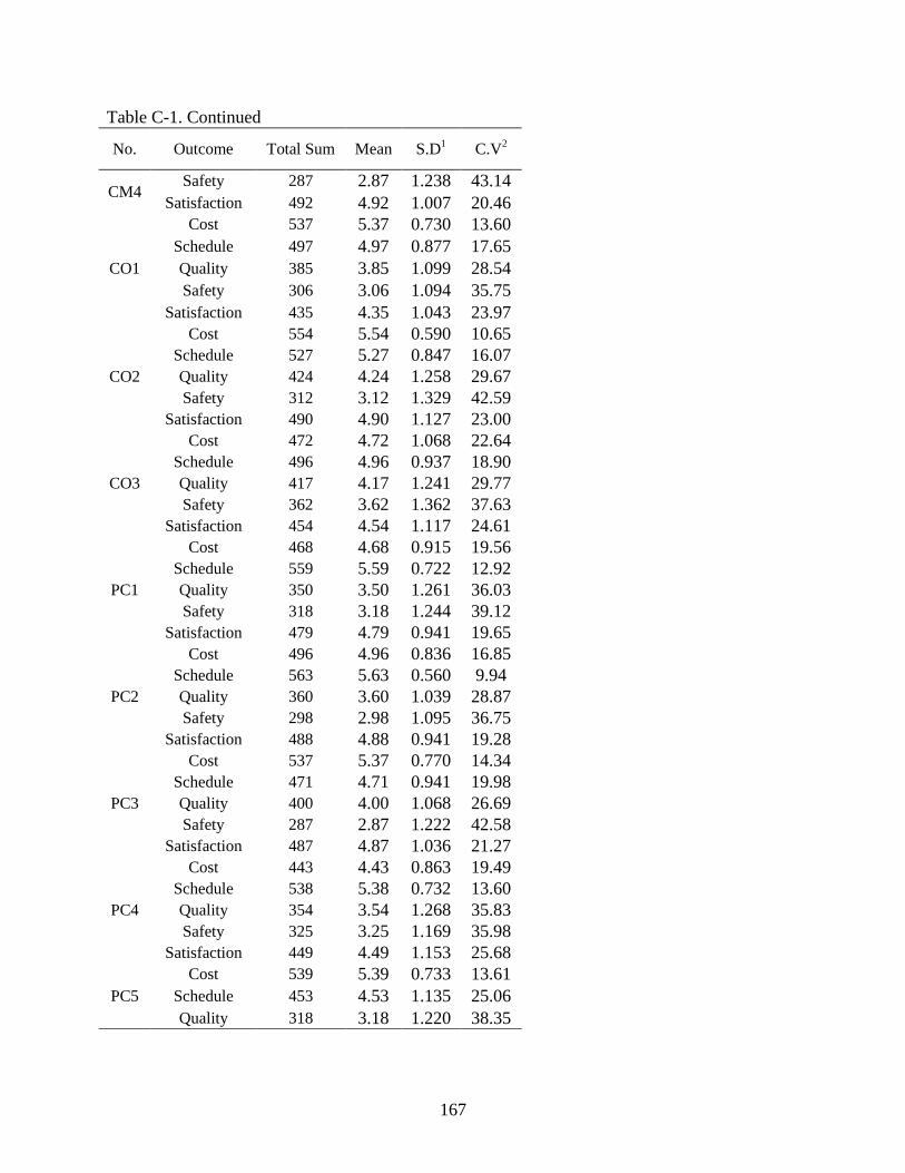
167
Table C-1. Continued
No. Outcome Total Sum Mean S.D1 C.V
2
CM4 Safety 287 2.87 1.238 43.14
Satisfaction 492 4.92 1.007 20.46
CO1
Cost 537 5.37 0.730 13.60
Schedule 497 4.97 0.877 17.65
Quality 385 3.85 1.099 28.54
Safety 306 3.06 1.094 35.75
Satisfaction 435 4.35 1.043 23.97
CO2
Cost 554 5.54 0.590 10.65
Schedule 527 5.27 0.847 16.07
Quality 424 4.24 1.258 29.67
Safety 312 3.12 1.329 42.59
Satisfaction 490 4.90 1.127 23.00
CO3
Cost 472 4.72 1.068 22.64
Schedule 496 4.96 0.937 18.90
Quality 417 4.17 1.241 29.77
Safety 362 3.62 1.362 37.63
Satisfaction 454 4.54 1.117 24.61
PC1
Cost 468 4.68 0.915 19.56
Schedule 559 5.59 0.722 12.92
Quality 350 3.50 1.261 36.03
Safety 318 3.18 1.244 39.12
Satisfaction 479 4.79 0.941 19.65
PC2
Cost 496 4.96 0.836 16.85
Schedule 563 5.63 0.560 9.94
Quality 360 3.60 1.039 28.87
Safety 298 2.98 1.095 36.75
Satisfaction 488 4.88 0.941 19.28
PC3
Cost 537 5.37 0.770 14.34
Schedule 471 4.71 0.941 19.98
Quality 400 4.00 1.068 26.69
Safety 287 2.87 1.222 42.58
Satisfaction 487 4.87 1.036 21.27
PC4
Cost 443 4.43 0.863 19.49
Schedule 538 5.38 0.732 13.60
Quality 354 3.54 1.268 35.83
Safety 325 3.25 1.169 35.98
Satisfaction 449 4.49 1.153 25.68
PC5
Cost 539 5.39 0.733 13.61
Schedule 453 4.53 1.135 25.06
Quality 318 3.18 1.220 38.35
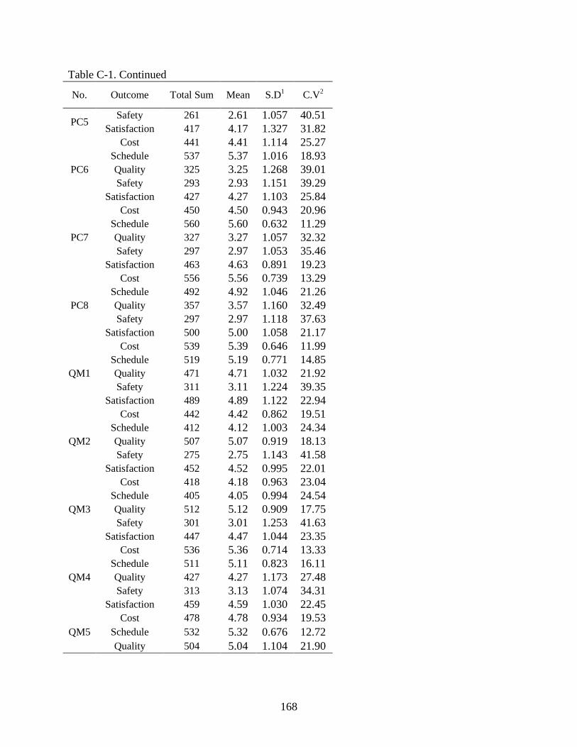
168
Table C-1. Continued
No. Outcome Total Sum Mean S.D1 C.V
2
PC5 Safety 261 2.61 1.057 40.51
Satisfaction 417 4.17 1.327 31.82
PC6
Cost 441 4.41 1.114 25.27
Schedule 537 5.37 1.016 18.93
Quality 325 3.25 1.268 39.01
Safety 293 2.93 1.151 39.29
Satisfaction 427 4.27 1.103 25.84
PC7
Cost 450 4.50 0.943 20.96
Schedule 560 5.60 0.632 11.29
Quality 327 3.27 1.057 32.32
Safety 297 2.97 1.053 35.46
Satisfaction 463 4.63 0.891 19.23
PC8
Cost 556 5.56 0.739 13.29
Schedule 492 4.92 1.046 21.26
Quality 357 3.57 1.160 32.49
Safety 297 2.97 1.118 37.63
Satisfaction 500 5.00 1.058 21.17
QM1
Cost 539 5.39 0.646 11.99
Schedule 519 5.19 0.771 14.85
Quality 471 4.71 1.032 21.92
Safety 311 3.11 1.224 39.35
Satisfaction 489 4.89 1.122 22.94
QM2
Cost 442 4.42 0.862 19.51
Schedule 412 4.12 1.003 24.34
Quality 507 5.07 0.919 18.13
Safety 275 2.75 1.143 41.58
Satisfaction 452 4.52 0.995 22.01
QM3
Cost 418 4.18 0.963 23.04
Schedule 405 4.05 0.994 24.54
Quality 512 5.12 0.909 17.75
Safety 301 3.01 1.253 41.63
Satisfaction 447 4.47 1.044 23.35
QM4
Cost 536 5.36 0.714 13.33
Schedule 511 5.11 0.823 16.11
Quality 427 4.27 1.173 27.48
Safety 313 3.13 1.074 34.31
Satisfaction 459 4.59 1.030 22.45
QM5
Cost 478 4.78 0.934 19.53
Schedule 532 5.32 0.676 12.72
Quality 504 5.04 1.104 21.90
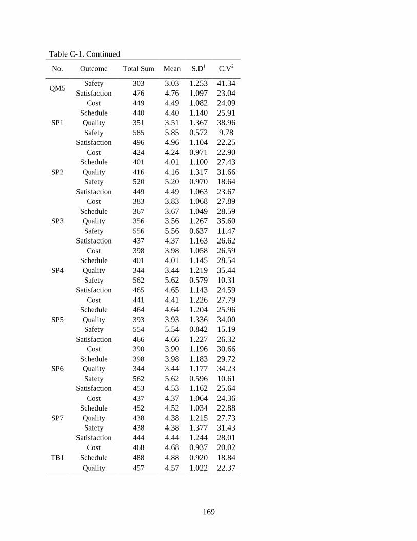
169
Table C-1. Continued
No. Outcome Total Sum Mean S.D1 C.V
2
QM5 Safety 303 3.03 1.253 41.34
Satisfaction 476 4.76 1.097 23.04
SP1
Cost 449 4.49 1.082 24.09
Schedule 440 4.40 1.140 25.91
Quality 351 3.51 1.367 38.96
Safety 585 5.85 0.572 9.78
Satisfaction 496 4.96 1.104 22.25
SP2
Cost 424 4.24 0.971 22.90
Schedule 401 4.01 1.100 27.43
Quality 416 4.16 1.317 31.66
Safety 520 5.20 0.970 18.64
Satisfaction 449 4.49 1.063 23.67
SP3
Cost 383 3.83 1.068 27.89
Schedule 367 3.67 1.049 28.59
Quality 356 3.56 1.267 35.60
Safety 556 5.56 0.637 11.47
Satisfaction 437 4.37 1.163 26.62
SP4
Cost 398 3.98 1.058 26.59
Schedule 401 4.01 1.145 28.54
Quality 344 3.44 1.219 35.44
Safety 562 5.62 0.579 10.31
Satisfaction 465 4.65 1.143 24.59
SP5
Cost 441 4.41 1.226 27.79
Schedule 464 4.64 1.204 25.96
Quality 393 3.93 1.336 34.00
Safety 554 5.54 0.842 15.19
Satisfaction 466 4.66 1.227 26.32
SP6
Cost 390 3.90 1.196 30.66
Schedule 398 3.98 1.183 29.72
Quality 344 3.44 1.177 34.23
Safety 562 5.62 0.596 10.61
Satisfaction 453 4.53 1.162 25.64
SP7
Cost 437 4.37 1.064 24.36
Schedule 452 4.52 1.034 22.88
Quality 438 4.38 1.215 27.73
Safety 438 4.38 1.377 31.43
Satisfaction 444 4.44 1.244 28.01
TB1
Cost 468 4.68 0.937 20.02
Schedule 488 4.88 0.920 18.84
Quality 457 4.57 1.022 22.37
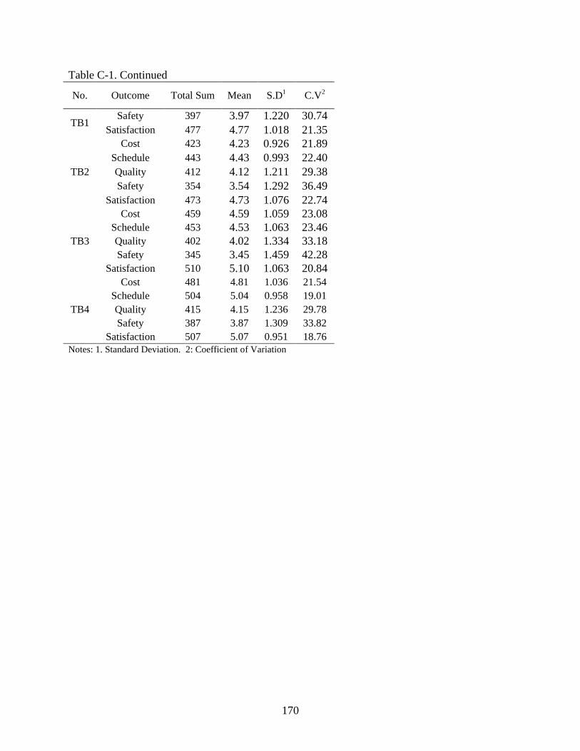
170
Table C-1. Continued
No. Outcome Total Sum Mean S.D1 C.V
2
TB1 Safety 397 3.97 1.220 30.74
Satisfaction 477 4.77 1.018 21.35
TB2
Cost 423 4.23 0.926 21.89
Schedule 443 4.43 0.993 22.40
Quality 412 4.12 1.211 29.38
Safety 354 3.54 1.292 36.49
Satisfaction 473 4.73 1.076 22.74
TB3
Cost 459 4.59 1.059 23.08
Schedule 453 4.53 1.063 23.46
Quality 402 4.02 1.334 33.18
Safety 345 3.45 1.459 42.28
Satisfaction 510 5.10 1.063 20.84
TB4
Cost 481 4.81 1.036 21.54
Schedule 504 5.04 0.958 19.01
Quality 415 4.15 1.236 29.78
Safety 387 3.87 1.309 33.82
Satisfaction 507 5.07 0.951 18.76
Notes: 1. Standard Deviation. 2: Coefficient of Variation
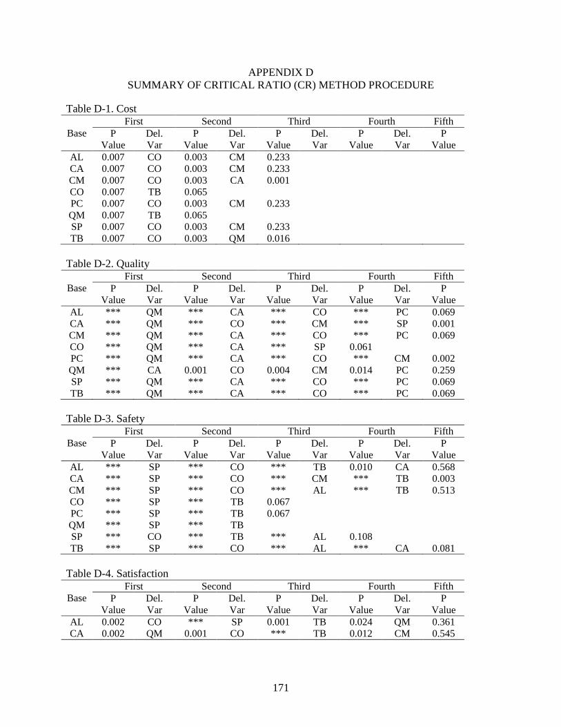
171
APPENDIX D
SUMMARY OF CRITICAL RATIO (CR) METHOD PROCEDURE
Table D-1. Cost
Base
First Second Third Fourth Fifth
P
Value
Del.
Var
P
Value
Del.
Var
P
Value
Del.
Var
P
Value
Del.
Var
P
Value
AL 0.007 CO 0.003 CM 0.233
CA 0.007 CO 0.003 CM 0.233
CM 0.007 CO 0.003 CA 0.001
CO 0.007 TB 0.065
PC 0.007 CO 0.003 CM 0.233
QM 0.007 TB 0.065
SP 0.007 CO 0.003 CM 0.233
TB 0.007 CO 0.003 QM 0.016
Table D-2. Quality
Base
First Second Third Fourth Fifth
P
Value
Del.
Var
P
Value
Del.
Var
P
Value
Del.
Var
P
Value
Del.
Var
P
Value
AL *** QM *** CA *** CO *** PC 0.069
CA *** QM *** CO *** CM *** SP 0.001
CM *** QM *** CA *** CO *** PC 0.069
CO *** QM *** CA *** SP 0.061
PC *** QM *** CA *** CO *** CM 0.002
QM *** CA 0.001 CO 0.004 CM 0.014 PC 0.259
SP *** QM *** CA *** CO *** PC 0.069
TB *** QM *** CA *** CO *** PC 0.069
Table D-3. Safety
Base
First Second Third Fourth Fifth
P
Value
Del.
Var
P
Value
Del.
Var
P
Value
Del.
Var
P
Value
Del.
Var
P
Value
AL *** SP *** CO *** TB 0.010 CA 0.568
CA *** SP *** CO *** CM *** TB 0.003
CM *** SP *** CO *** AL *** TB 0.513
CO *** SP *** TB 0.067
PC *** SP *** TB 0.067
QM *** SP *** TB
SP *** CO *** TB *** AL 0.108
TB *** SP *** CO *** AL *** CA 0.081
Table D-4. Satisfaction
Base
First Second Third Fourth Fifth
P
Value
Del.
Var
P
Value
Del.
Var
P
Value
Del.
Var
P
Value
Del.
Var
P
Value
AL 0.002 CO *** SP 0.001 TB 0.024 QM 0.361
CA 0.002 QM 0.001 CO *** TB 0.012 CM 0.545
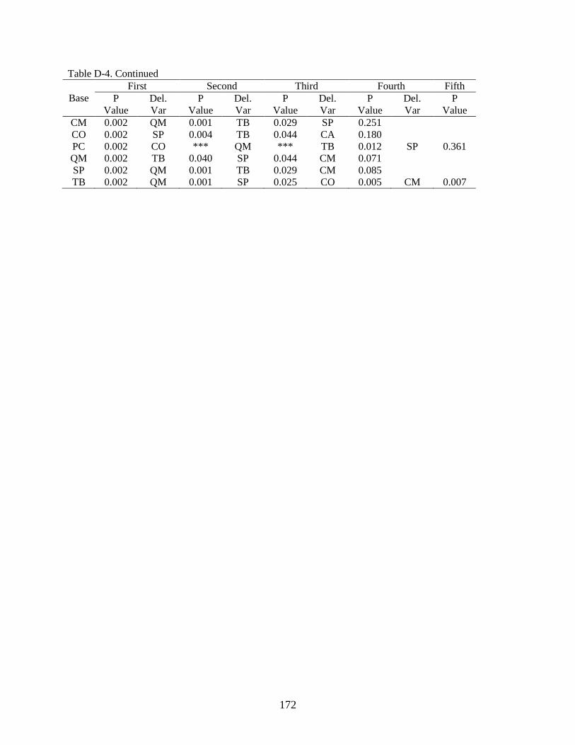
172
Table D-4. Continued
Base
First Second Third Fourth Fifth
P
Value
Del.
Var
P
Value
Del.
Var
P
Value
Del.
Var
P
Value
Del.
Var
P
Value
CM 0.002 QM 0.001 TB 0.029 SP 0.251
CO 0.002 SP 0.004 TB 0.044 CA 0.180
PC 0.002 CO *** QM *** TB 0.012 SP 0.361
QM 0.002 TB 0.040 SP 0.044 CM 0.071
SP 0.002 QM 0.001 TB 0.029 CM 0.085
TB 0.002 QM 0.001 SP 0.025 CO 0.005 CM 0.007
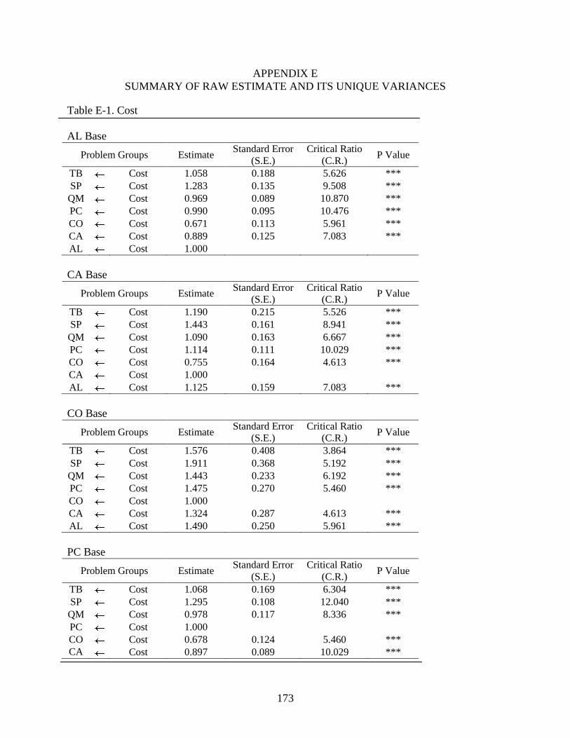
173
APPENDIX E
SUMMARY OF RAW ESTIMATE AND ITS UNIQUE VARIANCES
Table E-1. Cost
AL Base
Problem Groups Estimate Standard Error
(S.E.)
Critical Ratio
(C.R.) P Value
TB Cost 1.058 0.188 5.626 ***
SP Cost 1.283 0.135 9.508 ***
QM Cost 0.969 0.089 10.870 ***
PC Cost 0.990 0.095 10.476 ***
CO Cost 0.671 0.113 5.961 ***
CA Cost 0.889 0.125 7.083 ***
AL Cost 1.000
CA Base
Problem Groups Estimate Standard Error
(S.E.)
Critical Ratio
(C.R.) P Value
TB Cost 1.190 0.215 5.526 ***
SP Cost 1.443 0.161 8.941 ***
QM Cost 1.090 0.163 6.667 ***
PC Cost 1.114 0.111 10.029 ***
CO Cost 0.755 0.164 4.613 ***
CA Cost 1.000
AL Cost 1.125 0.159 7.083 ***
CO Base
Problem Groups Estimate Standard Error
(S.E.)
Critical Ratio
(C.R.) P Value
TB Cost 1.576 0.408 3.864 ***
SP Cost 1.911 0.368 5.192 ***
QM Cost 1.443 0.233 6.192 ***
PC Cost 1.475 0.270 5.460 ***
CO Cost 1.000
CA Cost 1.324 0.287 4.613 ***
AL Cost 1.490 0.250 5.961 ***
PC Base
Problem Groups Estimate Standard Error
(S.E.)
Critical Ratio
(C.R.) P Value
TB Cost 1.068 0.169 6.304 ***
SP Cost 1.295 0.108 12.040 ***
QM Cost 0.978 0.117 8.336 ***
PC Cost 1.000
CO Cost 0.678 0.124 5.460 ***
CA Cost 0.897 0.089 10.029 ***
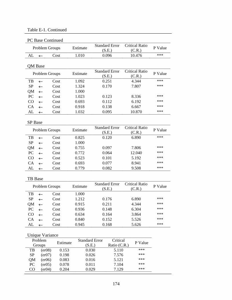
174
Table E-1. Continued
PC Base Continued
Problem Groups Estimate Standard Error
(S.E.)
Critical Ratio
(C.R.) P Value
AL Cost 1.010 0.096 10.476 ***
QM Base
Problem Groups Estimate Standard Error
(S.E.)
Critical Ratio
(C.R.) P Value
TB Cost 1.092 0.251 4.344 ***
SP Cost 1.324 0.170 7.807 ***
QM Cost 1.000
PC Cost 1.023 0.123 8.336 ***
CO Cost 0.693 0.112 6.192 ***
CA Cost 0.918 0.138 6.667 ***
AL Cost 1.032 0.095 10.870 ***
SP Base
Problem Groups Estimate Standard Error
(S.E.)
Critical Ratio
(C.R.) P Value
TB Cost 0.825 0.120 6.890 ***
SP Cost 1.000
QM Cost 0.755 0.097 7.806 ***
PC Cost 0.772 0.064 12.040 ***
CO Cost 0.523 0.101 5.192 ***
CA Cost 0.693 0.077 8.941 ***
AL Cost 0.779 0.082 9.508 ***
TB Base
Problem Groups Estimate Standard Error
(S.E.)
Critical Ratio
(C.R.) P Value
TB Cost 1.000
SP Cost 1.212 0.176 6.890 ***
QM Cost 0.915 0.211 4.344 ***
PC Cost 0.936 0.148 6.304 ***
CO Cost 0.634 0.164 3.864 ***
CA Cost 0.840 0.152 5.526 ***
AL Cost 0.945 0.168 5.626 ***
Unique Variance Problem
Groups Estimate
Standard Error
(S.E.)
Critical
Ratio (C.R.) P Value
TB (er08) 0.153 0.030 5.110 ***
SP (er07) 0.198 0.026 7.576 ***
QM (er06) 0.083 0.016 5.121 ***
PC (er05) 0.078 0.011 7.104 ***
CO (er04) 0.204 0.029 7.129 ***
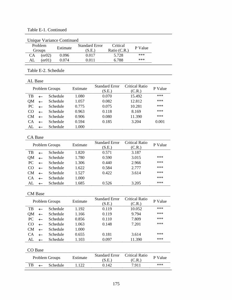
175
Table E-1. Continued
Unique Variance Continued Problem
Groups Estimate
Standard Error
(S.E.)
Critical
Ratio (C.R.) P Value
CA (er02) 0.096 0.017 5.728 ***
AL (er01) 0.074 0.011 6.788 ***
Table E-2. Schedule
AL Base
Problem Groups Estimate Standard Error
(S.E.)
Critical Ratio
(C.R.) P Value
TB Schedule 1.080 0.070 15.492 ***
QM Schedule 1.057 0.082 12.812 ***
PC Schedule 0.775 0.075 10.281 ***
CO Schedule 0.963 0.118 8.169 ***
CM Schedule 0.906 0.080 11.390 ***
CA Schedule 0.594 0.185 3.204 0.001
AL Schedule 1.000
CA Base
Problem Groups Estimate Standard Error
(S.E.)
Critical Ratio
(C.R.) P Value
TB Schedule 1.820 0.571 3.187
QM Schedule 1.780 0.590 3.015 ***
PC Schedule 1.306 0.440 2.966 ***
CO Schedule 1.622 0.584 2.777 ***
CM Schedule 1.527 0.422 3.614 ***
CA Schedule 1.000 ***
AL Schedule 1.685 0.526 3.205 ***
CM Base
Problem Groups Estimate Standard Error
(S.E.)
Critical Ratio
(C.R.) P Value
TB Schedule 1.192 0.119 10.052 ***
QM Schedule 1.166 0.119 9.794 ***
PC Schedule 0.856 0.110 7.809 ***
CO Schedule 1.063 0.148 7.201 ***
CM Schedule 1.000
CA Schedule 0.655 0.181 3.614 ***
AL Schedule 1.103 0.097 11.390 ***
CO Base
Problem Groups Estimate Standard Error
(S.E.)
Critical Ratio
(C.R.) P Value
TB Schedule 1.122 0.142 7.911 ***
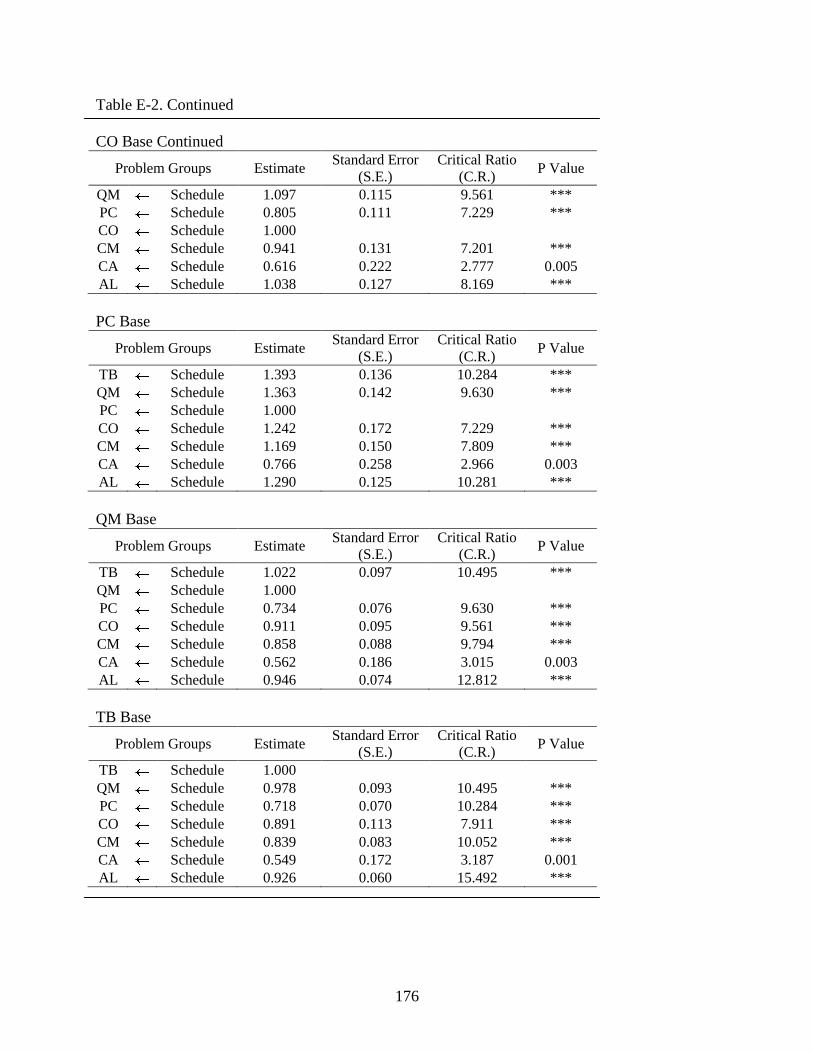
176
Table E-2. Continued
CO Base Continued
Problem Groups Estimate Standard Error
(S.E.)
Critical Ratio
(C.R.) P Value
QM Schedule 1.097 0.115 9.561 ***
PC Schedule 0.805 0.111 7.229 ***
CO Schedule 1.000
CM Schedule 0.941 0.131 7.201 ***
CA Schedule 0.616 0.222 2.777 0.005
AL Schedule 1.038 0.127 8.169 ***
PC Base
Problem Groups Estimate Standard Error
(S.E.)
Critical Ratio
(C.R.) P Value
TB Schedule 1.393 0.136 10.284 ***
QM Schedule 1.363 0.142 9.630 ***
PC Schedule 1.000
CO Schedule 1.242 0.172 7.229 ***
CM Schedule 1.169 0.150 7.809 ***
CA Schedule 0.766 0.258 2.966 0.003
AL Schedule 1.290 0.125 10.281 ***
QM Base
Problem Groups Estimate Standard Error
(S.E.)
Critical Ratio
(C.R.) P Value
TB Schedule 1.022 0.097 10.495 ***
QM Schedule 1.000
PC Schedule 0.734 0.076 9.630 ***
CO Schedule 0.911 0.095 9.561 ***
CM Schedule 0.858 0.088 9.794 ***
CA Schedule 0.562 0.186 3.015 0.003
AL Schedule 0.946 0.074 12.812 ***
TB Base
Problem Groups Estimate Standard Error
(S.E.)
Critical Ratio
(C.R.) P Value
TB Schedule 1.000
QM Schedule 0.978 0.093 10.495 ***
PC Schedule 0.718 0.070 10.284 ***
CO Schedule 0.891 0.113 7.911 ***
CM Schedule 0.839 0.083 10.052 ***
CA Schedule 0.549 0.172 3.187 0.001
AL Schedule 0.926 0.060 15.492 ***
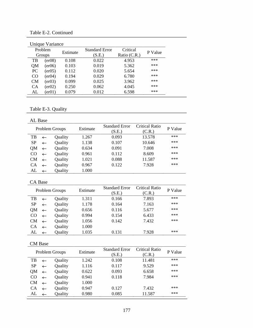
177
Table E-2. Continued
Unique Variance Problem
Groups Estimate
Standard Error
(S.E.)
Critical
Ratio (C.R.) P Value
TB (er08) 0.108 0.022 4.953 ***
QM (er06) 0.103 0.019 5.362 ***
PC (er05) 0.112 0.020 5.654 ***
CO (er04) 0.194 0.029 6.780 ***
CM (er03) 0.099 0.025 3.962 ***
CA (er02) 0.250 0.062 4.045 ***
AL (er01) 0.079 0.012 6.598 ***
Table E-3. Quality
AL Base
Problem Groups Estimate Standard Error
(S.E.)
Critical Ratio
(C.R.) P Value
TB Quality 1.267 0.093 13.578 ***
SP Quality 1.138 0.107 10.646 ***
QM Quality 0.634 0.091 7.008 ***
CO Quality 0.961 0.112 8.609 ***
CM Quality 1.021 0.088 11.587 ***
CA Quality 0.967 0.122 7.928 ***
AL Quality 1.000
CA Base
Problem Groups Estimate Standard Error
(S.E.)
Critical Ratio
(C.R.) P Value
TB Quality 1.311 0.166 7.893 ***
SP Quality 1.178 0.164 7.163 ***
QM Quality 0.656 0.116 5.677 ***
CO Quality 0.994 0.154 6.433 ***
CM Quality 1.056 0.142 7.432 ***
CA Quality 1.000
AL Quality 1.035 0.131 7.928 ***
CM Base
Problem Groups Estimate Standard Error
(S.E.)
Critical Ratio
(C.R.) P Value
TB Quality 1.242 0.108 11.481 ***
SP Quality 1.116 0.117 9.529 ***
QM Quality 0.622 0.093 6.658 ***
CO Quality 0.941 0.118 7.984 ***
CM Quality 1.000
CA Quality 0.947 0.127 7.432 ***
AL Quality 0.980 0.085 11.587 ***
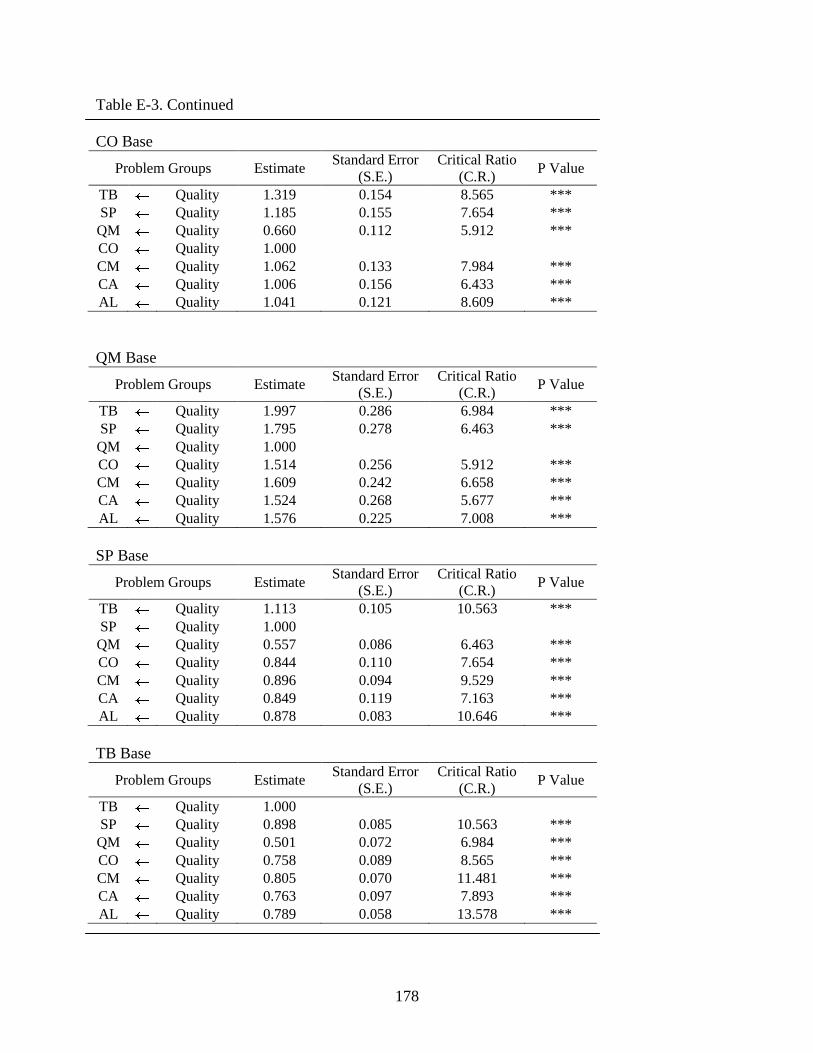
178
Table E-3. Continued
CO Base
Problem Groups Estimate Standard Error
(S.E.)
Critical Ratio
(C.R.) P Value
TB Quality 1.319 0.154 8.565 ***
SP Quality 1.185 0.155 7.654 ***
QM Quality 0.660 0.112 5.912 ***
CO Quality 1.000
CM Quality 1.062 0.133 7.984 ***
CA Quality 1.006 0.156 6.433 ***
AL Quality 1.041 0.121 8.609 ***
QM Base
Problem Groups Estimate Standard Error
(S.E.)
Critical Ratio
(C.R.) P Value
TB Quality 1.997 0.286 6.984 ***
SP Quality 1.795 0.278 6.463 ***
QM Quality 1.000
CO Quality 1.514 0.256 5.912 ***
CM Quality 1.609 0.242 6.658 ***
CA Quality 1.524 0.268 5.677 ***
AL Quality 1.576 0.225 7.008 ***
SP Base
Problem Groups Estimate Standard Error
(S.E.)
Critical Ratio
(C.R.) P Value
TB Quality 1.113 0.105 10.563 ***
SP Quality 1.000
QM Quality 0.557 0.086 6.463 ***
CO Quality 0.844 0.110 7.654 ***
CM Quality 0.896 0.094 9.529 ***
CA Quality 0.849 0.119 7.163 ***
AL Quality 0.878 0.083 10.646 ***
TB Base
Problem Groups Estimate Standard Error
(S.E.)
Critical Ratio
(C.R.) P Value
TB Quality 1.000
SP Quality 0.898 0.085 10.563 ***
QM Quality 0.501 0.072 6.984 ***
CO Quality 0.758 0.089 8.565 ***
CM Quality 0.805 0.070 11.481 ***
CA Quality 0.763 0.097 7.893 ***
AL Quality 0.789 0.058 13.578 ***
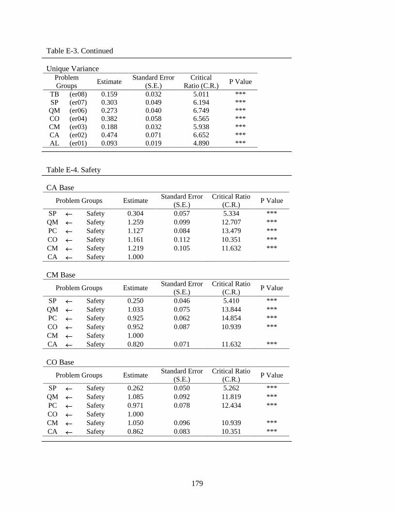
179
Table E-3. Continued
Unique Variance Problem
Groups Estimate
Standard Error
(S.E.)
Critical
Ratio (C.R.) P Value
TB (er08) 0.159 0.032 5.011 ***
SP (er07) 0.303 0.049 6.194 ***
QM (er06) 0.273 0.040 6.749 ***
CO (er04) 0.382 0.058 6.565 ***
CM (er03) 0.188 0.032 5.938 ***
CA (er02) 0.474 0.071 6.652 ***
AL (er01) 0.093 0.019 4.890 ***
Table E-4. Safety
CA Base
Problem Groups Estimate Standard Error
(S.E.)
Critical Ratio
(C.R.) P Value
SP Safety 0.304 0.057 5.334 ***
QM Safety 1.259 0.099 12.707 ***
PC Safety 1.127 0.084 13.479 ***
CO Safety 1.161 0.112 10.351 ***
CM Safety 1.219 0.105 11.632 ***
CA Safety 1.000
CM Base
Problem Groups Estimate Standard Error
(S.E.)
Critical Ratio
(C.R.) P Value
SP Safety 0.250 0.046 5.410 ***
QM Safety 1.033 0.075 13.844 ***
PC Safety 0.925 0.062 14.854 ***
CO Safety 0.952 0.087 10.939 ***
CM Safety 1.000
CA Safety 0.820 0.071 11.632 ***
CO Base
Problem Groups Estimate Standard Error
(S.E.)
Critical Ratio
(C.R.) P Value
SP Safety 0.262 0.050 5.262 ***
QM Safety 1.085 0.092 11.819 ***
PC Safety 0.971 0.078 12.434 ***
CO Safety 1.000
CM Safety 1.050 0.096 10.939 ***
CA Safety 0.862 0.083 10.351 ***
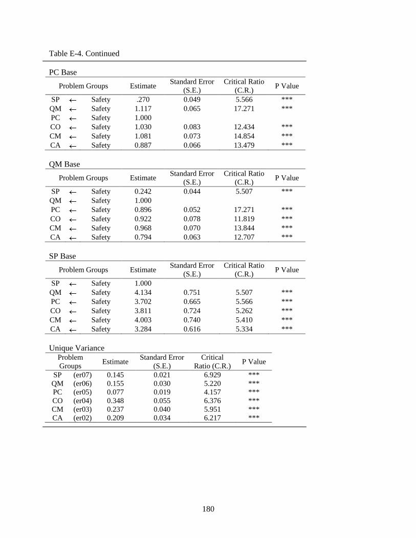
180
Table E-4. Continued
PC Base
Problem Groups Estimate Standard Error
(S.E.)
Critical Ratio
(C.R.) P Value
SP Safety .270 0.049 5.566 ***
QM Safety 1.117 0.065 17.271 ***
PC Safety 1.000
CO Safety 1.030 0.083 12.434 ***
CM Safety 1.081 0.073 14.854 ***
CA Safety 0.887 0.066 13.479 ***
QM Base
Problem Groups Estimate Standard Error
(S.E.)
Critical Ratio
(C.R.) P Value
SP Safety 0.242 0.044 5.507 ***
QM Safety 1.000
PC Safety 0.896 0.052 17.271 ***
CO Safety 0.922 0.078 11.819 ***
CM Safety 0.968 0.070 13.844 ***
CA Safety 0.794 0.063 12.707 ***
SP Base
Problem Groups Estimate Standard Error
(S.E.)
Critical Ratio
(C.R.) P Value
SP Safety 1.000
QM Safety 4.134 0.751 5.507 ***
PC Safety 3.702 0.665 5.566 ***
CO Safety 3.811 0.724 5.262 ***
CM Safety 4.003 0.740 5.410 ***
CA Safety 3.284 0.616 5.334 ***
Unique Variance Problem
Groups Estimate
Standard Error
(S.E.)
Critical
Ratio (C.R.) P Value
SP (er07) 0.145 0.021 6.929 ***
QM (er06) 0.155 0.030 5.220 ***
PC (er05) 0.077 0.019 4.157 ***
CO (er04) 0.348 0.055 6.376 ***
CM (er03) 0.237 0.040 5.951 ***
CA (er02) 0.209 0.034 6.217 ***
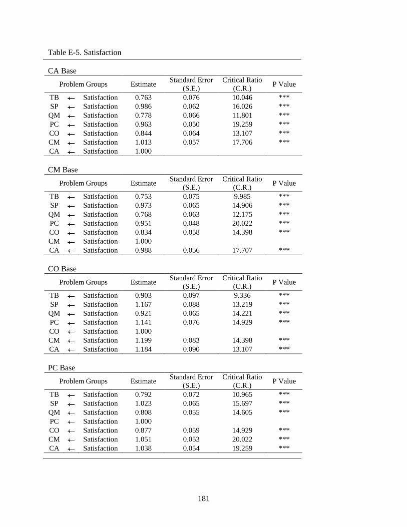
181
Table E-5. Satisfaction
CA Base
Problem Groups Estimate Standard Error
(S.E.)
Critical Ratio
(C.R.) P Value
TB Satisfaction 0.763 0.076 10.046 ***
SP Satisfaction 0.986 0.062 16.026 ***
QM Satisfaction 0.778 0.066 11.801 ***
PC Satisfaction 0.963 0.050 19.259 ***
CO Satisfaction 0.844 0.064 13.107 ***
CM Satisfaction 1.013 0.057 17.706 ***
CA Satisfaction 1.000
CM Base
Problem Groups Estimate Standard Error
(S.E.)
Critical Ratio
(C.R.) P Value
TB Satisfaction 0.753 0.075 9.985 ***
SP Satisfaction 0.973 0.065 14.906 ***
QM Satisfaction 0.768 0.063 12.175 ***
PC Satisfaction 0.951 0.048 20.022 ***
CO Satisfaction 0.834 0.058 14.398 ***
CM Satisfaction 1.000
CA Satisfaction 0.988 0.056 17.707 ***
CO Base
Problem Groups Estimate Standard Error
(S.E.)
Critical Ratio
(C.R.) P Value
TB Satisfaction 0.903 0.097 9.336 ***
SP Satisfaction 1.167 0.088 13.219 ***
QM Satisfaction 0.921 0.065 14.221 ***
PC Satisfaction 1.141 0.076 14.929 ***
CO Satisfaction 1.000
CM Satisfaction 1.199 0.083 14.398 ***
CA Satisfaction 1.184 0.090 13.107 ***
PC Base
Problem Groups Estimate Standard Error
(S.E.)
Critical Ratio
(C.R.) P Value
TB Satisfaction 0.792 0.072 10.965 ***
SP Satisfaction 1.023 0.065 15.697 ***
QM Satisfaction 0.808 0.055 14.605 ***
PC Satisfaction 1.000
CO Satisfaction 0.877 0.059 14.929 ***
CM Satisfaction 1.051 0.053 20.022 ***
CA Satisfaction 1.038 0.054 19.259 ***
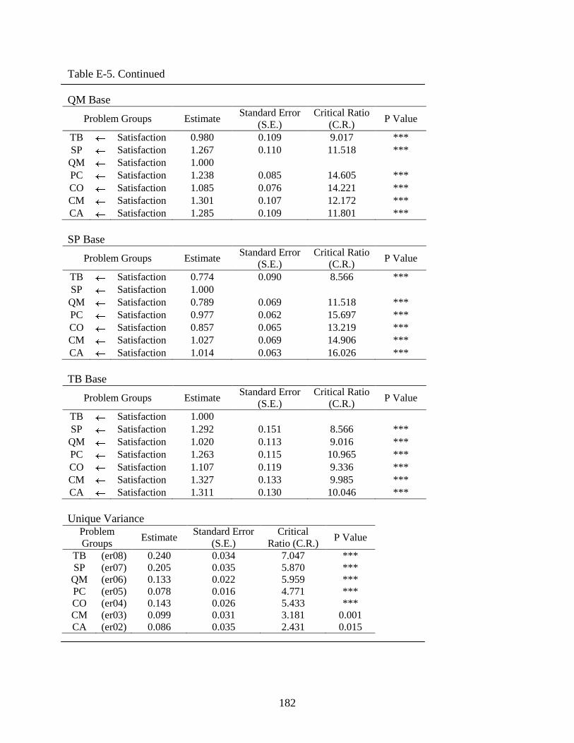
182
Table E-5. Continued
QM Base
Problem Groups Estimate Standard Error
(S.E.)
Critical Ratio
(C.R.) P Value
TB Satisfaction 0.980 0.109 9.017 ***
SP Satisfaction 1.267 0.110 11.518 ***
QM Satisfaction 1.000
PC Satisfaction 1.238 0.085 14.605 ***
CO Satisfaction 1.085 0.076 14.221 ***
CM Satisfaction 1.301 0.107 12.172 ***
CA Satisfaction 1.285 0.109 11.801 ***
SP Base
Problem Groups Estimate Standard Error
(S.E.)
Critical Ratio
(C.R.) P Value
TB Satisfaction 0.774 0.090 8.566 ***
SP Satisfaction 1.000
QM Satisfaction 0.789 0.069 11.518 ***
PC Satisfaction 0.977 0.062 15.697 ***
CO Satisfaction 0.857 0.065 13.219 ***
CM Satisfaction 1.027 0.069 14.906 ***
CA Satisfaction 1.014 0.063 16.026 ***
TB Base
Problem Groups Estimate Standard Error
(S.E.)
Critical Ratio
(C.R.) P Value
TB Satisfaction 1.000
SP Satisfaction 1.292 0.151 8.566 ***
QM Satisfaction 1.020 0.113 9.016 ***
PC Satisfaction 1.263 0.115 10.965 ***
CO Satisfaction 1.107 0.119 9.336 ***
CM Satisfaction 1.327 0.133 9.985 ***
CA Satisfaction 1.311 0.130 10.046 ***
Unique Variance Problem
Groups Estimate
Standard Error
(S.E.)
Critical
Ratio (C.R.) P Value
TB (er08) 0.240 0.034 7.047 ***
SP (er07) 0.205 0.035 5.870 ***
QM (er06) 0.133 0.022 5.959 ***
PC (er05) 0.078 0.016 4.771 ***
CO (er04) 0.143 0.026 5.433 ***
CM (er03) 0.099 0.031 3.181 0.001
CA (er02) 0.086 0.035 2.431 0.015
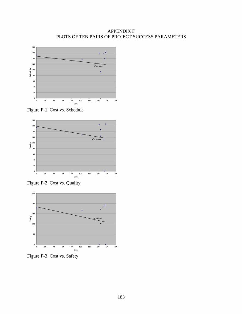
183
APPENDIX F
PLOTS OF TEN PAIRS OF PROJECT SUCCESS PARAMETERS
R2 = 0.0329
0
20
40
60
80
100
120
140
160
180
0 20 40 60 80 100 120 140 160 180
Cost
Sc
he
du
le
Figure F-1. Cost vs. Schedule
R2 = 0.0709
0
20
40
60
80
100
120
140
160
180
0 20 40 60 80 100 120 140 160 180
Cost
Qu
ali
ty
Figure F-2. Cost vs. Quality
R2 = 0.0948
0
50
100
150
200
250
0 20 40 60 80 100 120 140 160 180
Cost
Sa
fety
Figure F-3. Cost vs. Safety
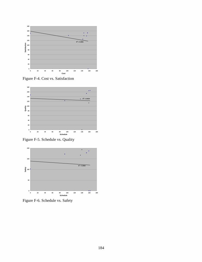
184
R2 = 0.0805
0
20
40
60
80
100
120
140
160
180
0 20 40 60 80 100 120 140 160 180
Cost
Sa
tis
fac
tio
n
Figure F-4. Cost vs. Satisfaction
R2 = 0.0034
0
20
40
60
80
100
120
140
160
180
0 20 40 60 80 100 120 140 160 180
Schedule
Qu
ali
ty
Figure F-5. Schedule vs. Quality
R2 = 0.0063
0
50
100
150
200
0 20 40 60 80 100 120 140 160 180
Schedule
Sa
fety
Figure F-6. Schedule vs. Safety
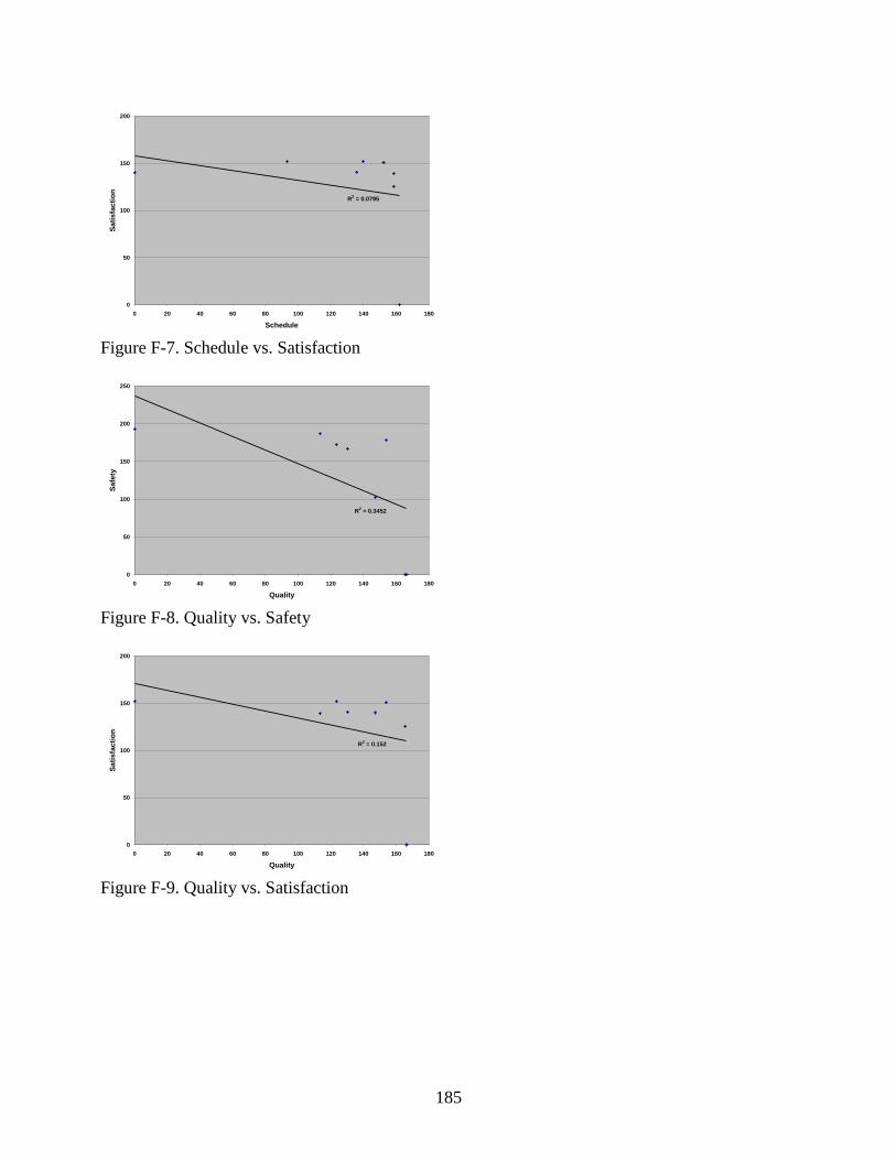
185
R2 = 0.0795
0
50
100
150
200
0 20 40 60 80 100 120 140 160 180
Schedule
Sa
tis
fac
tio
n
Figure F-7. Schedule vs. Satisfaction
R2 = 0.3452
0
50
100
150
200
250
0 20 40 60 80 100 120 140 160 180
Quality
Sa
fety
Figure F-8. Quality vs. Safety
R2 = 0.152
0
50
100
150
200
0 20 40 60 80 100 120 140 160 180
Quality
Sa
tis
fac
tio
n
Figure F-9. Quality vs. Satisfaction
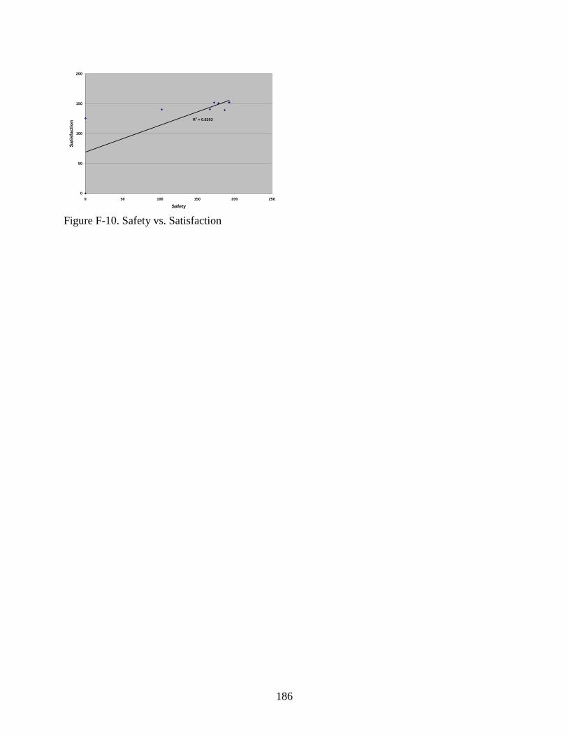
186
R2 = 0.5203
0
50
100
150
200
0 50 100 150 200 250
Safety
Sa
tis
fac
tio
n
Figure F-10. Safety vs. Satisfaction
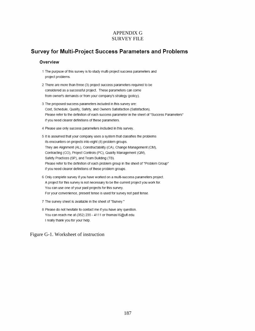
187
APPENDIX G
SURVEY FILE
Figure G-1. Worksheet of instruction
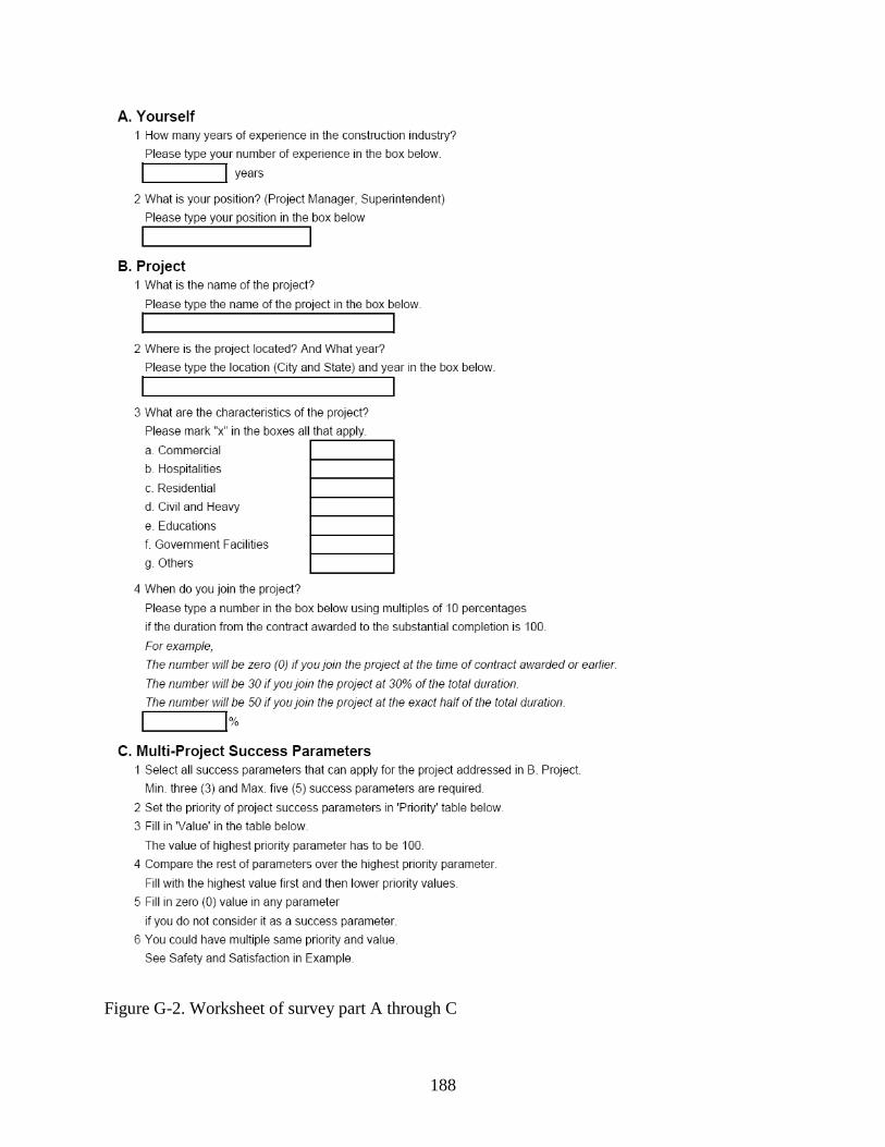
188
Figure G-2. Worksheet of survey part A through C
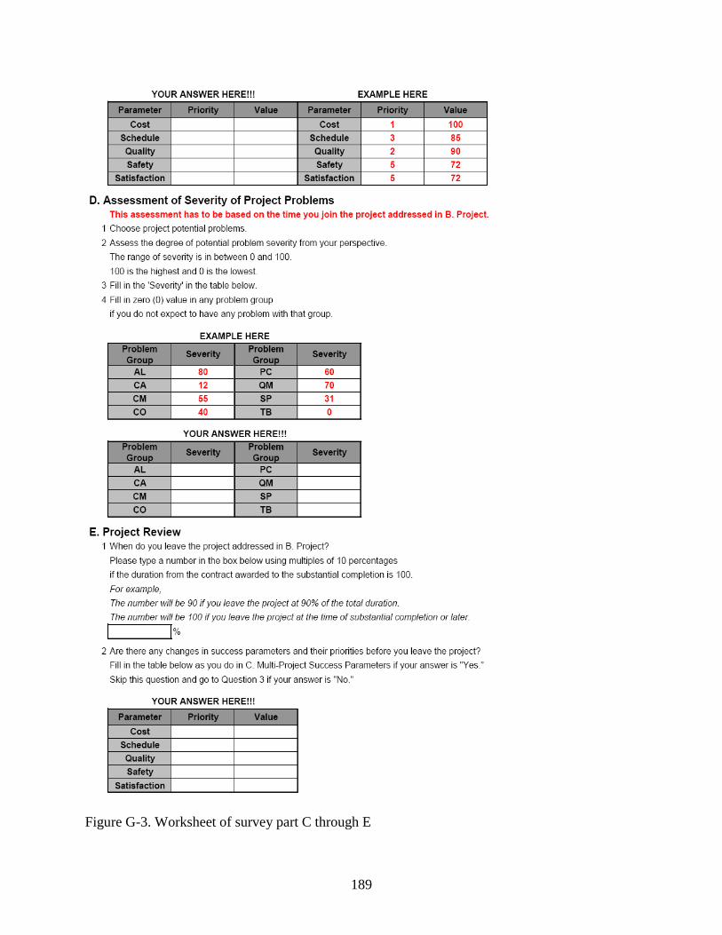
189
Figure G-3. Worksheet of survey part C through E
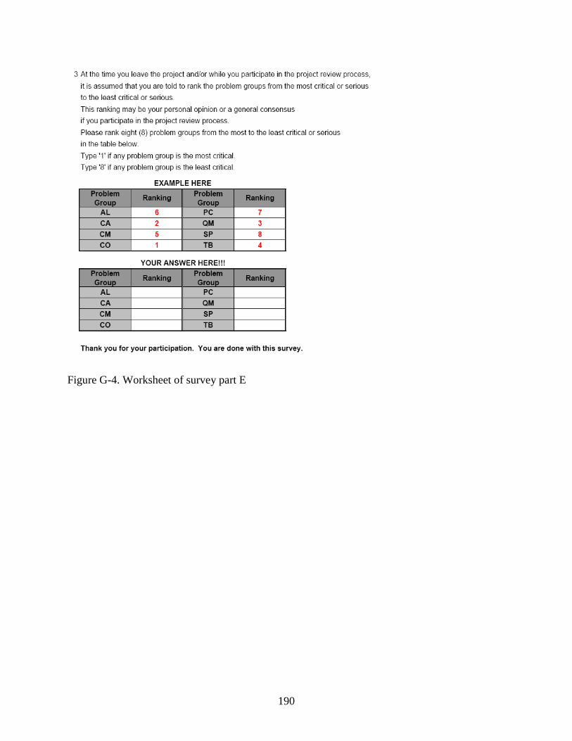
190
Figure G-4. Worksheet of survey part E
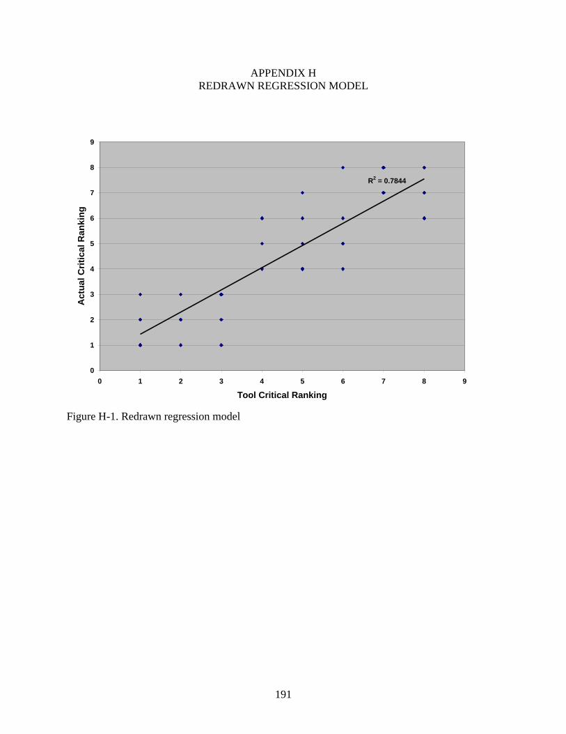
191
APPENDIX H
REDRAWN REGRESSION MODEL
R2 = 0.7844
0
1
2
3
4
5
6
7
8
9
0 1 2 3 4 5 6 7 8 9
Tool Critical Ranking
Ac
tua
l C
riti
ca
l R
an
kin
g
Figure H-1. Redrawn regression model
192
LIST OF REFERENCES
ACITS. (1995). "Factor Analysis Using SAS PROC FACTOR (Stat - 53)."
<http://www.utexas.edu/cc/docs/stat53.html> (Jun. 4, 2009).
Ainsworth, A. (2008). "Canonical Correlation: Equation Psy 524."
<http://www.csun.edu/~ata20315/psy524/docs/Psy524%20Lecture%208%20CC.ppt>
(May 31, 2009).
Bassioni, H. A., Hassan, T. M., and Price, A. D. F. (2008). "Evaluation and analysis of criteria
and sub-criteria of a construction excellence model." Engineering, Construction and
Architectural Management, 15(1), 21-41.
Brown, T. (2006). Confirmatory Factor Analysis for Applied Research, Guilford Press, New
York.
Chan, A. P. C., Scott, D., and Chan, A. P. L. (2004). "Factors Affecting the Success of a
Construction Project." Journal of Construction Engineering and Management, 130(1), 153-
155.
Chan, A. P. C., Scott, D., and Lam, E. W. M. (2002). "Framework of Success Criteria for
Design/Build Projects." Journal of Management in Engineering, 18(3), 120-128.
Cheng, E. W. L. (2001). "SEM being more effective than multiple regression in parsimonious
model testing for management development research." Journal of Management
Development, 20(7), 650-667.
Choi, J., Anderson, S., and Kim, S. J. T. (2006). "Forecasting Potential Risks Through Leading
Indicators to Project Outcome."
Curran, P. J., West, S. G., and Finch, J. F. (1996). "The Robustness of Test Statistics to
Nonnormality and Specification Error in Confirmatory Factor Analysis." Psychological
Methods, 1(1), 16-29.
Dunteman, G. H. (1984). Introduction to Multivariate Analysis, Sage Publications, Beverly Hills.
Edwards, W. (1977). "How to Use Multiattribute Utility Measurement for Social
Decisionmaking." IEEE Transactions on Systems, Man, and Cybernetics, SMC-7(5), 326-
340.
Edwards, W., and Barron, F. H. (1994). "SMARTS and SMARTER: Improved Simple Methods
for Multiattribute Utility Measurement." Organizational Behavior and Human Decision
Processes, 60, 306-325.
Eskildsen, J. K., Kristensen, K., and Juhl, H. J. (2001). "The criterion weights of the EFQM
excellence model." International Journal of Quality & Reliability Management, 18(8), 783-
795.
193
Floyd, F. J., and Widaman, K. F. (1995). "Factor Analysis in the Development and Refinement
of Clinical Assessment Instruments." Psychological Assessment, 7(3), 286-299.
Garson, D. (2008a). "PA 765: Canonical Correlation - Canonical Correlation."
<http://www2.chass.ncsu.edu/garson/pa765/canonic.htm> (Feb. 18, 2008).
Garson, D. (2008b). "Scales and Standard Measures."
<http://faculty.chass.ncsu.edu/garson/PA765/standard.htm> (Jul. 16, 2008).
Garson, D. (2008c). "Structural Equation Modeling: Statnotes."
<http://faculty.chass.ncsu.edu/garson/PA765/structur.htm> (Jul. 7, 2008).
Gibson, E. J., and Dumont, P. (1995). "Project Definition Rating Index (PDRI) for Industrial
Project." Construction Industry Institute (CII) Research Report 113-11.
Griffith, A. F., Gibson, E. J., Tortora, A. L., and Wilson, C. T. (1999). "Project Success Index for
Capital Facility Construction Project." Journal of Performance of Constructed Facilities,
13(1), 39-45.
Hackney, J. W. (1992). Control & Management of Capital Projects - Second Edition, McGraw-
Hills, Inc, New York.
Hair, J. F., Anderson, R. E., Tatham, R. L., and Black, W. (1998). Multivariate Data Analysis,
Prentice-Hall, Englewood, New Jersey.
Herbsman, Z., Chen, W. T., and Epstein, W. C. (1995). "Time Is Money: Innovative Contracting
Methods in Highway Construction." Construction Engineering and Management, 121(3),
273-281.
Herbsman, Z., and Ellis, R. (1992). "Multiparameter Bidding System - Innovation in Contract
Administration." Construction Engineering and Management, 118(1), 142-150.
Kaplan, R. S., and Norton, D. P. (1992). "The Balanced Scorecard - Measures That Drive
Performance." Harvard Business Review, January-February, 71-75.
Ko, H., Cho, C.-H., and Roberts, M. S. (2005). "Internet Uses and Gratifications/A Structural
Equation Model of Interactive Advertising." Journal of Advertising, 34(2), 57-70.
NIST/SEMATECH. (2006). "e-Handbook of Statistical Methods."
<http://www.itl.nist.gov/div898/handbook/eda/section3/eda35b.htm> (Dec. 10, 2008).
Olson, C. L. (1987). Statistics: Making Sense of Data, Allyn and Bacon, Boston.
Oyetunji, A. A. (2001). "Methodology for Selecting Project Delivery and Contracting Strategies
for Capital Projects," Texas A&M University, College Station, TX.
194
Russell, J. S., Jaselskis, E. J., Lawrence, S., Tserng, H.-P., and Prestine, M. (1996).
"Development of a predictive tool for continuous assessment of project performance." The
Construction Industry Institute, The University of Texas Austin, Austin, TX.
Seo, S., Aramaki, T., Hwang, Y., and Hanaki, K. (2004). "Fuzzy Decision-Making Tool for
Environmental Sustainable Buildings." Journal of Construction Engineering and
Management, 130(3), 415-423.
Spector, P. E. (1992). Summated Rating Scale Construction: An Introduction, SAGE
Publications, Newbaury Park, California.
SPSS. (2008). "AMOS."
Thompson, B. (1984). Canonical Correlation Analysis: Uses and Interpretation, Sage
Publications, Beverly Hills.
Thompson, B. (2004). Exploratory and Confirmatory Factor Analysis: Understanding Concepts
and Applications, American Psychological Association, Washington, DC.
Weisstein, E. W. (2009a). "Combination." <http://mathworld.wolfram.com/Combination.html>
(Jun. 14, 2009).
Weisstein, E. W. (2009b). "Variation Coefficient."
<http://mathworld.wolfram.com/VariationCoefficient.html> (Jan. 20, 2009).
Winterfeldt, D., and Edwards, W. (1986). Decision Analysis and Behavioral Research,
Cambridge University Press, Cambridge; New York.
Wynne, J. D. (1982). Learning Statistics: A Common-Sense Approach, Macmillan (New York)
and Collier Macmillan (London), New York and London.
195
BIOGRAPHICAL SKETCH
Seong Jin “Tommy” Kim was born in Seoul, Korea. He has four family members (two
parents and two sisters). He grew up in most his time in Koyansi, Kyunggido. The schools he
has been to are: Shin Do elementary school, Youn Shin middle school, and Dae Shin high school.
Right after he graduated from high school, he went to Soong Sil University for four years of
college, majoring in architectural engineering. During the college years, he joined the army for
two years as other Korean men do. He loved the design of buildings and houses and won a
couple of design competitions during his college years. After graduation he started working with
a general contractor for the next five years, three years in Malaysia and two years in Seoul,
Korea. When he worked for a general contractor in Korea and Malaysia, he had a chance to
meet a lot of people from all over the world and gained experienced in the construction industry.
Even though he loved his job and work, he decided to study more to become a better person in
the construction industry. After five years of work, he continued studying for his master‟s
degree in civil engineering at Texas A&M University. At that time Tommy decided to be a
professor at a university and that is something he would like to do better than anything in the
world. When he was done with his master‟s degree in Texas, he came to the University of
Florida to seek his Ph.D in Design, Construction and Planning. His interests in the construction
industry are project controls and planning with estimating. His specialties are related to cost and
schedule. It has been a long journey to accomplishing his goals but it has still been worth doing.
Tommy likes to cook for his friends and families and loves to see movies. He has been a lecturer
in the department of construction management at East Carolina University since August 2009.