Embed Size (px)
Citation preview
Identifying Bioisosteric Fragments from
Databases of Protein-Ligand Complex X-Ray
Crystallographic Structures
A study submitted in partial fulfilment
of the requirements for the degree of
Master of Science in Chemoinformatics
at
THE UNIVERSITY OF SHEFFIELD
by
LIZ KENNEWELL
September 2004
This project was carried out under the supervision of Dr Claude Luttmann and Dr
Pierre Ducrot, and in conjunction with:
Aventis Pharma
Croix de Berny
20 Avenue Raymond Aron
F-92165 Antony Cedex
France
Table of Contents
1 Abstract ...............................................................................................................1 2 Introduction .........................................................................................................2
2.1 Aims of the project .......................................................................................2 2.2 Outline of the report .....................................................................................3 2.3 Acknowledgments ........................................................................................4
3 Background .........................................................................................................5 3.1 Bioisosterism................................................................................................5
3.1.1 Bioisosteric replacement.......................................................................5 3.1.2 Types of bioisosteric replacements.......................................................7 3.1.3 Examples of bioisosteric replacements in drug design .........................8
3.2 Protein-ligand binding ................................................................................12 3.2.1 Hydrogen bonds (H-bonds).................................................................12 3.2.2 Ionic bonds .........................................................................................13 3.2.3 Van der Waals interactions .................................................................14 3.2.4 Ion- dipole and dipole-dipole interactions ...........................................14 3.2.5 Hydrophobic interactions ....................................................................14
3.3 Databases..................................................................................................14 3.3.1 Protein Data Bank (PDB) ....................................................................15 3.3.2 Cambridge Structural Database (CSD)...............................................16 3.3.3 IsoStar ................................................................................................16 3.3.4 SuperStar database............................................................................20 3.3.5 BIOSTER database ............................................................................20 3.3.6 ReliBase+ ...........................................................................................21
3.4 Calculating similarities between functional groups.....................................21 3.5 Identifying common chemical replacements in drug-like compounds ........23 3.6 Conclusion .................................................................................................24
4 Methodology......................................................................................................25 4.1 Overall methodology ..................................................................................25 4.2 Software and programming languages used .............................................26
4.2.1 MOE....................................................................................................26 4.2.2 Scientific Vector Language (SVL) .......................................................26
4.3 Ligand Dataset ...........................................................................................27 4.4 Splitting the ligands into fragments ............................................................28
4.4.1 Splitting Molecule function ..................................................................28
4.5 Identifying fragment pairs...........................................................................33 4.5.1 Scoring overlap...................................................................................34 4.5.2 Comparing the molecules and scoring the overlap.............................37 4.5.3 Defining bioisosteric fragments...........................................................42 4.5.4 Scoring function description................................................................47 4.5.5 Development and modifications of the function ..................................51 4.5.6 Adding attachment points ...................................................................55 4.5.7 Results database structure .................................................................55 4.5.8 Limitations with the scoring function ...................................................56
5 Results ..............................................................................................................61 5.1 cdk2 ligand dataset ....................................................................................63 5.2 cdk4 ligand dataset ....................................................................................64 5.3 Factor Xa ligand dataset ............................................................................65
6 Conclusions.......................................................................................................66
1 Abstract
Bioisosteres are defined as functional groups or atoms that are structurally
different but can form similar intermolecular interactions therefore still retaining
biological activity. Bioisosteres have an important role in the lead generation or
optimisation stages of drug design as bioisosteric replacements can be utilised to
address issues such as solubility, ADME and toxicity problems. The aim of this
project is to identify potential bioisosteres that exist within a set of aligned ligands for
a particular protein target. Rather than determining potential bioisosteric fragments
via observed activity data, this project will aim to identify possible bioisosteric
fragments via structural data. All the ligands within one dataset bind to the same
protein thus ensuring they all have similar activity for the same target.
A function was written in SVL (Scientific Vector Language), as the function will
run using the MOE software, to automate this process. Pairs of ligands, extracted
from the same dataset, are compared to each other to identify fragments within the
ligands which occupy a similar space within the ligand. The fragments are identified
by comparing the volume overlap between the two ligands. Fragments with a high
degree of overlap will occupy a similar position within the protein’s active site and
hence are assumed to have a similar role within the ligand. The fragments do not
necessarily have to be involved in intermolecular binding but can play other
important roles such as linker or scaffold roles.
The concept of identifying potential bioisosteres via structural data has been
shown to work as fragment pairs that occupy the same space within a pair of aligned
ligands have been identified. The function developed within this project can be
applied to sets of different ligands and can be run against both external and internal
ligand datasets. These identified bioisosteric fragments would then be investigated
further to determine whether they can be used to improve the properties of a lead
compound.
1
2 Introduction
The following thesis describes the development of a method for identifying
potential bioisosteric fragments within a set of ligands specific to a particular protein
target. Bioisosteres have been defined as
“Functional groups or atoms that are structurally different but can form similar
intermolecular interactions hence still retaining biological activity.” (Watson et al. 2001)
As bioisosteres do not change the biological activity of ligands they have an
important role in the lead generation or optimisation stage of drug design.
Bioisosteric replacements can be utilised to address issues such as solubility,
ADME and toxicity problems.
2.1 Aims of the project
The aim of this project is to identify potential bioisosteres that exist within a set
of ligands for a particular protein target. Rather than determining potential
bioisosteric fragments via observed activity data, this project will aim to identify
possible bioisosteric fragments via structural data. All the ligands bind to the same
protein thus ensuring they all have similar activity for the same target. The identified
potential bioisosteres may have different roles within the ligand and may not
necessarily be directly involved intermolecular bonding. These roles may include:
o Be part of a linker group which makes no interaction with the protein
but ensures the functional groups are in the right orientation to make
the correct intermolecular contacts.
o Be part of the scaffold maintaining the structure of the ligand.
o Be a functional group involved in forming intermolecular interactions
with the protein.
Identifying potential bioisosteres within other regions could be important as
they may have an impact on other properties without having a detrimental effect on
the binding affinity (as they are not involved in making intermolecular bonds).
The identified fragment pairs are only bioisosteric if they can be interchanged
2

within the ligands whilst maintaining a similar biological activity. As all the ligands,
within a dataset, bind to the same protein target, it is assumed that they have the
similar biological activity. The degree of activity between the ligands may vary even
when the ligands are exerting a similar effect. Although the ligands have the same
biological activity, they may differ in terms of other physiochemical properties, such
as solubility, ADME (absorption, distribution, metabolism, excretion) or toxicity.
Replacement of one bioisostere for another may alter one or more of these
properties.
Potential bioisosteres will be identified based on structural comparisons
between ligands. Additional work would then need to be undertaken to verify
whether which, if any, properties of the ligand the bioisosteric replacement alters.
This will determine whether the identified bioisosteric replacement could be
potentially useful at a lead generation or lead optimisation stage. It is only
worthwhile incorporating a bioisosteric replacement into a lead compound if it
produces a desirable effect e.g. reduces the compound’s toxicity.
All the ligands, within the same dataset, bind to the same protein target so the
identified bioisosteres will be specific to a particular target protein. The developed
methodology can be applied to any protein target and its ligands. It may be possible
to extrapolate the resulting bioisosteres to proteins within the same class but there is
no reason to believe that this will be possible across different protein classes.
However, it may be the case that identical, or similar, bioisosteric pairs emerge for
different protein classes. If this occurs then it may be possible to make more
general observations.
2.2 Outline of the report
The following thesis outlines the development of a function to identify potential
bioisosteres.
The following chapter is a review of the current literature in this field and
provides background information to the subject area. It details the concept behind
bioisosterism and its role in the drug discovery process along with some examples.
This should help explain the rationale for conducting this project. The chapter also
describes some of the databases currently available which aim to assist in the
3

identification of bioisosteres.
The Methodology chapter describes in detail the development of a function
which was designed to identify potential bioisosteric fragments. This section
includes explanations of how the ligands were compared in order to identify any
potential bioisosteres existing between them and also the criteria used to define the
fragment pairs.
The Results chapter of the report shows some examples of the fragment pairs
identified from publicly available protein databases. The function was also run on
internal protein-ligand databases but due to confidentiality reasons, these results are
not shown within this report.
Finally the conclusions drawn from the project are discussed along with how
the developed function can be taken forward.
2.3 Acknowledgments
This project was carried out in conjunction with Aventis Pharma, Paris. I would
like to thank the Chemoinformatics team at Aventis for all their help during my time
there. I would especially like to thank Dr Pierre Ducrot and Dr Claude Luttmann, my
supervisors whilst at Aventis, for all their help, ideas and advice.
I would also like to thank Prof Peter Willet, my Sheffield supervisor, for his
advice and guidance given whilst undertaking this dissertation.
4
3 Background
The following chapter describes the background to the subject area and
details the concept behind bioisosterism. It highlights the important role of
bioisosterism within the drug discovery process, along with some examples, and
hence the rationale for carrying out the following project. There is also a review of
some studies which have looked at methods for identifying bioisosteres. There is
also a description of the currently available databases which aim to assist in the
identification of bioisosteres.
3.1 Bioisosterism
Friedman introduced the concept of bioisosterism in 1951 and defined
bioisosteres as molecules or functional groups which have similar chemical and
physical properties and hence similar biological activity (Watson et al. 2001).
Since then, the growth of crystallographic data has lead to a greater
understanding of the nature of intermolecular interactions between molecules (e.g.
proteins and their ligands). This has lead to the bioisostere definition being
extended to include functional groups or atoms that are structurally different but can
form similar intermolecular interactions but again still retaining biological activity.
(Watson et al. 2001).
3.1.1 Bioisosteric replacement
The concept of bioisosterism is an important approach in drug design as it is
envisaged that functional groups within a lead compound may be interchanged with
a bioisosteric functional group and still preserve biological activity. The rationale
being that the modified compound could possess more desirable chemical or
physical properties than the original molecule while retaining biological activity
against the same target (Patani & LaVoie 1996). Therefore during the lead
optimisation stage, bioisosteric replacements can be used in an attempt to optimise
desirable properties or minimise adverse ones. In order to retain biological activity,
bioisosteric groups must also be similar in some important physical property e.g.
size, ability to form intermolecular interactions.
5
Conducting bioisosteric replacements will alter one or more properties of the
molecule such as size, partition coefficient (logP), logD, pKa, reactivity, solubility,
metabolism or binding properties whilst maintaining biological activity. Different
bioisosteric replacements will lead to varying alterations in the molecule’s properties
depending on what role the modified group has within the molecule. The degree to
which the property is changed, which could be an improvement or reduction, will
also vary between bioisosteric replacements.
A modified group may have one, or several, roles within a molecule including
(Vyvyan 2004):
- structural role – e.g. as a linker group ensuring the functional groups
within a molecule are positioned correctly to make the necessary
intermolecular interactions.
- receptor interactions – e.g. forming non-bonded interactions with a
protein target
- pharmacokinetic role – e.g. affecting the logP and logD value
- metabolism – affecting the metabolism of the molecule and hence
possibly affecting its duration of activity
- toxicity – affecting the toxicity of the molecule
A bioisosteric replacement may affect more than one property of the molecule
which could be advantageous in the lead optimisation stage.
Bioisosteric replacement could take place within scaffold regions of molecules.
Scaffold regions within a ligand position the substituents so they can make
favourable interactions with residues in a protein binding site (Bohl et al. 2002). Any
replacements within a scaffold region must ensure that the relevant substituents can
be positioned correctly to form the appropriate intermolecular bonds.
Developing novel compounds with drug-like features which are also patentable
is becoming increasing challenging especially for extensively researched and
validated drug targets (Showell & Mills 2003). As the number of me-too compounds
increases, the issue of discovering novel compounds will become even more
important. Bioisosteric replacements may help to discover new classes of
6
compounds with no current patent coverage which is an obvious benefit in the drug
design process.
3.1.2 Types of bioisosteric replacements
Bioisosteres can be classified as either classical or nonclassical (Patani &
LaVoie 1996). Classical bioisosteres are defined using Grimm’s Hydride
Displacement Law in which the bioisosteric groups have the same number of
valance electrons and Erlenmeyer’s definition in which the atoms, ions or molecules
have identical peripheral layers of electrons (Patani & LaVoie 1996, Vyvyan 2004).
The classical bioisostere group is commonly divided into several discrete
categories – monovalent atoms or groups, divalent atoms or groups, trivalent atoms
or groups, tetrasubstituted atoms and ring equivalents (Patani & LaVoie 1996).
Chlorine is used as bioisosteric replacement for hydrogen or methyl groups as
it can alter a molecule’s metabolism. In the case of Phenobarbital, replacement of
the hydrogen at the para position with chlorine prevents its metabolism to a
glucuronide conjugate. The substituted chlorine atom blocks the Phenobarbital’s
metabolism hence increasing its duration of action (Patani & LaVoie 1996).
The other major group of bioisosteres are classified as non-classical. They
differ from classical bioisosteres, in that they do not have the same number of
atoms, steric or valence electrons but produce a similar biological activity. Non-
classical bioisosteres retain the spatial arrangement, electronic properties or some
other physiochemical property that is crucial in retaining biological activity (Patani &
LaVoie 1996). The growth in the number of molecules and protein-ligand
complexes whose structures have been determined by crystallographic techniques
has assisted in the identification of nonclassical bioisosteres.
As with classical bioisosteres, non-classical bioisosteres can be subdivided
into groups: rings versus noncyclic structures and exchangeable groups.
7
3.1.3 Examples of bioisosteric replacements in drug design
The previous section has described the theory behind bioisosterism and how it
can be a powerful tool for medicinal chemists when developing novel compounds.
The following section describes just a few examples of where bioisosterism has
been utilised in the drug design process to provide leads for improving existing
compounds.
3.1.3.1 Bioisosteres of endothelin antagonists
Endothelins are potent endogenous peptide vasoconstrictors and mitogens.
Research has looked into the development of endothelin receptor antagonists which
could potentially help to treat diseases with a significant vasoconstrictive or
proliferative component. Many antagonists have been discovered which are
structurally diverse and have varying degrees of potency and subtype selectivity
(Mederski et al. 1998). One similarity between the majority of the determined
structures that have been identified is that they all contain a methylendioxyphenyl
group: a group commonly found in medicinal compounds.
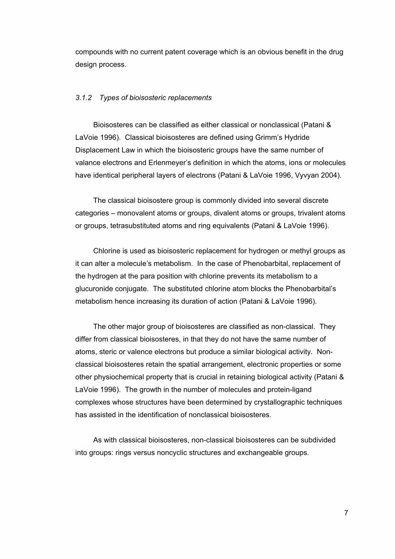
Mederski et al. (1998) tested a previous hypothesis which stated that a
benzothiadiazole group was a suitable bioisostere for the methylendioxyphenyl
group (see Figure 3.1-1 for structure diagrams of these groups). This bioisostere
was identified, in a previous study, through comparing physicochemical properties
using a Kohonen neural network. The current study looked at six structures, and
created six new molecules in which a methylendioxyphenyl group was replaced with
a benzodioxole or a benzothiadiazole group (see Figure 3.1-2 below). The twelve
structures were then tested for their ability to specifically inhibit binding to several
receptor sites. The results showed that the benzothiadiazole derivatives showed
improved binding affinities for one of the receptors tested.
Figure 3.1-1 – methylendioxyphenyl and benzothiadiazole groups
8
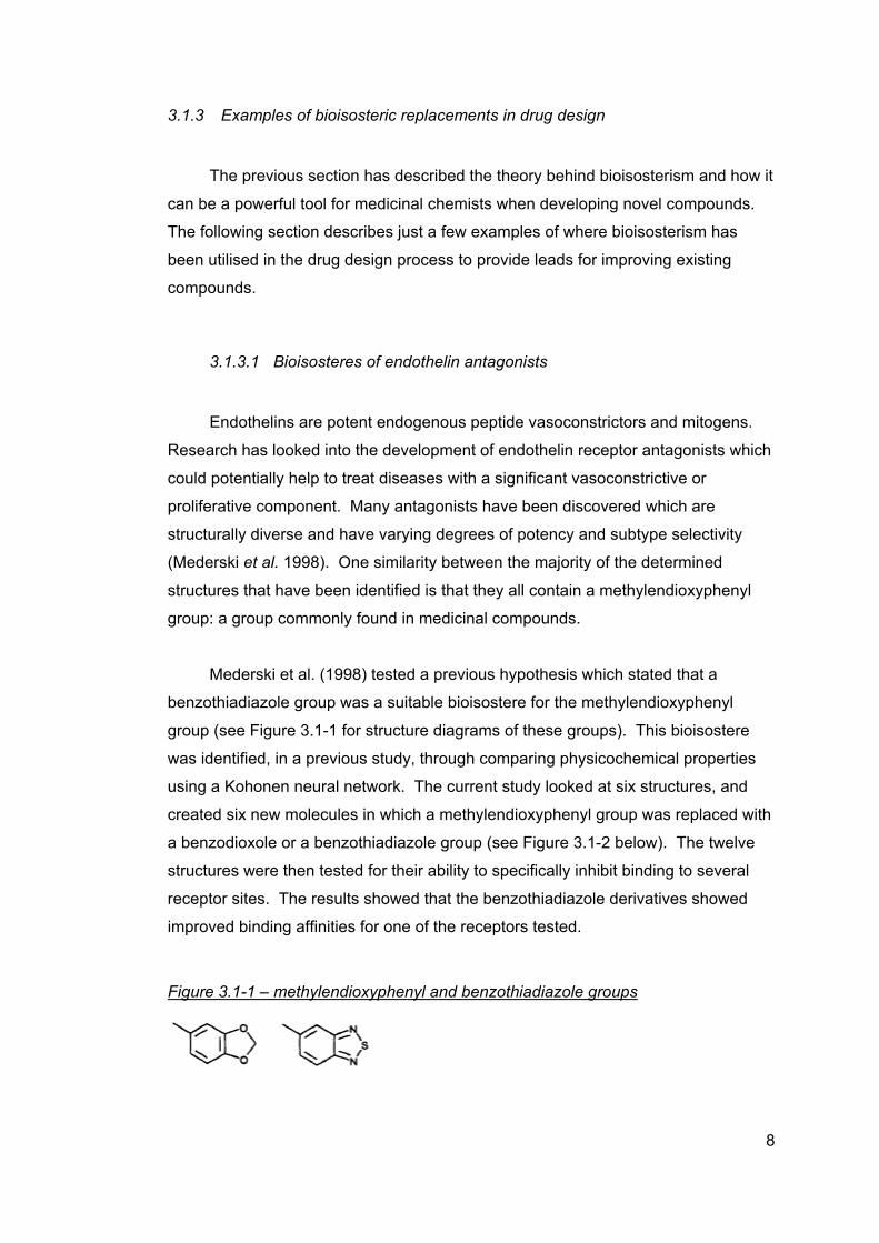
Figure 3.1-2 – Compounds tested – for each compound the R group was replaced
with a methylendioxyphenyl group and then a benzothiadiazole group
The study concluded that a benzothiadiazole group might be a bioisoster of
methylendioxyphenyl group when looking at endothelin receptor antagonists. The
authors argue that benzothiadiazole has a more pronounced electron withdrawing
character than methylendioxyphenyl and hence leads to differences in binding
affinity (in this case improvement). These findings could be used to help develop
novel endothelin receptor antagonists with more potent binding affinity and hence
greater efficacy.
As methylendioxyphenyl groups are common in medicinal compounds, could
this bioisosteric replacement be advantageous in other drug compounds?
3.1.3.2 Silicon isosteres
Showell & Mills (2003) looked at the less common replacement of silicon for a
fully substituted sp3 carbon. In 2001, less than 1% of patent applications related to
compounds containing phosphorous, silicon and other less common elements in the
drug discovery field (Showell & Mills 2003). Although both carbon and silicon
9
contain four valence electrons, the two elements differ significantly in a number of
physiochemical properties, an example being the difference in molecular size and
shape. Silicon-containing bonds are always longer than equivalent carbon-
containing bonds. This difference leads to changes in the size and shape of silicon
containing compounds compared to equivalent carbon containing compounds.
These changes could potentially alter the nature of the interactions (and hence
potential biological activity) a silicon-containing compounds makes with a target
protein compared to the analogous carbon-containing molecule. Even though the
silicon containing compounds are likely to be larger this could enhance ligand
binding.
As well as the potential for improving biological activity, the study also
highlighted some potential limitations, such as increased lipophilicity and concerns
regarding toxicity of silicon-containing compounds. The authors present research
which suggests, contrary to popular opinion, that there is no systematic toxic liability
with silicon in chemically stable molecules. There are currently no silicon-containing
drugs approved in the US or Europe but the authors conclude that introducing
silicon isosteres at the lead optimisation stage could generate several advantages
such as altered efficacy, improved selectivity and, importantly, patentability of the
molecule.
3.1.3.3 Bioisosteric replacements in celecoxib
The following example shows how bioisosteric replacements can be utilised
within an identified pharmacophore to enhance binding affinity of a compound.
When launched, Celecoxib (Celebrex) provided significant benefits for the treatment
of rheumatoid arthritis and osteoarthritis over previously available non-steroidal anti-
inflammatory drugs (NSAIDs) (see Figure 3.1-3 for the structure of celecoxib).
Celecoxib’s main advantage lies in its ability to selectively inhibit the enzyme,
cyylooxygenase (COX-2) rather than both COX-1 and COX-2 as is the case with
traditional NSAIDs. This selectivity leads to an improved side-effect profile for
celecoxib especially regarding gastrointestinal toxicity.
10
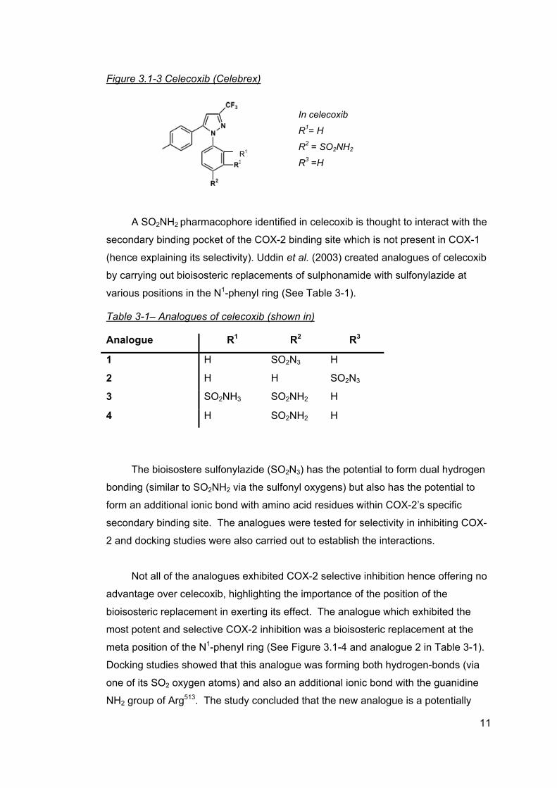
Figure 3.1-3 Celecoxib (Celebrex)
In celecoxib
R1= H
R2 = SO2NH2
R3 =H R1
A SO2NH2 pharmacophore identified in celecoxib is thought to interact with the
secondary binding pocket of the COX-2 binding site which is not present in COX-1
(hence explaining its selectivity). Uddin et al. (2003) created analogues of celecoxib
by carrying out bioisosteric replacements of sulphonamide with sulfonylazide at
various positions in the N1-phenyl ring (See Table 3-1).
Table 3-1– Analogues of celecoxib (shown in)
Analogue R1 R2 R3
1 H SO2N3 H
2 H H SO2N3
3 SO2NH3 SO2NH2 H
4 H SO2NH2 H
The bioisostere sulfonylazide (SO2N3) has the potential to form dual hydrogen
bonding (similar to SO2NH2 via the sulfonyl oxygens) but also has the potential to
form an additional ionic bond with amino acid residues within COX-2’s specific
secondary binding site. The analogues were tested for selectivity in inhibiting COX-
2 and docking studies were also carried out to establish the interactions.
Not all of the analogues exhibited COX-2 selective inhibition hence offering no
advantage over celecoxib, highlighting the importance of the position of the
bioisosteric replacement in exerting its effect. The analogue which exhibited the
most potent and selective COX-2 inhibition was a bioisosteric replacement at the
meta position of the N1-phenyl ring (See Figure 3.1-4 and analogue 2 in Table 3-1).
Docking studies showed that this analogue was forming both hydrogen-bonds (via
one of its SO2 oxygen atoms) and also an additional ionic bond with the guanidine
NH2 group of Arg513. The study concluded that the new analogue is a potentially
11
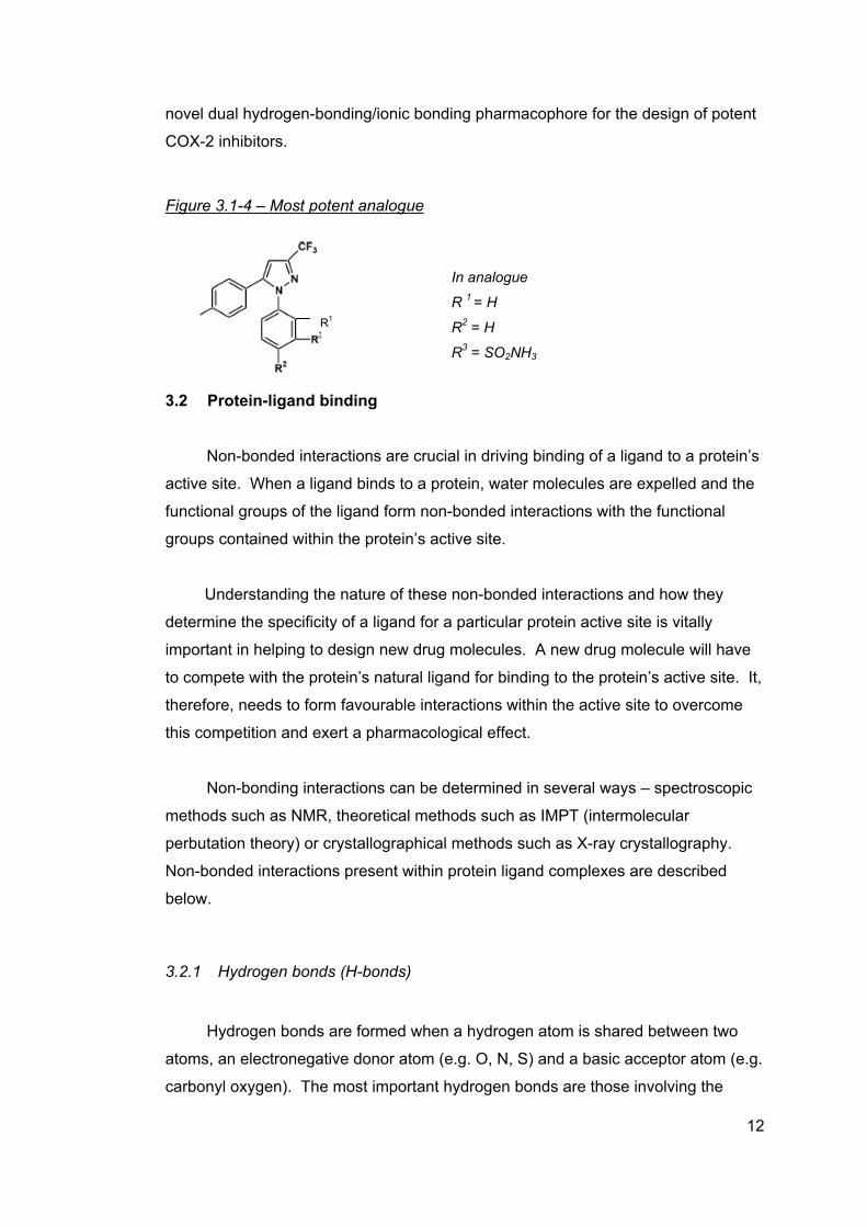
novel dual hydrogen-bonding/ionic bonding pharmacophore for the design of potent
COX-2 inhibitors.
Figure 3.1-4 – Most potent analogue
In analogue
R 1 = H
R2 = H
R3 = SO2NH3
R1
3.2 Protein-ligand binding
Non-bonded interactions are crucial in driving binding of a ligand to a protein’s
active site. When a ligand binds to a protein, water molecules are expelled and the
functional groups of the ligand form non-bonded interactions with the functional
groups contained within the protein’s active site.
Understanding the nature of these non-bonded interactions and how they
determine the specificity of a ligand for a particular protein active site is vitally
important in helping to design new drug molecules. A new drug molecule will have
to compete with the protein’s natural ligand for binding to the protein’s active site. It,
therefore, needs to form favourable interactions within the active site to overcome
this competition and exert a pharmacological effect.
Non-bonding interactions can be determined in several ways – spectroscopic
methods such as NMR, theoretical methods such as IMPT (intermolecular
perbutation theory) or crystallographical methods such as X-ray crystallography.
Non-bonded interactions present within protein ligand complexes are described
below.
3.2.1 Hydrogen bonds (H-bonds)
Hydrogen bonds are formed when a hydrogen atom is shared between two
atoms, an electronegative donor atom (e.g. O, N, S) and a basic acceptor atom (e.g.
carbonyl oxygen). The most important hydrogen bonds are those involving the
12
oxygen and nitrogen atoms of the carboxyl, hydroxyl, carbonyl, amino, imino and
amido groups. These bonds are responsible for maintaining the tertiary structure of
proteins and nucleic acids, as well as the binding of many drugs (Andrews &
Tintelnot 1990). In proteins, most hydrogen donor and acceptor groups are found in
the peptide backbone.
Different hydrogen bonds have different lengths and energies depending on
the nature of the donor and acceptor atoms (Stryer 1988). Hydrogen bonds are
stronger than van der Waals bonds but are much weaker than covalent bonds.
Hydrogen bonds are highly directional and are thought to be responsible for the
specificity of receptor sites. The strongest hydrogen bonds are formed when the
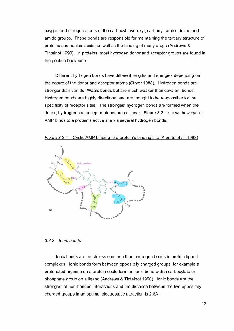
donor, hydrogen and acceptor atoms are collinear. Figure 3.2-1 shows how cyclic
AMP binds to a protein’s active site via several hydrogen bonds.
Figure 3.2-1 – Cyclic AMP binding to a protein’s binding site (Alberts et al. 1998)
3.2.2 Ionic bonds
Ionic bonds are much less common than hydrogen bonds in protein-ligand
complexes. Ionic bonds form between oppositely charged groups, for example a
protonated arginine on a protein could form an ionic bond with a carboxylate or
phosphate group on a ligand (Andrews & Tintelnot 1990). Ionic bonds are the
strongest of non-bonded interactions and the distance between the two oppositely
charged groups in an optimal electrostatic attraction is 2.8Å.
13
3.2.3 Van der Waals interactions
The basis of a van der Waals interaction is that the distribution of electronic
density around atoms changes over time. An asymmetrical electronic density
around one atom encourages a similar asymmetry in the electronic density in a
neighbouring atom. The resulting attraction between a pair of atoms increases as
they get closer until it reaches a maximum when they are separated by the van der
Waals contact distance (Stryer 1987).
van der Waals interactions are weaker than hydrogen and ionic bonds. These
interactions only become significant when numerous atoms in one of a pair of
molecules can simultaneously come close to many atoms of the other molecule
(which can be the case when a ligand binds to a protein) (Stryer 1987).
3.2.4 Ion- dipole and dipole-dipole interactions
These interactions are formed when permanent dipoles interact favourably
with other permanent dipoles or ions. A partial negative charge on one molecule is
electrostatically attracted to the partial negative charge on another molecule. The
most common dipole in proteins is formed by the amide linkage.
3.2.5 Hydrophobic interactions
Another important effect which should be taken into consideration when
analysing protein-ligand interactions is hydrophobic interactions. Hydrophobic
interactions are formed when a ligand and a protein approach each other and water
is extruded from the space between them. These interactions are entropy driven, if
expelling water results in an increase in entropy then there is a resulting decrease in
energy. These interactions are particularly important in non-covalent intermolecular
interactions in aqueous solution (Andrews & Tintelnot 1990).
3.3 Databases
Several databases exist which contain information regarding intermolecular
14

interactions. This information can be used to gain an understanding of the nature of
these interactions and how they can be manipulated in order to develop novel drug
compounds. They can also be used to help identify potential bioisosteres within
ligands.
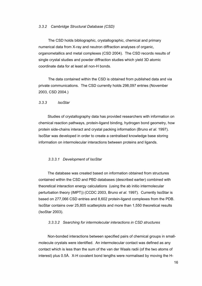
3.3.1 Protein Data Bank (PDB)
The Protein Data Bank (PDB) was established in 1971 by the Brookhaven
National Laboratories and is an archive of structural data for biological
macromolecules (Berman et al. 2000). The vast majority (~90%) of the structures
depict protein, viruses or peptide molecules with the remaining structures being
nucleic acid, protein/nucleic acid complexes or carbohydrate molecules. Figure
3.3-1 shows an example of PBD entry.
Figure 3.3-1 - Four PBD entries showing HIV-1 Protease enzyme (shown as an α-
carbon chain) bound with four drugs(shown as spacefilling models) : Indinavir (PDB
entry ), Saquinavir (PDB entry ), Ritonavir (PDB entry ), and 1hsg 1hxb 1hxw
Nelfinavir (PDB entry ) (PBD 2000).1ohr
The PDB currently contains 25,251 structures (as of 27 April 2004) of which
3731 structures have been determined by Nuclear Magnetic Resonance and 21,520
structures by X-ray diffraction or other methods (RCSG PDB 2004). It is estimated
that the PDB will grow to more than 35,000 structures by 2005 due to an increasing
interest in structural proteomics (Hendlich et al. 2003).
15
3.3.2 Cambridge Structural Database (CSD)
The CSD holds bibliographic, crystallographic, chemical and primary
numerical data from X-ray and neutron diffraction analyses of organic,
organometallics and metal complexes (CSD 2004). The CSD records results of
single crystal studies and powder diffraction studies which yield 3D atomic
coordinate data for at least all non-H bonds.
The data contained within the CSD is obtained from published data and via
private communications. The CSD currently holds 298,097 entries (November
2003, CSD 2004.)
3.3.3 IsoStar
Studies of crystallography data has provided researchers with information on
chemical reaction pathways, protein-ligand binding, hydrogen bond geometry, how
protein side-chains interact and crystal packing information (Bruno et al. 1997).
IsoStar was developed in order to create a centralised knowledge base storing
information on intermolecular interactions between proteins and ligands.
3.3.3.1 Development of IsoStar
The database was created based on information obtained from structures
contained within the CSD and PBD databases (described earlier) combined with
theoretical interaction energy calculations (using the ab initio intermolecular
perturbation theory (IMPT)) (CCDC 2003, Bruno et al. 1997). Currently IsoStar is
based on 277,066 CSD entries and 8,602 protein-ligand complexes from the PDB.
IsoStar contains over 25,805 scatterplots and more than 1,550 theoretical results
(IsoStar 2003).
3.3.3.2 Searching for intermolecular interactions in CSD structures
Non-bonded interactions between specified pairs of chemical groups in small-
molecule crystals were identified. An intermolecular contact was defined as any
contact which is less than the sum of the van der Waals radii (of the two atoms of
interest) plus 0.5Å. X-H covalent bond lengths were normalised by moving the H-
16
atom along the observed X-H vector until the X-H distance is equal to a standard
value (Bruno et al. 1997).
3.3.3.3 Searching for intermolecular interactions in PBD structures
X-ray crystallography structures of protein-ligand complexes at less than 2.5Å
resolution were searched to identify protein-ligand interactions. A ligand is defined
as a peptide of up to 10 residues long or a non-peptide molecule of at least 9 atoms.
Complexes containing DNA or RNA or structures marked ‘mutated’ were excluded
from the search (Bruno et al. 1997).
SYBYL software was used to extract the ligand from the complex along with
any protein residues, water molecules and other chemical entities within 4Å of any
ligand atom. Searches were then performed to identify non-bonded contacts
between:
- protein residues and ligand molecules
- water and ligand molecules
- water and protein residues
3.3.3.4 Scatterplots and contour maps
Scatterplots show the distribution of contact groups around a central group. A
scatterplot is produced by choosing a central group and searching the CSD or PBD
for all the molecules which contain this central group. The central groups are
overlaid and the position of the contact group is marked. Once all the central groups
have been overlaid, a scatterplot is produced which shows all the possible positions
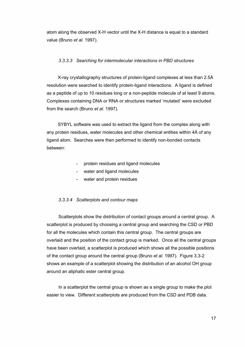
of the contact group around the central group (Bruno et al. 1997). Figure 3.3-2
shows an example of a scatterplot showing the distribution of an alcohol OH group
around an aliphatic ester central group.
In a scatterplot the central group is shown as a single group to make the plot
easier to view. Different scatterplots are produced from the CSD and PDB data.
17
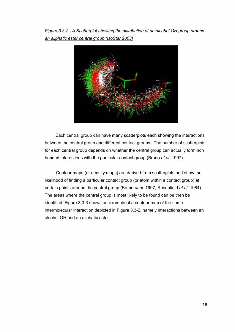
Figure 3.3-2 - A Scatterplot showing the distribution of an alcohol OH group around
an aliphatic ester central group (IsoStar 2003)
Each central group can have many scatterplots each showing the interactions
between the central group and different contact groups. The number of scatterplots
for each central group depends on whether the central group can actually form non
bonded interactions with the particular contact group (Bruno et al. 1997).
Contour maps (or density maps) are derived from scatterplots and show the
likelihood of finding a particular contact group (or atom within a contact group) at
certain points around the central group (Bruno et al. 1997, Rosenfield et al. 1984).
The areas where the central group is most likely to be found can be then be
identified. Figure 3.3-3 shows an example of a contour map of the same
intermolecular interaction depicted in Figure 3.3-2, namely interactions between an
alcohol OH and an aliphatic ester.
18
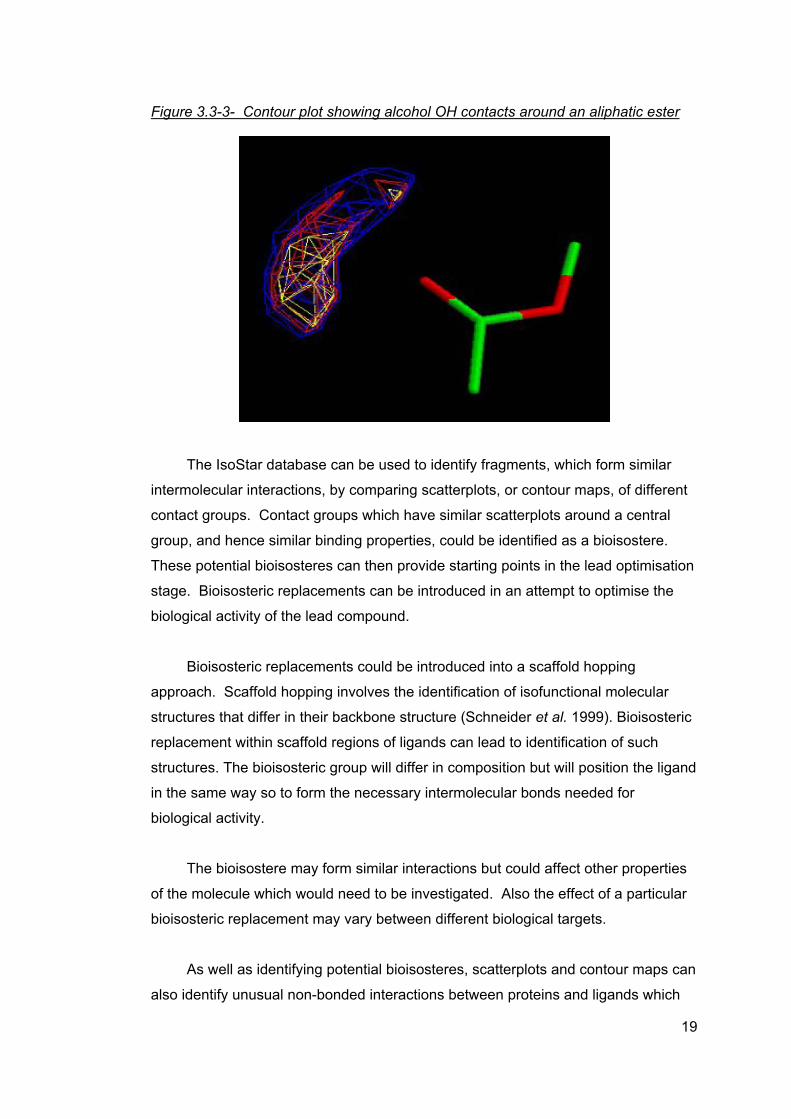
Figure 3.3-3- Contour plot showing alcohol OH contacts around an aliphatic ester
The IsoStar database can be used to identify fragments, which form similar
intermolecular interactions, by comparing scatterplots, or contour maps, of different
contact groups. Contact groups which have similar scatterplots around a central
group, and hence similar binding properties, could be identified as a bioisostere.
These potential bioisosteres can then provide starting points in the lead optimisation
stage. Bioisosteric replacements can be introduced in an attempt to optimise the
biological activity of the lead compound.
Bioisosteric replacements could be introduced into a scaffold hopping
approach. Scaffold hopping involves the identification of isofunctional molecular
structures that differ in their backbone structure (Schneider et al. 1999). Bioisosteric
replacement within scaffold regions of ligands can lead to identification of such
structures. The bioisosteric group will differ in composition but will position the ligand
in the same way so to form the necessary intermolecular bonds needed for
biological activity.
The bioisostere may form similar interactions but could affect other properties
of the molecule which would need to be investigated. Also the effect of a particular
bioisosteric replacement may vary between different biological targets.
As well as identifying potential bioisosteres, scatterplots and contour maps can
also identify unusual non-bonded interactions between proteins and ligands which
19
may be of interest to medicinal chemists. IsoStar can also provide detailed
information about the nature of interactions. Bruno et al. (1997) explored the nature
of a number of non-bonded interactions by analysing the scatterplots produced in
IsoStar. For example, the Bruno (1997) study analysed the possible geometries of
hydrogen bonds in protein-ligand complexes.
3.3.4 SuperStar database
The SuperStar utilises the information contained within the IsoStar database
to generate maps showing interactions sites in proteins. SuperStar uses this
crystallographic data to generate composite propensity maps for protein binding
sites rather than just for atoms (or functional groups) (Verdonk et al. 1999). These
maps estimate the propensity of a given functional group to bind at different
positions around a template molecule (i.e. a protein binding site).
The basic methodology behind the generation of a SuperStar map is as
follows. A template molecule (i.e. a protein binding site) is broken into structure
fragments which are equivalent to central groups defined in IsoStar. A probe atom
is chosen from the contacts groups defined in IsoStar. The scatterplots for all the
central groups present in the template molecule (i.e. corresponding to a fragment)
are overlaid on the relevant section of the molecule. Each scatterplot is converted
to a density map and these maps are then normalised. Any overlapping maps are
combined. Finally a contour map is produced from all the individual scatterplots
which are then displayed. A more in depth explanation of the methodology behind
SuperStar is given in the papers by Verdonk et al. (1999) and Verdonk et al. (2001).
3.3.5 BIOSTER database
BIOSTER is a database of bioisosteric compounds which was designed and
created by a collaboration between Accelrys and Dr Ujvary of The Hungarian
Academy of Sciences (BIOSTER 2004a). The bioisosteres contained within
BIOSTER have been abstracted from references published over the last 35 years
(BIOSTER 2004b). The latest version, Version 2003.1, contains 10,957 hypothetical
‘transformations’ with 29,443 examples of biologically active molecules including
drugs, agrochemicals and enzyme inhibitors (BIOSTER 2004b).
20
BIOSTER contains compounds or fragments of compounds which have similar
molecular shapes, volumes, electron distributions and physical properties. The
database has also been extended to include structurally similar atoms, groups or
larger fragments, which are interchangeable from a biological point of view.
3.3.6 ReliBase+
Relibase+ is a database search, retrieval and analysis system for protein-
ligand complex structures (Relibase+ 2004) and is based on an object-orientated
database system (Hendlich et al. 2003). Relibase+ can be used to access structural
information from the PDB but can also be extended to search in-house databases. It
consists of several software components and modules which provide functions such
as a graphical user interface and data validation tools (Hendlich et al. 2003).
Relibase+ has many features including: text, 2D substructure and 3D protein-
ligand searching; ligand similarity searching; automatic superimposition of related
binding sites to compare ligand binding modes and analysis of superimposed
binding sites (Relibase+ 2004).
3.4 Calculating similarities between functional groups
The databases described in the previous section offer a wealth of information
on currently identified bioisosteres. They also allow potential new bioisosteres to be
identified for specific protein targets. But are there alternative methods for
identifying new bioisosteres not based on structural data. Obviously an already
identified active compound can be modified, synthesised and then tested for
biological activity (as described in the examples above).
Holliday et al. (2003) looked at a method for calculating the degree of similarity
between pairs of substituents at the same relative position on a ring system. The
identification of bioisosteres relies on physiochemical data rather than analysing
structural data. They devised local similarity measures which give an overall
measure of how similar one substituent is to another. The calculations also make it
possible to ascertain the extent and the location of the similarities and differences
21

between the two substituents.
Substituents were characterised using physiochemical information calculated
from 2D structure diagrams. R-groups were defined in terms of a specific atomic
property by a descriptor. The descriptor is calculated as the sum of the values of
that particular atomic property of each atom a set bond distance away from the point
of attachment of the R-group (e.g. sum of atomic weights of all the atoms one bond
length away from the attachment point). R-group descriptors were calculated for
seven different atomic properties.
Validation of the similarity calculation was conducted by comparing results
obtained from a pre-determined data set containing pairs of bioisosteric functional
groups against those results obtained from another data set containing
nonbioisosteric functional groups. The BIOSTER database was used to create
these two data sets.
The hypothesis was that the pairs of bioisosteric functional groups should tend
to score higher similarity scores (using devised measures) than those pairs in the
nonbioisosteric data set. This is only true if the similarity measure encodes
information that was relevant to the contributions to biological activity provided by
these substituents.
The similarity measure was calculated as follows. For each of the functional R-
groups in the two data sets, seven R-group descriptors were generated for atoms up
to 6 bonds away from the attachment point. The values were standardised using
the Z standardisation calculation (gives a mean of zero and a standard deviation of
1).
Similarity scores for each pair of functional groups were calculated using three
different similarity coefficients – tanimoto, cosine and Euclidean distance. All the
results showed a shift towards higher similarity scores for the bioisosteric data set
compared to the nonbiosisosteric set. The atomic weight and molar refractivity
descriptors were best at discriminating between the bioisosteres and the
nonbioisosteres.
The study concluded that the derived similarity calculation could be used to
22
identify substituents from a dataset that are most similar to a user-defined query
substituent. Therefore it is envisaged that this method could be used to identify
potential modifications at the lead-optimisation stage.
3.5 Identifying common chemical replacements in drug-like compounds
Sheridan (2002) looked at a method which extracts one-to-one replacements
of chemical groups in pairs of drug-like molecules which all have the same biological
activity. The method also calculates the frequency of the replacements in a large
dataset of such molecules, namely the MDDR (MDL Drug Data Report) database.
The study assumed that the molecules within the same therapeutic class of the
MDDR have the same activity. The aim of this method is to systematically identify
potential bioisosteres.
Sheridan (2002) used the following methodology to identify fragment pairs.
Within a set of molecules with the same biological activity, the molecules were
clustered based on their overall topological similarity. Pairs of molecules which
differed in only one place were analysed as extraction of replaced groups is
computationally expensive process. For each molecule pair, the replaced parts
were extracted by identifying the atoms which correspond between the two
molecules. This was achieved by identifying the maximum common substructure
(MCS - which can be discontinuous) between the two molecules. In the MCS, the
paired atoms have the same ‘atom type’ (element and hybridisation state) and the
topologically distances between the MCS in one molecule are the same as the
corresponding MCS in the compared molecule. Once the MCS has been identified,
the bonds between the atoms within the MCS are removed. Atoms with no bonds
attached were deleted leaving the ‘fragment pair’. The fragment pair is saved if it is
the only fragment pair produced from the molecule pair.
The study found that many of the most common fragment pairs identified were
‘classical’ replacements seen in medicinal chemistry such as the replacement of C
within N in an aromatic ring or replacement of O for S (which can occur in aromatic
rings, aliphatic rings and aliphatic chains). This is probably not surprising as the
MDDR is based on patent information so the identified fragment pairs are probably
reflecting what is established medicinal chemistry intuition. The study also
identified replacements which were generic, in that they are frequent throughout the
23
MDDR, and others which were more activity-based replacements i.e. only seen in
molecules within one therapeutic class.
Sheridan notes that having a list of fragment pairs is not the same as having a
list of defined bioisosteres. Just because groups are often substituted does not
necessarily mean that they are physiologically equivalent. Also fragment pairs were
only identified when they occur as a one-to-one substitution within molecules. If the
molecules differ in regions outside a bioisosteric region then the fragment pair within
the bioisosteric region will not be identified. This said, the goal of the study was to
devise a method which systematically detected replacements which can then be
mined for synthetic ideas.
3.6 Conclusion
Bioisosterism is an important concept which can prove to be extremely
valuable in the drug design process. Bioisosteric replacements can be introduced at
the lead optimisation or lead generation stage to modify the lead compound with the
aim of improving desirable properties or reducing adverse properties. Another
important use of bioisosterism is to increase the patentability of lead compounds.
As can be seen there are few methods available for identifying bioisosteres so
there is still more research to be done in this area. As bioisosteres can play such an
important role in drug design then this provides a rationale for conducting the
following project.
24
4 Methodology
The following chapter outlines in detail the methodology employed during this
project along with a description of the developed function. The chapter starts with a
brief overview of the methodology which is then described further in the following
sections. The methods for comparing ligands, scoring overlap between them and
the criteria used for identifying relevant fragment pairs are discussed in detail. This
chapter also includes a section describing some of the techniques employed during
the development of the function to maximise efficiency and explains the limitations
that currently exist with the program.
4.1 Overall methodology
The aim of this project is to identify potential bioisosteres that exist within a set
of ligands for a particular protein target. An overview of the methodology employed
during this project is shown in Figure 4.1-1 below. The methodology is explained in
greater detail in the rest of the chapter.
Each ligand within a dataset will in turn act as a reference ligand which is then
compared to all the other ligands in the dataset (query ligand). In order to identify
small regions within the compared ligands which could potentially be bioisosteric,
the query ligand is split into fragments (query fragments). The potential bioisosteres
are identified based on volume overlap between these query fragments and a
reference ligand. Regions within ligands that occupy the same space are likely to
have the same, or similar, roles. Therefore each of these query fragments is
compared to the reference ligand in order to identify a region within the reference
molecule which occupies the same space as the query fragment. If a match is
found then these fragments are then flagged and saved into a results database if
they meet a set of defined criteria.
25
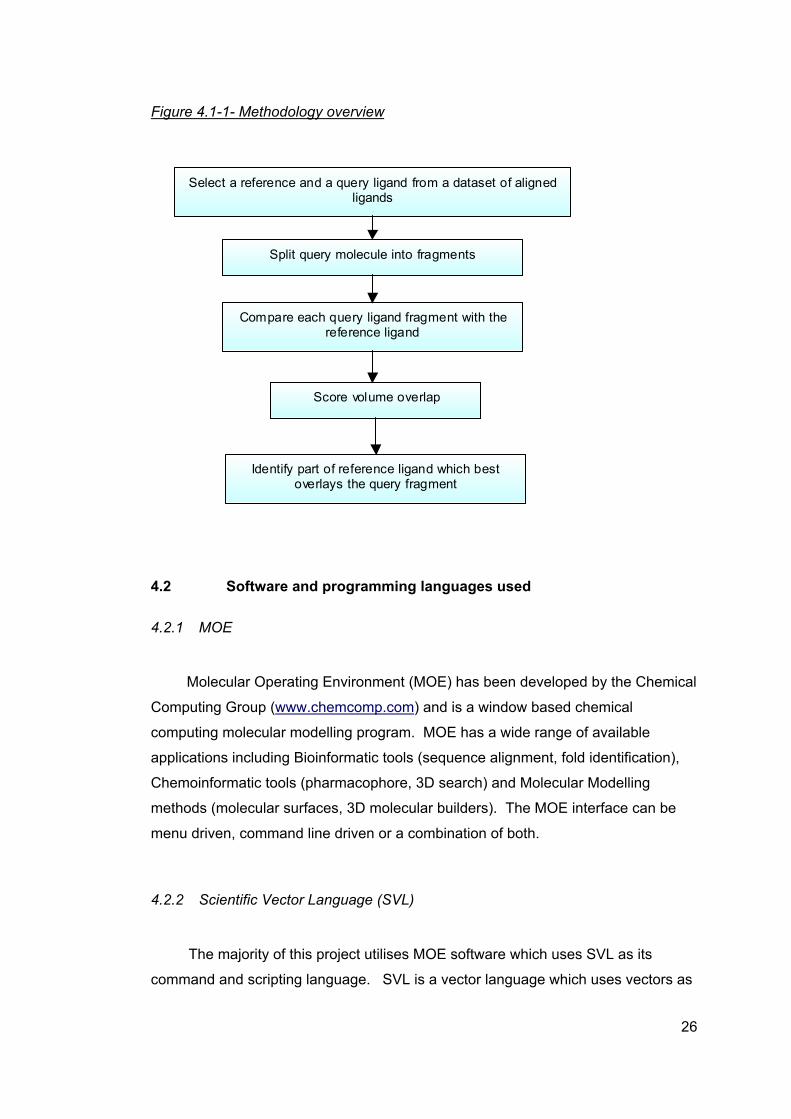
Figure 4.1-1- Methodology overview
Select a reference and a query ligand from a dataset of aligned ligands
Split query molecule into fragments
Compare each query ligand fragment with the reference ligand
Score volume overlap
Identify part of reference ligand which best overlays the query fragment
Score volume overlap
4.2 Software and programming languages used
4.2.1 MOE
Molecular Operating Environment (MOE) has been developed by the Chemical
Computing Group (www.chemcomp.com) and is a window based chemical
computing molecular modelling program. MOE has a wide range of available
applications including Bioinformatic tools (sequence alignment, fold identification),
Chemoinformatic tools (pharmacophore, 3D search) and Molecular Modelling
methods (molecular surfaces, 3D molecular builders). The MOE interface can be
menu driven, command line driven or a combination of both.
4.2.2 Scientific Vector Language (SVL)
The majority of this project utilises MOE software which uses SVL as its
command and scripting language. SVL is a vector language which uses vectors as
26
the primitive unit of operation. As opposed to other programming languages where
the primitive data unit is a scalar, vectors can be one of any number of possible data
structures built around scalar quantities (MOE Manual 2004). The SVL scripts
behind all the built-in MOE functions are available within the MOE documentation.
This means that users are able to modify and customize the scripts to fulfil their own
requirements.
The rationale behind using a vector language is that it is well suited to solving
problems involving intensive computations on large amounts of data. Using vectors
to manipulate data allows an operation to be carried out over an entire data set but
just using a single instruction (MOE Manual 2004).
4.3 Ligand Dataset
A protein database of X-ray crystallographic structures was clustered based on
protein sequence. All the proteins within one cluster were identical in sequence and
have a ligand bound. Although the proteins have identical sequences, they can
differ in conformation especially within their active site. Different ligands can cause
a protein to adopt different conformations. The binding modes of the ligands have
also been identified. In order to do this, it is important to understand the nature of
interactions between a protein and a ligand. These interactions were described in
chapter 3.2.
The proteins within a cluster were aligned by choosing a reference protein and
aligning all the other proteins to this protein. The ligands are then extracted from the
complexes resulting in a set of aligned ligands.
During the development of the functions described in the following sections, a
dataset of 35 ligands for the HIV1 reverse transcriptase inhibitor was used to test
the function. The aligned ligands had already been extracted and were therefore
ready to use. The results obtained from this dataset are described later.
The developed function was also run on internal Aventis databases but due to
confidentiality reasons the results cannot be shown within this report. The function
was also run on sets of ligands extracted from the PDB. As these structures are
publicly available the results are shown in a later chapter.
27
4.4 Splitting the ligands into fragments
In order to identify any potential bioisosteres, each of the extracted ligands
needs to be broken into fragments by breaking appropriate intramolecular bonds.
To manually split each ligand into fragments would be a time consuming
process, especially when large numbers of ligands are being analysed (as will be
the case here). Therefore, SVL scripts were written into order to automate and
ensure consistency of this process.
There are several ways of splitting a molecule into fragments, each having
different rules on which bonds should be broken during the splitting process. Each
method will lead to different numbers of fragments being created which could differ
structurally.
Whichever method is chosen, it is important to ensure that the fragments
created are meaningful and can be compared against other fragments or a
reference molecule in order to identify bioisosteres For example, splitting a
molecule down into its constituent atoms would not be constructive, as comparing
one atom against another would not yield meaningful bioisosteres. Once one
method was chosen, this was used throughout the rest of the project so ensuring
consistency when creating fragments and identifying bioisosteric pairs.
4.4.1 Splitting Molecule function
The first part of this project, therefore, involved determining how ligands
should be split into fragments i.e. identifying a set of rules for breaking the bonds
between atoms within the molecule. Once these rules had been established, a SVL
script was developed in order to automate the splitting process.
Two functions were developed in order to conduct this process. Developing
these functions was a good introduction to the SVL language and learning how to
construct scripts.
28
Only one of the functions is described here as this function was used in later
stages of the project. The function was developed based on learnings gained in
developing earlier versions of the function and analysing the results obtained.
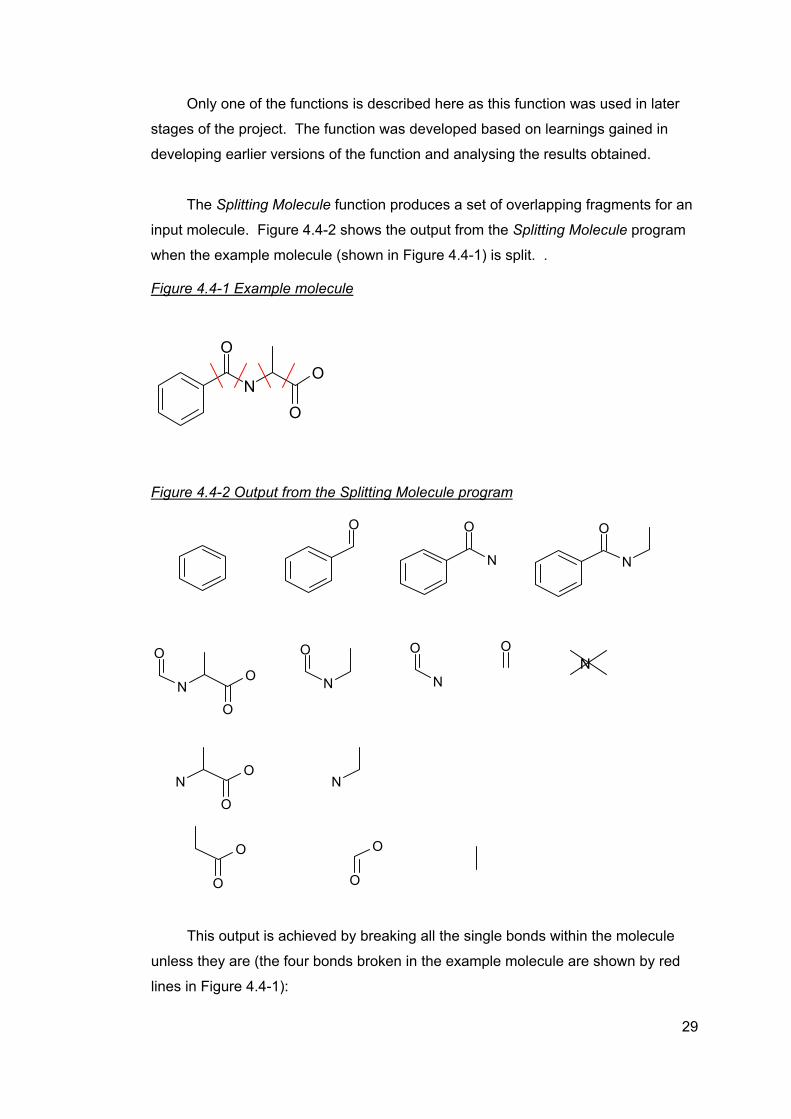
The Splitting Molecule function produces a set of overlapping fragments for an
input molecule. Figure 4.4-2 shows the output from the Splitting Molecule program
when the example molecule (shown in Figure 4.4-1) is split. .
Figure 4.4-1 Example molecule
N
O
O
O
Figure 4.4-2 Output from the Splitting Molecule program
O
N
O
O
O
O
N
O
N
N
O
N
O O
NO
ON
O
O
O
O
N
This output is achieved by breaking all the single bonds within the molecule
unless they are (the four bonds broken in the example molecule are shown by red
lines in Figure 4.4-1):
29
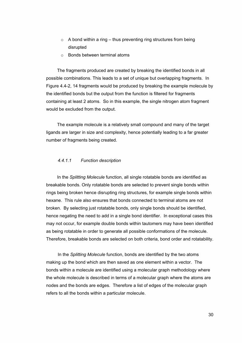
o A bond within a ring – thus preventing ring structures from being
disrupted
o Bonds between terminal atoms
The fragments produced are created by breaking the identified bonds in all
possible combinations. This leads to a set of unique but overlapping fragments. In
Figure 4.4-2, 14 fragments would be produced by breaking the example molecule by
the identified bonds but the output from the function is filtered for fragments
containing at least 2 atoms. So in this example, the single nitrogen atom fragment
would be excluded from the output.
The example molecule is a relatively small compound and many of the target
ligands are larger in size and complexity, hence potentially leading to a far greater
number of fragments being created.
4.4.1.1 Function description
In the Splitting Molecule function, all single rotatable bonds are identified as
breakable bonds. Only rotatable bonds are selected to prevent single bonds within
rings being broken hence disrupting ring structures, for example single bonds within
hexane. This rule also ensures that bonds connected to terminal atoms are not
broken. By selecting just rotatable bonds, only single bonds should be identified,
hence negating the need to add in a single bond identifier. In exceptional cases this
may not occur, for example double bonds within tautomers may have been identified
as being rotatable in order to generate all possible conformations of the molecule.
Therefore, breakable bonds are selected on both criteria, bond order and rotatability.
In the Splitting Molecule function, bonds are identified by the two atoms
making up the bond which are then saved as one element within a vector. The
bonds within a molecule are identified using a molecular graph methodology where
the whole molecule is described in terms of a molecular graph where the atoms are
nodes and the bonds are edges. Therefore a list of edges of the molecular graph
refers to all the bonds within a particular molecule.
30
Once all the bonds in the molecule have been identified and saved into ‘aBds’,
the single rotatable bonds are then filtered out and saved into variable ‘bond’. The
‘bond’ variable is a global variable in order to prevent it being reinitialised or
overwritten in recursive functions (Script 1 shows the relevant code).
Script 1: / local bds = tr xgraph atoms;
local bd = cat bds;
local aBds = split [get [atoms, bd], 2];
local ab =(app aRotatable aBds) and (app border aBds ==1);
bond = aBds | ab;/
As the function will need to process large amounts of data, it was important
for the code to be as efficient as possible. One of the hardest parts of the code was
attempting to prevent large numbers of duplicate fragments being generated. If the
all the identified bonds are broken in each recursion, this leads to the fragments
being duplicated a large number of times. It was therefore necessary to employ a
method of keeping track of which bonds have been broken in each iteration of the
main loop. Each time a bond has been broken in the main loop, the bond is flagged
and not broken again in any following recursive functions. Another global vector
‘bdLoop’ acts as a flag which tracks these broken bonds. ‘bdLoop’ is initialised as a
vector of zeros each corresponding to an identified breakable bond.
/bdLoop = rep [0, length bond];/
The identified bonds are then looped through and broken in turn. The
‘bdLoop’ variable is updated with a 1 replacing the 0 to reflect that this bond has
been cut and should not be cut again. A new global variable ‘toCutBonds’ is created
which stores only bonds which should be cut in the recursive function.
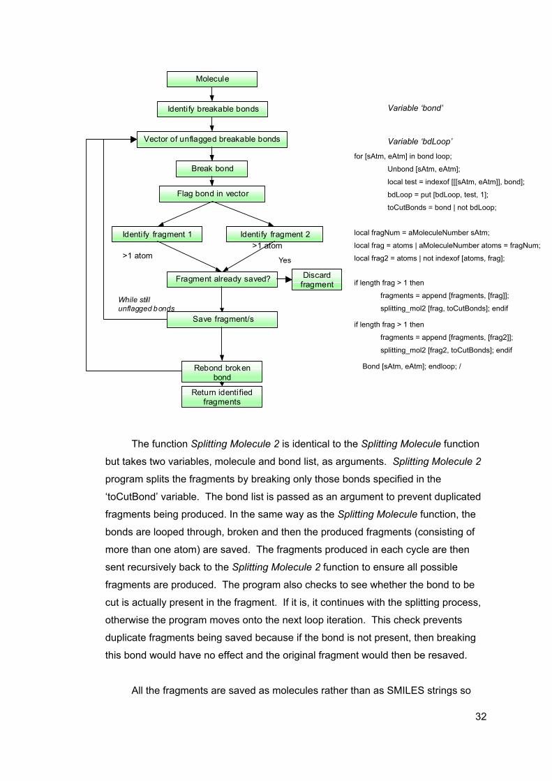
The two fragments (‘frag’, ‘frag2’) created from breaking a bond are saved into
the ‘fragments’ variable, provided they contain at least two atoms. Each fragment is
then passed as argument, along with ‘toCutBonds’, to the recursive function Splitting
Molecule 2 function (termed splitting_mol2 in the code). A flow diagram detailing
this process is shown below with the relevant code shown alongside.
31
Molecule
Identify breakable bonds
Vector of unflagged breakable bonds
Break bond
Flag bond in vector
Identify fragment 1 Identify fragment 2
Fragment already saved?
Save fragment/s
Discard fragment
Yes
Rebond broken bond
While still unflagged bonds
>1 atom >1 atom
Return identified fragments
for [sA
local fr
local fr
local fr
Bon
The function Splitting Molecule 2 is identical to the Spl
but takes two variables, molecule and bond list, as argumen
program splits the fragments by breaking only those bonds s
‘toCutBond’ variable. The bond list is passed as an argume
fragments being produced. In the same way as the Splitting
bonds are looped through, broken and then the produced fra
more than one atom) are saved. The fragments produced in
sent recursively back to the Splitting Molecule 2 function to e
fragments are produced. The program also checks to see w
cut is actually present in the fragment. If it is, it continues w
otherwise the program moves onto the next loop iteration. T
duplicate fragments being saved because if the bond is not
this bond would have no effect and the original fragment wo
All the fragments are saved as molecules rather than a
tm, eAtm] in bond loop;
Unbond [sAtm, eAtm];
local test = indexof [[[sAtm, eAtm]], bond];
bdLoop = put [bdLoop, test, 1];
toCutBonds = bond | not bdLoop;
Variable ‘bdLoop’
ag
ag
ag
d
itt
ts
p
nt
M
g
e
n
h
ith
h
pr
ul
s
Variable ‘bond’
Num = aMoleculeNumber sAtm;
= atoms | aMoleculeNumber atoms = fragNum;
2 = atoms | not indexof [atoms, frag];
if length frag > 1 then
fragments = append [fragments, [frag]];
splitting_mol2 [frag, toCutBonds]; endif
if length frag > 1 thenfragments = append [fragments, [frag2]];
splitting_mol2 [frag2, toCutBonds]; endif
[sAtm, eAtm]; endloop; /ing Molecule function
. Splitting Molecule 2
ecified in the
to prevent duplicated
olecule function, the
ments (consisting of
ach cycle are then
sure all possible
ether the bond to be
the splitting process,
is check prevents
esent, then breaking
d then be resaved.
SMILES strings so
32

preserving the 3D coordinates of the fragment. SMILES strings do not contain any
3D coordinate information about the fragment meaning that extracted fragments
could not then be overlaid onto a reference molecule as the coordinates, and hence
alignment information, has been lost. A filter is applied to the generated fragments,
namely one atom fragments are excluded from the output. A global variable
‘fragments’ is used to save all the fragments created during the program and is
returned by the function. All the generated fragments created from the Splitting
Molecule function are overlaid onto a reference molecule, without modifying the
original coordinates, and the overlap scored using the function described in the next
section.
4.5 Identifying fragment pairs
The next step in the process is to split a query molecule into fragments using
the Splitting Molecule function, and then compare each generated query fragment
with a reference molecule. For each comparison, the atoms within the reference
molecule which best overlay the query fragment are identified. As the fragment and
the reference molecule are already aligned then it is a case of scoring the best
overlap between the query fragment and sections of the reference molecule to
determine the best pairing of atoms.
In this project, the overlap will be calculated based on the degree to which the
two fragments overlap in terms of the volume of their constituent atoms. Fragments
with a high degree of overlap will occupy a similar position within the protein’s active
site and hence are assumed to have a similar role within the ligand. The fragments
do not necessarily have to be involved in intermolecular binding but can play other
important roles such as linker or scaffold roles. Therefore, we are only interested in
looking at the steric properties of the fragments when calculating similarity rather
than other properties such as hydrogen bonding properties.
In the Holiday et al. (2003) paper, described in Chapter 3.4, they found that the
atom descriptors, atomic weight and molar refractivity, discriminated between the
bioisosteric and nonbioisosteric groups best. As both these properties are related to
atom volume then the study can help to provide justification for basing the
identification of bioisosteres on volume.
33
4.5.1 Scoring overlap
There are many techniques available for calculating similarity between
molecules and are commonly used when aligning molecules and optimising the best
superimposition. These techniques use different methodologies for calculating
similarity and are based on different molecular properties such as steric,
electrostatic and hydrophobic field descriptors.
There are many studies which have looked at the problem of superimposing
ligands (both for rigid and flexible ligand alignment) and scoring the similarity
between them in order to optimise the superimposition. Only a brief overview is
given here of some of these techniques. Lemmen & Lengauer (2000) in their review
article provide a more in-depth review of these studies.
One of the earliest techniques is the Carbó method which uses structural
properties to calculate similarity using the Carbó index. Carbó originally used
quantum mechanically derived electron density as the measured property (Kotani &
Higashiura 2002) but the Carbó index can be applied to any molecular property that
can be calculated at any point around the molecule. The degree of similarity is
measured by aligning the two molecules so to maximise the overlap of the
corresponding properties (Bohl et al. 2002). There are some drawbacks with the
Carbó method, namely that electron density can be costly to compute and it was
discovered that it was not sufficiently discriminatory a property to use in similarity
searching (Leach & Gillet 2003).
Later techniques have involved using grid-based similarity calculations.
Molecules are surrounded by a rectilinear gird and the chosen property is calculated
at each vertices of the grid. This is an approximation as the property value is only
calculated at certain points rather than over the whole space. A drawback of these
methods is that in order to achieve reasonable computational speed the grids
employed tend to be coarse, hence affecting the accuracy of the calculation (Kotani
& Higashiura 2002).
Gaussian functions have been utilised to approximate the molecular
properties. Good & Richards (1993) describe a method where Gaussian functions
are first used to fit the curve of electron density against distance from atom nuclei.
34
These functions are then inserted into the Carbó index providing an analytical
evaluation of similarity. This leads to a significant reduction in the computational
time required to calculate the overlap between two aligned structures as the
similarity is measured analytically rather than numerically. Grant et al. (1996) also
describe a method for superimposition based on optimisation of van der Waals
overlap again using Gaussian functions.
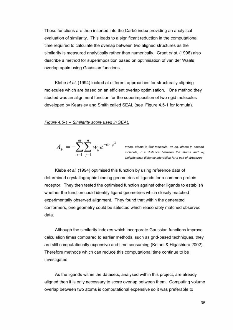
Klebe et al. (1994) looked at different approaches for structurally aligning
molecules which are based on an efficient overlap optimisation. One method they
studied was an alignment function for the superimposition of two rigid molecules
developed by Kearsley and Smith called SEAL (see Figure 4.5-1 for formula).
Figure 4.5-1 – Similarity score used in SEAL
∑∑=
−
=
−=m
i
rn
jijF
ijewA1 1
2α
Klebe et al. (1994) optimised this fu
determined crystallographic binding geom
receptor. They then tested the optimised
whether the function could identify ligand
experimentally observed alignment. They
conformers, one geometry could be selec
data.
Although the similarity indexes whic
calculation times compared to earlier met
are still computationally expensive and tim
Therefore methods which can reduce this
investigated.
As the ligands within the datasets, a
aligned then it is only necessary to score
overlap between two atoms is computatio
m=no. atoms in first molecule, n= no. atoms in second
molecule, r = distance between the atoms and wij
weights each distance interaction for a pair of structures
nction by using reference data of
etries of ligands for a common protein
function against other ligands to establish
geometries which closely matched
found that within the generated
ted which reasonably matched observed
h incorporate Gaussian functions improve
hods, such as grid-based techniques, they
e consuming (Kotani & Higashiura 2002).
computational time continue to be
nalysed within this project, are already
overlap between them. Computing volume
nal expensive so it was preferable to
35
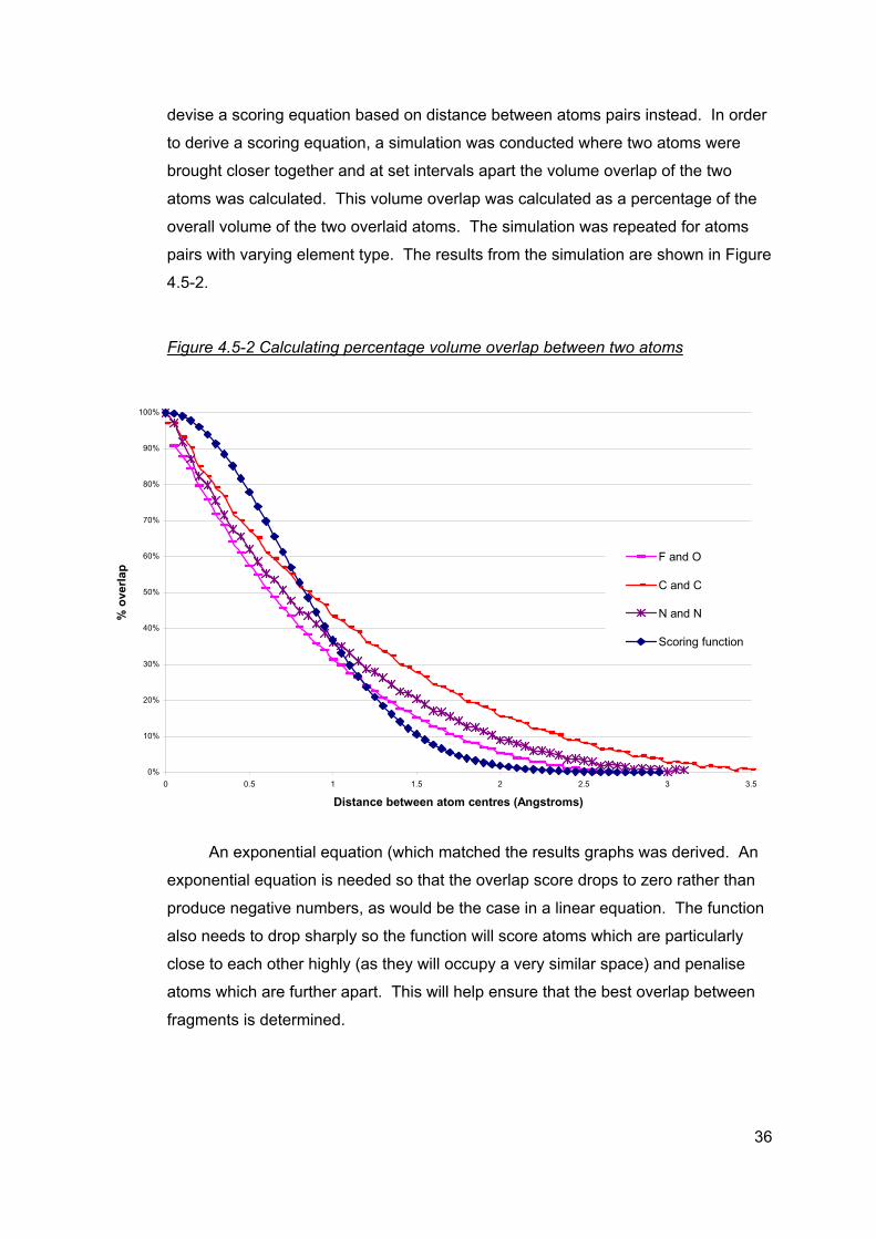
devise a scoring equation based on distance between atoms pairs instead. In order
to derive a scoring equation, a simulation was conducted where two atoms were
brought closer together and at set intervals apart the volume overlap of the two
atoms was calculated. This volume overlap was calculated as a percentage of the
overall volume of the two overlaid atoms. The simulation was repeated for atoms
pairs with varying element type. The results from the simulation are shown in Figure
4.5-2.
Figure 4.5-2 Calculating percentage volume overlap between two atoms
0%
10%
20%
30%
40%
50%
60%
70%
80%
90%
100%
0 0.5 1 1.5 2 2.5 3 3.5
Distance between atom centres (Angstroms)
% o
verla
p
F and O
C and C
N and N
Scoring function
An exponential equation (which matched the results graphs was derived. An
exponential equation is needed so that the overlap score drops to zero rather than
produce negative numbers, as would be the case in a linear equation. The function
also needs to drop sharply so the function will score atoms which are particularly
close to each other highly (as they will occupy a very similar space) and penalise
atoms which are further apart. This will help ensure that the best overlap between
fragments is determined.
36
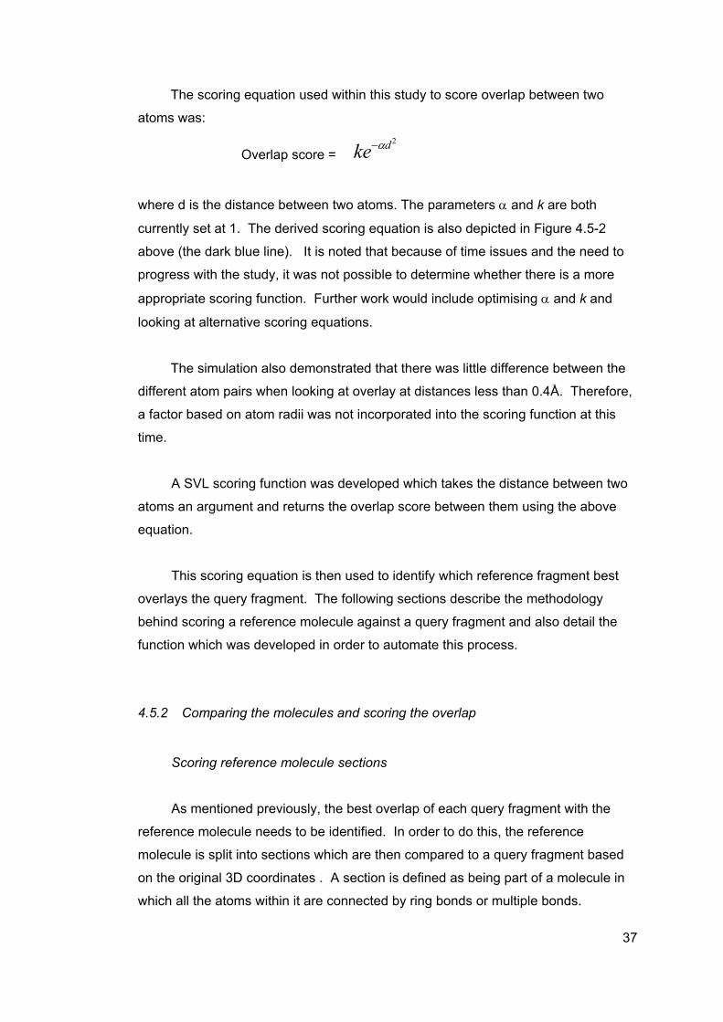
The scoring equation used within this study to score overlap between two
atoms was:
Overlap score = 2dke α−
where d is the distance between two atoms. The parameters α and k are both
currently set at 1. The derived scoring equation is also depicted in Figure 4.5-2
above (the dark blue line). It is noted that because of time issues and the need to
progress with the study, it was not possible to determine whether there is a more
appropriate scoring function. Further work would include optimising α and k and
looking at alternative scoring equations.
The simulation also demonstrated that there was little difference between the
different atom pairs when looking at overlay at distances less than 0.4Å. Therefore,
a factor based on atom radii was not incorporated into the scoring function at this
time.
A SVL scoring function was developed which takes the distance between two
atoms an argument and returns the overlap score between them using the above
equation.
This scoring equation is then used to identify which reference fragment best
overlays the query fragment. The following sections describe the methodology
behind scoring a reference molecule against a query fragment and also detail the
function which was developed in order to automate this process.
4.5.2 Comparing the molecules and scoring the overlap
Scoring reference molecule sections
As mentioned previously, the best overlap of each query fragment with the
reference molecule needs to be identified. In order to do this, the reference
molecule is split into sections which are then compared to a query fragment based
on the original 3D coordinates . A section is defined as being part of a molecule in
which all the atoms within it are connected by ring bonds or multiple bonds.
37
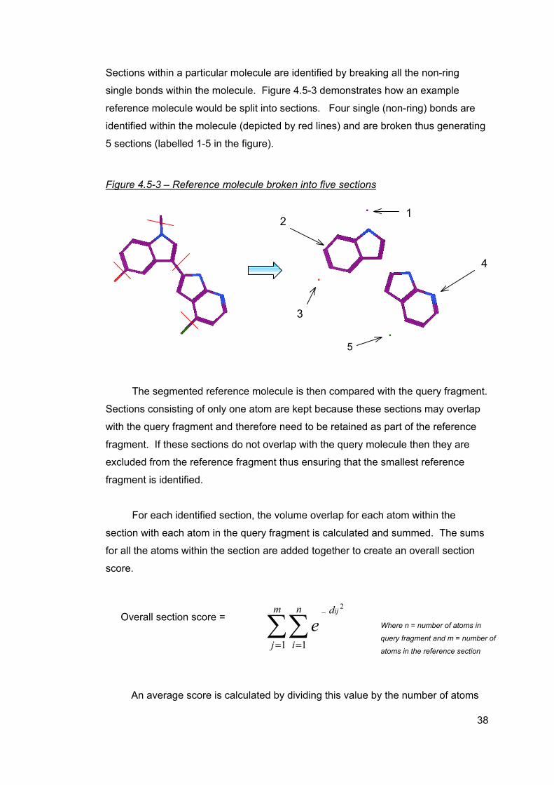
Sections within a particular molecule are identified by breaking all the non-ring
single bonds within the molecule. Figure 4.5-3 demonstrates how an example
reference molecule would be split into sections. Four single (non-ring) bonds are
identified within the molecule (depicted by red lines) and are broken thus generating
5 sections (labelled 1-5 in the figure).
Figure 4.5-3 – Reference molecule broken into five sections
1
5
3
2
4
The segmented reference molecule is then compared with the query fragment.
Sections consisting of only one atom are kept because these sections may overlap
with the query fragment and therefore need to be retained as part of the reference
fragment. If these sections do not overlap with the query molecule then they are
excluded from the reference fragment thus ensuring that the smallest reference
fragment is identified.
For each identified section, the volume overlap for each atom within the
section with each atom in the query fragment is calculated and summed. The sums
for all the atoms within the section are added together to create an overall section
score.
∑∑= =
−m
j
n
i
dije
1 1
2Overall section score =
An average score is calculated by dividing this value b
Where n = number of atoms in
query fragment and m = number of
atoms in the reference section
y the number of atoms
38
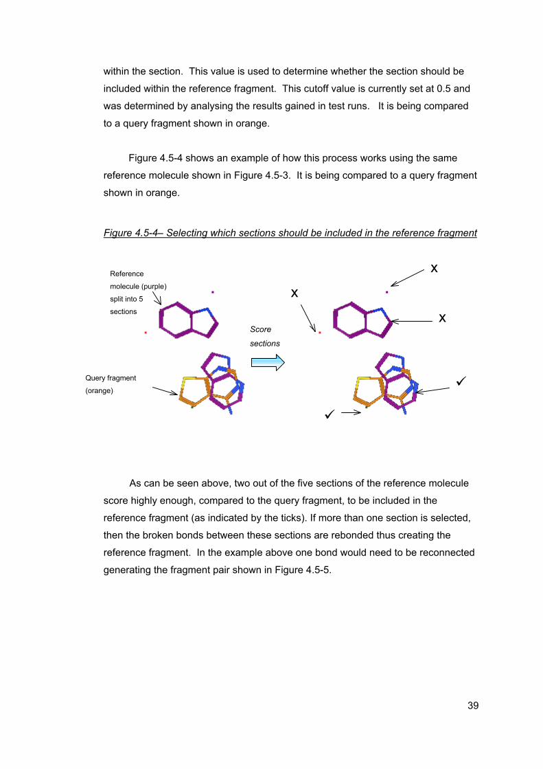
within the section. This value is used to determine whether the section should be
included within the reference fragment. This cutoff value is currently set at 0.5 and
was determined by analysing the results gained in test runs. It is being compared
to a query fragment shown in orange.
Figure 4.5-4 shows an example of how this process works using the same
reference molecule shown in Figure 4.5-3. It is being compared to a query fragment
shown in orange.
Figure 4.5-4– Selecting which sections should be included in the reference fragment
x
Query
(orang
x
s
r
t
r
g
Reference
molecule (purple)
split into 5
sections
x
fragment
e)
Score
sections
As can be seen above, two out of the five sections of the reference molecule
core highly enough, compared to the query fragment, to be included in the
eference fragment (as indicated by the ticks). If more than one section is selected,
hen the broken bonds between these sections are rebonded thus creating the
eference fragment. In the example above one bond would need to be reconnected
enerating the fragment pair shown in Figure 4.5-5.
39
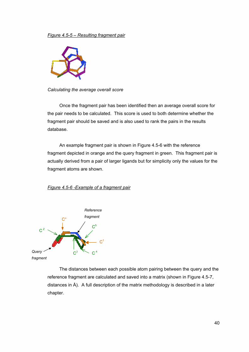
Figure 4.5-5 – Resulting fragment pair
Calculating the average overall score
Once the fragment pair has been identified then an average overall score for
the pair needs to be calculated. This score is used to both determine whether the
fragment pair should be saved and is also used to rank the pairs in the results
database.
An example fragment pair is shown in Figure 4.5-6 with the reference
fragment depicted in orange and the query fragment in green. This fragment pair is
actually derived from a pair of larger ligands but for simplicity only the values for the
fragment atoms are shown.
Figure 4.5-6 -Example of a fragment pair
C 2
Query
fragment
C°
C3 C 4
C5
Reference
fragment
C1
The distances between each possible atom pairing between the query and the
reference fragment are calculated and saved into a matrix (shown in Figure 4.5-7,
distances in Å). A full description of the matrix methodology is described in a later
chapter.
40
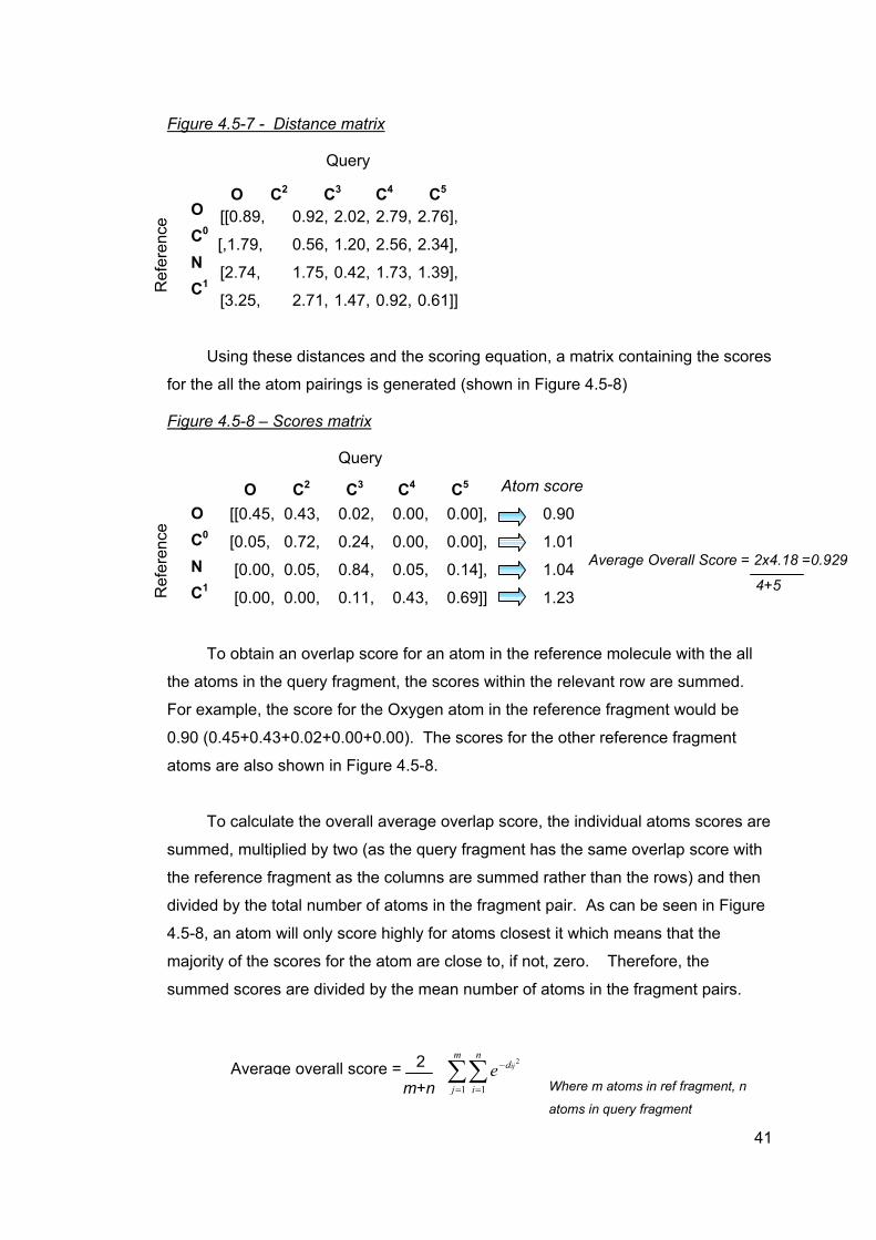
Figure 4.5-7 - Distance matrix
Query
[
[
O C0
N C1 R
efer
ence
[
[
Us
for the a
Figure 4
O C0
N C1 R
efer
ence
To
the atom
For exa
0.90 (0.
atoms a
To
summed
the refe
divided
4.5-8, a
majority
summed
O C2 C3 C4 C5
[0.89, 0.92, 2.02, 2.79, 2.76],,1.79, 0.56, 1.20, 2.56, 2.34],
2.74, 1.75, 0.42, 1.73, 1.39],
3.25, 2.71, 1.47, 0.92, 0.61]]
ing these distances and the scoring equation, a matrix containing the scores
ll the atom pairings is generated (shown in Figure 4.5-8)
.5-8 – Scores matrix
Query
Atom score [
[
o
s
m
45
re
c
,
re
by
n
o
s
O C2 C3 C4 C5
[0.45, 0.43, 0.02, 0.00, 0.00], 0.900.05, 0.72, 0.24, 0.00, 0.00], 1.01
[0.00, 0.05, 0.84, 0.05, 0.14], 1.04
[0.00, 0.00, 0.11, 0.43, 0.69]] 1.23
Average Overall Score = 2x4.18 =0.929
4+5
btain an overlap score for an atom in the reference molecule with the all
in the query fragment, the scores within the relevant row are summed.
ple, the score for the Oxygen atom in the reference fragment would be
+0.43+0.02+0.00+0.00). The scores for the other reference fragment
also shown in Figure 4.5-8.
alculate the overall average overlap score, the individual atoms scores are
multiplied by two (as the query fragment has the same overlap score with
nce fragment as the columns are summed rather than the rows) and then
the total number of atoms in the fragment pair. As can be seen in Figure
atom will only score highly for atoms closest it which means that the
f the scores for the atom are close to, if not, zero. Therefore, the
cores are divided by the mean number of atoms in the fragment pairs.
∑∑= =
−m
j
n
i
dije1 1
2=
m+nAverage overall score
Where m atoms in ref fragment, natoms in query fragment
2
41
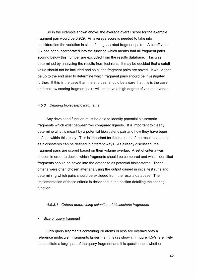
So in the example shown above, the average overall score for the example
fragment pair would be 0.929. An average score is needed to take into
consideration the variation in size of the generated fragment pairs. A cutoff value
0.7 has been incorporated into the function which means that all fragment pairs
scoring below this number are excluded from the results database. This was
determined by analysing the results from test runs. It may be decided that a cutoff
value should not be included and so all the fragment pairs are saved. It would then
be up to the end user to determine which fragment pairs should be investigated
further. It this is the case than the end user should be aware that this is the case
and that low scoring fragment pairs will not have a high degree of volume overlap.
4.5.3 Defining bioisosteric fragments
Any developed function must be able to identify potential bioisosteric
fragments which exist between two compared ligands. It is important to clearly
determine what is meant by a potential bioisosteric pair and how they have been
defined within this study. This is important for future users of the results database
as bioisosteres can be defined in different ways. As already discussed, the
fragment pairs are scored based on their volume overlap. A set of criteria was
chosen in order to decide which fragments should be compared and which identified
fragments should be saved into the database as potential bioisosteres. These
criteria were often chosen after analysing the output gained in initial test runs and
determining which pairs should be excluded from the results database. The
implementation of these criteria is described in the section detailing the scoring
function.
4.5.3.1 Criteria determining selection of bioisosteric fragments
• Size of query fragment
Only query fragments containing 20 atoms or less are overlaid onto a
reference molecule. Fragments larger than this (as shown in Figure 4.5-9) are likely
to constitute a large part of the query fragment and it is questionable whether
42
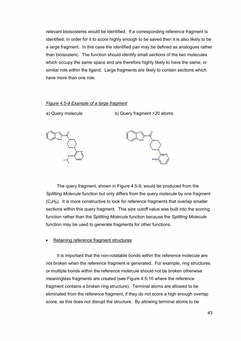
relevant bioisosteres would be identified. If a corresponding reference fragment is
identified, in order for it to score highly enough to be saved then it is also likely to be
a large fragment. In this case the identified pair may be defined as analogues rather
than bioisosteric. The function should identify small sections of the two molecules
which occupy the same space and are therefore highly likely to have the same, or
similar role within the ligand. Large fragments are likely to contain sections which
have more than one role.
Figure 4.5-9 Example of a large fragment
a) Query molecule b) Query fragment >20 atoms
The query fragment, shown in Figure 4.5-9, would be produced from the
Splitting Molecule function but only differs from the query molecule by one fragment
(C3H8). It is more constructive to look for reference fragments that overlap smaller
sections within this query fragment. This size cutoff value was built into the scoring
function rather than the Splitting Molecule function because the Splitting Molecule
function may be used to generate fragments for other functions.
• Retaining reference fragment structures
It is important that the non-rotatable bonds within the reference molecule are
not broken when the reference fragment is generated. For example, ring structures
or multiple bonds within the reference molecule should not be broken otherwise
meaningless fragments are created (see Figure 4.5-10 where the reference
fragment contains a broken ring structure). Terminal atoms are allowed to be
eliminated from the reference fragment, if they do not score a high enough overlap
score, as this does not disrupt the structure. By allowing terminal atoms to be
43
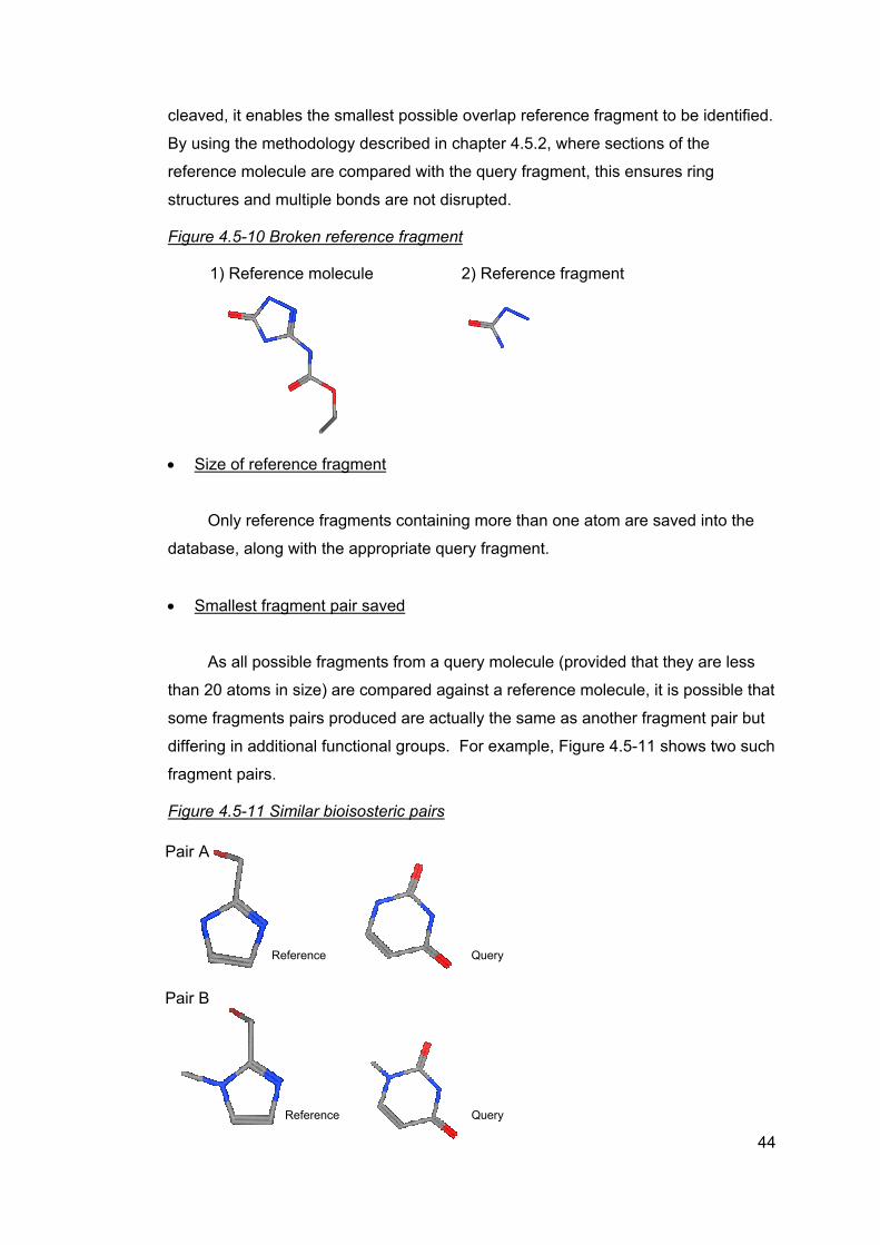
cleaved, it enables the smallest possible overlap reference fragment to be identified.
By using the methodology described in chapter 4.5.2, where sections of the
reference molecule are compared with the query fragment, this ensures ring
structures and multiple bonds are not disrupted.
Figure 4.5-10 Broken reference fragment
1) Reference molecule 2) Reference fragment
• Size of reference fragment
Only reference fragments containing more than one atom are saved into the
database, along with the appropriate query fragment.
• Smallest fragment pair saved
As all possible fragments from a query molecule (provided that they are less
than 20 atoms in size) are compared against a reference molecule, it is possible that
some fragments pairs produced are actually the same as another fragment pair but
differing in additional functional groups. For example, Figure 4.5-11 shows two such
fragment pairs.
Figure 4.5-11 Similar bioisosteric pairs
A
PairB
PairReference
Query
Query Reference44
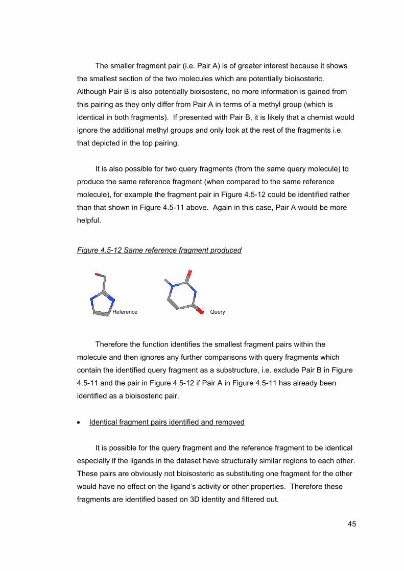
The smaller fragment pair (i.e. Pair A) is of greater interest because it shows
the smallest section of the two molecules which are potentially bioisosteric.
Although Pair B is also potentially bioisosteric, no more information is gained from
this pairing as they only differ from Pair A in terms of a methyl group (which is
identical in both fragments). If presented with Pair B, it is likely that a chemist would
ignore the additional methyl groups and only look at the rest of the fragments i.e.
that depicted in the top pairing.
It is also possible for two query fragments (from the same query molecule) to
produce the same reference fragment (when compared to the same reference
molecule), for example the fragment pair in Figure 4.5-12 could be identified rather
than that shown in Figure 4.5-11 above. Again in this case, Pair A would be more
helpful.
Figure 4.5-12 Same reference fragment produced
The
molecule
contain th
4.5-11 an
identified
• Identic
It is
especially
These pa
would hav
fragments
Reference
refore the function identifies th
and then ignores any further c
e identified query fragment as
d the pair in Figure 4.5-12 if P
as a bioisosteric pair.
al fragment pairs identified an
possible for the query fragme
if the ligands in the dataset h
irs are obviously not bioisoste
e no effect on the ligand’s act
are identified based on 3D id
Query
e smallest fragment pairs within the
omparisons with query fragments which
a substructure, i.e. exclude Pair B in Figure
air A in Figure 4.5-11 has already been
d removed
nt and the reference fragment to be identical
ave structurally similar regions to each other.
ric as substituting one fragment for the other
ivity or other properties. Therefore these
entity and filtered out.
45
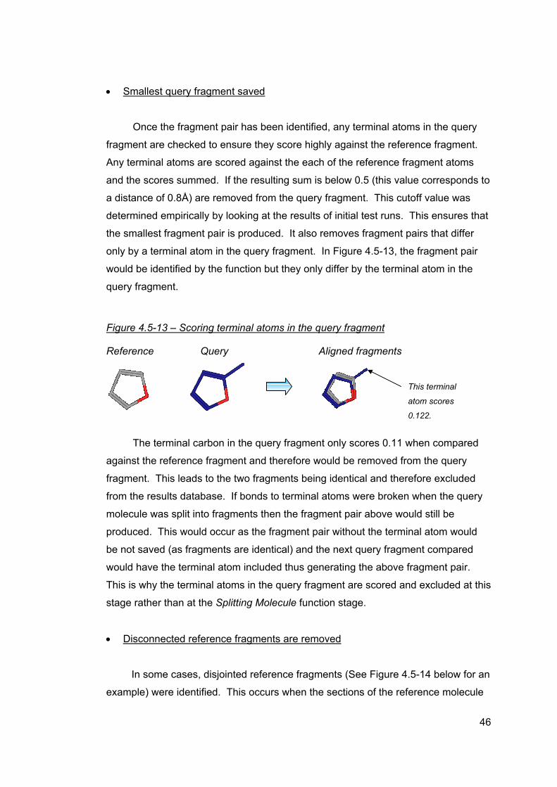
• Smallest query fragment saved
Once the fragment pair has been identified, any terminal atoms in the query
fragment are checked to ensure they score highly against the reference fragment.
Any terminal atoms are scored against the each of the reference fragment atoms
and the scores summed. If the resulting sum is below 0.5 (this value corresponds to
a distance of 0.8Å) are removed from the query fragment. This cutoff value was
determined empirically by looking at the results of initial test runs. This ensures that
the smallest fragment pair is produced. It also removes fragment pairs that differ
only by a terminal atom in the query fragment. In Figure 4.5-13, the fragment pair
would be identified by the function but they only differ by the terminal atom in the
query fragment.
Figure 4.5-13 – Scoring terminal atoms in the query fragment
Reference Query Aligned fragments
This terminal
atom scores
0.122.
The terminal carbon in the query fragment only scores 0.11 when compared
against the reference fragment and therefore would be removed from the query
fragment. This leads to the two fragments being identical and therefore excluded
from the results database. If bonds to terminal atoms were broken when the query
molecule was split into fragments then the fragment pair above would still be
produced. This would occur as the fragment pair without the terminal atom would
be not saved (as fragments are identical) and the next query fragment compared
would have the terminal atom included thus generating the above fragment pair.
This is why the terminal atoms in the query fragment are scored and excluded at this
stage rather than at the Splitting Molecule function stage.
• Disconnected reference fragments are removed
In some cases, disjointed reference fragments (See Figure 4.5-14 below for an
example) were identified. This occurs when the sections of the reference molecule
46
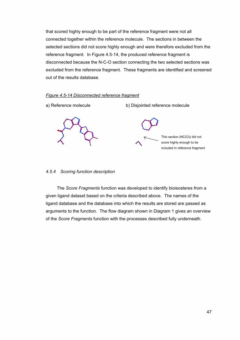
that scored highly enough to be part of the reference fragment were not all
connected together within the reference molecule. The sections in between the
selected sections did not score highly enough and were therefore excluded from the
reference fragment. In Figure 4.5-14, the produced reference fragment is
disconnected because the N-C-O section connecting the two selected sections was
excluded from the reference fragment. These fragments are identified and screened
out of the results database.
Figure 4.5-14 Disconnected reference fragment
a) Reference molecule b) Disjointed reference molecule
This section (NC(O)) did not
score highly enough to be
included in reference fragment
4.5.4 Scoring function description
The Score Fragments function was developed to identify bioisosteres from a
given ligand dataset based on the criteria described above. The names of the
ligand database and the database into which the results are stored are passed as
arguments to the function. The flow diagram shown in Diagram 1 gives an overview
of the Score Fragments function with the processes described fully underneath.
47

Diagram 1 Generating fragment pairs
S et Reference m olecule
Ligan d DataS et
S et as Query m olecule
Ide ntify bre akable bon ds Determ ine sec tions (as exp la ined in 4 .5 .2 )
Que ry
S plit query m olecule into fragm ents
Com pa re qu ery fragm ent with re fe rence m olecule
S core o verla p for e ach re fe rence sec tion
Calculate dis tance m atrix fo r re fe rence a nd qu ery m olecule
Calculate scorin g func tion m at rix fo r re fe re nce and q ue ry m olecule
Re fe rence frag m ent identifi ed
Calculate o ve rall o verla p score fo r re fe re nce frag m ent
Do the fra gm e nt pair m eet set c riteria
S a ve fra gm ent pair into databas e
Re fe rence
Fragment <2 atoms
Discard reference fragm ent
Fragment =>2 atoms
Score > 0.7
No
Y es
Wh ils t s til l que ry fragm ents loop
M o ve o n to nex t query m olecul e
Wh ils t s til l ligands in query da tas e t loop
M o ve o n to nex t re ference m olecule
Wh ils t s till ligands in re fe rence da tas e t loop
Sc ore =< 0.7
Y es
48
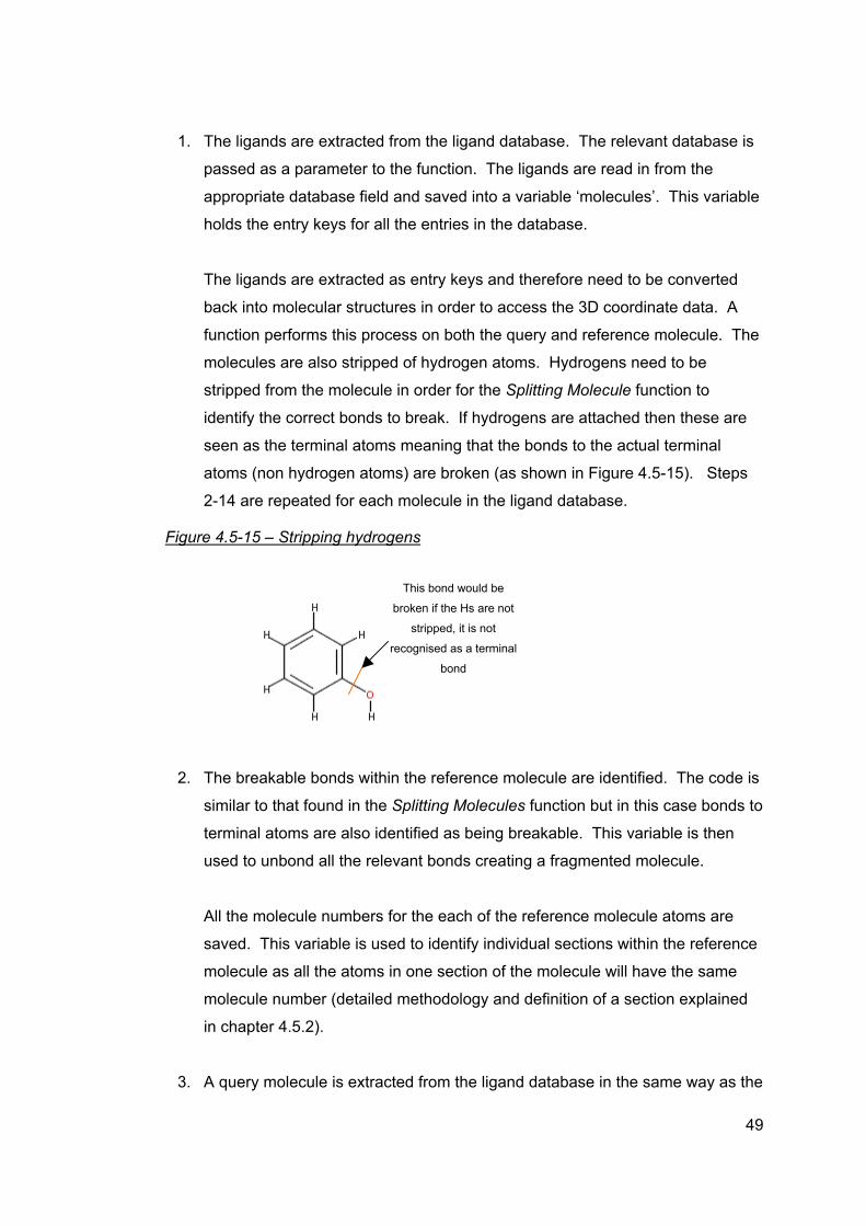
1. The ligands are extracted from the ligand database. The relevant database is
passed as a parameter to the function. The ligands are read in from the
appropriate database field and saved into a variable ‘molecules’. This variable
holds the entry keys for all the entries in the database.
The ligands are extracted as entry keys and therefore need to be converted
back into molecular structures in order to access the 3D coordinate data. A
function performs this process on both the query and reference molecule. The
molecules are also stripped of hydrogen atoms. Hydrogens need to be
stripped from the molecule in order for the Splitting Molecule function to
identify the correct bonds to break. If hydrogens are attached then these are
seen as the terminal atoms meaning that the bonds to the actual terminal
atoms (non hydrogen atoms) are broken (as shown in Figure 4.5-15). Steps
2-14 are repeated for each molecule in the ligand database.
Figure 4.5-15 – Stripping hydrogens
b
r
2. The breakable bonds within
similar to that found in the S
terminal atoms are also ide
used to unbond all the relev
All the molecule numbers fo
saved. This variable is use
molecule as all the atoms in
molecule number (detailed
in chapter 4.5.2).
3. A query molecule is extract
This bond would be
roken if the Hs are not
stripped, it is not
ecognised as a terminal
bond
the reference molecule are identified. The code is
plitting Molecules function but in this case bonds to
ntified as being breakable. This variable is then
ant bonds creating a fragmented molecule.
r the each of the reference molecule atoms are
d to identify individual sections within the reference
one section of the molecule will have the same
methodology and definition of a section explained
ed from the ligand database in the same way as the
49
reference molecules are. The reference and the query molecules come from
the same database. Again hydrogen atoms are stripped from the molecule.
Steps 5-14 are repeated for each molecule in the ligand database.
Comparisons between identical ligands are excluded at this stage.
4. A distance matrix is computed for the selected reference and query molecule
and contains distances between each atom in the reference molecule and
each atom in the query molecule (see following section for a detailed
explanation of the methodology).
5. An overlap score matrix is computed for the selected reference and query
molecule using the distance matrix generated in Step 4 and the scoring
equation (explained in 4.5.1).
6. Matrices comparing atoms within the reference and query molecules are
created. Each atom in the reference molecule is compared to the closest atom
in the query molecule. One matrix shows whether the paired atoms have the
same element type and the other shows whether the paired atoms have the
same geometry (e.g. sp2,sp3). These matrices are used later to determine
whether the reference and the query fragments are identical.
7. The query molecule is then split into fragments using the previously defined
Splitting Molecule function. The ‘fragment’ variable is sorted in increasing size
order to ensure that the smallest fragments are overlaid first. Each fragment is
tested to make sure it does not contain an already saved query fragment as a
substructure. This ensures that the criteria regarding the smallest fragment
pair being generated is met. Fragments containing more than 20 atoms are
filtered out at this stage. The relevant query fragments are then looped
through and aligned with the reference molecule.
8. A matrix containing the scores for just the query fragment atoms compared to
the reference fragment is generated. This means that only the scores
corresponding to the query fragment are extracted from the overall score
matrix. This then means that just the query fragment can be compared to the
reference ligand.
50
9. For each reference molecule section, the overlap of each atom with all the
atoms in the query fragment is calculated. The methodology behind this is
explained in chapter 4.5.2. Only sections with an averaged score of more
than a specified value (0.5) are included in the reference fragment. For
selected sections, the appropriate molecule number is saved and these will be
used to generate the appropriate reference fragment (in step 10). The
molecule numbers corresponding to the selected sections are identified along
with the sum of all the scores for all the atoms in the selected sections.
10. The fragment within the reference molecule which matches the query molecule
is then identified. The relevant sections of the reference molecule are selected
using the molecule numbers saved in Step 11.
11. Once the complete reference fragment has been identified, then an average
score is calculated. See chapter 4.5.2 for an explanation behind this
methodology.
12. A cutoff value is included to filter out only the highest scoring fragment pairs.
Only fragment pairs with an overall average score (as calculated in Step 11) of
over 0.7 are saved into the results database. This cutoff value was chosen
based on results obtained in test runs. Also reference fragments containing
less than 2 atoms are filtered out.
13. Fragment pairs which contain identical fragments, in terms of atom type and
geometry, are filtered out using the matrices generated in Step 6.
14. The fragment pairs which satisfy all the criteria (as specified in chapter 4.5.3.1)
are then saved into a database (described below) along with the original
reference and query molecules and their average overlap score.
4.5.5 Development and modifications of the function
The Scoring Fragments function underwent many modifications to increase its
efficiency and correct errors discovered during its development.
51

4.5.5.1 Retaining reference fragment structure
As mentioned in the criteria section, it was important to ensure that structures
within the reference fragment were not disrupted, e.g. ring structures or double
bonds. Originally the overlap score was calculated for each atom in the reference
molecule against each atom in the query fragment (within 2.5Å) and all the scores
were summed together for each reference molecule atom. Reference atoms with a
sum score over 0.5 were then identified as being part of the reference fragment.
This was repeated for each reference molecule atom. In order not to produce
disconnected fragment (one of the criteria described above), it then meant that once
these atoms were identified it necessary to ascertain all the other atoms in same
section of the reference molecule.
As whole sections had to be included in the reference fragment, the
methodology was changed so that the overlap score was calculated for each
reference molecule section instead (as explained in chapter 4.5.2). This simplified
the function and ensures that the ring structures or multiple bonds within the
reference molecule are not disrupted.
4.5.5.2 Matrix methodology
The overlap between each atom in the reference molecule and each query
fragment atom can be calculated each time a new query fragment is compared.
However, this methodology would be inefficient, as the same overlap score would
be repeatedly calculated because the same atoms will keep appearing in the query
fragments. If a different overlap scoring equation is utilised which is more time
consuming than the current scoring equation, then this will slow the program down
unnecessarily. Therefore, a more efficient method is to calculate the overlap scores
once for all possible pairings of atoms between the reference and query molecule.
Once these have been calculated, the scores can be accessed within each query
fragment loop.
In order to implement this methodology, matrices were utilised within the
52

function. Matrices in SVL are represented by a nested vector. .
Matrix = becomes a vector of rows m = [[a,b,c,d], [e,f,g,h],[i,j,k,l]]
ijklefghabcd
Therefore an r x c matrix has r (number of rows) elements each of which is
length c (number of columns). Row (i) can be extracted using the notation m(i) and
column j can be extracted similarly from the transformed matrix.
In the Score Fragments function, matrices are used to show all the possible
pairings of reference and query molecule atoms. For example, if the reference
molecule has 4 atoms (a,b,c,d) and the query molecule has 4 atoms (e,f,g,h) then all
the possible pairing are shown in the matrix below (Figure 4.5-16).
Figure 4.5-16 Comparison matrix
e f g h a
b
c
d
ae af ag ah
be bf ag ah
ce cf cg ch
de df dg dh
Query atoms
Ref atoms
This matrix structure can then be used to represent pairings of different
features or properties between the atoms of the two molecules. Several matrices
are created during the scoring function.
- Distance matrix - contains all the distances between each of the atoms in two
molecules. This matrix is only generated once for each reference and query
molecule pairing.
- Scores matrix – the distance matrix is then used to create an overlap score
matrix (as in Figure 4.5-17 below) that contains all the overlap scores for all the
atom pairs. Originally, the scores for atom pairs less than 2.5Å apart were
calculated which involved filtering out these distances from the distance matrix.
It is not necessary to do this as the score value for atoms over 2.5 Å is actually
53
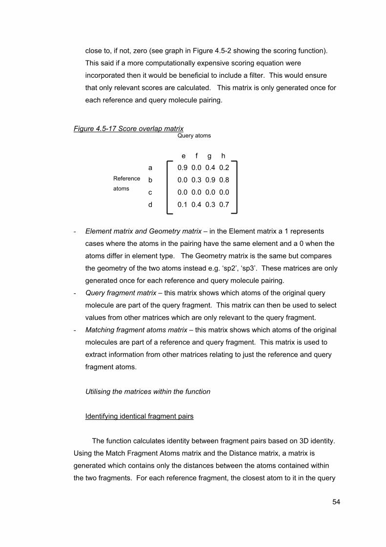
close to, if not, zero (see graph in Figure 4.5-2 showing the scoring function).
This said if a more computationally expensive scoring equation were
incorporated then it would be beneficial to include a filter. This would ensure
that only relevant scores are calculated. This matrix is only generated once for
each reference and query molecule pairing.
Figure 4.5-17 Score overlap matrix Query atoms
e f g h
- Elemen
cases w
atoms d
the geo
generat
- Query fr
molecul
values f
- Matchin
molecul
extract i
fragmen
Utilising
Identifyi
The fu
Using the M
generated w
the two frag
Reference
atoms
d
t matrix and Geomet
here the atoms in th
iffer in element type.
metry of the two atom
ed once for each refe
agment matrix – this
e are part of the que
rom other matrices w
g fragment atoms m
es are part of a refer
nformation from othe
t atoms.
the matrices within
ng identical fragmen
nction calculates ide
atch Fragment Atom
hich contains only t
ments. For each ref
0.9 0.0 0.4 0.2
0.0 0.3 0.9 0.8
0.0 0.0 0.0 0.0
0.1 0.4 0.3 0.7
a
b
c
ry matrix – in the Element matrix a 1 represents
e pairing have the same element and a 0 when the
The Geometry matrix is the same but compares
s instead e.g. ‘sp2’, ‘sp3’. These matrices are only
rence and query molecule pairing.
matrix shows which atoms of the original query
ry fragment. This matrix can then be used to select
hich are only relevant to the query fragment.
atrix – this matrix shows which atoms of the original
ence and query fragment. This matrix is used to
r matrices relating to just the reference and query
the function
t pairs
ntity between fragment pairs based on 3D identity.
s matrix and the Distance matrix, a matrix is
he distances between the atoms contained within
erence fragment, the closest atom to it in the query
54
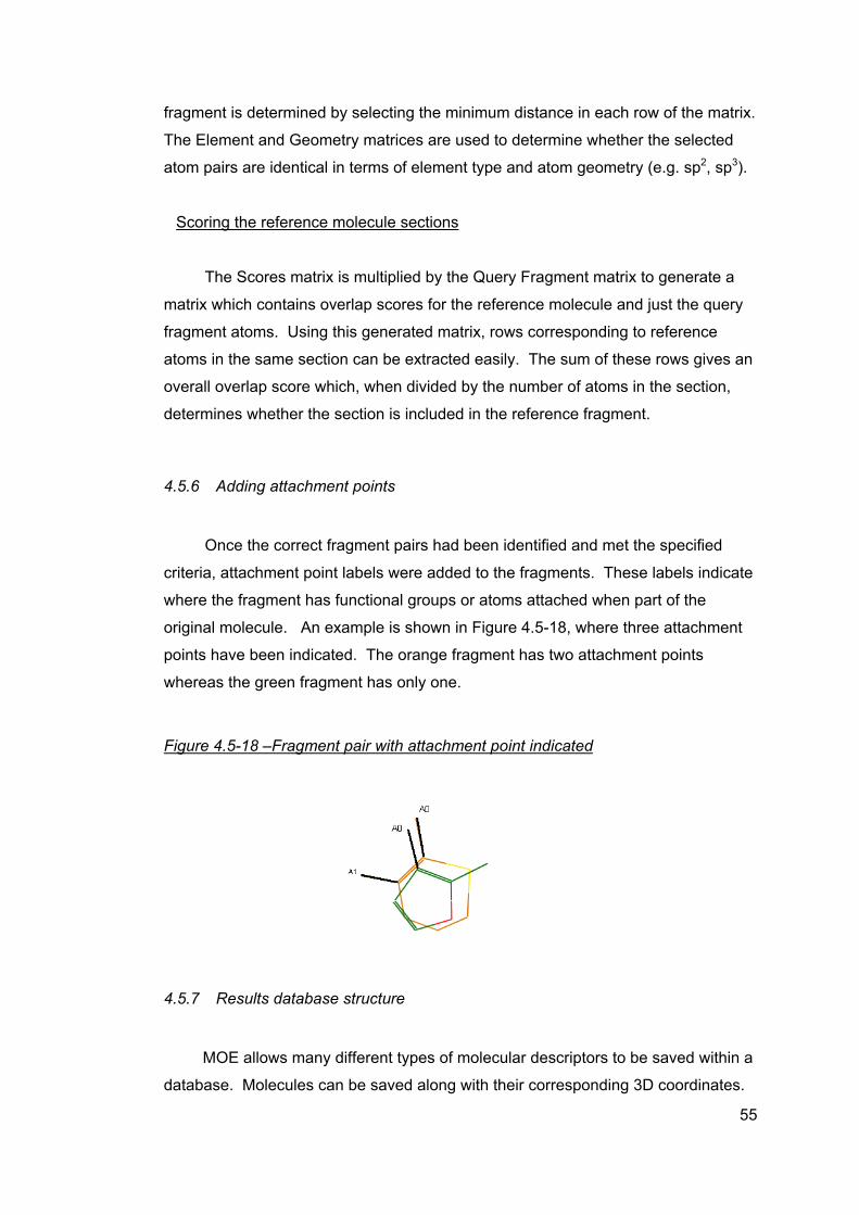
fragment is determined by selecting the minimum distance in each row of the matrix.
The Element and Geometry matrices are used to determine whether the selected
atom pairs are identical in terms of element type and atom geometry (e.g. sp2, sp3).
Scoring the reference molecule sections
The Scores matrix is multiplied by the Query Fragment matrix to generate a
matrix which contains overlap scores for the reference molecule and just the query
fragment atoms. Using this generated matrix, rows corresponding to reference
atoms in the same section can be extracted easily. The sum of these rows gives an
overall overlap score which, when divided by the number of atoms in the section,
determines whether the section is included in the reference fragment.
4.5.6 Adding attachment points
Once the correct fragment pairs had been identified and met the specified
criteria, attachment point labels were added to the fragments. These labels indicate
where the fragment has functional groups or atoms attached when part of the
original molecule. An example is shown in Figure 4.5-18, where three attachment
points have been indicated. The orange fragment has two attachment points
whereas the green fragment has only one.
Figure 4.5-18 –Fragment pair with attachment point indicated
4.5.7 Results database structure
MOE allows many different types of molecular descriptors to be saved within a
database. Molecules can be saved along with their corresponding 3D coordinates.
55
This is important for this study as conserving the 3D coordinates of the ligand
fragments is important in order to preserve the alignment data. A similar ligand
could have different conformations depending on which protein it is bound to. Only
fragment pairs which satisfy the criteria described previously are saved into the
database. One results database is created per target protein. The results database
has seven fields:
• Pair_id – a unique number which can identify each pair of fragments
• Reference_molecule – molecule which acted as reference onto which
the query fragments were overlaid.
• Query_molecule – the complete molecule with which the query
fragment originated from.
• Query_frag – query fragment which was overlaid on the reference
molecule
• Ref_frag – corresponding fragment within the reference molecule
which the Query_frag matched to
• Score – average overlap score associated with the fragment pair
• Aligned_Frags – the reference and query fragment are aligned and
displayed
If the ligands within the test dataset are structurally similar to one another then
it is likely that the same fragment pairs will be identified in different ligands. All the
fragment pairs are saved meaning so that it is possible to trace all the ligands which
contain a particular fragment pair.
4.5.8 Limitations with the scoring function
4.5.8.1 Repetition
There is repetition in the creation of the overlap score matrices, for example
when molecule A is compared to molecule B, a score matrix is produced but this is
the same matrix created when molecule B is compared to molecule A. Therefore
the same matrix has been created twice. At present a method for preventing this
duplication of matrices has not been devised but it is not necessary to do currently
as the function is executing rapidly.
56
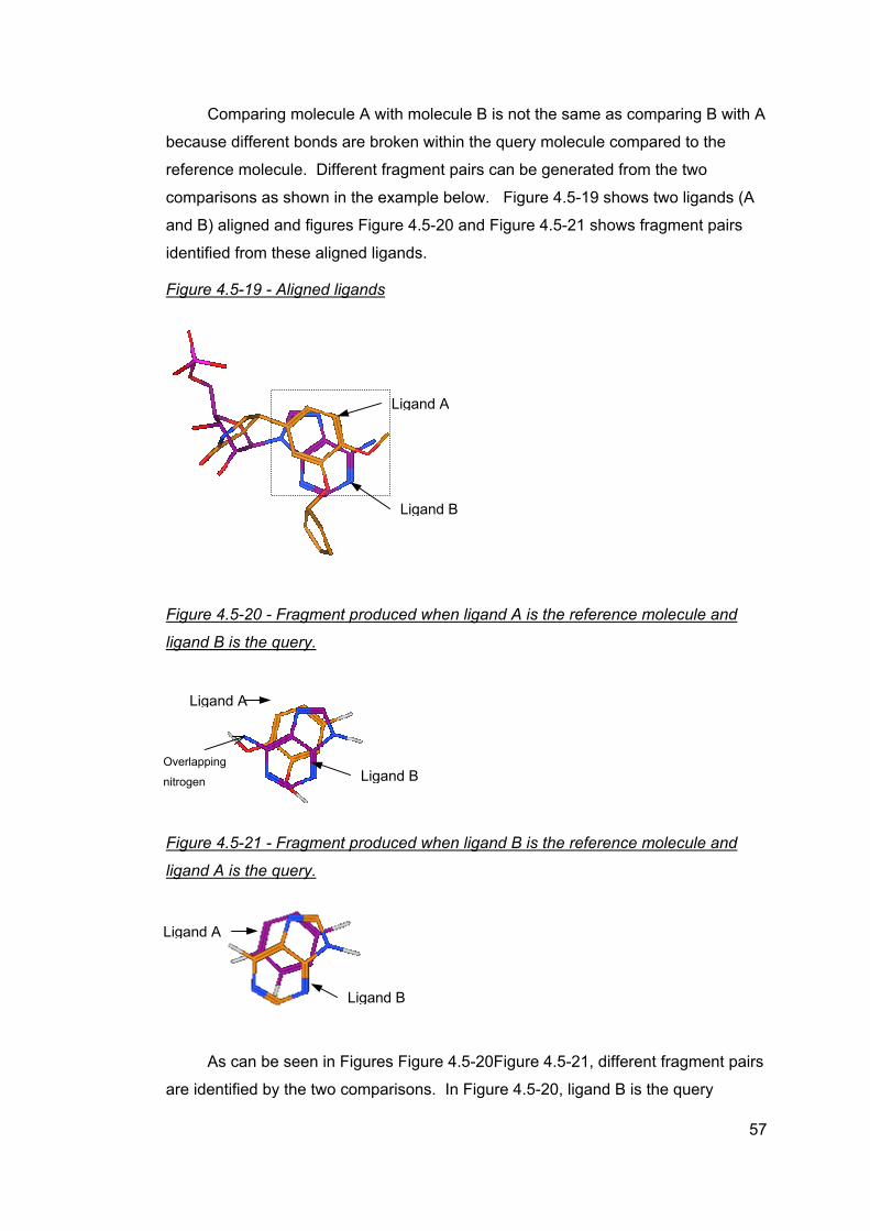
Comparing molecule A with molecule B is not the same as comparing B with A
because different bonds are broken within the query molecule compared to the
reference molecule. Different fragment pairs can be generated from the two
comparisons as shown in the example below. Figure 4.5-19 shows two ligands (A
and B) aligned and figures Figure 4.5-20 and Figure 4.5-21 shows fragment pairs
identified from these aligned ligands.
Figure 4.5-19 - Aligned ligands
Ligand A
Ligand B
Figure 4.5-20 - Fragment produced when ligand A is the reference molecule and
ligand B is the query.
Ligand A
Overlapping
nitrogen Ligand B
Figure 4.5-21 - Fragment produced when ligand B is the reference molecule and
ligand A is the query.
A
LigandLigand B
As can be seen in Figures Figure 4.5-20Figure 4.5-21, different fragment pairs
are identified by the two comparisons. In Figure 4.5-20, ligand B is the query
57
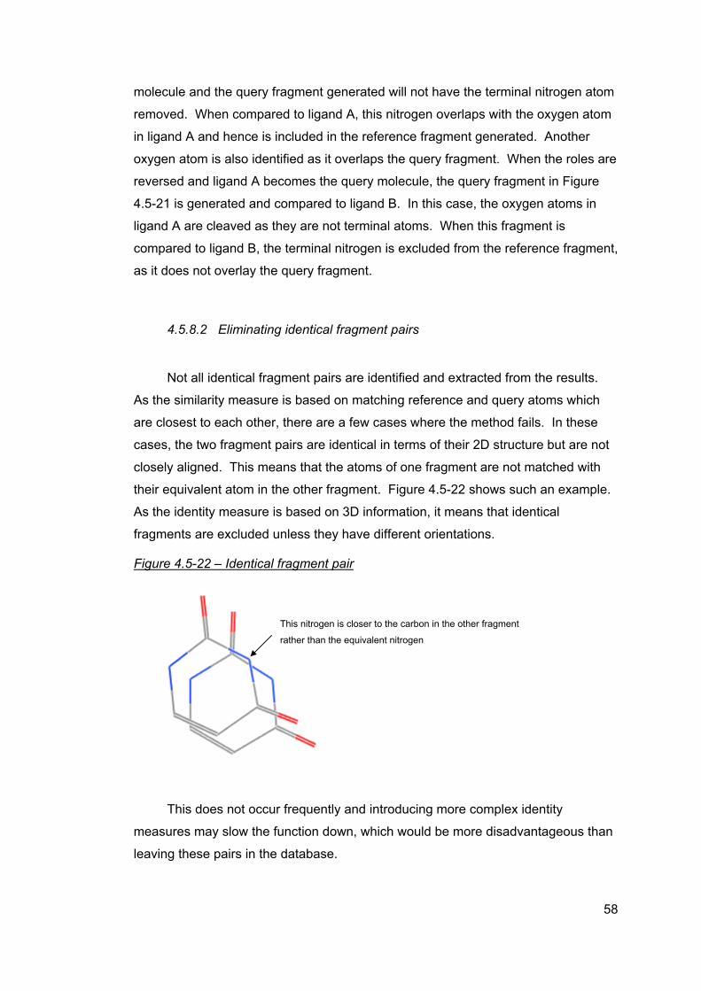
molecule and the query fragment generated will not have the terminal nitrogen atom
removed. When compared to ligand A, this nitrogen overlaps with the oxygen atom
in ligand A and hence is included in the reference fragment generated. Another
oxygen atom is also identified as it overlaps the query fragment. When the roles are
reversed and ligand A becomes the query molecule, the query fragment in Figure
4.5-21 is generated and compared to ligand B. In this case, the oxygen atoms in
ligand A are cleaved as they are not terminal atoms. When this fragment is
compared to ligand B, the terminal nitrogen is excluded from the reference fragment,
as it does not overlay the query fragment.
4.5.8.2 Eliminating identical fragment pairs
Not all identical fragment pairs are identified and extracted from the results.
As the similarity measure is based on matching reference and query atoms which
are closest to each other, there are a few cases where the method fails. In these
cases, the two fragment pairs are identical in terms of their 2D structure but are not
closely aligned. This means that the atoms of one fragment are not matched with
their equivalent atom in the other fragment. Figure 4.5-22 shows such an example.
As the identity measure is based on 3D information, it means that identical
fragments are excluded unless they have different orientations.
Figure 4.5-22 – Identical fragment pair
This nitrogen is closer to the carbon in the other fragment
rather than the equivalent nitrogen
This does not occur frequently and introducing more complex identity
measures may slow the function down, which would be more disadvantageous than
leaving these pairs in the database.
58

4.5.8.3 Extracting the correct ligand
The ligands, along with their protein, are extracted from the PDB file of
protein-ligand complexes from the PDB. Unfortunately the PDB file does not contain
bond order information, or atom geometry, only connectivity data. Therefore when
the ligands are extracted, the bond orders and hence geometry of the atoms within
the molecule need to be determined. Bond orders within the ligand are determined
based on the distance between two atoms. This approximation can result in some
bonds being assigned the wrong bond order. As hydrogen atoms are not seen in
an X-ray structure then they cannot be used to help establish correct bond order.
The ligand in Figure 4.5-23 (part of the HIV1 dataset) has been depicted incorrectly
with the double bond attached to the ring rather than within it.
Figure 4.5-23 Incorrect ligand structure drawn
Wrongly depicted
bond order
Without 2D structural information (the element type and geometry of each
atom) then it is not possible to determine computationally whether the ligand has
been drawn correctly. The ligands could be visually checked to ensure the correct
conformation has been drawn but this is obviously time consuming especially for
large ligand datasets.
Currently this problem has not been resolved but there are avenues that can
be explored. Geometry information is available for structures within the PDB. This
information is contained within files separate to the main PDB file. This information
would then need to be extracted for each ligand using the unique code assigned to
59
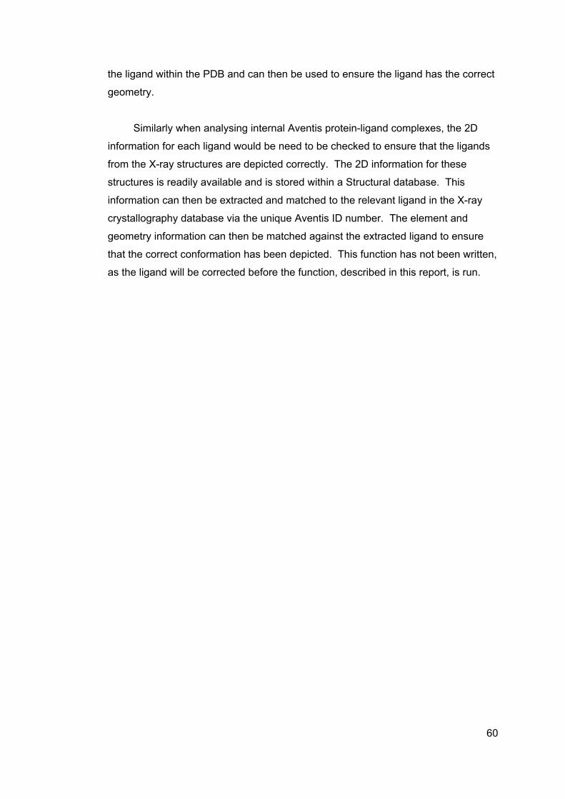
the ligand within the PDB and can then be used to ensure the ligand has the correct
geometry.
Similarly when analysing internal Aventis protein-ligand complexes, the 2D
information for each ligand would be need to be checked to ensure that the ligands
from the X-ray structures are depicted correctly. The 2D information for these
structures is readily available and is stored within a Structural database. This
information can then be extracted and matched to the relevant ligand in the X-ray
crystallography database via the unique Aventis ID number. The element and
geometry information can then be matched against the extracted ligand to ensure
that the correct conformation has been depicted. This function has not been written,
as the ligand will be corrected before the function, described in this report, is run.
60
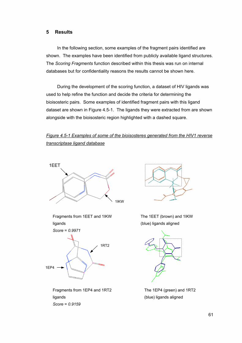
5 Results
In the following section, some examples of the fragment pairs identified are
shown. The examples have been identified from publicly available ligand structures.
The Scoring Fragments function described within this thesis was run on internal
databases but for confidentiality reasons the results cannot be shown here.
During the development of the scoring function, a dataset of HIV ligands was
used to help refine the function and decide the criteria for determining the
bioisosteric pairs. Some examples of identified fragment pairs with this ligand
dataset are shown in Figure 4.5-1. The ligands they were extracted from are shown
alongside with the bioisosteric region highlighted with a dashed square.
Figure 4.5-1 Examples of some of the bioisosteres generated from the HIV1 reverse
transcriptase ligand database
W
Fragments from 1EET and 1IKW
ligands
Score = 0.9971
1EP4
Fragments from 1EP4 and 1RT2
ligands
Score = 0.9159
1IK
1EET
The 1EET (brown) and 1IKW
(blue) ligands aligned
1RT2
The 1EP4 (green) and 1RT2
(blue) ligands aligned
61
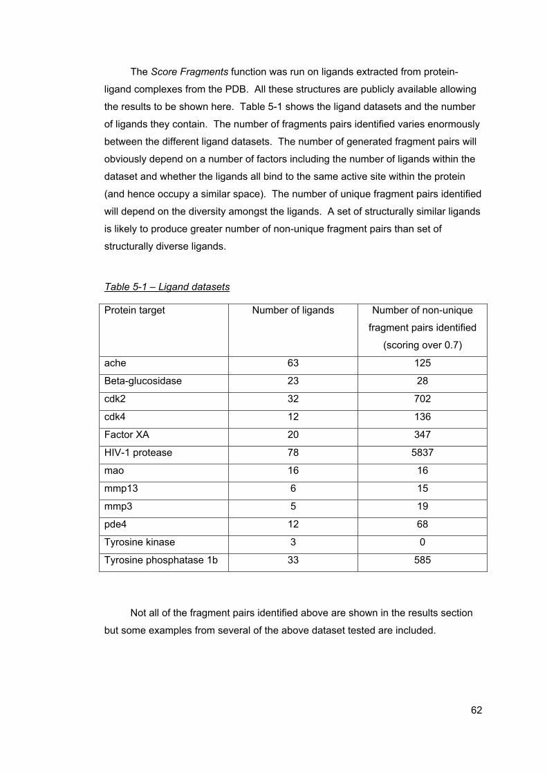
The Score Fragments function was run on ligands extracted from protein-
ligand complexes from the PDB. All these structures are publicly available allowing
the results to be shown here. Table 5-1 shows the ligand datasets and the number
of ligands they contain. The number of fragments pairs identified varies enormously
between the different ligand datasets. The number of generated fragment pairs will
obviously depend on a number of factors including the number of ligands within the
dataset and whether the ligands all bind to the same active site within the protein
(and hence occupy a similar space). The number of unique fragment pairs identified
will depend on the diversity amongst the ligands. A set of structurally similar ligands
is likely to produce greater number of non-unique fragment pairs than set of
structurally diverse ligands.
Table 5-1 – Ligand datasets
Protein target Number of ligands Number of non-unique
fragment pairs identified
(scoring over 0.7)
ache 63 125
Beta-glucosidase 23 28
cdk2 32 702
cdk4 12 136
Factor XA 20 347
HIV-1 protease 78 5837
mao 16 16
mmp13 6 15
mmp3 5 19
pde4 12 68
Tyrosine kinase 3 0
Tyrosine phosphatase 1b 33 585
Not all of the fragment pairs identified above are shown in the results section
but some examples from several of the above dataset tested are included.
62
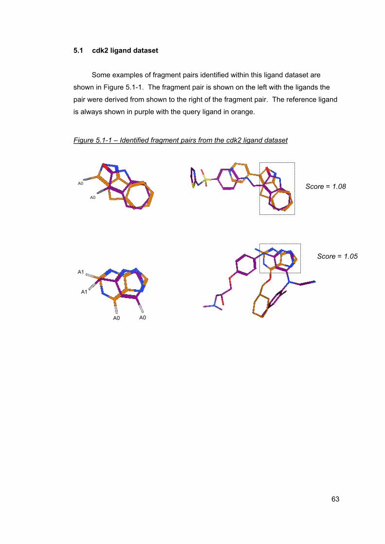
5.1 cdk2 ligand dataset
Some examples of fragment pairs identified within this ligand dataset are
shown in Figure 5.1-1. The fragment pair is shown on the left with the ligands the
pair were derived from shown to the right of the fragment pair. The reference ligand
is always shown in purple with the query ligand in orange.
Figure 5.1-1 – Identified fragment pairs from the cdk2 ligand dataset
Score = 1.08
Score = 1.05
63
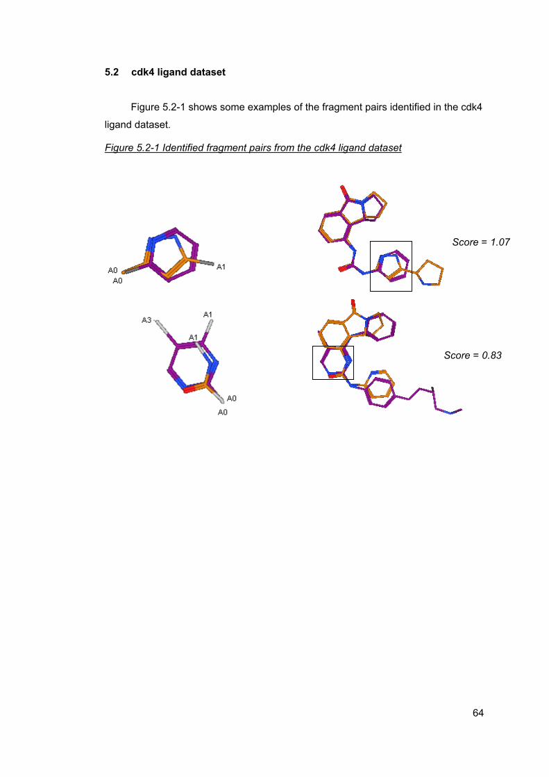
5.2 cdk4 ligand dataset
Figure 5.2-1 shows some examples of the fragment pairs identified in the cdk4
ligand dataset.
Figure 5.2-1 Identified fragment pairs from the cdk4 ligand dataset
Score = 1.07
Score = 0.83
64
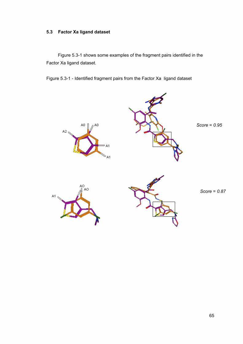
5.3 Factor Xa ligand dataset
Figure 5.3-1 shows some examples of the fragment pairs identified in the
Factor Xa ligand dataset.
Figure 5.3-1 - Identified fragment pairs from the Factor Xa ligand dataset
Score = 0.95
Score = 0.87
65
6 Conclusions
The concept of identifying potential bioisosteres via structural data has been
shown to work as fragment pairs that occupy the same space within a pair of aligned
ligands have been identified (as seen in the Results chapter above). This means
that potential bioisosteres can be identified using X-Ray crystallography data as a
start point. These structures may not have explicit activity data associated with
them but rather activity has been derived indirectly from analysing their binding
mode.
The Scoring Fragments function can be applied to different sets of ligands as
demonstrated in the Results chapter where the function was tested against different
ligand dataset sets. The function was also run against both external and internal
ligand datasets and fragment pairs were identified in both cases.
As the Scoring Fragments function identifies potential bioisosteres in terms of
the space they occupy within the protein, the resulting fragment pairs may not
necessarily be involved in intermolecular binding but can have other roles such as
being part of the scaffold region or a linker. Databases such as IsoStar can only
provide information regarding functional groups which make the same or similar
intermolecular interactions. Identifying potential bioisosteres within other regions
could be important as they could have an impact on other properties without having
a detrimental effect on the binding affinity (as they are not involved in making
intermolecular bonds).
The Scoring Fragments function will analyse a ligand data set quickly, a ligand
dataset of 81 compounds was analysed in less than 5 minutes with approximately
1500 fragment pairs produced. The time taken for the program to run obviously
increases with the size of the ligand dataset but more importantly it increases with
complexity of the ligands. If the ligands contain long chain sections (comprising of
single bonds) then the Splitting Molecules function will generate a large number of
fragments, all of which need to be compared to the reference molecule. This said, it
could be possible for the Scoring Fragments function to be run as an online program
which is run when necessary ensuring the most up-to-date results are obtained.
The function could be rerun when a new ligand, or ligands, is entered into the ligand
dataset. If the function can be run when needed then this may enable the user to
66
choose different settings, such as specify which cutoff values are incorporated, to
refine the output for their needs.
The Scoring Fragments function is generating information which would then be
investigated further. The next step is to determine whether the identified fragment
pairs are useful bioisosteres. As previously discussed, it is assumed that because
all the ligands within a dataset bind to the same target protein they have the same
biological activity therefore replacement of one fragment for the other within a pair
should not alter the activity significantly. It is not possible to investigate whether a
fragment replacement alters the degree of activity, as activity data is not readily
available in publicly available structures (i.e. those from the PDB). What needs to
be established is whether replacing one fragment with the other alters other
properties such as solubility, toxicity or ADME properties. This will determine
whether the bioisosteres would be useful to be incorporated during the lead
generation, or optimisation, stage. The main aim is to identify bioisosteres which will
improve the properties of a lead compound. If the bioisostere does not have any
effect then there is nothing to be gained from incorporating them into a lead
compound. Similarly if the bioisostere causes a reduction of a desirable property
then this is also not a valuable bioisostere.
As property data is not readily available from PDB structures, then is it not
possible to easily determine this from the datasets where the ligands were extracted
from the PDB (as shown in the Results section). Instead the fragment pairs would
have to be compared against a database of molecules where property data for these
molecules was more easily available.
For each unique fragment pair, the database would be searched to find pairs
of molecules that only differ from one another by that fragment pair. If they differ in
other regions outside this fragment pair then they cannot be used to establish what
effect, if any, this fragment replacement would have as any change noted could not
be attributed to just the fragment pair replacement. The molecules do not have to
have activity against the same protein target, as the ligands the fragment pair was
identified from, because the property data being looked at, such as solubility or
toxicity, is not dependant on the molecule’s activity towards a particular protein
target.
67

Once pairs of molecules have been identified for a particular fragment pair, the
property data for the two molecules would be compared to establish which property,
or properties, if any, are altered between the two molecules and the ∆Pi will then be
determined (where Pi is the altered property). These ∆Pi values can then be used in
further statistical analysis to determine whether the change is significant. Also the
statistical analysis can be used to compare bioisosteric pairs. The change in
property can then be attributed to the replacement of one fragment for the other. It
may be the case that no property is significantly changed between the molecule
pairs. In this case the bioisosteres would not be deemed useful, as the replacement
would provide no improvement during a lead generation stage. It is important to note
that this validation process is dependant on the content of the molecule database
and is reliant on data being available for molecules which only differ by the fragment
pair being investigated. If only a small number of molecule pairs are identified for a
particular fragment pair then the statistical data may not be sufficient to draw any
firm conclusions.
If the fragment pair is found to cause an alteration in the properties between
the two molecules being compared then this pair, they can be flagged as being a
potentially interesting bioisostere. These biosiosteres can then be saved into a
separate database. It is important to record the replacement this relates to – i.e.
which fragment is being replaced with the other fragment in order to see the change.
Several factors could be taken into consideration when analysing the data from the
fragment pairs, such as:
- The magnitude of change of the particular property (∆Pi)
- The distribution of the magnitude between molecule pairs– do some molecule
pairs exhibit a greater change in property than others?
- The number of the molecule pairs the data has been derived from
- The distribution of alteration within the molecule pair dataset – did all the
molecule pairs exhibit a change in the particular property or only a subset.
If the replacement causes a change in a certain property in only a subset of
the molecule pairs then it may be interesting to try and determine why this is
occurring. Can a common feature amongst the molecules in the subset be identified
which is not found in the molecules where no change is observed? These would
only be observations at this stage because it would not be possible to confirm this
68
without further investigation.
If pairs of molecules cannot be identified which only differ in terms of a
particular fragment pair then is it obviously not possible to establish what effect this
replacement would have. These fragment pairs should not be discarded because it
may not mean that the replacement does not have an effect but that appropriate
molecules have not been synthesised and tested yet. These fragment pairs could
be investigated again at a later date when the database is populated with more
molecules. Indeed, these fragment pairs may prove to be especially interesting if
they have not been considered as useful bioisosteres before.
This project represents the beginning stages of a process in which the ultimate
aim is to identify bioisosteric replacements which will give medicinal chemists ideas
on how to improve and optimise a lead compound.
69
Bibliography Alberts B, Bray D, Johnson A, Lewis J, Raff M, Roberts K & Walter P (1998)
“Binding Site of a Protein” http://www.accessexcellence.org/AB/GG/prot_Bindg.html
Access Excellence @ National Health Museum [Accessed 14th May]
Allen F; Davies J, Galloy J, Johnson O, Kennard O, Macrae C, Mitchell E, Mitchell
G, Smith J & Watson D (1991) “The Development of Versions 3 and 4 of the
Cambridge Structural Database System” J. Chem. Inf. Comput. Sci 31, 187-204
Andrews P & Tintelnot M (1990) “Intermolecular Forces and Molecular Binding” In:
Ramsden C (eds) Comprehensive Medicinal Chemistry pp321-348 UK Pergamin
Press plc
Berman H, Westbrook J, Feng Z, Gililand G, Bhat T, Weissig H, Shindyalov I and
Bourne P (2000) “The Protein Data Bank” Nuc. Acids Res. 28(1) 235-242
BIOSTER (2004a) “BIOSTER” www.accelrys.com/chem_db/bioster.html Accelrys
[Online] [Accessed 13th April]
BIOSTER (2004b) “Bioster Database – from Accelrys”
http://cds.dl.ac.uk/cds/datasets/orgchem/isis/trial/bioster.html Chemical Database
Service [Online] 8th April [Accessed 1st May]
Bleasdale J, Ogg D, Palazuk B, Jacob C, Swanson M, Wang X, Thompson D,
Cornadi R, Mattews W, Laborde A, Stuchly C, Heijbel A, Bergdahl K, Bannow C,
Smith C, Svensson C, Lijebris C, Schostarez H, May P, Stevens & Larsen S (2001)
“Small Molecule Peptidomimetics Containing a Novel Phosphotyrosine Bioisostere
Inhibit Protein Tyrosine Phophatase 1B and Augment Insulin Action” Biochemistry
40(19) 5642-5654
Bohl M, Dunbar J, Gifford E, Heritage T, Wild D, Willett P & Wilton D (2002)
“Scaffold Searching: Automated Identification of Similar Ring Systems for the
Design of Combinatorial Libraries” Quant. Struct.-Act. Relat. 21, 590-597
Bruno I, Cole J, Lommerse R, Rowland R, Taylor R & Verdonk M (1997) “IsoStar: A
70
Library of Information about Nonbonded Interactions” J. Comp. Aid. Mol. Des. 11,
425-537
Bultinck P, Kuppens T, Girones X & Carbo-Dorca (2003) “Quantum Similarity
Superposition Algorithm (QSSA): A Consistent Scheme for Molecular Alignment and
Molecular Similarity Based on Quantum Chemistry” J. Chem. Inf. Comput. Sci. 43,
1143-1150
CCDC (2003) “Cambridge Crystallographic Data Centre 2003” Brochure CCDC
CSD (2004) “Cambridge Structural Database”
http://www.ccdc.cam.ac.uk/products/csd/information_content/ CCDC
[Online][Accessed 14th May]
Feher M & Schmitt J (2003) “Fuzzy Clustering as a Means of Selecting
Representative Conformers and Molecular Alignments” J. Chem. Inf. Comput. Sci.
43, 810-818
Gao J, Winslow S, Vander Velde D, Aube J & Borchardt R (2001) “Transport
Characteristics of Peptides and Peptidomimetics: II. Hydroxyethlamine bioisostere-
Containing Peptidomimetics as Substrates for the Oligopeptide Transporter and P-
glycoprotein in the Intestinal Mucosa” J. Peptide Res. 57, 361-373
Good A & Richards W (1993) “Rapid Evaluation of Shape Similarity using Gaussian
Functions” J. Chem. Inf. Comput. Sci 33, 112-116
Grant J, Gallardo M & Pickup B (1996) “A Fast Method of Molecular Shape
Comparison: A Simple Application of a Gaussian Description of Molecular Shape.” J. Com. Chem. 17 (14) 1653-1666
Gunther J, Bergner A, Hendlich M & Klebe G (2003) “Utilising Structural Knowledge
in Drug Design Strategies: Applications Using Relibase” J. Mol. Biol. 326, 621-636
Hendlich M, Bergner A, Gunther J & Klebe G (2003) “Relibase: Design and
Development of a Database for Comprehensive Analysis of Protein-Ligand
Interactions” J. Mol. Biol. 326, 607-620
71
Holliday J, Jelfs S & Willett P (2003) “Calculation of Intersubstituent Similarity Using
R-group descriptors” J. Chem. Inf. Comput. Sci. 43, 406-411
IsoStar (2003) “IsoStar”
http://www.ccdc.cam.ac.uk/products/knowledge_bases/isostar/ CCDC [Online]
[Accessed 29th April]
Klebe G, Mietzner T & Weber F (1994) “Different approaches towards an automatic
structural alignment of drug molecules: Applications to sterol mimics, thrombin and
thermolysin inhibitors” J. Comp. Aid. Mol. Des. 8, 751-778
Kotani K & Higashiura K (2002) “Rapid Evaluation of Molecular Shape Similarity
Using Pairwise Calculation of the Nearest Atomic Distances” J. Chem. Inf. Comput.
Sci. 42, 58-63
Leach A & Gillet V (2003) An Introduction to Chemoinformatics Kluwer Academic
Publishers Netherlands
Mederski W, Osswald M, Dorsch, Anzali S, Christadler M, Schmitges C & Wilm C
(1998) “2. Endothelin antagonists: Evaluation of 2,1,3-Benzothiadiazole as a
methylendioxyphenyl bioisoster” Bioorg. Med. Chem. Lett 8, 17-22
MOE Manual (2004) MOE
Patani G & LaVoie E (1996) “Bioisosterism: A Rational Approach in Drug Design”
Chem Rev 96, 3147-3176
PBD (2000) “Molecule of the month – HIV-1 Protease” Protein Data Bank [Online]
http://www.rcsb.org/pdb/molecules/pdb6_3.html [Accessed 29th April]
Relibase+ (2004) “Relibase+ - Easy searching of Protein-Ligand Complexes”
[Online] http://www.ccdc.cam.ac.uk/products/life_sciences/relibase/ [Accessed 7th
July]
RCSB PDB (2004) “Protein Data Bank” http://www.pdb.org/ RCSG. [Online]
[Accessed 29th April]
72
Rosenfield R, Swanson S, Meyer E, Carrell H & Murray-Rust (1984) “Mapping the
Atomic Environment of Functional Groups: Turning 3D Scatter Plots into Pseudo-
density Contours” J. Mol. Graphics 20, 43-46
Schneider G, Neidhart W, Giller T & Schmid G (1999) “”Scaffold-Hopping” by
Topological Pharmacophore Search: A Contribution to Virtual Screening” Angew.
Chem. Int. Ed 38 (19) 2894-2896
Sheridan R (2002) “The Most Common Chemical Replacements in Drug-Like
Compounds” J. Chem. Inf. Comput. Sci 42, 103-108
Showell G & Mills J (2003) “Chemistry Challenges in Lead Optimization: Silicon
Isosteres in Drug Discovery” Drug Discovery Today 8(12) 551-556
Stryer L (1988) “Biochemistry” New York W.H. Freeman and Company
Uddin M, Praveen Rao P & Knaus E (2003) “Design and Synthesis of Novel
Celecoxib Analogues as Selective Cyclooxgenase-2 (COX-2) Inhibitors:
Replacement of the Sulfonamide Pharmacophore by a Sulfonylazide Bioisostere”
Bioorg. Med. Chem. 11, 5273-5280
Verdonk M, Cole J & Taylor R (1999) “SuperStar: A Knowledge-based Approach for
Identifying Interaction Sites in Proteins” J. Mol. Bio. 289, 1093-1108
Verdonk M, Cole J, Watson P, Gillet V & Willett P (2001) “SuperStar: Improved
Knowledge-based Interaction Fields for Protein Binding Sites” J. Mol. Bio. 307, 841-
859
Vyvyan J (2004) “Structure Activity Relationships” Western Washington University
http://www.chem.wwu.edu/vyvyan/C425cSAR.ppt [Online] [April 29th]
Watson P, Willett P, Gillet V & Verdonk M (2001) “Calculating the Knowledge-based
Similarity of Functional Groups using Crystallographic Data” J. Comp. Aid. Mol. Des.
15,835-857
73
74
Yuen P, Schelkun R, Szoke B & Tarczy-Hornoch K (1998) “Synthesis and Structure-
Activity Relationship of Substituted 1,2,3,4-tetrahydroisoquinolines as N-type
Calcium Channel Blockers” Bioorg. Med. Chem. Lett 8, 2415-2418