Embed Size (px)
Citation preview
IDENTIFICATION OF ACCIDENT BLACK-SPOTS IN 18 MICHIGAN FREEWAYS
USING GIS
Abdulla Ali, Ph.D., Student
Nishantha Bandara, Ph.D.,P.E., Assistant Professor
Susan Henson, M.S., Adjunct Professor
Department of Civil and Architectural Engineering
Lawrence Technological University
21000 W 10 Mile Rd, Southfield, MI 48075
ABSTRACT
Road accidents are one of the challenging problems affecting many parts of the world. The Michigan freeways are far
busier today than before. This led to the increase of traffic incidents due to several factors including human errors,
roadway deficiencies, environmental factors, vehicle factors, etc. A study conducted by Michigan Traffic Crash Facts
(MTCF) estimates an accident will happen every 44 minutes and every six hours a person will die on Michigan
roadways. The success of traffic safety and highway improvement programs depend on the analysis of accurate and
reliable traffic accident data. This study discusses the present traffic accident information on 18 freeways in Michigan.
It will also discuss the identification of high rate accident locations (black-spots) by using the Geographic Information
System (GIS) Software and safety deficient areas on the highway. This paper particularly discusses the use of two
statistical black-spot identification techniques, namely kernel density estimation (KDE) and the point density estimation (PDE). By comparing the two methods, it is found that both methods have resulted in reasonably different
sets of black-spots. However, KDE is more capable of pinpointing the black-spots than the PDE method.
KEYWORDS: Accident Black-Spots, Kernel Density Estimation (KDE), Point Density Estimation (PDE)
INTRODUCTION
There is an exponential increase in road problems, risks, and accidents in many nations worldwide. Timely
and accurate responses are required to avoid incidents of accidents and hazards on the road to guarantee a safe,
efficient, and faster travel experience. Road safety became a primary concern for road developers and those who are
concerned with public safety and well-being (Apparao, G., 2012). Black-spots are the areas of the road characterized
by high levels of accidents. Defining black-spots is significant for road safety and hazard elimination (Thakali, 2015).
Accordingly, the ability to determine black-spots can help with road network development in order to keep pace with the continuous increase in transportation and the risks and hazards associated with this increase. For the purpose of
this research, 18 freeway segments in Michigan were investigated to identify and evaluate accident black-spots.
Michigan is the eleventh biggest state in the USA by area, with a total land mass of 96,716 square miles. The
population in Michigan was approximately 9,909,877 in 2014 with a 0.3% percent change from 2010 (MTCF 2014).
According to MDOT (2015), the entire length of Michigan roads also increased from 110,656 miles in 1960 to 122,901
miles in 2010. The increase in road length accommodates the 1.8 percent increase in the number of vehicles and
vehicle mileage from the same period (MDOT 2015). The number of licensed drivers and total number of registered
vehicles on Michigan roads also increased by 0.4 percent (MTCF, 2014). In 2010, the total number of road accidents
was 282,075 with 868 fatalities, 51,672 seriously injured, and 229,535 slightly injured. There were 298,699 total
accidents statewide in 2014 with 0.9 deaths per 100 million miles of travel. As shown in figure 1, these results equate
to a 14.9 percent increase from 2010 (MTCF, 2014).

Figure 1. Total number of accidents statewide from 2010- 2014
This research analyzes accident and roadway environment data associated with respective road accidents.
The technique used for evaluation consists of three basic phases: identification, diagnosis, and remedy. The sequence
of phases identifies the accident causes and contribution factors, diagnoses safety problems at accident-prone
locations, and suggests appropriate countermeasures. In this study, Geographic Information Systems (GIS) is utilized
to detect road accident black-spots on Michigan expressways. Two methods of identifying road accident black-spots were used: kernel density estimation (KDE) and point density estimation (PDE).
LITERATURE REVIEW
Traffic, roadway configuration, weather conditions, vehicle characteristics, human perception, etc. are the
main reasons for road incidents (Shinar, 2007). In uncertain road environments, anticipating and quantifying the time
and locations where accidents have a high probability of occurring is not easy. However, identifying locations that
experience black-spots can pinpoint areas that may contribute to a higher accident risk compared to other similar
locations. Additionally, avoiding major danger and fatalities in the future (Molla, 2014) is another benefit. Black-spots
could be an indication of hazardous-prone areas in the freeway network which experience a high volume of accidents.
Sometimes ineffective methods can lead to identifying a safe location as dangerous (false positive) or a dangerous
location as safe (false negative). Some methods of black-spots identification fail to include minor injuries, and
accidents causing property damage only (Washington, 2014). Hazards on the road resulting in accidents, crimes, and fatalities are a major threat to public safety (Kuo, 2013).
Research conducted on the identification of black-spots is very limited; however, several methods have been
proposed and implemented in this field. Some of these methods depend on counting or rating accidents using a
negative binominal technique which is not accurate in estimating accidents that change from a year-to-year (Thakali,
2015). This approach can be exhaustive and give inaccurate data (Kuo, 2013). One method to identify black-spots
includes dividing the road section into constant lengths, where the total length is divided into 300-, 500-, and 1,000-
meter road sections. However, this method is inaccurate because the section length is constant where accidents within
each section may not be related to each other. Further, the method tends to overlook dangerous locations in which the
section lengths should be long enough to cover all continuous accidents that appear to be related to one another (Mitra,
2008). The Conventional Method section lengths vary from country to country as shown Table 1.
Table 1. The Conventional Method to Identify Highway Black-Spots
Country Section Length Frequency
Australia Fairly short At least 3 casualty accidents in 5 years
England 300 meters 12 accidents in 3 years
Germany 300 meters 8 accidents in 3 years
Norway 100 meters 4 accidents in 3 years
Portugal 200 meters 5 accidents in 3 years
Thailand (DOH) Variable At least 3 accidents in 1 years
282,075284,049
273,891
289,061
298,699
270,000
275,000
280,000
285,000
290,000
295,000
300,000
2010 2011 2012 2013 2014
No.
of
Acc
iden
ts
Year
Trend of Road Accidents From 2010-2014

The Michigan Department of Transportation and other state Departments of Transportation (DOT)
identifying black-spots to ensure that money allotted to identify black-spots is well spent. Properly identified black-
spots help ensure the safety of drivers by reducing the frequency of accidents and their severity (MDOT 2015). The
kernel density estimation (KDE) is one of the well-known and frequently used methods in identifying black-spots,
calculating accident intensity, and studying the spatial pattern of the accident. There are multiple kernel functions such
as uniform, normal, and quartic. There are other methods that examine and evaluate risk relative to location using clustering models such as the “K-mean clustering, Moran’s I Index, nearest neighborhood hierarchical (NNH)
clustering, and Getis-Ord Gi statistics” (Thakali, 2015).
Point density estimation was used to produce an event zone (black-spot) and a surface by using the weights
and density of points in an area (Jones, 2008). In a study conducted by Thakali in 2015 that aimed to define black-
spots in Hennepin County, Minnesota, two geostatistical methods were compared: KDE and kriging. Hennepin County
supplied historical accident data (2003 to 2007) collected at different times during the day for this study. Table 2
below compares the black-spot identification methods listed above and other potential methods. The method and goal
of each method are listed (Ansari, 2014).
Table 2. Different Methods for Black-Spot Identification in GIS
Summary of the Selected Methods The Point Density tool identifies the density of point features located in a specified neighborhood. If a point
feature has a value other than none, the tool incorporates that value into the density calculation. For example, a
neighborhood of 10 pixels containing points weighted as 8 would be calculated by counting each point 8 times to
obtain the value for that neighborhood (Jones, 2008). The number of points located within a neighborhood is divided
by the area of the neighborhood. This result, or density, is assigned to a grid cell. In other words, point density
calculates a volume per unit area of a neighborhood around each output cell. The point density tool creates the event
zone characterized by a surface based on the weights and the concentration of points in an area (ArcGIS, 2005).
Figure 2. PDE Method to calculate the density of the population around each output cell
The Kernel Density tool depends on stretching the known amount of population associated with each point
out from the location of this point as a way to calculate the density of features in a neighborhood around those features.
The produced surfaces surrounding every point in kernel density are based on a quadratic shape with the maximum
value at the center of the surface and narrowing down to zero at the search radius distance. The following steps are
used to determine the default search radius, or “bandwidth” (ArcGIS, 2016):
1. Calculate the mean center of all input points keeping in mind that all calculations are weighted by the values in that field.
2. Calculate the distance from the (weighted) mean center for all point.
3. Calculate the (weighted) median of these distances, Dm.
4. Determine the (weighted) Standard Distance, SD.
5. Calculate the bandwidth using the following formula:
Method Goal
Kernel density For smoothing effect within radius and cell size
Point Density Calculates a volume per unit area of a neighborhood around each output cell
Line Density Calculates a volume per unit area for radius of the cell size
IDW Interpolation Classifying within max and min value
Kriging For assuming spatial variation of attribute
Spline For smoothing effect
Morans I For present of the cluster of similar values
Geties-Ord Gi* For separating the high and low values of clusters

Search Radius = 0.9 × min(SD, √1
ln(2)×𝐷𝑚) ∗ 𝑛-0.2
Where “min” means that the smallest value of the two resulting options will only be considered (ArcGIS, 2016).
Figure 3. KDE spreads the known amount of the population for each point out from the point location
Both the PDE and KDE methods use points as input and produce raster grids as output. The raster grids are made up
of grid cells that contain the calculated density values.
METHODOLOGY
The proposed methodology in this study illustrates how GIS can be used to identify black-spot locations and
implement analysis of the black-spots. This study uses Arcmap10.3 GIS for Network Accident Analysis and includes
two main parts: data collection and analysis of contributing factors related to the accidents. The data for this study was obtained from the present traffic accident information from the State of Michigan. The study also discusses the
identification of high rate accident locations and safety deficient areas on the highway by using GIS Software. The
traffic accident data were obtained from MTCF website for the years (2010-2014). For this study, a step-by-step
method was adopted:
1. Collect data from MTCF for high number of accidents that happened on freeways in Michigan for the years
2010-2014.
2. Collect GPS information from MTCF and convert the coordinate system to NAD_1983, the datum used by
the State of Michigan transportation framework.
3. Export, merge, and save data obtained for each year from 2010 to 2014 as a shapefile (see figure 4).
4. Determine black-spots using the two spatial analysis tools: Point Density Estimation (PDE) and Kernel
Density Estimation (KDE). Evaluate and compare the results of these tools to determine which method is
better suited to find black-spots in this and future research.
3.1 Data Analysis Sample accident data from freeway M-31 was used in this study as shown in table 3. This data includes the
following elements: road name, road condition, speed limit, weather, light condition, type of accident, and x and y
coordinates.
Table 3. Shown Data (Road Condition, Weather, and X, Y Coordinates)
No Road
Name
Road
Condition
Speed
Limit
Weather Light Accident
Type
GPS X
Coordinate
GPS Y
Coordinate
1 M-31 Snowy 55 mph Snow/blowing Snow Dark Unlighted Single Motor -85.0757 45.3591
2 M-31 Icy 70 mph Snow/blowing Snow Dark Unlighted Angle -86.2111 43.09664
3 M-31 Snowy 35 mph Snow/blowing Snow Dark Lighted Angle -86.0806 42.78333
4 M-31 Icy 70 mph Snow/blowing Snow Daylight Angle -86.3111 41.91413
5 M-31 Slushy 55 mph Snow/blowing Snow Daylight Angle -85.3434 45.25483
6 M-31 Snowy 45 mph Snow/blowing Snow Dark Lighted Angle -85.646 44.72294
(1)

Figure 4. Major accident locations in 18 freeway Michigan
A total of 370,016 accidents occurred from 2010 to 2014. The following road and weather conditions were
noted relative to the number of accidents:
1. Road conditions:
a. Dry – 237,132 accidents b. Snowy, slushy, and icy – 64,616 accidents
c. Others – 68,268 accidents
2. Weather conditions:
a. Clear weather – 188,020 accidents
b. Rain – 38,502 accidents
c. Snow/blowing snow – 46,447 accidents
d. Others – 97,047 accidents
Figure 5 shows that more than two-third of the accidents happened in dry road conditions. Similarly, more than half
of the accidents happened during clear weather conditions.
Figure 5. Percentage of accidents based on road condition and weather conditions

3.2 Kernel Density Estimation (KDE) Method Kernel Density Estimation (KDE) is an ideal method to calculate if the significance of a point is affected
more by known points than by those farther away. The kernel radius should preferably be small and insignificant
enough to be representative of local variation within the region. The scale should be compatible with the size of the region and big enough to seize multiple point locations within the kernel radius (Thakali, 2015). The following
equation was used to calculate kernel density:
𝑓(𝑥, 𝑦) = ∑ (1
𝑛×2×𝜋ℎ2×𝑊𝑖×𝐾(
𝑑𝑖
ℎ))
𝑛
𝑖=1
Where 𝑓(𝑥, 𝑦) is the density estimate at the location (x,y); 𝑛 is the number of observations; ℎ is the bandwidth; 𝐾 is
the kernel function and 𝑑𝑖 is the distance between the location (x, y) and 𝑖 the observation; and 𝑊𝑖 is the density of
the observation. For the accident count, 𝑊𝑖 is a unit, whereas this may vary when we consider different weights for
different accidents.
3.3 Point Density Estimation (PDE) Method
𝜌𝑞 =∑𝜌𝑖 ϵ𝐶(𝑞,𝑟)
𝜋𝑟2 (3)
Where 𝜌𝑞 the density at a location q, 𝐶(𝑞, 𝑟)is a circular search area centered on q with a radius of r, and 𝜌𝑖 are the
values of points contained within the search area (Jones, 2008). The Point Density Estimation is a density tool found
within the ArcGIS Spatial Analyst toolset. Point Density Estimation was used to determine the region of blackspot
occurrence. Point density estimation has the ability to pinpoint the co-occurrence of points within the neighborhood of each one of these points. This technique depends on the concept that a surface is a set of points and by using the
density of points within a search radius, as well as the weighted value of these points, it is possible to determine the
value of each output raster cell.
Method Comparison Both the kernel density and point density estimation methods are used to find different types of densities such
as the density of houses, crimes, accidents, or roads. Both methods employ a radius variable. The major impact of
using a larger radius is that the density can be determined using a larger number of points. However, those points can
be farther away from the resulting calculated raster cell. Figure 6 shows a summary of the methodology used for this research.
Figure 6. Comparison between PDE and KDE
These two density estimation methods were used to estimate the accident density of the 18 freeways in the
State of Michigan. A summary detailing each method was offered in Sections 3.2 and 3.3.
3.4 Black-Spots Selection Criteria When applying the KDE and PDE methods to generate accident density maps for the 18 freeways, a grid cell
size of 1887.297561m x 1887.297561m was enforced. Both methods also incorporated a radius of 400 meters. By incorporating a standard cell size and radius, both methods produced output containing the same number of cells. This
allowed for easier comparison between the two methods.
After running each method, each grid cell was assigned a value. The higher the value, the higher the accident
density, or accident risk. Cells are classified into a specific range or class depending upon the cell value. Each class
PDE KDE
(2)

was assigned a specific color and manually assigned a letter value or level. These levels are categorized as risk level
A, risk level B, and so on. Black-spots are then determined as the level having the highest density of accidents, in this
case, level F. As shown in the resulting density maps (figure 7), the locations of black-spots appear to be similar for
both methods.
Figure 7. KDE (left) and PDE (right) results for 2010-2014 accident data
RESULTS AND DISCUSSIONS
The density results were classified into six classes or levels. The six levels are listed in ascending order of
risk. Each of these levels represents approximately 10% of the total map area. These levels are represented by color-
coded areas that show accident density. The areas in blue indicate higher risk. The kernel density and point density
estimation methods show that the areas known to be accident-prone are condensed in the 18 freeways used in this
research. The areas having higher traffic interaction (urban areas) have more traffic and safety problems. The risk
level decreases when the highways spread outwardly from the heart of the urban areas.
Figures 8-12 show PDE and KDE results per year. Some differences are noted between the two methods
relative to year. A group of hotspots were selected that allowed careful investigation and comparisons. The selection
of black-spots was not based on a certain criteria and varied one study to another. The basis for selection was choosing
a set of regions with higher safety risks. In this study, the KDE quartic method was utilized. In this method, the top

risk level was chosen from the formerly referred to sets of risk levels. Statistically, cut-off values, such as the mean,
can be identified based on the estimated accidents within the area used.
Figure 8. PDE (left) and KDE (right) results for 2010
Figure 9. PDE (left) and KDE (right) results for 2011

Figure 10. PDE (left) and KDE (right) results for 2012
Figure 11. PDE (left) and KDE (right) results for 2013
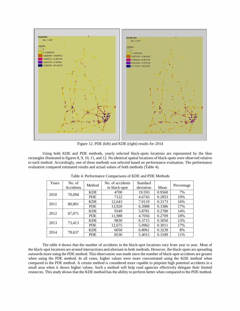
Figure 12. PDE (left) and KDE (right) results for 2014
Using both KDE and PDE methods, yearly selected black-spots locations are represented by the blue
rectangles illustrated in figures 8, 9, 10, 11, and 12. No identical spatial locations of black-spots were observed relative
to each method. Accordingly, one of these methods was selected based on performance evaluation. The performance
evaluation compared estimated results and actual values of both methods (Table 4).
Table 4. Performance Comparisons of KDE and PDE Methods
Years No. of
Accidents Method
No. of accidents
in black-spot
Standard
deviation
Mean Percentage
2010 70,094 KDE 4700 19.593 0.9560 7%
PDE 7122 4.6743 0.2853 10%
2011 80,801 KDE 12,643 7.0119 0.3173 16%
PDE 13,920 6.3988 0.3386 17%
2012 67,071 KDE 9349 5.8781 0.2780 14%
PDE 11,988 4.7056 0.2709 18%
2013 73,413 KDE 9830 6.3715 0.3050 13%
PDE 12,675 5.0962 0.3011 17%
2014 78,637 KDE 6050 6.8061 0.3239 8%
PDE 8530 5.4015 0.3189 11%
The table 4 shows that the number of accidents in the black-spot locations vary from year to year. Most of
the black-spot locations are around intersections and alternate in both methods. However, the black-spots are spreading
outwards more using the PDE method. This observation was made since the number of black-spot accidents are greater when using the PDE method. In all cases, higher values were more concentrated using the KDE method when
compared to the PDE method. A certain method is considered more capable to pinpoint high potential accidents in a
small area when it shows higher values. Such a method will help road agencies effectively delegate their limited
resources. This study shows that the KDE method has the ability to perform better when compared to the PDE method.
At the same time, the KDE method can be used in the future to better locate black-spots as compared with other
statistical modeling approaches.
CONCLUSION
The two geostatistical methods evaluated in this analysis are called Kernel Density Estimation (KDE) and
Point Density Estimation (PDE). PDE is comparable to KDE in such it weighs the surrounding weighted values to
derive an estimated density for a measured site. KDE is one of the well-known spatial statistical methods that proved
to be very powerful in managing regional black-spot analysis. Both PDE and KDE methods were used previously in
the study of road safety. However, KDE was applied more frequently than PDE in investigating black spots for areas
that are likely to cause a health problem or areas that have high levels of crime. In this research study, KDE is presented
as a promising alternative that is characterized by its ability to handle spatially autocorrelated datasets that can be used
successfully to pinpoint black spots. The two methods were compared in a case study for identifying accident black-
spots using the road network of the State of Michigan. Historical accident data from 2010 to 2014 was used. After applying both methods, the KDE results were more concentrated and considered more desirable for black-spot
determination then the PDE results.
REFERENCES
Ansari, & Kale, 2014. Methods for crime analysis using GIS; International Journal of Scientific & Engineering Research 5(12): 1330-1336.
Apparao, G., Mallikarjunareddy, P., & Gopala, R, 2012. Identification of accident black spots for national highway
using GIS, International Journal of Scientific and Technology Research, 2(2): 154-157.
ArcGIS. 2005. Density calculations. ESRI.com. http://webhelp.esri.com/arcgisdesktop/9.1/index.cfm?
TopicName=Density%20calculations
ArcGIS, 2016. How kernel density works. ArcGIS. http://pro.arcgis.com/en/pro-app/tool-reference/spatial-
analyst/how-kernel-density-works.htm
Jones, Purves, Clough, & Joho, 2008. Modelling vague places with knowledge from the Web, International Journal
of Geographical Information Science 22(10): 1045-1065.
Kuo, P., Lord, D., & Walden, T., 2013. Using geographical information systems to organize police patrol routes
effectively by grouping hotspots of crash and crime data, Journal of Transport Geography 30, 138-148. MDOT, 2015. Michigan department of transportation, Michigan.Gov. http://www.michigan.gov/mdot/
Michigan Traffic Crash Facts: A summary of traffic crashes on Michigan roadways, 2014. Department of
Transportation.
Mitra, S., 2008. Enhancing road traffic safety: A GIS based methodology to identify potential areas of improvement,
California Polytechnic State University, San Luis Obispo, CA.
Molla, Mohammad, M., & Matthew, 2014. Geostatistical approach to detect traffic accident hotspots and clusters in
North Dakota; Upper Great Plains Transportation Institute.
Shinar, D., 2007. Traffic safety and human behavior, Elsevier, Oxford, England, Emerald Group Publishing Limited.
Thakali, 2015. Identification of crash hotspots using kernel density estimation and kriging methods: A comparison,
Springerlink.com.
Washingtona, H., 2014. Applying quantile regression for modeling equivalent property damage only crashes to identify accident blackspots, Accident; analysis and prevention 66:136–146.