Identification in Structural Models Linking Energy and Corn Cash Markets

Veronica F. Pozo Assistant Professor

Department of Applied Economics Utah State University

veronica.pozo@usu.edu

Vladimir Bejan Assistant Professor

Department of Economics Seattle University

bejanv@seattleu.edu

Selected Paper prepared for presentation at the 2016 Agricultural & Applied Economics

Association Annual Meeting, Boston, Massachusetts, July 31-August 2

Copyright 2016 by Veronica F. Pozo and Vladimir Bejan. All rights reserved. Readers may make verbatim copies of this document for non-commercial purposes by any means, provided that this copyright notice appears on all such copies.

1

Introduction

Following the increased reliance on biofuels in industrialized economies, particularly in the United

States after the passage of the Energy Policy Act of 2005, the question of how changes affecting

oil and ethanol markets are transmitted to agricultural commodities markets has been a subject of

major concern in the literature (Sierra and Zilberman, 2013). To answer this question, researchers

have typically applied reduce-form vector autoregressive (VAR) or vector error correction (VEC)

models to time series data to establish causal links between these markets. However, according to

Baumeister and Kilian (2014), most part of this literature is based on atheoretical models that are

incapable of establishing such links in the data. That is, they lack of any economic interpretation

because reduced-form errors are mutually correlated (Kilian and Vigfusson, 2011). Therefore,

claims about how changes in energy markets impact grain commodity markets, and vice versa, are

not well founded.

To deal with this problem, researchers have turned to structural VAR and VEC models.

The estimation of these models requires additional identifying assumptions that must be motivated

based on economic theory. The assumptions most commonly employed for identification are

imposed by using exclusion, sign, short-run, long-run, and covariance restrictions. However, in

the case of agricultural markets, such restrictions are hard to justify a priori.

The objective of this study is to determine causal links between energy and corn

commodity markets using structural VAR and VEC models. More specifically, to quantify how

shocks to crude oil and ethanol markets are transmitted to corn cash prices, and vice versa. Here,

the identification problem is solved by implementing a novel approach proposed by Rigobon

(2003), which is based on the heteroskedasticity of structural shocks. An advantage of using this

approach is that it does not rely on a specific ordering of variables in the model. Identification is

achieved by recognizing regimes of high and low volatility. Thus, this method estimates, rather

than imposes, the pattern of contemporaneous correlations between price variables used in this

analysis. This study adds to the literature by illustrating the use of this approach where regimes

of high and low volatility are identified using information obtained from historical price volatility

data.

Understanding the links between oil, ethanol and corn cash markets is critical not only for

producers and processors as they make production, marketing, and risk management decisions, but

also for policy makers as they design policies that may be intended to support the ethanol industry.

2

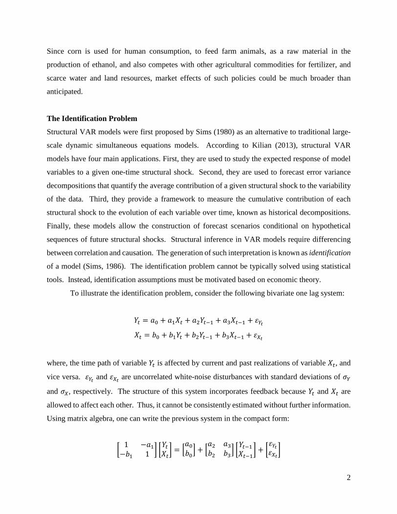
Since corn is used for human consumption, to feed farm animals, as a raw material in the

production of ethanol, and also competes with other agricultural commodities for fertilizer, and

scarce water and land resources, market effects of such policies could be much broader than

anticipated.

The Identification Problem

Structural VAR models were first proposed by Sims (1980) as an alternative to traditional large-

scale dynamic simultaneous equations models. According to Kilian (2013), structural VAR

models have four main applications. First, they are used to study the expected response of model

variables to a given one-time structural shock. Second, they are used to forecast error variance

decompositions that quantify the average contribution of a given structural shock to the variability

of the data. Third, they provide a framework to measure the cumulative contribution of each

structural shock to the evolution of each variable over time, known as historical decompositions.

Finally, these models allow the construction of forecast scenarios conditional on hypothetical

sequences of future structural shocks. Structural inference in VAR models require differencing

between correlation and causation. The generation of such interpretation is known as identification

of a model (Sims, 1986). The identification problem cannot be typically solved using statistical

tools. Instead, identification assumptions must be motivated based on economic theory.

To illustrate the identification problem, consider the following bivariate one lag system:

𝑌𝑌𝑡𝑡 = 𝑎𝑎0 + 𝑎𝑎1𝑋𝑋𝑡𝑡 + 𝑎𝑎2𝑌𝑌𝑡𝑡−1 + 𝑎𝑎3𝑋𝑋𝑡𝑡−1 + 𝜀𝜀𝑌𝑌𝑡𝑡

𝑋𝑋𝑡𝑡 = 𝑏𝑏0 + 𝑏𝑏1𝑌𝑌𝑡𝑡 + 𝑏𝑏2𝑌𝑌𝑡𝑡−1 + 𝑏𝑏3𝑋𝑋𝑡𝑡−1 + 𝜀𝜀𝑋𝑋𝑡𝑡

where, the time path of variable 𝑌𝑌𝑡𝑡 is affected by current and past realizations of variable 𝑋𝑋𝑡𝑡, and

vice versa. 𝜀𝜀𝑌𝑌𝑡𝑡 and 𝜀𝜀𝑋𝑋𝑡𝑡 are uncorrelated white-noise disturbances with standard deviations of 𝜎𝜎𝑌𝑌

and 𝜎𝜎𝑋𝑋, respectively. The structure of this system incorporates feedback because 𝑌𝑌𝑡𝑡 and 𝑋𝑋𝑡𝑡 are

allowed to affect each other. Thus, it cannot be consistently estimated without further information.

Using matrix algebra, one can write the previous system in the compact form:

� 1 −𝑎𝑎1−𝑏𝑏1 1 � �𝑌𝑌𝑡𝑡𝑋𝑋𝑡𝑡

� = �𝑎𝑎0𝑏𝑏0� + �

𝑎𝑎2 𝑎𝑎3𝑏𝑏2 𝑏𝑏3� �

𝑌𝑌𝑡𝑡−1𝑋𝑋𝑡𝑡−1

� + �𝜀𝜀𝑌𝑌𝑡𝑡𝜀𝜀𝑋𝑋𝑡𝑡�

3

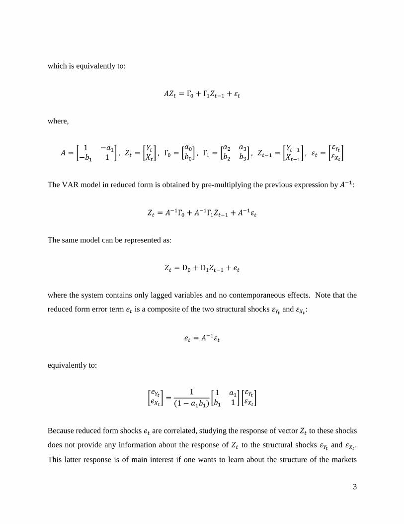
which is equivalently to:

𝐴𝐴𝑍𝑍𝑡𝑡 = Γ0 + Γ1𝑍𝑍𝑡𝑡−1 + 𝜀𝜀𝑡𝑡

where,

𝐴𝐴 = � 1 −𝑎𝑎1−𝑏𝑏1 1 � , 𝑍𝑍𝑡𝑡 = �𝑌𝑌𝑡𝑡𝑋𝑋𝑡𝑡

� , Γ0 = �𝑎𝑎0𝑏𝑏0� , Γ1 = �

𝑎𝑎2 𝑎𝑎3𝑏𝑏2 𝑏𝑏3� , 𝑍𝑍𝑡𝑡−1 = �𝑌𝑌𝑡𝑡−1𝑋𝑋𝑡𝑡−1

� , 𝜀𝜀𝑡𝑡 = �𝜀𝜀𝑌𝑌𝑡𝑡𝜀𝜀𝑋𝑋𝑡𝑡�

The VAR model in reduced form is obtained by pre-multiplying the previous expression by 𝐴𝐴−1:

𝑍𝑍𝑡𝑡 = 𝐴𝐴−1Γ0 + 𝐴𝐴−1Γ1𝑍𝑍𝑡𝑡−1 + 𝐴𝐴−1𝜀𝜀𝑡𝑡

The same model can be represented as:

𝑍𝑍𝑡𝑡 = D0 + D1𝑍𝑍𝑡𝑡−1 + 𝑒𝑒𝑡𝑡

where the system contains only lagged variables and no contemporaneous effects. Note that the

reduced form error term 𝑒𝑒𝑡𝑡 is a composite of the two structural shocks 𝜀𝜀𝑌𝑌𝑡𝑡 and 𝜀𝜀𝑋𝑋𝑡𝑡:

𝑒𝑒𝑡𝑡 = 𝐴𝐴−1𝜀𝜀𝑡𝑡

equivalently to:

�𝑒𝑒𝑌𝑌𝑡𝑡𝑒𝑒𝑋𝑋𝑡𝑡� =

1(1 − 𝑎𝑎1𝑏𝑏1)

� 1 𝑎𝑎1𝑏𝑏1 1 � �

𝜀𝜀𝑌𝑌𝑡𝑡𝜀𝜀𝑋𝑋𝑡𝑡�

Because reduced form shocks 𝑒𝑒𝑡𝑡 are correlated, studying the response of vector 𝑍𝑍𝑡𝑡 to these shocks

does not provide any information about the response of 𝑍𝑍𝑡𝑡 to the structural shocks 𝜀𝜀𝑌𝑌𝑡𝑡 and 𝜀𝜀𝑋𝑋𝑡𝑡.

This latter response is of main interest if one wants to learn about the structure of the markets

4

under study (Kilian, 2013). To reconstruct 𝜀𝜀𝑌𝑌𝑡𝑡 and 𝜀𝜀𝑋𝑋𝑡𝑡 it is necessary to recover the elements of

𝐴𝐴−1 from consistent estimates of the reduced-form parameters. To do so, one needs to impose

identification assumptions or restrictions based on economic theory. Such restrictions may take

the form of exclusion restrictions, sign restrictions, or recursive restrictions (i.e., Cholesky

decomposition). However, in some cases, such as in the analysis of price dynamics between

agricultural and related markets, it is not possible to justify these restrictions a priori. In such

cases, researchers have to implement more complex identification techniques.

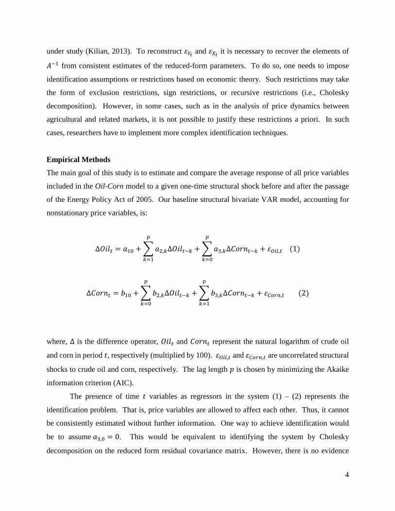
Empirical Methods

The main goal of this study is to estimate and compare the average response of all price variables

included in the Oil-Corn model to a given one-time structural shock before and after the passage

of the Energy Policy Act of 2005. Our baseline structural bivariate VAR model, accounting for

nonstationary price variables, is:

∆𝑂𝑂𝑂𝑂𝑂𝑂𝑡𝑡 = 𝑎𝑎10 + �𝑎𝑎2,𝑘𝑘∆𝑂𝑂𝑂𝑂𝑂𝑂𝑡𝑡−𝑘𝑘

𝑝𝑝

𝑘𝑘=1

+ �𝑎𝑎3,𝑘𝑘∆𝐶𝐶𝐶𝐶𝐶𝐶𝐶𝐶𝑡𝑡−𝑘𝑘

𝑝𝑝

𝑘𝑘=0

+ 𝜀𝜀𝑂𝑂𝑂𝑂𝑂𝑂,𝑡𝑡 (1)

∆𝐶𝐶𝐶𝐶𝐶𝐶𝐶𝐶𝑡𝑡 = 𝑏𝑏10 + �𝑏𝑏2,𝑘𝑘∆𝑂𝑂𝑂𝑂𝑂𝑂𝑡𝑡−𝑘𝑘

𝑝𝑝

𝑘𝑘=0

+ �𝑏𝑏3,𝑘𝑘∆𝐶𝐶𝐶𝐶𝐶𝐶𝐶𝐶𝑡𝑡−𝑘𝑘

𝑝𝑝

𝑘𝑘=1

+ 𝜀𝜀𝐶𝐶𝐶𝐶𝐶𝐶𝐶𝐶,𝑡𝑡 (2)

where, ∆ is the difference operator, 𝑂𝑂𝑂𝑂𝑂𝑂𝑡𝑡 and 𝐶𝐶𝐶𝐶𝐶𝐶𝐶𝐶𝑡𝑡 represent the natural logarithm of crude oil

and corn in period 𝑡𝑡, respectively (multiplied by 100). 𝜀𝜀𝑂𝑂𝑂𝑂𝑂𝑂,𝑡𝑡 and 𝜀𝜀𝐶𝐶𝐶𝐶𝐶𝐶𝐶𝐶,𝑡𝑡 are uncorrelated structural

shocks to crude oil and corn, respectively. The lag length 𝑝𝑝 is chosen by minimizing the Akaike

information criterion (AIC).

The presence of time 𝑡𝑡 variables as regressors in the system (1) – (2) represents the

identification problem. That is, price variables are allowed to affect each other. Thus, it cannot

be consistently estimated without further information. One way to achieve identification would

be to assume 𝑎𝑎3,0 = 0. This would be equivalent to identifying the system by Cholesky

decomposition on the reduced form residual covariance matrix. However, there is no evidence

5

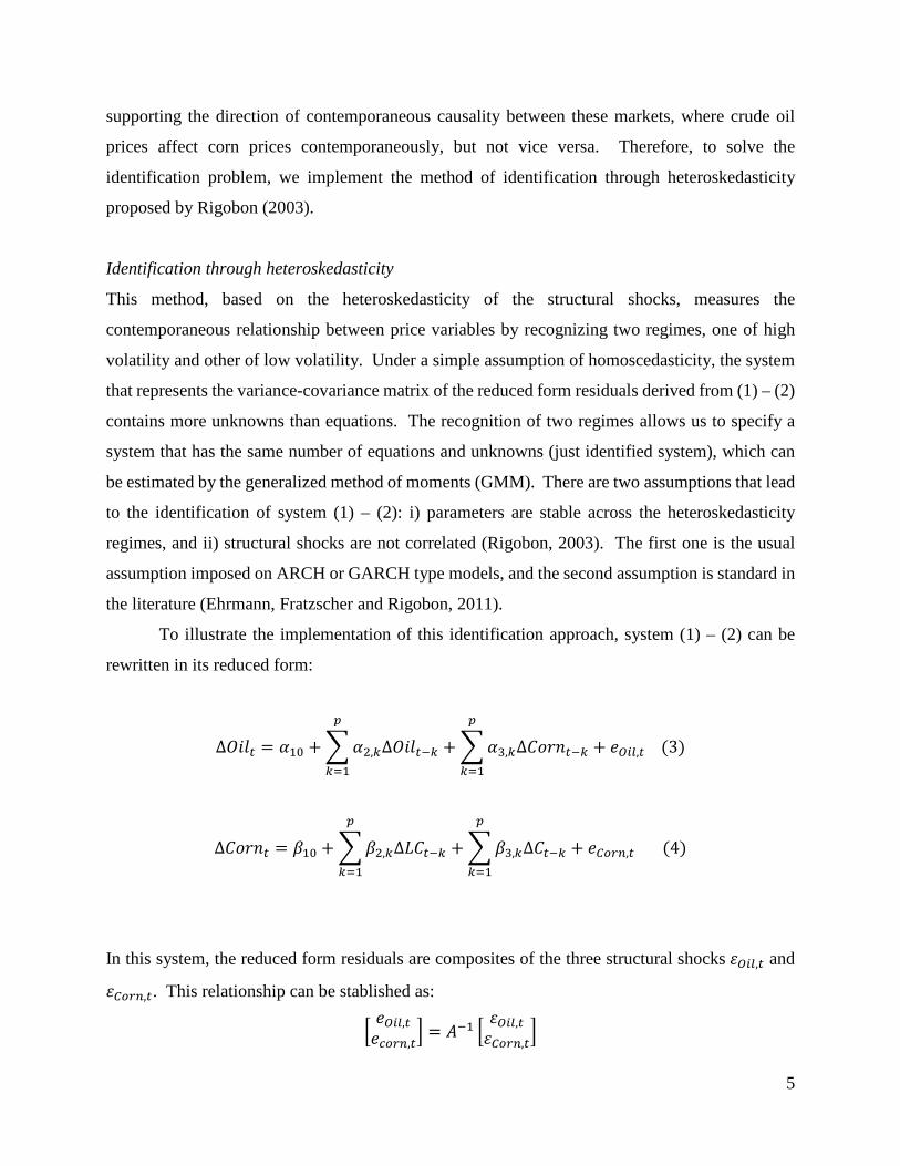
supporting the direction of contemporaneous causality between these markets, where crude oil

prices affect corn prices contemporaneously, but not vice versa. Therefore, to solve the

identification problem, we implement the method of identification through heteroskedasticity

proposed by Rigobon (2003).

Identification through heteroskedasticity

This method, based on the heteroskedasticity of the structural shocks, measures the

contemporaneous relationship between price variables by recognizing two regimes, one of high

volatility and other of low volatility. Under a simple assumption of homoscedasticity, the system

that represents the variance-covariance matrix of the reduced form residuals derived from (1) – (2)

contains more unknowns than equations. The recognition of two regimes allows us to specify a

system that has the same number of equations and unknowns (just identified system), which can

be estimated by the generalized method of moments (GMM). There are two assumptions that lead

to the identification of system (1) – (2): i) parameters are stable across the heteroskedasticity

regimes, and ii) structural shocks are not correlated (Rigobon, 2003). The first one is the usual

assumption imposed on ARCH or GARCH type models, and the second assumption is standard in

the literature (Ehrmann, Fratzscher and Rigobon, 2011).

To illustrate the implementation of this identification approach, system (1) – (2) can be

rewritten in its reduced form:

∆𝑂𝑂𝑂𝑂𝑂𝑂𝑡𝑡 = 𝛼𝛼10 + �𝛼𝛼2,𝑘𝑘∆𝑂𝑂𝑂𝑂𝑂𝑂𝑡𝑡−𝑘𝑘

𝑝𝑝

𝑘𝑘=1

+ �𝛼𝛼3,𝑘𝑘∆𝐶𝐶𝐶𝐶𝐶𝐶𝐶𝐶𝑡𝑡−𝑘𝑘

𝑝𝑝

𝑘𝑘=1

+ 𝑒𝑒𝑂𝑂𝑂𝑂𝑂𝑂,𝑡𝑡 (3)

∆𝐶𝐶𝐶𝐶𝐶𝐶𝐶𝐶𝑡𝑡 = 𝛽𝛽10 + �𝛽𝛽2,𝑘𝑘∆𝐿𝐿𝐶𝐶𝑡𝑡−𝑘𝑘

𝑝𝑝

𝑘𝑘=1

+ �𝛽𝛽3,𝑘𝑘∆𝐶𝐶𝑡𝑡−𝑘𝑘

𝑝𝑝

𝑘𝑘=1

+ 𝑒𝑒𝐶𝐶𝐶𝐶𝐶𝐶𝐶𝐶,𝑡𝑡 (4)

In this system, the reduced form residuals are composites of the three structural shocks 𝜀𝜀𝑂𝑂𝑂𝑂𝑂𝑂,𝑡𝑡 and

𝜀𝜀𝐶𝐶𝐶𝐶𝐶𝐶𝐶𝐶,𝑡𝑡. This relationship can be stablished as:

�𝑒𝑒𝑂𝑂𝑂𝑂𝑂𝑂,𝑡𝑡𝑒𝑒𝑐𝑐𝐶𝐶𝐶𝐶𝐶𝐶,𝑡𝑡

� = 𝐴𝐴−1 �𝜀𝜀𝑂𝑂𝑂𝑂𝑂𝑂,𝑡𝑡𝜀𝜀𝐶𝐶𝐶𝐶𝐶𝐶𝐶𝐶,𝑡𝑡

�

6

For simplicity, the 𝐵𝐵−1 matrix is defined as:1

𝐴𝐴−1 = � 1 𝛿𝛿1 𝛿𝛿2 1 �

Then, reduced form residuals can be specified as:

𝑒𝑒𝑂𝑂𝑂𝑂𝑂𝑂,𝑡𝑡 = 𝜀𝜀𝑂𝑂𝑂𝑂𝑂𝑂,𝑡𝑡 + 𝛿𝛿1 𝜀𝜀𝐶𝐶𝐶𝐶𝐶𝐶𝐶𝐶,𝑡𝑡

𝑒𝑒𝐶𝐶𝐶𝐶𝐶𝐶𝐶𝐶,𝑡𝑡 = 𝛿𝛿2 𝜀𝜀𝑂𝑂𝑂𝑂𝑂𝑂,𝑡𝑡 + 𝜀𝜀𝐶𝐶𝐶𝐶𝐶𝐶𝐶𝐶,𝑡𝑡

which shows how reduced form residuals are correlated. Thus, a one-time shock to any of the

variables included in a reduced form model will not tell us anything about the structure of their

underlying markets. To reconstruct 𝜀𝜀𝑂𝑂𝑂𝑂𝑂𝑂,𝑡𝑡 and 𝜀𝜀𝐶𝐶𝐶𝐶𝐶𝐶𝐶𝐶,𝑡𝑡 it is necessary to recover the elements of 𝐴𝐴−1

from consistent estimates of the reduced-form parameters. Under the assumptions of

homoscedasticity of the structural shocks, we have:

𝑣𝑣𝑎𝑎𝐶𝐶(𝑒𝑒𝑂𝑂𝑂𝑂𝑂𝑂) = 𝑣𝑣𝑎𝑎𝐶𝐶(𝜀𝜀𝑂𝑂𝑂𝑂𝑂𝑂) + 𝛿𝛿12𝑣𝑣𝑎𝑎𝐶𝐶(𝜀𝜀𝐶𝐶𝐶𝐶𝐶𝐶𝐶𝐶)

𝑐𝑐𝐶𝐶𝑣𝑣(𝑒𝑒𝑂𝑂𝑂𝑂𝑂𝑂, 𝑒𝑒𝐶𝐶𝐶𝐶𝐶𝐶𝐶𝐶) = 𝛿𝛿2𝑣𝑣𝑎𝑎𝐶𝐶(𝜀𝜀𝑂𝑂𝑂𝑂𝑂𝑂) + 𝛿𝛿1𝑣𝑣𝑎𝑎𝐶𝐶(𝜀𝜀𝐶𝐶𝐶𝐶𝐶𝐶𝐶𝐶)

𝑣𝑣𝑎𝑎𝐶𝐶(𝑒𝑒𝐶𝐶𝐶𝐶𝐶𝐶𝐶𝐶) = 𝛿𝛿22𝑣𝑣𝑎𝑎𝐶𝐶(𝜀𝜀𝑂𝑂𝑂𝑂𝑂𝑂) + 𝑣𝑣𝑎𝑎𝐶𝐶(𝜀𝜀𝐶𝐶𝐶𝐶𝐶𝐶𝐶𝐶)

This is a system of three equations and four unknowns, so it is not possible to estimate 𝐴𝐴−1 without

additional restrictions. Rigobon (2003) built on the logic that by recognizing two or more regimes

in the variances of the structural shocks, it is possible to identify the system with no further

restrictions. Letting the subscript 𝑂𝑂 = 1, 2 denote the regime, the following moment conditions

can be specified:

𝑣𝑣𝑎𝑎𝐶𝐶(𝑒𝑒𝑂𝑂𝑂𝑂𝑂𝑂𝑂𝑂 ) = 𝑣𝑣𝑎𝑎𝐶𝐶(𝜀𝜀𝑂𝑂𝑂𝑂𝑂𝑂𝑂𝑂 ) + 𝛿𝛿12𝑣𝑣𝑎𝑎𝐶𝐶(𝜀𝜀𝐶𝐶𝐶𝐶𝐶𝐶𝐶𝐶𝑂𝑂 )

𝑐𝑐𝐶𝐶𝑣𝑣(𝑒𝑒𝑂𝑂𝑂𝑂𝑂𝑂𝑂𝑂 , 𝑒𝑒𝐶𝐶𝐶𝐶𝐶𝐶𝐶𝐶𝑂𝑂 ) = 𝛿𝛿2𝑣𝑣𝑎𝑎𝐶𝐶(𝜀𝜀𝑂𝑂𝑂𝑂𝑂𝑂𝑂𝑂 ) + 𝛿𝛿1𝑣𝑣𝑎𝑎𝐶𝐶(𝜀𝜀𝐶𝐶𝐶𝐶𝐶𝐶𝐶𝐶𝑂𝑂 ) (5)

𝑣𝑣𝑎𝑎𝐶𝐶(𝑒𝑒𝐶𝐶𝐶𝐶𝐶𝐶𝐶𝐶𝑂𝑂 ) = 𝛿𝛿22𝑣𝑣𝑎𝑎𝐶𝐶(𝜀𝜀𝑂𝑂𝑂𝑂𝑂𝑂𝑂𝑂 ) + 𝑣𝑣𝑎𝑎𝐶𝐶(𝜀𝜀𝐶𝐶𝐶𝐶𝐶𝐶𝐶𝐶𝑂𝑂 )

1 It does not make a difference to divide each element of the matrix to the determinant of 𝐴𝐴 because it is a constant.

7

Here, there are six equations, and six unknowns: 𝛿𝛿1, 𝛿𝛿2, 𝑣𝑣𝑎𝑎𝐶𝐶(𝜀𝜀𝑂𝑂𝑂𝑂𝑂𝑂1 ), 𝑣𝑣𝑎𝑎𝐶𝐶(𝜀𝜀𝐶𝐶𝐶𝐶𝐶𝐶𝐶𝐶1 ), 𝑣𝑣𝑎𝑎𝐶𝐶(𝜀𝜀𝑂𝑂𝑂𝑂𝑂𝑂2 ) and

𝑣𝑣𝑎𝑎𝐶𝐶(𝜀𝜀𝐶𝐶𝐶𝐶𝐶𝐶𝐶𝐶2 ), indicating that the identification problem can be solved. The variance-covariance

matrix of the reduced form residuals can be computed for both regimes after estimating the reduced

form system (3) – (4).2 The coefficients in 𝐴𝐴−1 can be estimated by GMM using system (5) as

moment conditions, and standard errors can be obtained using the fixed-design wild bootstrap

(Goncalves and Kilian, 2004) with the Rademacher distribution as the pick distribution (Godfrey,

2009).

Before conducting the estimation procedure, the key question is how to identify regimes in

which the relative variances of the crude oil and corn market structural shocks changed over time.

Recent events affecting energy and corn markets represent a natural framework for regime

identification. This is because these events are associated with large and, in some cases, persistent

increases in volatility. In this study, regimes are identified by looking at the behavior of historical

volatilities. In this procedure, structural break tests are conducted in each historical volatility series

to find significant breaks. Thus, allowing us to define the regime windows systematically.

Because we are interested in finding all possible volatility regimes, we use the Bai and Perron

(2003) test to find multiple breaks.

Results and Discussion

In this study, three different models were estimated: two bivariate SVAR using crude oil and corn

prices for periods pre- and post-Energy Policy Act of 2005, and one trivariate SVEC model using

crude oil, corn and ethanol prices corresponding to the period after the implementation of the Act.

The data used for estimating these models are weekly Cushing, Oklahoma West Texas

Intermediate (WTI) crude oil spot prices FOB (dollars per barrel) and weekly Omaha, Nebraska

#2 yellow corn cash prices (dollars per bushel) from September 1997 to November 2015 (947

observations). The U.S. Energy Information Administration (EIA) is the source for WTI crude oil

cash price data and the Livestock Marketing Information Center for U.S. corn cash prices paid to

farmers. Weekly Iowa ethanol cash prices (dollars per gallon), from May 2006 to November 2015

(494 observations), were obtained from the Commodity Research Bureau (CRB). Moreover, to

2 The reduced form system (3) – (4) can be estimated by ordinary least squares (OLS).

8

estimate historical volatilities, daily cash price data for WTI crude oil, corn and ethanol were

collected from (CRB).

Following Baumeister and Kilian (2014), we split our sample in May 2006, when U.S.

policy toward ethanol changed with the implementation of the Energy Policy Act of 2005,

establishing a closer link between oil prices and corn prices. Therefore, model 1 (Oil-Corn) is

estimated using observations from September, 1997 to April, 2006; whereas models 2 (Oil-Corn)

and 3 (Oil-Ethanol-Corn) are estimated using observations from May 2006 to November 2015.

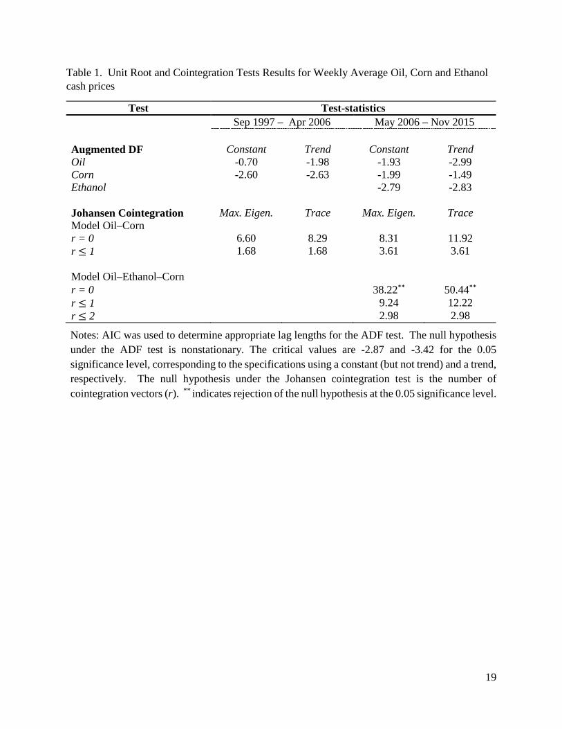
Table 1 presents results from the analysis of univariate time series properties, as well as

cointegration relationships among price variables in each model. To test for the presence of a unit

root in individual price series, we applied Augmented Dickey-Fuller (DF) tests. Results indicate

that all price series are nonstationary in every period.3 Furthermore, we tested for cointegration

among price variables using both specifications of the Johansen procedure (i.e., maximal

eigenvalue and trace statistic). Variables in the two bivariate models are not cointegrated.

Conversely, variables in the trivariate model are cointegrated with one cointegration relationship.

Thus confirming the appropriateness of estimating a SVEC model.

Measuring the Contemporaneous Relationship across Energy and Corn Prices

To identify contemporaneous coefficients in SVAR and SVEC models using the heteroskedasticity

of structural shocks, the first step is to identify high and low volatility regimes. This task was

performed by applying the Bai and Perron (2003) structural break test to weekly average historical

price volatilities of crude oil, corn and ethanol.4 This test allows to identify multiple breaks. We

allowed up to 5 breaks and used a trimming of at least 0.15, so each segment has a minimum of

15 observations. The best number of breaks was selected based on the Bayesian Information

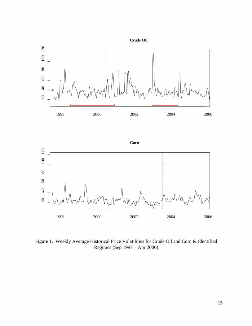
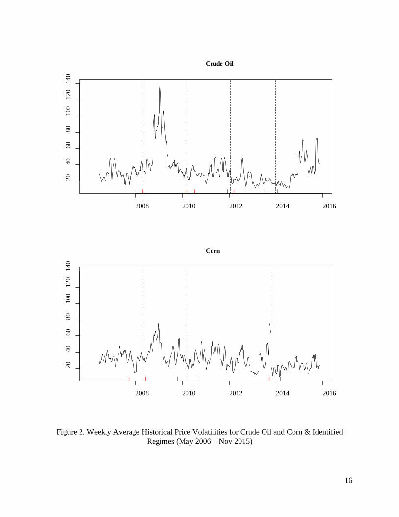
Criterion (BIC). Results are depicted in figures 1 and 2, corresponding to the pre- and post-Energy

Policy Act periods, respectively. The dotted lines in each plot indicates the break date, and the red

horizontal lines represent confidence bands for each break. In both figures, the price volatility in

the crude oil market presents larger variations than the price volatility in the corn market.

3 AIC was used to determine appropriate lag lengths for the Augmented DF test. 4 Daily historical volatilities (20-day) for each variable were first calculated using daily prices, and then averaged over the corresponding weekdays to obtain weekly historical volatilities. Daily historical volatilities were calculated following the procedure indicated by CRB. For more information on this procedure visit: http://www.crbtrader.com/support/options.asp

9

Looking at figure 1, the high volatility regime in the crude oil market ranges from 2000-

09-22 to 2008-03-08. This is not the case, however, for the corn market where the high volatility

regime is in period: 1997-09-18 – 1999-09-10. Conversely, the high volatility regimes for crude

oil and corn coincide in the post-Energy Policy Act period, as depicted in figure 2. Here, the high

volatility regime corresponds to period 2008-04-11 – 2010-02-26, which coincides with the market

recession in 2008. Moreover, the high volatility regime for the ethanol market (not depicted)

ranges from 2013-08-30 to 2015-11-05. Since it is not necessary to specify all the different

heteroskedasticity regimes to achieve identification, we define period 2000-09-22 to 2008-03-08

as the high volatility regime (regime 1), and all other observations as low volatility regime (regime

2), for the pre-Energy Policy Act period. Similarly, for the post-Energy Policy Act period, we

define period 2008-04-11 – 2010-02-26 as the high volatility regime (regime 1), and all other

observations as low volatility regime (regime 2).5

As the identification strategy delivers estimates of the variances of 𝜀𝜀𝑂𝑂𝑂𝑂𝑂𝑂 and 𝜀𝜀𝐶𝐶𝐶𝐶𝐶𝐶𝐶𝐶 in

models 1 and 2, and also 𝜀𝜀𝐸𝐸𝑡𝑡ℎ𝑎𝑎𝐶𝐶𝐶𝐶𝑂𝑂 in model 3, for both high and low volatility regimes, we can

formally verify that this choice of regimes is appropriate by comparing the magnitudes of the

structural shock variance estimates. That is, we can test whether the magnitudes of the variances

in the high volatility regime are systematically larger than the corresponding variances in the low

volatility regime, as discussed further below. The next step is the estimation procedure.

In the estimation procedure of models 1 and 2 (Oil-Corn), we follow four steps. First, the

reduced form VAR model is estimated as described in system (3) – (4).6 Based on AIC, these

models are estimated using 3 lags. Second, model residuals are used to construct the variance-

covariance matrix for each regime. Third, these variance-covariance matrices are used to create

the moment conditions that enter in the GMM estimation of the contemporaneous coefficients and

structural shocks variances, as described in system (5). Fourth, standard errors are computed using

a fixed-design wild bootstrap (500 replications). In the case of model 3 (Oil-Ethanol-Corn), we

follow the same steps with the only difference than instead of estimating a reduced form VAR we

5 Identification only requires that there are differences in the variances across the regimes we have selected. Therefore, it is not necessary that all variances in high volatility regimes are larger than those in low volatility regimes (Rigobon, 2003). 6 Results from the estimation of the reduced form VAR and VEC models are not presented but are available upon request. AIC was used to select the best number of lags.

10

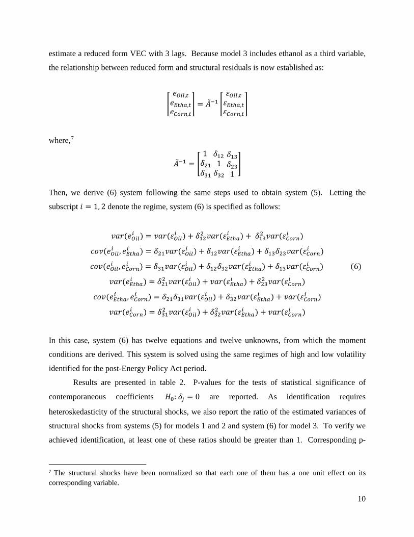
estimate a reduced form VEC with 3 lags. Because model 3 includes ethanol as a third variable,

the relationship between reduced form and structural residuals is now established as:

�𝑒𝑒𝑂𝑂𝑂𝑂𝑂𝑂,𝑡𝑡𝑒𝑒𝐸𝐸𝑡𝑡ℎ𝑎𝑎,𝑡𝑡𝑒𝑒𝐶𝐶𝐶𝐶𝐶𝐶𝐶𝐶,𝑡𝑡

� = �̃�𝐴−1 �𝜀𝜀𝑂𝑂𝑂𝑂𝑂𝑂,𝑡𝑡𝜀𝜀𝐸𝐸𝑡𝑡ℎ𝑎𝑎,𝑡𝑡𝜀𝜀𝐶𝐶𝐶𝐶𝐶𝐶𝐶𝐶,𝑡𝑡

�

where,7

�̃�𝐴−1 = �1 𝛿𝛿21 𝛿𝛿31

𝛿𝛿12 1 𝛿𝛿32

𝛿𝛿13𝛿𝛿231�

Then, we derive (6) system following the same steps used to obtain system (5). Letting the

subscript 𝑂𝑂 = 1, 2 denote the regime, system (6) is specified as follows:

𝑣𝑣𝑎𝑎𝐶𝐶(𝑒𝑒𝑂𝑂𝑂𝑂𝑂𝑂𝑂𝑂 ) = 𝑣𝑣𝑎𝑎𝐶𝐶(𝜀𝜀𝑂𝑂𝑂𝑂𝑂𝑂𝑂𝑂 ) + 𝛿𝛿122 𝑣𝑣𝑎𝑎𝐶𝐶(𝜀𝜀𝐸𝐸𝑡𝑡ℎ𝑎𝑎𝑂𝑂 ) + 𝛿𝛿132 𝑣𝑣𝑎𝑎𝐶𝐶(𝜀𝜀𝐶𝐶𝐶𝐶𝐶𝐶𝐶𝐶𝑂𝑂 )

𝑐𝑐𝐶𝐶𝑣𝑣(𝑒𝑒𝑂𝑂𝑂𝑂𝑂𝑂𝑂𝑂 , 𝑒𝑒𝐸𝐸𝑡𝑡ℎ𝑎𝑎𝑂𝑂 ) = 𝛿𝛿21𝑣𝑣𝑎𝑎𝐶𝐶(𝜀𝜀𝑂𝑂𝑂𝑂𝑂𝑂𝑂𝑂 ) + 𝛿𝛿12𝑣𝑣𝑎𝑎𝐶𝐶(𝜀𝜀𝐸𝐸𝑡𝑡ℎ𝑎𝑎𝑂𝑂 ) + 𝛿𝛿13𝛿𝛿23𝑣𝑣𝑎𝑎𝐶𝐶(𝜀𝜀𝐶𝐶𝐶𝐶𝐶𝐶𝐶𝐶𝑂𝑂 )

𝑐𝑐𝐶𝐶𝑣𝑣(𝑒𝑒𝑂𝑂𝑂𝑂𝑂𝑂𝑂𝑂 , 𝑒𝑒𝐶𝐶𝐶𝐶𝐶𝐶𝐶𝐶𝑂𝑂 ) = 𝛿𝛿31𝑣𝑣𝑎𝑎𝐶𝐶(𝜀𝜀𝑂𝑂𝑂𝑂𝑂𝑂𝑂𝑂 ) + 𝛿𝛿12𝛿𝛿32𝑣𝑣𝑎𝑎𝐶𝐶(𝜀𝜀𝐸𝐸𝑡𝑡ℎ𝑎𝑎𝑂𝑂 ) + 𝛿𝛿13𝑣𝑣𝑎𝑎𝐶𝐶(𝜀𝜀𝐶𝐶𝐶𝐶𝐶𝐶𝐶𝐶𝑂𝑂 ) (6)

𝑣𝑣𝑎𝑎𝐶𝐶(𝑒𝑒𝐸𝐸𝑡𝑡ℎ𝑎𝑎𝑂𝑂 ) = 𝛿𝛿212 𝑣𝑣𝑎𝑎𝐶𝐶(𝜀𝜀𝑂𝑂𝑂𝑂𝑂𝑂𝑂𝑂 ) + 𝑣𝑣𝑎𝑎𝐶𝐶(𝜀𝜀𝐸𝐸𝑡𝑡ℎ𝑎𝑎𝑂𝑂 ) + 𝛿𝛿232 𝑣𝑣𝑎𝑎𝐶𝐶(𝜀𝜀𝐶𝐶𝐶𝐶𝐶𝐶𝐶𝐶𝑂𝑂 )

𝑐𝑐𝐶𝐶𝑣𝑣(𝑒𝑒𝐸𝐸𝑡𝑡ℎ𝑎𝑎𝑂𝑂 , 𝑒𝑒𝐶𝐶𝐶𝐶𝐶𝐶𝐶𝐶𝑂𝑂 ) = 𝛿𝛿21𝛿𝛿31𝑣𝑣𝑎𝑎𝐶𝐶(𝜀𝜀𝑂𝑂𝑂𝑂𝑂𝑂𝑂𝑂 ) + 𝛿𝛿32𝑣𝑣𝑎𝑎𝐶𝐶(𝜀𝜀𝐸𝐸𝑡𝑡ℎ𝑎𝑎𝑂𝑂 ) + 𝑣𝑣𝑎𝑎𝐶𝐶(𝜀𝜀𝐶𝐶𝐶𝐶𝐶𝐶𝐶𝐶𝑂𝑂 )

𝑣𝑣𝑎𝑎𝐶𝐶(𝑒𝑒𝐶𝐶𝐶𝐶𝐶𝐶𝐶𝐶𝑂𝑂 ) = 𝛿𝛿312 𝑣𝑣𝑎𝑎𝐶𝐶(𝜀𝜀𝑂𝑂𝑂𝑂𝑂𝑂𝑂𝑂 ) + 𝛿𝛿322 𝑣𝑣𝑎𝑎𝐶𝐶(𝜀𝜀𝐸𝐸𝑡𝑡ℎ𝑎𝑎𝑂𝑂 ) + 𝑣𝑣𝑎𝑎𝐶𝐶(𝜀𝜀𝐶𝐶𝐶𝐶𝐶𝐶𝐶𝐶𝑂𝑂 )

In this case, system (6) has twelve equations and twelve unknowns, from which the moment

conditions are derived. This system is solved using the same regimes of high and low volatility

identified for the post-Energy Policy Act period.

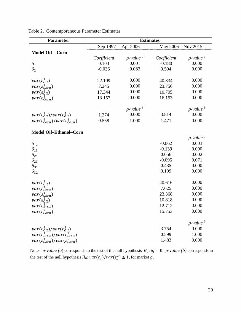
Results are presented in table 2. P-values for the tests of statistical significance of

contemporaneous coefficients 𝐻𝐻0: 𝛿𝛿𝑗𝑗 = 0 are reported. As identification requires

heteroskedasticity of the structural shocks, we also report the ratio of the estimated variances of

structural shocks from systems (5) for models 1 and 2 and system (6) for model 3. To verify we

achieved identification, at least one of these ratios should be greater than 1. Corresponding p-

7 The structural shocks have been normalized so that each one of them has a one unit effect on its corresponding variable.

11

values for the tests of the null hypotheses 𝐻𝐻0: 𝑣𝑣𝑎𝑎𝐶𝐶(𝜀𝜀𝑔𝑔1)/𝑣𝑣𝑎𝑎𝐶𝐶(𝜀𝜀𝑔𝑔2) ≤ 1, for market 𝑔𝑔 = 𝑂𝑂𝑂𝑂𝑂𝑂,𝐸𝐸𝑡𝑡ℎ𝑎𝑎

and 𝐶𝐶𝐶𝐶𝐶𝐶𝐶𝐶, are also included.

Results from the test of the ratios of variances of structural shocks in table 2 are used to

verify whether or not we were able to identify the systems. In all three models, the variance of

structural shocks for crude oil is larger in regime 1 compared to regime 2. For example, in model

2, the variance of the crude oil structural shock in regime 1 is almost 4 times larger than in regime

2 (40.8 vs. 10.7). Moreover, in model 1, the variance of the corn structural shock is smaller in

regime 1 than in regime 2. This is consistent with the expectations since high volatility regimes

did not coincide for both variables in model 1, and only the one for crude oil was selected. The

opposite occurs in model 2, since the periods of high volatility did coincide. Results from model

3 are similar to those in model 2. However, because the period of high volatility did not coincide

for ethanol, the variance of its structural shock is larger in regime 2 (7.6 vs. 12.7). The

bootstrapped p-values of the null hypotheses 𝐻𝐻0: 𝑣𝑣𝑎𝑎𝐶𝐶(𝜀𝜀𝑔𝑔1)/𝑣𝑣𝑎𝑎𝐶𝐶(𝜀𝜀𝑔𝑔2) ≤ 1 are 0 in all cases, except

when the high volatility regime corresponded to regime 2 (e.g., corn in model 1 and ethanol in

model 3). These results indicate that the large increase in the variances of the structural shocks in

the selected high volatility regimes is sufficient to achieve identification.

Continuing with table 2, we now focus on parameters estimates of contemporaneous

coefficients 𝛿𝛿𝑗𝑗 (corresponding to matrices 𝐴𝐴−1 for models 1 and 2, and matrix �̃�𝐴−1 for model 3).

Comparing the contemporaneous effects of oil prices in corn prices (𝛿𝛿2) between models 1 and 2,

this effect changes from being close to 0 on the period pre-Energy Policy Act, to 0.50 the period

after. Moreover, the contemporaneous effect of corn prices on crude oil prices (𝛿𝛿1) changes from

0.10 to -0.18 between both periods. Thus, suggesting that the causal links between these two

markets have changed after the passage of the Energy Policy Act. However, it does not necessarily

indicate that the passage of this Act is the sole reason for the observed change.

Focusing on the contemporaneous coefficients in model 3 (table 2), we can observe a

similar pattern as the one in model 2. For example, a 1 percent increase in the price of crude oil

leads to a 0.43 percent increase in the price of corn on the same week after the shock (𝛿𝛿31).

Interestingly, the contemporaneous effect of corn prices on ethanol prices is 0. That is, the estimate

of 𝛿𝛿23 is both economically and statistically insignificant. Although statistically significant, the

instantaneous effect of ethanol prices on crude oil prices, and vice versa are economically

12

insignificant – (𝛿𝛿12) and (𝛿𝛿21), respectively. Finally, the instantaneous effect of ethanol prices on

corn prices is positive and statistically significant (𝛿𝛿32).

Analysis of Impulse Response Functions

After identifying the contemporaneous effects in both systems, we are interested in evaluating the

total effect, contemporaneous and lagged, of a shock to each market on itself and on the other

variables included in the system. To do this, we focus on the calculation of cumulative impulse

response functions.

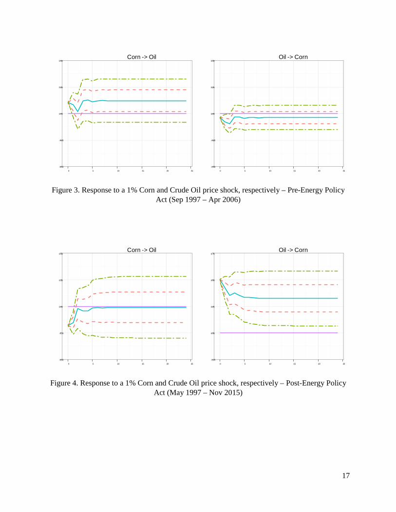
Cumulative impulse response functions calculated over the periods pre- and post-Energy

Policy Act are presented in figures 3 and 4, respectively. Each figure contains two plots

representing the percentage response of crude oil to a one percent shock to the price of corn, and

vice versa, during a 25-week period. The solid line represents the impulse response, and the inner

and outer dotted lines represent the 68% and 95% bootstrapped confidence intervals, respectively.

Comparing crude oil price responses between the two periods, we observe that before May 2006,

a shock to the price of corn had no statistically significant effect on the price of crude oil, except

on the week when the shock hit the crude oil market (figure 3). After May 2006, the price of crude

oil reacts slightly negatively to a one percent corn price shock. However, this effect is short-lived

and dies out one week after the shock (figure 4).

Focusing on corn price responses to shocks on the price of crude oil, it is evident that corn

prices became more responsive to crude oil price changes after the passage of the Energy Policy

Act. That is, before May 2006 corn price responses following shocks in the crude oil market are

close to zero and insignificant (figure 3). However, after May 2006, they become positive and

statistically significant (figure 4). Thus confirming that price dynamics between these two markets

have strengthened after the passage of the Act.

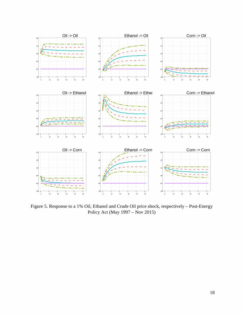
Finally, figure 5 shows the percentage responses of crude oil, ethanol and corn prices

following a one percent shock to each price series. On-diagonal plots represent cumulative

impulse responses of each price variable on itself. As expected, these responses are positive and

statistically significant in every case. Shocks to the price of oil impact both ethanol and corn

positively. However, this effect is more pronounced and persistent in the ethanol market. That is,

corn prices are affected by the oil price shock during a short period of time, which is not consistent

with our findings from model 2. A possible explanation for this finding relies on the reaction of

13

crude oil and corn prices to ethanol price shocks. Here, we observe that both price series show a

positive and statistically significant response. However, this response is larger in the corn market.

Consistent with previous literature, this result confirms that ethanol is an important link between

crude oil and corn markets. This is because once ethanol prices are introduced into the system,

corn price responses to crude oil shocks are substantially reduced. Moreover, corn price shocks

have no effect on oil and ethanol markets.

Conclusions

Causal and dynamic relationships between energy and agricultural markets have been a topic of

interest in the literature. This study supplements existing work by addressing the identification

problem encountered during the estimation of structural models which are typically used to explore

links between these markets. We use the method proposed by Rigobon (2003), which is based on

the heteroskedasticity of structural shocks. By identifying regimes of high volatility and low

volatility, we are able to estimate contemporaneous effects between variables without imposing

any additional or ad hoc restrictions in structural models. We implement this identifying method

because there is no strong a priori reason to support a specific set of contemporaneous exclusion

restrictions, and there is no reason to think that one exists, particularly in the study of agricultural

markets. This is a key component of this study since the reliability of the estimates reported, more

specifically in the analysis of the impulse responses, depends on the validity of the identifying

assumptions that have been imposed.

Using weekly average cash prices from September 1997 to November 2015, we estimate

two SVAR corresponding to the periods pre- and post-passage of the Energy Policy Act of 2005

to capture price dynamics between crude oil and corn prices. Then, we also estimate one SVEC

model that accounts for the cointegration relationship established when ethanol prices enter into

the system in the latter period. We find evidence of both unidirectional and bidirectional price

transmission between crude oil, ethanol and corn markets in the post-Act period. More

specifically, ethanol and corn prices positively react to a shock in the price of crude oil. Also,

crude oil prices have a positive response to ethanol price shocks, but fail to react following a corn

price shock. Corn prices are positively affected by ethanol price shocks indicating that the ethanol

market is the main link between energy and corn markets.

14

References

Bai, J. and P. Perron. (2003). “Computation and Analysis of Multiple Structural Change Models.” Journal of Applied Econometrics, 18: 1-22.

Baumeister, C. and L. Kilian. (2014). “Do Oil Prices Increases Cause Higher Food Prices?”

Economic Policy, 691–747. Ehrmann, M., M. Fratzscher and R. Rigobon (2011). “Stocks, Bonds, Money Markets and

Exchange Rates: Measuring International Financial Transmission.” Journal of Applied Econometrics, 26:948–974.

Godfrey, L. (2009). Bootstrap Tests for Regression Models. Basingstoke: Palgrave Macmillan. Goncalves, S. and L. Kilian. (2004). “Bootstrapping Autoregressions in the Presence of

Conditional Heteroskedasticity of Unknown Form.” Journal of Econometrics, 123:89-120. Kilian, L. (2013). “Structural Vector Autoregressions.” in: N. Hashimzade and M.A. Thornton

(eds.), Handbook of Research Methods and Applications in Empirical Macroeconomics, Cheltenham, UK: Edward Elgar, 2013, 515–554.

Kilian, L. and R. J. Vigfusson. (2011). “Are the Responses of the US economy Asymmetric in

Energy Price Increases and Decreases?” Quantitative Economics, 2: 419–453. Rigobon, R. (2003). “Identification through Heteroskedasticity.” The Review of Economics and Statistics, 85(4): 777–792. Serra, T. and D. Zilberman. (2013). “Biofuel-Related Price Transmission Literature: A Review.”

Energy Economics, 37: 141–151. Sims, C. A. (1980). “Macroeconomics and Reality.” Econometrica, 48: 1–48. Sims, C. A. (1986). “Are Forecasting Models Usable for Policy Analysis?” Federal Reserve Bank

of Minneapolis Quarterly Review, 10(1): 2–16.

15

Figure 1. Weekly Average Historical Price Volatilities for Crude Oil and Corn & Identified Regimes (Sep 1997 – Apr 2006)

1998 2000 2002 2004 2006

2040

6080

100

120

Crude Oil

1998 2000 2002 2004 2006

2040

6080

100

120

Corn

16

Figure 2. Weekly Average Historical Price Volatilities for Crude Oil and Corn & Identified Regimes (May 2006 – Nov 2015)

2008 2010 2012 2014 2016

2040

6080

100

120

140

Crude Oil

2008 2010 2012 2014 2016

2040

6080

100

120

140

Corn

17

Figure 3. Response to a 1% Corn and Crude Oil price shock, respectively – Pre-Energy Policy Act (Sep 1997 – Apr 2006)

Figure 4. Response to a 1% Corn and Crude Oil price shock, respectively – Post-Energy Policy Act (May 1997 – Nov 2015)

-0.50

-0.25

0.00

0.25

0.50

0 5 10 15 20 25

Corn -> Oil

-0.50

-0.25

0.00

0.25

0.50

0 5 10 15 20 25

Oil -> Corn

-0.50

-0.25

0.00

0.25

0.50

0 5 10 15 20 25

Corn -> Oil

-0.25

0.00

0.25

0.50

0.75

0 5 10 15 20 25

Oil -> Corn

18

Figure 5. Response to a 1% Oil, Ethanol and Crude Oil price shock, respectively – Post-Energy Policy Act (May 1997 – Nov 2015)

-0.5

0.0

0.5

1.0

1.5

2.0

0 10 20 30 40 50

Oil -> Oil

-0.5

0.0

0.5

1.0

1.5

2.0

0 10 20 30 40 50

Oil -> Ethanol

-0.5

0.0

0.5

1.0

1.5

2.0

0 10 20 30 40 50

Oil -> Corn

-0.5

0.0

0.5

1.0

1.5

2.0

0 10 20 30 40 50

Ethanol -> Oil

-0.5

0.0

0.5

1.0

1.5

2.0

0 10 20 30 40 50

Ethanol -> Ethanol

-0.5

0.0

0.5

1.0

1.5

2.0

0 10 20 30 40 50

Ethanol -> Corn

-0.5

0.0

0.5

1.0

1.5

2.0

0 10 20 30 40 50

Corn -> Oil

-0.5

0.0

0.5

1.0

1.5

2.0

0 10 20 30 40 50

Corn -> Ethanol

-0.5

0.0

0.5

1.0

1.5

2.0

0 10 20 30 40 50

Corn -> Corn

19

Table 1. Unit Root and Cointegration Tests Results for Weekly Average Oil, Corn and Ethanol cash prices

Test Test-statistics Sep 1997 – Apr 2006 May 2006 – Nov 2015 Augmented DF Constant Trend Constant Trend Oil -0.70 -1.98 -1.93 -2.99 Corn -2.60 -2.63 -1.99 -1.49 Ethanol -2.79 -2.83 Johansen Cointegration Max. Eigen. Trace Max. Eigen. Trace Model Oil–Corn r = 0 6.60 8.29 8.31 11.92 r ≤ 1 1.68 1.68 3.61 3.61 Model Oil–Ethanol–Corn r = 0 38.22** 50.44** r ≤ 1 9.24 12.22 r ≤ 2 2.98 2.98

Notes: AIC was used to determine appropriate lag lengths for the ADF test. The null hypothesis under the ADF test is nonstationary. The critical values are -2.87 and -3.42 for the 0.05 significance level, corresponding to the specifications using a constant (but not trend) and a trend, respectively. The null hypothesis under the Johansen cointegration test is the number of cointegration vectors (r). ** indicates rejection of the null hypothesis at the 0.05 significance level.

20

Table 2. Contemporaneous Parameter Estimates

Parameter Estimates Sep 1997 – Apr 2006 May 2006 – Nov 2015

Model Oil – Corn Coefficient p-value a Coefficient p-value a 𝛿𝛿1 0.103 0.001 -0.180 0.000 𝛿𝛿2 -0.036 0.083 0.504 0.000 𝑣𝑣𝑎𝑎𝐶𝐶(𝜀𝜀𝑂𝑂𝑂𝑂𝑂𝑂1 ) 22.109 0.000 40.834 0.000 𝑣𝑣𝑎𝑎𝐶𝐶(𝜀𝜀𝐶𝐶𝐶𝐶𝐶𝐶𝐶𝐶1 ) 7.345 0.000 23.756 0.000 𝑣𝑣𝑎𝑎𝐶𝐶(𝜀𝜀𝑂𝑂𝑂𝑂𝑂𝑂2 ) 17.344 0.000 10.705 0.000 𝑣𝑣𝑎𝑎𝐶𝐶(𝜀𝜀𝐶𝐶𝐶𝐶𝐶𝐶𝐶𝐶2 ) 13.157 0.000 16.153 0.000 p-value b p-value b 𝑣𝑣𝑎𝑎𝐶𝐶(𝜀𝜀𝑂𝑂𝑂𝑂𝑂𝑂1 )/𝑣𝑣𝑎𝑎𝐶𝐶(𝜀𝜀𝑂𝑂𝑂𝑂𝑂𝑂2 ) 1.274 0.000 3.814 0.000 𝑣𝑣𝑎𝑎𝐶𝐶(𝜀𝜀𝐶𝐶𝐶𝐶𝐶𝐶𝐶𝐶1 )/𝑣𝑣𝑎𝑎𝐶𝐶(𝜀𝜀𝐶𝐶𝐶𝐶𝐶𝐶𝐶𝐶2 ) 0.558 1.000 1.471 0.000 Model Oil–Ethanol–Corn p-value a 𝛿𝛿12 -0.062 0.003 𝛿𝛿13 -0.139 0.000 𝛿𝛿21 0.056 0.002 𝛿𝛿23 -0.095 0.071 𝛿𝛿31 0.435 0.000 𝛿𝛿32 0.199 0.000 𝑣𝑣𝑎𝑎𝐶𝐶(𝜀𝜀𝑂𝑂𝑂𝑂𝑂𝑂1 ) 40.616 0.000 𝑣𝑣𝑎𝑎𝐶𝐶(𝜀𝜀𝐸𝐸𝑡𝑡ℎ𝑎𝑎1 ) 7.625 0.000 𝑣𝑣𝑎𝑎𝐶𝐶(𝜀𝜀𝐶𝐶𝐶𝐶𝐶𝐶𝐶𝐶1 ) 23.368 0.000 𝑣𝑣𝑎𝑎𝐶𝐶(𝜀𝜀𝑂𝑂𝑂𝑂𝑂𝑂2 ) 10.818 0.000 𝑣𝑣𝑎𝑎𝐶𝐶(𝜀𝜀𝐸𝐸𝑡𝑡ℎ𝑎𝑎2 ) 12.712 0.000 𝑣𝑣𝑎𝑎𝐶𝐶(𝜀𝜀𝐶𝐶𝐶𝐶𝐶𝐶𝐶𝐶2 ) 15.753 0.000 p-value b 𝑣𝑣𝑎𝑎𝐶𝐶(𝜀𝜀𝑂𝑂𝑂𝑂𝑂𝑂1 )/𝑣𝑣𝑎𝑎𝐶𝐶(𝜀𝜀𝑂𝑂𝑂𝑂𝑂𝑂2 ) 3.754 0.000 𝑣𝑣𝑎𝑎𝐶𝐶(𝜀𝜀𝐸𝐸𝑡𝑡ℎ𝑎𝑎1 )/𝑣𝑣𝑎𝑎𝐶𝐶(𝜀𝜀𝐸𝐸𝑡𝑡ℎ𝑎𝑎2 ) 0.599 1.000 𝑣𝑣𝑎𝑎𝐶𝐶(𝜀𝜀𝐶𝐶𝐶𝐶𝐶𝐶𝐶𝐶1 )/𝑣𝑣𝑎𝑎𝐶𝐶(𝜀𝜀𝐶𝐶𝐶𝐶𝐶𝐶𝐶𝐶2 ) 1.483 0.000

Notes: p-value (a) corresponds to the test of the null hypothesis 𝐻𝐻0: 𝛿𝛿𝑗𝑗 = 0. p-value (b) corresponds to the test of the null hypothesis 𝐻𝐻0: 𝑣𝑣𝑎𝑎𝐶𝐶(𝜀𝜀𝑔𝑔1)/𝑣𝑣𝑎𝑎𝐶𝐶(𝜀𝜀𝑔𝑔2) ≤ 1, for market 𝑔𝑔.