Embed Size (px)
Citation preview
Identification And Simulation Of An Automated Guided
Vehicle For Minimal Sensor Applications
A thesis presented for the degree of
Master of Engineering in Mechanical Engineering
in the University of Canterbury,
Christchurch, New Zealand.
By
Aaron Dann B.E (Mech) (Hans.)
1996
ABSTRACT
The problem of controlling an Automated Guided Vehicles (AGV) with the minimum
number of sensors is considered. Sensors add cost and complexity to an AGV both
electrically and in terms of increased computational requirements of the controller.
Computer simulations are proposed to model the behaviour of the AGV Models of
the dynamics of an AGV are proposed and simulated at varying levels of complexity
using commercially available numerical software.
In order to model the AGV accurately, aspects of the control system and the physical
system had to be analysed. Laboratory experiments were designed and performed, and
the results were analysed to determine the dynamic properties of sub-systems of the
AGV
To provide a datum for comparison to the simulations, measurements were made of
the performance of an AGV under a variety of control conditions corresponding to the
computer models. Comparisons of the simulations and the AGV performance are
discussed and suggestions are made for improving the AGV and its control system.
The models presented in this thesis demonstrate a good correlation for low
performance AGV s in non-rigorous conditions, or well loaded AGV s on good traction
surfaces. However they do not accurately represent the AGV at the limits of traction.
Two mechanical improvements to the University of Canterbury (UOC) Mle-II AGV
are suggested, including the addition of softer compound tyres for use on hard, painted
surfaces, and the design of a gear train with lower backlash.
1
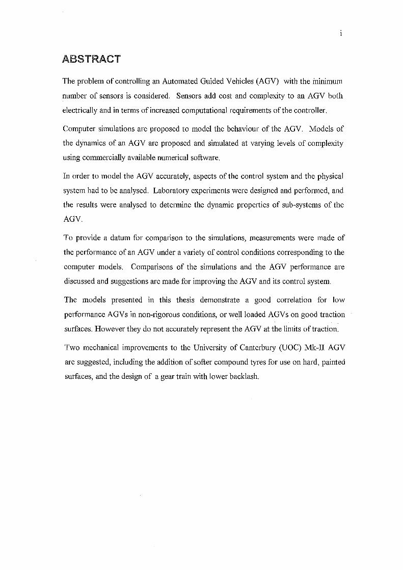
TABLE OF CONTENTS
1. fflTRODUCTION ............................................................................................. " ... " ...................... 1
1.1 ADVANTAGES OF AGVs OVERMANuALLABOUR ....................................................................... 2
1.2 OPERATION ENVIRONMENT CONSIDERATIONS: ........................................................................... 2
1.3 AGVMECHANICALSYSTEM ..................................................................................................... 4
1.4 AGV ELECTRICAL SySTEMS ...................................................................................................... 5
1.5 THE COMPLE}'1TY OF THE AGV SySTEM .................................................................................... 6
1.6 ISSUES OF REVERSING ................................................................................................................ 7
1. 7 SAFETY CONCERNS ................................................................................................................. 10
2. AGV SYSTEM DyNAMICS ...................................................................................................... 12
2.1 INTRODUCTION To COMPUTER SllvIULATION ............................................................................. 12
2.2 DERIVATION OF THE AGV MODEL .......................................................................................... 15
2.2.1 Notation ......... ................................................................................................................ 15
2.2.2 Introduction .... ................................................................................................................ 16
2.2.3 The AGT,ns Equations OfA1.otion ..................................................................................... 17
2.2.4 AGV Sub~systems ................................................................................. ........................... 17
2.2.5lvfodel Developnlent ................................................ ~ ......................................................... 19
2.3 DETERIvIINING SYSTEM PROPERTIES USING SYSTEM IDENTIFICATION METHODS ........................ 21
2.4 THEEXPERIMENTS: ................................................................................................................. 22
2.4.1 Recording the dynamics of the DCMC and gear train ..................................................... 22
2.4.2 Recording and analysis of the Electric A1.otors and drive train ....................................... 23
2.4.3 Recording the performance of the A GV under closed loop controL ............................... 24
2.5 IMPLEMENTATIONOFTHEAGV MODEL .................................................................................. 27
2.5.1 Non-Linear - Second Order Model .. ............................................................................... 28
2.5.2 Complete Simple non~Unear model ................................................................................. 30
2.5.3 Complete Complex Model- second order AGV + backlash ............................................. 31
3, AGV ELECTRICAL SYSTEMS ....................................... , ....................................................... 34
3.1 AGV ELECTRICAL SYSTEMS .................................................................................................... 34
3.1.1 AGV 80C552lvficrocontroller Board .............................................................................. 34
11
3.1.2 Dynamic Controls Motor Controller (DCMC) ................................................................ 35
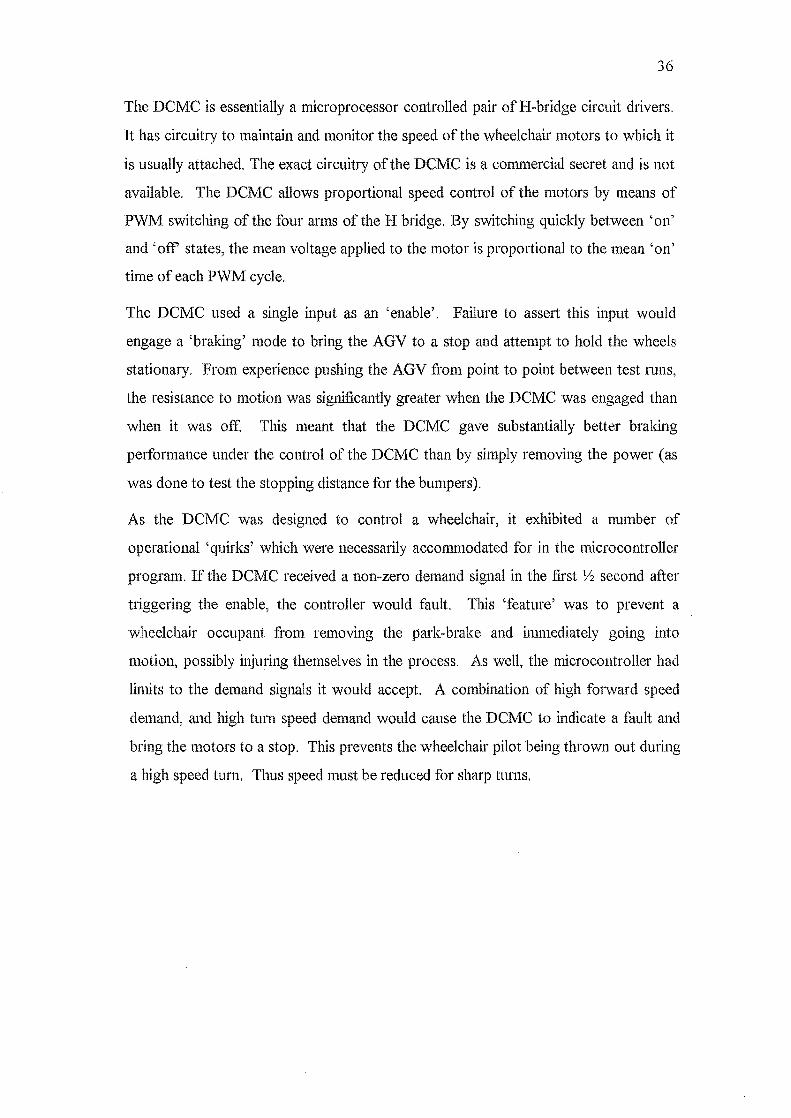
3.1.3 Guide Wire Proximity Circuits ........................................................................................ 37
3.2 AGV SUPPORTELECTRONICS .................................................................................................. 38
3.2.1 Guide vVire Signal Generator ......................................................................................... 39
3.2.2 Host PC .......................................................................................................................... 40
4. AGV PROJECT SOFTW ARE ..................... t1, ••••••••••• t ••• '1 •• t ••• J ••••• , •• , ••• , ••• , •••••• , •••••••••••• ,., ••• " ••••••••• .::tl
4.1 MICROCONTROLLER PROGRA1vlMING SOFrW ARE ....................................................................... 41
4.2 HOST PC SUPPORT SOFTWARE ................................................................................................. 42
4.3 AGV MIcRocONTROLLER SOFrWARE ..................................................................................... 44
4.3.1 Embedded Controller Soflware .............................................................................. ......... 44
4.3.2 Utility and User Interface Software ................................................................................ 45
4.3.3 The P-D Controller PLAYTIA;fE.C .................................................................................. 47
5. RESULTS OF SYSTEM IDENTIFICATION EXPERIMENTS: ............................................. 49
5.1 ANALYSING THE ELECTRIC MOTORS AND DRIVE TrWN RECORDING ........................................ 49
5.2 SYSTEM IDENTIFICATION ANALYSIS OF THE DCMC CONTROLLING A DC MOTOR ........... " ....... 50
5.2.1 Case 1-1 Modelling the DCMC as a simple gain . ............ "" ...... " .................................... 52
5.2.2 Case 2-1 Modelling the DCMC as a simple feedback controller ............. " ..................... " 54
5.2.3 Case 2-11 Modelling the DClvfC as a P-Ifeedback controller .. " ........ , ......... , .. ,'" ............. 57
5.2.4 Discussion of the system identijicatiol1lllodels ............................ " ...... " .......................... 59
6. RESULTS AND COMPARISONS OF SIMULATIONS AND LABORATORY TESTS ........ 63
6.1 INlTlAL CONDITIONS FOR AGV LABORATORY TESTING ............................................................ 63
6.2 RESULTS OF SllvlULATIONS ........................................................................... " ......................... 63
6.2.1 Simple Linear Second Order Nfodel ................................................................................ 63
6.2.2 COl1lplete IVon-Linear Nfodel ......................................... " ......... " ............... " ................... 64
6.2.3 Complete Complex Second Order model with Backlash .................................................. 65
6.3 COMPARISON OF LAB RESULTS Ai'lD SIlYlULATIONS .................................................................... 65
6.3.1 Comparison of the Backlash Nfodelwith the Experimental results .................................. 65
6.3.2 Potential Sources of Model Inaccuracy ................................................ " ........................ 66
6.3.3 Potential Sources of Experimental Error ........................................................................ 66
iii
7. CONCLUSIONS ......................................................................................................................... 78
8 .. REFERENCES .......................................................................................... , .................................. 80
APPENDIX A: AGV MICRO CONTROLLER 'C' CODE ........................................................... 82
AGVAD.C ................................................................................................................................... 82
AGVCONT.C .......................... , .................................................. ,.,.' .... , .......... ,.,., ........ , ............... 82
AGVDRIVE.C ............................................................................................................................. 84
AGVINT.C ............................................................................................................................. , ... ,85
AGVLOOP.C .............................................................................................................................. 85
AGVPOS.C ................................................................................................................................. 86
AGVSER.C ................................................................................................................................. 88
PLAYTIME.C ............................................................................................................................. 90
AGVVARS.C .............................................................................................................................. 93
APPENDIX B: SUPPORT PC 'e' CODE ..................................................................................... 95
IDSYS.C DATA LOGGING UTILITY ................................................................................................. 95
APPENDIX C: GRAPHS OF THE SYSTEM IDENTIFICATION TESTS ............................... 100
IV
TABLE OF FIGURES
FIG. 1.1- AGV VIEWED FROM UNDERSIDE, NOTE THE BATTERY COMPARTMENTS, GUIDE WIRE ANTENNAE,
AND CASTORS ............................................................................................................................. 4
FIG 1.1- SIDE VIEW OF AGV MOUNTING AN INCLINED RAMP .................................................................. 4
FIG 1.2, VARIOUS GUIDE WIRE SENSOR ARRANGEMENTS FOR THE AGV ................................................ 9
FlG. 1.3-AGV BUMPERS AND MICROSWITCHES ................................................................................... 10
FIG. 2.4- ENERGY FLOW IN A SIMPLIFIED BOND GRAPH OF THE AGV .................................................... 17
FIG. 2.5 - DC MOTOR, ELECTRICAL CIRCUIT AND SIMPLIFIED BOND GRAPH ........................................ 18
FIG. 2.6- DC MOTORSIMULINKBLOCKDIAGRAM .............................................................................. 18
FIG. 2.7 REDUCTION GEAR TRAIN, MECHANICAL REPRESENTATION ANDBLOCKDIAGRAlvI.. ................ 19
FlG. 2.8- COMPLETE AGV BLOCK DIAGRAM ...................................................................................... 20
FIG. 2.9- BACKEMF, DC MOTOR ROTOR INERTIA TEST RIG ................................................................ 24
FIG. 2.10- AGVPATHMAIUaNGPEN .................................................................................................. 26
FIG. 2.11- TYPICAL SIMULINK SCREEN-SHOT ...................................................................................... 27
FIG. 2.12- SUvIULINKSATURATIONBLOCK, ±23.5VDC ........................................................................ 28
FIG. 2.13 - SIMULINKSCREEN: SUvIPLENON-LINEAI~AGVMoDEL ..................................................... 29
FIG. 2.14- SIMULINK SCREEN: POSITION CALCULATION BLOCK ............................................................. 29
FIG. 2.15- GUIDE WIRE SENSOR, SENSOR STRENGTH DIAGRAM ............................................................ 30
FIG. 2.16 - SUvIULINK SCREEN: COMPLETE SIMPLE NON-LINEAI~ MODEL ............................................. 31
FIG. 2.17 - SIMULINK SCREEN: AGV KINEMATICS COMPLETE WITH BACKLASH ..................................... 32
FIG. 2.18- DIAGRAM OF THE GEAI~BACKLASHMODEL. ....................................................................... 32
FIG. 2. 19-5UvIULINK BLOCK DIAGRAM OF THE GEAR TRAIN BACKLASH MODEL. ................................... 33
FIG. 2.20 - COMPLETE80c552 MICRO CONTROLLER BLOCK INCLUDING; THE LOW PASS (-3DB @100Hz)
FILTERS ON THE PWM, TIMING DELAYS AND QUANTfSATION OF THE SENSOR SIGNAL ................... 33
FIG. 3.1 THE MICRO CONTROLLER CONTROL SUB-SYSTEMS ................................................................ 34
FIG. 3.2 (A) PWM DUTY CYCLE (B) H-BRIDGE SCHEMATIC ................................................................ 35
FIG. 3.3- MECHANICAL LAYOUT OF THE GUIDE WIRE SENSORS ............................................................ 37
FIG. 3.4- GUIDE WIRE SENSING CIRCUIT ............................................................................................ 37
FIG. 3.5 - GUIDEWlRESENSORSIGNALPLOT ...................................................................................... 38
v
FIG. 3.6- PHOTO, THEEXPERIMENTALRIG ......................................................................................... 39
FIG. 4.1- BLOCK DIAGRAM, SOFTWARE FUNCTIONS IN IDSYS. C ........................................................ 43
FIG. 4.2 - DIAGRAM OF AGV CONTROL SOFTW ARE INTERFACE ......................................................... .44
FIG. 4.3- GUIDE WIRE CIRCUIT FOR THEAGV RUNNINGPLAYTIME.C ............................................ .47
FIG. 5.1- RESULTS OF THE FALLING WEIGHT TEST .............................................................................. 50
FIG. 5.2- BLOCK DIAGRAM OF CASE (I) DCMC MODEL CANDIDATE ..................................................... 52
FIG. 5.3- BLOCK DIAGRAM OF CASE 2-1 DCMC MODEL CANDIDATE, SIMPLE FEEDBACK CONTROLLER .. 55
FIG. 5.4- BLOCK DIAGRAM OF CASE 2-II DCMC MODEL CANDIDATE, PI FEEDBACK CONTROLLER ........ 57
FIG. 5.5 Rw21.DAT, TRYSS2.M, DCMC MODEL2-I.. ........................................................................ 61
FIG. 5.6 Rw21.DAT WITH: TRYSS3.M, DCMC MODEL2-II ................................................................ 62
FIG. 6.1- AGV LINEAR MODEL PATH AT VARYING PROPORTIONAL GAIN .............................................. 68
FIG. 6.2- AGVLINEARMoDELPATHS WITH VARYING PROPORTIONAL GAIN ......................................... 69
FIG. 6.3- COMPLETE NON-LINEAR MODEL PATHS WITH VARYING PROPORTIONAL GAIN (0.1 - 1.0) ......... 70
FIG. 6.4- COMPLETE NON-LINEAR MODEL PATHS WITH VARYING PROPORTIONAL GAIN (1.5-4.0) ........... 71
FIG. 6.5- AGV NON-LINEAR BACKLASH MODEL PATHS WITH VARYING PROPORTIONAL GAIN (2.0-6.0) ... 72
FIG. 6.6- AGV PAPER TRACE, RUN#l ................................................................................................ 73
FIG. 6.7- AGV PAPER TRACE, RUN #2 ................................................................................................ 74
FIG. 6.8- AGV PAPER TRACE, RUN #3 ................................................................................................ 75
FIG. 6.9- COMPARISON OF THE EXPERIMENTAL RESULTS TO THE AGV BACKLASH MODEL ..................... 76
FIG. 6.10- COMPARISON OF THE EXPERIMENTAL RESULTS TO THE AGV NON-LINEAR MODEL ............... 77

vi
Acknowledgments
I am indebted to my supervisor Dr G.R Dunlop for his aid and encouragement during
the course of this work.
I would like to thank the Applied Mechanics Laboratory Technician (and now PhD
candidate) Andy Cree for his valuable aid in all things electrical and mechanical, and
the Electrical and Computer Workshop Technician Julian Murphy for his help with
things electronic.
I also wish to thank my fellow postgraduate students without whom the longest days
would have seemed much longer.
I especially wish to thanlc my fiance Stephanie for her unbounded patience and support
during the course of this work.
AGV
AID
ADC
AJ.\1N
DC
DCMC
DSP
EMF
EPROM
FET
FM
IC
IDE
I/O
LCD
]\.IICU
NZ
PC
PSK
PWM
UOC
UPP
Automated Guided Vehicle
Analog to Digital
Analog to Digital converter
Artll1cialNeuralNetvvork
Direct Current Motor
DC motor controller
Digital Signal Processor
Electro-motive force
Electrically Programmable Read Only Memory
Field Effect Transistor
Frequency Modulation
Integrated Circuit
Integrated Development Environment
Input/Output
Liquid Crystal Display
Microcontroller Unit
New Zealand
Personal Computer
Phase Shift Keying
Pulse Width Modulation
University of Canterbury
Universal Pulse Processor
vii
1
1. INTRODUCTION
The conventional pedestrian electric pallet truck is able to reverse under a load, lift it
and then drive away following the walking operator. The development of accurate
methods for controlling these vehicles has allowed the introduction of automated
versions of these load carrying trucks. These automated versions are known as
Automated Guided Velncles or AGV s.
The University of Canterbury AGV MK II is an autonomous guided vehicle
characterised by it's steering and driving axis geometry. The AGV achieves its steering
by actuating the drive wheels at the different speeds, in much the same way as tracked
vehicles.
This thesis presents the results of modelling the UOC AGV MK II in forward motion,
with attention to options for driving the AGV in reverse. Mathematical models were
developed to describe the dynamics of the AGV. These models were simulated using
The MathWorks 'MATLAB' software package along with the SIMULINK simulation
tools.
To ensure the accuracy of the AGV the simulation models, experiments were designed
to determine the properties (co-efficients, m~ments of inertia etc .. )of the AGV's sub
systems. The results from these experiments were analysed using the MATLAB and
the System Identification Toolbox.
To validate the models the actual performance of the AGV needed to be compared to
the results from the simulations. To ascertain this the UOC AGV MK II was equipped
with a micro controller based control system, sensors and electronic motor drive unit,
and programmed to operate under the control methods used in the simulations. The
AGV path was tracked and recorded . Finally the performance of the simulation was
compared with the measured performance of the AGV.
2
1.1 ADVANTAGES OF AGVs OVER MANUAL LABOUR.
There are a number of important benefits to be gained from the use of AGV, systems.
Quite apart from the labour savings, these are mostly concerned with the transport
properties:
(i) smooth regular acceleration and deceleration: Prevents product damage because
the payload is not subject to the unnecessary stress of uncontrolled acceleration.
Also the components of the AGV will have a greater lifetime as the stresses are
known and controllable, and are not likely to exceed the rated design loads. This
cannot always be said for manually driven fork lift trucks.
(ii) predictable (See (i) above) and controllable path, always travels by the shortest
route: Although AGVs are not necessarily the fastest material handling method,
they are the most flexible. They allow the product to be moved to the destination
by the shortest available route at all times. However, this is subject to the
effectiveness of the traffic management system.
(iii) regular service: The AGV does not make stops for the lunch, tea breaks etc ...
(iv) minimal support services: The AGV does not require the creature comforts of
human workers, heating, lighting, hygiene, facilities, superannuation etc ...
1.2 OPERA TlON ENVIRONMENT CONSIDERA TlONS:
AGV s will repetitively follow the allocated guide path, and because their wheels are
generally hard on the work surface. The preferred sUlface is hard concrete since they
will quickly wear tracks in soft surfaces such as carpet, vinyl or asphalt (tar).
In the case of wire guided AGV's, steel sheets or steel reinforcing mesh, on or near the
surface can alter the signal from the guide wire. Appropriately spaced steel rods can
however, be used as a path identification bar code.
Communication of AGV s with a central warehouse computer can be maintained by
several methods:
(i) Radio Modem
(ii) Inductive Loop buried at decision intervals
(iii) Inductive wire buried alongside the guidance wire.
(iv) Physical connection data points
(v) FM or PSK (phase Shift Keying) applied to the guidance wire.
3
The first method can suffer from the problems of multiple paths le. interference
patterns, if the systems are not properly set up. The radio signal can be reflected from
multiple surfaces and in the high MHz frequency range, the wavelength «1m) can give
rise to antinodes in the work space where the radio signals suffer destlUctive
interference thus leaving the AGV without any communication with the base
computer. Fisher and Paykel NZ use AGV s in their refrigerator manufacturing plant
as an integral feature of their flexible manufacturing system. These AGV s use radio
modems to communicate with central routing computers and programmable
controllers.
The second method has been used in a number of installations [13], however if the
AGV stops away from the decision loop, it has no way to communicate with the
central computer, and must simply wait until it is discovered. The third method is the
most common, because the AGV follows the guidance wire and the adjacent induction
wire gives immediate feedback to the central computer. A packet switching TDM can
be incorporated when several AGV's are communicating on the same induction wire.
Also, two signal pick-ups are required since the inductive wire position depends on
which way the AGV is going. The fourth method is obvious but suffers from the
same problems as method (ii).
The method (v) is proposed for the UOC (University Of Canterbury) AGY. The
induction wire and the guidance wire are the same, which further reduces the capital
investment and installation costs. In addition since the guidance pick-up is used for the
communications signal as well, the two signal pick-ups required for (iii) are eliminated.
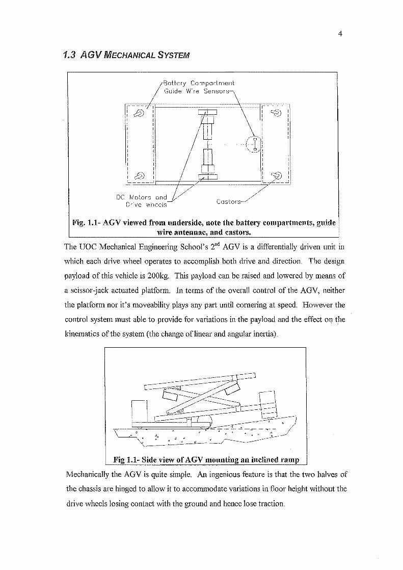
1.3 AGV MECHANICAL SYSTEM
Battery Compartment Guide Wire Sensors
DC Motors and Drive wheels Castors
Fig. 1.1- AGV viewed from underside, note the battery compartments, guide wire antennae, and castors.
4
The UOC Mechanical Engineering School's 2nd AGV is a differentially driven unit in
which each drive wheel operates to accomplish both drive and direction. The design
payload of this vehicle is 200kg. This payload can be raised and lowered by means of
a scissor..jack actuated platform. In terms of the overall control of the AGV, neither
the platform nor it's moveability plays any part until cornering at speed. However the
control system must able to provide for variations in the payload and the effect on the
kinematics of the system (the change of linear and angular inel1ia).
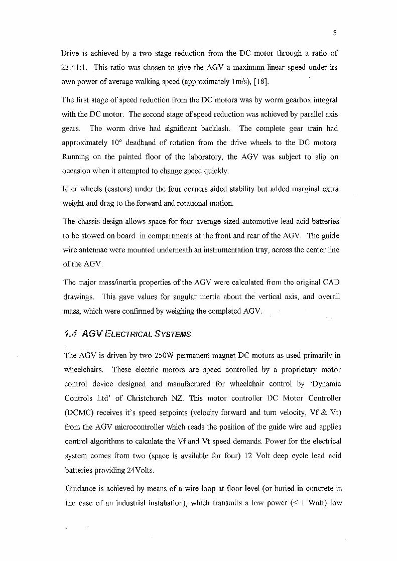
Fig 1.1- Side view of AGV mounting an inclined ramp
Mechanically theAGV is quite simple. An ingenious feature is that the two halves of
the chassis are hinged to allow it to accommodate variations in floor height without the
drive wheels losing contact with the ground and hence lose traction.
5
Drive is achieved by a two stage reduction from the DC motor through a ratio of
23.41: 1. This ratio was chosen to give the AGV a maximum linear speed under its
own power of average walking speed (approximately hn/s), [18].
The first stage of speed reduction £i'om the DC motors was by worm gearbox integral
with the DC motor. The second stage of speed reduction was achieved by parallel axis
gears. The worm drive had significant bacldash. The complete gear train had
approximately 10° deadband of rotation from the drive wheels to the DC motors.
RUlU1ing on the painted floor of the laboratory, the AGV was subject to slip on
occasion when it attempted to change speed quicldy.
Idler wheels (castors) under the four corners aided stability but added marginal extra
weight and drag to the forward and rotational motion.
The chassis design allows space for four average sized automotive lead acid batteries
to be stowed on board in compartments at the front and rear of the AGY. The guide
wire antennae were mounted underneath an instrumentation tray, across the center line
of the AGY.
The major mass/inertia properties of the AGV were calculated from the original CAD
drawings. This gave values for angular inertia about the vertical axis, and overall
mass, which were confirmed by weighing the completed AGY.
1.4 AGV ELECTRICAL SYSTEMS
The AGV is driven by two 250W permanent magnet DC motors as used primarily in
wheelchairs. These electric motors are speed controlled by a proprietary motor
control device designed and manufactured for wheelchair control by 'Dynamic
Controls Ltd' of Christchurch NZ. This motor controller DC Motor Controller
(DCMC) receives it's speed setpoints (velocity forward and turn velocity, Vf & Vt)
from the AGV microcontroller which reads the position of the guide wire and applies
control algorithms to calculate the Vf and Vt speed demands. Power for the electrical
system comes from two (space is available for four) 12 Volt deep cycle lead acid
batteries providing 24 Volts.
Guidance is achieved by means of a wire loop at floor level (or buried in concrete in
the case of an industrial installation), which transmits a low power « 1 Watt) low
6
fi"equency « 1 00 KHz) signaL Two tuned receivers attached to the underside of the
AGV act as antennas. The AGV seeks to place the sensors either side of the guide
wire. The differential signal from the sensors is used to determine the AGV centre line
location with respect to the guide wire. The AGV's controller is an 8-bit embedded
80C552 microcontroller (a derivative of the Intel MCSS1 family c.£. [24],[25]) with
the on board facility for analog signal measurement and pulse timing generation and
measurement. The microcontroller is coupled with an array of push buttons and an
LCD panel for a user interface.
For progranuning testing and data collection, the AGV microcontroller connects to an
IBM PC mnning DOS and a commercial 'C' programming suite for the 8051 family of
microcontrollers. This enables the microcontroller to be programmed quickly using
ANSI-C.
The System Identification input and output variables were obtained using a
multipurpose I/O card containing analog inputs plus digital inputs and outputs
(Universal Pulse Processor or UPP card designed and built by the Mechanical
Engineering Department) which was installed in the host Pc. This card measured
timing pulses from the rotary encoders as well as the back El'VIF voltages for the
AGV's electric motors. It also measured the demand voltages to the DCMC.
1.5 THE COMPLEXITY OF THE AGV SYSTEM
Minimising the number of sensors on an AGV should produce a cheaper and more
robust product. Ultimately the control system could be reduced to an analog wire
guidance section supervised by a digital micro controller for path planning and routing
control. However the relatively low cost of micro controllers with analog input
channels, makes that simplification unnecessary. Also micro controllers are generally
more flexible than analog circuitry and the development of different control strategies
is considerably easier.
In the case of the UOC AGV, there are eight analog input channels on the
microcontroller, and the AGV uses nearly all these in its current configuration:
-2 Analog inputs for guide wire sensors
02 Analog inputs for manual control joystick
7
EIl1 Analog input for battery voltage level
Ii) 1 Analog input for ultra-sonic distance measurement (if using a commercial
integrated unit, otherwise it would be possible to achieve the same results with a
digital output to trigger a transmitter, and a timer input to measure the echo).
An increase in the number of sensors is not a problem to the AGV micro controller
until the total number of sensors becomes greater that the number of available. In the
case of the UOC AGV 11K II, there are still two channels available. To use a number
of sensors greater than those immediately available would require additional circuitry
to read the signals, either multiplexing analog chips to select from the analog sensor
signals, or additional analog to digital conversion chips (possibly memory mapped into
the microcontroller).
Eight channel analog multiplexing chips cost from NZ$6 to $25 (single chip sales
March '96), with 12 bit analog to digital conversion ICs costing from NZ$48 to $100
and above. There are a number of peripheral AID converters on the market, including
the Analog Devices, single chip serial AID. These chips provide multiple channels of
analog to digital conversion, the results of which can be accessed by the
micro controller via a serial protocol, these currently sell for around $25 in single units.
The advantage of the serial chips is that they require little additional circuitry and often
more chips can be networked to the micro controller without difficulty.
When the price of additional analog inputs is compared to the pnce of the
micro controller, 80c552 (NZ$38), the cost of the micro controller board is increased
markedly with additional analog input channels above the existing eight.
1.6 ISSUES OF REVERSING
In AGV installations the necessity to reverse the AGV is most often limited to
reversing out of docking stations where the distance to travel is shOlt, and the well
within the range of dead reckoning ,Imai et a1.[13]. In the case where the AGV has
only two guide wire sensors, its ability to reverse is limited as the AGV represents an
unstable system with bounded ability to correct for disturbances.
Guide Wire Path
(; ifl C Q) (j)
8
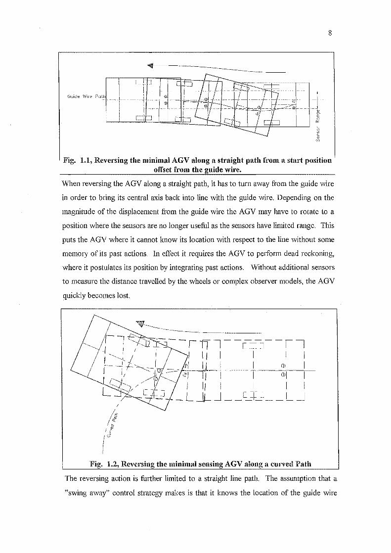
Fig. 1.1, Revel'sing the minimal AGV along a straight path from a start position offset from the guide wire.
When reversing the AGV along a straight path, it has to turn away from the guide wire
in order to bring its central axis back into line with the guide wire. Depending on the
magnitude of the displacement fi'om the guide wire the AGV may have to rotate to a
position where the sensors are no longer useful as the sensors have limited range. TIus
puts the AGV where it cannot Imow its location with respect to the line without some
memory of its past actions. In effect it requires the AGV to perform dead reckoning,
where it postulates its position by integrating past actions. Without additional sensors
to measure the distance travelled by the wheels or complex observer models, the AGV
quickly becomes lost.
(
"I I
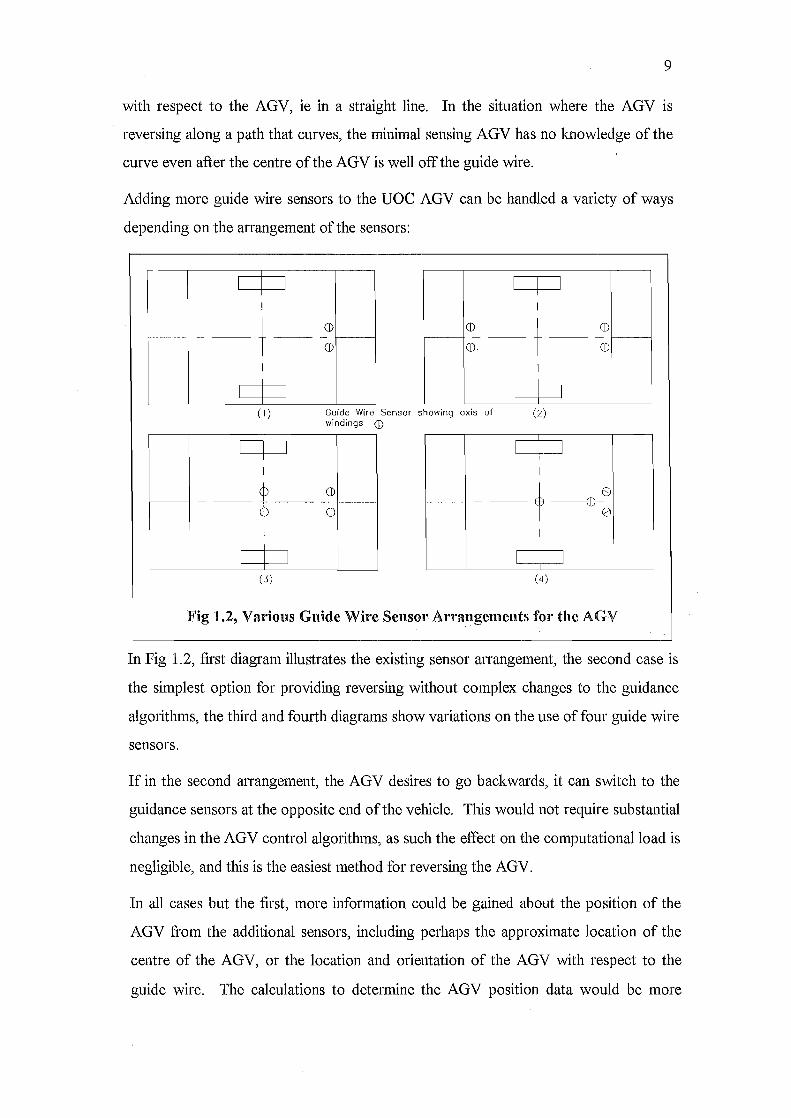
Fig. 1.2, Reversing the minimal sensing AGV along a curved Path
The reversing action is further limited to a straight line path. The assumption that a
"swing away" control strategy malces is that it knows the location of the guide wire
9
with respect to the AGV, ie in a straight line. In the situation where the AGV is
reversing along a path that curves, the minimal sensing AGV has no knowledge of the
curve even after the centre of the AGV is well off the guide wire.
Adding more guide wire sensors to the DOC AGV can be handled a variety of ways
depending on the arrangement of the sensors:
I I I I I I
I I
--t--~ m t m --- ---
(j) m I I I I
I I I I I I
(1) Guide Wire Sensor showing axis of windings m (2)
I I I I I I I I
I I
--*--~ --- f --4D-~ I I
I
l 1 I I I I
(3) (4)
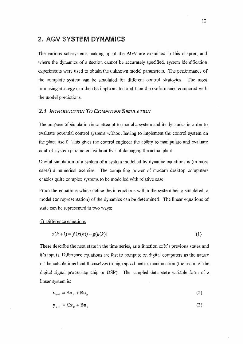
Fig 1.2, Various Guide Wire Sensor Arrangements for the AGV
In Fig 1.2, first diagram illustrates the existing sensor alTangement, the second case is
the simplest option for providing reversing without complex changes to the guidance
algorithms, the third and fourth diagrams show variations on the use of four guide wire
sensors.
If in the second arrangement, the AGV desires to go backwards, it can switch to the
guidance sensors at the opposite end of the vehicle. This would not require substantial
changes in the AGV control algorithms, as such the effect on the computational load is
negligible, and this is the easiest method for reversing the AGV.
In all cases but the first, more information could be gained about the position of the
AGV from the additional sensors, including perhaps the approximate location of the
centre of the AGV, or the location and orientation of the AGV with respect to the
guide wire. The calculations to determine the AGV position data would be more

10
complex, as there are a greater number of variables to manipulate. The additional load
on the microcontroller due to the extra variables would be dependant on the exact
algorithm, but could be expected to increase the load by a factor of two to four by
reason that each of the variables would have a third (and possible fourth) variable to
interact with.
The strength of the sensor signal varies with the angle that the sensor makes with the
guide wire such that when the sensor's axis is parallel to the guide wire the signal is
zero. In the fOUlih illustration, the arrangement of the three sensors has an additional
advantage over the arrays of pairs in the other illustrations, at least one of the sensors
will always be able to detect the guide wire. This has the advantage that the AGV
would be able to approach the guide wire from a more oblique angle without losing the
signal, although intuitively, the algorithm to determine the AGV position and
orientation would be quite complicated.
In short, to reverse the AGV under the minimal sensor criteria is difficult without
additional sensors or control strategies. The most simple way around the problem of
reversing the AGV is not to reverse it at all, but to add a second pair of sensors at the
opposite end of the AGV and use them to drive the AGV forward in the opposite
direction. The simulations in this thesis deal with developing a model of the UOC
AGV 11K II for the case of driving the AGV forward.
1.7 SAFETY CONCERNS
FOAM RUBBER BUMPER
Fig. 1.3-AGV bumpers and micl'oswitches
Front and rear bumpers were attached to the AGV to prevent damage to persons and
the AGV alike. These bumpers were made of soft foam rubber bent around the front of

11
the AGV in such a fashion as to trigger the stop program on the microcontroller at the
slightest touch of an obstacle.
The bumpers were designed to be fail-safe. The braid connecting the bumper and the
microswitch was in tension and if it slackened for any reason, the microswitch would
open with the loss of tension. The electrical circuit detecting the bumper was short
circuit or 'normally closed' so any loss of power or a faulty comlection would open the
circuit and the micro controller would cause the AGV to stop.
The distance the AGV travels from touching an obstacle to coming to a complete halt
from loss of drive power was less than the depth of the bumpers. In this way the AGV
would come to rest before exerting any substantial force on the obstacle. Stopping was
achieved by removing the 'run' signal from the DCMC, which would engage a
'braldng' mode to bring the AGV to a stop and attempt to hold the wheels stationary.
This braked the AGV in a substantially shorter stopping distance than simply removing
the power from the DC motors and leaving the AGV to coast to a stop.
NOTE:' A peculiarity of the stop circuit was discovered during lab trials. If the bumper
was depressed when the micro controller was reset, the bumper would not trigger a
stop during any subsequent collisions. This 'feature' of the micro controller was related
to the reset state of the external interrupt line that is triggered when the bumper is
touched. However this was not well documented and remains a CAVEAT to futlire
operators.
Other possible safety devices include sonar and laser/infra-red ranging systems for
obstacle detection. These options require sophisticated signal processing and were not
included on the UOC AGV unit. They would however be useful if the AGV could be
operated as an autonomous unguided vehicle in some parts of a factory. The obstacle
avoidance features could then be combined into a path finding algorithm.
12
SYSTEM DYNAMICS
The various sub-systems making up of the AGV are examined in this chapter, and
where the dynamics of a section cannot be accurately specified, system identification
experiments were used to obtain the unlmown model parameters. The performance of
the complete system can be simulated for different control strategies. The most
promising strategy can then be implemented and then the performance compared with
the model predictions.
2. 1 INTRODUCTION To COMPUTER S/MULA TlON
The purpose of simulation is to attempt to model a system and its dynamics in order to
evaluate potential control systems without having to implement the control system on
the plant itself. This gives the control engineer the ability to manipulate and evaluate
control system parameters without fear of damaging the actual plant.
Digital simulation of a system of a system modelled by dynamic equations is (in most
cases) a numerical exercise. The computing power of modem desktop computers
enables quite complex systems to be modelled with relative ease.
From the equations which define the interact~ons within the system being simulated, a
model (or representation) of the dynamics can be determined. The linear equations of
state can be represented in two ways:
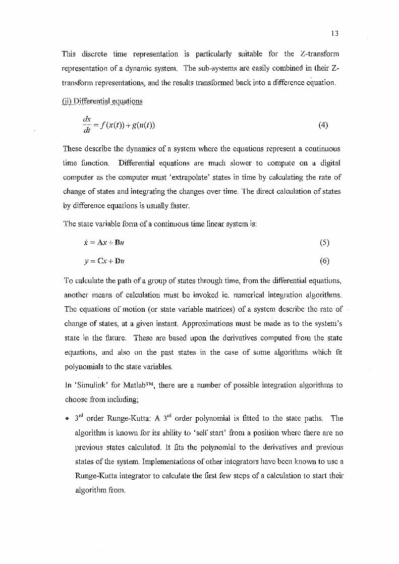
0) Difference equations
x(k+ 1) ~ f(x(k)) + g(u(lc)) (1)
These describe the next state in the time series, as a function of it's previous states and
it's inputs. Difference equations are fast to compute on digital computers as the nature
of the calculations lend themselves to high speed matrix manipulation (the realm of the
digital signal processing chip or DSP). The sampled data state variable fonn of a
linear system is:
(2)
(3)
13
This discrete time representation 1S particularly suitable for the Z-transform
representation of a dynamic system. The sub-systems are easily combined in their Z
transform representations, and the results transformed back into a difference equation.
(ii) Differential eguations
d'C -d = f(x(t)) + g(u(t))
t (4)
These describe the dynamics of a system where the equations represent a continuous
time function. Differential equations are much slower to compute on a digital
computer as the computer must 'extrapolate' states in time by calculating the rate of
change of states and integrating the changes over time. The direct calculation of states
by difference equations is usually faster.
The state variable form of a continuous time linear system is:
x = Ax+Bu
y = Cx+Du
(5)
(6)
To calculate the path of a group of states through time, from the differential equations,
another means of calculation must be invoked ie. numerical integration algorithms.
The equations of motion (or state variable matrices) of a system describe the rate of
change of states, at a given instant. Approximations must be made as to the system's
state in the future. These are based upon the derivatives computed £i'om the state
equations, and also on the past states in the case of some algorithms which fit
polynomials to the state variables.
In 'Simulink' for Matlab™, there are a number of possible integration algorithms to
choose from including;
® 3rd order Runge-Kutta: A 3rd order polynomial is fitted to the state paths. The
algorithm is known for its ability to 'self start' from a position where there are no
previous states calculated. It fits the polynomial to the derivatives and previous
states of the system. Implementations of other integrators have been known to use a
Runge-Kutta integrator to calculate the first few steps of a calculation to start their
algorithm from.
14
@ sth order Runge-Kutta: A sth order polynomial is fitted to the state paths. This
algorithm has the same features as the 3rd order Runge-Kutta but uses the higher
order polynomial fit.
I) Euler: This simple method uses the state equations in the first two terms of the
Taylor series:
(7)
As the Euler method is a relatively fast algorithm to calculate, it was typically
used to perform a brief trial simulation of a model to ascertain the stability and
validity of the numerical model before performing a simulation using a more
complex (and slower) algorithm such as the 3rd order Runge-Kutta.
• Adams-Gear: A predictor-corrector algorithm which uses two previous time steps
to calculate a polynomial fit to the state paths.
Each integrator has it's peculiarities and sensitivities to the system of equations it is
being used to solve. With some models, the results for a lmown stable system can
become quite badly unstable forcing the supervisory software to halt the simulation.
This may be as a result of poor choice of time step, or because the integrator has too
great (or small) a range of time steps to operate within. Computation time increases
with O(1/n), where n is the time step, so n'is usually made a large as possible and
model is designed to minimise needless calculation.
Choosing appropriate time steps can be left to the integration algorithm. The
algorithms used by Simulink have the advantage of incorporating adaptive time steps
which adjust with the rates of change of the system being simulated. If the system
states change quic1dy with time, the algorithm chooses a smaller time step to increase
the resolution at that time. Conversely it will increase the time step if the system
changes slowly with time.
After determining the system's equations of motion the plant model can be represented
by its equations of state. These can also be convelted to transfer functions where
required.
15
2.2 DERIVATION OF THE AGV MODEL
In order to simulate the AGV system, a numerical representation or 'model' had to be
created that represented the dynamics of the AGY. This section describes the process
of developing such a model of the AGY.
2.2.1 Notation
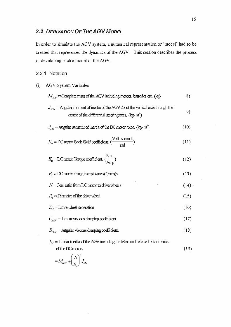
(i) AGV System Variables
~GV = Complete mass of the AGV including motors, batteries etc. (kg)
JAGV = Angular moment of inertia of the AGV about the vertical axis through the
centre of the differential steering axes. (kg· m2)
J r:c = Angular moment of inertia of the DC motor rotor. O(g' m2)
Volt· seconds I~ = DC motor BackEMF coefficient. ( d )
N'm Ke = DC motor Torque crefficient. (Amp)
Rc = DC motor annaLure resistance (Olnns)s
ra
N = Gear ratio from DC motor to drive vmeels'
R..v = Diameter of the chive wheel
Llv = Dtive vmee1 separation
CAGV = linear viscous damping coefficient
BAGV = Angular viscous damping coefficient.
Ilot = linear inertia ofthe AGV including the J'vlass and referred polar ine1tia
of the DC motors
~~cv+(j' J",
8)
9)
(10)
(11)
(12)
(13)
(14)
(15)
(16)
(17)
(18)
(19)
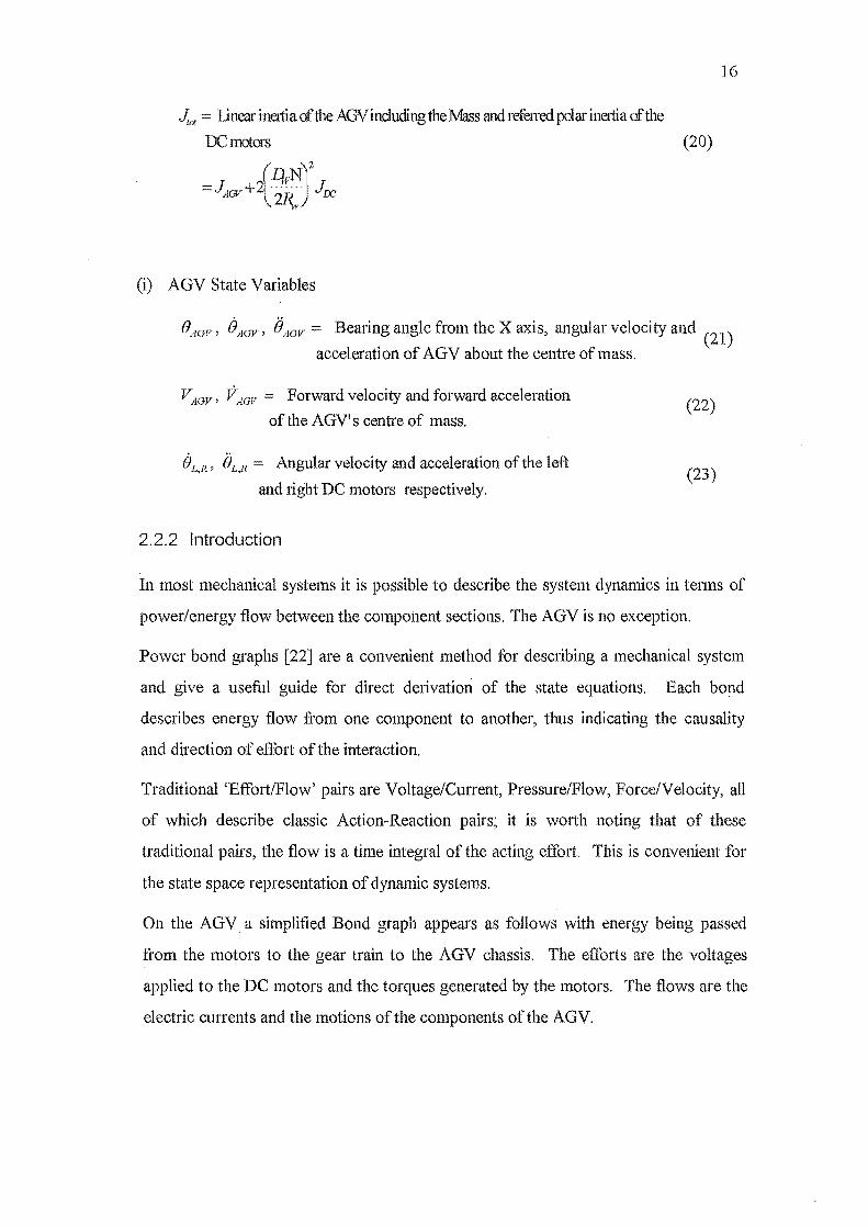
~ot linear inertia of the AGVincluding the l\1ass and referred polar inertia of the
DCn'Dtors
(i) AGV State Variables
16
(20)
8AGV ' OAGV' (j AGV Bearing angle from the X axis, angular velocity and (21)
acceleration of AGV about the centre of mass.
VAGV ' VAGV Forward velocity and forward acceleration
of the AGV's centre of mass.
OL,R' 0L,R Angular velocity and acceleration of the left
and right DC motors respectively.
2.2.2 Introduction
(22)
(23)
In most mechanical systems it is possible to describe the system dynamics in terms of
power/energy flow between the component sections. The AGV is no exception.
Power bond graphs [22] are a convenient method for describing a mechanical system
and give a useful guide for direct derivation of the state equations. Each bond
describes energy flow from one component to another, thus indicating the causality
and direction of effort ofthe interaction.
Traditional 'Effort/Flow' pairs are Voltage/Current, Pressure/Flow, Force/Velocity, all
of which describe classic Action-Reaction pairs; it is worth noting that of these
traditional pairs, the flow is a time integral of the acting effort. This is convenient for
the state space representation of dynamic systems.
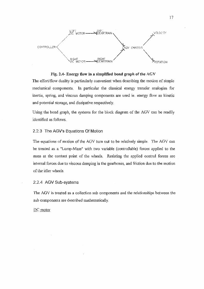
On the AGV a simplified Bond graph appears as follows with energy being passed
from the motors to the gear train to the AGV chassis. The efforts are the voltages
applied to the DC motors and the torques generated by the motors. The flows are the
electric currents and the motions of the components of the AGV.
17
LEFT LEFT /DC MOTOR --" ..... ""IICEARTRAIN '" /ELOCITY
CONTROLLER\ )GV CHASSIS
~ROTATIO' Fig. 2.4- Energy flow in a simplified bond graph of the AGV
The effortlflow duality is particularly convenient when describing the motion of simple
mechanical components. In particular the classical energy transfer analogies for
inertia, spring, and viscous damping components are used ie. energy flow as kinetic
and potential storage, and dissipative respectively.
Using the bond graph, the systems for the block diagram of the AGV can be readily
identified as follows.
2.2.3 The AGV's Equations Of Motion
The equations of motion of the AGV turn out to be relatively simple. The AGV can
be treated as a "Lump-Mass" with two variable (controllable) forces applied to the
mass at the contact point of the wheels. Resisting the applied control forces are
internal forces due to viscous damping in the gearboxes, and fnction due to the motion
of the idler wheels.
2.2.4 AGV Sub-systems
The AGV is treated as a collection sub components and the relationships between the
sub components are described mathematically.
DC motor
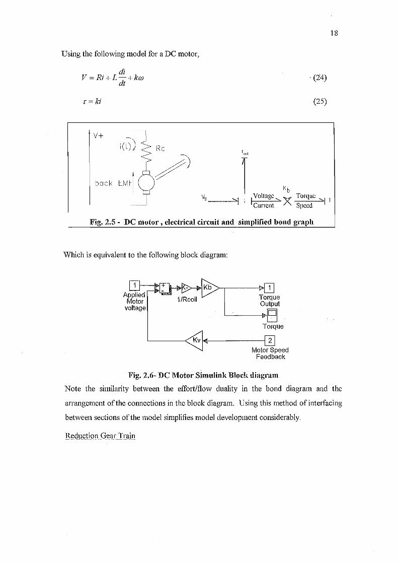
Using the following model for a DC motor,
di V = Ri + L dt + k(()
r=ki
v+ i(0} Rc rcoil
I Kb Vs ....... . Voltage ....... X ---""II I I Current
18
. (2'4)
(25)
Torque ....... 1 T Speed
Fig. 2.5 - DC motor, electrical circuit and simplified bond graph
Which is equivalent to the following block diagram:
>-r----{;9OJ Torque Output
'--------p.-B Torque
14------[I] lVlotor Speed
Feedback
Fig. 2.6- DC Motor Simulinl{ Block diagram
Note the similarity between the effortlflow duality in the bond diagram and the
arrangement of the connections in the block diagram. Using this method of interfacing
between sections of the model simplifies model development considerably.
Reduction Gear Train
19
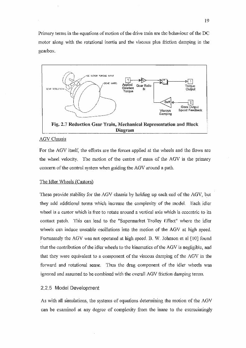
Primary terms in the equations of motion of the drive train are the behaviour of the DC
motor along with the rotational inertia and the viscous plus friction damping in the
gearbox.
DC MOTOR TOROUE INPUT
RIVE WHEEl
GEAR KLUU'C IIUN"
Gear Ratio N
Q----!OJ Torque Output
1+---10 GboxOu!put
Viscous Speed Feedback Damping
Fig. 2.7 Reduction Gear Train, Mechanical Representation and Block Diagl'am
AGV Chassis
For the AGV itself, the efforts are the forces applied at the wheels and the flows are
the wheel velocity. The motion of the centre of mass of the AGV is the primary
concern of the control system when guiding the AGV around a path.
The Idler Wheels (Castors)
These provide stability for the AGV chassis by holding up each end of the AGV, but
they add additional terms which increase the complexity of the model. Each idler
wheel is a castor which is fTee to rotate around a vertical axis which is eccentric to its
contact patch. TIns can lead to the "Supermarket Trolley Effect" where the idler
wheels can induce unstable oscillations into the motion of the AGV at high speed.
Fortunately the AGV was not operated at high speed. B. W. Johnson et al [10] found
that the contribution of the idler wheels to the kinematics of the AGV is negligible, and
that they were equivalent to a component of the viscous damping of the AGV in the
forward and rotational sense. Thus the drag component of the idler wheels was
ignored and assumed to be combined with the overall AGV friction damping terms.
2.2.5 Model Development
As with all simulations, the systems of equations determining the motion of the AGV
can be exannned at any degree of complexity from the inane to the excruciatingly
20
triviaL Relevant non-linearities were included as the model was developed from the
most simple case.
Using only integration operations wherever possible reduces numerical stability
problems when computing the system dynamics. Numerically calculated derivatives
can cause instabilities in the solution if the time steps are not appropriately chosen.
Also, the use ofthe lis operator maintains consistency with the state variable approach
to matrix representation of the AGV model.
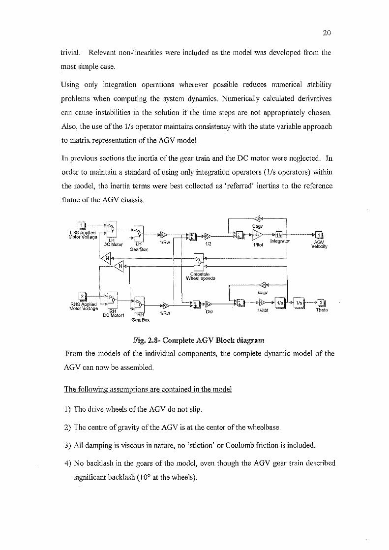
In previous sections the inertia of the gear train and the DC motor were neglected. In
order to maintain a standard of using only integration operators (lis operators) within
the model, the ineltia terms were best collected as 'referred' inertias to the reference
fi'ame of the AGV chassis.
GearBox
Calculate Wheel speeds
Fig. 2.8- Complete AGV Bloch: diagram
From the models of the individual components, the complete dynamic model of the
AGV can now be assembled.
The following assumptions are contained in the model
1) The drive wheels of the AGV do not slip.
2) The centre of gravity of the AGV is at the center of the wheelbase.
3) All damping is viscous in nature, no 'stiction' or Coulomb fhction is included.
4) No backlash in the gears of the model, even though the AGV gear train described
significant backlash (100 at the wheels).
2.3 DETERMINING SYSTEM PROPERTIES USING SYSTEM
iDENTIFICA TlON METHODS
21
Within the dynamics of the AGV were a number of sub-systems with unknown co
efficients and properties. These included, the behaviour of the DC motor, and most
importantly, the behaviour of the DCMC. In order to control the AGV properly it
would be preferable to know the dynamics of these sub systems, but determining these
dynamics is an interesting problem. One approach would be to give the AGV known
inputs and determine the order and amplitude of the dynamics by examination, relying
on the experience ofthe observer to estimate the dynamics implicitly.
However rather than rely solely on the interpretation of the results by an observer, it
was decided to attempt to determine these sub-systems by means of systems
identification techniques.
The problem of system identification is to estimate a model of a system based on input
and output data, and a priori knowledge of the possible nature of the dynamics of the
system. As the DCMC, and the dynamics of the power transmission system were the
main unknown areas of the AGV, they were investigated using the following methods.
The core of the System Identification Toolbox is the representation of a model, or
system of equations, as a discrete time sequence. The Matlab tool used in this analysis
was the least squares error approximation tool (pEM.M). A complete description of
the parameter process can be found in L. Ljung[16].
The observer treats the unknown system as a 'black box' (a convenient notation in the
case of the DCMC as it was a black box), feeds measured demands to the system, and
records the outputs. The Matlab 'System ill' toolbox takes care of most of the
computational detail, and the observer is fi'ee to examine a number of proposed
models. The problem can them become one of model reduction, or what order of
model best represents the dynamics being examined.
The solution of a system model is an iterative process involving the presentation,
calculation and evaluation of candidate models based on the systems I/O data gained
from experiments. Experiments must be appropriately designed (where possible) to
isolate or exaggerate the desired dynamic effects.
22
THE EXPERIMENTS:
A number of experiments were performed in order to isolate the dynamics of the target
systems. In the case of the AGV , it is relatively simple to isolate the sub-systems from
the AGV and examine them individually. In a more complex system tIus would not
necessarily be possible.
2.4.1 Recording the dynamics of the DCMC and gear train
The AGV was raised off the ground, allowing the drive wheels to rotate freely. The
DCMC input section was attached to the microcontroller.
In all cases a Universal Pulse Processor (UPP) card (Hitaclu HD64130) was used in
the host PC to measure both the analog demand signals from the micro controller, and
the speed of the DC motors whlch was inferred from attached position encoders.
The following methods were used to generate the demand signals:
1. A program written in C running on the microcontroller was used to generate signals
of pseudo-random pulse length and intervals. These ±100% demand signals were
sent to the DCMC.
2. Used a free standing joystick to generate a random input pattern to the DCMC, the
operator moved the joystick in the most random manner that could be managed:
Test lUns lasted fi'om 2-15 seconds and the results of which were recorded in the
memory of the a host PC. After the test was completed, the data was written to a file
for later analysis with Matlab.
From the presentation of the data of the tests above, a number of models were
fonnulated for the dynamics of the DCMC.
(l) The first proposed model for the DCMC is a simple gain matrix taldng two
signals representing forward and turn demand, and converting them into left and right
wheel speeds by varying the voltage applied to the wheels. Simple DC motor theory
will set the wheel speed to a given value for a voltage (at a given load).
(2) The second model presumes that the DCMC has some measure of feedback
logic and can vary the output voltage to achieve the required wheel speed. The exact
measure of this feedback is unknown so two possibilities are proposed:

23
1. Simple Proportional gain
II. Proportional + Integral gain.
From the results obtained, the DCMC could incorporate either model (1) or (II), as
there was no compelling evidence for a more complex control strategy being used in
the DCMC.
NOTE: The experiments were not originally designed to perform the analysis of the
second option. To obtain better results in determining the operation of the DCMC,
another scheme would be needed. Using an intermediate voltage measurement level it
is then possible to determine the voltage applied to the motors by the DCMC, rather
than attempting to imply the operation of the DCMC from the motion of the wheels.
2.4.2 Recording and analysis of the Electric Motors and drive train
From the equations of motion of a simple DC motor, the dynamics of an electric motor
are determined by the following co~efficients.
Kv = coefficient of proportionality of back - EMF
from shaft rotational speed
La = DC motor coil inductance
R" DC motor armature resistance
J DC polar moment of inertia of the rotor
(26)
(27)
(28)
(29)
Certain constants in the drive motors were unknown, the inertia and viscous friction of
the DC motor rotor, the brush friction and the Kv constant of proportionality for
calculating the back EMF from the motor speed. With the exception of the motor coil
inductance, these values are quite crucial to the AGV model dynamics.
24
DC Motor
'I'I'---,OUADRATURE ENCODER
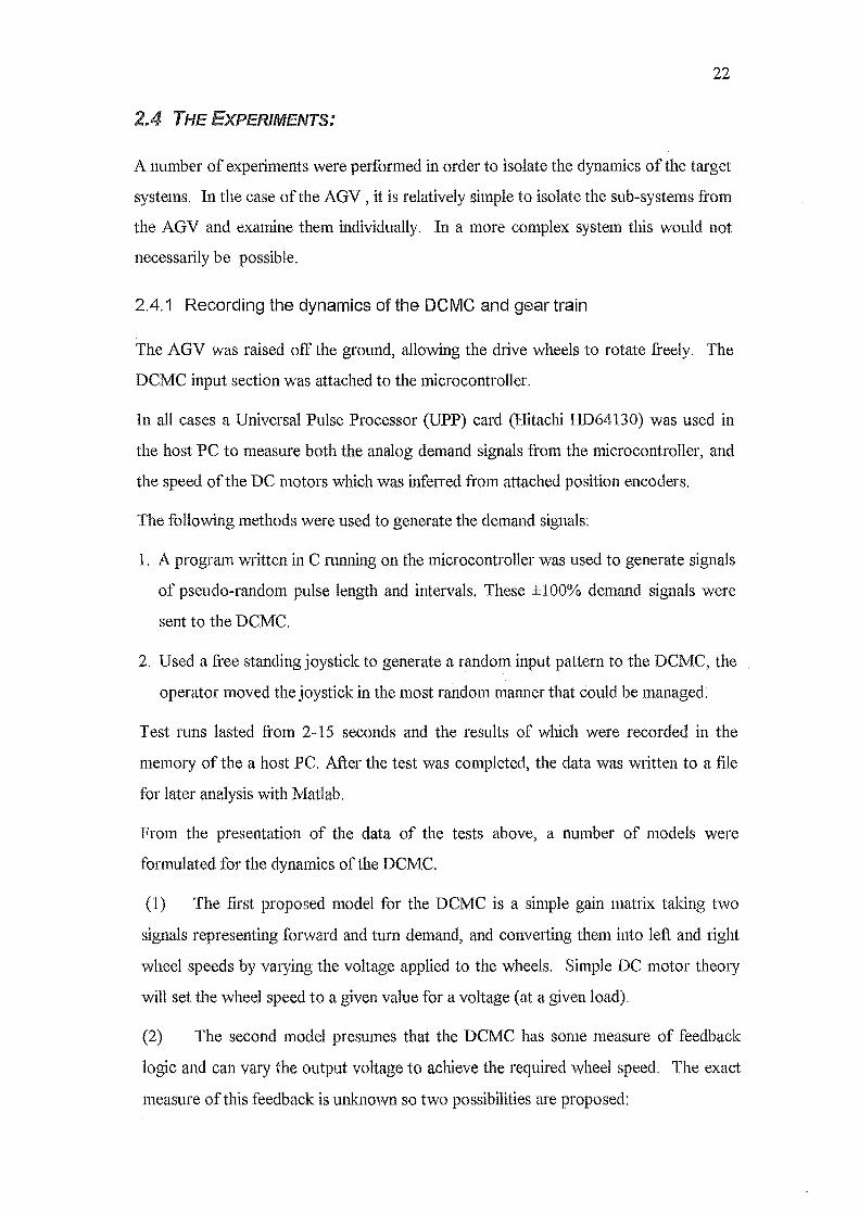
Fig. 2.9~ Bad" EMF, DC motor rotor inertia test rig.
In order to find the polar moment of inertia of the DC drive motors, they were
removed from the AGV and quadrature rotary encoders were attached to the output
shaft. A pulley was attached to the motor output shaft and a weight was hung off the
pulley at table height.
The weight was dropped from table height, and the UPP card was used to measure the
timing pulses from the encoders, and the back EJVIF generated across the motor
terminals at speed. A number of different weights were used. This data was recorded
and saved to file for later analysis.
To attempt to measure the viscous damping of the DC motors rotor, the AGV was
lifted off the ground (fully assembled) and the electric motors were driven at full speed
by connecting the motor terminals directly across the drive batteries. With the motor at
full speed, the power was removed, and the wheels were left to coast to a stop under
the effects of whatever clamping was present. The motor speed and input voltage were
measured and recorded with time.
2.4.3 Recording the performance of the AGV under closed loop control
Measuring the performance of the AGV, the data of interest is the path of the AGV
with respect to the guide wire during closed loop control. A number of methods were
considered to measure the actual performance of the AGV under closed loop control.
These included:
25
L Data logging from extra sensors to perform 'dead-reckoning'. For example adding
position encoders to each wheel to measure the speed, and calculating the position
of the AGV over time by integrating the encoder records.
II. By attaching cables to stationary points, and calculating the position of the AGV
from triangulation of the cable lengths to the AGV. TIns method could also
provide an instantaneous direction vector by adding a position encoder to one of
the cables at the AGV.
IILDirect measurement of the AGV position by means of a pigment trace on paper.
(effectively using the AGVas a 120kg 'Logo' turtle)
Method I would suffer from integration and quantisation errors over time. Imai et a1
[13J state that open ended dead reckoning (without any means of calibration with the
real world position) has limited range, and becomes less accurate with the increasing
distance travelled. Also, dead reckoning is dependant on a no-slip condition ie.
constant wheel speed with AGV speed, or complex modelling of the slip functions, c.f.
A. Hamdy and E. Badreddin [5]. Wheel slip will introduce errors into the position
calculation that would be magnified with subsequent readings. Even though the AGV
models assume no-slip at the drive wheels (in fact wheel slip was observed on
occasion). There is no way to guarantee thls in the actual AGV without additional
engineering ie. adding position sensors to the idler wheels. This reliance on the no-slip
condition meant that the dead reckOlnng method was unacceptable.
Method II was too complicated and costly to implement when compared with the
other options.
,-' \ \
AGV Chassis member '. \ \ \
Felt tipped pen~ \ \~\
Solenoi I I '. I
\ \ , \ I\.. _
_ ... _ ... __ :~L_i. -\ \ -,,- --..- \ \\
---- \ \\ I I,
'. '. " , . . .' . .
" ..,Jl .. .. <I ~ ..
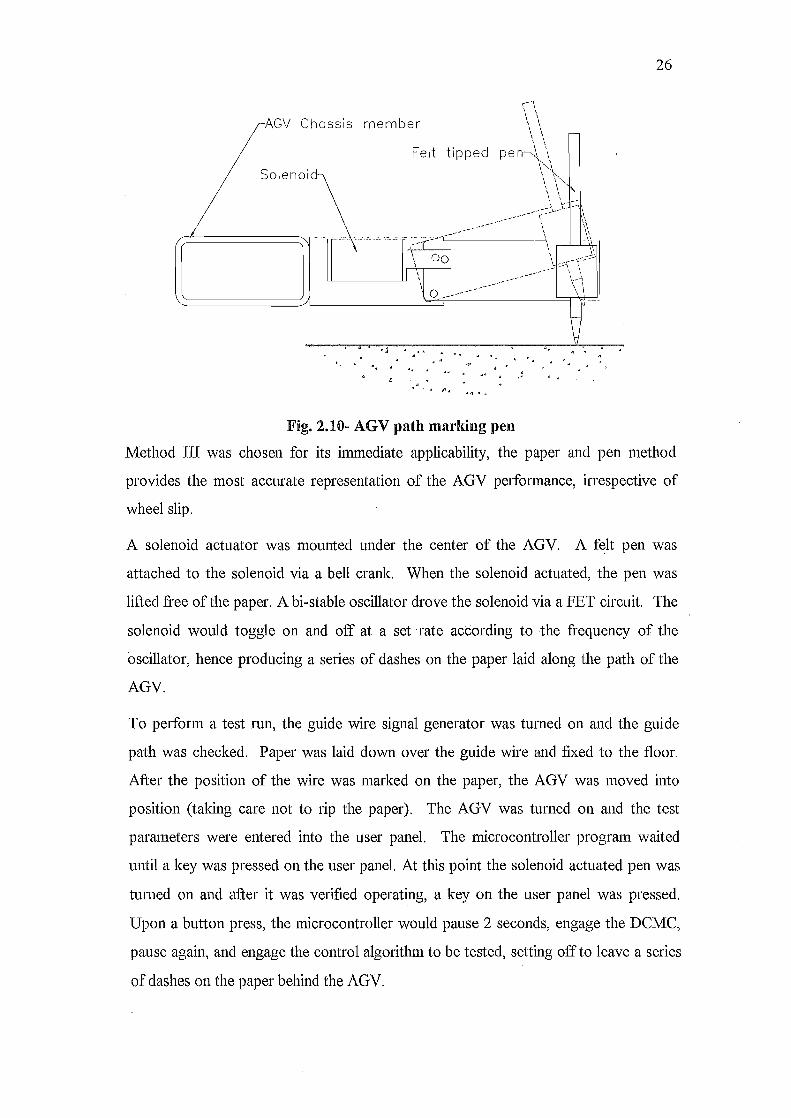
Fig. 2.10- AGV path marldng pen
26
Method III was chosen for its immediate applicability, the paper and pen method
provides the most accurate representation of the AGV performance, irrespective of
wheel slip.
A solenoid actuator was mounted under the center of the AGY. A felt pen was
attached to the solenoid via a bell crank. When the solenoid actuated, the pen was
lifted free of the paper. A bi-stable oscillator drove the solenoid via a FET circuit. The
solenoid would toggle on and off at a set 'rate according to the frequency of the
oscillator, hence producing a series of dashes on the paper laid along the path of the
AGY.
To perform a test run, the guide wire signal generator was turned on and the guide
path was checked. Paper was laid down over the guide wire and fixed to the floor.
After the position of the wire was marked on the paper, the AGV was moved into
position (taldng care not to rip the paper), The AGV was turned on and the test
parameters were entered into the user panel. The micro controller program waited
until a key was pressed on the user panel. At this point the solenoid actuated pen was
turned on and after it was verified operating, a key on the user panel was pressed.
Upon a button press, the microcontroller would pause 2 seconds, engage the DCMC,
pause again, and engage the control algorithm to be tested, setting off to leave a series
of dashes on the paper behind the AGY.
27
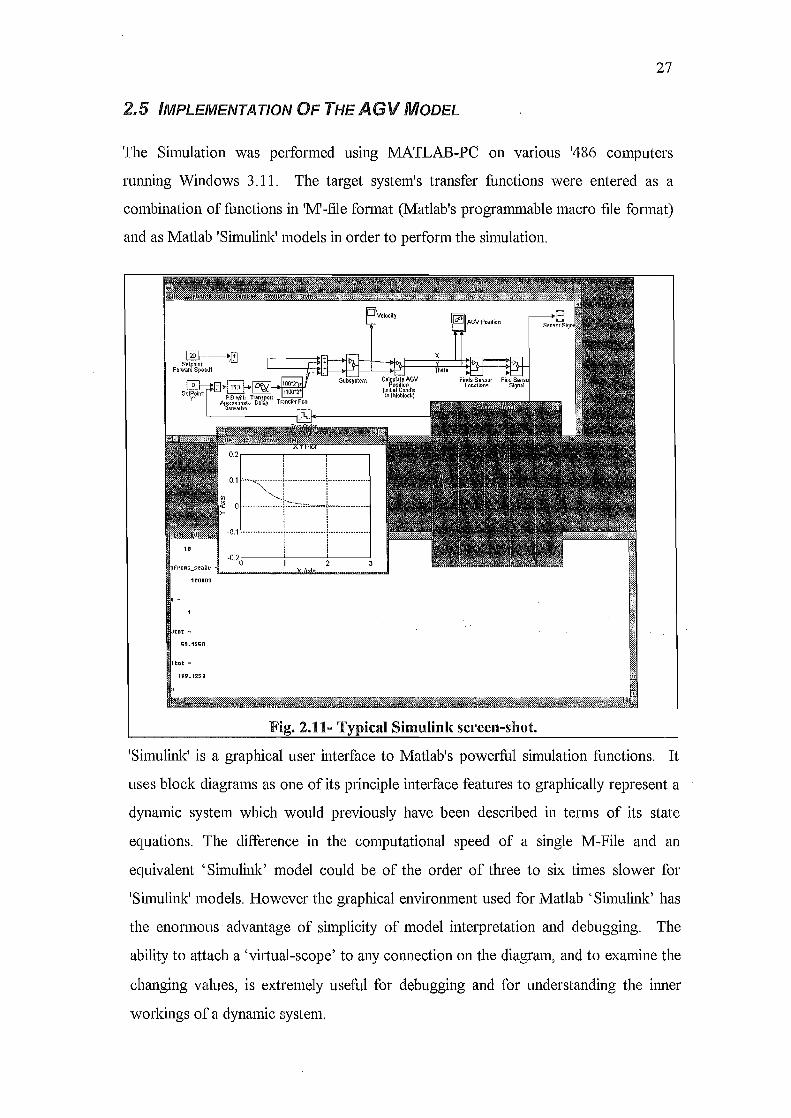
2.5 IMPLEMENTATION OF THE AGV MODEL
The Simulation was performed using MATLAB-PC on vanous '486 computers
mnning Windows 3.11. The target system's transfer functions were entered as a
combination of functions in 'M'-file format (Matlab's programmable macro file format)
and as Matlab 'Simulink' models in order to perfonn the simulation.
11J1l1IllO
50.1250
to:l: =
199.1250
, , I !
0.1 " .. ~:.-.-------i--- ..... -....... i.-............. .
"»t~~c+-·0.'1 ················i················j················ : :
l ! .0.20'-------':--->-------'
1 Simulink screen-shot.
'Simulink' is a graphical user intelface to Matlab's powerful simulation functions. It
uses block diagrams as one of its principle interface features to graphically represent a
dynamic system which would previously have been described in terms of its state
equations. The difference in the computational speed of a single M-File and an
equivalent 'Simulink' model could be of the order of three to six times slower for
'Simulink' models. However the graphical environment used for Matlab 'Simulink' has
the enormous advantage of simplicity of model interpretation and debugging. The
ability to attach a 'virtual-scope' to any connection on the diagram, and to examine the
changing values, is extremely useful for debugging and for understanding the inner
workings of a dynamic system.
28
The 'Simulink' model of the AGV was developed through the following stages of
complexity.
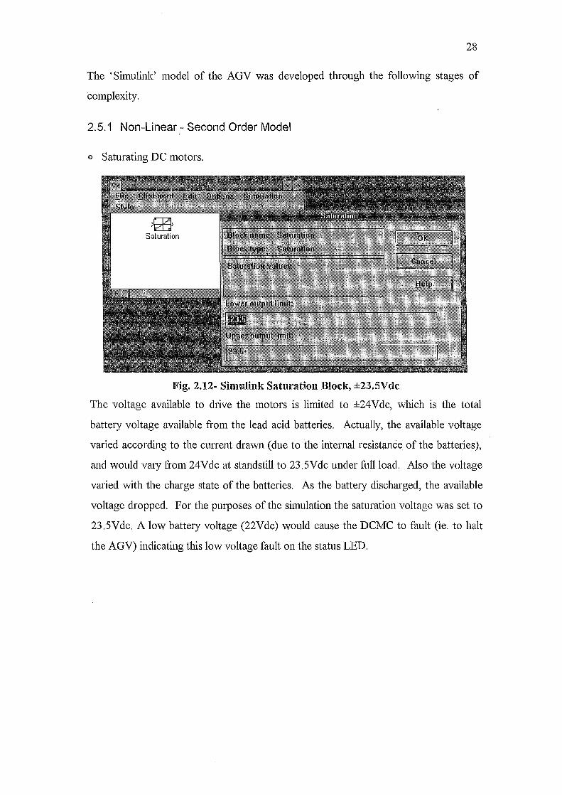
2.5.1 Non-Linear - Second Order Model
III Saturating DC motors.
Fig. 2.12~ Simulink Saturation Block, ±23.5Vdc
The voltage available to drive the motors is limited to ±24Vdc, which is the total
battery voltage available from the lead acid batteries. Actually, the available voltage
varied according to the current drawn (due to the internal resistance of the batteries),
and would vary from 24Vdc at standstill to 23.5Vdc under full load. Also the voltage
varied with the charge state of the batteries. As the battery discharged, the available
voltage dropped. For the purposes of the simulation the saturation voltage was set to
23.5Vdc. A low battery voltage (22Vdc) would cause the DCMC to fault (ie. to halt
the AGV) indicating this low voltage fault on the status LED.
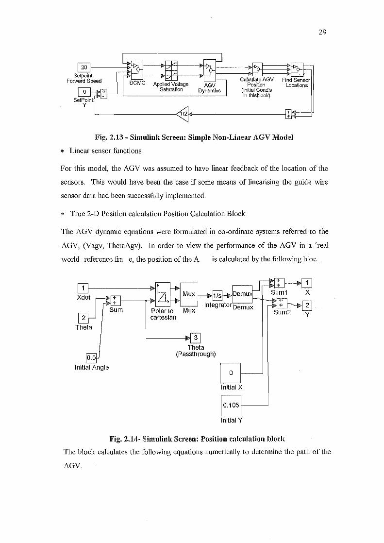
S~I-t: --"'rEf---""":m-:*-t-----.,r--' j--~O-I--"I Forward Speed DCMC Calculate AGV Find Sensor
Applied Voltage AGV Position Locations Saturation Dynamics (Initial Cond's
in thisblock)
"-----------<1/2l<1li----'-----------1 t l4--+,
Fig. 2.13 - Simulinh: Screen: Simple Non-Linear AGV Model
• Linear sensor functions
29
For this model, the AGV was assumed to have linear feedback of the location of the
sensors. This would have been the case if some means of lineadsing the guide wire
sensor data had been successfully implemented.
€) True 2-D Position calculation Position Calculation Block
The AGV dynamic equations were formulated in co-ordinate systems referred to the
AGV, (Vagv, ThetaAgv). In order to view the performance of the AGV in a 'real
world reference fra e, the position of the A is calculated by the following bloc
[IJI---------i X;ndot .,.,[]
Sum 2
Theta
Initial Angle
'------B>I 3
Theta (Passthrough)
~[JJ Sum1 X
[]~~{~J Sum2 y
a
Initial X
O. 1 05 f-------.J
Initial Y
Fig. 2.14- Simulink Screen: Position calculation blod{
The block calculates the following equations numedcally to determine the path of the
AGV.
T
X = Xo + f v cos(O+ 00 ) ·dt o
T
Y = Yo + f V sine 0 + 00 ) • dt o
where (xo ,Yo, 00 ) are the initial conditions:
e = V = 0, at T = O.
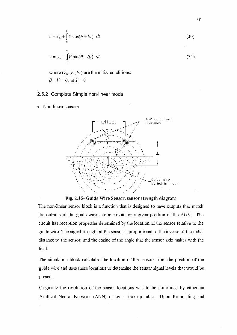
2.5.2 Complete Simple non-linear model
(l) Non-linear sensors
wire
Guide Wil'e Buried ill Flool-
Fig. 2.15- Guide 'Wire Sensor, sensor strength diagram
30
(30)
(31)
The non-linear sensor block is a function that is designed to have outputs that match
the outputs of the guide wire sensor circuit for a given position of the AGY. The
circuit has reception properties determined by the location of the sensor relative to the
guide wire. The signal strength at the sensor is proportional to the inverse of the radial
distance to the sensor, and the cosine of the angle that the sensor axis makes with the
field.
The simulation block calculates the location of the sensors £l'om the position of the
guide wire and uses these locations to determine the sensor signal levels that would be
present.
Originally the resolution of the sensor locations was to be performed by either an
Artificial Neural Network (ANN) or by a look-up table. Upon formulating and
31
training ( off line) a neural network to perform the function inversion, it was found that
the computational overhead for a Neural Network on the given micro controller was
such that it would only be capable of performing a position calculation 4 tunes every
second. This was unacceptable, and rather than re~code it to some faster method (it
involved re-writing large sections of the floating point math librruy in either fixed point
or integer math) it was decided to discard this method. Upon closer examination of
the sensor function, there is more than one point on the curve where the sensor values
are the same for different locations. Thus a look-up table was not very reliable.
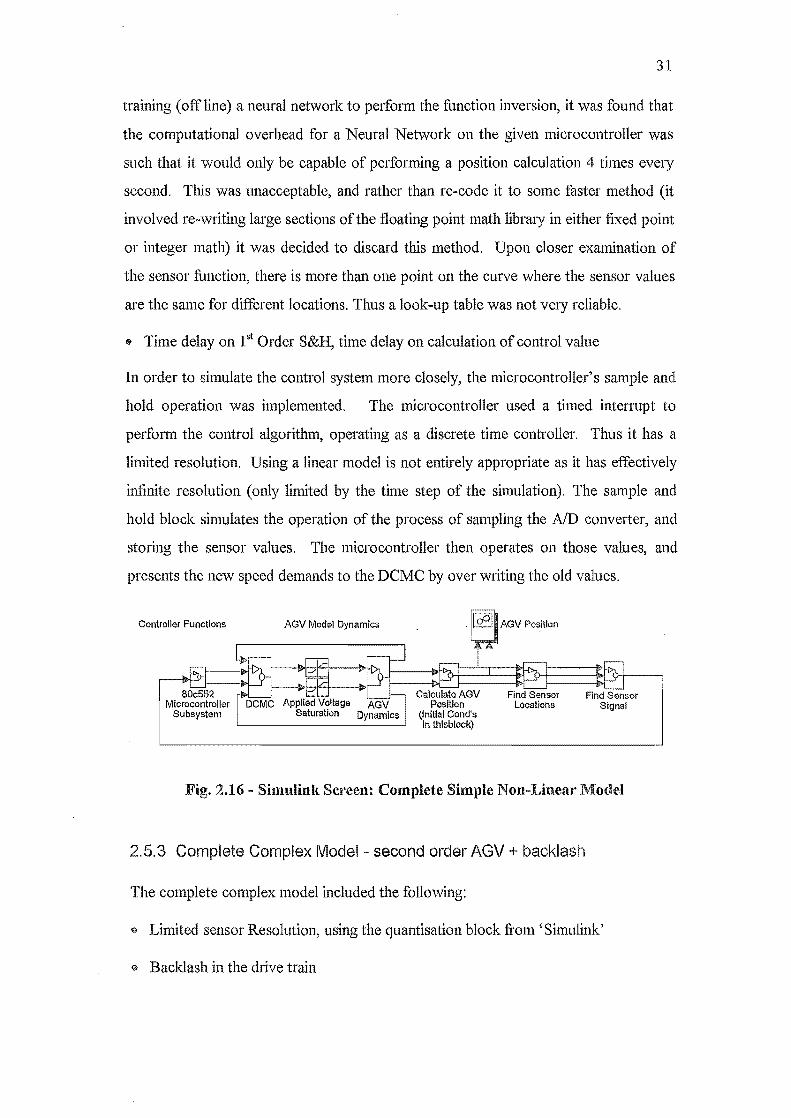
o Time delay on 1st Order S&H, time delay on calculation of control value
In order to simulate the control system more closely, the micro controller' s sample and
hold operation was implemented. The micro controller used a timed interrupt to
perform the control algorithm, operating as a discrete time controller. Thus it has a
limited resolution. Using a linear model is not entirely appropriate as it has effectively
infinite resolution (only limited by the time step of the simulation). The sample and
hold block simulates the operation of the process of sampling the AID converter, and
storing the sensor values. The micro controller then operates on those values, and
presents the new speed demands to the DCMC by over writing the old values.
Controller Functions AGV Model Dynamics
Fig. 2.16 - Simulink Screen: Complete Simple Non-Linear 'Model
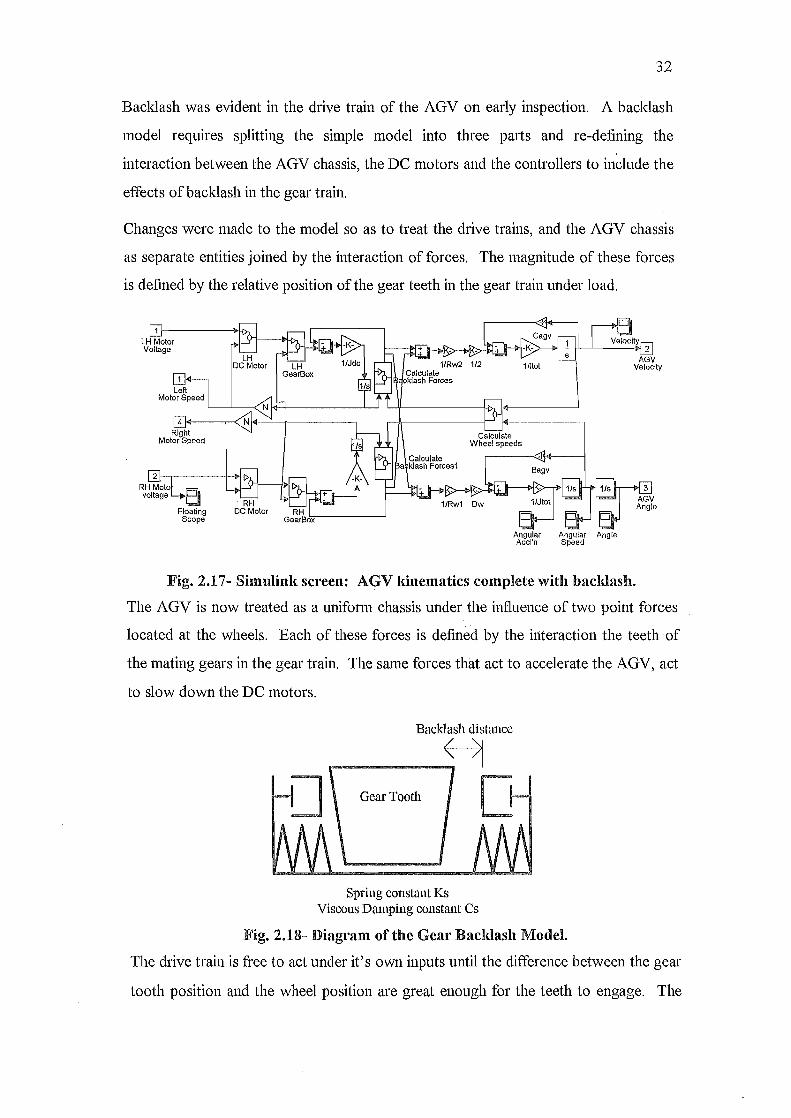
2,5.3 Complete Complex Model- second order AGV + backlash
The complete complex model included the following:
o Limited sensor Resolution, using the quantisation block from' Simulink'
@ Backlash in the drive train
32
Bacldash was evident in the drive train of the AGV on early inspection. A backlash
model requires splitting the simple model into three parts and re-defining the
interaction between the AGV chassis, the DC motors and the controllers to include the
effects of bacldash in the gear train.
Changes were made to the model so as to treat the drive trains, and the AGV chassis
as separate entities joined by the interaction of forces. The magnitude of these forces
is defined by the relative position of the gear teeth in the gear train under load.
[JJ-----~f>, LH Motor Voltage
11l<l----.-< Right
Motor Speed
1/2 1/ltot
Calculate Wheel speeds
Calculate ~<t a klash Fore~~~~~~gv 1/s
Ow 1/Jtot
o Angular Angular Angle Acel'n Speed
Fig. 2.17- Simulink screen: AGV l{inematics complete with bacldash.
The AGV is now treated as a uniform chassis under the int1uence of two point forces
located at the wheels. Each of these forces is defined by the interaction the teeth of
the mating gears in the gear train. The same forces that act to accelerate the AGV, act
to slow down the DC motors.
Backlash distance
Gear Tooth
Spring constant Ks Viscous Damping constant Cs
Fig. 2.18- Diagram of the Gear Bacldash Model.
The drive train is free to act under it's own inputs until the difference between the gear
tooth position and the wheel position are great enough for the teeth to engage. The
33
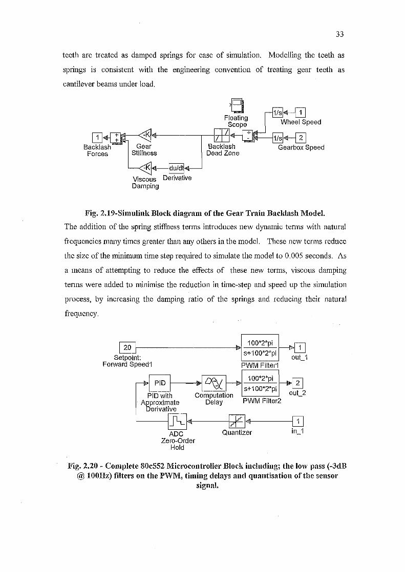
teeth are treated as damped springs for ease of simulation. Modelling the teeth as
springs is consistent with the engineering convention of treating gear teeth as
cantilever beams under load.
OJ Backlash Forces
Viscous Derivative Damping
>8 Floating Scope
Backlash Dead Zone
1/s~ Wheel Speed
fM--l1/s ~-QJ Gearbox Speed
Fig. 2.19-Simulinh: Bloch: diagram of the Gear Train Bacldash Model.
The addition of the spring stiffness terms introduces new dynamic terms with natural
frequencies many times greater than any others in the model. These new terms reduce
the size of the minimum time step required to simulate the model to 0.005 seconds. As
a means of attempting to reduce the effects of these new terms, viscous damping
terms were added to minimise the reduction in time-step and speed up the simulation
process, by increasing the damping ratio of the springs and reducing their natural
frequency.
20 ---------.~I ~11l ~ 100*2*pi s+100*2*pi I ",-~
Setpoint: out_1 FOlward Speed1 PWIVI Filter1
I I I L---... 100*2*pi
PID f------D>1ie> ~ 1~1Ji" s+100*2*pi PID with Computation
Approximate Delay PWM Filter2 Derivative
f----~<t4--[JJ Quantizer in_1 ADC
Zero-Order Hold
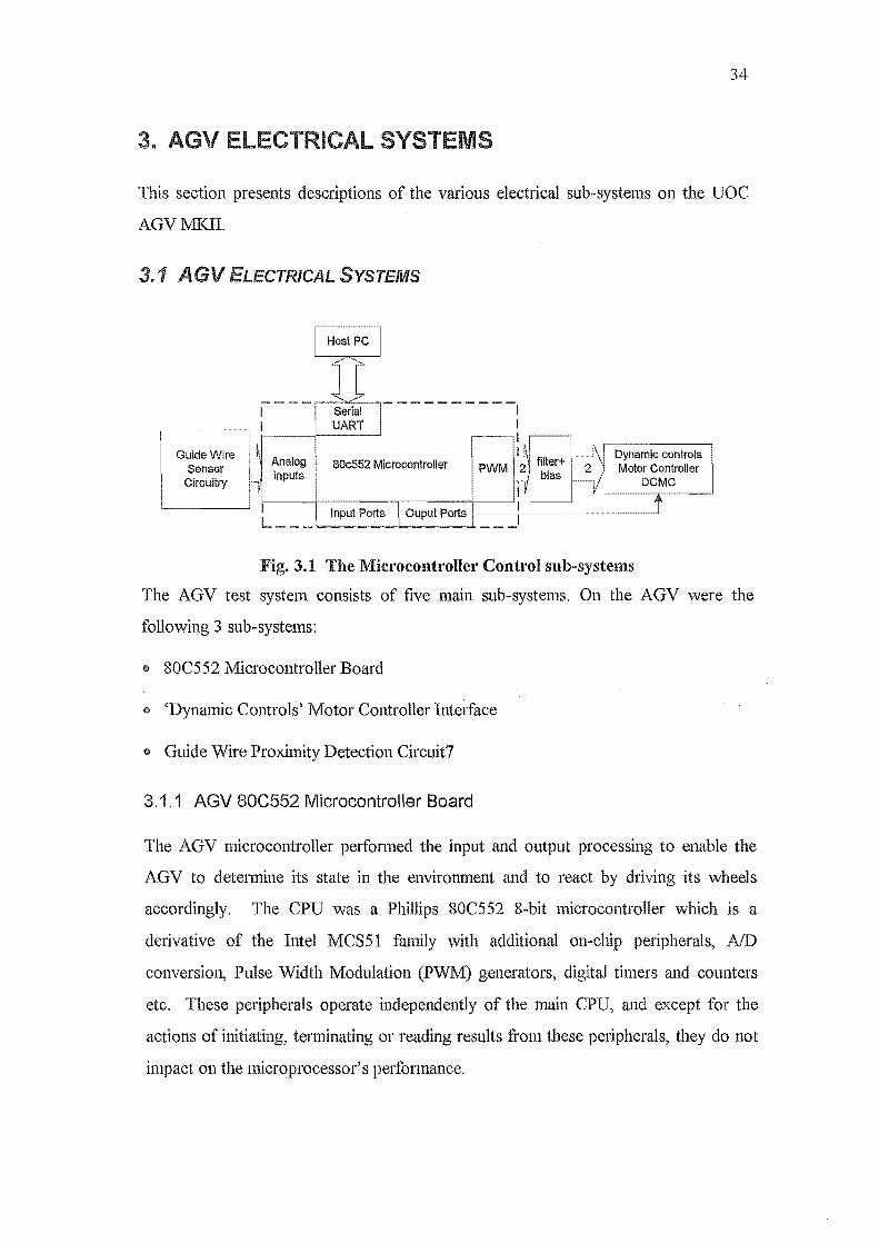
Fig. 2.20 - Complete 80c552 Microcontroller Blocl{ including; the low pass (-3dB @ 100Hz) filters on the PWlVI, timing delays and quantisation of the sensor
signal.
34
3. AGV __ .... SySTEMS
This section presents descriptions of the various electdcal sub-systems on the UOC
AGVMKII.
3.1 AGV ELECTRICAL SYSTEMS
----------1
Guide Wire Sensor
Circuitry
Analog 80c552 Mlcrocontroller Inputs '
1 1
Fig. 3.1 The Micl'oColltrollel' Control sub-systems
The AGV test system consists of five main sub-systems. On the AGV were the
following 3 sub-systems:
(!) 80C552 Microcontroller Board
~ 'Dynamic Controls' Motor Controller Inteiface
I» Guide Wire Proximity Detection Circuit7
3.1.1 AGV 80C552 Microcontroller Board
The AGV microcontroller performed the input and output processing to enable the
AGV to determine its state in the environment and to react by driving its wheels
accordingly. The CPU was a Phillips 80C552 8-bit micro controller which is a
derivative of the Intel MCS51 family with additional on-chip peripherals, AID
conversion, Pulse Width Modulation (PWM) generators, digital timers and counters
etc. These peripherals operate independently of the main CPU, and except for the
actions of initiating, terminating or reading results from these peripherals, they do not
impact on the microprocessor's pelformance.
3S
The micro controller was purchased complete as a development board for application
testing and included an on board monitor program in EPROM for interfacing with a
host computer via a serial communications port. This monitor program was later
replaced by a more complicated 'C' debugger/monitor called the 'Lucifer Debugger'
from HiTech Software.
An elementary user intelface was added to the AGV. It consisted of an LCD display
(20 character x 2 line array) and an array of push buttons. By means of the AGV user
interface, control variables could be changed without the need to reconnect the AGV
to it's support PC.
The micro controller memory map consisted of 8k RAM and 8Ic ROM mapped into the
same address space. The architecture of the 80cS1 family of micro controllers has
separate program and data spaces. This feature is appropriate for commercial
applications where the product's program is static, but it is not appropriate for code
development. In order to program new code into RAM to be executed, the memory
spaces had to be re-mapped to coincide by digital logic ('OR'ing PSEN and RD) in
external circuitry. Thus programs could be read and written to high address data
("RAM") blocks which were also mapped as low address program ("ROM") blocks.
The microcontroller intelfaces with a number of small peripheral circuits which were
driven by the dedicated circuits on the microcontroller. The internal PWM circuit was used to generate an analog signal via a filter circuit. This analog voltage to the DCMC
was used to indicate the Forward/Turn speeds.
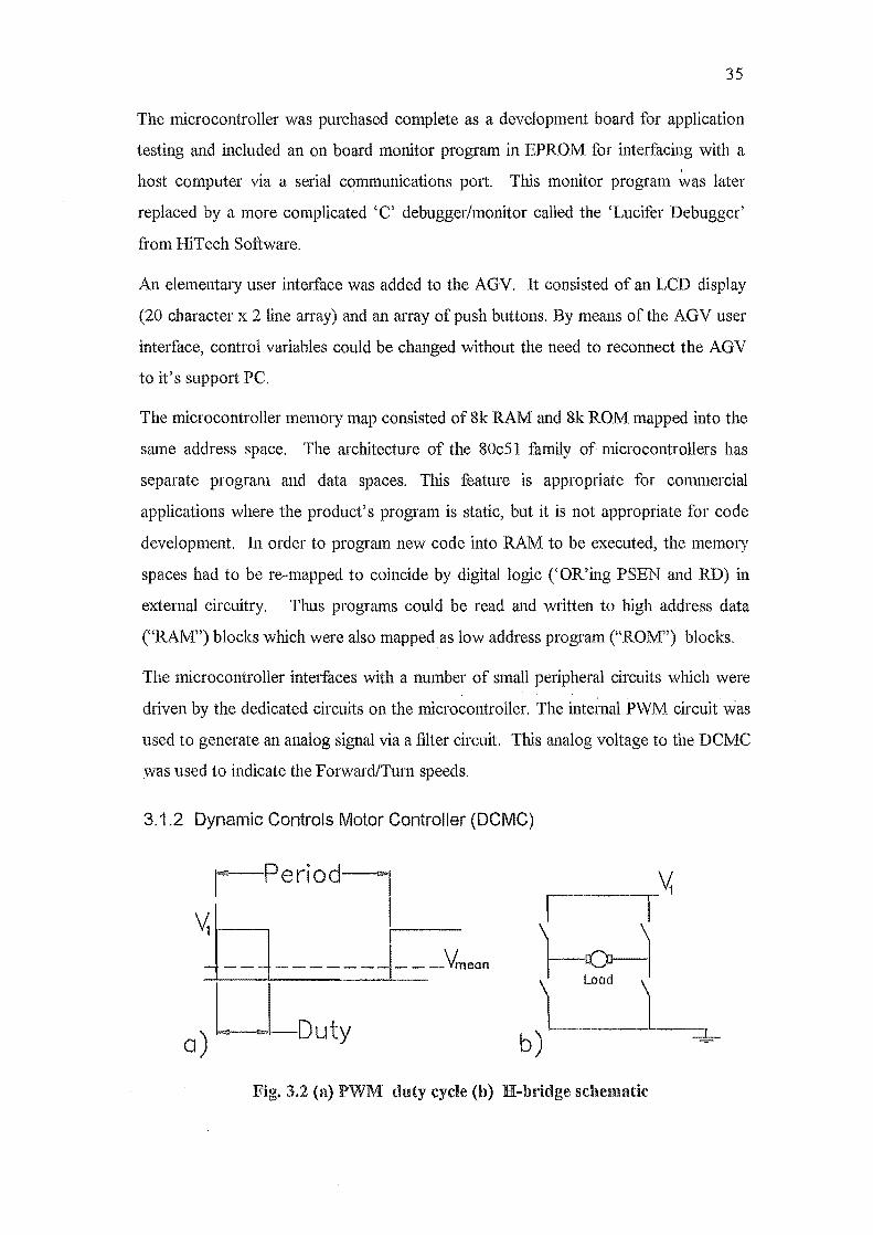
3.1.2 Dynamic Controls Motor Controller (DCMC)
Fig. 3.2 (a) PWM duty cycle (b) H-hddge scbematic
36
The DCMC is essentially a microprocessor controlled pair ofH-bridge circuit drivers.
It has circuitry to maintain and monitor the speed of the wheelchair motors to which it
is usually attached. The exact circuitry of the DCMC is a commercial secret and is not
available. The DCMC allows proportional speed control of the motors by means of
PWM switching of the four arms of the H bridge. By switching quicldy between 'on'
and 'off' states, the mean voltage applied to the motor is propoliional to the mean 'on'
time of each PWM cycle.
The DCMC used a single input as an 'enable'. Failure to assert this input would
engage a 'braking' mode to bring the AGV to a stop and attempt to hold the wheels
stationary. From experience pushing the AGV from point to point between test runs,
the resistance to motion was significantly greater when the DCMC was engaged than
when it was off. This meant that the DCMC gave substantially better braking
pelformance under the control of the DCMC than by simply removing the power (as
was done to test the stopping distance for the bumpers).
As the DCMC was designed to control a wheelchair, it exhibited a number of
operational 'quirks' which were necessarily accommodated for in the microcontroller
program. If the DCMC received a non-zero demand signal in the first :h second after
tliggering the enable, the controller would fault. This 'feature' was to prevent a
wheelchair occupant from removing the park-brake and immediately going into
motion, possibly injuring themselves in the process. As well, the microcontroller had
limits to the demand signals it would accept. A combination of high forward speed
demand, and high turn speed demand would cause the DCMC to indicate a fault and
bring the motors to a stop. This prevents the wheelchair pilot being thrown out during
a high speed turn. Thus speed must be reduced for sharp turns.
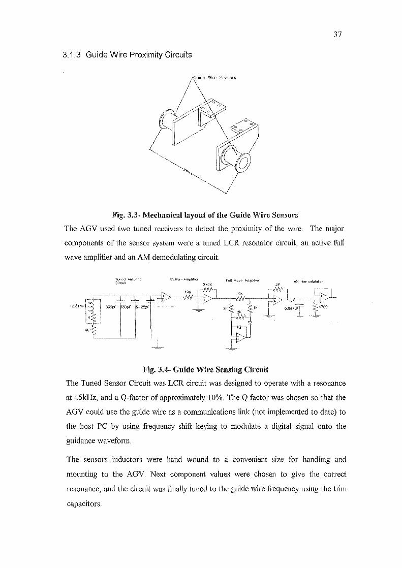
37
3.1.3 Guide Wire Proximity Circuits
Fig. 3.3- Mechanicallayout of the Guide '''ire Sensors
The AGV used two tuned receivers to detect the proximity of the wire. The major
components of the sensor system were a tuned LCR resonator circuit, an active full
wave amplifier and an AM demodulating circuit
Tuned Antenna (In::;uil
Buifer-Amplifier full wave Amplifier 270K
Fig. 3.4~ Guide Wire Sensing Circuit
21(
The Tuned Sensor Circuit was LCR circuit was designed to operate with a resonance
at 45kHz, and a Q-factor of approximately 10%. The Q factor was chosen so that the
AGV could use the guide wire as a communications link (not implemented to date) to
the host PC by using frequency shift keying to modulate a digital signal onto the
guidance waveform.
The sensors inductors were hand wound to a convenient Size for handling and
mounting to the AGV. Next component values were chosen to give the COlTect
resonance, and the circuit was finally tuned to the guide wire frequency using the trim
capacitors.
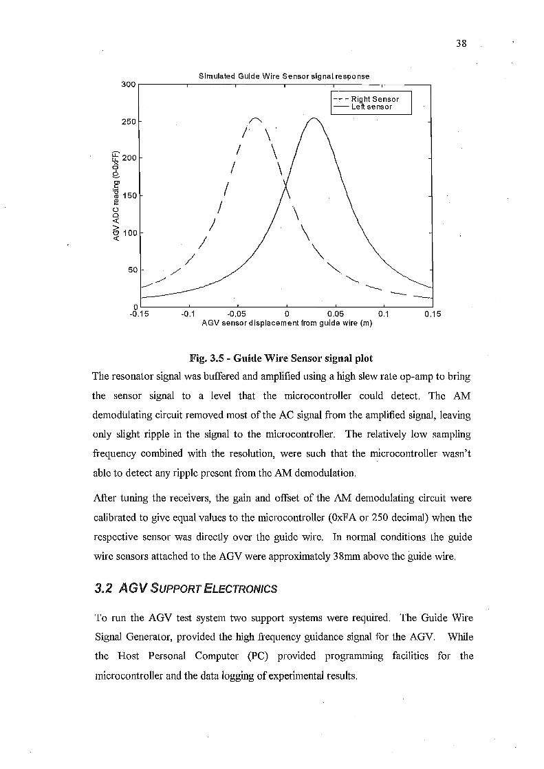
Simulated Guide Wire Sensor signal response 300,-------.-------.-------,--------.-------.-------,
250
G:' 200
i ~ 'g 150 II:! () o « ~ 100 «
50
----
,/ /.
/ /
/
/"'-
/' /
/ I
/ \ \
\
-'e - Right Sensor - Left sensor
~. ~
o~------~------~------~------~------~------~ -0.15 -0.1 -0.05 0 0.05 0.1 0.15
AGV sensor displacement from guide wire (m)
Fig. 3.5 - Guide Wire Sensor signal plot
38
The resonator signal was buffered and amplified using a high slew rate op-amp to bring
the sensor signal to a level that the micro controller could detect. The AM
demodulating circuit removed most of the AC signal from the amplified signal, leaving
only slight ripple in the signal to the micro controller. The relatively low sampling
frequency combined with the resolution, were such that the microcontroller wasn't
able to detect any ripple present from the AM demodulation.
After tuning the receivers, the gain and offset of the AM demodulating circuit were
calibrated to give equal values to the micro controller (OxFA or 250 decimal) when the
respective sensor was directly over the guide wire. In normal conditions the guide
wire sensors attached to the AGV were approximately 38mm above the guide wire.
3.2 AGV SUPPORT ELECTRONICS
To run the AGV test system two support systems were required. The Guide Wire
Signal Generator, provided the high frequency guidance signal for the AGY. While
the Host Personal Computer (PC) provided programming facilities for the
micro controller and the data logging of experimental results.
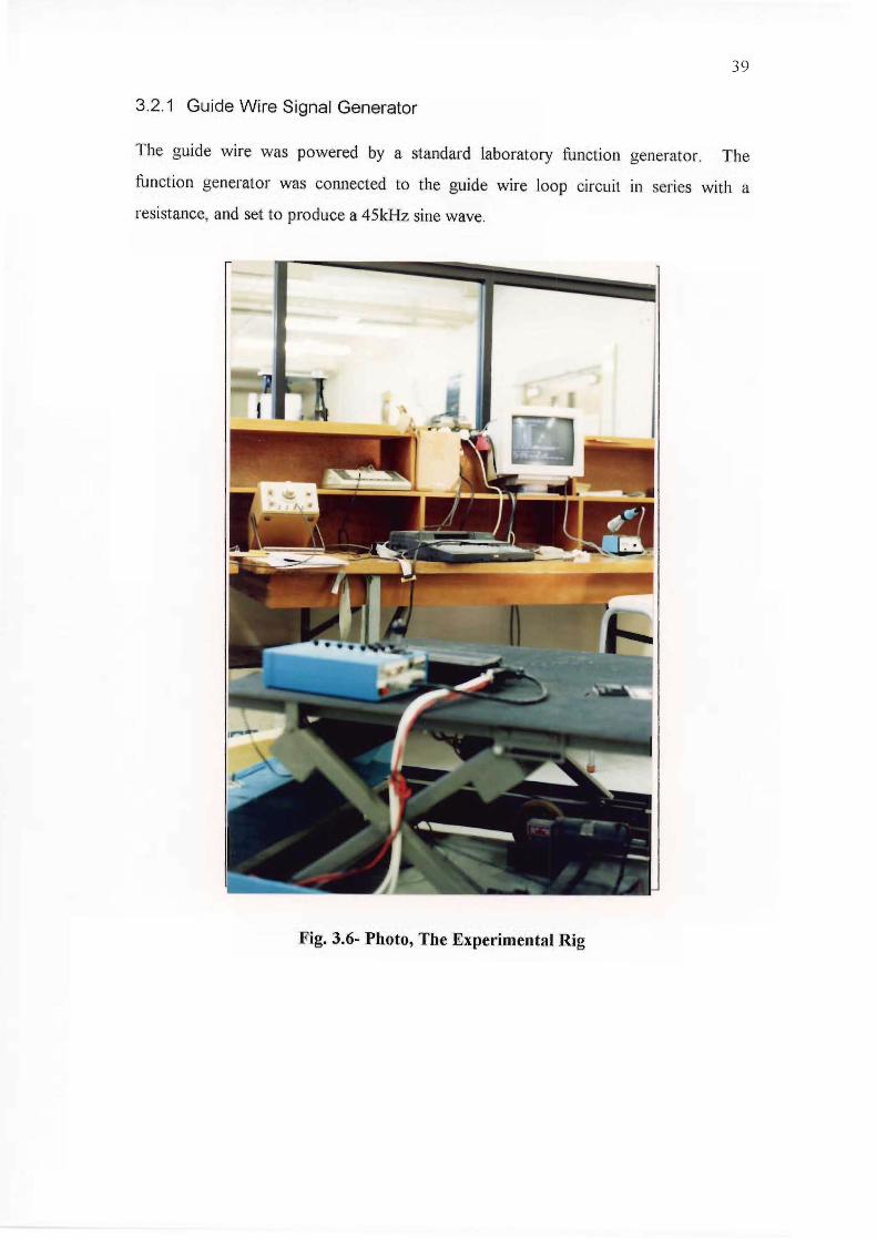
39
3.2.1 Guide Wire Signal Generator
The guide wire was powered by a standard laboratory function generator. The
function generator was connected to the guide wire loop circuit in series with a
resistance, and set to produce a 45kHz sine wave.
Fig. 3.6- Photo, The Experimental Rig
40
3.2.2 Host PC
An IBM-PC compatible computer was equipped with software and hardware, in order
to program the microcontroller and to perform data recording for the system
identification experiments.
The Universal Pulse Processor Card (UPP Card) was an ISA-bus card designed as a
signal processing peripheral for the IBM-PC (c.f G.R. Dunlop et al [21]). Past
applications of the card have included; Fuzzy Logic control of an invetied pendulum,
real time optimal control of a hydraulic cylinder (c.f Steve Hampson [1]), position
control of a prosthetic finger (c.f Derek Ward [17]).
The UPP has digital pulse processing capabilities as well as AID conveliers. The pulse
processing circuitry is programmable, in that a dedicated controller on the card
(I-litachi Part #HD64130) can be programmed to execute simple macro functions to
registers on the chip. Programming libraries written by Andy Creel and Julian Murphl
allowed an easy interface to the UPP for accessing the registers.
On the AGV project the UPP's digital pulse processing functions were primarily used
to log speed and position information from quadrature encoders, and to generate
timing pulses for other data logging operation. The encoders used were 2 channel 256
count per revolution quadrature encoders, giving 1024 position counts per revolutioti.
The UPP's analog inputs were used variously to measure analog voltages from the
AGV, the demand signals to the DCMC, and the back EMF generated by the each DC
motor. In each case, the voltages in the experiment were scaled to fit into the range of
the AID converters on the UPP by using simple OP-AMP circuits.
1 Teclmician in charge of DOC Robotics and Applied Mechanics laboratories, PhD candidate
1'eclmician in charge of DOC Electronics and Computer workshop
41
4. AGV PROJ SOFTWARE
During the course of the project, a number of computer programs were written to
control the AGV and it's SUppOlt systems. This section describes the software that was
used to write these programs, and the programs that were written.
4.1 MICRO CONTROLLER PROGRAMMING SOFTWARE
A number of languages were considered to program the microcontroller, including
variants of 'Forth', 'Modula-2' and 'C'.
Assembly language was initially considered, but the lack of familiarity with the 80c552
made that option inefficient. The assemblers evaluated were mostly free-ware or
share-ware, and mostly missing any facility for linking multiple files into a single block
of machine code for execution. However over the duration of the project, a great
many opportunities to become :familiar with 80cS1 assembly code presented
themselves. These arose from the need to de-bug and evaluate code generated by the
various compilers.
Dynamic Controls Ltd provided a copy of 'Mod51' a commercial 'Modula-2' package
designed for the 80cS1 family of microprocessors. This package was used in the first
stages of software development, however it soon proved to be more difficult to use
than was anticipated. The compiler generated extremely bulky code in certain
circumstances, and the syntax of the 'Modula-2' language was restrictive compared to
'C'. The author was initially unfamiliar with 'Modula-2', and sought opinions of the
'Mod-51' compiler from more experienced 'Modula-2' programmers. The consensus
view was that this implementation was incomplete in terms of it's functionality and
lack of adherence to the de-facto industry standards. Henceforth, in concert with
another project in progress within the department, a 'c' development suite was
purchased.
The 'HiTech -C' development suite consisted of the usual bevy of 'c' tool including
pre-processor, linker, and an Integrated Development Environment (IDE). As well, it
included an extension to the IDE in the form of a program to download software to a
target system, and debug the users 'C' source code. This program, 'The Lucifer
42
Debugger' (LUC51.EXE), used the serial port of the PC to communicate to a
micro controller running the 'Lucifer target'. This enabled the programmer to step
through the 'c' program running on the microcontroller, and see the corresponding
section of code on the PC screen. The 'Lucifer Target' was a monitor program stored
in EPROM on the target microcontroller. On the AGV the 'Lucifer Target' program
replaced the standard development EPROM supplied by the development board
manufacturer (Phillips).
When the microcontroller booted, the program would test the status of one of the
input lines. Depending on the state of this line, it would either execute the 'Lucifer
Target' or a program stored in user RAM. A section of code would be loaded into
RAM on the Microcontroller, debugged using the 'Lucifer' and then the
microcontroller would be re-booted after switching the 'UserlMonitor' switch to
'User'. Upon a hard RESET the micro controller would execute the user code in
RAM, ignoring the 'Lucifer' code.
4.2 HOST PC SUPPORT SOFTWARE
The software to pelform data-logging of the AGV for the System Identification
experiments, was written using 'Borland-C++ V1.0' and the UPP libraries written by
Andy Cree and Julian Murphy (See Section 3,2.2).
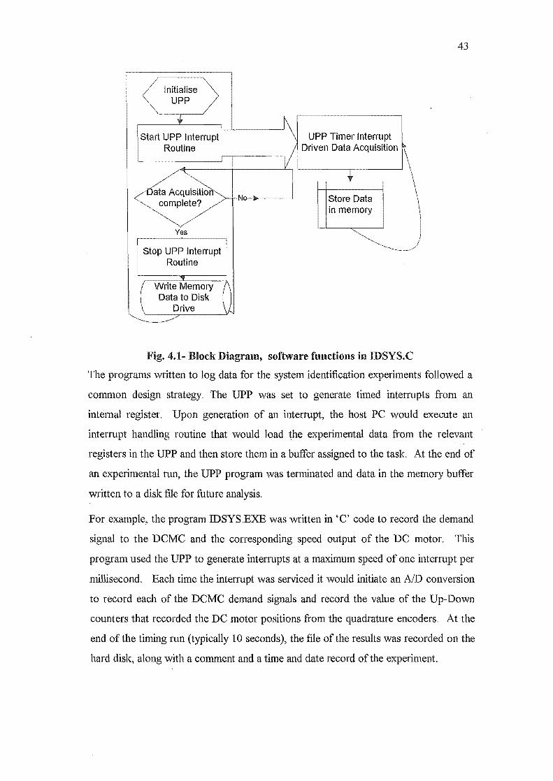
Initialise UPP
Start UPP Interrupt Routine
<' ata Acquisition " complete?
Yes
Stop UPP Interrupt Routine
Write Memory Data to Disk
Drive
upp Timer Interrupt Driven Data Acquisition
Store Data in memory
Fig. 4.1- Blocl{ Diagram, software functions in IDSYS.C
43
The programs written to log data for the system identification experiments followed a
common design strategy. The UPP was set to generate timed interrupts from an
internal register. Upon generation of an interrupt, the host PC would execute an
interrupt handling routine that would load the experimental data from the relevant
registers in the UPP and then store them in a buffer assigned to the task. At the end of
an experimental run, the UPP program was terminated and data in the memory buffer
written to a disk file for future analysis.
For example, the program IDSYS,EXE was written in 'C' code to record the demand
signal to the DCMC and the corresponding speed output of the DC motor. This
program used the UPP to generate intemlpts at a maximum speed of one interrupt per
millisecond. Each time the interrupt was serviced it would initiate an AID conversion
to record each of the DCMC demand signals and record the value of the Up-Down
counters that recorded the DC motor positions from the quadrature encoders. At the
end of the timing run (typically 10 seconds), the file of the results was recorded on the
hard disk, along with a comment and a time and date record of the experiment.
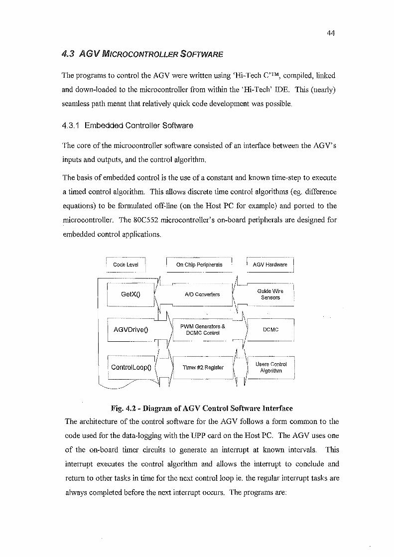
44
4.3 AGV MrCROCONTROLLER SOFTWARE
The programs to control the AGV were written using 'Hi-Tech C'TM, compiled, linked
and down-loaded to the micro controller from within the 'Hi-Tech' IDE. This (nearly)
seamless path meant that relatively quick code development was possible.
4.3.1 Embedded Controller Software
The core of the micro controller software consisted of an interface between the AGV's
inputs and outputs, and the control algorithm.
The basis of embedded control is the use of a constant and known time-step to execute
a timed control algorithm. This allows discrete time control algorithms (eg. difference
equations) to be formulated off-line (on the Host PC for example) and ported to the
micro controller. The 80C552 microcontroller's on-board peripherals are designed for
embedded control applications.
GetXO
AGVDriveO
I ControlLoopO I
On Chip periPher:l:l
AID Converters
PWM Generators & DCMC Control
Timer #2 Register
AGV Hardware
Users Control Algorithm
Fig. 4.2 - Diagram of AGV Control Software Intelface
The architecture of the control software for the AGV follows a form common to the
code used for the data-logging with the UPP card on the Host PC. The AGV uses one
of the on-board timer circuits to generate an interrupt at known intervals. This
interrupt executes the control algorithm and allows the interrupt to conclude and
return to other tasks in time for the next control loop ie. the regular interrupt tasks are
always completed before the next interrupt occurs. The programs are:
45
AGVLOOP.C : Uses on-board timer (TOC2) to generate timed intenupts to a service
routine. The service routine is vectored to the address of the users control code, as
defined in the arguments passed to the 'StartControlLoopO' function.
AGV AD.C : Retrieves the values of the ADC from the guide wire sensor inputs in
round robin fashion and stores the resultant values in the appropriate locations.
AGVPOS.C : Calculates the position of the AGY's Sensor from the sensor inputs
incident at the ADC.
AGVCONT.C : This module calculates the control signal to pass to AGVDRIVEO
from the position of the AGV calculated in AGVPOS.C.
AGVDRIVE.C : Performs the task of interfacing the users control code with the AGV
drive algorithms. The routines control and manage the drive status (Enabled or
Disabled) and the speed demand sent to the DCMC.
In general the software to control the DCMC via the microcontroller was developed
by trial and error in the laboratory. Simply put, an experimental methodology was
used to trial timing and demand limits to the DCMC in order to get the maximum
performance from the AGV without the DCMC faulting. Trial speed demands were
sent to the DCMC (with the wheels of the AGV safely off the ground) and limiting
demands were established. These limits were hard coded into the control software as
constants. Thus operating limits were established empirically which avoided
generating DCMC faults.
4.3.2 Utility and User Interface Software
In the main loop, the program sent status information to the LCD panel and
monitored the buttons for input. It also monitored the internal state of the AGV for
events such as collisions. The programs were:
AGVSER.C: Interfaces the user program with the on-chip UART. This section of
code provides elementary serial communications functions between the Host PC and
the micro controller. This module provides functions to send bits, bytes, and words as
decimal or hexadecimal.
46
AGVINT.C : This code module sets up the AGVs bumper safety interrupt. Upon
triggering by the AGV's bumper, the interrupt routine sets the DCMC speed demand
signals to zero (50% PWNI) and disables the drive.
The bumper interrupt operates on the XIRQ line to the micro controller, which is a
NOll-Maskable Interrupt (or NMI). This executes a jump to a routine which removes
the 'DriveEnabled' bit disabling the DCMC. The 'DdveEnabled' bit is a flag used to
indicate the status of the DCMC to the rest of the AGV software. It should only be
cleared by the bumper interrupt routine and written to by a Master Reset. This is
simply a software safety interlock. As such it should not be trusted in any other than a
controlled laboratory environment, as any errant code may accidentally ovelwrite the
wrong bits and send the AGV careering out of control. For commercial applications, a
hardware/hard-wired safety relay would remove power to the DCMC until the AGV is
reset by an authorised operator.
AGVV ARS.C : This module implements the variable adjustment program via the
keyboard and LCD screen on the AGV. It enables the user to change variables within
the program provided they are listed in the program at compile time.
The User interface routines provided the means for the operator to vary celiain
operating parameters within the AGY. Mostly, this consisted of maintaining the
control value coefficients. The user interface was wdtten so that the operator could
modify the numerator and denominator separately, so as to obtain practically any
coefficient that can be represented fractionally.
The 80C552 microcontroller can only perfonn 16 bit maths (fixed precision). The
simplest method for implementing fixed precision maths without increasing the
computational load on the CPU significantly by using a floating point library, is to use
a numerator and denominator value to represent a single fractional value. In this way
control values are calculated by first multiplying by the numerator, and then dividing
by the denominator.
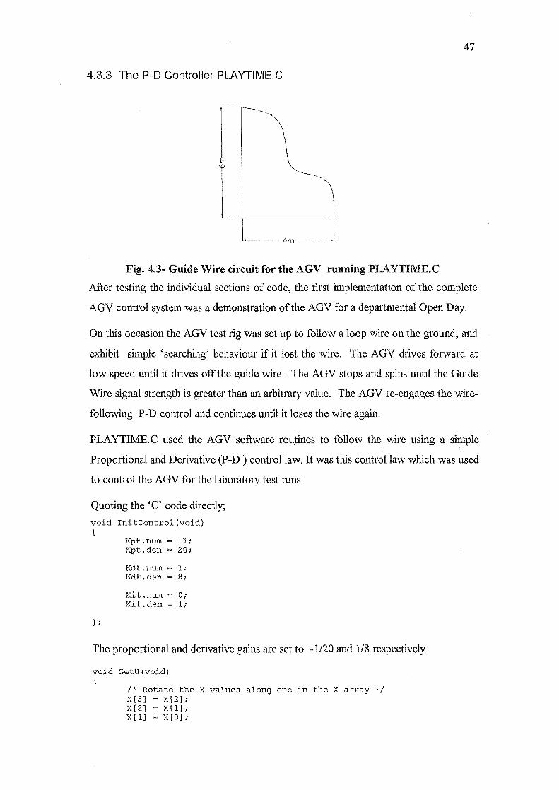
47
4.3.3 The P-D Controller PLAYTIIVIE.C
Fig. 4.3- Guide Wire circuit for the AGV running PLA YTIME.C
After testing the individual sections of code, the first implementation of the complete
AGV control system was a demonstration of the AGV for a departmental Open Day.
On tllis occasion the AGV test rig was set up to follow a loop wire on the ground, and
exhibit simple 'searc1ling' behaviour if it lost the wire. The AGV drives forward at
low speed until it drives off the guide wire. The AGV stops and spins until the Guide
Wire signal strength is greater than an arbitrary value. The AGV re-engages the wire
following P-D control and continues until it loses the wire again.
PLAYTIME. C used the AGV software routines to .follow the wire using a simple
Proportional and Derivative (P-D ) control law. It was this control law which was used
to control the AGV for the laboratory test runs.
Quoting the 'C' code directly;
void InitControl(void} {
} i
Kpt.num = -1; Kpt.den 20;
Kdt.nuro 1; Kdt.den = 8;
Kit.nuro = 0; Kit.den = 1;
The proportional and derivative gains are set to -1/20 and 1/8 respectively.
void GetU(void) {
/* Rotate the X values along one in the X array */ X[3] = X(2]; X[2] X(l] i X[l] X[O] i
} ;
X[O] = (Xpos);
/* Rotate the U values along one in the U array */ U[3] = U[2]; U[2] = U[I]; U[I] = U[O]; U [0] = UO;
48
UO.t = Kpt.num*(R.t - X[l]) / Kpt.den + Kdt.num*(X[O]-X[l])/Kdt.den; UO.f = R.f;
The previous control values are stored in a series of buffers. Before a new control
value is calculated, the old values are rotated forward in the arrays. This
implementation is relatively CPU intensive given that block move instructions such as
those found on the Z80 are not available on the MCSS1 microcontrollers. Also the
assembly code generated by the 'C' compiler for array manipulations is not compact.
A better implementation of this would be to use a circular buffer and use a single
pointer to the most recent value. If the buffer is 2N long (where N is an integer) and
starts at an address H where the lower N bits are zero, then an effective circular buffer
can be generated by always 'OR'ing any buffer address with H after setting the top
bits to zero. Thus if the address is incremented past the end of the buffer, the AND
00 .. 0011..1 (where there are N l's) followed by OR H (where there are NO's) always
puts the address pointer back to the start of the linear address block. Hence the
address scheme acts as a circular buffer. Note, ifH is all l's followed by NO's (ie. the
top 'page' of memory) then only the OR operation is required.
From these buffered control and sensor values, the P-D control algorithm calculates an
approximate derivative and a new control value.
5. RESULTS
EXPERIM
SYSTEM IDENTIFICATION
49
TIus section presents and exanlines the results of the experiments performed to analyse
the dynamics of the DCMC and the DC motors. The data was processed on Matlab,
and plots were generated comparing the simulated performance of the parameter
estimated models and the actual experimental data. To demonstrate these results a
typical series of plots is presented here, and a full summary of the data is given in the
appendices.
1 ANALYSING THE ELECTRIC MOTORS AND DRIVE TRAIN RECORDING
To measure the values of the AGV's physical properties, a number of short tests were
performed. These were described in Section 2.4.1. These results were used to
calculate the coefficient of the Back EMF, and also the rotational inertial of the rotor
for the DC motors.
Section 2.4.2 described the experiment to determine the Back EMF constant, and the
angular inertia of the DC motor. Examination of the plot of the angular velocity~vs
time graph in fig.5.l shows that the DC motor rotor accelerates until the weight hlts
the ground and then slows to a stop. The velocity of the DC motor under deceleration
shows an almost constant deceleration ie. none of the characteristics of a body under
viscous damping. The major braking force would seem to be a constant friction force
due to the bearings and the DC armature brushes.
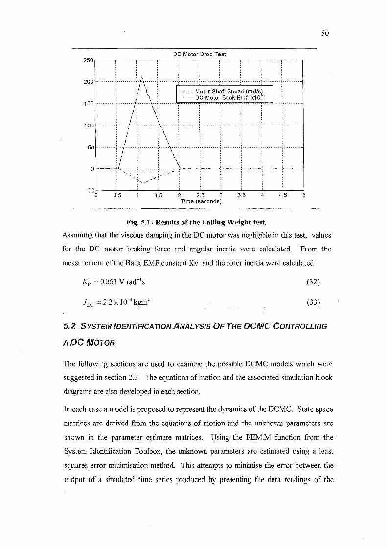
50
DC Motor Drop Test 250,---,----,----,----.---.----,----,----,---,----,
· . · . . ••••••• ~* ... *rr~ ........... _ ............... *~._ .......... ~ ...... ~ ___ .... .,.,.,~_ · . . 200 · . .
-.-.. - Motor Shaft Speed (rad/s) - DC Motor Back Emf (x1 00)
150 _ ................. .
· . . · . . 100 .......... 1' .......... : ........... [ .......... [ .......... \ .................. .
· . . · . . · . . 50 · . . . , •••. ' •• ~. ~ •••• _ ... -•••. _ ••• ... •• -••• -_. -~ ---_ ••..•.•.•• -• -_ .• - -» ---••. · , . . , · , . . . , , . . , · '; . , .. . , .. . · .. , , .. . · ., . · ., . .. . .. .
-50~--~--~----~---L--~----~--~----~--~--~
o 0.5 1.5 2 2.5 3 3.5 4 4.5 5 Time (seconds)
Fig. 5.1- Results of the Falling Weight test.
Assuming that the viscous damping in the DC motor was negligible in this test, values
for the DC motor braking force and angular inertia were calculated. From the
measurement of the Back EMF constant Kv and the rotor inertia were calculated:
Kv 0.063 V rad -1 s (32)
(33)
5.2 SYSTEM iDENTlFlCA TlON ANAL YS/S OF THE DCMC CONTROLLING
ADC MOTOR
The following sections are used to examine the possible DCMC models which were
suggested in section 2.3. The equations of motion and the associated simulation block
diagrams are also developed in each section.
In each case a model is proposed to represent the dynamics of the DCMC. State space
matrices are derived from the equations of motion and the unknown parameters are
shown in the parameter estimate matrices. Using the PEM.M function from the
System Identification Toolbox, the unknown parameters are estimated using a least
squares error minimisation method. This attempts to minimise the error between the
output of a simulated time series produced by presenting the data readings of the
51
system inputs to the estimated parameter model, with the measured outputs of the
system.
The parameter estimation methods employ discrete time steps using the data-logging
interval as the time-step to compare the estimated response and the measured
response. After the parameter estimation is complete, either by finding stable solutions
to the parameters, or by exceeding a given number of iterations, the resulting estimated
model is converted back to a continuous time model for presentation. In the estimation
process the estimate model is given a confidence interval. The confidence interval (of
one standard deviation) represents the range of parameters which would represent
alternative values for the calculated model parameters.
In the case of the DCMC, estimates were made of the unknown parameters, and used
as first guesses for the estimation process. As the PEM function uses a gradient search
method to minimise the parameter error, it sometimes converges to local minima as a
result of poorly chosen initial conditions. Simulation of such estimated models might
show close correlation of one simulated output and inadequate tracking in another. By
re-substituting apparently successful values into the initial conditions at the beginning
of subsequent runs, fulther initial solutions were found that converged more quicldy to
valid parameter estimates.
If a good solution was found for a parameter then by taking advantage of the
symmetry of the model (in this case), the value could be substituted into another
corresponding parameter. Some of the parameters were expected to be fairly similar
(as the DCMC was designed to run two similar motors). For example in the next
section, if in Case 2-I the parameter p;JJ provided a valid solution to KJl and the value
P;12 couldn't be solved adequately (for K 12 ) then the next iteration of P;12 would be
initialised with the value from P;n .
The results shown in the sections are from the PEM function using the data from the
data file 'RW21.DAT'.
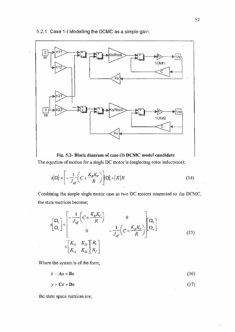
52
5.2.1 Case 1-1 Modelling the DCMC as a simple gain.
Fi2. 5.2- Blocl{ dia2ram of case (D DCMC model candidate
The equation of motion for a single DC motor is (neglecting rotor inductance);
s[aJ + J~ (c+ KsJv) JaJ+[KJR (34)
Combining the simple single motor case as two DC motors connected to the DCMC,
the state matrices become;
o
Where the system is of the form;
X Ax+Bu
y=Cx+Du
the state space matrices are;
(35)
(36)
(37)
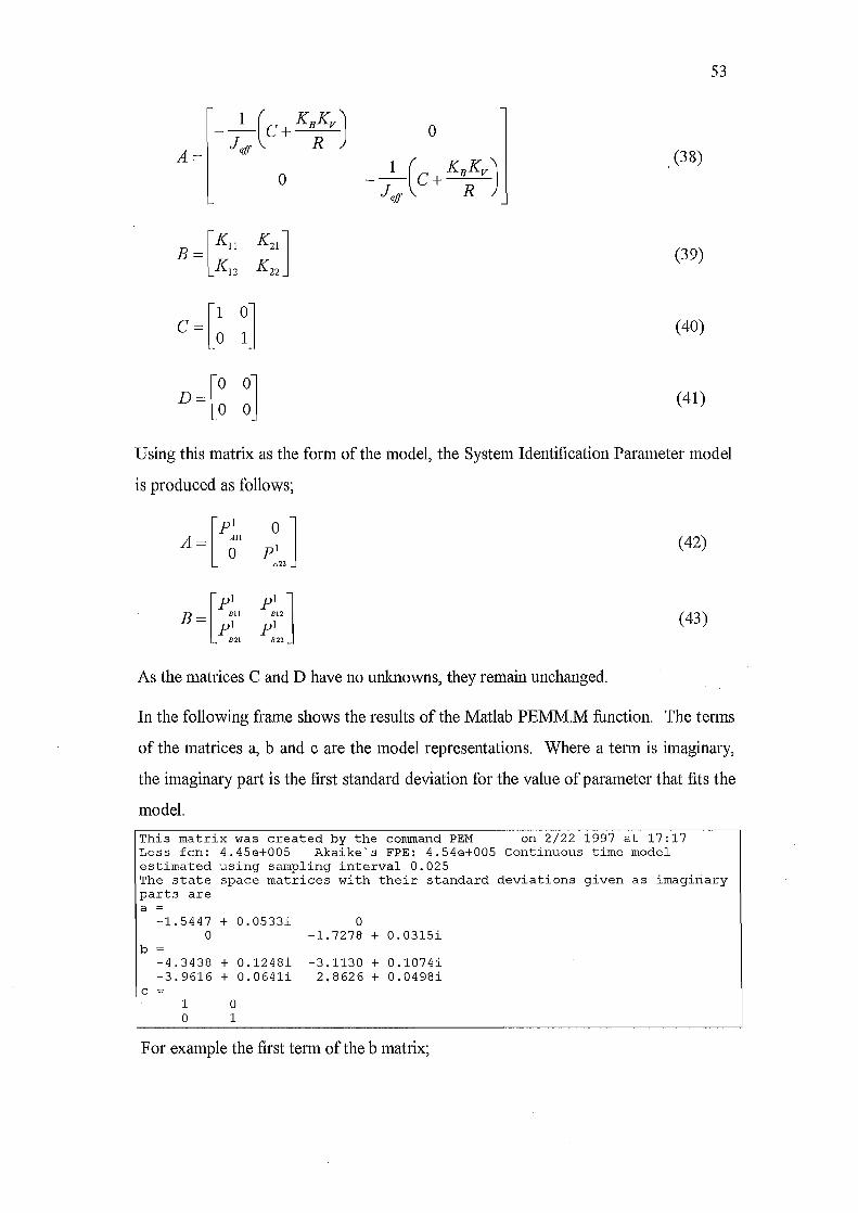
53
o A= . (38)
o
(39)
(40)
(41)
Using this matrix as the form of the model, the System Identification Parameter model
is produced as follows;
[
Pl A = ~11 o ] pl
A22
(42)
[
Pl B = p~l1
D2l
Pl] Dl2
pl E22
(43)
As the matrices C and D have no unknowns, they remain unchanged.
In the following frame shows the results of the Matlab PEMM.M function. The terms
of the matrices a, band c are the model representations. Where a term is imaginary,
the imaginary part is the first standard deviation for the value of parameter that fits the
model.
This matrix was created by the command PEM on 2/22 1997 at 17:17 Loss fen: 4.45e+005 Akaike's FPE: 4.54e+005 continuous time model estimated using sampling interval 0.025 The state space matrices with their standard deviations given as imagiriary parts are a =
-1.5447 + 0.0533i 0 o -1.7278 + 0.0315i
b = -4.3438 + 0.1248i -3.1130 + 0.1074i -3.9616 + 0.0641i 2.8626 + 0.0498i
c = 1 0 o 1
F or example the first term of the b matrix;
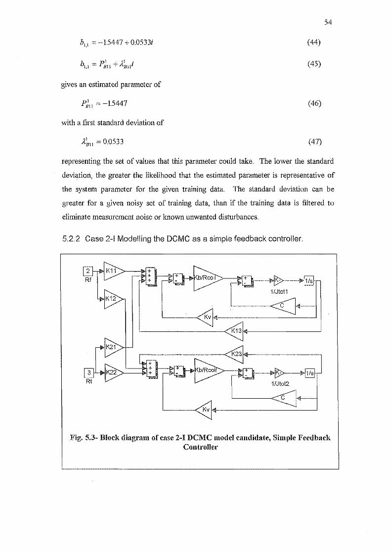
54
bl,l -15447 + 0.0533i (44)
(45)
gives an estimated parameter of
P~11 = -1.5447 (46)
with a first standard deviation of
;t~11 = 0.0533 (47)
representing the set of values that this parameter could take. The lower the standard
deviation, the greater the likelihood that the estimated parameter is representative of
the system parameter for the given training data. The standard deviation can be
greater for a given noisy set of training data, than if the training data is filtered to
eliminate measurement noise or known unwanted disturbances.
5.2.2 Case 2-1 Modelling the DCMC as a simple feedback controller.
~ ~ 1/Jtot1
~----~~~------------------~
~B:>--
~"llI------l
Fig. 5.3- Block diagram of case 2-1 DCMC model candidate, Simple Feedbach: Controller
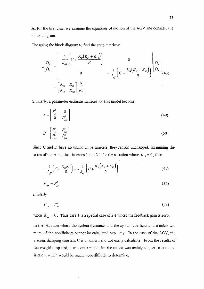
55
As for the first case, we examine the equations of motion of the AGV and consider the
block diagram.
The using the block diagram to fmd the state matrices;
o
Similarly, a parameter estimate matrices for this model become;
[P' A:::: ~1l p~J (49)
[P' P' ] B llll biZ
. p2 p2 b21 bll
(50)
Since C and D have no unknown parameters, they remain unchanged. Examining the
terms of the A matrices in cases 1 and 2-1 for the situation where K]3 0, then
pI = p2 (52) All All
similarly
pI p2 All All
(53)
when K23 =: O. Thus case 1 is a special case of 2-1 where the feedback gain is zero.
In the situation where the system dynamics and the system coefficients are unknown,
many of the coefficients cannot be calculated explicitly. In the case of the AGV, the
viscous damping constant C is unk:nown and not easily calculable. From the results of
the weight drop test, it was determined that the motor was mainly subject to coulomb
friction, which would be much more difficult to determine.
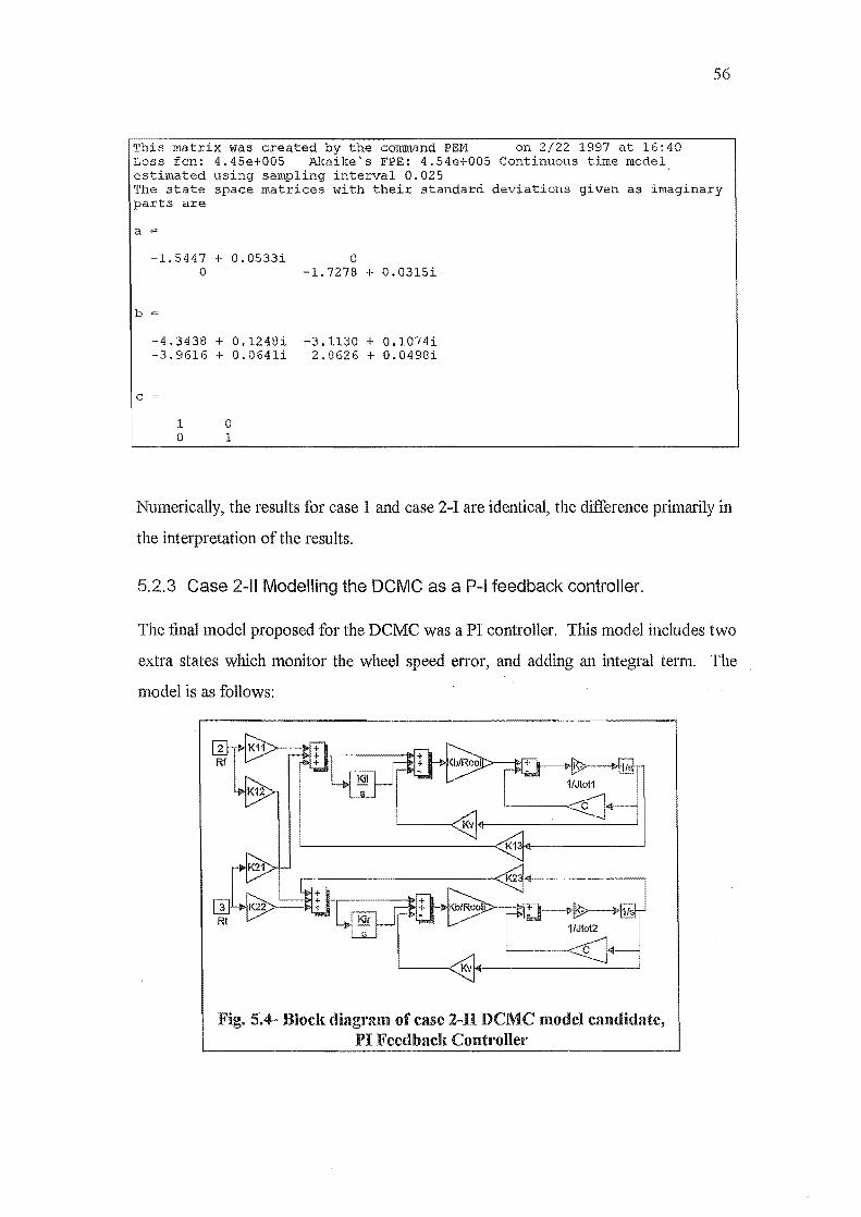
This matrix was created by the command PEM on 2/22 1997 at 16:40 Loss fen: 4.45e+005 Akaike's FPE: 4.54e+005 Continuous time model estimated using sampling interval 0.025
56
The state space matrices with their standard deviations given as imaginary parts are
a =
-1.5447 + 0.0533i 0 o -1.7278 + O.0315i
b
-4,3438 + O.1248i -3,1130 + 0.1074i -3.9616 + O.0641i 2.8626 + O.0498i
c
1 0 o 1
Numerically, the results for case 1 and case 2-1 are identical, the difference primarily in
the interpretation of the results.
5.2.3 Case 2-11 Modelling the DCMC as a P-I feedback controller.
The final model proposed for the DCMC was a PI controller. This model includes two
extra states which monitor the wheel speed error, and adding an integral term. The
model is as follows:
'-----< Kv~-----------'
Fig. 504- Bloclc. diagl'am of case 2-ll DCMC model candidate, PI Feedbacb: Controller
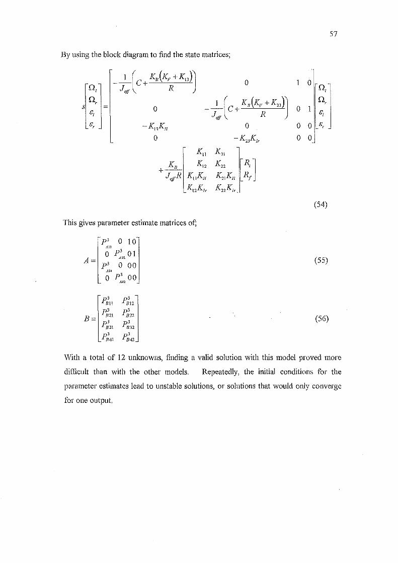
57
By using the block diagram to find the state matrices;
0.1
__ 1 (c + K.(Kv + Kll )]
Jell' R 0 1 0
0.1
nr 1 [ KB(Kv + K,,)] nr s = 0 0 1 81 J C+ R 81
cff
8 y K13KII 0 0 0 8 r
0 -K23Klr 0 0
KU K21
KB K12 K22 [~J +--KI1K]J K21Kll Je.D,R
K12KJr KZ2K1r
(54)
This gives parameter estimate matrices of;
p 3 0 10 All
A= o p 3 01
A22
p 3 0 00 (55)
A31
o p 3 00 .H2
Pill Pi12
B= Pi21 Pi22
Pi31 Pi32 (56)
Pi'll Pi'l2
With a total of 12 unlmowns, finding a valid solution with this model proved more
difficult than with the other models, Repeatedly, the initial conditions for the
parameter estimates lead to unstable solutions, or solutions that would only converge
for one output
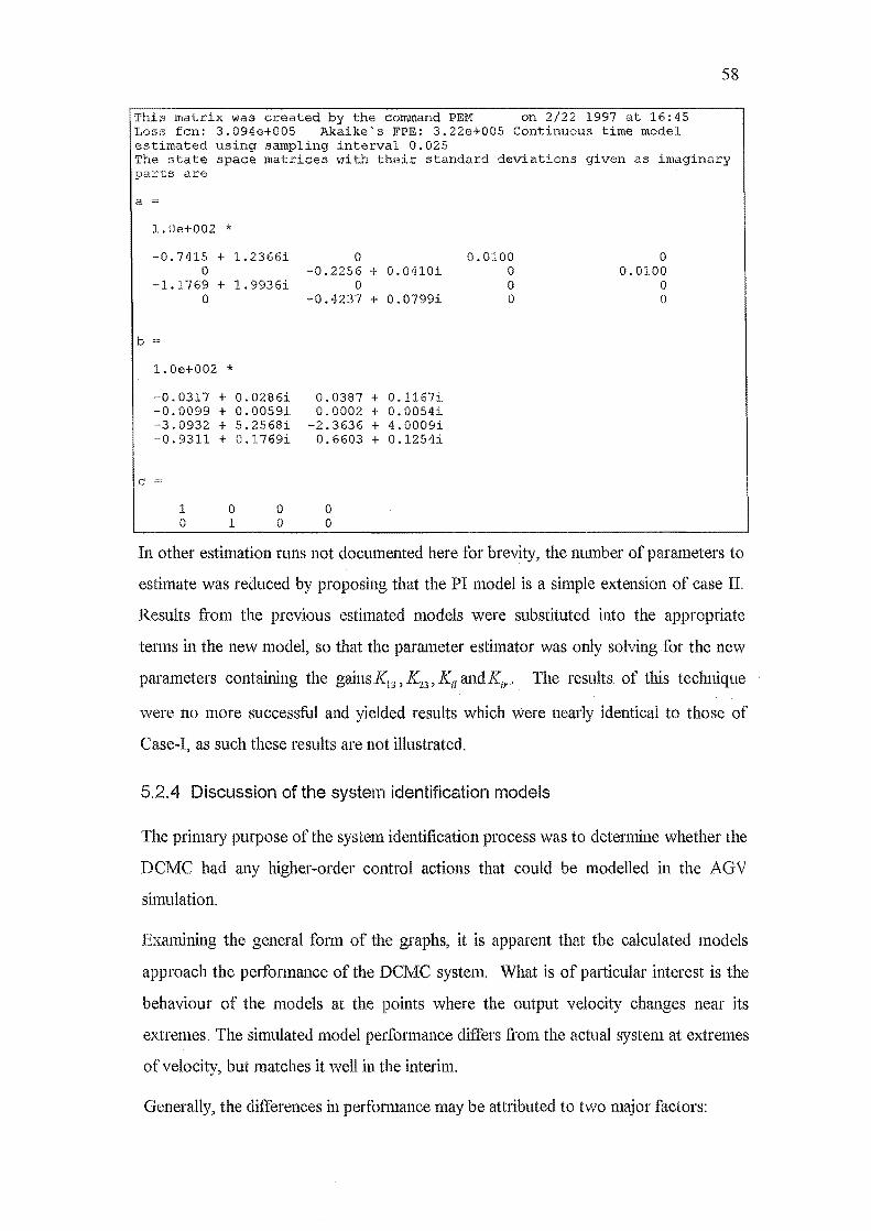
58
This matrix was created by the command PEM on 2/22 1997 at 16:45 Loss fcn: 3.094e+005 Akaike's FPE: 3.22e+005 Continuous time model estimated sampling interval 0.025 The state space matrices with their standard deviations given as imaginary parts are
a
b
1.0e+002 *
-0.7415 + 1.2366i o
-1.1769 + 1.9936i o
1.0e+002 *
-0.0317 + 0.0286i -0.0099 + 0.0059i -3.0932 + 5.2568i -0.9311 + 0.1769i
c =
1 o
o 1
o o
o -0.2256 + 0.0410i
o -0.4237 + 0.0799i
0.0387 + 0.1167i 0.0002 + 0.0054i
-2.3636 + 4.0009i 0.6603 + 0.1254i
o o
0.0100 o o o
o 0.0100
o o
In other estimation runs not documented here for brevity, the number of parameters to
estimate was reduced by proposing that the PI model is a simple extension of case II.
Results from the previous estimated models were substituted into the appropriate
terms in the new model, so that the parameter estimator was only solving for the new
parameters containing the gainsK13 , K23 , KiJ andKir .. The results of this technique
were no more successful and yielded results which were nearly identical to those of
Case-I, as such these results are not illustrated.
5.2.4 Discussion of the system identification models
The primary purpose of the system identification process was to determine whether the
DCMC had any higher-order control actions that could be modelled in the AGV
simulation.
Examining the general form of the graphs, it is apparent that the calculated models
approach the pelformance of the DCMC system. What is of particular interest is the
behaviour of the models at the points where the output velocity changes near its
extremes. The simulated model performance differs from the actual system at extremes
of velocity, but matches it well in the interim.
Generally, the differences in performance may be attributed to two major factors:
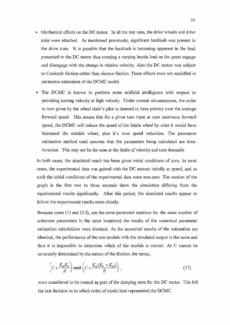
59
& Mechanical effects on the DC motor. In all the test runs, the drive wheels and drive
train were attached. As mentioned previously, significant backlash was present in
the drive train. It is possible that the backlash is becoming apparent in the load
presented to the DC motor thus creating a varying inertia load as the gears engage
and disengage with the change in relative velocity. Also the DC motor was subject
to Coulomb friction rather than viscous friction. These effects were not modelled in
parameter estimation of the DCMC model.
® The DCMC in known to pelioan some artificial intelligence with respect to
providing turtling velocity at high velocity. Under normal circumstances, the order
to turn given by the wheel chair's pilot is deemed to have priority over the average
forward speed. This means that for a given turn input at near maximum forward
speed, the DCMC will reduce the speed of the inside wheel by what it would have
increased the outside wheel, plus it's own speed reduction. The parameter
estimation method used assumes that the parameters being calculated are time
invariant. This may not be the case at the limits of velocity and turn demands.
In both cases, the simulated result has been given initial conditions of zero. In most
cases, the experimental data was gained with the DC motors initially at speed, and as
such the lllitial conditions of the experimental data were non-zero. The section of the
graph in the first two to tlu'ee seconds show the simulation differing from the
experimental results sigcificant1y. After this period, the simulated results appear to
follow the experimental results more closely.
Because cases (1) and (2-I), use the same parameter matrices (ie. the same number of
unknown parameters in the same locations) the results of the numerical parameter
estimation calculations were identical. As the numerical results of the estimation are
identical, the performance of the two models with the sllnulated output is the same and
thus it is impossible to determine which of the models is correct. As C cannot be
accurately determined by the nature of the friction, the terms;
(57)
were considered to be treated as part of the damping term for the DC motor. This left
the last decision as to which order of model best represented the DCMC.
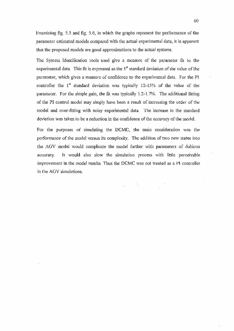
60
Examining fig. 5.5 and fig. 5.6, in which the graphs represent the performance of the
parameter estimated models compared with the actual experimental data, it is apparent
that the proposed models are good approximations to the actual systems.
The System Identification tools used give a measure of the parameter fit to the
experimental data. This fit is expressed as the 1 st standard deviation of the value of the
parameter, which gives a measure of confidence to the experimental data. For the PI
controller the 1 st standard deviation was typically 12-15% of the value of the
parameter. For the simple gain, the fit was typically 1.2-1.7%. The additional fitting
of the PI control model may simply have been a result of increasing the order of the
model and over-fitting with noisy experimental data. The increase in the standard
deviation was taken to be a reduction in the confidence of the accuracy of the model.
For the purposes of simulating the DCMC, the main consideration was the
performance of the model versus its complexity. The addition of two new states into
the AGV model would complicate the model further with parameters of dubious
accuracy. It would also slow the simulation process with little perceivable
improvement in the model results. Thus the DCMC was not treated as a PI controller
in the AGV simulations.
Input #1 100'-1 -----r---,--------,
(i) 50 ~~.
~ C/)
.2 0 '0 ~ o ----a::: -50
::::~_i~~::m ' .. ~tt
·:·::·~·:wu·····tJ·r~H. wv~ 11
Output #1 300~1 ----------~------------.-----------~
'U' 200 c o o Q) (f)
en c co '5 ~ '-" "'0 Q) Q) 0-
r./) -200
-100 1 -300 o 5 10 15 0 5 10 15 Time( seconds) - Experimental Time(seconds) .
. Simulated rw21.dat,with: TRYSS2.M Input #2
1001---,------r----~ ,
! 50 ~t=irtrr:tI .. ~n ... n .. ~JC ........ " () C/)
.2 0 fllll·····----j ~··++---I----~ .~n---I-~-~·-~---~---I-· ---I-~--·-,-·, -•• ,-------.-
'0 ~ o ---~ -50 ---------" ---~~ ---1--' -~ +~ --+~ + -+--+---/---. -~ _L -- ,-, -~,-, .
,
'" HlA) ~ w II+I~ I~ V~
-1 00 L-~ __ __L_ ____ __1__ ___ ---.J
o 5 10 1 Time(seconds)
Output #2 200rl --------~--------~--------~
'U' c o o Q)
~ c co 0 f.-------------.J\: '5 co ''-" "'0 Q) Q) -100 0-
r./)
~OO~I --------~------------------~----------~ o 5 10 15 Time(seconds)
~ .. ~ ~ UII
~ N ~
Q.. ~ S'" ""'3
~ CJ1 CJ1 !Y ~ 0 ~
~ ~
3 <:l Q. (I) -If iooooI
0\ ......
-(]) OJ 0 CI)
~ --0 ~ 0 "-'"
a::
100
50
0
-50
-100 o
- Experimental . Simulated
Input #1
5 10 Time( seconds)
Input #2 100
1 . I ' CD 50 ~,r:1~r~t~hLlt1 .. f~l ..... rr-1jr ro o in
o ~1--.. ··· .. j~··H .. ·I·· .. ~·~n.-.j.~·~-·~ .. ·~··-!--· .. !-~-··-··"··
~ o -......-
C2 -50 1-- ·1++ -~- --~ ... , _ ... -;-~.-.-, .M._
300,
B' 200 c o () (j) en
en c .~ 0 "U CIJ L...
:0 -100 (j) (j) 0.. (f) -200
-300 15 0
rw21.dat,with: TRYSS3.M
r.
200
.....--. "U
§ 100 () (j) en en ffi 0 :0
CIJ L...
15' (1) (1) -100 0.. (f)
Output #1
5 10 15 Time( seconds)
Output #2
L,. l.wJy ~ ~ '!+l~ I ~ V\o-J
-100 o 5 10 15 Time( seconds)
_2001----------L---------~--------~ o 5 10 15
Time( seconds)
~ ... rKI
01 e.. ~ N ..... Q., ~ -::Jl ... -:::r .. >-3
~ 00 00 .~
~ 0
~ ('1
S 0 Q., ('!> -N I
1=1
0\ N
6. RESULTS AND CONI
AND LABORATORY
OF SIMULATIONS
6.1 INITIAL CONDITIONS FORAGV LA BORA TOR V TESTING
63
The AGV has a limited sensor range « 150 mm), and the laboratory space available to
perform the tests was limited. Hence, at the start of each experimentallUn, the AGV
was manoeuvred parallel to the guide wire with the sensor pair offset approximately
120mm from the guide wire. These initial conditions were effectively a step input in
displacement from the guide wire combined with a step input in forward velocity after
starting the control algorithm. The offset from the guide wire was chosen such that
the AGV would be within the sensor range, and would not have to exhibit any
'searching' behaviour in order to find the guide wire. Such evolutionary behaviour
would be difficult if not impossible to accurately model in the simulation.
RESULTS OF SIMULATIONS
Generally, the more complex of the Matlab simulations show good correlation with the
experimental results. Unfortunately, the greater the complexity of the model, the
greater the time taken for the calculations.
In order to make a meaningful comparison between the simulation and the
experimental results, initial conditions for the simulations were used that were similar
to those used in the laboratory experiments.
6.2.1 Simple Linear Second Order Model
This model has the AGV on a flat plane free to roam in 2D. With the transformation to
2D, the minimal AGV becomes considerably more difficult to control. The AGV is
directly provided with feedback of the known sensor location.
The performance of these simulations is not representative of the existing AGV
system, but it does provide an indication of the performance of an AGV system with
complete knowledge of the sensor location.
64
Figs. 6.1 and 6.2 show the performance of the AGV model with increasing
proportional gain. As the gain is increased the AGV follow the guide wire (or desired
path as is the case in this model) with a reduced tracking error. The model is damped
and when the DC motors saturate, the model pelformance moves asymptotically to a
minimal error with increasing proportional gain. Brief checks with gains of 2 orders of
magnitude greater that the largest gain used on the AGV experimental runs confirm
this. This asymptotic trend is shown clearly in fig. 6.2.
A numerical approximation to the non-linear system of equations describing this model
was calculated for the given operating points using simple derivative approximation
tools. These tools perturb the inputs to the model, and use the changes in the outputs
to calculate an approximation to the state space matrices. Subsequently, these state
space approximations were examined for observability and controllability of the model.
From the analysis, this model of the AGV proved to have all states controllable, but
only two measured states with the given sensor equipment. For full feedback control
of these unobservable states, more feedback information would be necessaly. This
feedback could be gathered either by adding more sensors, or by adding an observer
(or Kalman Filter) to the control system to estimate the unlmown states.
6.2.2 Complete !\Jon-Linear Model
Figs 6.3 and 6.4 show the same characteristics as the simple linear model. The
performance of the AGV simulation becomes asymptotically closer to a minimum error
as the control effort is increased. This model includes the operation of the sensors as
they were implemented on the actual AGY.
The plots vary from the simple linear model accordingly. When the AGV is further
fl:om the guide wire, the sensor strength is low and the model turns slowly toward the
desired path. As the AGV turns to the guide wire, the sensor models show increased
signal strength and the position error (as it simply the difference between the signal
levels at the sensors) increases briefly until the sensors are positioned either side of the
guide wire. Where the simulated AGV is nearer the desired path, the performance of
the linear model and the non-linear sensor model are more similar.
65
6.2.3 Complete Complex Second Order model with Backlash
Fig. 6.5 demonstrates the performance of the model of the AGV complete with
bacldash between the gear train and the wheels. For these simulations, the bacldash of
the model was set to a value similar to that of the actual AGY. What is most distinct
about these paths is the introduction of limit cycles that manifest themselves as
oscillations in the AGV s displacement from the desired path.
With the increasing proportional gain, two features of the traces are noteworthy:
1) The AGV model attempts to reach the same asymptotic path as simpler models
2) The amplitude of the limit cycles increases, as the AGV model is given greater
energy between the bacldash cycles.
6.3 COMPARISON OF LAB RESULTS AND SIMULATIONS
The laboratory results and the simulations show similarities in many features of their
performance. The results of the simulations are considered here in the light of the
results of the experiments, and the possible reasons for the differences are discussed.
6.3.1 Comparison of the Backlash Model with the Experimental results
The measured AGV responses are compared with the simulated responses figs 6.6,6.7
and 6.8. The experimental results obtained show excellent agreement with the
simulations over a 21: 1 change in the system gain. However, examining the results of
the lab experiments, it is immediately apparent from Run#3 (fig. 6.8) that assumption
of no-slip is invalid at high feedback gain. Although its not obvious from the graph,
the micro controller was observed to be saturating the DC motors and over driving the
AGV well into backlash. The AGV was being driven so hard that the differentials in
left and right wheel speed would cause an exaggerated rotation that the control system
would attempt to negate by driving the AGV in the opposite direction.
The bacldash in the gear train has the effect of aggravating the traction conditions at
the wheels. As soon as the gear train began to engage after the DC motor has been
freewheeling, the wheels are accelerated abruptly, lose traction and spin. The spinning
wheels have less tractive effort on the ground. Thus the AGV increases speed to
accommodate for the increased error at the sensors, and establishes a limit cycle
66
oscillating between full speed wheel slip in either direction as the sensor oscillates
across the guide wire.
The onset of the limit cycling through the AGV backlash region is aggravated by
increasing the proportional gain. At lower proportional gains, (and thus lower control
effort), the backlash model simulates the AGV with better accuracy. Fig. 6.9 shows a
comparison of the experimental run at low proportional gain with two simulations at
similar gain values. Each of the bacldash simulations tracks the experimental results
well near the beginning of the run, but an error is apparent in the middle phase of the
run.
6.3.2 Potential Sources of Model Inaccuracy
In the simple models where the bacldash and slip are not included, the higher gain
models will apply more torque to the AGV wheels for a given error. In these models
the torque is assumed to be transmitted to the AGV chassis via the tractive effort of
the wheels. In reality this has proven to be incorrect as the wheels break-away from
the no-slip condition and introduce a new state of dynamics to the system in the form
of relative velocities and interaction between the wheels, the AGV chassis, and the
ground. As such, the no-slip condition is a major source of inaccuracy in the models,
as will be discussed.
Another source of inaccuracy is the assumption that the majority of the friction in the
system is viscous. This was a necessary assumption for the sake of classical analysis,
but with the availability of powerful numerical tools such as Simulink, it may be
possible to include other forms of friction in the models, although this was not
attempted. Apart from the results of the Falling Weight Test to determine the
properties of the DC motors, there was no immediate measurable evidence of 'stiction'
in the AGV system.
6.3.3 Potential Sources of Experimental Error
The primary source of experimental error is in the operation of measuring the points
laid down on the paper, and in the physical layout of the experiment itself.
The paper was taped to the floor over the guide wire, and despite all efforts to the
contrary, the guide wire was known to be linear only to within ±3nun. This source of
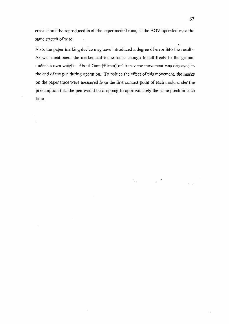
67
error should be reproduced in all the experimental runs, as the AGV operated over the
same stretch of wire.
Also, the paper marldng device may have introduced a degree of error into the results.
As was mentioned, the marker had to be loose enough to fall freely to the ground
under its own weight. About 2mm (±l1nm) of transverse movement was observed in
the end of the pen during operation. To reduce the effect of this movement, the marks
on the paper trace were measured from the first contact point of each mark, under the
presumption that the pen would be dropping to approximately the same position each
time.
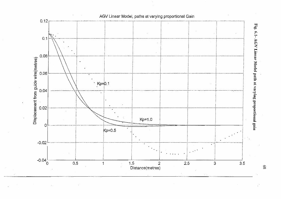
c 'ro <.9 ro c o t o a.. e a.. O
l c '~
ro >
...... ro (/) .c
...... ro a.. Q
) '"0 o :2 I
ro Q
) c ::J >
<.9 «
Fig. 6.1-A
GV
Linea.' M
odel path at varying proportional gain
f ~--~ ...... ~ ---~ ~ .. --r --.. ~-~-----
~-. ---r~"""'"" --.. -_ .... ----f-----........ -_ ...... ---i,.,." .... --------...... -: -.... -"' .. --...... --...... -: ........ --........ --...... "'": ---..... -~ ~ ..... ,,; .... !
: iii
: !
:
: :
! i
! i
:
! 1
i !
I'!
l I
* I
I f
I I
i ~
~ j i!
! :
: :
1 ::
: :
: i
: ::
: I
• j
I I
I ..
~ 4
, •
I I
I I
I •
I i
I I
I I
, f
I I.
, I
I I
I 't",
,······· .. ····· .. ·~· .......... · .. ···f·· .... ····-···· .. f ...... • ........ ··,···· .... • .... • .. ·1······ .... · .. · .. · ................. , .............. . 1
: :
! !:
r t
• I
I I
I t
1 iii
! i
i 1
i !
! !
i i
I ,
I i
I I
I
: l
! j
j I
i '
I t
I I
I ,
l ................ .l ................. L ................ L
................ 1 ................ .1 .................................. J .............. . :
: :
: ::
: i
i l
! Ii!
f !
I !
I j
I
! !
! i i!
i I
f I
i I
I ,
I I
j I
I I
I I
I I
I I,
,
: :
: : ::
: '
• I
I I.
I I
, •
f I
* I
I •
I I j,
• I
I I
I I
I I
' I
I I 'l
I I
I j
I I
I I
' I
I t I.
I '
I I
I I.
I
~.,. ...... "
.. -
-...... _
.. _
-.. ~~b
----
.... -
_ .. ~ ------~
.. ---
.......................... ~
------
.. ~
'" ................. t .. ~ .................... -----i ............... ---............ ~ i .. -...................... "' .. i.w _ .... ~ __ .. ",. ...... ..
I •
I j
I t
I I
I I
I •
I t
j I
I I
I •
I •
t ,
I I
I I
I f
I I
I t
I •
I ,
I I
I I
I j
I ,
f I
I I
, f
I I
• I
: !
: :
: :
0:
: •
I t
I I
, •
• I
I ,
t f
, t
t
: :
: :
: I
-r-:
i :
: :
: ~
: II:
: • If.
I I
'a
..
' f
: :
: :
! !~;
1 !
' I
j ,
I ...x
...
, ,
If,
I •
I ,
, '
• I
I •
I I
I t
f j
f ;
I I
I I
I ,
I I
, f
I I
I j
t I
f I
I •
• I
, ,
, I
I I
, I
, I
• ,
, ~-
---~""*,,"ft_""""" _~ .......... _
__
__
__
__
__
".~ ............ "'M ............ ,. .... ~ .. _
__
__
_ .. ____ ........ "! ........ " .. ,, ....... ______ ! _____ ...... _ .. _........
.. ~ ___ .... __ .. __ .......... ~ .. __ .. " .. _ ...... _ ... _ ..
' I
• I
I ,
I.,
• I
I I
I t
I I
I I
I t
I •
I I
I I
• i
I •
I I
' ft.
I •
I I
t I
I •
I I
I ,
t ,
I •
I I
, f
' •
t I
I ,
j I
: :
: ,
: :
. : :
I I
I ~
I I
I I
• I
, t
I I
I I
! I
I I
t f
I I
f I
, !
I f
I •
I I
I I
I I"
• I
, I
" I
: :
: :
: :
LO
:
" I
I •
f r
I
: :
: :
: :.
0:
i :
! 1
i ' :
jill
I I
, I
-r-I
f 1
.0
..
I '
j I
I.
I I
; ~
,
~ ~ ~ --~~~ ~ --~~-~~ .. ~~ -~~ -~ .... -------.. '"'-~ ---~ ----"" ...... -.... -~--------.011 " ......... ~ ~ .... --.... ---: -.. __ ..... i .--.. -...... ~ ~ .. --~ ---
.... _--_ .. _--~"~,, ~ .. '" --.. ---..... I
I j
I I
• I
,
f •
I '~
I ,
I I
I •
I ,
I I
I I
~ I It.
• I
, •
• I
, I If,
I I
I •
I I
I I
i •
I I
• ,
, I
I I
, I
I I
I t
f I
I If.
I j
I I
I I
I ,
t I
• I
I I
I It.
• I
j I
I I
I •
t I
• I
I I
j t
t I
I I
I I
t f
•
: :
: t •
~ :
j ,
I f
~ t
I f
I I
, ••
" '
, I 'l
I I
! j
, '"
I I
I * It.
• I
I * If.
f j
I "
, I
f I
I I
f I
f I
j I
I , Iff
I I
I f
I f
I I
I I
, I
I I
I •
~ --~ ...... -~~ -~. _. ~.t ~ ... " ........ _.~.~ .. w
.. ~ .
.............. _
.. _ ~ ..... ~ •
••• ~~_._ .
. ~.
.. .......... _
_ ._
...... ~_ .. _
,. ................... ,.,.~
_" ......... _
__
__
.. ,," ~
.. ~ .... _
.... ",. ..... _
..... ..
, f
I I
I.
I I
, I
I J
f f
' I
I I
It;
I t
I I
I.,
j ,
! f
f f
, It,
,.
I I 'l
I I
I I I.
I,
I I 'l
i I
I I I.
• I
I f
" •
I I
I •
t I
I I
J •
I I,
I •
I I
I I
• f
, I
j •
t I
fl.
' I
j I
I '
• •
I I
' I
I I
, '
j I
I I
t •
t I
I •
f •
I I
I ,
f I
I
• ,
, *
' f
I I
' I
, ,
00
o
~
~
~
00
0
a o
( S9JlaW)SJ1M
ap!nB W
OJj luaW
9081dslO
N
LO
r-
LO
a 68
.--. (/) (}) I-
...... Q
)
E
.......... Q
) (J
c ro
...... (/)
is
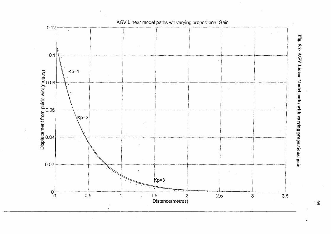
c 'ro (9
ro c o :e o a. e a. 0
)
c .~
~ ...... .~
(J) .c
m
a. ill "0
o E
I-
eo (I) c :.:i >
(9
«
Fig. 6.2~ A
GV
Linear M
odel paths with varying Pl'opO
l'tional gain
~ .. ~
-" ....... "'"" .. ~
--""" ..........
-~
-.. -
-" .. "
...... "" .................. w
... _
.......... A
................ ,. ........................... _
_ ... _
"' .
.......................... "
.............. "
.. _
__
.. ~ .
.......... ,. _
_ ........... "
__
.............. ..
I It;
t i
I It.
t j
• I
I I
I I
I I
• I
, •
! 1
i i
! ~
• ,
I ,
I I
: :
: :
: :
: :
: :
: :
! !
i !
! I
iii iii
I .. ········ .. ·· ········ .. t· .. ···· ................ t··· .................... I·········· .. · .......... j .......... , ............ )"" ............ -..... . ,
I •
I j
I It.
t I
, I
t I
I I
I I
• •
• I
j
• I
I iii
: :
: :
: i
' 1
t •
j I
i i
! !
! !
I I
I I
I t
I I
l •
I I
I •
• t
I I
: :
; :
: :
I ,
I I
, I
~ --.... -.. ---.............. -.. -"'---~ -_ .......... -_ .. ----.... " .. ~ .... --~ .... " ....... ""--,.",--,,, --........ _ .. i --.................... --_ .. -............ i-.......... -...... _-...... ,. .............. ~-.. -----.......... ~ .......... --,. l
l !
l i
i '
I I
I I
I
: :
: :
: :
1 ,
, I
I I
~ 1
! i
j I
l I
I •
I t
I I
I I
I I
: :
! :
I :
I I
t I
I 1
j • It.
I I
• I
I I
I If.
I I
I
: :
: !
: :
• ,
I t
I I
r······· .. · ... -....... ··r············ .......... ·t··········· ............ j ....................... j'" .................... j' ................... . I
I I
• I
I I
I Itt
I
: :
1 I
: :
: :
: :
: :
: ~
: :
: ~
: ~
: 1
: ~
I I
f I
I ,
I •
t I
I I
I I
I I
I i
~ i
~ !
~ i
If,
I •
I C
f) :
! :
! :
! II
: :
: :
: :
Q.
t~ ..... ~ ~ .. ~ ~ .. -.... --.. ~ ..... --~ .. "' .. ---........ ~-............. ~,. ~~t ................ ,,~ ................. ~ .... -~ ~ ........ ", .. ~ .............. ,.. .. _ .... " .. ~ ... : .......... ,. " .................. ___ ~ .. _ .. 1 ....................... ~ "' .. ...
I •
I I
• I
: !
: I
: :
I •
j I
I I
I I
• t
I I
I I
; I
• I
I I
I I
• I
: :
: !
: :
: :
: :
: :
I ,
t I
I I
I I
I 1
I I
: :
: :
: :
: !
: :
: :
I I
I I
t I
I I
I I
i I
• t
I I
• I
: :
I :
: :
• I
I I
i I
: 1
t :
: :
t •
1 I
I I
I I
I I
I t
~ .. -
............ -
.......... ¥
-...... -
...... ~
.......................... -_
.... '"
..... ,. .. ,,~ .
...... _
_ ........
_ .............. _
_ ......... t ........ -.......... ~ .............. '" ,. ...... t" .... ,. .. -.. -.... " .... ----'"'----.. i .......... -... ..
f t
I I
I I
I I
I I
I f
I I
I I
t I
I I
I tit
: :
: 1
I :
I I
I I
, I
I I
I I
• I
I t
I I
I I
t I
I !
t •
I j
, t
I I
j i
i t
~ •
I::,':: 'I,:: 'I,:: ':,
'I::, •
i ! iii .................. , ~i:: ..
.................. .
;.--........ " .. -.. ,.,. .............. " ...... ~,. .... --...... "' .. "'~ ............ "' ........ :. .... -.. -----.. -.......... -...... -~ .. ~ ........ -............... -" .. -........... ~..... -
---
-'
I •
• N
I
: i
! !
II ,
: :
: :
.Q..
I
1 i..-!
! ~. 1::::
I l,~
i :
! !
~!'
! .'
<Xl o
"¢
o
o 0
d (saJlaw
)aJ!M ap!n5 W
OJllU
aWaO
l3ldslO
l()
N
l()
69
-- (j) Q)
I-
m
E
'-"'
(I) u c eo
1?i o
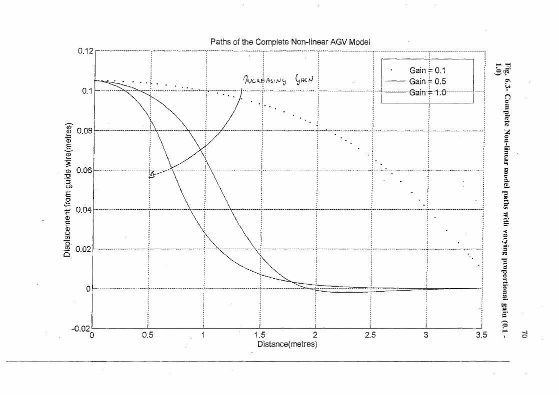
()) -0
o :2:
§ L-
eu ())
.5
I § :;::: 2 Q
)
0..
E
o o Q
)
:5 '0 (f)
:5 eu n..
70
Fig. 6.3-
Com
plete Non-linear m
odel paths with varying proportional gain (0'.1
1.0)
... ~ ~ ~ ............... _
__
,. ........ _
M _
__
__
_ ............ ~ _
__
__
.................. _
__
~""""""""'" _
_ .
. '"
_
_ '"
............ "
.. ~ .......... "
...... ,.,. _
_ ............ _
.. _
.. _
............ _
.... _
_ "_""_""""~"''''''''''''' _
_ .. _
" .......... .
• I
! I
I I
I
: :
: :
: ;
I I
i If.
I I
I I
t I
I I
I t
I
: :
: :
: : .'
I ,
I j
I I
I ;
1 !
1 r
I I It.
, I
I I
• •
I t
I I
I I
I J
f I
I I
I I
I I
I •
I
~ -v
-l.(')¢:l.'.
: i
: :
t I
I I
I
: 0
0;.-
: :
I :
~ ....... II····~~· .. -h ..... · .... ···· .. ··.l .................... ~ ................... i .................... l................... . ............... . :
c c:
i:: :
i :
: i
'00 'ffi
.~ i
! !
1 :
(!Jt'J
(t!) :
: !
: I
I I
I I
I
i I il iii
i I
I I
I I
, I
I I
I I
I I
, I
I I
I
~ !
! : •
: i
: :
: .:
~ :
: I
: •
: :
: j
'I
I I
I 'I
1 I
, I
I I
I I
i'"' --.... " ......... ----'" " .. '" -1-"""" .. ---.. ,,~ .. --.......... t .......... _ .. -............ _-...... -r --
-~ .. ---.... -_ ........ -_ .. ~---.. -_ ............ __ .... -...... t-_ .......... --...... --",,~--.. ~ .. ___
w _
_ ............ _
_
: :
: :
: :
1 i
1 i
! !
I *
t •
I I
I t
I I
I I
I :
: :
: :
I I
I I
I I
I I
I I
I I
I I
I I
I •
: :
: :
: :
t I
I I
I I
' I
I.
I I
, t Ii.
I I
I I
• I
I I
I I
• I
• I
I I
t I
I f
• I
-. J
• I
I I
I I
I •
I I
I I
, I
I I
I 1
I •
~~ .. " ......... ---.. ", ... ~~~ ~ .. ., .. ~"-""""" ~ .. -.... ---.-.. J-~~ .. ----~ .... ---........ --:-. .. _-----.. -... _ .. --"''' --i" -.. -" .. ---_ .. ---" .... --"'.-~ .. -_ .... ----______ .. .. .~ ...... ~ ~""""" __ .. "
I I
I ,
t j
! ~:
! ;
: ~
l I
I *
I I
t .....,J
I I
I •
•
: Q
!
: i
: :
: c;..J:>
: :
: :
: I
I j It.
I I
, J
I I
I I
i I
I I
: :
: :
~ :
: ~:
: !
: :
I •
, I
I I
: :5
1 :
I :
: t
, I
I I
I I
\J)
I I
• I
I
1 d
:::!
: :
! r ........... ----.. -.. -
~ .. ,,-1----...... -.... -.. -....... -_ .. ,,: ...... -.... --... ~ .. --...... ~~-r-.... ~ .................. -.. "' ... '"1-........ ---_ ...... -----.... ~ r""
• 1
-I
, •
, •
1 I
• ,
: J
: :
: :
: :
:? :'
-:
: :
: :
" :
! :
'1 :
1 I.
I I
I I
I I
I I
• t
• I
I '.,
I lit
! I
t 'I
f t
I I
• •
I • fIt
t I
I t
I I
; I
1 I
'I
I I
' ,
: : -
: :
I
· .
,
· · · , , , , , , , ,
...... t········ ........ . · · , , · · , , , , , , , ,
[···· .. ··········· .. i····· .. · .... ········;-······ ,
, ·······;·· .... · .. ··········T········ .. ·······
: -:
I
I I
1 .'1
1 .
1 [--· .... · .. _-_ .... · .. · ...... "1 .. -:
' i I [
, , .
----'f .......... --....... _"'~ ........... ,. ..... _
, ,
; :
: :
, ,
: :
, ,
, ,
, .
: :
: :
. ,
~ :
, ,
! !
, ,
ro o
<D
o ·········r······ ···r······ T····· j
! i
1 :
:
! !
I ,
, ,
'" o o
00
0
0 (S
9Jl9W)9J!M
9P
!n6
WO
JJ lU9W
9081dSlG
1.O
N
1.O o o
'" o c?
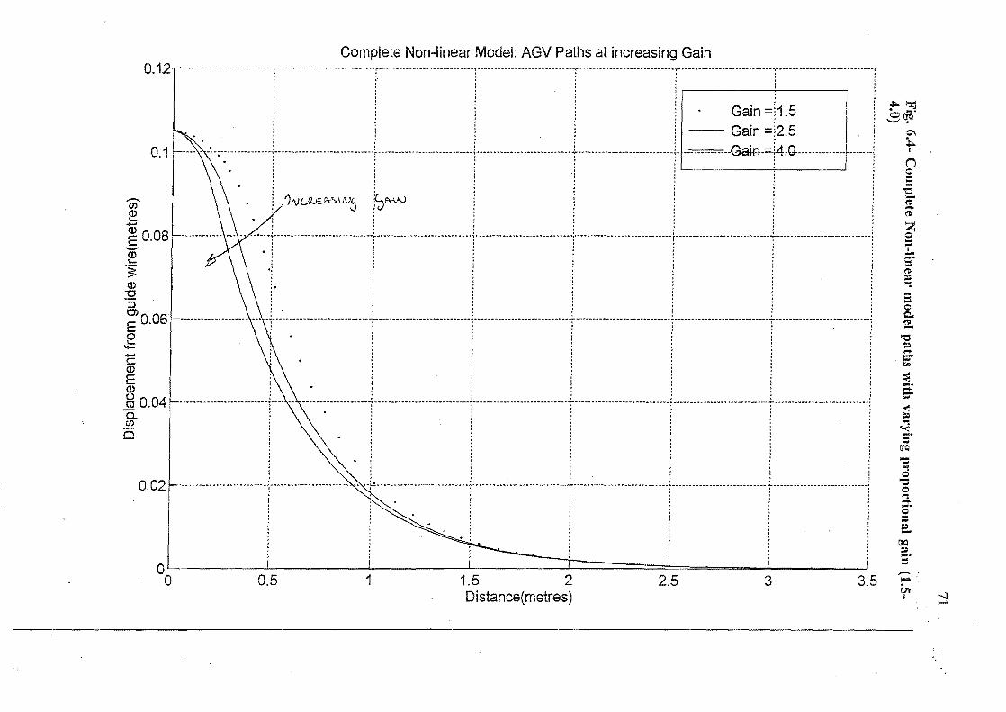
'-ro Q
)
.£
"I
C
a Z
Q)
1i) a. E
a ()
71
Fig. 6.4-
Com
plete Non-lineal' m
odel patbs with
varying proportional gain (1.5-4.0)
~ ~
~ o
0 c:i
(saJlaW)aJ!M
ap!n5 WOJJ lU9W9~elds!a
,... c:i
N
o c:i
o o
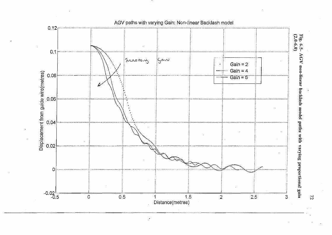
(j) "0
o E
..c (/)
cu U
cu 0
0
I-
cu (]) C
I C
o Z
c: 'ro (!) Q
) c '~
cu >
(/)
~ a.. >
(!) «
72
Fig. 6.5-
AG
V non-linear bacldash m
odel path
s with varying proportional gain
(2.0-6.0) ,~----~ .... ,. .... ~ .............. ~ ~ .. ~ ..... ~---
.... _ .. ~ .... ~ .... i ""_"M
.. '" ---
M M
............ --r-"" ........ -------_ .... -.. ,"' .. ------.................. _--j-
""""" _ .... "
" --
...... ~~--t..
. _ .......... ~ ...... __ .. ,
• I
• I
I •
I !
I t
I I
I '
I I
, I
~ I
~ I
• ,
I I
• I
I ,
t I
, I
• I
f I
I I
I '
1ft
• I
I I
I •
I f
I I
• 1
t ,
f I
I '
I j-
I I
I I
I I
t I
I I
• \
I ,
I ,
I ,
I I
I I
; I
,
: :
: :
: :
: If,
I ,
t •
I I
I I
, I
• f
I I
, I
• •
I I
I ,
• I
I 1
! ,
I •
• •
: :
: :
: :
to :
iii
1 i
i \1.
~------.............. -_ .. -"' .. {M .~.. --------.......... " .. ~---------.... _ .. -.... ___ : .. ____ "' .... "' ...... ~"_""" _ .. i _ ... _____ ~ .. ~ .. " ...... _ "' ....... ~ ........ ___ ~_ .. __ ~ ____ .... _::\" , .................. __ .... .,
i !
• :
: :
: i :
: t
: I
! : 1
i !
. :
: :
1/ :
: ('\J~~
i :
: ..t"
: :
II II
~ II :
: !
... :
: i.£
; .£: :e
: ~
: i
~ j
co cu till
i ~
i (
: i
(!)(!):t!) l
: i
\ •
I I
I I
I
f· .........+ ....... :.J I: "I···· ....... +..........j ........... -1-........... ···l······ .. .
: : Ii:
: ;
I I
I.!"
I I
I,
I •••
I I
I I
j •
I
• I
.."
· I
I..,
• I
I It,
I,
t I'
• I
I I
Itt
I i
I I.
I I
::
I:::
t I
I.
I I
I I
I I
I I
I i
I.
I I
I I
I I
I I
I I
I I
I I
j I
I I
, I
l!
i!:
I ! :
: I
: :
: I :
II. ~ -~ .................. --~-...... {~"',. ........ _ .. " ...... -
-.-. ~ ..... --", -
... " --
.... "' .... -----~--.. -
-.......... ,. .... ,.. .......... i----"" _ .. -.......... ,,-----t .. "' .... ___ .... __ ....
.. -I~ '" _:_~_.,. .. -. .... _____ ~ ...... ~ :
: :
: :
: /
: I
I 1
I •
, !
J I
, I
t I
!
: :
: :
: :
; t
I I
I I
I !
: :
: :
: i
: '
• t
I I
I I
t I
I I
I I
,
: :
! !
1 !
: ~
f !
! !
i !
: ~?:
: :
: :
l f -':
: !
: i
: :
d: l
! :
:,
: :
: JV
:
~ :
; .," :
1"'--",. ........ ,. .. ,. .. --.. __ .... "0----___ ,.,.,. .............. _. _,." .. __ ............ "",. .... _____ ,.. ... __ .. __ ............ "'''',. ~"" ; _____ .................... .............. .... .. ........ ___ ~ .. _ .... _.-_",,~ ,._ .. _ .... "' ........ __ ..
: :
: :
: ,-:
: :
: !
: :
,.' I
:
: :
: :
: l
: I
• I
I I
~
I
~ i P
!
! 1-
•.•.•. i
t i.):
: I
,,-:
t i
~
i ;
! •••••
i I
I •
It..
I
! :
w:
: . ~.. .
: I
,d
It.
" j
: : J:
:. .
: :
: :
2.:
~. . . .. 1
:
: :
C'"
~ .... :
: :
: ~~ ... --..... ~ ~ _. --_ .... ---1--~~~ ............... -" .. " .... -t -_ .. -..... ".~.~ .-~---.. -~ -------.
" .. -1----..... --.......... '" .... "' .. ~ t .... _-.. --....... ~ ~ ~ .. " .. _ .... _;-"''''' ~ ~ ~ ............ " ... __ :
: :
. ":
: :
: :
: .:. ..
: :
: :
: ::
: 1
: It.
I I
I I
l f
I I
I I
I *
I,.
I I
• I
• I
I I
I ,
fl.
I ,
! : .,.
::!
: 1··
:::
i .,··"l
:::
: /
t:
i *
• •
I t
I ,
I
~ :
: :
~ ................. _ .. ".... ----..:-~-----... " .... -"~""" --~-------." ... " ,,--.... ---~--.. --" .. ---.. _ .. _,.., .... " ~---.. ----.... _ .. _---...... ~~ .. ~ .. ~~~. -----.. -.... ,. .. ~ ~:~ -. -'" ~-.. ~ ------.... .,
I I
I i
j I
1 I
I I
I I
I ,
I I
I ,
j I
t I
I I
i I
t I
: :
: :
: :
: '
I I
I I
, I
I I
I I t'l
t I
I I-
I I
• ~
, I
j t
, I
I ,
I J
t I
• I
I •
I I
1 I
! ,
• I
• *
• I
I ,
.. t
I •
I I
• f
I t
1ft
I I
I •
1 I
• t
* If,
I I
j •
f I
I I
I t
I I
I I
.! :
: :
: :
I I
I I
I I
! I
I •
I ,
t •
I I
• I
' Itt
'. I
o co o
<D o
~
00
0
0 (S9Jl9W
)9J!M 9P
!n5 WOJJ lU
9W90elds!O
o
LO
N
LO o o LO
N
O
0'
o ,
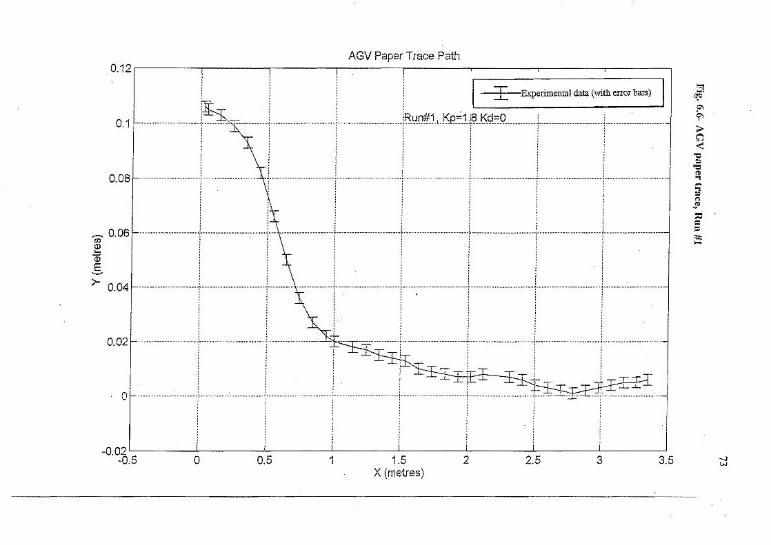
-(f) ~
1i5 E ->-
AGV Paper Trace Path 0.12.1 --------.--------.--------.-------~-------,~------~------~--------,
0.1
0.08
0.06
0.04
0.02
o
· · · ----------------------j"------------------------r--· . · . · . , . · , , , · , · , · , · . · . , ,
I E:h.-perimental data (with error bars)
iRun#1. !:<j)~.1'i_Kg=Q
.
. --------.. --.. ----.. -- .. -----
------........... r-............. ------· · ·
---........ _--"-- .. --- --_ ... --- ...
· ·
---"'''' .. ---~------,. -_ .. ----· · · ~
1 1.5 -0·~t:5 a 0.5 X (metres) 2 2.5 3 3.5
~ ~.
Q\
Q., I
> ~
"'0 ~
"'0 I't> ., '"'" ;;i ~ s:-~ = ... -::j:I:; >-"
-.-J w
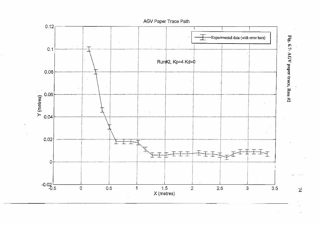
-CJ)
~ 1» E -->-
AGV Paper Trace Path 0.12'1 -------.--------,--------,--------,-------,--------,--------.-------,
I Experimental data (with error bars)
'; . • I • ~ ----------------------f---± .. ------------ .. ---1---------- .. "'-----_ .. -- .... --1---- .. -- -- -- -- ---............. _ .... f ............... -- --_ .. _ .. -----.. -- .. -r ..... ""-_ .... -.. --------.. ------1-------- .. ---... -.----.. ----- ---.. -_ ...... ~-------------0.1
I • • • , ; , • I t • f , j I I • • • ~
I I "
1 1 Run#2, Kp=4 Kd=6 ! · . · . · . · . · . 0.08 · . · . .. -..... --......................... --.... ---- -_ .. ---.... -.. ..
; . · . · . · . · . · . · . · . · . · . , . , . · . · . · . · . · . · , 0.06 · . ····_·,····················-r
· , . ............... 1" ... "' .......... ____ .. ____________ -'0-_.
, . , . 0.04 , . · , · . ................. ""' ......................... _-----------.... -, . , . , . 1---+--+1 -3 0.02 , , , . , . , . · ,
T h:--r I I i_
o
~.021L-------~--------L-------~--------L-------~------~~------~------~
-0.5 o 0.5 1 1.5 2 2.5 3 3.5 X (metres)
~ _. ~ c::'\ ~ I
> ~ <:
"C :'1:1
"C ('I> "'! -"": :'1:1 ('".l
.!'
S' = ~
.....:t ~
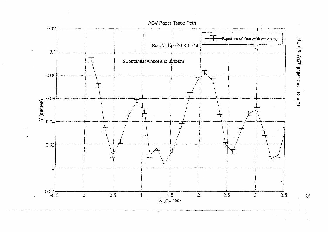
r;; ~ 10 E -
AGV Paper Trace Path 0.12~1 --------~------~--------~------~--------~------~------~------~
0.1
0.08
0.06
· · · · · , , Run#3, I 'I I Experimental data (with error b8<Sl
Kp=20 Kd=-118 1 . i • , I , • , •
•••• - ••••••• -. "' •• '- - ',C -- --. - """"" •••• ----r'" -----. --------....... r .... --...... -... _-. -.... ; .. -.-.. -- .. -" .... --. '--T' -.-.-.. _. -.... -.---. '-' r --. _. -.---.... -.. -------1-· -' -.-----.-... -.-... -
j Substanti~1 wheel slip eWident iii • • I ,. • t. , I I. , , tIt , I I , I I. ,
• t < • • t, , I ,. I
• t " ! ~ • -....... -~ ~"' .. ------.... . __ ......... -"' .. --._-_ ... - ... _----..... _-------- -- ------_ .... --- ............. -_ .. _ ........ -_ .... -------~.. ... ... ------- ....... ---"' ....... ----_ ..... -- ---~ .. ---- .. ------.---.......... -.. -~ -_ .. - .... ----_ .. • , • • I I ; t. I. · " .. ; •• I f · , . · . , . · . · , · , · , , , · , , . , , , , , , · , · . ,
~
>- 0.04
0.02
o ...L
-0.02'L-------~--------J-------~--------~--------~------~--------~------~ -0.5 0 0.5 1 1.5 2 2.5 3 3.5
X (metres)
~ ~.
P-oe I
>-~
't:l = 't:l ~ "'\I ..... "'\I = t')
$I>
~ = ~ t.I.)
-..J VI
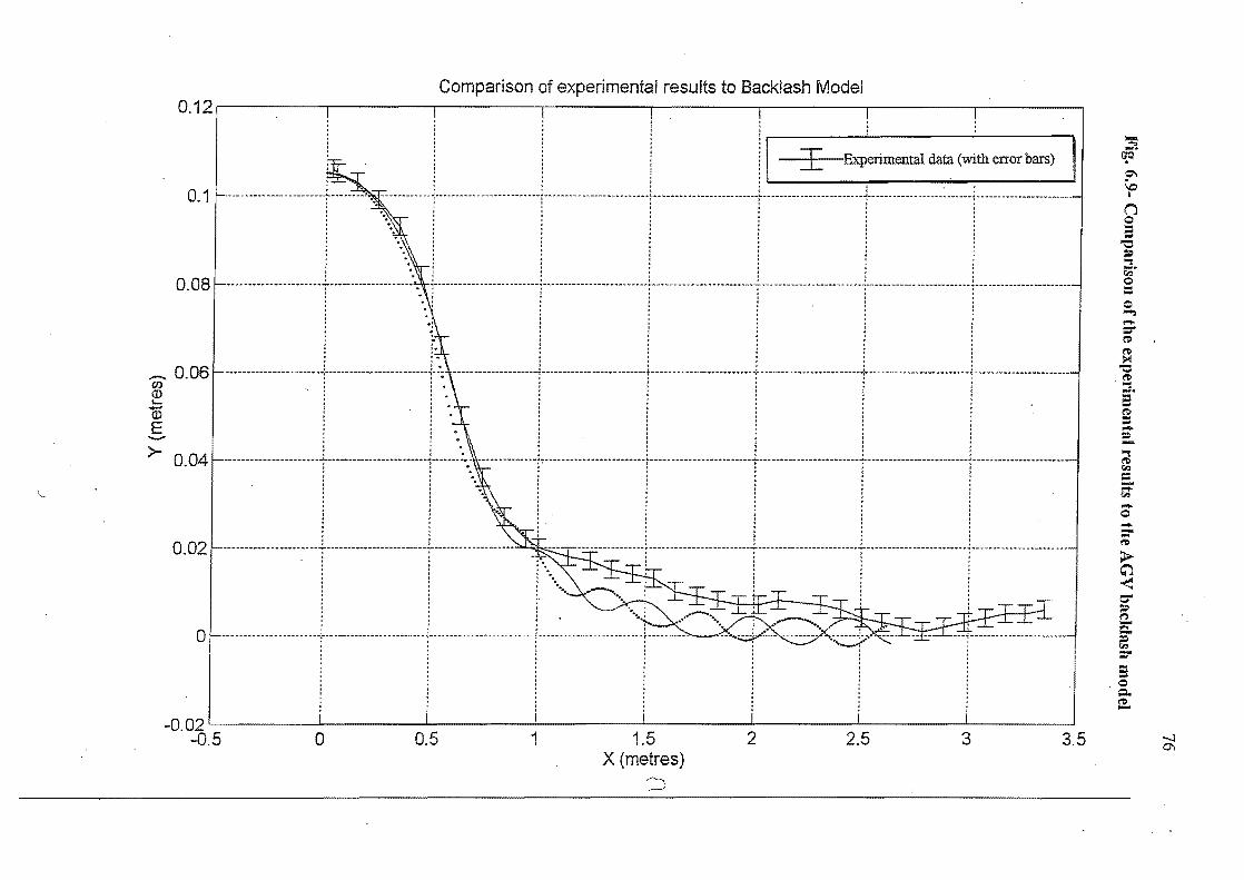
<D "0
o 2 ..c (/) ro
-0 ro CQ
.8 ~
::J (/)
~
.f!! c <D E
·c
<D a. ~ 4
-o C
o (/) ·c ro a. E
o () N
.... 0
Fig. 6.9-
Com
parison of the experim
ental results to the AG
V backlash m
odel
, , , , , , , , , 1 ,
76
·-1-~ ~ ---.. _--_ .... --~----r-------------.. ~ .. ,,-.. -r -"'--.... "., .... -----,.""''''1----.... -----.. --------~---" ,.~.-.......... -1"H'~" ... "
. """ ..... -1
I
I I
I f
I I
I I
• I
j I
I •
! !
! !
! I
I I
I I
I I
, I
t I
j ,
I I
I I
I t
I I
I t
I I
I ,
I I
j ,
I-,
I I
' I
, f
j
I ~
* I
I I
t j
I I
I I
I i
I I
I j
• I
I I
I I
I I
I j
t I
I I
I I
I I
• It,
i I
I I
I --4
------------............ ~ .. t---~------........ " ........ -~-................ -.... ,. ...... "'--1-" _'" ............ _______ ... " ~ .................. __ .. ~ t
I ,
I I
: :
I :
: I
t I
I I
• I
I I
I I
t I
• I
I I
I I
I I
• I
~ I
I I
I 1
I I
, ,
• I
! :
: !
!
1 !
! I
I I
t I
I I
.. ···············r···················r···· .. ···· .. ······-r··· .... ······· .. ···1'···················r·········· •
• •
f I
I •
• I
; I
I I
, ,
I I
t f
I I
I I
• •
I I
I t
I ,
• I
I •
I I
I I
I I
I I
I •
I I
• I
I
: !
: :
: :
t I
I I
I I
: :
: :
: j
I I
I I
, f
I ,
f I
I
~ .. ----.. --... ------",,~ .... -...... --........ _-_ .... ---f .... ,. "' ... ---_
¥., .... --~-~~~--
...... ~ .. -------
......... ,. ~-----~~-.-----...... ,. -
" ~ ........ ~
______ .... _
_ ""~~~~,, _ ~ '" _ .... ~ _
_ ~ .. _ .. _
_ _
" '"
' "
" .'
, .,'
':,
f i
1 i
! 1
t •
J ,
~ !
i ~
i :
I ,
I ,
I j
................. J .................... l ................... 1 ................... ), ................. ' .:: ............... !:,~ ...... _ .. _ .... '" _______ ~ ~
: ~
: ,
I l
, ,
I 'I
I t
j l
I •
t 1
t I
t j
t I
: :
: ~
I ,
• •
, I
• ;
I I I,
I I
, I
I
iii'
, .......... -... -.... -----_ .. ~-.. --_ ...... -. ----" -.. ~ .. -i ----..
_ ........ ! .. : ...... ~------.. -........ -_ .......... " ........ -...... ---........ " ...... _ ~_ ... _ .... _ .. ________ .. _ ~-f-.. __ ........ ___ .. __
M_
....
:,': :': . . .
i :
: i
: !
: :
! ~
; 1
I ~
i !
, ,
• I
i i
r f
i ;
! !
I ~
I I
I ,
_ .. -1----.. _--~
M
-.... -
'" "-'---t--...... -_ ........... ~'" .......... ;---.. -_ ..................... -.... 1 ...... ---_ .. ---.. -........ ,, __ t .. __ ..... _ .. _~ __ .. ___ .... _ .!_ • ___
M_
.... _
__
_ ..... _
._
Itt
I I
I I
• J
I I
• I
I I
• I
j
I I
; t
I I
: :
I :
: :
I I
I ;
f I
t •
I j
• •
I I
I I
I •
I 1
I I
f I
I •
I I
t I
I •
1 I
t I
I: I
I I
f I
i ~
1 i
i ~
I •
I I
I I
1 ~
~ i
i 1
.... ro
ill
""'" N
0
0 0
0 0
0 0
0 0
0 (S
9Jl9W) A
LO
N
LO
o o LO
NO
0
'
0 I
><
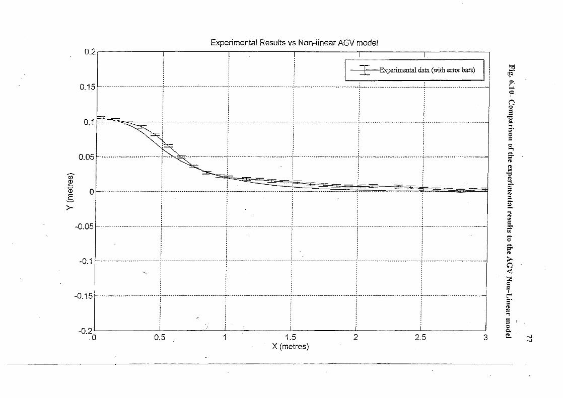
<"! 0
77
Fig. 6.10-
Com
par'ison of the experim
ental results to theAG
VN
oll-Lineal' m
odel
"......
j ~ It) ~ "-'
,
: i
, , ,
, ,
, ,
, , ,
, ,
, I
, ,
,
~ ~ .~ It)
~
, M
M~ M
_
k M
-
.... M
" "
'" .
. --~
.. -t ---.......... -.... ~"--"''' t -_ .. ,. .......... ----....
.. .. -_ .. ~------......... -i ...... -... _------""-... i,. .. ----............ -----1--~~ .... _ ............. .. :
: f
:::
: ::
l::
! ::
!::
! ::
:!:
j ~!
i!
1 It,
f I
,
i. i,!,
'"
I "
~ i
~ •
* I
I.
t
.: :
i ::!
l !!
1 i
l ~ .. ~---.... -~ ,,"'---.. '" --'O ~ .... "' .... ____________ ~ ........ __ ... ______
! ___ .............. __ ...... __ : __________ ........ _ .... : .. __ .. ,.. ..... ___ .. ____ .. _~ __ ~ .............. _ ...... .. I
, ,
I j
I I
I •
I I
, •
I
: :
t :
: :
: :
! :
i :
: :
~ !
! i
: !
! :
: I
! :
: :
I I
I I
I •
I I
I j
: :
: :
i, i,
!, :
: :
: •
I ,
I
, li !,
!, !
! i
i -------------l----
--1---------1---
--1____1_______ --I. --------___ J -------___ _
: :
: !
! 1
! i
1 1
,
!" [:
l: ~I'
i" ':
:,'
I I
f j
! !
i :
: !
: :
: :
: :
: :
: :
: !
, I
I j
, ,
': .. ' II:
I:: :
! :
:
! 1
i !
! :
: I
I I
• I
I I
, I
• •
: :
: :
: :
1 I
* I
( •
I I
.. -------.. --_ .. --:-_ .. ~ .. --" --.. ----... --~---.... ~ ........... ~ ~ ........ ~"" --.. ----~ ~ ~ ~ ..... i .. ~--~ .... ~ .. ~----...... t .... -----.......... ~--.... i _ .... ~-.... ~ _ .. ~,. ~ .. ~ -~ t ~ ~ .. _ .. -.. -,.,. ..... __
: :
: !
: :
: '
I 1
• I
I I
' Itt
, I
• '
I t
I I
I t
: :
: :
I :
:
: !
i :,1
1, !,
~, ,~
i 1
! I
I I
I
i j
! i
! !
i :
: :
i I
I I
I I
I •
I I
I
-----H_.i:: --------1:: .. -..... --_: ______ .......... 1 .. ______________ 1_ .. _______ ... _
. i ____ ._. _____ ... --J ____ . __ ... _ .. _. :
: :
: :
1 I
I i
I I
t I
I I
:: II
1 :
! :
: :
: :
: (
1
l::II. ! iii
l !
! i
! 1
I
i 1 ill
l()
'<""' LO
0
l()
T""
LO
T""
d 0
0 d
T""
d d
d I
d I
I
( S9
Jl9W
) A
LO
d
~o
d I
><
78
7. CONCLUSIONS
The objective of this thesis was to develop models of the AGV to exanune the
possibility of using the minimal AGV in situations where it has to travel in reverse.
This is analogous to the "Truck Backing" problem where the driver has to manoeuvre
a trailer into a space by reversing the truck. In the case of the minimal sensor AGV,
the lack of observable states would make the task more like backing a trailer with no
knowledge ofthe location of the trailer, only the position ofthe towbar.
The models presented in this thesis do not accurately' represent the AGV at the limits
of traction. However they do demonstrate a good correlation for low pelformance
AGVs in non-rigorous conditions, or well loaded AGVs on good traction sUlfaces.
In terms of the minimal sensor AGV s, the UOC AGV needs development of the
mechanical systems as much as the control systems. The reduction of bacldash in the
gear train would increase the performance envelope, as it would reduce the likelihood
of traction loss under heavy control effort. From the analysis of the simple linear
sensor case, the AGV is controllable in all states, but unknown in all but one, the guide
wire sensor location.
The number of additional sensors to add to. the AGV would be determined by the
pelformance requirements ofthe target AGV system:
(\) The addition of a guide wire second sensor pair at the back opposite the existing
pair would make the AGV bi-directiona~ and eliminate the reversing problem as it
could always be going forwards simply by using measurements from the 'leading'
pair of sensors.
• More adventurous application of the AGV requires greater investment in sensors.
To control the AGV near the limits of traction, it is necessary to include some
measure of the wheel speed at the very least. This would mean the addition of two
angular speed transducers on the DC motors or drive wheels. A simple solution
would be the addition of a 'chopper disc' to give some velocity feedback, as they
are fairly simple to interface with digital controllers. Alternatively, brushless DC
motors contain this information as part of the commutation command requirements.
79
<II Further, to completely control slip, it would be necessary to sense the relative
motion of the AGV with respect to the ground. This would be possible by using an
encoder on one of the castors, to indicate the actual speed of the AGV This
combined with wheel speed sensors would give a good indication of the state of the
AGV at all times, but would increase the cost of the unit markedly.
Two improvements to malee to the UOC Mle-II AGV would include the addition of
softer compound tyres for use on hard, painted surfaces, and the design of a gear train
with lower backlash. One possibility would be the design of a direct drive Brushless
DC motor for AGV and wheelchair applications. In terms of a minimal sensor AGV,
this would virtually eliminate the backlash effects but it would raise the complexity of
the control system significantly. This option is however under evaluation by wheel
chair manufacturers and will probably be available for future evaluation.
80
8. REFERENCES
[1] Steve Hampson, 1995, Non-linear predictive control of a hydraulic actuator, PhD
Thesis, University of Canterbwy, Christchurch, New Zealand
[2] David B Reister Francois G. Pin, 1994, Time optimal Trajectories for Mobile
Robots with Two Independently Driven Wheels, The International Journal of
Robotics Research, pp 38-53
[3] Nilanjan Sarkar, Xiaoping Yun, Vijay Kumar, 1994, Control of Mechanical
Systems with rolling Constraints: Application to dynamic Control of Mobile
Robots, The International Journal of Robotics Research, pp 55-69
[4] E. K. Boukas and J. P. Kenne, 1992, Autonomous Vehicle: A comparative Study
of Control Algorithms, European Joint Conference on Engineering Systems
Design and Analysis, pp 183-187
[5] A. Hamdy and E. Badreddin, 1992, Dynamic Modelling of a Wheeled Mobile
Robot For Identification, Navigation and Control, Robotics and Flexible
lvlanufacturing Systems
[6] W. Drodzd and H. B. Pacejka, 1991, Development and Validation of a Bond
Graph Handling Model of an Automobile. Journal of the Franklin Institute, Vol-
328 pp 941-957
[7] Z. Qu, D. M. Dawson, J. F Dorsey, 1994, A New class ofRoust Control Laws for
Tracking of Robots. The International Journal of Robotics Research, Vol 13 No
4 pp 355-363
[8] H. B. Pacejka, 1985, Modelling Complex Vehicle systems Using Bond Graphs.
The Journal of the Franklin Institute, Vol 319 No 1 pp 67-81
[9] Dean Karnopp, 1979, Bond Graphs in control: Physical State Variables and
Observers. The Journal of the Franklin Institute Vol 308, No 3 pp 219-234
[10]B. W. Johnson, J. H. Aylor, 1985, Dynamic Modelling of an Electric Wheelchair.
The IEEE Transactions on Industry Applications, Vol1A-21 pp 1284-1293
[11] Y. Y. Cha, D. G. Gweon, 1994, Real Time control using explicit dynamic
solutions of a two-motion-modes mobile robot. Proceedings of the institute of
lvfechanical Engineers, Vol 208 pp 157-167
[12]L. Borenstein, Y. Koren, 1987, Motion Control of a Mobile Robot Platform. The
Journal of Dynamic Systems, Measurement, and Control, Vol 1 09 pp 73-79
81
[13] Imai,K Fujiwara, Y. Kawashima, 1987, Advanced Automated Transport
System. Automated Vehicle Systems-International Trends in lvlamifacturing
Technology
[14]Kai Lui, F. L. Lewis, 1988, Control of a Mobile Robot with On-board
Manipulator. Robotics and Manufacturing - Recent Trends in Research and
Applications, ASME Press, Vol 4 pp 539-547
[15] Lennart Ljung, 1986-1991, Matlab System Identification Toolbox. The
Math Works Inc.
[16] Lennart Ljung, 1987, System Identification-Theory For the User. Prentice Hall
[17] Derek Ward, 1996, Design of a robotic finger, ME thesis, University of
Canterbu1)J, Christchurch, New Zealand.
[18]H. Overbye, 1989, Automated Guided Vehicle Mechanical Design. Bachelor of
Engineering Project Report #38
[19]R.J Kerr, 1989, Automated Guided Vehicle Electronic Hardware Design.
Bachelor of Engineering Project Report #22
[20]Julian SneIder, 1989, Automated Guided Vehicle System Software. Bachelor of
Engineering Project Report #46
[21]G.R. Dunlop and ID. Murphy, 1993, A universal pulse processing board for
instmmentation and machine controL Proc. NELCON'93, Auckland, Nell'
Zealand, Vol 1 pp171-178.
[22]A1an Blundell, 1982, Bond Graphs for Modelling Engineering Systems, Ellis
HOlwood
[23]The Math Works Inc, 1992, Simulink; Dynamic System Simulation Software -
Users Guide, The Math Works Inc.
[24 ]Phillips Semiconductors, 1994, 80c51 based 8-bit Microcontrollers, Phi /lips
Semiconductors.
[25]Intel Corporation, 1981, MCS-51 Family of Single Chip Microcomputers- Users
Manual, Intel Corporation.

APPENDIX A: AGV IVIICROCONTROLLER 'C' CODE
AGVAD.C
/* IMPLEMENTATION MODULE AGVADi Retrieves the values of the ADC from the Inputs in round robin
fashion and store the resultant values in the appropriate locations. It also enables the ADC to be used for other purposes by checking see if the AD conversion was initiated by these routines */
#include "AGVAD.H" #include <80c552.h>
/* VAR */ /* public vars */ unsigned char SensorValue[2]i
/* Functions */
void InitADC(void) {
} i
/* Clear the AD control register */ ADCON =OxOO,'
void GetSensorValues(void) {
) ;
InitADC()i
/* Set ADC to get Channel Sl */ ADCON = ChanSli
/* Start Conversion */ ADCON 1= OX08i
while (! (ADCON & OXl0))i /* Wait for an answer */
/* Store value in Sl*/ SensorValue[O] = ADCHi
/* Clear ADCI Flag */ ADCON "= OXl0i
/* Set ADC to get Channel S2 */ ADCON = ChanS2;
/* Start Conversion */ ADCON 1= OX08i while (! (ADCON & OXl0))i /* WAIT FOR ANSWER */
/* Store value in S2*/ SensorValue[l] = ADCHi
/* Clear ADCI Flag */ ADCON "= Oxl0;
/* END AGVAD.*/
AGVCONT.C
/* IMPLEMENTATION MODULE AGVCONTi */ /* This Module calculates the control signal to pass to AGVDrive
from the position of the AGV [module AGVPos] */ #include "AGVCONT.H"
82
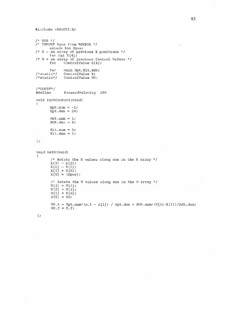
#include <80c552.h>
/* VAR */ /* IMPORT Xpos from AGVPOS */
extern int Xpos; /* X = an array of previous X positions */
far int X[4]; /* U = an array of previous Control Values */
far ControlValue U[4];
far /*static*/ /*static*/
Gain Kpt,Kit,Kdt; ControlValue Ri ControlValue UO;
/*CONST*/ #define ForwardVelocity 100
void Initcontrol(void) {
Kpt.num -1 ; Kpt.den 20;
Kdt.num 1; Kdt.den 8;
Kit.num 0; Kit.den 1;
} ;
void GetU(void) {
/* Rotate the X values along one in the X array */ X[3] X[2]; X[2] X[l]; X[l] X[O]; X [0] (Xpos) ;
/* Rotate the U values along one in theU array */ U[3] U[2]; U[2] U[l]; U[l] U[O] i U[O] UO;
83
UO.t UO.f
Kpt.num*(R.t - X[l]) / Kpt.den + Kdt.num*(X[O]-X[l])/Kdt.den; R.f;
} ;
AGVDRIVE.C
1* IMPLEMENTATION MODULE AGVDRIVE;*I #include "AGVDRIVE.H"
#include <80c552.h>
1* VAR *1 #define P~v.MForward P~l #define P~Turn P~O
bit DriveDisabled @ P4_BADDRi
/* CONST #define #define #define #define #define #define
*/ HalfDuty Oxff/2
ShortestPeriod OxOl LowP~O 20 HighP~O 236 LowP~l 20 HighP~l 236
void AllStop ()
) i
/* Set the Motors to stop *1
/* Set the P~ to half duty cycle *1 P~Forward HalfDutYi P~urn HalfDuty;
void InitDrive ()
) ;
/* Initialise the AGV Drive system, via the P~
/* Disable Drive */ DriveDisabled = TRUE; /* Set the P~ Period Prescaler*1 P~v.MP ShortestPeriod; 1* Set the P~ to half duty cycles *1 AllStop ();
void Drive (int Forward/int Turn) (
static far unsigned char ptO; static far unsigned char ptli
if (IDriveDisabled) {
/* Calculate the temporary P~ values ptO,l*/
and Port 4*1
/* It is inadvisable to perform calculations on the P~ Ports directly, as the DCMC will switch off power
84
to the motors if the P~ goes outside the recognised boundaries. Therefore it is necessary to use temporary
else {
J ;
variables */ ptO = (unsigned char) (Forward+ ptl = (unsigned char) (Turn - HalfDutY)i
/* Check the Ranges if (ptO > HighP~O) if (ptl > HighP~l) if (ptO < LowP~O) if (ptl < LowP~l)
of new P~ values */ ptO HighP~O i ptl HighP~l; ptO LowP~O;
ptl LowP~l;
/* Assign the Drive values to the P~ ports *1 P~Forward = ptO; P~Turn = ptl;
AllStop () ;
} ;
/* END AGVDRIVE.*/
AGVINT.C
/* IMPLEMENTATION MODULE AGVINT;*/ #include "AGVINT.H" #include <80c55Z.h> #include <intrpt.h>
/* ???FROM AGVDRIVE IMPORT DriveDisabled>????i */ extern bit DriveDisabledi
/* set the INTERRUPT VECTOR */
ROM_VECTOR(EXTIO,BumperInterrupt)i
/* function implementation */ void InitAGVInterrupts(void) ( /* Initialise AGV interrupts EXO */
EXO = TRUEi /* enable global interrupts */
EA = TRUEi } i
interrupt void BumperInterrupt(void) { /* Emergency stop routine - set PWM Channels to 50% and
- CLEAR Enable pin to DCMC */ PWMO = Oxff/Zi PWMl = Oxff/Z; DriveDisabled TRUEi EXO = FALSEi }
/* END AGVINT.*/
AGVLOOP.C
/* These functions use the Timed Control Loop using TimerZ*/ /* TZ is set as a FRC and an interrupt is generated off a
TZ compare. At each interrupt it is incremented by a value (ControlLoopPeriod) and re-loaded. */
/* NOTE: for this part of the program to operate properly, the vector for TZ's compare must be set to point to the stubControlLoop */
/* includes */ #include "agvloop.h" #include <80c55Z.h> #include <intrpt.h>
/* constants */ ROM VECTOR(CMPZINT,StubControlLoop)i /* set CMIZ to the control Loop */
/* variables */ unsigned char ControlLoopPeriod; void far (*ControlLoopFunc) (void)i
/* function prototypes */ void InitControlLoop(void)i void StartControlLoop(unsigned char,void far (*) (void))i void stopControlLoop(void) i interrupt void StubControlLoop(void)i
85
/* function implementation */
void InitControlLoop(void) /* Set up T2 and it's interrupt */ {
/* Set T2 as a Free Running Counter with a 16bit overflow period of around 500ms , fosc/12 + 1/2
TM2CON "" Ox04;
/* ensure that the interrupts are off */ ECM2 FALSE; CMI2 = FALSE; /* and that the flag is not set ... */
} ;
void StartControlLoop (unsigned char newcontrolLoopPeriod,
void far (*newControlLoopFunc) (void) ) /* Start T2's interrupt -
86
and load variable which will point to the Control Loop Itself*/
} ;
/** set up the Control Loop Variables */ ControlLoopPeriod newControlLoopPeriod; ControlLoopFunc = newControlLoopFunc;
/* Set up the compare registers */ CML2 OxFFi CMH2 TMH2 + ControlLoopPeriod;
/* enable compare interrupt */ ECM2 TRUE;
/* start timer */ TM2CON I OxOl;
/* enable interrupts */ ei () ;
void StopControlLoop(void) /* Stop T2's {
} ;
/* disable compare interrupt */ ECM2 FALSE; /* turn off timer */ TM2CON &= OxFCi /* clear flag */ CMI2 FALSEi
interrupt void StubControlLoop(void) (
*/
/* clear the T2 compare and add the period
} ;
to the compare register*/ CMI2 = FALSE; CMH2 += ControlLoopPeriod;
/* call the control Loop Function */ (ControlLoopFunc) ()l
AGVPOS.C
/* VI.4 VI.3 converted from MODULA2 to C */ /* Calculates the position of the AGV's Sensor from the sensor inputs
incident at the AD channel */
#include "AGVPOS.H" #include <BOc552.H> #include <stdlib.h>
1* ???FROM AGVAD IMPORT SensorValue; ???*I extern unsigned char SensorValue[2];
1* defines *1 #define S SensorValue #define Slmax BO #define SensorMinimum 4
1* public vars *1 int Xpos; bit LostWire; bit signX;
I*private vars *1 unsigned char gS; 1* Greater Sensor value *1 unsigned char lSi 1* Lesser Sensor Value *1
1* TYPE */ typedef unsigned char LUColumn [21];
1* CONST *1 I I LUColunm LuX= {0,6,13,19,25,32,3B,45,51,5B,64,70,
77,B3,90,96,102,109,115,121,127); II II II II II II II
LUColunm LuS2= {BO,121,151,lB6,214,237,240,226,210,164, 132,109,B5,67,51,41,32,25,19,14,10};
LUColumn LuS1= {BO,70,55,40,30,21,14,11, 7,5,3,2,1,1,1,0,0,0,0,0,0);
1* function implementation *1
void GetXpos(void) { I*VAR* I I I char i;
II COlnmented out all the 'lookup table' stuff, II let's have a go a simple proportional control II Using the sensor level differential ...
II
gS max(S[O], S[l]); lS min(S[O], S[l]);
1* Decide if the wire has been Lost *1 if ((gS < SensorMinimum) && (lS < SensorMinimum)) {
else {
) ;
LostWire = TRUE;
LostWire FALSE;
1* Deduce the sign of X *1 if (S[O] < S[l]) {
else {
) ;
signX = TRUE;
signX FALSE;
II 1* Decide which variable, lS or gS, will II be used on the lookup table *1
87
II if (gS < Slmax) II {
II for(i = 0; i <= 20 ; i++) II {
II if (LuS2[i] > gS) II {
II Xpos = LuX[i]; II ) ; II ) ; II II else II {
II for (i = 0; i <= 20; i++) II {
II if (LuS1[i] > lS) II {
II Xpos = LuX[i]; II ) ; II ) ; II ) ; II II if (signX == TRUE) II {
II Xpos = -Xpos; II
Xpos = S [O]-S [1] ; )
#undef S 1* END AGVpos.*1
AGVSER.C
1* IMPLEMENTATION MODULE AGVSER; *1 1* simple module that reads 8 bits AID on the 80C552
and dumps out serial port *1
#include "AGVSER.H" #include <80c552.h>
1* CONST *1 char HexTbl[] = {"0123456789ABCDEF");
void SendP(register char Ch) { 1* wait until the Serial transmit buffer is empty*1 while (! (TI)); 1* Stop bit transmitted??*1 TI = FALSE; SBUF = Chi
) ;
void SendHexH(register unsigned char HexB ) {
SendP(HexTbl[HexB % 16]); 1* Send hH Nibble *1 ) ;
void SendHexHH(register unsigned char HexB ) { . SendP (HexTbl [HexB I 16]); 1* Send Hh Nibble *1
SendP(HexTbl[HexB % 16]); 1* Send hH Nibble *1 ) ;
void SendOxDDD(char num) 1* Send a byte to the serial port in signed Decimal Form *1 {
if ( num < 0) {
S endP ( I - I ) ;
num = -num;
88
else SendP('+');
SendHexH(num /100); num = num % 100; SendHexH(num /10); num = num % 10; SendHexH (num) ;
void SendINT(int i) {
} ;
if (i < 0) {
SendP ( , - , ) ; i = - i;
else SendP ('+'); SendHexH((unsigned char) (i / 10000)); i = i % 10000; SendHexH((unsigned char) (i / 1000)); i = i % 1000; SendHexH((unsigned char) (i / 100)); i = i % 100; sendHexH((unsigned char) (i / 10)); i = i % 10; SendHexH((unsigned char) (i));
void InitSerial(void) {
TMOD = Ox21; /* TIMER 1 8 bit Autoreload Timer 0 16 bit */
TH1 = OxOFD; /* for 9600 baud 11Mhz */
*/ /* SOCON = 50H; /* 8 bit UART, SCON = Ox50; TR1 TRUE;
No Parity Timer1 baud control, Rx ON*/
/* start Tl */ TI = TRUE; /* SET TI-transmit interrupt flag, fool SendP */
} ;
void Wait10mS(void) { register int DP = 1024;
while (DP) DP--; } ;
void BOL ()
} ;
/* Send Carriage return */
SendP (OxOD); Wai t10mS () ;
void NEWLINE ()
} ;
/* Send Carriage Return - Line Feed */
BOL () ; SendP (OxAO); Wai t10mS () ;
/* END AGVSER.*/
89
PLAYTIME.C
/* playtime.c */
1* small program for the AGV to run on the OPEN day *1
1* The AGV will exhibit a simple behaviour, travelling to the end of the guide wire and spinning around until it re-discovers the wire and continues off along the wire *1
#include "AGVDRIVE.h" #include "AGVCONT.h" #include "AGVPOS.h" #include "AGVAD.h" #include "AGVINT.H" #include "AGVLOOP.H" #include "AGWARS.H"
#include " .. \lcd\LCD.h" #include " .. \lcd\events.h"
#include <stdio.h> #include <80c552.h> #include <intrpt.h>
1* defines *1 #define JIFFYTlME 3000 #define COOEE Ox60 #define CNTRLPERIOD OxlO #define TURNS PEED Ox20 #define CRAWLS PEED Ox20 #define WALKS PEED Ox40 #define RUNSPEED Ox65 #define CLOSETOHOME Ox30
1* variables *1 varT varKdt num varT varKdt-den int turn;
{ "Kdt. num" , &Kdt. num, INT I; {"Kdt.den", &Kdt.den, INT};
/* function prototypes *1 void InitEveryThing(void); void ControlClosedLoop(void); void (void); void (void); void (unsigned char);
1* function implementation *1
void main (void) {
InitEveryThing();
1* Wait for the button press to start *1 LcdPrintAt(1,5,"-=<AGV MK2>=-")i
LcdPrintAt (2, 2;" [ANY KEY TO BEGIN] ") i while (!IsEvent())i LcdCls();
AGVChangeVar(&varKdt num); AGVChangeVar (&varKdt::::den) i
DriveDisabled= FALSE; Delay(60)i StartControlLoop(CNTRLPERIOD,ControlclosedLoop);
while (TRUE) {
/*-- Go to the end of the guide wire -- *1
90
/* Ahead slow, the AGV over the center of the wire */ R.f CRAWLSPEED; R.t = 0;
while (!LostWire) (
} i
UpdateScreen () ; LcdPrintAt(l,l,"FORWARD ff
);
/* stop 'cos we've lost the wire */ R.f = 0;
/*-- Spin around 'till the wire is found again --*/ /* suspend the */ startControlLoop(CNTRLPERIOD,UpdateInputs);
if (signX = FALSE) {
else {
} ;
turn -TURNSPEEDi
turn TURNSPEED;
/* set turbines to speed and SPIN, no forward /* spin until it detects the wire */ do (
LcdPrintAt(l,8,"SPINNING") ; ();
Drive(O,turn)i while ((COOEE > SensorValue[O)) && (SensorValue[l) <
COOEE) ) ;
} ; } ;
/* and center on the wire */ R.t 0; R.f 0;
Kpt.num = -Ii Kpt.den = 4;
StartControlLoop(CNTRLPERIOD,ControlClosedLoop);
/* until we're within COOEE */ while ((CLOSETOHOME < Xpos) && (Xpos > -CLOSETOHOME)) (
} i
LcdPrintAt(1,2,"CENTERING"); UpdateScreen () ;
Kpt.den = 10;
void {
(void)
} ;
/* Initialise the various systems */ Lcdlnit()i InitDrive(); InitControl(); InitADC(); InitAGVInterrupts(); InitControlLoop()i Ini tEvents () ;
void ControlClosedLoop(void) {
GetSensorValues(); Getxpos (); Getu () ;
91
*/
Drive(UO.f,UO.t); } ;
void Updatelnputs(void) (
} ;
GetSensorValues(); Getxpos();
void Delay(unsigned char /* Delay a number of {
} ;
register unsigned int j;
while (jiffs--) {
) i
j = JIFFYTIME; ':,hile (j ) {;} ;
void UpdateScreen(void) {
LcdGoto(l,2);
Jiffy
LcdPrintlnt ((void -k) (&Xpos) ) i LcdGoto(6,2)i LcdPrintByte(&SensorValue[O] ); LcdGoto (11,2) ; LcdPrintByte(&SensorValue[lJ)i
} ;
1/60 sec */
AGWARS.C
/* AGWARS.C */
/* This module implements the variable adjustment program via the keyboard and LCD screen on the AGV */
/* It enables the user to change variables within the program provided they are listed in the program at compile time */
/* includes */ #include <80c552.h> #include <stdio.h>
#include nagvvars.hn #include n .. \lcd\lcd.h" #include " .. \lcd\events.hn
/* defines */
/* variables */ char varstr[6];
/* function prototypes */
void AGVChangeVar(varT *);
/* function code */
void AGVChangeVar(varT *var) (
register char bytel,byte2; char DONE = FALSE; register void far *baddr;
InitEvents();
while (!DONE) (
baddr = var->addr;
LcdPrintAt (1, l,var->name) ; LcdPrintAt(l,14,nOx ") ; LcdPrintAt(2,l,"Oxl00[-] [+]Oxl[-] [+]"); LcdGoto(16,l);
switch (var->type) (
} ;
case INT:
} ;
LcdPrintInt((int *) (baddr)); break;
case BYTE: {
} ;
LcdPrintByte((char *)baddr); break;
switch (IsEvent()) {
case Ml: {
* (char *)baddr 1; break;
) ; case M2:
93
*(char *)baddr +~l; break;
} ; case M3: {
} ;
if (var->type break;
case M4: {
INT) * (int *)baddr OxOOl;
if (var->type break;
INT) * (int *)baddr += OxOOl;
} ;
) ; case OK:
DONE = TRUE; case CANCEL:
DONE = TRUE;
}; 1* end while !done *1 LcdCls () ;
}; 1* end AGVChangeVar *1
94
APPENDIX UPPORT PC 'C' CODE
IDSYS.C DATA LOGGING UTILITY
II Here's a program to log the time history of the velocity of II tWQ channels of the AGV conmtrol system.
II IDSYS.C, logs data from the UPP counters and AD channels and II stores it to a file for processing in MATLAB.
1* The user will nominate a logging period and frequency. The program will warn if theses are not feasible values. The program will present a summary of the logging data and
prompt the user to begin input.
The User will operate the joystick control in a p-random fashion The Program will periodically determine the state of the system,
recording the DCMC input and the motor speeds *1
95
1* LOGLEG.C Log data points from the UPP into the PC memory for download*1
#ifndef #error #endif
large memory model to link with the PWML.lib library
#include <stdio.h> #include <alloc.h> 1/include <stdlib.h> #include "pwm.h" #include n\upp\upp.h" #include <conio.h> #include <dos.h> 1* for () *1
1* program defines and constants *1
j~define UPPADDR Ox0232
1* global variables *1 int *PWMdataOi int *ADdataOi int *PWMdatali int *ADdata1;
int datareadyflagi unsigned long int numsamples; unsigned long int sample;
char DATAFORMAT[]={"%9.5f\t%8i\t%8i\t%8u\t%8u\n"}; char TOBEGIN [] = ( "BEGIN" } i char TOEXIT []={"EXIT"}; char TOCONTINUE [] = {"CONTINUE"} ; 1* read the counter and stuff the value into a variable *1 void Timerlnterrupt(void) {
file
if (sample < numsamples) {
II Set the ADO scans going (hopefully) UPPStartAD(UPPADDR,ADO\STARTAD); delay (1) i I I delay 1 millisecond something to do 'ltd th the . c
Ilget Encoder positions PWMdataO [sample]=ReadSingleEncoder(O);
96
file
else {
Ilget AD \\fhile (UPPIntStatAD (UPPADDR) ) ; /* AAAAAAAAAAAAAAAAAAAAA */ 1* this is broken I!! doesn't return anything meaningful*1 delay(1) ; ADdataO [sample]~UPPReadAD(UPPADDR,ADO);
UPPStartAD(UPPADDR,AD1I STARTAD) I delay(1); II delay 1 millisecond something to do with the
PWMdata1 [sample]=ReadSingleEncoder(l);
while(UPPIntStatAD(UPPADDR)) ;
(1) ; [sample]~UPPReadAD(UPPADDR,AD1)1
return;
1; return;
1* Detect the existance of the UPP and the version number of the software *1 void DetectUPP(void) {
BOARD card; int chips found;
chipsfound=UPPFindBoard(&card);
("UPP chips found: %i \n", chipsfound); printf("UPP software version V%i",UPPVersion());
("\n[ANY KEY TO CONTINUE]"); ( ! kbhi t () ) ;
void PressAnyKey( char *msg) {
if (kbhit()) getch(); II clear the buffer of a characher ... ("\n[PRESS ANY KEY TO %13) ",msg) ;
();
1* begin the main section *1 void main() {
int i; unsigned int interruptsteps; float numseconds, FILE *outputfile; char outputfilename[100)i char comment[163]i struct date d; struct time t; unsigned long int tSI
.c
\n");
datareadyflag 0; PWMdataO=NULL; ADdataO =NULL; PWMdata1=NULL; ADdata1 =NULL;
clrscr(); DetectUPP();
1* get the approximate timestep from the user *1 do (
clrscr () ; (" -=«Encoder and Control Signal Data
(" Enter Timestep{ms): "); } while (! {scanf ("%f", ×tep) ) ) ;
V1.0»=-
II of limited resolution due to delay{)s in the interrupt routine
if (timestep < 5) { printf ("\nTimestep Limited to 5ms, due to Interrupt
resolutionH); timestep = 5; PressAnyKey(TOCONTINUE); }
interruptsteps = (unsigned int) (timestep/3. 25*1000) i
1* get the sample time from the user *1 do {
clrscr () i printf{" Enter Sample period(s): ");
while (! (scanf (H'bf" , &numseconds) ) ) i
1* calculate the number of samples *1 numsamples = (long unsigned int)lOOO*{numseconds I timestep); if (numsamples <~ 0) (
printf(Hlnvalid negative numsamples")i return;
PWMdataO ADdataO PWMdatal ADdata1
(int*) malloc(sizeof{int)*numsamples); (int*) malloc(sizeof(int)*numsamples); (int*) malloc(sizeof(int)*numsamples); (int*) malloc(sizeof(int)*numsamples);
1* bug out if it's a bad pointer allocating memory*1 if «PWMdataO == NULL) I I (ADdataO==NULL)
97
I I (PWMdatal NULL) II (ADdata1==NULL) )
(
) ;
printf{"error malloc'ing the data exit{l);
1* things start getting a bit hairy here .. . *1 1* install the encoder *1 InstallEncoder(2); SetEncoder(O,O); SetEncoder(l,O) ; 1* install the timed interrupt vector *1 InstallTimerlnt(TimerInterrupt);
) ;
/* purtyfy the screen */ clrscr () ; printf (" SUMMARY: \n") ; printf("Desired Timestep(ms) :%f\n",timestep); printf("Actual Timestep(ms) :%f\n",interruptsteps*3.25/1000); printf ("NumSamples: %u\n", numsamples) ; printf ("NumSeconds: %f\n" ,numseconds) ;
PressAnyKey(TOBEGIN) ;
sample =0; datareadyflag = 0;
StartTimerlnt(interruptsteps);
while(!datareadyflag) (
} ;
gotoxy(1,8); printf("SAMPLE: \t%u",sample); printf("/\t%u\t",numsamples);
UPPStopAD(UPPADDR) ;
StopTimerlnt();
RemoveTimerlnt();
/* OK so we got the data, now to put it somewhere .. */ do (
there is */
/* get a filename */ clrscr () ; printf("Output file name please:"); scanf("%s",outputfilename); /* check to see if there is a file of that name ... go back if
}while ((NULL != fopen(outputfilename, "rt")));
outputfile = fopen(outputfilename,"wt");
printf("Comment:"); comment[Oj=160; /* set the maximum string length */ cgets(comment); printf("\n") ;
getdate (&d) ; gettime(&t) ;
fprintf(outputfile, "DATE:%d/%d/%i",d.da day,d.da mon,d.da year); fprintf (outputfile," @%d:%d\n",t.ti_hour,t. ti_min) ; -
fprintf(outputfile,"COMMENT: %s \n",&comment[2j);
for (i = 0; i < numsamples; i++) (
char WannaSee = 1;
float time;
if (kbhit()) WannaSee = 0;
time = (float)i * (float)interruptsteps * 3.25e-6;
98
if (EOF == fprintf(outputfile,DATAFORMAT, time,PWMdataO[ij,PWMdatal[ij,ADdataO[ij,ADdatal[ij))
} ;
}
(n/nError writing data to:%s",outputfilename); exit(l);
99
if (WannaSee) printf(DATAFORMAT, time,PWMdataO[il,PWMdatal[iJ,ADdataO[iJ,ADdatal[i]) ;
else (
} ;
} ;
gotoxy(l,l); printf("-=wRiTiNg to fI1E=-"); gotoxy(l,l); printf ("=-WrltlnG To FiLe-=");
printf ("\nData vlritten to: %s", outputfilename) i
PressAnyKey(TOEXIT);
/* all done - tidy up*/ clrscr()i
/*close the file*/ fclose(outputfile);
/*free the malloc'd memory*/ free(PWMdataO); free(ADdataO); free(PWMdatal); free(ADdatal)i
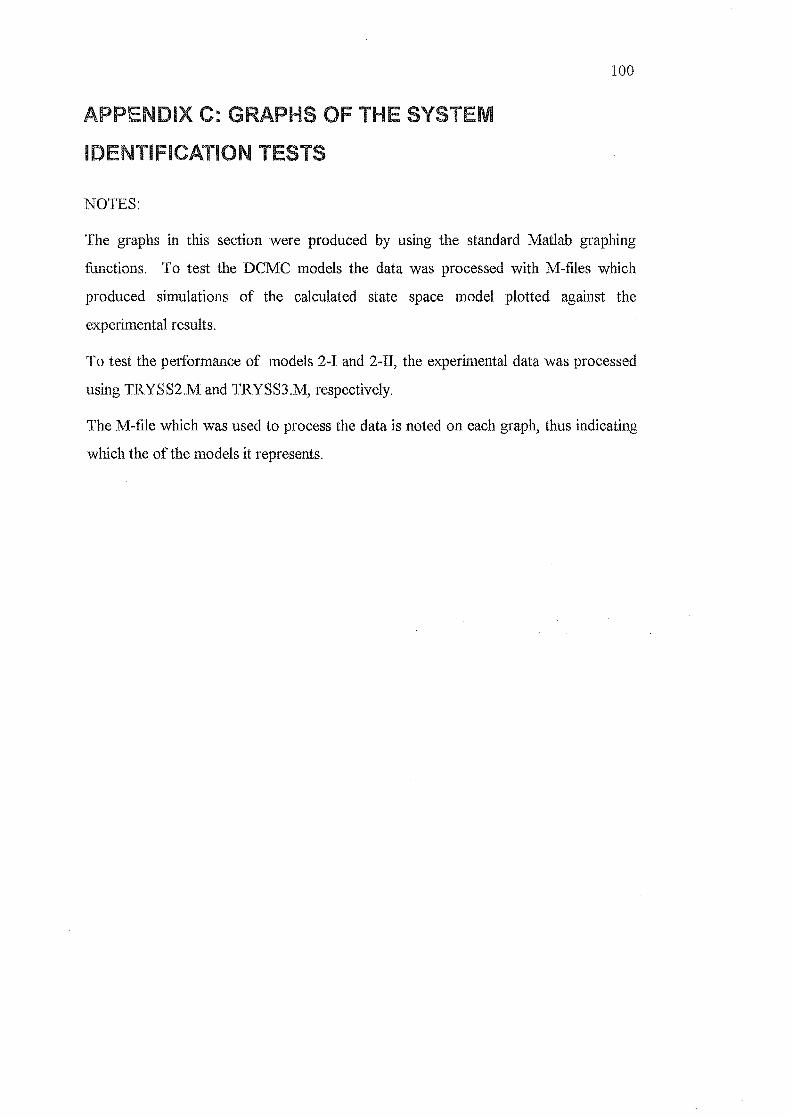
PEN IX C: GRAPHS OF THE SYSTEM
IDENTI ICATION TESTS
NOTES:
100
The graphs in this section were produced by using the standard Matlab graphing
functions. To test the DCMC models the data was processed with M-files which
produced simulations of the calculated state space model plotted against the
experimental results.
To test the performance of models 2-I and 2-II, the experimental data was processed
using TRYSS2.M and TRYSS3.M, respectively.
The M-file which was used to process the data is noted on each graph, thus indicating
which the of the models it represents.
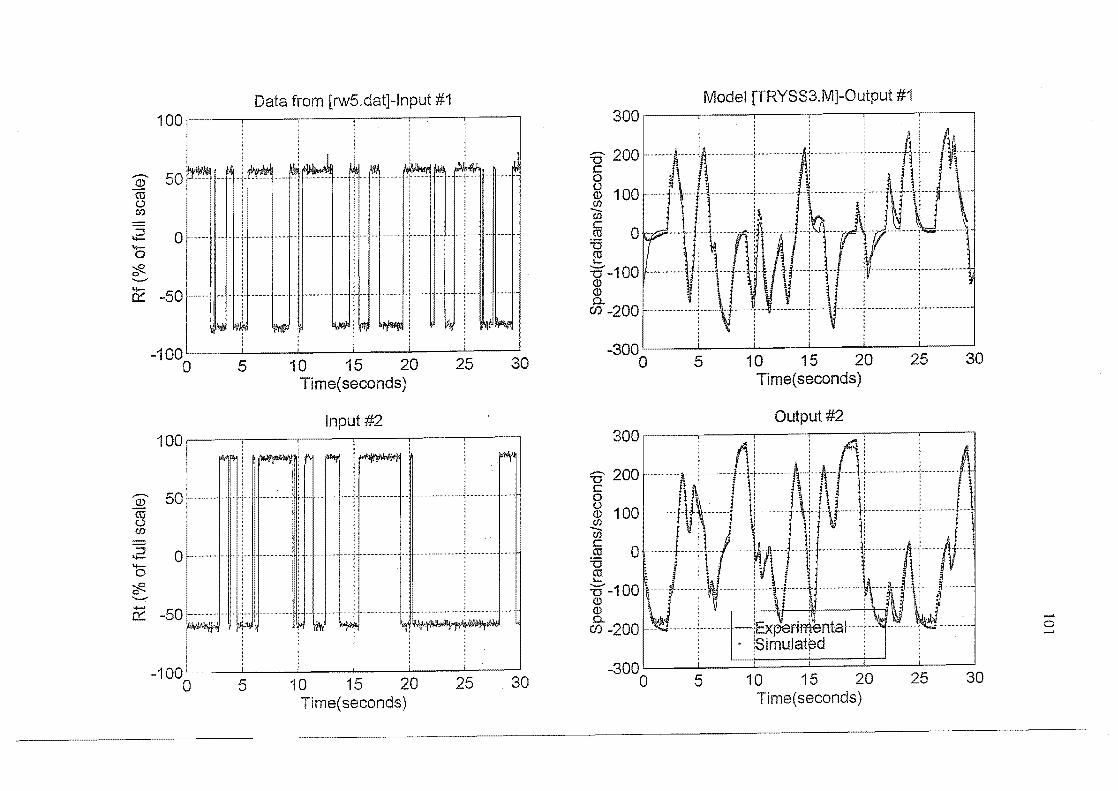
Data from [rw5.dat]-lnput #1 100" ----r---~----.---~----~--~
ill 50~----ro () 00
.2 0,",--4-o
:::R o .........,
n:: -50
-1DOLI ____ ~ ____ L-__ ~ ____ ~ ____ ~--~
D 5 10 15 20 25 30 Time( seconds)
Input #2 100.---~-~--~-~-~-~
ill 50 ro () w
o
-50
-100 o
j'\" .r¥
'1-
+ --~+---------~, -}~ ----- -" --_. -; -""-. ---< ----
~\f---- ---IIQ--W---~ 1;'-'-1' rP-: .... 17'
5 10 15 20 30 Time(seconds)
------,.
Model [TRYSS3.M]-Output 300~1 --~----~--~----~--~--~
13' 200 c o hl 100 C/)
in c .~ 0 1:1 ~ :0-100 (I) (I) 0..
CI) -200
~---~- ~--~ ~~ -{A ------ --- --- ~ ~ ~ -------
-------~-- -,- -i --- ----" -' f -- --,--
-300IL----~--~----~----~--~--~ 10 15 20 30 o 5
Time( seconds)
Output #2 300,-----.-----,------,---,-----,-----,
13' 200 c o as 100 C/)
in c .~ 0 1:1 ~.
:0-100 (I) (I) 0..
if.) -200
-300 ~_...L.--==t::===t:===±=__~ __ 10 15 20 25 30 o 5
Time( seconds)
>-' o >-'
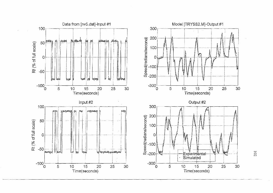
ID ~ en
....... a 'if!.
1
...... 0::: -50
-100 o
Data from [rvv5.dat]-lnput #1
5 10 15 20 25 30 Time( seconds)
Input #2 100" --~----~--~----~--~--~
ID 50 ro o UJ
.2 0 '0 :::R o
C2 -50 I------+-H~--H+----
-100~t ----~--~----~----~----~--~ o 5 10 15 20 25 .30
Time(seconds)
Model [TRYSS2. M]-Output #1 300" ----~--~--~----~--~--~
S 200 c o ~ 100 U) -U) c .~ 0 "0 ro s....
:0 -100 ill (I) CL en -200
-300 o 5 10 15 20 25 Time( seconds)
Output 300,- - ,
S 2001---------.--+--C o ~ 100 ~ c .~ 0 "0 ro s...
:0-100 ill ill CL
en -200
-300 o 5
: '« :\1 -fExperirnlEmta~--- ... ,,---.----
iSimulat~d
10 15 20 25 Time( seconds)
-,\---
30
30
....... o N
100
...-... 50 (l)
co 0 en
4-0
:::R 0
~
(i) co o en
.2 4-o
:::R o
C2
0
-50
1
00 o
-100 o
Data from [rw22.dat]-lnput #1
-~ - --- -- -~- - - ~ ~ ---- w~ _____
- ---- --- -I'"~----
, ,
, , ,
i 5 10 Time( seconds)
#2
5 10 Time( seconds)
---~- -- -
15
.15
300
'5' 200 c o <.) (])
~ 100 (/) c ro :0 ~ 0 ........ 'U (]) (])
g.-100
-200 o
3001-
Model [TRYSS3.M]-Output #1
5 10 Time( seconds)
Output #2
_ - Experimental I A -g 200 H--·----S~mu~ated--hr----t---fl-\--------J\-c-------o <.) (])
~ 100 (/) c ro :0 ~ ........-'U (]) (])
g.-100
15
-200~1 ----~--~--------~----~~ o 5 10 15
Time( seconds)
>-" o w
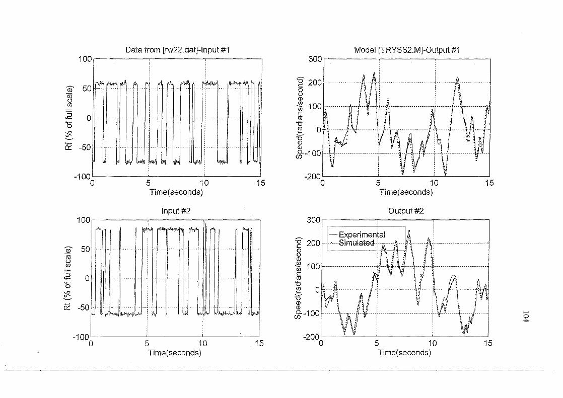
100
.-- 50 (j)
ro 0 en
:::'l 4--0
~ 0
4-
0:::
.......... (!)
ro 0 CI)
::J 4-4-0 ~ 0
...... 0:::
0
-50
-100 o
100
50
0
-50
-100 o
Data from [rw22.dat]-lnput #1
._- f w~~ __ -~ ~ ~ ---" ~- -- -- ---- . --- -~-- -- -~- -- ~-
--- ---- -- --- - -- -----, I ... ..... .. u ... .... ...... .. . -
i
5 10 15 Time( seconds)
Input #2
J if .. " C ~ , ~ -- ---- r-"--- -f- --- .. --- ---- - ---------- -
I J - --- .. - -- --- 1----- -1-- ---- - - --- ------- - ---
i I I l ,IU~ ~U --
5 10 _ 15 Time(seconds)
Model [TRYSS2.M]-Output #1 300,~--------~--------~--------~
B 200 c o (J (J)
~ (J)
c co =u ~ 0 .......-
"'0 (l) (l)
g.-i00
-200~' --------~----~----~~----~ o 5 10
Time( seconds)
Output 300 r---
,,---------+
..- - Experimental • -g 200 H--· .. --S~rnlflated+1\---"f:r---~-t-------H+-----o ' (J (l)
~ 100 f--_ ............ .. (J) c co =u ~ --"'0 (l) (J)
g.-100
-200 o 5 10 Time(seconds)
15
15

..-... (])
tIJ 0 en
::::R Q "'-"
C2
100 ,
50
0
-50
i"
-100 o
Data from [rw21.dat]-lnput #1
rI /11 ~ ,"'II' ~ .; -~ fiJ.1~ Iw.+ 1\\I>\1IJ , ~~ --r-- -- --- I-- -- - - ~ -- *~ ~-- -
1/ !
- 1-- -- --~ - - --._-- ------~ - -- -+> ----- . ~- ~ - ~- -
I. --t-- -- ----- - ------1--- -
~ ~Jl' ~ \;IJ"I hI l'IIII I\'
5 10 Time(seconds)
15
Model [TRYSS3.M]-Output #1 300f----------~----------~---------.
::0 200 1-------------------C o o (!) U)
en c .~ 0 v ~ :0 -100 (!) (!) Q.. (f) -200
-300~' --------~----------~--------~ o 5 10 15 Time(seconds)
Input #2 Output #2 100 I 200 r-, -------,------,-------,
..-... (])
co 0 en
4-0
"#-"'-" +-'
0:::
50
0
-50
-100 o
.~
5 10 15 Time(seconds)
::0 c o o (!)
~ ffi 0 :0
Time( seconds)
I-'
o VI
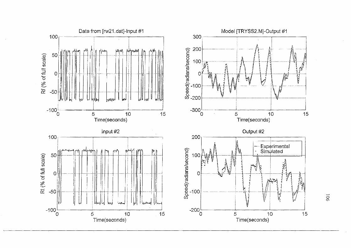
...-... (l)
co u (J)
::J ....... ....... 0 ~ 0 ..........
~
100
50
0
-50
00 o
Data from [rw21. dat]-Input #1
~-~I--~ ~.! tJo , I
----- 1--· - -
Jl. I ~ .---- -~- --- -+ . ----- ~
--r--
It'" ~ II> ~
5 10 15 Time(seconds)
Input #2 100
1 i : l~ : ~
(j) 50 co u (/)
..2 0 '0 ~ o '-"
~ -50
~n--rl--~-~l~---~--(1---n-----rr m-- Y*
---j,--+ + -. -J-- --~+! --+~ ++--+ ---1--- --I-~-· I------+HI·-
f ----- ----H --++---j ----;-~" - - -,-> ->--~- -->-- -.. ---- /-----+Ht----
l-wJl..j~ ~ \,<I ~\!~
-100~--------~--------~------~ a 5 10 . 15
Time( seconds)
Model [TRYSS2.M]-Output #1 300,1 --------~--------~--------~
U 200 c o ~ 100 ((J
(f.i c .~ a -0 co '-
::0--100 (l) (l) a...
(f) -200
-300'o 5 10 15 Time( seconds)
Output #2 200 1, --------:-------~--------~
...-... -0
§ 100 u (J) ((J
(f.i
§ a TI co ''-' -0 (J)
(J) -100 a... (f)
~OO'~--------~--------~--------~ a 5 10 15
Time( seconds)
....... o 0\
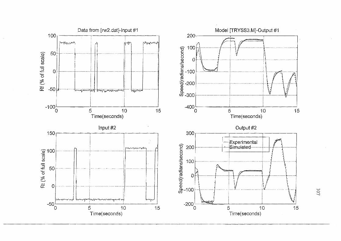
Data from [rw2.dat]-lnput #1 1
....-... ID (lJ (.) W
::::i 0 "'-
'0 ~ 0 --(2 -50
-100~1 --------~----------~--------~ o 5 10 15 Time( seconds)
Input #2 150~j --------~----------~---------.
ill 1 00 1---------------1 ro (.) U,)
..2 50 b :.:R o --~ 01--------------1
-50~1 --------~----------~--------~ o 5 10 15 Time( seconds)
Model [TRYSS3.M]-Output #1 200~j --------~--------~------~
B 100 c o ai 0 ~ ffJ C .~ -100 "0 ~ u-200 (]) (]) a.. en -300
400~j --------~--------~------~ o 5 10 15
Time( seconds)
Output #2 300~--------~--------~--------~
B 200 c o () (])
~ 100 ffJ C ro
~ 0" ......... "0 (I) (I)
c% -100 I--+-----------r
-2001.- =-o 5 10 15
Time( seconds)
........ o -.J
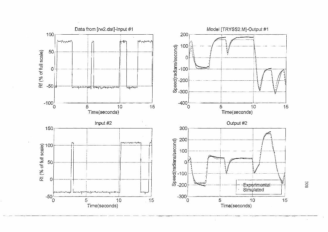
..-... cD co 0 U)
::J "<-"<-0
::R e ..........
~
1
-50
-100 o
Data from [rw2.dat]-lnput #1
5 10 15 Time( seconds)
Input #2 150 r·------,.-----,-------,
0)100 ro 0 U)
50 ...... 0
::R e .......... -+-'
0 IX ~ ,-- .------~--- .
-50 1
0 5 10 15 Time( seconds)
2001
..-... 10011: -0 u;. C o o (l)
~ c co -100 '5 co I-
::0-200 (l) (l) Q.. (j) -300 1----------.. -
Model [TRYSS2.M]-Output #1
~OO~I --------~--------~--------~ o 5 10 15 Time( seconds)
Output #2 300,~--------~----------~--------~
'5' 200 c 0
~ 100 U) -U)
c 0 co
'5 co l-
::0-100 (l) (l) Q..
Cf) -200
-300 0 5 10 15
Time( seconds)
-' o 00
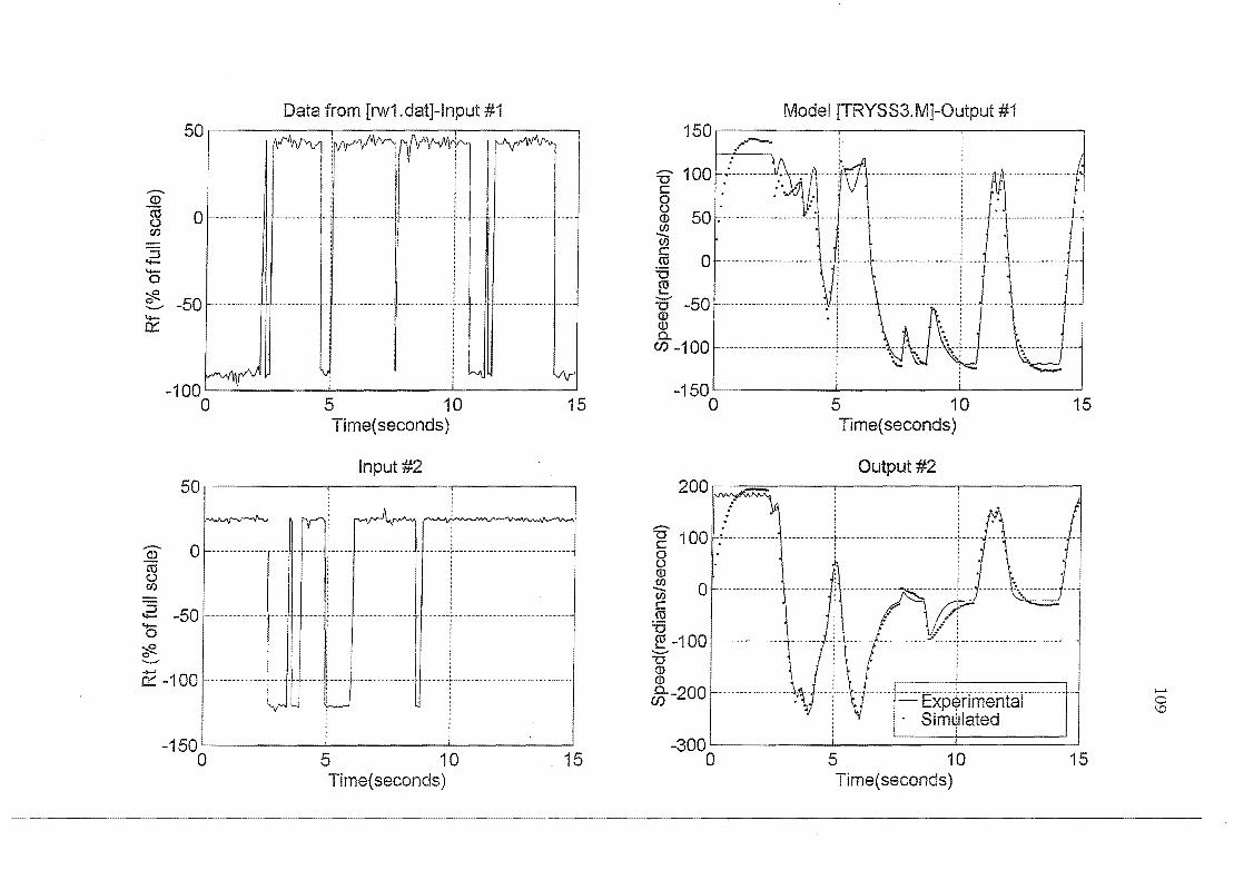
Data from [rw1.dat]-lnput #1 50
(j)
~ 0 CIJ
'6 ~ -50 (E
-100~1 --------~----------~--------~ o 5 10 15 Time( seconds)
Input #2 50~1 ----------~--------~--------~
-- 0 ~ --- ---- -~-----~--~-- -(l)
ro (.) CIJ
:::J 4- -50 -------------4-0
~ 0
----C2 -100
-150~i --------~----------~------~ o 5 10 15 Time( seconds)
Model [TRYSS3.M]-Output #1 150" ---------.---------,---------,
. U 100 . c o
.. ---.'
as 50 f;----------.---------O:-~ C/)
<n c .~ 0 "'0 ~ :0- -50 (l) (l) Q..
C/) -1 00 1----------------------------~-----------1,.
-150 o 5 10
Time( seconds)
Output #2
15
200 1.i ~~----~--------.-------~
f 100F 0 u (l) C/)
0 -C/)
C co n ~ -100
'--" "'0 (l) (l)
Q..-200 C/) . :-j"-----1-·--=-Exp$rfmentar----------
Sim~lated -300 L-i ____ --'-____ -...L ____ -----'
o 5 10 15 Time( seconds)
....... o \.0
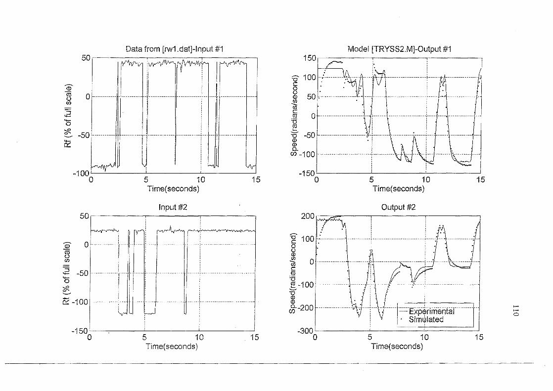
Data from [rw1.dat]-lnput #1 Model [TRYSS2.M]-Output #1 50,- -----.,--------,--------, 150 -- - 1
'iJ 100 ,(-= .,. ....c~~--····-··-----·fJ c . . :.
§ 50 .:'.'. . ... ...... L: ................ J en • , - : en : C : co 0 ··-·-·-·-------·---·~···-i----~' ~ : co i ~ , :g -50 ----·----·-f\-~-·----r-··-}--·-·-}--------··-1-(J) • :
c% -1 00 -A.-- ." +··I·---···-\"~:·"-····-··
ill ro 0 I-··---------H+---------++---------··-o (J)
.2
;:R ~ -50 ~----- .. ----0:::
-100' -150 0 5 10 15 0 5 10 15
Time(seconds) Time( seconds)
Input #2 Output #2 50 200
1 rvv~ •..•
- 0 ----~-. ----~~-------
~ 100 : CD 0 co ()
0 (J) U) en
0 -en -50
c ------~~~---- co
"I- :0 0 ~ -100 ?f2. I '-" --- ""0
C2 -100 .. - -~ (J) - -.. -- - _ .. ~ ---- (J)
c% -200 I---""-·---· .. -----ttt~j---·r--tj ------j:=-Exp$rfmenfal·--------t-1 I-' I-' 0
. Sim~lated I -_ ....•.
-150 l. -300 0 5 10 15 0 5 10 15
Time(seconds) Time( seconds)
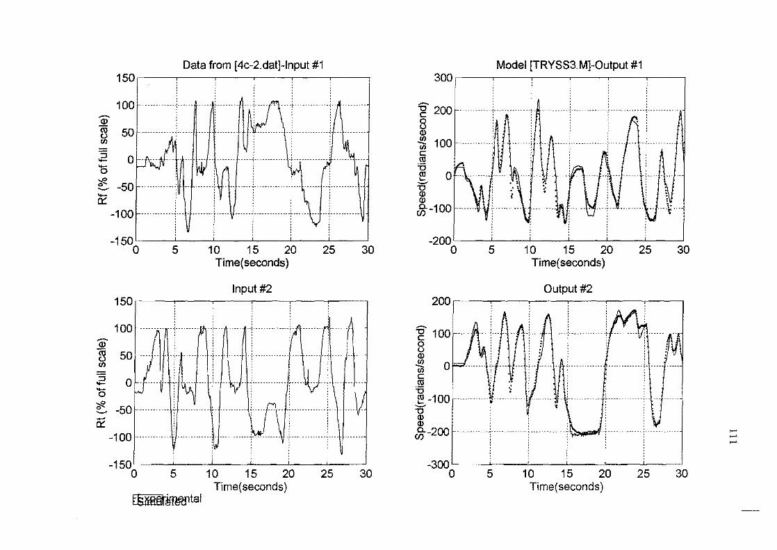
Data from [4c-2.dat]-lnput #1 150r----~--~--~----~--~--~
100 -Q)
~ 50 (I)
'0 o ~ -50 - ••••• ~----- ... I- .. -- •• ------- _ ....... -_
CE -100 .. _4 .. _ ~ ______ .... __ J .. ~ ........ ___ .. .. ...... ..
-150~' ----~--~----~--~----~--~ o 5 10 15 20 25 30 Time( seconds)
Input #2 150~, ----~--~----~--~--~----~
-Q)
r3 (I)
.2 0 '0 ~ -50 a::
-100
-150~' ----~--~----~--~----~--~ o 5 10 15 20 25 30 Time(seconds)
f§rre§r~tal
Model [TRYSS3.M]-Output #1 300,~--~----~--~----~--~----.
13' c 8 Q) tf) -tf) C aJ U ~ 0 -"0 Q) Q)
c%-100
, , , __________ .J ______________ 1.. _____________ ..I ___________ _ . . . : : n: : ; . : , , , , , , , , , , , ,
-·---··-.. --i---------· .. --:------- .-- --1----------_·-
-200'~--~----~--~----~--~--~
o 5 10 15 20 25 30 Time( seconds)
Output #2 200 1, ---:----~--~--~----~--~
-"0 100 c 8 Q)
..ce 0 tf) C aJ U ~ -100 :0-Q) Q)
c%-200
-300~' __ ----I. ___ ..L-_--L...._---..J __ --1-__ _
o 5 10 15 20 25 30 Time(seconds)
......
......
......
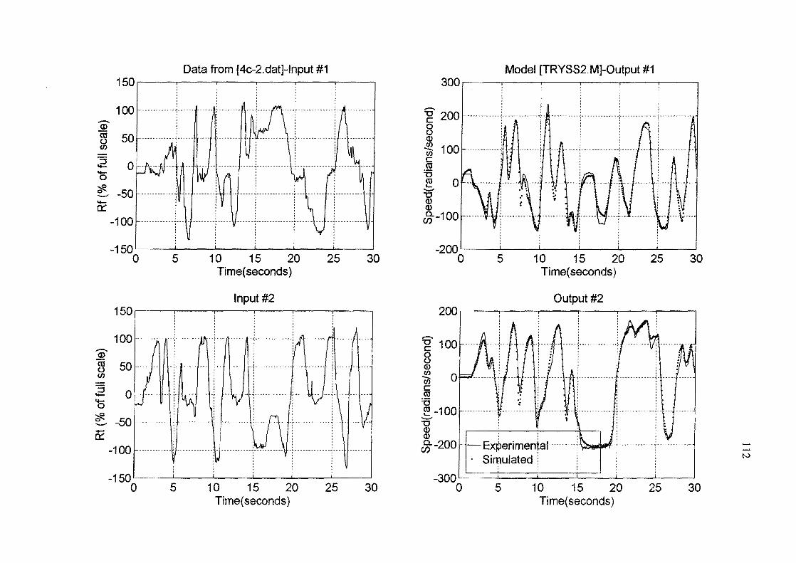
Data from [4c-2.dat]-lnput #1 150~1 ----~--~----~--~----~---.
100 -Q)
~ 50 (/)
.2 0 '0 ~ -50 ~
-100
-150 '---'-----'----'--------'-----1.-----'
o 5 10 15 20 25 30 Time( seconds)
Input #2 150~, ---~-~---~-~---~--.
100 <D ~ 50 en ::; -'0 ~ -50 li
-100
-150' o 5 10 15 20 25 30
Time( seconds)
Model [TRYSS2.M]-Output #1 300~1 ----~-~----~-~---~-~
:c c: 8 ~ c: ro =a ~ --g (I)
&--100
~OO~I ----~-~--~-~--~--~ o 5 10 15 20 25 30 Time( seconds)
Output #2 200,---...,.-----,------,--------r----r----,
~ 100 8 (I)
~ c: ro 15 ~ -100 ........
"0 (I) (I)
&--200 . ,
- Ex~ertmental----------~-~Si~ulated i
-300 ~==:1====t::===::t==_.....L....._-L_~ o 5 10 15 20 25 30
Time( seconds)
..... ..... N
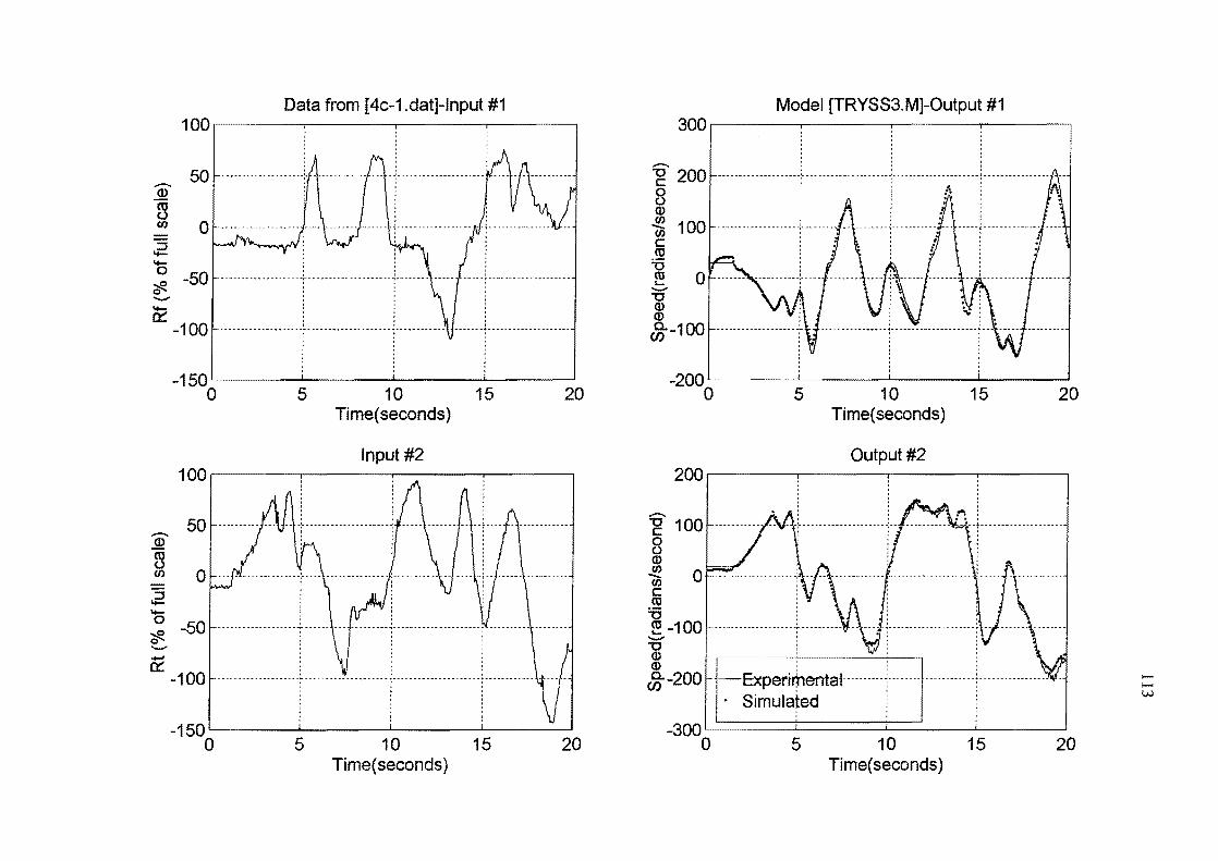
Data from [4c-1.dat]-lnput #1 100,~----~------~------~-------.
CD ro
50
~ 0
-o -50 ~ o .......... -0::: -100
-150~1 ------~------~------~----~ o 5 10 15 20
Time( seconds)
Input #2 100~j ------~------~------------~---------.
50 .-(J)
~ 0 .2 -o -50 ~ o .......... ...... 0::: -100
-150~1 ------~------~------~----~ o 5 10 15 20 Time( seconds)
Model [TRYSS3. M]-Output #1 300~j ------~------~------~------.
:g 200 8 (J)
~ 100 c ro
=u ~ 0 .......... "0 Q) Q)
c%-100
-200 o 5 10 15 20 Time( seconds)
Output #2 200~1 ------~----~------~----~
:s c 8 Q)
.!e 0 UJ c ro
=u ~ -100 '-" "0 Q) Q)
c%-200
-300 o
-Experimental· .. ··············· Simulated
5 10 15 Time( seconds)
20
........
........ w
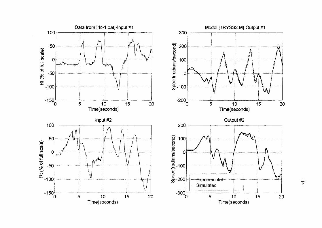
Data from [4c-1.dat]-lnput #1 100 r-----r------,-------.,------,
50 ...-.. <l>
~ (/) 0 ::J -'0 -50 :::R 0 ........ -0::: -100
-<l>
rl (/)
.2 -
-150 .. o
100
50
o -50 :::R o '-'" .......
0::: -100
5 10 15 20 Time(seconds)
Input #2
-150~' ------~------~----~------~ o 5 10 15 20 Time( seconds)
......... "'0 c: 8 Q)
~ c: ro U
300
~ 0 ........ "'0 Q) Q)
~-100
Model [TRYSS2. M]-Output #1
~oo~' ______ ~ ____ -L ______ L-____ _
o 5 10 15 20 Time( seconds)
Output #2 200, --------,------.----.,----~
~ 100 8 Q)
.!!? 0 w c: ro U ~ -100 ........
"'0 Q) Q)
~-200
, ,
-·-Experifttenta~--· .. ·-··~--····--Simul~ed i
-300 1 '---. o -~===::::±~ 5 10 15
Time( seconds) 20
>-' >-' .j:>.