Embed Size (px)
Citation preview
Ideas on Updating Model Evaluation Methods
byJohn S. Irwin
EPA Eight Conference on Air Quality ModelingSeptember 22-23, 2005
US Environmental Protection Agency, RTP, NC 27711
Where Are We Now
• EPA has defined the Cox/Tikvart methodology. The BOOT program (developed by Chang and Hanna) implements this procedure. EPA once started to develop software for this, but it never got finalized.
• Most recently, AERMIC has employed various test data sets. The intensive tracer experiment included: Project Prairie Grass, EPRI Kinciad, EPRI Indianapolis. There are of order ten non-intensive data sets that have also been used. I think EPA would be willing to provide all these data if called upon to do so..
• EPA defined a model evaluation procedure, and this does provide a means for ranking skill, but I do not think it provides a means for defining whether differences in skill are significant.
• The current evaluation methods in use do not account for the fact that air quality transport and diffusion involves stochastic processes that preclude simulation of exactly what is seen. You may want to predict exactly where the transport will be, but it is only possible “on average.” More on this later.
What Might Be Changed?• Can we move the process to include more experts to help in devising, testing, drafting and
promulgating model performance test methods, test data sets, testing software? The short answer is yes. This is the purpose of voluntary standards development organizations (like ASTM). The more complete answer is that EPA must actively participate to insure EPA’s interests are protected.
• Test methods could be drafted within ASTM and passed as ASTM standards. This provides a new level of review and scrutiny. It also provides a basis for continual review and upgrading in the future, as ASTM requires all standards to be reapproved at least every five years.
• Having a standard committee provides a place to develop expertise for succession (retiring experts) and future continuity (“How we got here” history).
• Working within ASTM, other test methods can be devised, tested and converted to ASTM standards. This could in the future provide tests as models develop new capabilities (e.g., characterization of stochastic effects).
• Working in a collective of Federal and Private experts, we may find ways to provide test data sets more completely (e.g., co-funding by several agencies, entrepreneurial interest – software providers who provide test data as a perk to attract customers).
Common Worries
• EPA will be forced to “accept” test methods.– How? EPA will be stating what test methods will be
“acceptable” to EPA in the Model Guideline.
• EPA will lose control.– If EPA does not participate in the voluntary standards
development process, then yes, in a sense, EPA loses control. On the flip side, the reason I suggest moving the process out to a communal activity is to enlist help from others and to cultivate a standing committee of experts that will promote better test methods in the future.
What Can We Do Now?• At best, models predict the statistical properties of what is to be seen “on average”,
whereas observations are individual realizations from imperfectly known ensembles.– We need to get this message out so that it is commonplace knowledge.– We need to devise evaluation methods that account for variability in the observations that
models cannot ever explicitly simulate. You can fully explain the distribution of outcomes to occur when a pair of dice are rolled, but you will never predict the exact sequence of outcomes.
• ASTM D 6589 was recently updated and submitted for reapproval. It outlines the problem as stated above, and provides one example test procedure. The appendix of D 65898 could be converted into a Standard Practice. Who wants to participate in this?
• The Cox/Tikvart method could be drafted as a Standard Practice, but should inform users of what to expect with 1st-order dispersion models (e.g., ISC, AERMOD). Who wants to participate in this?
• There are more ideas that people have on candidate test methods, many of which could be converted to ASTM standards, but people have to volunteer their time and talents to create the envisioned “standing committee”.
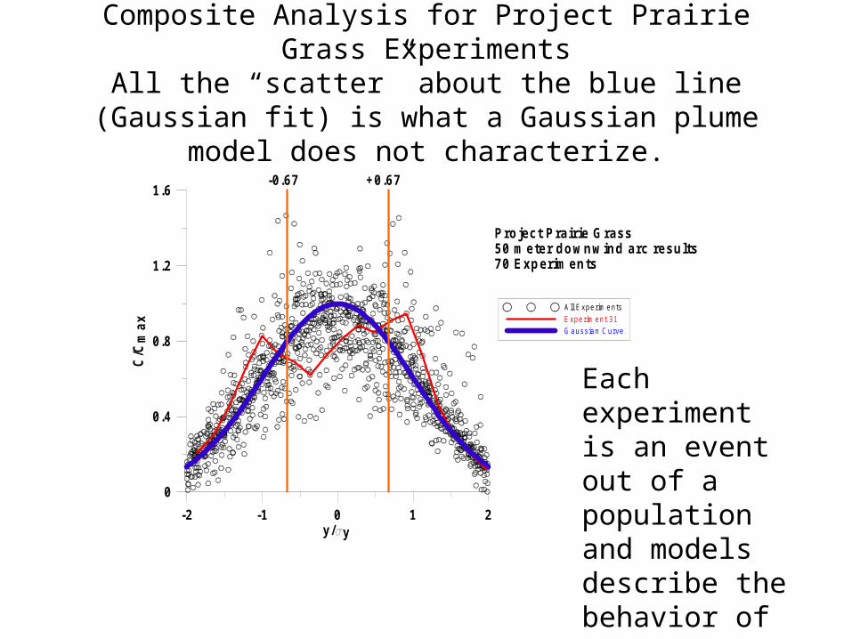
Composite Analysis for Project Prairie Grass Experiments
All the “scatter” about the blue line (Gaussian fit) is what a Gaussian plume model does not characterize.
-2 -1 0 1 2y/ y
0
0.4
0.8
1.2
1.6
C/C
max
A ll E xperim ents
E xperim ent 31
G aussian C urve
Project Prairie Grass50 meter downwind arc results70 Experiments
-0.67 +0.67
Each experiment is an event out of a population and models describe the behavior of the ensemble mean

0.01 0.10 1.00 10.00 100.00Downwind Distance (km)
1.0
1.5
2.0
2.5
3.0C
en
terl
ine
Val
ues
Geo
Std
Near-S fc (S im ple)Near-S fc (C om plex)E levated (S im ple)K incaidLovettIndianapolis
Avg = 1.77
Avg + 2Std = 2.39
Avg - 2Std = 1.15
▲1.69(0.20)
▲2.17 (0.07)
■2.00 (0.20)
▼2.00 (0.23)
●1.78 (0.35)
●1.53 (0.24)
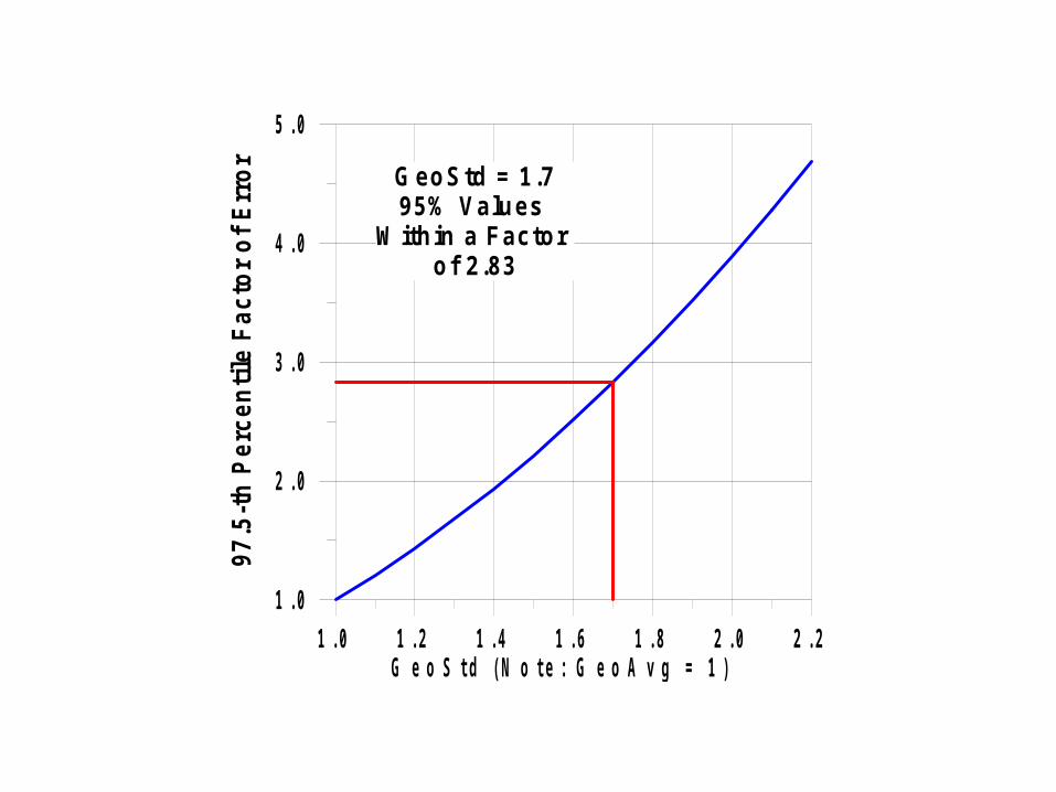
1 . 0 1 . 2 1 . 4 1 . 6 1 . 8 2 . 0 2 . 2G e o S t d ( N o t e : G e o A v g = 1 )
1 . 0
2 . 0
3 . 0
4 . 0
5 . 0
97.5
-th
Pe
rcen
tile
Fac
tor
of
Err
or
GeoStd = 1.795% Values
W ithin a Factor of 2.83
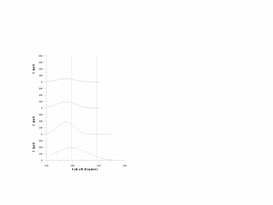
160 200 240 280
A zimuth (D egrees)
0
100
200
300
C (
pp
t)
0
100
200
300
C (
pp
t)
0
100
200
300
0
100
200
300
400
C (
pp
t)
Sy = 24.5 degreesPH IC = 198.8 degrees
5.8 km
7.5 km
9.9 km
3.8 km
Sy = 12.6 degreesPH IC = 190.1 degrees
Sy = 15.0 degreesPH IC = 190.2 degrees
Sy = 14.4 degreesPH IC = 189.7 degrees
KincaidApril 25, 19801100-1200 LST
AVGPH IC W D 100
0
100
200
300
C (
pp
t)
.Analysis of 1-hr concentration values seen for April 25, 1980 from 1200 to 1300 LST. Results are shown for four arcs.
Solid lines with symbols show measured SF6 values. A Gaussian fit is shown for each arc. The resulting plume centerline position, PHIC, and lateral dispersion, Sy, is shown for each arc.
The two vertical solid lines illustrates the transport wind direction indicated by the 100-m wind and the average of the PHIC determined individually for each arc.
The dotted line (second arc) shows the effect of differences in transport between what is estimated by a wind direction at the release and what actually occurs.
The Kincaid tracer experiments involved injecting SF6 into the gas exiting up a power-plant smoke stack. The smoke stack was 183 m tall, and the gases were hotter than the air, rose and leveled off at about 300 m above the ground.