Ideal Whitehead Graphs in Out(Fr) I: Some Unachieved Graphs

Catherine Pfaff

Abstract

In [MS93], Masur and Smillie proved precisely which singularity index lists arise from pseudo-Anosovmapping classes. In search of an analogous theorem for outer automorphisms of free groups, Handeland Mosher ask in [HM11]: Is each connected, simplicial, (2r − 1)-vertex graph the ideal Whiteheadgraph of a fully irreducible ϕ ∈ Out(Fr)? We answer this question in the negative by exhibiting, foreach r, examples of connected (2r-1)-vertex graphs that are not the ideal Whitehead graph of any fullyirreducible ϕ ∈ Out(Fr). In the course of our proof we also develop machinery used in [Pfa12] to fullyanswer the question in the rank-three case.

1 Introduction

For a compact surface S, the mapping class group MCG(S) is the group of isotopy classes of homeo-morphisms h : S → S. A generic (see, for example, [Mah11]) mapping class is pseudo-Anosov, i.e. hasa representative leaving invariant a pair of transverse measured singular minimal foliations. From thefoliation comes a singularity index list. Masur and Smillie determined precisely which singularity indexlists, permitted by the Poincare-Hopf index formula, arise from pseudo-Anosovs [MS93]. The search foran analogous theorem in the setting of an outer automorphism group of a free group is still open.

We let Out(Fr) denote the outer automorphism group of the free group of rank r. Analogous topseudo-Anosov mapping classes are fully irreducible outer automorphisms, i.e. those such that nopower leaves invariant the conjugacy class of a proper free factor. In fact, some fully irreducible outerautomorphisms, called geometrics, are induced by pseudo-Anosovs. The index lists of geometrics areunderstood through the Masur-Smillie index theorem.

In [GJLL98], Gaboriau, Jaeger, Levitt, and Lustig defined singularity indices for fully irreducibleouter automorphisms. Additionally, they proved an Out(Fr)-analogue to the Poincare-Hopf indexequality. After switching the index sign for consistency with the surface case and using a version of theindex definition invariant under taking powers, the index sum inequality is 0 ≥ i(ϕ) ≥ 1− r for a fullyirreducible ϕ ∈ Out(Fr).

Having an inequality, instead of just an equality, makes the search for an analogue to the Masur-Smillie theorem richly more complicated. Toward this goal, Handel and Mosher asked in [HM11]:

Question 1.1. Which index types, satisfying 0 ≥ i(ϕ) > 1 − r, are achieved by nongeometric fullyirreducible ϕ ∈ Out(Fr)?

There are several results on related questions. For example, [JL09] gives examples of automorphismswith the maximal number of fixed points on ∂Fr, as dictated by a related inequality in [GJLL98].

1

However, our work focuses on an Out(Fr)-version of the Masur-Smillie theorem. Hence, in this paper,in [Pfa13a], and in [Pfa13b] we restrict attention to fully irreducibles and the [GJLL98] index inequality.

Beyond the existence of an inequality, instead of just an equality, “ideal Whitehead graphs” give yetanother layer of complexity for fully irreducibles. An ideal Whitehead graph describes the structure ofsingular leaves, in analogue to the boundary curves of principle regions in Nielsen theory [NH86]. Inthe surface case, ideal Whitehead graphs are all circles. However, the ideal Whitehead graph IW(ϕ)for a fully irreducible ϕ ∈ Out(Fr) (see [HM11] or Definition 2.1 below) gives a strictly finer outerautomorphism invariant than just the corresponding index list. Indeed, each connected componentCi of IW(ϕ) contributes the index 1 − ki

2 to the list, where Ci has ki vertices. One can see manycomplicated ideal Whitehead graph examples, including complete graphs in every rank (in [Pfa13a])and in the eighteen of the twenty-one connected, five-vertex graphs achieved by fully irreducibles inrank-three ([Pfa13b]). The deeper, more appropriate question is thus:

Question 1.2. Which isomorphism types of graphs occur as the ideal Whitehead graph IW(ϕ) of afully irreducible outer automorphism ϕ?

[Pfa13b] will give a complete answer to Question 1.2 in rank 3 for the single-element index list (−32).

In Theorem 9.1 of this paper we provide examples in each rank of connected (2r-1)-vertex graphs thatare not the ideal Whitehead graph IW(ϕ) for any fully irreducible ϕ ∈ Out(Fr), i.e. that are unachievedin rank r:

Theorem. For each r ≥ 3, let Gr be the graph consisting of 2r − 2 edges adjoined at a single vertex.

A. For no fully irreducible ϕ ∈ Out(Fr) is IW(ϕ) ∼= Gr.

B. The following connected graphs are not the ideal Whitehead graph IW(ϕ) for any fully irreducibleϕ ∈ Out(F3):

Nongeometric fully irreducible outer automorphisms are either “ageometric” or “parageometric,” asdefined by Lustig. Ageometric outer automorphisms are our focus, since the index sum for a parageo-metric, as is true for a geometric, satisfies the Poincare-Hopf equality [GJLL98]. Parageometrics havebeen studied in papers including [HM07]. In [BF94], Bestvina and Feighn prove the [GJLL98] indexinequality is strict for ageometrics.

For a fully irreducible ϕ ∈ Out(Fr), to have the index list (32 − r), ϕ must be ageometric witha connected, (2r-1)-vertex ideal Whitehead graph IW(ϕ). We chose to focus on the single-elementindex list (32 − r) because it is the closest to that achieved by geometrics, without being achieved by ageometric. We denote the set of connected (2r − 1)-vertex, simplicial graphs by PI(r;( 3

2−r)).

One often studies outer automorphisms via geometric representatives. Let Rr be the r-petaled rose,with its fundamental group identified with Fr. For a finite graph Γ with no valence-one vertices, ahomotopy equivalence Rr → Γ is called a marking. Such a graph Γ, together with its marking Rr → Γ,is called a marked graph. Each ϕ ∈ Out(Fr) can be represented by a homotopy equivalence g : Γ → Γ ofa marked graph (ϕ = g∗ : π1(Γ) → π1(Γ)). Thurston defined such a homotopy equivalence to be a traintrack map when gk is locally injective on edge interiors for each k > 0. When g induces ϕ ∈ Out(Fr)and sends vertices to vertices, one says g is a train track (tt) representative for ϕ [BH92].

To prove Theorem 9.1A, we give a necessary Birecurrency Condition (Proposition 4.4) on “lamina-tion train track structures.” For a train track representative g : Γ → Γ on a marked rose, we define a

2

lamination train track (ltt) Structure G(g) obtainable from Γ by replacing the vertex v with the “localWhitehead graph” LW(g; v). The local Whitehead graph encodes how lamination leaves enter and exitv. In our circumstance, IW(ϕ) will be a subgraph of LW(g; v), hence of G(g).

The lamination train track structure G(g) is given a smooth structure so that leaves of the expandinglamination are realized as locally smoothly embedded lines. It is called birecurrent if it has a locallysmoothly embedded line crossing each edge infinitely many times as R → ∞ and as R → −∞.

Proposition. (Birecurrency Condition) The lamination train track structure for each train trackrepresentative of each fully irreducible outer automorphism ϕ ∈ Out(Fr) is birecurrent.

Combinatorial proofs (not included here) of Theorem 9.1A exist. However, we include a proofusing the Birecurrency Condition to highlight what we have observed to be a significant obstacle toachievability, namely the birecurrency of ltt structures. The Birecurrency Condition is also used inour proof of Theorem 9.1B. We use it in [Pfa13a], where we prove the achievability of the completegraph in each rank. Finally, the condition is used in [Pfa13b] to prove precisely which of the twenty-oneconnected, simplicial, five-vertex graphs are IW(ϕ) for fully irreducible ϕ ∈ Out(F3).

In Proposition 3.3 we show that each ϕ, such that IW(ϕ) ∈ PI(r;( 32−r)), has a power ϕR with

a rotationless representative whose Stallings fold decomposition (see Subsection 3.2) consists entirelyof proper full folds of roses (see Subsection 3.3). The representatives of Proposition 3.3 are called“ideally decomposable.” We define in Section 8 automata, ideal “decomposition (ID) diagrams” withltt structures as nodes. Every ideally decomposed representative is realized by a loop in an ID diagram.To prove Theorem 9.1B we show ideally decomposed representatives cannot exist by showing that theID diagrams do not have the correct kind of loops.

We again use the ideally decomposed representatives and ID diagrams in [Pfa13a] and [Pfa13b] toconstruct ideally decomposed representatives with particular ideal Whitehead graphs.

To determine the edges of the ID diagrams, we prove in Section 5 a list of “Admissible Map (AM)properties” held by ideal decompositions. In Section 7 we use the AM properties to determine the twogeometric moves one applies to ltt structures in defining edges of the ID diagrams. The geometricmoves turn out to have useful properties expanded upon in [Pfa13a] and [Pfa13b].

Acknowledgements

The author would like to thank Lee Mosher for his truly invaluable conversations and Martin Lustigfor his interest in her work. She also extends her gratitude to Bard College at Simon’s Rock and theCRM for their hospitality.

2 Preliminary definitions and notation

We continue with the introduction’s notation. Further we assume throughout this document thatall representatives g of ϕ ∈ Out(Fr) are train tracks (tts).

We let FIr denoted the subset of Out(Fr) consisting of all fully irreducible elements.

2.1. Directions and turns

In general we use the definitions from [BH92] and [BFH00] when discussing train tracks. We givefurther definitions and notation here. g : Γ → Γ will represent ϕ ∈ Out(Fr).

3

E+(Γ) = {E1, . . . , En} = {e1, e1, . . . , e2n−1, e2n} will be the edge set of Γ with some prescribedorientation. For E ∈ E+(Γ), E will be E oppositely oriented. E(Γ):= {E1, E1, . . . , En, En}. If theindexing {E1, . . . , En} of the edges (thus the indexing {e1, e1, . . . , e2n−1, e2n}) is prescribed, we call Γan edge-indexed graph. Edge-indexed graphs differing by an index-preserving homeomorphism will beconsidered equivalent.

V(Γ) will denote the vertex set of Γ (V, when Γ is clear) and D(Γ) will denote ∪v∈V(Γ)

D(v), where

D(v) is the set of directions (germs of initial edge segments) at v.For each e ∈ E(Γ), D0(e) will denote the initial direction of e and D0γ := D0(e1) for each path

γ = e1 . . . ek in Γ. Dg will denote the direction map induced by g. We call d ∈ D(Γ) periodic ifDgk(d) = d for some k > 0 and fixed if k = 1.

Per(x) will consist of the periodic directions at an x ∈ Γ and Fix(x) of those fixed. Fix(g) willdenote the fixed point set for g.

T (v) will denote the set of turns (unordered pairs of directions) at a v ∈ V(Γ) and Dtg the inducedmap of turns. For a path γ = e1e2 . . . ek−1ek in Γ, we say γ contains (or crosses over) the turn {ei, ei+1}for each 1 ≤ i < k. Sometimes we abusively write {ei, ej} for {D0(ei), D0(ej)}. Recall that a turn iscalled illegal for g if Dgk(di) = Dgk(dj) for some k (di and dj are in the same gate).

2.2. Periodic Nielsen paths and ageometric outer automorphisms

Recall [BF94] that a periodic Nielsen path (pNp) is a nontrivial path ρ between x, y ∈ Fix(g) suchthat, for some k, gk(ρ) ≃ ρ rel endpoints (Nielsen path (Np) if k = 1). In later sections we use[GJLL98] that a ϕ ∈ FIr is ageometric if and only if some ϕk has a representative with no pNps (closedor otherwise). AFIr will denote the subset of FIr consisting precisely of its ageometric elements.

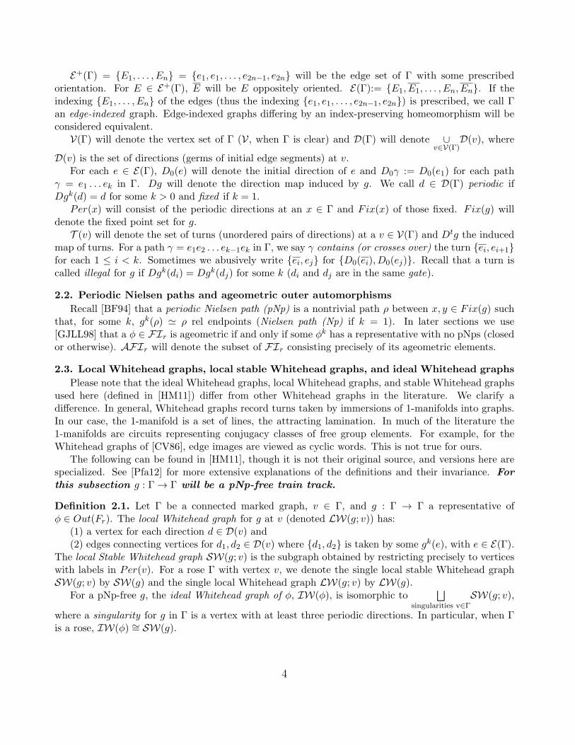
2.3. Local Whitehead graphs, local stable Whitehead graphs, and ideal Whitehead graphs

Please note that the ideal Whitehead graphs, local Whitehead graphs, and stable Whitehead graphsused here (defined in [HM11]) differ from other Whitehead graphs in the literature. We clarify adifference. In general, Whitehead graphs record turns taken by immersions of 1-manifolds into graphs.In our case, the 1-manifold is a set of lines, the attracting lamination. In much of the literature the1-manifolds are circuits representing conjugacy classes of free group elements. For example, for theWhitehead graphs of [CV86], edge images are viewed as cyclic words. This is not true for ours.

The following can be found in [HM11], though it is not their original source, and versions here arespecialized. See [Pfa12] for more extensive explanations of the definitions and their invariance. Forthis subsection g : Γ → Γ will be a pNp-free train track.

Definition 2.1. Let Γ be a connected marked graph, v ∈ Γ, and g : Γ → Γ a representative ofϕ ∈ Out(Fr). The local Whitehead graph for g at v (denoted LW(g; v)) has:

(1) a vertex for each direction d ∈ D(v) and(2) edges connecting vertices for d1, d2 ∈ D(v) where {d1, d2} is taken by some gk(e), with e ∈ E(Γ).

The local Stable Whitehead graph SW(g; v) is the subgraph obtained by restricting precisely to verticeswith labels in Per(v). For a rose Γ with vertex v, we denote the single local stable Whitehead graphSW(g; v) by SW(g) and the single local Whitehead graph LW(g; v) by LW(g).

For a pNp-free g, the ideal Whitehead graph of ϕ, IW(ϕ), is isomorphic to⊔

singularities v∈ΓSW(g; v),

where a singularity for g in Γ is a vertex with at least three periodic directions. In particular, when Γis a rose, IW(ϕ) ∼= SW(g).

4

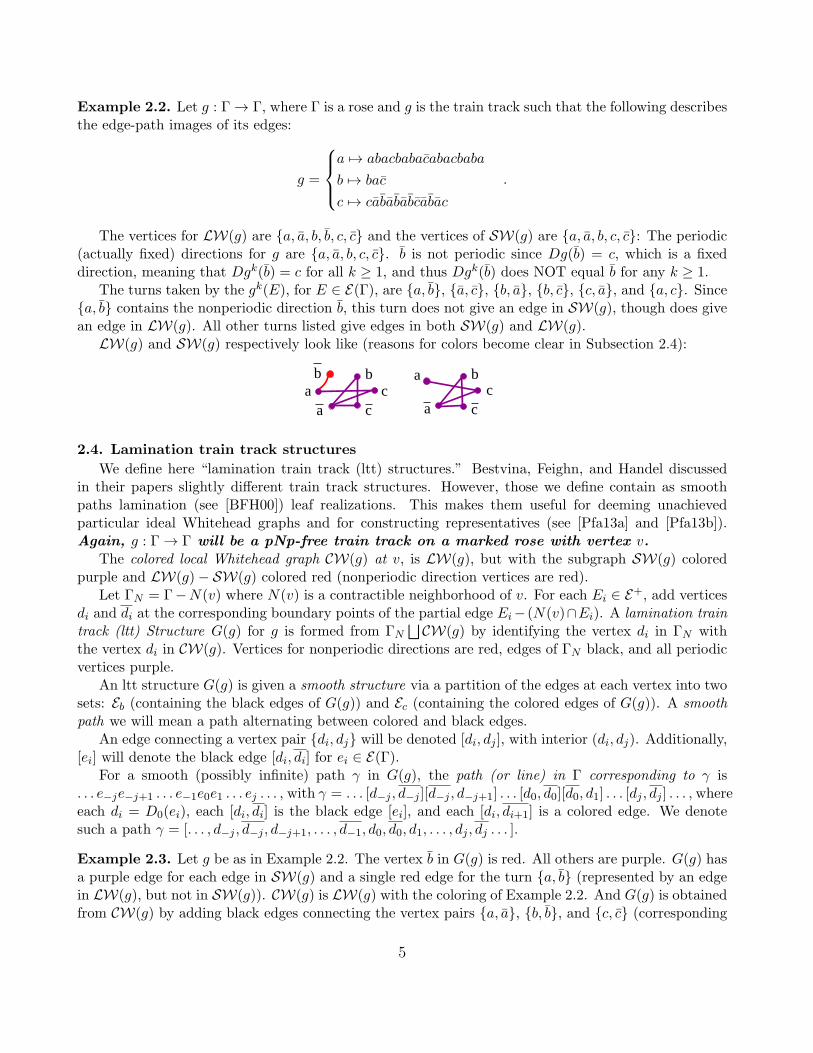
Example 2.2. Let g : Γ → Γ, where Γ is a rose and g is the train track such that the following describesthe edge-path images of its edges:

g =

a 7→ abacbabacabacbaba

b 7→ bac

c 7→ cabababcabac

.

The vertices for LW(g) are {a, a, b, b, c, c} and the vertices of SW(g) are {a, a, b, c, c}: The periodic(actually fixed) directions for g are {a, a, b, c, c}. b is not periodic since Dg(b) = c, which is a fixeddirection, meaning that Dgk(b) = c for all k ≥ 1, and thus Dgk(b) does NOT equal b for any k ≥ 1.

The turns taken by the gk(E), for E ∈ E(Γ), are {a, b}, {a, c}, {b, a}, {b, c}, {c, a}, and {a, c}. Since{a, b} contains the nonperiodic direction b, this turn does not give an edge in SW(g), though does givean edge in LW(g). All other turns listed give edges in both SW(g) and LW(g).

LW(g) and SW(g) respectively look like (reasons for colors become clear in Subsection 2.4):

ba c

bac

b

a c ca

2.4. Lamination train track structures

We define here “lamination train track (ltt) structures.” Bestvina, Feighn, and Handel discussedin their papers slightly different train track structures. However, those we define contain as smoothpaths lamination (see [BFH00]) leaf realizations. This makes them useful for deeming unachievedparticular ideal Whitehead graphs and for constructing representatives (see [Pfa13a] and [Pfa13b]).Again, g : Γ → Γ will be a pNp-free train track on a marked rose with vertex v.

The colored local Whitehead graph CW(g) at v, is LW(g), but with the subgraph SW(g) coloredpurple and LW(g)− SW(g) colored red (nonperiodic direction vertices are red).

Let ΓN = Γ−N(v) where N(v) is a contractible neighborhood of v. For each Ei ∈ E+, add verticesdi and di at the corresponding boundary points of the partial edge Ei− (N(v)∩Ei). A lamination traintrack (ltt) Structure G(g) for g is formed from ΓN

⊔CW(g) by identifying the vertex di in ΓN with

the vertex di in CW(g). Vertices for nonperiodic directions are red, edges of ΓN black, and all periodicvertices purple.

An ltt structure G(g) is given a smooth structure via a partition of the edges at each vertex into twosets: Eb (containing the black edges of G(g)) and Ec (containing the colored edges of G(g)). A smoothpath we will mean a path alternating between colored and black edges.

An edge connecting a vertex pair {di, dj} will be denoted [di, dj ], with interior (di, dj). Additionally,[ei] will denote the black edge [di, di] for ei ∈ E(Γ).

For a smooth (possibly infinite) path γ in G(g), the path (or line) in Γ corresponding to γ is. . . e−je−j+1 . . . e−1e0e1 . . . ej . . . , with γ = . . . [d−j , d−j ][d−j , d−j+1] . . . [d0, d0][d0, d1] . . . [dj , dj ] . . . , whereeach di = D0(ei), each [di, di] is the black edge [ei], and each [di, di+1] is a colored edge. We denotesuch a path γ = [. . . , d−j , d−j , d−j+1, . . . , d−1, d0, d0, d1, . . . , dj , dj . . . ].

Example 2.3. Let g be as in Example 2.2. The vertex b in G(g) is red. All others are purple. G(g) hasa purple edge for each edge in SW(g) and a single red edge for the turn {a, b} (represented by an edgein LW(g), but not in SW(g)). CW(g) is LW(g) with the coloring of Example 2.2. And G(g) is obtainedfrom CW(g) by adding black edges connecting the vertex pairs {a, a}, {b, b}, and {c, c} (corresponding

5

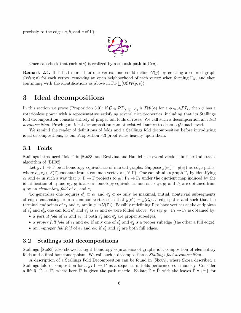
precisely to the edges a, b, and c of Γ).

ba c

b

a c

Once can check that each g(e) is realized by a smooth path in G(g).

Remark 2.4. If Γ had more than one vertex, one could define G(g) by creating a colored graphCW(g; v) for each vertex, removing an open neighborhood of each vertex when forming ΓN , and thencontinuing with the identifications as above in ΓN

⊔(∪CW(g; v)).

3 Ideal decompositions

In this section we prove (Proposition 3.3): if G ∈ PI(r;( 32−r)) is IW(ϕ) for a ϕ ∈ AFIr, then ϕ has a

rotationless power with a representative satisfying several nice properties, including that its Stallingsfold decomposition consists entirely of proper full folds of roses. We call such a decomposition an idealdecomposition. Proving an ideal decomposition cannot exist will suffice to deem a G unachieved.

We remind the reader of definitions of folds and a Stallings fold decomposition before introducingideal decompositions, as our Proposition 3.3 proof relies heavily upon them.

3.1 Folds

Stallings introduced “folds” in [Sta83] and Bestvina and Handel use several versions in their train trackalgorithm of [BH92].

Let g : Γ → Γ be a homotopy equivalence of marked graphs. Suppose g(e1) = g(e2) as edge paths,where e1, e2 ∈ E(Γ) emanate from a common vertex v ∈ V(Γ). One can obtain a graph Γ1 by identifyinge1 and e2 in such a way that g : Γ → Γ projects to g1 : Γ1 → Γ1 under the quotient map induced by theidentification of e1 and e2. g1 is also a homotopy equivalence and one says g1 and Γ1 are obtained fromg by an elementary fold of e1 and e2.

To generalize one requires e′1 ⊂ e1 and e′2 ⊂ e2 only be maximal, initial, nontrivial subsegmentsof edges emanating from a common vertex such that g(e′1) = g(e′2) as edge paths and such that theterminal endpoints of e1 and e2 are in g

−1(V(Γ)). Possibly redefining Γ to have vertices at the endpointsof e′1 and e′2, one can fold e′1 and e′2 as e1 and e2 were folded above. We say g1 : Γ1 → Γ1 is obtained by

• a partial fold of e1 and e2: if both e′1 and e′2 are proper subedges;

• a proper full fold of e1 and e2: if only one of e′1 and e′2 is a proper subedge (the other a full edge);

• an improper full fold of e1 and e2: if e′1 and e′2 are both full edges.

3.2 Stallings fold decompositions

Stallings [Sta83] also showed a tight homotopy equivalence of graphs is a composition of elementaryfolds and a final homeomorphism. We call such a decomposition a Stallings fold decomposition.

A description of a Stallings Fold Decomposition can be found in [Sko89], where Skora described aStallings fold decomposition for a g : Γ → Γ′ as a sequence of folds performed continuously. Considera lift g : Γ → Γ′, where here Γ′ is given the path metric. Foliate Γ x Γ′ with the leaves Γ x {x′} for

6

x′ ∈ Γ′. Define Nt(g) = {(x, x′) ∈ Γ x Γ′ | d(g(x), x′) ≤ t}. For each t, by restricting the foliation to Nt

and collapsing all leaf components, one obtains a tree Γt. Quotienting by the Fr-action, one sees thesequence of folds performed on the graphs below over time.

Alternatively, at an illegal turn for g : Γ → Γ, fold maximal initial segments having the same imagein Γ′ to obtain a map g1 : Γ1 → Γ′ of the quotient graph Γ1. Repeat for g

1. If some gk has no illegal turn,it will be a homeomorphism and the fold sequence is complete. Using this description, we can assumeonly the final element of the decomposition is a homeomorphism. Thus, a Stallings fold decomposition

of g : Γ → Γ can be written Γ0g1−→ Γ1

g2−→ · · · gn−1−−−→ Γn−1gn−→ Γn where each gk, with 1 ≤ k ≤ n− 1, is a

fold and gn is a homeomorphism.

3.3 Ideal Decompositions

In this subsection we prove Proposition 3.3. For the proof, we need [HM11]: For ϕ ∈ AFIr such thatIW(ϕ) ∈ PI(r;( 3

2−r)), ϕ is rotationless if and only if the vertices of IW(ϕ) are fixed by the action of

ϕ. We also need that a representative g of ϕ ∈ Out(Fr) is rotationless if and only if ϕ is rotationless.Finally, we need the following lemmas.

Lemma 3.1. Let g : Γ → Γ be a pNp-free tt representative of ϕ ∈ FIr and Γ = Γ0g1−→ Γ1

g2−→ · · · gn−1−−−→Γn−1

gn−→ Γn = Γ a decomposition of g into homotopy equivalences of marked graphs with no valence-

one vertices. Then the composition h : Γkgk+1−−−→ Γk+1

gk+2−−−→ · · · gk−1−−−→ Γk−1gk−→ Γk is also a pNp-free tt

representative of ϕ (in particular, IW(h) ∼= IW(g)).

Proof. Suppose h had a pNp ρ and hp(ρ) ≃ ρ rel endpoints. Let ρ1 = gn◦· · ·◦gk+1(ρ). If ρ1 were trivial,hp(ρ) = (gk ◦ · · · ◦ g1 ◦ gp−1)(gn ◦ · · · ◦ gk+1(ρ)) = (gk ◦ · · · ◦ g1 ◦ gp−1)(ρ1) would be trivial, contradictingρ being a pNp. So assume ρ1 is not trivial.

gp(ρ1) = gp((gk ◦ · · · ◦ g1)(ρ)) = (gn ◦ · · · ◦ gk+1) ◦ hp(ρ). Now, hp(ρ) ≃ ρ rel endpoints and so(gn ◦ · · · ◦ gk+1) ◦ hp(ρ) ≃ (gn ◦ · · · ◦ gk+1)(ρ) rel endpoints. So gp(ρ1) = gp((gk ◦ · · · ◦ g1)(ρ)) =(gn ◦ · · · ◦ gk+1) ◦ hp(ρ) is homotopic to (gn ◦ · · · ◦ gk+1)(ρ) = ρ1 rel endpoints. This makes ρ1 a pNp forg, contradicting that g is pNp-free. Thus, h is pNp-free.

Let π : Rr → Γ mark Γ1. Since g1 is a homotopy equivalence, g1 ◦ π gives a marking on Γ. So g andh differ by a change of marking and thus represent the same outer automorphism ϕ.

Finally, we show h is a train track. For contradiction’s sake suppose h(e) crossed an illegal turn{d1, d2}. Since each gj is necessarily surjective, some (gk ◦ · · · ◦ g1)(ei) would traverse e. So (gk ◦· · · ◦ g1)(ei) would cross {d1, d2}. And g2(ei) = (gn ◦ · · · ◦ gk+1) ◦ h ◦ (gk ◦ · · · ◦ g1)(ei) would cross{D(gn ◦ · · · ◦gk+1)(d1), D(gn ◦ · · · ◦gk+1)(d2)}, which would either be illegal or degenerate (since {d1, d2}is an illegal turn). This would contradict that g is a tt. So h is a tt.

Lemma 3.2. Let g : Γ → Γ be a pNp-free tt representative of ϕ ∈ FIr with 2r − 1 fixed directions and

Stallings fold decomposition Γ0g1−→ Γ1

g2−→ · · · gn−1−−−→ Γn−1gn−→ Γn. Let gi be such that g = gi ◦ gi ◦ · · · ◦ g1.

Let d(1,1), . . . , d(1,2r−1) be the fixed directions for Dg and let dj,k = D(gj◦· · ·◦g1)(d1,k) for each 1 ≤ j ≤ nand 1 ≤ k ≤ 2r − 1. Then D(gi) is injective on {d(i,1), . . . , d(i,2r−1)}.

Proof. Let d(1,1), . . . , d(1,2r−1) be the fixed directions forDf . IfD(gi) identified any of d(i,1), . . . , d(i,2r−1),then Df would have fewer than 2r-1 directions in its image.

7

Proposition 3.3. Let ϕ ∈ Out(Fr) be an ageometric, fully irreducible outer automorphism whoseideal Whitehead graph IW(ϕ) is a connected, (2r-1)-vertex graph. Then there exists a train trackrepresentative of a power ψ = ϕR of ϕ that is:

1. on the rose,2. rotationless,3. pNp-free, and4. decomposable as a sequence of proper full folds of roses.

In fact, it decomposes as Γ = Γ0g1−→ Γ1

g2−→ · · · gn−1−−−→ Γn−1gn−→ Γn = Γ, where:

(I) the index set {1, . . . , n} is viewed as the set Z/nZ with its natural cyclic ordering;(II) each Γk is an edge-indexed rose with an indexing {e(k,1), e(k,2), . . . , e(k,2r−1), e(k,2r)} where:

(a) one can edge-index Γ with E(Γ) = {e1, e2, . . . , e2r−1, e2r} such that, for each t with 1 ≤ t ≤ 2r,g(et) = ei1 . . . eis where (gn ◦ · · · ◦ g1)(e0,t) = en,i1 . . . en,is;

(b) for some ik, jk with ek,ik = (ek,jk)±1

gk(ek−1,t) :=

{ek,tek,jk for t = ik

ek,t for all ek−1,t = e±1k−1,jk

; and

(the edge index permutation for the homeomorphism in the decomposition is trivial, so left out)

(c) for each et ∈ E(Γ) such that t = jn, we have Dh(dt) = dt, where dt = D0(et).

Proof. Since ϕ ∈ AFIr, there exists a pNp-free tt representative g of a power of ϕ. Let h = gk : Γ → Γbe rotationless. Then h is also a pNp-free tt representative of some ϕR and h (and all powers of h)satisfy (2)-(3). Since h has no pNps (meaning IW(ϕR) ∼=

⊔singularities v∈Γ

SW(h; v) and, if Γ is the rose,

SW(h) ∼= IW(ϕR) ), since h fixes all its periodic directions, and since IW(ϕ) (hence IW(ϕR)) is inPI(r;( 3

2−r)), Γ must have a vertex with 2r − 1 fixed directions. Thus, Γ must be one of:

va

v

w at

v

b cdw

A1 A A2 3

b1 bb1 b

a1 a

r-1r-1

r-2

If Γ = A1, h satisfies (3). We show, in this case, we also have the decomposition for (4). However,first we show Γ cannot be A2 or A3 by ruling out all possibilities for folds in h’s Stallings decomposition.

If Γ = A2, v has to be the vertex with 2r-1 fixed directions. h has an illegal turn unless it it is ahomeomorphism, contradicting irreducibility. Note w could not be mapped to v in a way not forcingan illegal turn at w, as this would force either an illegal turn at v (if t were wrapped around some bi)or we would have backtracking on t. Because all 2r-1 directions at v are fixed by h, if h had an illegalturn, it would have to occur at w (no two fixed directions can share a gate).

The turns at w are {a, a}, {a, t}, and {a, t}. By symmetry we only need to rule out illegal turns at{a, a} and {a, t}.

First, suppose {a, a} were illegal and the first fold in the Stallings decomposition. Fold {a, a}maximally to obtain (A2)1. Completely collapsing a would change the homotopy type of A2.

8

v

w

a

t

v

wt

w’ w’

v

a

A

b1 b

a1

2

a1 (A )2 1

t1

b1 b

bb1 r-1

2

Fold

r-1

r-1

Figure 1: a1 is the portion of a not folded, a2 is the edge created by the fold, w′ is the

vertex created by the fold, and t1 is a2 ∪ t without the (now unnecessary) vertex w

Let h1 : (A2)1 → (A2)1 be the induced map of [BH92]. Since the fold of {a, a} was maximal, {a1, a1}must be legal. Since h was a train track, {t1, a1} and {t1, a1} would also be legal. But then h1 wouldfix all directions at both vertices of Γ1 (since it still would need to fix all directions at v). This wouldmake h1 a homeomorphism, again contradicting irreducibility. So {a, a} could not have been the firstturn folded. We are left to rule out {a, t}.

Suppose the first turn folded in the Stallings decomposition were {a, t}. Fold {a, t} maximally toobtain (A2)

′1. Let h

′1 : (A2)

′1 → (A2)

′1 be the induced map of [BH92]. Either

A. all of t was folded with a full power of a;B. all of t was folded with a partial power of a; orC. part of t was folded with either a full or partial power of a.

If (A) or (B) held, (A2)′1 would be a rose and h′1 would give a representative on the rose, returning

us to the case of A1. So we just need to analyze (C).Consider first (C), i.e. suppose that part of t is folded with either a full or partial power of a:

v

w

v

w

w’tFold

w’

a

ta

b1 b

2

(A )2 1

b1 b

(A )2 1’

2t 2

a2a3

r-1

or w=w’

v

a

b1 b

t2

r-1 r-1

Figure 2: Of the two scenarios on the right, the leftmost is where the fold ends in the

middle of a. a2 is a possible portion of a folded with the portion of t, a3 would be the

portion of a not folded with t, and t2 would be the portion of t not folded with a

If h = h1◦g1, where g1 is the single fold performed thus far, then h1 could not identify any directionsat w′: identifying a2 and t2 would lead to h back-tracking on t; identifying t2 and a would lead to h back-tracking on a; and h1 could not identify t2 and a3 because the fold was maximal. But then all directionsof (A2)

′1 would be fixed by h1, making h1 a homeomorphism and the decomposition complete. However,

this would make h consist of the single fold g1 and a homeomorphism, contradicting h’s irreducibility.Thus, all cases where Γ = A2 are either impossible or yield the representative on the rose for (1).

Now assume Γ = A3. v must have 2r−1 fixed directions. As with A2, since h must fix all directionsat v, if h had an illegal turn (which it still has to) it would be at w. Without losing generality assume{b, d} is an illegal turn and that the first Stallings fold maximally folds {b, d}. Folding all of b and dwould change the homotopy type. So assume (again without generality loss) either:

• all of b is folded with part of d or

• only proper initial segments of b and d are folded with each other.

9

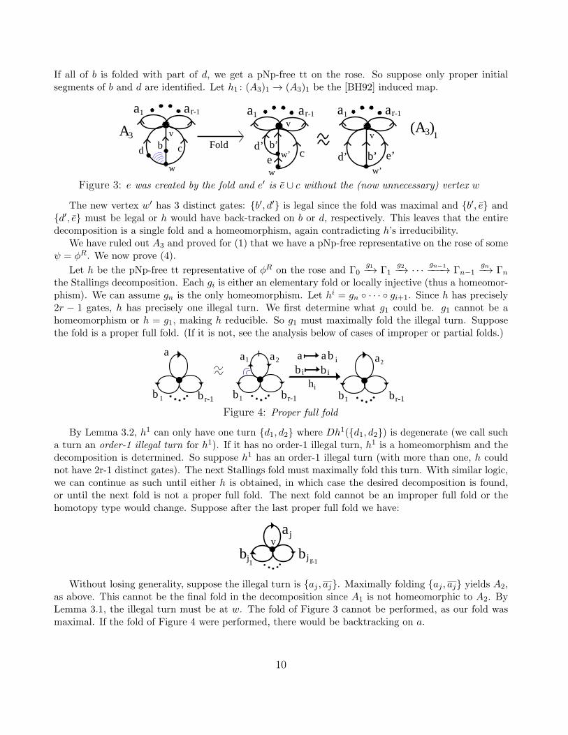
If all of b is folded with part of d, we get a pNp-free tt on the rose. So suppose only proper initialsegments of b and d are identified. Let h1 : (A3)1 → (A3)1 be the [BH92] induced map.

������

������

����

��������

���

���

������������

����

���

���

������������

����

������

������

������������

����

���

���

vb cd

v

cd’ b’

ew

w’

w

Foldd’ b’ e’

w’

v

a1 ar-1 a1 a1ar-1 ar-1

A3(A )3 1

Figure 3: e was created by the fold and e′ is e ∪ c without the (now unnecessary) vertex w

The new vertex w′ has 3 distinct gates: {b′, d′} is legal since the fold was maximal and {b′, e} and{d′, e} must be legal or h would have back-tracked on b or d, respectively. This leaves that the entiredecomposition is a single fold and a homeomorphism, again contradicting h’s irreducibility.

We have ruled out A3 and proved for (1) that we have a pNp-free representative on the rose of someψ = ϕR. We now prove (4).

Let h be the pNp-free tt representative of ϕR on the rose and Γ0g1−→ Γ1

g2−→ · · · gn−1−−−→ Γn−1gn−→ Γn

the Stallings decomposition. Each gi is either an elementary fold or locally injective (thus a homeomor-phism). We can assume gn is the only homeomorphism. Let hi = gn ◦ · · · ◦ gi+1. Since h has precisely2r − 1 gates, h has precisely one illegal turn. We first determine what g1 could be. g1 cannot be ahomeomorphism or h = g1, making h reducible. So g1 must maximally fold the illegal turn. Supposethe fold is a proper full fold. (If it is not, see the analysis below of cases of improper or partial folds.)

a a

b 1 b r-1

a1 2

b1 br-1

a2

hi

b i b i

a a b i

b1 br-1

Figure 4: Proper full fold

By Lemma 3.2, h1 can only have one turn {d1, d2} where Dh1({d1, d2}) is degenerate (we call sucha turn an order-1 illegal turn for h1). If it has no order-1 illegal turn, h1 is a homeomorphism and thedecomposition is determined. So suppose h1 has an order-1 illegal turn (with more than one, h couldnot have 2r-1 distinct gates). The next Stallings fold must maximally fold this turn. With similar logic,we can continue as such until either h is obtained, in which case the desired decomposition is found,or until the next fold is not a proper full fold. The next fold cannot be an improper full fold or thehomotopy type would change. Suppose after the last proper full fold we have:

va

b1

br-1j

j

j

Without losing generality, suppose the illegal turn is {aj , aj}. Maximally folding {aj , aj} yields A2,as above. This cannot be the final fold in the decomposition since A1 is not homeomorphic to A2. ByLemma 3.1, the illegal turn must be at w. The fold of Figure 3 cannot be performed, as our fold wasmaximal. If the fold of Figure 4 were performed, there would be backtracking on a.

10

Now suppose, without loss of generality, that the first Stallings fold that is not a proper full fold isa partial fold of b′ and c′, as in the following figure.

���

���

���

���

b’ c’

b’’ d c’’

v

w

v a1 a r-2

Figure 5: d is the edge created by folding initial segments of b′ and c′, b′′ is the

terminal segment of b′ not folded, and c′′ is the terminal segment of c′ not folded

As in the case of Γ = A3 above, the next fold has to be at w or the next generator would be ahomeomorphism, contradicting that the image of h is a rose, while A3 is not a rose. Since the previousfold was maximal, the next fold cannot be of {b′′, c′′}. Also, {b′′, d} and {c′′, d} cannot be illegal turnsor h would have had edge backtracking. Thus, hi was not possible in the first place, meaning that allfolds in the Stallings decomposition must be proper full folds between roses, proving (4).

Since all Stallings folds are proper full folds of roses, for each 1 ≤ k ≤ n−1, one can index Ek = E(Γk)as {E(k,1), E(k,1), E(k,2), E(k,2), . . . , E(k,r), E(k,r)} = {e(k,1), e(k,2), . . . , e(k,2r−1), e(k,2r)} so that

(a) gk : ek−1,jk 7→ ek,ikek,jk where ek−1,jk ∈ Ek−1, ek,ik , ek,jk ∈ Ek and(b) gk(ek−1,i) = ek,i for all ek−1,i = e±1

k−1,jk.

Suppose we similarly index the directions D(ek,i) = dk,i.Let gn = h′ be the Stallings decomposition’s homeomorphism and suppose its edge index permu-

tation were nontrivial. Some power p of the permutation would be trivial. Replace h by hp, rewritinghp’s decomposition as follows. Let σ be the permutation defined by h′(en−1,i) = en−1,σ(i) for each i. Forn ≤ k ≤ 2n− p, define gk by gk : ek−1,σ−s+1(jt) 7→ ek,σ−s+1(it)ek,σ−s+1(jt) where k = sp+ t and 0 ≤ t ≤ p.Adjust the corresponding proper full folds accordingly. This decomposition still gives hp, but now thehomeomorphism’s edge index permutation is trivial, making it unnecessary for the decomposition.

Representatives with a decomposition satisfying (I)-(II) of Proposition 3.3 will be called and ideallydecomposable (ID) representative with an ideal decomposition.

Standard Notation/Terminology 3.4. (Ideal Decompositions)We will consider the notation of the proposition standard for an ideal decomposition. Additionally,

1. We denote ek−1,jk by epuk−1, denote ek,jk by euk , denote ek,ik by eak, and denote ek−1,ik−1by epak−1.

2. Dk will denote the set of directions corresponding to Ek.3. fk := gk ◦ · · · ◦ g1 ◦ gn ◦ · · · ◦ gk+1 : Γk → Γk.

4.

gk,i :=

{gk ◦ · · · ◦ gi : Γi−1 → Γk if k > i and

gk ◦ · · · ◦ g1 ◦ gn ◦ · · · ◦ gi if k < i.

5. duk will denote D0(euk), sometimes called the unachieved direction for gk, as it is not in Im(Dgk).

6. dak will denote D0(eak), sometimes called the twice-achieved direction for gk, as it is the image of

both dpuk−1 (= D0(ek−1,jk)) and dpak−1 (= D0(ek−1,ik)) under Dgk. dpuk−1 will sometimes be called

the pre-unachieved direction for gk and dpak−1 the pre-twice-achieved direction for gk.

7. Gk will denote the ltt structure G(fk)

8. Gk,l will denote the subgraph of Gl containing

• all black edges and vertices (given the same colors and labels as in Gl) and

11

• all colored edges representing turns in gk,l(e) for some e ∈ Ek−1.

9. For any k, l, we have a direction map Dgk,l and an induced map of turns Dgtk,l. The induced map

of ltt Structures DgTk,l : Gl−1 7→ Gk (which we show below exists) is such that

• the vertex corresponding to a direction d is mapped to the vertex corresponding to Dgk,l(d),

• the colored edge [d1, d2] is mapped linearly as an extension of the vertex map to the edge[Dgtk,l({d1, d2})] = [Dgk,l(d1), Dgk,l(d2)], and

• the interior of the black edge of Gl−1 corresponding to the edge E ∈ E(Γl−1) is mapped tothe interior of the smooth path in Gk corresponding to g(E).

Example 3.5. We describe an induced map of rose-based ltt structures for g2 : x 7→ xz.

x

y zx

y

z

x xzG1 G2

g2

y

y

z

zx

x

Figure 6: The induced map for g2 : x 7→ xz sends vertex x of G1 to vertex z of G2 and every othervertex of G1 to the identically labeled vertex of G2. [y] in G1 maps to [y] in G2, [z] in G1 maps to[z] in G2, and [x] in G1 maps to [x] ∪ [x, z] ∪ [z] in G2. The purple edge [x, y] in G1 maps to thepurple edge [z, y] in G2, the purple edge [x, y] in G1 maps to the purple edge [z, y] in G2, [x, z] inG1 maps to the purple edge [z, z] in G2, and each other purple edge in G1 is sent to the identicallylabeled purple edge in G2. The red edge [z, y] in G1 maps to the purple edge [z, y] in G2.

10. C(Gk) will denote the subgraph of Gk, coming from LW(fk) and containing all colored (red andpurple) edges of Gk.

11. Sometimes we use PI(Gk) to denote the purple subgraph of Gk coming from SW(fk).

12. DgCk,l will denote the restriction (which we show below exists) to C(Gl−1) of DgTk,l.

13. If we additionally require ϕ ∈ AFIr and IW(ϕ) ∈ PI(r;( 32−r)), then we will say g has (r; (32 − r))

potential. (By saying g has (r; (32 − r)) potential, it will be implicit that, not only is ϕ ∈ AFIr,but ϕ is ideally decomposed, or at least ID).

Remark 3.6. For typographical clarity, we sometimes put parantheses around subscripts. We refer toEk,i as Ei, and Γk as Γ, for all k when k is clear.

4 Birecurrency Condition

Proposition 4.4 of this section gives a necessary condition for an ideal Whitehead graph to be achieved.We use it to prove Theorem 9.1a, and implicitly throughout this paper and [Pfa13b].

Definitions of lines and the attracting lamination for a ϕ ∈ Out(Fr) will be as in [BFH00]. Acomplete summary of relevant definitions can be found in [Pfa12]. We use [BFH00] that a ϕ ∈ FIr hasa unique attracting lamination (we denote by Λϕ) and that attracting laminations contain birecurrentleaves.

Note that there is both notational and terminology variance in the name assigned to an attractinglamination. It is called a stable lamination in [BFH97] and is sometimes also referred to in the literature

12

as an expanding lamination. In [BFH97] and [BFH00], it is denoted Λ+ϕ , or just Λ

+, while the authorsof [HM11] used the notation Λ−, more consistent with dynamical systems terminology.

Definition 4.1. A train track (tt) graph is a finite graph G satisfying:

tt1: G has no valence-1 vertices;

tt2: each edge of G has 2 distinct vertices (single edges are never loops); and

tt3: the edge set of G is partitioned into two subsets, Eb (the “black” edges) and Ec (the “colored”edges), such that each vertex is incident to at least one Eb ∈ Eb and at least one Ec ∈ Ec.

tt graphs are equivalent that are isomorphic as graphs via an isomorphism preserving the edge partition.And a path in a tt graph is smooth that alternates between edges in Eb and edges in Ec.

Example 4.2. The ltt structure G(g) for a pNp-free representative g on the rose is a train track graphwhere the black edges are in Eb and Ec is the edge set of C(G(g)).

Definition 4.3. A smooth tt graph is birecurrent if it has a locally smoothly embedded line crossingeach edge infinitely many times as R → ∞ and as R → −∞.

Proposition 4.4. (Birecurrency Condition) The lamination train track structure for each traintrack representative of each fully irreducible outer automorphism is birecurrent.

Our proof requires the following lemmas relating LW(g) and realization of leaves of Λϕ. The proofsuse lamination facts from [BFH97] and [HM11].

Lemma 4.5. Let g : Γ → Γ, with (r; (32 − r)) potential, represent ϕ ∈ Out(Fr). The only possible turnstaken by the realization in Γ of a leaf of Λϕ are those giving edges in LW(g). Conversely, each turnrepresented by an edge of LW(g) is a turn taken by some (hence all) leaves of Λϕ (as realized in Γ).

Proof. First note that, since g is irreducible, each Ei ∈ E(Γ) has an interior fixed point. Thus, for eachEi ∈ E(Γ), there is a periodic leaf of Λϕ obtained by iterating a neighborhood of a fixed point of Ei.

Consider any turn {d1, d2} taken by the realization in Γ of a leaf of Λϕ. Since periodic leaves aredense in the lamination, each periodic leaf of the lamination contains a subpath taking the turn. Inparticular, the leaf obtained by iterating a neighborhood of a fixed point of e for any e ∈ E(Γ) takesthe turn, so e1e2 (where D0(e1) = d1 or D0(e2) = d2) is contained in some gk(e), for each e ∈ E(Γ). So{d1, d2} is represented by an edge in LW(g), concluding the forward direction.

If [d1, d2] is an edge of LW(g) then, for some i and k, e1e2 is a subpath of gk(Ei). Again, each Ei ∈E(Γ) has an interior fixed point and hence Λϕ has a periodic leaf obtained by iterating a neighborhoodof Ei’s fixed point. gk(Ei) is a subpath of this periodic leaf and (by periodic leaf density) of every leafof Λϕ. Since the leaves contain gk(Ei) as a subpath, they contain e1e2 as a subpath, so {d1, d2}.

Lemma 4.6. Let g : Γ → Γ represent ϕ ∈ AFIr. Then G(g) contains a smooth path corresponding tothe realization in Γ of each leaf of Λϕ.

Proof. Consider the realization λ of a leaf of Λϕ and any single subpath σ = e1e2e3 in λ. If it exists,the representation in G(g) of σ would be the path [d1, d1, d2, d2, d3, d3]. Lemma 4.5 tells us [d1, d2] and[d2, d3] are edges of LW(g), hence are in C(G(g)). The path representing σ in G(g) thus exists andalternates between colored and black edges. Analyzing overlapping subpaths to verifies smoothness.

13

Proof of Proposition 4.4. We show that the path γ corresponding to the realization λ of a leaf of Λϕ isa locally smoothly embedded line in G(g) traversing each edge of G(g) infinitely many times as R → ∞and as R → −∞. By Lemma 4.5, for any colored edge [di, dj ] in G(g), λ must contain either eiej ore2e1 as a subpath. Fully irreducible outer automorphism lamination leaf birecurrency implies γ musttraverse the subpath eiej or ejei infinitely many times as R → ∞ and as R → −∞. By Lemma 4.6,this concludes the proof for a colored edge. Consider a black edge [dl, dl] = [el]. Each vertex is sharedwith a colored edge. Let [dl, dm] be such an edge. As shown above, elem or emel occur in a realizationλ infinitely many times as R → ∞ and as R → −∞. So λ traverses el infinitely many times as R → ∞and as R → −∞. Thus γ traverses [el] infinitely many times as R → ∞ and as R → −∞.

5 Admissible map properties

We prove that the ideal decomposition of a (r; (32 − r)) potential representative satisfies “AdmissibleMap Properties” listed in Proposition 5.1. In Section 7 we use the properties to show there are onlytwo possible (fold/peel) relationship types between adjacent ltt structures in an ideal decomposition.Using this, in Section 8, we define the “ideal decomposition diagram” for G ∈ PI(r;( 3

2−r)).

The statement of Proposition 5.1 comes at the start of this section, while its proof comes after asequence of technical lemmas used in the proof.

g : Γ → Γ will represent ϕ ∈ Out(Fr), have (r; (32 −r)) potential, and be ideally decomposed

as: Γ = Γ0g1−→ Γ1

g2−→ · · · gn−1−−−→ Γn−1gn−→ Γn = Γ. We use the standard 3.4 notation.

Proposition 5.1. g satisfies each of the following.

AMI: Each Gj is birecurrent.

AMII: For each Gj, the illegal turn Tj for the generator gj+1 exiting Gj contains the unachieved di-rection duj for the generator gj entering Gj, i.e. either duj = dpaj or duj = dpuj .

AMIII: In each Gj, the vertex labeled duj and edge [tRj ] = [duj , daj ] are both red.

AMIV: If [d(j,i), d(j,l)] is in C(Gj), then DCgm,j+1([d(j,i), d(j,l)]) is a purple edge in Gm, for eachm = j.

AMV: For each j, [tRj ] = [duj , daj ] is the unique edge containing duj .

AMVI: Each gj is defined by gj : epuj−1 7→ eaj euj (where D0(e

uj ) = duj , D0(eaj ) = daj , e

uj = ej,m, and

epuj−1 = ej−1,m).

AMVII: Dgl,j+1 induces an isomorphism from SW (fj) onto SW (fl) for all j = l.

AMVIII: For each 1 ≤ j ≤ r:

(a) there exists a k such that either euk = Ek,j or euk = Ek,j and

(b) there exists a k such that either eak = Ek,j or eak = Ek,j.

The proof of Proposition 5.1 will come at the end of this subsection.

Definition 5.2. An edge path γ = e1 . . . ek in Γ has cancellation if ei = ei+1 for some 1 ≤ i ≤ k − 1.We say g has no cancellation on edges if for no l > 0 and edge e ∈ E(Γ) does gl(e) have cancellation.

14

Lemma 5.3. For this lemma we index the generators in the decomposition of all powers gp of g so thatgp = gpn ◦ gpn−1 ◦ · · · ◦ g(p−1)n ◦ · · · ◦ g(p−2)n ◦ · · · ◦ gn+1 ◦ gn ◦ · · · ◦ g1 (gmn+i = gi, but we want to usethe indices to keep track of a generator’s place in the decomposition of gp). With this notation, gk,l willmean gk ◦ · · · ◦ gl. Then:

1. for each e ∈ E(Γl−1), no gk,l(e) has cancellation;2. for each 0 ≤ l ≤ k and El−1,i ∈ E+(Γl−1), the edge Ek,i is in the path gk,l(El−1,i); and3. if euk = ek,j, then the turn {dak, d

uk} is in the edge path gk,l(el−1,j), for all 0 ≤ l ≤ k.

Proof. Let s be minimal so that some gs,t(et−1,j) has cancellation. Before continuing with our proofof (1), we first proceed by induction on k − l to show that (2) holds for k < s. For the base case

observe that gl+1(el,j) = el+1,j for all el+1,j = (epul )±1. Thus, if el,j = epul and el,j = epul then gl+1(el,j)is precisely the path el+1,j and so we are only left for the base case to consider when el,j = (epul )±1.If el,j = epul , then gl+1(el,j) = eal+1el+1,j and so the edge path gl+1(el,j) contains el+1,j , as desired. If

el,j = epul , then gl+1(el,j) = el+1,jeal+1 and so the edge path gl+1(el,j) also contains el+1,j in this case.

Having considered all possibilities, the base case is proved.For the inductive step, we assume gk−1,l+1(el,j) contains ek−1,j and show ek,j is in the path gk,l+1(el,j).

Let gk−1,l+1(el,j) = ei1 . . . eiq−1ek−1,jeiq+1 . . . eir for some edges ei ∈ Ek−1. As in the base case, for allek−1,j = (euk)

±1, gk(ek−1,j) is precisely the path ek,j . Thus (since gk is an automorphism and since thereis no cancellation in gj1,j2(ej1,j2) for 1 ≤ j1 ≤ j2 ≤ k), gk,l+1(el,j) = γ1 . . . γq−1(ek,j)γq+1 . . . γm whereeach γij = gl(eij ) and where no {γi, γi+1}, {ek,j , γq+1}, or {γq−1, ek,j} is an illegal turn. So each ek,j is

in gk,l+1(el,j). We are only left to consider for the inductive step the cases ek−1,j = epuk and ek−1,j = epuk .If ek−1,j = epuk , then gk(ek−1,j) = eakek,j , and so gk,l+1(el,j) = γ1 . . . γq−1e

akek,jγq+1 . . . γm (where

no {γi, γi+1}, {ek,j , γq+1}, or {γq−1, eak} is an illegal turn), which contains ek,j , as desired. If instead

ek−1,j = epuk , then gk(ek−1,j) = ek,jeak and so gk,l+1(el,j) = γ1 . . . γq−1ek,je

akγq+1 . . . γm, which also

contains ek,j . Having considered all possibilities, the inductive step is now also proven and the proof iscomplete for (2) in the case of k < s.

We finish the proof of (1). s is still minimal. So gs,t(et−1,j) has cancellation for some et−1,j ∈ Ej .Suppose gs,t(et−1,j) has cancellation. For 1 ≤ j ≤ m, let αj ∈ Es−1 be such that gs−1,t(et−1,j) =α1 · · ·αm. By s’s minimality, either gs(αi) has cancellation for some 1 ≤ i ≤ m or Dgs(αi) = Dgs(αi+1)for some 1 ≤ i < m. Since each gs is a generator, no gs(αi) has cancellation. So, for some i, Dgs(αi) =Dgs(αi+1). As we have proved (1) for all k < s, we know gt−1,1(e0,j) contains et−1,j . So gs,1(e0,j) =gs,t(gt−1,1(e0,j)) contains cancellation, implying gp(e0,j) = gpn,s+1(gs,1(e0,j)) = gs,t(. . . et−1,j . . . ) forsome p (with pn > s+ 1) contains cancellation, contradicting that g is a train track.

We now prove (3). Let euk = ek,l. By (2) we know that the edge path gk−1,l(el−1,j) contains ek−1,j .Let e1, . . . em ∈ Ek−1 be such that gk−1,l(el−1,j) = e1 . . . eq−1ek−1,jeq+1 . . . em. Then gk,l(el−1,j) =γ1 . . . γq−1e

ake

ukγq+1 . . . γr where γj = gk(ej) for all j. Thus gk,l(e

puk−1) contains {dak, d

uk}, as desired.

Lemma 5.4. (Properties of fk = gk ◦ gk−1 ◦ · · · ◦ gk+2 ◦ gk+1 : Γk → Γk)

a. Each fk represents the same ϕ. In particular, if g has (r; (32 − r)) potential, then so does each fk.

b. Each fk is rotationless. In particular, all periodic directions are fixed.

c. Each fk has 2r-1 gates (and thus periodic directions).

d. For each k, duk /∈ IM(Dfk). Thus, duk is the unique nonperiodic (in fact nonfixed) direction for Dfk.

e. If Γ = Γ0g1−→ Γ1

g2−→ · · · gn−1−−−→ Γn−1gn−→ Γn = Γ is an ideal decomposition of g, then Γk

gk+1−−−→Γk+1

gk+2−−−→ · · · gk−1−−−→ Γk−1gk−→ Γk is an ideal decomposition of fk.

15

Proof. Lemma 3.1 implies (a). Each fk is rotationless, as it represents a rotationless ϕ. This gives (b).We prove (c). The number of gates is the number of periodic directions, which here (by (b)) is thenumber of fixed directions. fk is on the rose, so has a single local Stable Whitehead graph. Lemma3.1 implies fk, as g, has no pNps. So SW(fk) ∼= IW(ϕ), which has 2r-1 vertices. So fk has 2r-1periodic directions, thus gates. We prove (d). By (b) and (c), Dfk has 2r-1 fixed directions. Sinceduk /∈ IM(Dgk), it cannot be in IM(Dfk), so is the unique nonfixed direction. We prove (e). Idealdecomposition properties (I)-(IIb) hold for fk’s decomposition, as they hold for g’s decomposition andthe decompositions have the same Γi and gi (renumbered). (IIc) holds for fk’s decomposition by (d).

We add to the notation already established: tRk = {dak, duk}, eRk = [tRk ], and Tk = {dpak , d

puk }.

Lemma 5.5. The following hold for each Tk = {dpak , dpuk }.

a. Tk is an illegal turn for gk+1 and, thus, also for fk.

b. For each k, Tk contains duk.

Proof. Recall that Tk = {dpak , dpuk }. SinceDtgk+1({dpak , d

puk }) = {Dgk+1(d

pak ), Dgk(d

puk )} = {dak+1, d

ak+1},

Dtfk({dpak , dpuk }) = Dt(gk,k+2◦gk+1)({dpak , d

puk }) = Dt(gk,k+2)(D

tgk+1({dpak , dpuk })) = Dtgk,k+2({dak+1, d

ak+1})

= {Dtgk,k+2(dak+1), D

tgk,k+2(dak+1)}, which is degenerate. So Tk is an illegal turn for fk, proving (a).

For (b) suppose g has 2r−1 periodic directions and, for contradiction’s sake, the illegal turn Tk doesnot contain duk = dk,i. Let d

uk+1 = dk+1,s and d

ak+1 = dk+1,t. Then Dgk(dk−1,s) = dk,s and Dgk(dk−1,t) =

dk,t, soDt(gk+1◦gk)({d(k−1,s), d(k−1,t)}) = {D(gk+1◦gk)(d(k−1,s)), D(gk+1◦gk)(d(k−1,t))} = {Dgk+1(dk,s =

dpuk ), Dgk+1(dk,t = dpak )} = {dak+1, dak+1}. So dk−1,s and dk−1,t share a gate. But dk−1,i already shares a

gate with another element and we already established that dk−1,i = dk−1,s and dk−1,i = dk−1,t. So fk−1

has at most 2r− 2 gates. Since each fk has the same number of gates, this implies g has at most 2r− 2gates, giving a contradiction. (b) is proved.

Corollary 5.6. (of Lemma 5.5) For each 1 ≤ k ≤ n,

a. tRk = {dak, duk}, must contain either dpuk or dpak and

b. The vertex labeled duk in Gk is red and [tRk ] = [dak, duk ] is a red edge in Gk.

Proof. We start with (a). Lemma 5.5 implies each Tk contains duk . At the same time, we knowtRk = {dak, d

uk}, implying tRk contains duk , thus either d

pak or dpuk . We now prove (b). By Lemma 5.4d, duk

is not a periodic direction for Dfk, so is not a vertex of SW(fk). Thus, duk labels a red vertex in Gk.To show [tRk ] is in LW(fk) it suffices to show tRk is in fk(e

uk). Let euk = ek,l. By Lemma 5.3, the path

gk−1,k+1(euk = ek,l) contains ek−1,l. Let ej ∈ El−1 be such that gk−1,k+1(e

uk) = e1 . . . eq−1ek−1,leq+1 . . . em.

Then fk(euk) = gk,k+1(e

uk) = γ1 . . . γq−1e

ake

ukγq+1 . . . γm where γj = gk(eij ) for all j. So fk(e

uk) contains

{dak, duk} and LW(fk) contains [tRk ]. Since [dak, d

uk ] contains the red vertex duk , it is red in Gk.

Lemma 5.7. If [d(l,i), d(l,j)] is in C(Gl), then [Dtgk,l+1({d(l,i), d(l,j)})] is a purple edge in Gk.

Proof. It suffices to show two things:(1) Dtgk,l+1({d(l,i), d(l,j)}) is a turn in some edge path fpl (el,m) with p ≥ 1 and(2) Dgk,l+1(dl,i) and Dgk,l+1(dl,j) are periodic directions for fl.

We use induction. Start with (1). For the base case assume [d(k−1,i), d(k−1,j)] is in C(Gk−1), sofpk−1(ek−1,t) = s1 . . . e(k−1,i)e(k−1,j) . . . sm for some e(k−1,t), s1, . . . sm ∈ Ek−1 and p ≥ 1. By Lemma 5.3,ek−1,t is in the path gk−1◦· · ·◦g1◦gn◦· · ·◦gk+1(ek,t). Thus, since f

pk−1(ek−1,t) = s1 . . . e(k−1,i)e(k−1,j) . . . sm

16

and no gi,j(ej−1,t) can have cancellation, s1 . . . e(k−1,i)e(k−1,j) . . . sm is a subpath of fpk−1 ◦ gk−1 ◦ · · · ◦g1 ◦ gn ◦ · · · ◦ gk+1(ek,t). Apply gk to fpk−1 ◦ gk−1 ◦ · · · ◦ g1 ◦ gn ◦ · · · ◦ gk(ek−1,t) to get fp+1

k (ek,t).Suppose Dgk(ek−1,i) = ek,i and Dgk(ek−1,j) = ek,j . Then gk(. . . ek−1,iek−1,j . . . ) = . . . e(k,i)e(k,j) . . . ,

with possibly different edges before and after ek,i and ek,j than before and after ek−1,i and ek−1,j .

Thus, here, fp+1k (. . . e(k−1,i)e(k−1,j) . . . ) contains {d(k,i), d(k,j)}, which here is Dtgk({d(k−1,i), d(k−1,j)}).

So [Dtgk({d(k−1,i), d(k−1,j)})] is an edge in Gk.Suppose gk : ek−1,j 7→ ek,lek,j . Then gk(. . . ek−1,iek−1,j . . . ) = . . . ek,iek,lek,j . . . , (again with possibly

different edges before and after ek,i and ek,j). So gk(. . . e(k−1,i)e(k−1,j) . . . ) contains {d(k,l), d(k,j)}, whichhere is Dtgk({d(k−1,i), d(k−1,j)}), so [Dtgk({d(k−1,i), d(k−1,j)})] again is in Gk.

Finally, suppose gk : ek−1,j 7→ ek,jek,l defined gk. Unless ek−1,i = e(k−1,j), we havegk(. . . e(k−1,i)e(k−1,j) . . . ) = . . . e(k,i)e(k,j)e(k,l) . . . , containing {d(k,i), d(k,j)} = Dtgk({d(k−1,i), d(k−1,j)}).So [Dtgk({d(k−1,i), d(k−1,j)})] is an edge in Gk here also.

If ek−1,i = ek−1,j , we are in a reflection of the previous case. The other cases (gk : ek−1,i 7→ ek,iek,land gk : ek−1,i 7→ ek,lek,i) follow similarly by symmetry. The base case for (1) is complete.

We prove the base case of (2). Since [Dtgk({d(k−1,i), d(k−1,j)})] = [Dgk(d(k−1,i)), Dgk(d(k−1,j))], bothvertex labels of [Dtgk({d(k−1,i), d(k−1,j)})] are in IM(Dgk). By Lemma 5.4d, this means both verticesare periodic. So [Dtgk({d(k−1,i), d(k−1,j)})] is in PI(Gk). The base case is proved. Suppose inductively[d(l,i), d(l,j)] is an edge in C(Gl) and [Dtgk−1,l+1({d(l,i), d(l,j)})] is an edge in PI(Gk−1). The base caseimplies [Dtgk(D

tgk−1,l+1({d(l,i), d(l,j)})] is an edge in PI(Gk). But Dtgk(D

tgk−1,l+1({d(l,i), d(l,j)})) =Dtgk,l+1({d(l,i), d(l,j)}). The lemma is proved.

Lemma 5.8. (Properties of tRk and eRk ). For each 1 ≤ l, k ≤ n

a. [Dtgl,k({dak−1, duk−1})] is a purple edge in Gl.

b. [dak, duk ] is not in DCgk(Gk−1).

Proof. By Lemma 5.7, it suffices to show for (a) that [dak−1, duk−1] is a colored edge of Gk−1. This was

shown in Corollary 5.6b. By Lemma 5.7, each edge in C(Gk−1) is mapped to a purple edge in Gk. Onthe other hand, [dak, d

uk ] is a red edge in Gk. Thus, [d

ak, d

uk ] is not in D

Cgk(Gk−1) and (b) is proved.

Each Gk has a unique red edge (eRk = [tRk ] = [dak, duk ]):

Lemma 5.9. C(Gk) can have at most 1 edge segment connecting the nonperiodic direction red vertexduk to the set of purple periodic direction vertices.

Proof. First note that the nonperiodic direction duk labels the red vertex in Gk. If gk(ek−1,i) = ek,iek,j ,then the red vertex in Gk is dk,i (where dk,i = D0(ek,i) and dk,j = D0(ek,j)). The vertex dk,i will beadjoined to the vertex for dk,j and only dk,j : each occurrence of ek−1,i in the image under gk−1,1 of anyedge has been replaced by ek,iek,j and every occurrence of ek,i has been replaced by ek,iek,j , ie, thereare no copies of ek,j without ek,i following them and no copies of ek,i without ek,j preceding them.

The red edge and vertex of Gk determine gk:

Lemma 5.10. Suppose that the unique red edge in Gk is [tRk ] = [d(k,j), d(k,i)] and that the vertexrepresenting dk,j is red. Then gk(ek−1,j) = ek,iek,j and gk(ek−1,t) = ek,t for ek−1,t = (ek−1,j)

±1, whereD0(es,t) = ds,t and D0(es,t) = ds,t for all s, t.

17

Proof. By the ideal decomposition definition, gk is defined by gk : ek−1,j 7→ ek,iek,j . Corollary 5.6 impliesD0(ek,j) = duk , i.e. the direction associated to the red vertex of Gk. So the second index of duk uniquelydetermines the index j, so ek−1,j = epuk−1 and ek,i = eak. Additionally, Corollary 5.6’s proof implies

[d(k,i), d(k,j)] is Gk’s red edge. So ek,i = eak. And gk must be gk : epuk−1 7→ eakeuk , i.e, ek−1,j 7→ ek,iek,j .

Lemma 5.11. (Induced maps of ltt structures)

a. DCfk maps PI(Gk) isomorphically onto itself via a label-preserving isomorphism.

b. The set of purple edges of Gk−1 is mapped by DCgk injectively into the set of purple edges of Gk.

c. For each 0 ≤ l, k ≤ n, Dgl,k+1 induces an isomorphism from SW(fk) onto SW(fl).

Proof. We prove (a). Lemma 5.7 implies that DCfk maps PI(Gk) into itself. However, Dfk fixesall directions labeling vertices of SW(fk) = PI(Gk). Thus, DCfk restricted to PI(Gk), is a label-preserving graph isomorphism onto its image.

We prove (b). Since dak is the only direction with more than one Dgk preimage, and these twopreimages are dpak−1 and d

puk−1, the [d(k,i), d

ak] are the only edges in Gk with more than one DCgk preimage.

The two preimages are the edges [d(k−1,i), dpak−1] and [d(k−1,i), d

puk−1] in Gk−1. However, by Lemma 5.5,

either euk−1 = epuk−1 or euk−1 = epak−1. So one of the preimages of dak is actually duk−1, i.e. one of the

preimage edges is actually [d(k−1,i), duk−1]. Since [t

Rk−1] is the only edge of C(Gk−1) containing d

uk−1, one

of the preimages of [d(k,i), dak] must be [tRk−1], leaving only one possible purple preimage.

We prove (c). By (b), the set of Gk’s purple edges is mapped injectively by DCgl,k+1 into the setof Gl’s purple edges. Likewise, the set of Gl’s purple edges is mapped injectively by DCgk,l+1 into Gk.(a) implies DCfk = (DCgk,l+1) ◦ (DCgl,k+1) and D

Cfl = (DCgl,k+1) ◦ (DCgk,l+1) are bijections. So, themap DCgl,k+1 induces on the set of Gk’s purple edges is a bijection. It is only left to show that twopurple edges share a vertex in Gk if and only if their DCgl,k+1 images share a vertex in Gl.

If [x, d1] and [x, d2] are in PI(Gk),DCgl,k+1([x, d1]) = [Dgl,k+1(x), Dgl,k+1(d1)] andD

tgl,k+1([x, d2]) =[Dgl,k+1(x), Dgl,k+1(d2)] share Dgl,k+1(x). On the other hand, if [w, d3] and [w, d4] in PI(Gl) share w,then [Dtgk,l+1({w, d3})] = [Dgk,l+1(w), Dgk,l+1(d3)] and [Dtgk,l+1({w, d4})] = [Dgk,l+1(w), Dgk,l+1(d4)]share Dgk,l+1(w). Since D

Cfl is an isomorphism on PI(Gl), DCgl,k+1 and DCgk,l+1 act as inverses. So

the preimages of [w, d3] and [w, d4] under DCgl,k+1 share a vertex in Gl.

Lemmas 5.12 gives properties stemming from irreducibility (though not proving irreducibility):

Lemma 5.12. For each 1 ≤ j ≤ r

a. there exists a k such that either euk = Ek,j or euk = Ek,j and

b. there exists a k such that either eak = Ek,j or eak = Ek,j.

Proof. We start with (a). For contradiction’s sake suppose there is some j so that euk = E±1k,j for all k.

We inductively show g(E0,j) = E0,j , implying g’s reducibility. Induction will be on the k in gk−1,1.For the base case, we need g1(E0,j) = E1,j if e

u1 = E±1

1,j . g1 is defined by epu0 7→ ea1eu1 . Since e

u1 = E1,j

and eu1 = E(1,j), we know epu0 = E±1(0,j). Thus, g1(E0,j) = E(1,j), as desired. Now inductively suppose

gk−1,1(E0,j) = Ek−1,j and euk = E±1k,j . Then epuk−1 = E±1

k−1,j . Thus, since epuk−1 7→ eakeuk defines gk, we

know gk(Ek−1,j) = Ek,j . So gk,1(E0,j) = gk(gk−1,1(E0,j)) = gk(Ek−1,j) = Ek,j . Inductively, this provesg(E0,j) = E0,j , we have our contradiction, and (b) is proved.

18

We now prove (b). For contradiction’s sake, suppose that, for some 1 ≤ j ≤ r, eak = Ek,j andeak = Ek,j for each k. The goal will be to inductively show that, for each E0,i with E0,i = E0,j andE0,i = E(0,j), g(E0,i) does not contain E0,j and does not contain E0,j (contradicting irreducibility).

We prove the base case. g1 is defined by epu0 7→ ea1eu1 . First suppose E0,j = (epu0 )±1. Then epu0 = E±1

0,i

(since E0,i = E±10,j ). So g1(E0,i) = E1,i, which does not contain E±1

1,j . Now suppose that E0,j = epu0 and

E0,j = epu0 . Then ea1eu1 does not contain E1,j or E1,j (since eak = (Ek,j)

±1 by assumption). So E±11,j are

not in the image of E0,i if E0,i = epu0 (since the image of E0,i is then ea1e

u1) and are not in the image of

E0,i (since the image is eu1ea1) and are not in the image E0,i if E0,i = (epu0 )±1 (since the image is E1,i

and E1,i = E±11,j ). The base case is proved.

Inductively suppose gk−1,1(E0,i) does not contain E±1k−1,j . Similar analysis as above shows gk(Ek−1,i)

does not contain E±1k,j for any Ek,i = E±1

k,j . Since gk−1,1(Ek−1,i) does not contain E±1k−1,j , gk−1,1(E0,i) =

e1 . . . em with each ei = E±1k−1,j . Thus, no gk(ei) contains E±1

k,j . So gk,1(E0,i) = gk(gk−1,1(E0,i)) =

gk(e1) . . . gk(em) does not contain E±1k,j . This completes the inductive step, thus (b).

Remark 5.13. Lemma 5.12 is necessary, but not sufficient, for g to be irreducible. For example, thecomposition of a 7→ ab, b 7→ ba, c 7→ cd, and d 7→ dc satisfies Lemma 5.12, but is reducible.

Proof of Proposition 5.1. AMI follows from Proposition 4.4 and Lemma 5.4; AMII from Lemma 5.5;AMIII from Corollary 5.6; AMIV from Lemma 5.7; AMV from Lemma 5.9 and Corollary 5.6; AMVIfrom Lemma 5.10; AMVII from Lemma 5.11; and AMVIII from Lemma 5.12.

6 Lamination train track (ltt) structures

In Subection 2 we defined ltt structures for ideally decomposed representatives with (r; (32−r)) potential.Both for defining ID diagrams and for applying the Birecurrency Condition, we need abstract definitionsof ltt structures motivated by the AM properties of Section 5.

6.1 Abstract lamination train track structures

Definition 6.1. (See Example 2.3) A lamination train track (ltt) structure G is a pair-labeled coloredtrain track graph (black edges will be included, but not considered colored) satisfying:

ltt1: Vertices are either purple or red.

ltt2: Edges are of 3 types (Eb comprises the black edges and Ec comprises the red and purple edges):

(Black Edges): A single black edge connects each pair of (edge-pair)-labeled vertices. There areno other black edges. In particular, each vertex is contained in a unique black edge.

(Red Edges): A colored edge is red if and only if at least one of its endpoint vertices is red.(Purple Edges): A colored edge is purple if and only if both endpoint vertices are purple.

ltt3: No pair of vertices is connected by two distinct colored edges.

The purple subgraph of G will be called the potential ideal Whitehead graph associated to G, denotedPI(G). For a finite graph G ∼= PI(G), we say G is an ltt Structure for G.

An (r; (32 − r)) ltt structure is an ltt structure G for a G ∈ PI(r;( 32−r)) such that:

19

ltt(*)4: G has precisely 2r-1 purple vertices, a unique red vertex, and a unique red edge.

ltt structures are equivalent that differ by an ornamentation-preserving (label and color preserving),homeomorphism.

Standard Notation/Terminology 6.2. (ltt Structures) For an ltt Structure G:

1. An edge connecting a vertex pair {di, dj} will be denoted [di, dj ], with interior (di, dj).(While the notation [di, dj ] may be ambiguous when there is more than one edge connecting thevertex pair {di, dj}, we will be clear in such cases as to which edge we refer to.)

2. [ei] will denote [di, di]

3. Red vertices and edges will be called nonperiodic.

4. Purple vertices and edges will be called periodic.

5. C(G) will denote the colored subgraph of G, called the colored subgraph associated to (or of ) G.

6. G will be called admissible if it is birecurrent.

For an (r; (32 − r)) ltt structure G for G, additionally:1. du will label the unique red vertex and be called the unachieved direction.

2. eR = [tR], will denote the unique red edge and da its purple vertex’s label. So tR = {du, da} andeR = [du, da].

3. da is contained in a unique black edge, which we call the twice-achieved edge.

4. da will label the other twice-achieved edge vertex and be called the twice-achieved direction.

5. If G has a subscript, the subscript carries over to all relevant notation. For example, in Gk, duk

will label the red vertex and eRk the red edge.

A 2r-element set of the form {x1, x1, . . . , xr, xr}, with elements paired into edge pairs {xi, xi}, willbe called a rank -r edge pair labeling set. It will then be standard to say xi = xi. A graph with verticeslabeled by an edge pair labeling set will be called a pair-labeled graph. If an indexing is prescribed, itwill be called an indexed pair-labeled graph.

Definition 6.3. For an ltt structure to be considered indexed pair-labeled, we require:

1. It is index pair-labeled (of rank r) as a graph.2. The vertices of the black edges are indexed by edge pairs.

Index pair-labeled ltt structures are equivalent that are equivalent as ltt structures via an equivalencepreserves the indexing of the vertex labeling set.

By index pair-labeling (with rank r) an (r; (32 − r)) ltt structure G and edge-indexing the edges ofan r-petaled rose Γ, one creates an identification of the vertices in G with D(v), where v is the vertexof Γ. With this identification, we say G is based at Γ. In such a case it will be standard to use thenotation {d1, d2, . . . , d2r−1, d2r} for the vertex labels (instead of {x1, x2, . . . , x2r−1, x2r}). Additionally,[ei] will denote [D0(ei), D0(ei)] = [di, di] for each edge ei ∈ E(Γ).

A G ∈ PI(r;( 32−r)) will be called (index) pair-labeled if its vertices are labeled by a 2r − 1 element

subset of the rank r (indexed) edge pair labeling set.

6.2 Maps of lamination train track structures

Let G and G′ be rank-r indexed pair-labeled (r; (32 − r)) ltt structures, with bases Γ and Γ′,and g : Γ → Γ′ a tight homotopy equivalence taking edges to nondegenerate edge-paths.

20

Recall that Dg induces a map of turns Dtg : {a, b} 7→ {Dg(a), Dg(b)}. Dg additionally induces amap on the corresponding edges of C(G) and C(G′) if the appropriate edges exist in C(G′):

Definition 6.4. When the map sending

1. the vertex labeled d in G to that labeled by Dg(d) in G′ and

2. the edge [di, dj ] in C(G) to the edge [Dg(di), Dg(dj)] in C(G′)also satisfies that

3. each PI(G) is mapped isomorphically onto PI(G′),

we call it the map of colored subgraphs induced by g and denote it DC(g) : C(G) → C(G′).When it exists, the map DT (g) : G → G′ induced by g is the extension of DC(g) : C(G) → C(G′)

taking the interior of the black edge of G corresponding to the edge E ∈ E(Γ) to the interior of thesmooth path in G′ corresponding to g(E).

6.3 ltt structures are ltt structures

By showing that the ltt structures of Subsection 2 are indeed abstract ltt structures, we can create afinite list of ltt structures for a particular G ∈ PI(r;( 3

2−r)) to apply the birecurrency condition to.

Lemma 6.5. Let g : Γ → Γ be a representative of ϕ ∈ Out(Fr), with (r; (32 − r)) potential, such thatIW(g) ∼= G. Then G(g) is an (r; (32 − r)) ltt structure with base graph Γ. Furthermore, PI(G(g)) ∼= G.

Proof. This is more or less just direct applications of the lemmas above. [Pfa12] gives a detailed proofof a more general lemma.

6.4 Generating triples

Since we deal with representatives decomposed into Nielsen generators, we use an abstract notion of an“indexed generating triple.”

Definition 6.6. A triple (gk, Gk−1, Gk) will be an ordered set of three objects where gk : Γk−1 → Γk isa proper full fold of roses and, for i = k − 1, k, Gi is an ltt structure with base Γi.

Definition 6.7. A generating triple is a triple (gk, Gk−1, Gk) where

(gtI) gk : Γk−1 → Γk is a proper full fold of edge-indexed roses defined by

a. gk(ek−1,jk) = ek,ikek,jk where dak = D0(ek,ik), duk = D0(ek,jk), and ek,ik = (ek,jk)

±1 and

b. gk(ek−1,t) = ek,t for all ek−1,t = (ek,jk)±1;

(gtII) Gi is an indexed pair-labeled (r; (32 − r)) ltt structure with base Γi for i = k − 1, k; and

(gtIII) The induced map of based ltt structuresDT (gk) : Gk−1 → Gk exists and, in particular, restrictsto an isomorphism from PI(Gk−1) to PI(Gk).

Standard Notation/Terminology 6.8. (Generating Triples) For a generating triple (gk, Gk−1, Gk):

1. We call Gk−1 the source ltt structure and Gk the destination ltt structure.

2. gk will be called the (ingoing) generator and will sometimes be written gk : epuk−1 7→ eakeuk (“p” is

for “pre”). Thus, dk−1,jk will sometimes be written dpuk−1.

21

3. epak−1 denotes ek−1,ik (again “p” is for “pre”).

4. If Gk and Gk−1 are indexed pair-labeled (r; (32 − r)) ltt structures for G, then (gk, Gk−1, Gk) willbe a generating triple for G.

Remark 6.9. While dui is determined by the red vertex of Gi (and does not rely on other informationin the triple), dpuk−1 and dpak−1 actually rely on gtI, and cannot be determined by knowing only Gk−1.

Example 6.10. The triple (g2, G1, G2) of Example 3.5 is an example of a generating triple where xdenotes both E(1,1) and E(2,1), y denotes both E(1,2) and E(2,2), and z denotes both E(1,3) and E(2,3).

Definition 6.11. Suppose (gi, Gi−1, Gi) and (g′i, G′i−1, Gi)

′ are generating triples. Let gTi : Gi−1 → Gi

be induced by gi : Γi−1 → Γi and gTi : G′i−1 → G′

i by gi : Γ′i−1 → Γ′

i. We say (gi, Gi−1, Gi) and(g′i, G

′i−1, G

′i) are equivalent if there exist indexed pair-labeled graph equivalences Hi−1 : Γi−1 → Γ′

i−1

and Hi : Γi → Γ′i such that:

1. for k = i, i− 1, Hi : Γi → Γ′i induces indexed pair-labeled ltt structure equivalence of Gi and G

′i

2. and Hi ◦ gi = g′i ◦Hi−1.

7 Peels, extensions, and switches

Suppose G ∈ PI(r;( 32−r)). By Section 3, if there is a ϕ ∈ AFIr with IW (ϕ) ∼= G, then there is an ideally

decomposed (r; (32 − r))-potential representative g of a power of ϕ. By Section 5, such a representativewould satisfy the AM properties. Thus, if we can show that a representative satisfying the propertiesdoes not exist, we have shown there is no ϕ ∈ AFIr with IW (ϕ) ∼= G (we use this fact in Section 9). Inthis section we show what triples (gk, Gk−1, Gk) satisfying the AM properties must look like. We provein Proposition 7.8 that, if the structure Gk and a purple edge [d, dak] in Gk are set, then there is onlyone gk possibility and at most two Gk−1 possibilities (one generating triple possibility will be calleda “switch” and the other an “extension”). Extensions and switches are used here only to define idealdecomposition diagrams but have interesting properties used (and proved) in [Pfa13a] and [Pfa13b].

7.1 Peels

As a warm-up, we describe a geometric method for visualizing “switches” and “extensions” as moves,“peels,” transforming an ltt structure Gi into an ltt structure Gi−1.

Each peel of an ltt structure Gi involves three directed edges of Gi:

• The First Edge of the Peel (New Red Edge in Gi): the red edge from dui to dai .

• The Second Edge of the Peel (Twice-Achieved Edge in Gi): the black edge from dai to dai .

• The Third Edge of the Peel (Determining Edge for the peel): a purple edge from dai to d. (InGi−1, this vertex d will be the red edge’s attaching vertex, labeled dai−1).

d

Gi

di

d iu

a

First(New Red)

Edge

Second(Twice-Achieved)

EdgeThird (Determining) Edge

22

For each determining edge choice [dai , d] in Gi, there is one “peel switch” (Figure 8) and one “peelextension” (Figure 7). When Gi has only a single purple edge at dai , the switch and extension differ bya color switch of two edges and two vertices. We start by explaining this case. After, we explain thepreliminary step necessary for any switch where more than one purple edge in Gi contains d

ai .

We describe how, when Gi has only a single purple edge at dai , the two peels determined by [dai , d]transform Gi into Gi−1. While keeping d fixed, starting at vertex dai , peel off black edge [dai , d

ai ] and

the third edge [dai , d], leaving copies of [dai , dai ] and [dai , d] and creating a new edge [dui , d] from the

concatenation of the peel’s first, second, and third edges (Figure 7 or 8).In a peel extension: [dui , d

ai ] disappears into the concatenation and does not exist in Gi−1, the copy

of [dai , dai ] left behind stays black in Gi−1, the copy of [dai , d] left behind stays purple in Gi−1, the edge

[dui , d] formed from the concatenation is red in Gi−1, and nothing else changes from Gi to Gi−1 (if oneignores the first indices of the vertex labels). The triple (gi, Gi−1, Gi), with gi as in AMVI, will becalled the extension determined by [dai , d].

Fold

Peel Extension

d d

Gi

di

diu

a

Gi-1d iu

Figure 7: Peel Extension: Note that the first, second, and third edges of the peel concatenate

to form the red edge [dui , d] in Gi−1 and that copies of [dai , dai ] and [dai , d] remain in Gi−1.

In a peel switch (where [dai , d] was the only purple edge in Gi containing dai ): Again [dui , dai ] has

disappeared into the concatenation and the copy of [dai , dai ] left behind stays black in Gi−1. But now

the edge [dui , d] formed from the concatenation is purple in Gi−1, the copy of [dai , d] left behind andvertex dai are both red in Gi−1 (so that dai is now actually dui−1), and vertex dui is purple in Gi−1. Thetriple (gi, Gi−1, Gi), with gi as in AMVI, will be called the switch determined by [dai , d].

Peel Switch

Foldd d

Gi

dai

diu Gi-1di

u

Figure 8: Peel Switch (when dai only belongs to one purple edge in Gi−1): The first,

second, and third edges of the peel concatenate to form a purple edge [dui , d] in Gi−1.

The determining edge [dai , d] is the red edge of Gi−1, with red vertex dai .

Preliminary step for a switch where purple edges other than the determining edge [dai , d] containvertex dai in Gi: For each purple edge [dai , d

′] in Gi where d = d′, form a purple concatenated edge [d′, dui ]in Gi−1 by concatenating [d′, dai ] with a copy of [dai , d

ai , d

ui ], created by splitting open, as in Figure 9,

[dai , dai ] from dai to dai and [dai , d

ui ] from dai to dui .

23

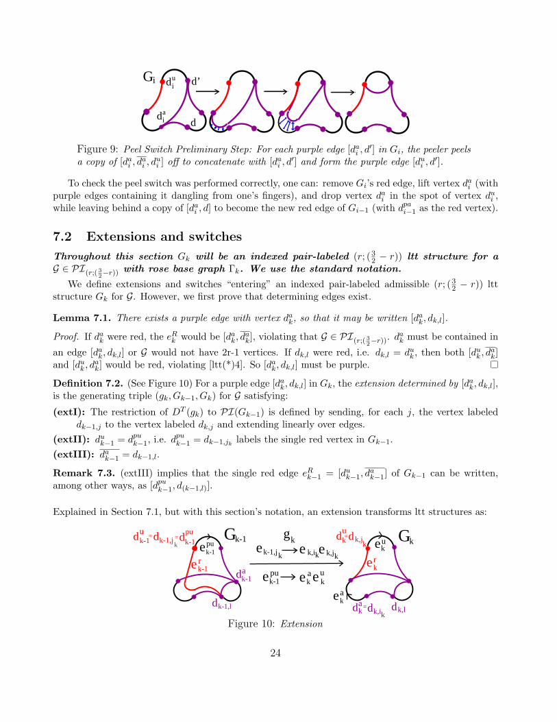
d

d’Gi

dai

diu

Figure 9: Peel Switch Preliminary Step: For each purple edge [dai , d′] in Gi, the peeler peels

a copy of [dai , dai , d

ui ] off to concatenate with [dai , d

′] and form the purple edge [dui , d′].

To check the peel switch was performed correctly, one can: remove Gi’s red edge, lift vertex dai (withpurple edges containing it dangling from one’s fingers), and drop vertex dai in the spot of vertex dui ,while leaving behind a copy of [dai , d] to become the new red edge of Gi−1 (with dpai−1 as the red vertex).

7.2 Extensions and switches

Throughout this section Gk will be an indexed pair-labeled (r; (32 − r)) ltt structure for aG ∈ PI(r;( 3

2−r)) with rose base graph Γk. We use the standard notation.

We define extensions and switches “entering” an indexed pair-labeled admissible (r; (32 − r)) lttstructure Gk for G. However, we first prove that determining edges exist.

Lemma 7.1. There exists a purple edge with vertex dak, so that it may be written [dak, dk,l].

Proof. If dak were red, the eRk would be [dak, dak], violating that G ∈ PI(r;( 3

2−r)). d

ak must be contained in

an edge [dak, dk,l] or G would not have 2r-1 vertices. If dk,l were red, i.e. dk,l = duk , then both [duk , dak]

and [duk , dak] would be red, violating [ltt(*)4]. So [dak, dk,l] must be purple.

Definition 7.2. (See Figure 10) For a purple edge [dak, dk,l] in Gk, the extension determined by [dak, dk,l],is the generating triple (gk, Gk−1, Gk) for G satisfying:

(extI): The restriction of DT (gk) to PI(Gk−1) is defined by sending, for each j, the vertex labeleddk−1,j to the vertex labeled dk,j and extending linearly over edges.

(extII): duk−1 = dpuk−1, i.e. dpuk−1 = dk−1,jk labels the single red vertex in Gk−1.

(extIII): dak−1 = dk−1,l.

Remark 7.3. (extIII) implies that the single red edge eRk−1 = [duk−1, dak−1] of Gk−1 can be written,

among other ways, as [dpuk−1, d(k−1,l)].

Explained in Section 7.1, but with this section’s notation, an extension transforms ltt structures as:

duk=d

kk,j

dk=d

k

ak,i dk,l

dk-1,lka

ekr

Gk

k-1

e

e r

dak-1

dk-1pu

=dk-1u

= dk-1,jk

Gk-1 gke e ek-1,jk k,jkk,ik

e e epuk-1

ak

uk

epuk-1

euk

Figure 10: Extension

24

Lemma 7.4. Given an edge [dak, dk,l] in PI(Gk), the extension (gk, Gk−1, Gk) determined by [dak, dk,l]is unique.I. Gk−1 can be obtained from Gk by the following steps:

1. removing the interior of the red edge from Gk;2. replacing each vertex label dk,i with dk−1,i and each vertex label dk,i with dk−1,i; and3. adding a red edge eRk−1 connecting the red vertex to dk−1,l.

II. The fold is such that the corresponding homotopy equivalence maps the oriented ek−1,jk ∈ Ek−1 overthe path ek,ikek,jk in Γk and then each oriented ek−1,t ∈ Ek−1 with ek−1,t = e±1

k−1,jkover ek,t.

Proof. The proof is an unraveling of definitions. A full presentation can be found in [Pfa12].

Definition 7.5. (See Figure 11) The switch determined by a purple edge [dak, d(k,l)] in Gk is thegenerating triple (gk, Gk−1, Gk) for G satisfying:

(swI): DT (gk) restricts to an isomorphism from PI(Gk−1) to PI(Gk) defined by

PI(Gk−1)dpuk−1 7→dak=dk,ik−−−−−−−−−−→ PI(Gk)

(dk−1,t 7→ dk,t for dk−1,t = dpuk−1) and extended linearly over edges.

(swII): dpak−1 = duk−1.

(swIII): dak−1 = dk−1,l.

Remark 7.6. (swII) implies that the red edge eRk−1 = [duk−1, dak−1] of Gk−1 can be written [dpak−1, d

ak−1],

among other ways. (swIII) implies that eRk−1 can be written [d(k−1,ik), d(k−1,l)].

Explained in Section 7.1, but with this section’s notation, a switch transforms ltt structures as follows:

duk

=dk

k,j

dk= d

k

ak,i dk,l

ka

Gk

e

dak-1

dk-1pu

dk-1u

= dk-1,jkGk-1

= dk-1,ik=dk-1

pa dk-1,l

gke e ek-1,jk k,jkk,ik

e e epuk-1

ak

uk

epuk-1 e a

k-1

e uk

Figure 11: Switch

Lemma 7.7. Given an edge [dak, dk,l] in PI(Gk), the switch (gk, Gk−1, Gk) determined by [dak, dk,l] isunique.

I. Gk−1 can be obtained from Gk by the following steps:

1. Start with PI(Gk).2. Replace each vertex label dk,i with dk−1,i.3. Switch the attaching (purple) vertex of the red edge to be dk−1,l.4. Switch the labels d(k−1,jk) and d(k−1,ik), so that the red vertex of Gk−1 will be dk−1,ik and the

red edge of Gk−1 will be [d(k−1,ik), d(k−1,l)].

25

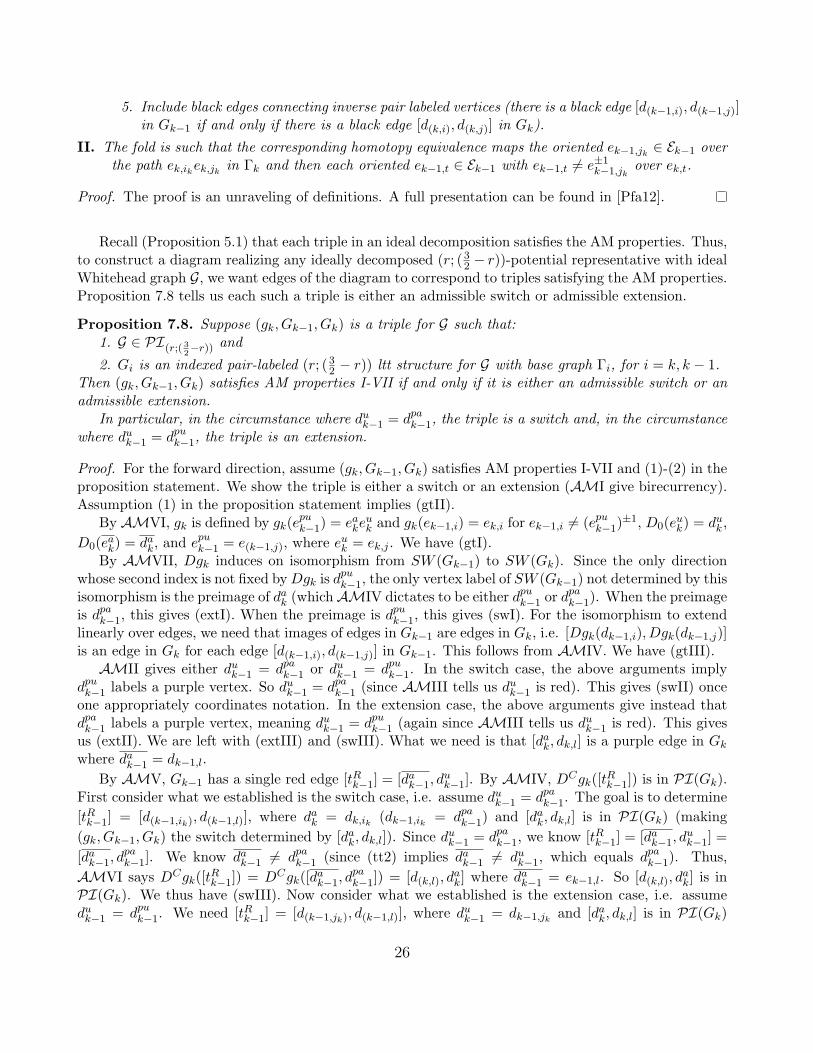
5. Include black edges connecting inverse pair labeled vertices (there is a black edge [d(k−1,i), d(k−1,j)]in Gk−1 if and only if there is a black edge [d(k,i), d(k,j)] in Gk).

II. The fold is such that the corresponding homotopy equivalence maps the oriented ek−1,jk ∈ Ek−1 overthe path ek,ikek,jk in Γk and then each oriented ek−1,t ∈ Ek−1 with ek−1,t = e±1

k−1,jkover ek,t.

Proof. The proof is an unraveling of definitions. A full presentation can be found in [Pfa12].

Recall (Proposition 5.1) that each triple in an ideal decomposition satisfies the AM properties. Thus,to construct a diagram realizing any ideally decomposed (r; (32 − r))-potential representative with idealWhitehead graph G, we want edges of the diagram to correspond to triples satisfying the AM properties.Proposition 7.8 tells us each such a triple is either an admissible switch or admissible extension.

Proposition 7.8. Suppose (gk, Gk−1, Gk) is a triple for G such that:1. G ∈ PI(r;( 3

2−r)) and

2. Gi is an indexed pair-labeled (r; (32 − r)) ltt structure for G with base graph Γi, for i = k, k − 1.Then (gk, Gk−1, Gk) satisfies AM properties I-VII if and only if it is either an admissible switch or anadmissible extension.

In particular, in the circumstance where duk−1 = dpak−1, the triple is a switch and, in the circumstancewhere duk−1 = dpuk−1, the triple is an extension.

Proof. For the forward direction, assume (gk, Gk−1, Gk) satisfies AM properties I-VII and (1)-(2) in theproposition statement. We show the triple is either a switch or an extension (AMI give birecurrency).Assumption (1) in the proposition statement implies (gtII).

By AMVI, gk is defined by gk(epuk−1) = eake

uk and gk(ek−1,i) = ek,i for ek−1,i = (epuk−1)

±1, D0(euk) = duk ,

D0(eak) = dak, and epuk−1 = e(k−1,j), where e

uk = ek,j . We have (gtI).

By AMVII, Dgk induces on isomorphism from SW (Gk−1) to SW (Gk). Since the only directionwhose second index is not fixed byDgk is d

puk−1, the only vertex label of SW (Gk−1) not determined by this

isomorphism is the preimage of dak (whichAMIV dictates to be either dpuk−1 or dpak−1). When the preimage

is dpak−1, this gives (extI). When the preimage is dpuk−1, this gives (swI). For the isomorphism to extendlinearly over edges, we need that images of edges in Gk−1 are edges in Gk, i.e. [Dgk(dk−1,i), Dgk(dk−1,j)]is an edge in Gk for each edge [d(k−1,i), d(k−1,j)] in Gk−1. This follows from AMIV. We have (gtIII).

AMII gives either duk−1 = dpak−1 or duk−1 = dpuk−1. In the switch case, the above arguments implydpuk−1 labels a purple vertex. So duk−1 = dpak−1 (since AMIII tells us duk−1 is red). This gives (swII) onceone appropriately coordinates notation. In the extension case, the above arguments give instead thatdpak−1 labels a purple vertex, meaning duk−1 = dpuk−1 (again since AMIII tells us duk−1 is red). This givesus (extII). We are left with (extIII) and (swIII). What we need is that [dak, dk,l] is a purple edge in Gk

where dak−1 = dk−1,l.

By AMV, Gk−1 has a single red edge [tRk−1] = [dak−1, duk−1]. By AMIV, DCgk([t

Rk−1]) is in PI(Gk).

First consider what we established is the switch case, i.e. assume duk−1 = dpak−1. The goal is to determine

[tRk−1] = [d(k−1,ik), d(k−1,l)], where dak = dk,ik (dk−1,ik = dpak−1) and [dak, dk,l] is in PI(Gk) (making

(gk, Gk−1, Gk) the switch determined by [dak, dk,l]). Since duk−1 = dpak−1, we know [tRk−1] = [dak−1, d

uk−1] =

[dak−1, dpak−1]. We know dak−1 = dpak−1 (since (tt2) implies dak−1 = duk−1, which equals dpak−1). Thus,

AMVI says DCgk([tRk−1]) = DCgk([d

ak−1, d

pak−1]) = [d(k,l), d

ak] where d

ak−1 = ek−1,l. So [d(k,l), d

ak] is in

PI(Gk). We thus have (swIII). Now consider what we established is the extension case, i.e. assumeduk−1 = dpuk−1. We need [tRk−1] = [d(k−1,jk), d(k−1,l)], where d

uk−1 = dk−1,jk and [dak, dk,l] is in PI(Gk)

26

(making (gk, Gk−1, Gk) the extension determined by [dak, dk,l]). Since duk−1 = dpuk−1, we know [tRk−1] =

[dak−1, duk−1] = [dak−1, d

puk−1]. We know dak−1 = dpuk−1 (since (tt2) implies dak−1 = duk−1, which equals

dpuk−1). Thus, by AMVI, DCgk([tRk−1]) = DCgk([d

ak−1, d

puk−1]) = [d(k,l), d

ak], where d

ak−1 = ek−1,l. We have

(extIII) and the forward direction.For the converse, assume (gk, Gk−1, Gk) is either an admissible switch or extension. Since we required

extensions and switches be admissible, Gk−1 and Gk are birecurrent. We have AMI.The first and second parts of AMII are equivalent and the second part holds by (extII) for an

extension and (swII) for a switch. For AMIII note that there is only a single red vertex (labeledduk) in Gk and is only a single red vertex (labeled duk−1) in Gk−1 because of the requirement in (gtII)

that Gk and Gk−1 are (r; (32 − r)) ltt structures (see the standard notation for why this is notationallyconsistent with the AM properties). What is left of AMIII is that the edge [tRk ] = [duk , d

ak] in Gk and

the edge [tRk−1] = [duk−1, dak−1] in Gk−1 are both red. This follows from (gtI) combined with (extII) for

an extension and (swII) for a switch.(gtIII) implies AMIV. For AMV, note: AMIII implies eRk is a red edge containing the red vertex

duk . (ltt(*)4) implies the uniqueness of both the red edge and direction.Since AMVI follows from (gtI), combined with (extII) for an extension and (swII) for a switch, and

AMVII follows from (gtIII), we have proved the converse.

Definition 7.9. In light of Proposition 7.8, an admissible map will mean a triple for a G ∈ PI(r;( 32−r))

that is an admissible switch or admissible extension or (equivalently) satisfies AM properties I-VII.

8 Ideal decomposition (ID) diagrams

Throughout this section G ∈ PI(r;( 32−r)). We define the “ideal decomposition (ID) diagram” for G,

as well as prove that representatives with (r; (32 − r)) potential are realized as loops in these diagrams.We use ID diagrams to prove Theorem 9.1B and to construct examples in [Pfa13b].

Definition 8.1. A preliminary ideal decomposition diagram for G is the directed graph where

1. the nodes correspond to equivalence classes of admissible indexed pair-labeled (r; (32−r)) ltt struc-tures for G and

2. for each equivalence class of an admissible generator triple (gi, Gi−1, Gi) for G, there exists adirected edge E(gi, Gi−1, Gi) from the node [Gi−1] to the node [Gi].

The disjoint union of the maximal strongly connected subgraphs of the preliminary ideal decompositiondiagram for G will be called the ideal decomposition (ID) diagram for G (or ID(G)).

Remark 8.2. [Pfa12] gives a procedure for constructing ID diagrams (there called “AM Diagrams”).

We say an ideal decomposition Γ0g1−→ Γ1

g2−→ · · · gk−1−−−→ Γk−1gk−→ Γk of a tt g with indexed (r; (32 − r))

ltt structures G0 → G1 → · · · → Gk−1 → Gk for G is realized by E(g1, G0, G1) ∗ · · · ∗E(gk, Gk−1, Gk) inID(G) if the oriented path E(g1, G0, G1) ∗ · · · ∗E(gk, Gk−1, Gk) in ID(G) from [G0] to [Gk], traversingthe E(gi, Gi−1, Gi) in order of increasing i (from E(g1, G0, G1) to E(gk, Gk−1, Gk)), exists.

Proposition 8.3. If g = gk ◦ · · · ◦ g1, with ltt structures G0 → G1 → · · · → Gk−1 → Gk, is an ideallydecomposed representative of ϕ ∈ Out(Fr), with (r; (32 − r)) potential, such that IW(ϕ) = G, thenE(g1, G0, G1) ∗ · · · ∗ E(gk, Gk−1, Gk) exists in ID(G) and forms an oriented loop.

27

Proof. This follows from Proposition 7.8 and Proposition 5.1.

Corollary 8.4. (of Proposition 8.3) If no loop in ID(G) gives a potentially-(r; (32−r)) representativeof a ϕ ∈ Out(Fr) with IW(ϕ) = G, such a ϕ does not exist. In particular, any of the following ID(G)properties would prove such a representative does not exist:

1. For at least one edge pair {di, di}, where ei ∈ E(Γ), no red vertex in ID(G) is labeled by d±1i .

2. The representative corresponding to each loop in ID(G) has a pNp.

As a result of Corollary 8.4(1) we define:

Definition 8.5. Irreducibility Potential Test: Check whether, in each connected component ofID(G), for each edge vertex pair {di, di}, there is a node N in the component such that either di or dilabels the red vertex in the structure N . If it holds for no component, G is unachieved.

Remark 8.6. Let {x1, x1, . . . , x2r, x2r} be a rank-r edge pair labeling set. We call a permutation ofthe indices 1 ≤ i ≤ 2r combined with a permutation of the elements of each pair {xi, xi} an Edge Pair(EP) Permutation. Edge-indexed graphs will be considered Edge Pair Permutation (EPP) isomorphicif there is an EP permutation making the labelings identical (this still holds even if only a subset of{x1, x1, . . . , x2r, x2r} is used to label the vertices, as with a graph in PI(r;( 3

2−r))).

When checking for irreducibility, it is only necessary to look at one EPP isomorphism class of eachcomponent (where two components are in the same class if one can be obtained from the other byapplying the same EPP isomorphism to each triple in the component).

9 Several unachieved ideal Whitehead graphs

Theorem 9.1. For each r ≥ 3, let Gr be the graph consisting of 2r−2 edges adjoined at a single vertex.

A. For no fully irreducible ϕ ∈ Out(Fr) is IW(ϕ) ∼= Gr.

B. The following connected graphs are not the ideal Whitehead graph IW(ϕ) for any fully irreducibleϕ ∈ Out(F3):

Proof. We first prove (A). By Proposition 4.4, it suffices to show that no admissible (r; (32 − r)) lttstructure for G is birecurrent. Up to EPP-isomorphism, there are two such ltt structures to consider,neither birecurrent):

andv1

v1

v1

v1

These are the only structures worth considering as follows: Call the valence-(2r − 2) vertex v1. Either(1) some valence-1 vertex is labeled by v1 or (2) the set of valence-1 vertices {x1, x1, . . . , xr−1, xr−1}consists of r − 1 edge-pairs. Suppose (2) holds. The red edge cannot be attached in such a way that itis labeled with an edge-pair or is a loop and attaching it to any other vertex yields an EPP-isomorphicltt structure to that on the left. Suppose (1) holds. Let xi label the red vertex. The valence-1 vertex

28

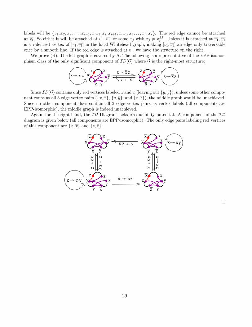
labels will be {v1, x2, x2, . . . , xi−1, xi−1, xi, xi+1, xi+1, xi . . . , xr, xr}. The red edge cannot be attachedat xi. So either it will be attached at v1, v1, or some xj with xj = x±1

i . Unless it is attached at v1, v1is a valence-1 vertex of [v1, v1] in the local Whitehead graph, making [v1, v1] an edge only traversableonce by a smooth line. If the red edge is attached at v1, we have the structure on the right.

We prove (B). The left graph is covered by A. The following is a representative of the EPP isomor-phism class of the only significant component of ID(G) where G is the right-most structure:

x

z y y

zxz z

xx zzx x z zx

y z

x zy

x

x

Since ID(G) contains only red vertices labeled z and x (leaving out {y, y}), unless some other compo-nent contains all 3 edge vertex pairs ({x, x}, {y, y}, and {z, z}), the middle graph would be unachieved.Since no other component does contain all 3 edge vertex pairs as vertex labels (all components areEPP-isomorphic), the middle graph is indeed unachieved.

Again, for the right-hand, the ID Diagram lacks irreducibility potential. A component of the IDdiagram is given below (all components are EPP-isomorphic). The only edge pairs labeling red verticesof this component are {x, x} and {z, z}:

z

y

y zx

zz

xz

y y

zx

zz

x

x

xz z

x

xx

zxx y

zzx

y

z

x

y

z

y

x

zx

y

z

yx

y

xy

xz

29

References

[BF94] M. Bestvina and M. Feighn, Outer limits, preprint (1994), 1–19.

[BFH97] M. Bestvina, M. Feighn, and M. Handel, Laminations, trees, and irreducible automorphismsof free groups, Geometric and Functional Analysis 7 (1997), no. 2, 215–244.

[BFH00] , The Tits alternative for Out(Fn) I: Dynamics of exponentially-growing automor-phisms, Annals of Mathematics-Second Series 151 (2000), no. 2, 517–624.

[BH92] M. Bestvina and M. Handel, Train tracks and automorphisms of free groups, The Annals ofMathematics 135 (1992), no. 1, 1–51.

[CV86] M. Culler and K. Vogtmann, Moduli of graphs and automorphisms of free groups, Inventionesmathematicae 84 (1986), no. 1, 91–119.

[GJLL98] D. Gaboriau, A. Jaeger, G. Levitt, and M. Lustig, An index for counting fixed points ofautomorphisms of free groups, Duke mathematical journal 93 (1998), no. 3, 425–452.

[HM07] M. Handel and L. Mosher, Parageometric outer automorphisms of free groups, Transactionsof the American Mathematical Society 359 (2007), no. 7, 3153–3184.

[HM11] , Axes in Outer Space, no. 1004, Amer Mathematical Society, 2011.

[JL09] A. Jager and M. Lustig, Free group automorphisms with many fixed points at infinity, arXivpreprint arXiv:0904.1533 (2009).

[Mah11] J. Maher, Random walks on the mapping class group, Duke Mathematical Journal 156 (2011),no. 3, 429–468.

[MS93] H. Masur and J. Smillie, Quadratic differentials with prescribed singularities and pseudo-Anosov diffeomorphisms, Commentarii Mathematici Helvetici 68 (1993), no. 1, 289–307.

[NH86] J. Nielsen and V.L. Hansen, Jakob Nielsen, Collected Mathematical Papers: 1913-1932, vol. 1,Birkhauser, 1986.

[Pfa12] C. Pfaff, Constructing and Classifying Fully Irreducible Outer Automor-phisms of Free Groups, Ph.D. thesis, Rutgers University, 2012, PhD Thesis,http://www.math.rutgers.edu/~cpfaff/Thesis.pdf.

[Pfa13a] Catherine Pfaff, Ideal Whitehead Graphs in Out(Fr) II: The Complete Graph in Each Rank,arXiv preprint arXiv:1301.6645 (2013).

[Pfa13b] , Ideal Whitehead Graphs in Out(Fr) III: Achieved Graphs in Rank 3, arXiv preprintarXiv:1301.7080 (2013).

[Sko89] R. Skora, Deformations of length functions in groups, preprint, Columbia University (1989).

[Sta83] J.R. Stallings, Topology of finite graphs, Inventiones Mathematicae 71 (1983), no. 3, 551–565.

30