GRIPS Discussion Paper 15-20

ICT for Financial Inclusion: Mobile Money and the Financial Behavior

of Rural Households in Uganda

Ggombe Kasim Munyegera Tomoya Matsumoto

【Emerging State Project】

December 2015

National Graduate Institute for Policy Studies

7-22-1 Roppongi, Minato-ku,

Tokyo, Japan 106-8677

1

ICT for Financial Inclusion: Mobile Money and the Financial Behavior of Rural Households in Uganda∗

Ggombe Kasim Munyegera† and Tomoya Matsumoto‡

December, 2015

Abstract

Over 35 percent of the adult use mobile money services in 2014, just five years since its

inception in Uganda. Using household survey data covering 820 rural households, we

examine the effect of this financial innovation on their financial behavior. We find that

adopting mobile money services significantly increases the likelihood of saving, borrowing

and receiving remittances due to reduction in transaction cost. The amount of savings, credit

and remittances is also significantly higher among user households than non-users. To

illustrate the importance of service proximity, we show that reducing the distance to the

nearest mobile money agent boosts the frequency of using mobile money services. Our

results are robust to specification changes and alternative explanations.

Key words: mobile money, financial inclusion, rural households, financial services, Uganda.

JEL (O16, O17, O33, I131)

*This work was supported by MEXT (Ministry of Education, Culture, Sports, Science and Technology), Global Center of Excellency and JSPS KANENHI Grant Number 25101002. All errors remain ours. †Munyegera: Corresponding author/presenter; National Graduate Institute for Policy Studies, 7-22-1 Roppongi, Minato-ku, Tokyo106-8677, Japan (email: kasimgm@gmail.com) ‡Matsumoto: Co-author; National Graduate Institute for Policy Studies, 7-22-1 Roppongi, Minato-ku, Tokyo106-8677, Japan (email: tmatsumo@grips.ac.jp)

2

1. Introduction

Financial sector development is a crucial element of the development process as it improves

the mobilization of savings, allocation of capital funds, monitoring of the use of funds and

aiding in risk management (Levine, 1997). Access to financial services like saving, money

transfer, insurance and credit has enormous potential to shape people’s livelihoods through

poverty and vulnerability reduction (Jalilian and Kirkpatrick, 2005; Beck et al., 2004;

Demirguc-Kunt et al., 2008; Odhiambo, 2009). However, majority of the world’s poor have

no access to these basic financial services (Demirgüç-Kunt and Klapper, 2012). The lack of

access to affordable financial services limits their ability to smooth consumption and

undertake productive investments. The rural poor in developing countries have the least

access to such services and ultimately, their capacity to escape chronical poverty is greatly

curtailed (Dupas and Robinson, 2008).

Mobile money has been dramatically changing the situation since its recent inception

in some developing countries. Mobile money is a financial product that allows users to make

basic financial transactions via a mobile phone. This financial innovation has come to the

limelight in the financial access literature over the recent years because of its potential to

foster financial access especially among the financially excluded rural poor in developing

countries (Jack and Suri, 2011; Hughes and Lonie, 2007). Indeed, mobile money has

expanded rapidly over the past decade especially in the developing world where the

penetration rate of formal financial services is very low. The dramatic expansion of mobile

phone network coverage, combined with the rapid adoption of mobile phone devices in the

3

past decade explains much of the success registered by Mobile Money in low-income

countries (USAID, 2010). The period between 2000 and 2011 has been dubbed the mobile

revolution decade, with mobile phone subscriptions increasing from 10 percent to 80 percent

(IC4D, 2012).1 Approximately 79 percent of the population in developing countries had

access to a mobile phone by the end of 2011 while over 50 percent of Africans owned a

mobile phone in 2009, compared to 20 percent with a formal bank account (McKinsey, 2009).

There has been a growing body of literature that identifies the factors behind the high

incidence of financial exclusion, including socio-cultural factors (Sarma and Pais, 2011;

Johnson and Nino-Zarazua, 2011), long distance to the financial institution (Pedrosa and Do,

2011) and high cost of account maintenance (Dupas and Robinson, 2013).2 In low-income

countries, formal financial institutions like commercial banks and deposit-taking micro-

finance institutions are concentrated in urban centers. This implies that access to formal

financial services by the rural populace is complicated by the long and costly treks made to

access service points in urban locations. Besides, the high cost of operating a bank account

imposes a challenge to the adoption of formal financial services especially among the low-

income people. An experimental study by Dupas and Robinson (2013) reveals that access to

non-interest-bearing savings accounts increased savings and investments among market

vendors in Kenya. The study emphasizes the importance of service cost as a critical factor in

the uptake of financial services among low-income communities.

1 Information and Communication for Development 2 Financially excluded constitutes individuals who cannot either access or afford to use the services offered

4

The lack of access to a formal financial institution in rural communities imposes a

high cost of transferring money especially over long distances and this is often exacerbated

by poor road conditions. Physical transfer of money is a common channel of remittances

among the financially excluded rural communities despite the relatively high risk of theft and

the high transport and time cost involved in this exchange mechanism. The low cost of mobile

banking relative to conventional banking implies an increase in the flow of remittances

among family members and friends (Mbiti and Weil, 2011) which greatly improves the

welfare of recipient households (Munyegera and Matsumoto, forthcoming). The general lack

of access to formal financial institutions partly accounts for the rapid adoption of mobile

money services as an invaluable alternative for the financially excluded rural poor (World

Economic Forum report, 2011).

Empirical research on informal insurance and risk sharing indicate that the

availability of a cheap remittance channel increases the incidence of risk sharing and reduces

vulnerability to income and consumption shocks. Using panel data from Kenya, Jack and

Suri (2014) illustrated that households that used M-PESA - Kenya’s most famous mobile

money platform – were able to receive remittances to offset the effect of illness and weather

shocks which caused a notable reduction in consumption expenditure among non-user

households. Although most studies on mobile banking concentrate on peer-to-peer transfer

services, which is the most common service offered across the mobile money platform given

its infancy, the product supports business to person, business-to-business and government-

to-person services at a relatively lower cost than conventional transfer platforms like

commercial banks. A study by Aker et al. (2011) in Niger demonstrated that the use of mobile

5

banking reduced the cost to the government and recipients of a welfare program that

distributed financial assistance to the people affected by the critical drought of 2008.

Despite the increasing importance of mobile banking, there is little empirical

evidence on the potential of this financial innovation with regards to services beyond money

transfer. Mobile money now offers a broader range of services including an integrated access

to formal bank services through partnerships between Mobile Network Operators (MNOs)

and registered commercial banks and deposit-taking microfinance institutions (MFIs). Other

services like the electronic payment of school fees, salaries and utility bills (in principle,

water and electricity) are expected to reduce the frequencies of cash transactions and increase

financial efficiency (USAID, 2012). Safaricom’s M-PESA in Kenya now offers an integrated

financial package with extended services like microsavings, credit and agricultural insurance

through customized platforms called M-KESHO and Kilimo Safi. It is documented that access

to an affordable savings platform can change financial behaviors of households by reducing

wasteful expenditure and saving with informal platforms (Morawczynski and Pickens 2009).

Although considerable effort has been devoted to studying the developmental impact

of mobile money in the areas of remittances, risk sharing and consumption smoothing,

empirical evidence on its potential to boost savings, credit, insurance and mobile payments

remains largely missing. In the context of Uganda, mobile money studies focus on the

determinants of adoption (Johnson and Nino-Zarazua, 2011) while others rely on small and

less-representative samples (Ndiwalana, 2010). The objective of this study is to fill literature

gap by analyzing the effect of mobile money on the saving, credit and remittance behaviors

6

of rural households in Uganda. The study is expected to contribute to the existing literature

by assessing the potential of mobile money to enhance financial inclusion, extending the

analysis beyond peer-to-peer remittances to savings and credit.

The rest of the paper is organized as follows; Section 2 provides background

information on mobile money in Uganda and Section 3 describes the survey data and their

summary statistics. We describe the empirical strategy in Section 4 and provide our results

in Section 5 while Section 6 concludes the analysis.

2. Development of mobile money service in Uganda.

In March 2009, Mobile Telephone Network (MTN) – the leading Mobile Network Operator

in the country – established MTN Mobile Money, the first mobile money platform in the

country, inspired by the massive success of Safaricom’s M-PESA in Kenya. Airtel Uganda,

formerly known as Zain, joined the service when it rolled out its Airtel Money in June the

same year. This new financial innovation proved to be an efficient way for telecom

companies to increase their market shares by widening the range of services available to their

clients. This attracted Uganda Telecom to introduce M-Sente in March 2010, followed by

Warid Pesa from Warid Telecom in December 2011 and Orange Money from Orange

Telecom in the first half of 2012 (Uganda Communications Commission-UCC 2012).

Since mobile money was established in Uganda, the number of subscribers has been

steadily increasing. By mid-2014, over 17.6 million Ugandans had adopted mobile money

services, representing over a five-fold expansion from 3 million users in 2011. In the same

period, the number of mobile money transactions increased from 180 million to 242 million

7

and the corresponding total value exchanged through the platform increased from $1.5 billion

to $4.5 billion in the same period (BoU, 2012). The MTN Mobile Money alone has over

15,000 agents as compared with 455 commercial bank branches with 660 Automated Teller

Machines (ATMs).3 This rapid expansion partly owes to the high rates of both the roll-out of

mobile phone networks and adoption of mobile phones. In our survey sample households,

the proportion of households owning a mobile phone increased from 73 percent to 90 percent

between 2012 and 2014 while all of the Local Council 1s (hereafter called LC1s) were

covered by mobile phone network in both rounds. 4 One in four households reported

possessing more than one mobile phone in the Mobile Money survey of 2014 (hereafter

referred to as MM2014).

Mobile money allows users to deposit money as e-float on a SIM card-based account,

called an m-wallet, which can be converted into cash at any mobile money agent located all

over the country. In the initial stage of its establishment, the range of services offered was

largely limited to person-to-person money transfer. However, with the growing interest from

stake-holders, coupled with competition among the mobile network operators (MNOs),

service providers have gradually innovated to widen the range of services. Currently, most

MNOs offer more complex functions like payment of utility bills, school fees, airtime

purchase, direct purchase of goods and services and, to some extent, payment of government

taxes. Recent developments in the mobile banking arena have made it possible for users to

access their bank accounts using their mobile phones without having to physically visit their

3 Mobile money agents serve as outlet centers or cash points where users can exchange their e-float for cash and vice versa. 4 LC1 is the smallest administrative unit in Uganda.

8

bank branches, thanks to the partnership between MNOs and commercial banks.5 This is

expected to raise financial inclusion especially at the lower end of the socio-economic

spectrum while reducing the cost of access to and use of basic financial services.

With the rapid urbanization in Uganda over the past years, the number of people

migrating to urban centers has been steadily increasing, most often in pursuit of jobs. Those

who migrate to cities often extend financial support to their family members and friends in

villages in the form of remittances and informal loans. The efficiency of this remittance

system used to heavily rely on the quality of transport infrastructure as most of these

transactions were traditionally made through informal channels like physical movement of

cash by the receiver, sender, and agents like bus and taxi drivers. Besides, the massive

geographical dispersion between senders and receivers implies high transaction costs in

terms of transport fares and travel time involved in sending and receiving money among

family members and friends especially across geographically distant and remote locations.

This background motivates our postulation that mobile money lowers the time, transport and

other transaction costs associated with the usage of financial services, catalyzing their

adoption even by rural households. Similarly, the financial product has made it easier for

friends and relatives to exchange informal credit while others find it convenient and cost-

effective to save money over the m-wallet in instances where commercial banks are

inaccessible.

5Major partnerships exist between MTN Mobile Money and Stanbic Bank, M-Sente and Standard Chartered Bank and WaridPesa and DFCU Bank.

9

3. Data and Summary Statistics

This paper uses a combination of two data sources - the Research on Poverty, Environment

and Agricultural Technology (RePEAT) and MM2014. The RePEAT is a panel household

survey conducted jointly by the National Graduate Institute for Policy Studies (GRIPS), the

Foundation for Advanced Studies on International Development (FASID) and Makerere

University in four rounds between 2003 and 2012.

The survey collected detailed information on household consumption, incomes,

agricultural production from 940 rural households in 94 LC1s. We followed up 916

households that were interviewed in the last round of the RePEAT in 2012 and conducted a

MM2014 among these households between June and July 2014 particularly in order to collect

the detail information on the use of financial services. We successfully interviewed 820 out

of the 916 households and asked questions about the usage of mobile money, banks, Savings

and Credit Associations (SACCOs) and Micro-finance Institutions (MFIs) as well as

financial services including savings, remittances and credit (both formal and informal).

Analysis is based on 820 households that were interviewed in 2014, constructing financial

access and usage variables from the MM2014 while information on household characteristics

is obtained from RePEAT4.6 The choice of rural households as our analysis sample is

intended to portray the contribution of mobile money among the rural poor who are often

excluded from the formal financial system.

6 We were unable to construct a panel because financial access and usage variables are not available in RePEAT surveys except mobile money adoption and remittances transactions.

10

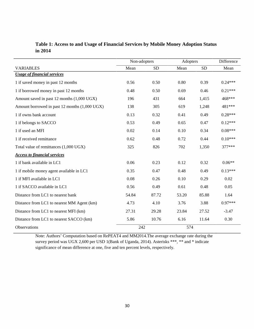
We provide summary statistics for financial access and usage by mobile money

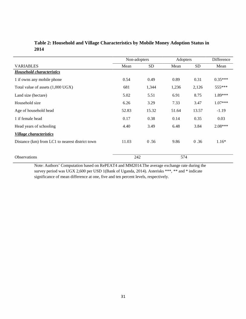
adoption status in Table 1 and household and village characteristics in Table 2. During just

two years between the RePEAT4 and the MM2014, the proportion of households with at

least one mobile money user increased almost two-fold from 38 percent to 70 percent and

barely one percent of the sample households had a mobile money user in the third round of

the RePEAT in 2009. This reflects a rapid penetration within just five years since mobile

money was introduced in Uganda in 2009. The rapid adoption of mobile money services is

partly attributed to the high adoption rate of mobile phones and the lack of rural coverage by

formal financial institutions.7 Over 80 percent of the households in the MM2014 had at least

one mobile phone with one in four households possessing more than one handset. The

significantly higher rate of mobile phone possession among mobile money users is not

surprising given the nature of the mobile money platform which uses the mobile phone as

infrastructure for the services offered. In contrast, only 41 and 13 percent of mobile money

adaptors and non-adaptors have at least one bank account, respectively. Table 2 further

shows that households that adopt mobile money services have more educated heads with an

average difference of two years of schooling.

Peer-to-peer remittance is the most commonly adopted function of the mobile money

platform. The proportion of mobile money users who report having received remittances at

least once in the 12 months before the MM2014 interview date is thus ten percent higher

compared to non-users. Similarly, the amount of remittances received is twice as high at

7 These include commercial banks and deposit-taking MFIs.

11

UGX 702,000 (USD 270) and UGX 325,000 (USD 125) for users and non-users, respectively.

The user households are also more likely to save and borrow money and the amount saved

and borrowed is significantly higher. We postulate that mobile money provides a convenient

channel not only for remittances but also for short-term savings mainly for school fees to be

drawn at the onset of a new school term or for purchasing agricultural inputs when the

planting season starts.8 Mobile money users are generally wealthier than non-users in terms

of both asset and land endowments.

The user households tend to be less female-headed and have younger heads than the

non-users. Regarding physical access to financial service providers, the user households are

located one kilometer closer to the mobile money agent than the non-user households while

there are no significant differences in distance to banks because our sample is predominantly

rural and majority of banks are located in the district town which is, on average, tens of

kilometers away from the village center. Although there are systematic differences in the

individual and LC1 level characteristics between the mobile money users and non-users, the

simple comparison of their outcome variables on savings, credit use, and remittance receipt

would not identify the causal effect of adoption of the mobile money. Thus, we discuss about

our identification strategy in the following section.

[ Insert Table 1 here ]

8 According to the survey data and also the observation through focus group discussions, the two main purposes of receiving remittances, saving and borrowing money in the sample are to raise school fees and make farm investments which include hiring labor and buying inputs.

12

4. Empirical Strategy

4.1. Adoption of Financial Services

A household’s decision to use a particular financial service depends on household and

community characteristics in the form:

𝑆𝑆𝑆𝑆𝑆𝑆𝑆𝑆𝑆𝑆𝑆𝑆𝑆𝑆𝑖𝑖𝑖𝑖𝑖𝑖ℎ = 1{𝛽𝛽𝑀𝑀ℎ𝑀𝑀𝑀𝑀𝑀𝑀𝑀𝑀𝑆𝑆𝑀𝑀𝑖𝑖𝑖𝑖𝑖𝑖 + 𝛽𝛽1ℎ𝑋𝑋𝑖𝑖𝑖𝑖𝑖𝑖 + 𝛽𝛽2ℎ𝑉𝑉𝑖𝑖𝑖𝑖 + 𝜂𝜂𝑖𝑖ℎ + 𝜀𝜀𝑖𝑖𝑖𝑖𝑖𝑖ℎ > 0}, (1)

where 𝑆𝑆𝑆𝑆𝑆𝑆𝑆𝑆𝑆𝑆𝑆𝑆𝑆𝑆𝑖𝑖𝑖𝑖𝑖𝑖ℎ is a dummy variable taking one if the household i living in the village j of

the district d has at least one member who uses z financial service h, and h comprises of

savings, credit and remittances. 𝑀𝑀𝑀𝑀𝑀𝑀𝑀𝑀𝑆𝑆𝑀𝑀𝑖𝑖𝑖𝑖𝑖𝑖 is a dummy variable taking one if the household

has at least one member who uses mobile money services. The parameter ɳd captures district

fixed effects. Xijd is a vector of household characteristics which include household size, log

of asset value and land endowments, age, gender and education level of the household head.

Vjd is a vector of observed village characteristics that could potentially influence the

household’s decision on the use of those financial services. These include a distance measure

in kilometers from the village center to the nearest district town and also distance measures

to the nearest respective service providers. 𝜀𝜀𝑖𝑖𝑖𝑖𝑖𝑖ℎ is a disturbance term. Under the

independence assumption of the disturbance term from the mobile money dummy,

𝑀𝑀𝑀𝑀𝑀𝑀𝑀𝑀𝑆𝑆𝑀𝑀𝑖𝑖𝑖𝑖𝑖𝑖, conditioning on the observed characteristics, Xijd and Vjd , and the district fixed

effect, ɳd , we are able to obtain unbiased estimates of the coefficients of the model and, hence,

13

the average effect of the mobile money adoption.9 We run several regressions with different

assumptions on the functional form of the disturbance term, including the Probit, Logit, and

liner probability model estimation. They generate similar estimates of the average mobile

money effects. We will report the Probit results in the following section.

4.2 Amount of Financial Services.

In order to understand the extent to which mobile money influences financial service usage,

we estimate the amount of money saved, borrowed and received in remittances by the

household within 12 months prior to the survey.10 Since the amount of financial services

transacted is observed only if the household used the service, we adopt a Tobit approach

which allows us to consistently estimate the total value of financial services by considering

the outcome variable for non-users as censored at zero as the lower limit:

𝐴𝐴𝑀𝑀𝑀𝑀𝐴𝐴𝑀𝑀𝐴𝐴𝑖𝑖𝑖𝑖𝑖𝑖 ℎ

= Max{0, 𝛾𝛾𝑀𝑀ℎ𝑀𝑀𝑀𝑀𝑀𝑀𝑀𝑀𝑆𝑆𝑀𝑀𝑖𝑖𝑖𝑖𝑖𝑖+ 𝛾𝛾1ℎ𝑋𝑋𝑖𝑖𝑖𝑖𝑖𝑖 + 𝛾𝛾2ℎ𝑉𝑉𝑖𝑖𝑖𝑖 + 𝜇𝜇𝑖𝑖ℎ + 𝐴𝐴𝑖𝑖𝑖𝑖𝑖𝑖ℎ } , (2)

where 𝐴𝐴𝑀𝑀𝑀𝑀𝐴𝐴𝑀𝑀𝐴𝐴𝑖𝑖𝑖𝑖𝑖𝑖ℎ is the amount of money saved, borrowed or received as remittances in the

12 months preceding MM2014 and 𝐴𝐴𝑖𝑖𝑖𝑖𝑖𝑖 is a disturbance term and assumed to be normally

distributed with mean zero and variance σ2. This specification relies crucially on normality

9 The conditional independence assumption may look too restrictive because of possible unobservables affecting the mobile money use and outcome variables. We will discuss about the possible endogeneity of the mobile money dummy in the following section. 10 Dissaving from other assets is not included in the definition of reported savings. Analysis in this paper does not consider net saving (income less expenditure).

14

of the distribution of the disturbance term. Considering its lognormality, we also estimate the

specification with the log-transformed value of 𝐴𝐴𝑀𝑀𝑀𝑀𝐴𝐴𝑀𝑀𝐴𝐴𝑖𝑖𝑖𝑖𝑖𝑖ℎ .11

Because systematic differences in observed characteristics between mobile money

users and non-users could be driving the differences in the patterns of savings, credit and

remittances, we also conduct propensity score matching to identify the true effect of mobile

money adoption based on comparable user and non-user households. In order to force a

common support between users and non-users and improve covariate distributions, we trim

the sample to include matched households for which the estimated propensity score lies

between 0.1 and 0.9. Crump et al. (2008a) draw on empirical examples and numerical

calculations to illustrate that this cut-off point often yields good results. In addition to the

conventional matching techniques, we run weighted regressions with a full set of covariates

with weights assigned by the estimated propensity score. Controlling for covariates gives

double robustness by further smoothing out potential heterogeneity between treated and

untreated observations (Imbens and Wooldridge, 2008).

In addition to the full set of household characteristics presented earlier, we also

include the log of distance in kilometers to each of the nearest financial service provider –

mobile money agent, bank, SACCO and MFI as additional controls.

11 Although a Tobit regression model for lognormal data introduces two complications: a nonzero threshold and lognormal of the dependent variable, we followed the method introduced in Cameron and Trivedi (Ch.16, 2010) and estimated the model. Both methods generate the similar estimate results on the marginal effects. We will present the results obtained by the Tobit regression model for lognormal data in the following section. The normal Tobit regression results will be given by the authors upon request.

15

4.3 Mechanisms: Convenience of Using Financial Service Providers.

We postulate that the relatively lower service charges and the convenience associated with

closer proximity to financial service providers in terms of reduced travel time and transport

costs is the major mechanism through which mobile money boosts savings, credit and

remittances. The relative urban concentration of formal financial service providers (banks

and MFIs) implies that physical access to financial institutions remains one of the major

challenges for rural households to adopt these financial services. If long distance to service

points is a major barrier for rural households to adopt financial services, bringing these

services closer could leverage the households’ likelihood and frequency of the respective

service providers. 12 To test the plausibility of this premise, we estimate a system of

seemingly unrelated regressions for the likelihood and frequency of using each of the four

service providers, taking into account the possibility that the household’s decisions to adopt

them are interdependent.

5. Results

5.1. Adoption of Financial Services

We first estimate the decision of the household to save money, receive remittances and credit.

In odd-numbered columns of Table 3, the access to mobile money services is measured as a

dummy variable taking one if any household member used mobile money services in the past

12 months while the distance from the household’s village to the nearest mobile money agent

12 About 20 and 24 percent of the sample households which have never used banks and MFIs, respectively site long distance to service provider as the principal barrier.

16

is used an alternative access measure in even-numbered columns. The dependent variables

take one if any member of the household made any form of saving or received any credit

(both formal and informal) or remittance within 12 months prior to the interview date. Having

a mobile money user in the household increases the probability of saving, borrowing and

receiving remittance by 25, 22 and 82 percentage points, respectively. Assets play a

significant role in stimulating remittance receipt but do not systematically explain saving and

credit patterns. Distance to the nearest mobile money agent seems to matter strictly for

remittances with no significant effect on the likelihoods of saving and borrowing money.

[ Insert Table 3 here ]

5.2. Amount of Financial Services.

Estimating the likelihood of adopting financial services using binary outcome variables does

not disclose the extent to which the mobile money service stimulates financial transactions

and conceals any possible heterogeneity across households in terms of service amounts

transacted. We thus estimate the amount of savings made and credit and remittances received

12 months before the survey and present the results in Table 4. Odd-numbered columns report

ordinary Tobit results while even-numbered columns include residuals from the Probit

regression of mobile money adoption to control for potential endogeneity of mobile money

variable. Across both specifications, the presence of a mobile money user in the household

has a positive and significant effect on the annual amount of money a household saves,

borrows or receives in remittances. As discussed in previous sections, we presuppose that

rural households use mobile money to make temporary savings especially for school fees and

17

financing agricultural investments like input purchase, labor hiring and land preparation. For

similar purposes, households could use mobile money as a channel through which they solicit

informal soft loans and remittances from family members and friends especially those

working outside the village. Household size does not significantly affect credit and

remittance amounts but reduces the amount of money saved, which could be partly attributed

to the huge expenditures needs associated with large families that strain the saving ability of

these households.

[ Insert Table 4 here ]

[ Insert Table 5 here ]

We then estimate reduced form Tobit models using the distance to the nearest mobile

money agent as an exogenous measure of mobile money access. We also control for the

distances to the nearest bank, SACCO and MFI as this could influence financial service

transactions besides mobile money access. Results in Table 5 reveal that the distance from

the village center to the nearest mobile money agent is associated with significant reduction

in the household’s likelihood and amount of saving, credit and remittances. Asset wealth

plays an integral role in facilitating household credit access, possibly because asset-rich

households could use their asset base as collateral to obtain larger amounts of credit relative

to their asset-poor counterparts. Households headed by more educated members make

significantly more savings and receive more remittances and credit. This could be a reflection

of either their relative financial literacy or the presence of salary-earning members who may

use their salaries as collateral to obtain formal credit from banks and MFIs.

18

As presented earlier, summary statistics in Tables 1 and 2 reveal that households that

use mobile money are systematically different from non-users along observable

characteristics which could confound our results. To address this concern, we adopt a

propensity score matching technique to reduce observable household heterogeneity by

comparing both the probability and amount of financial service transactions between mobile

money users and comparable non-users. We further force a common support by considering

only observations whose estimated propensity scores are bounded within 0.1 and 0.9, a range

that is considered to deliver reliable estimates (Crump et al. (2008a). Finally, we run

regressions weighted by the propensity score, controlling for a full set of household and

village characteristics to further control for any remaining observable household

heterogeneity after the matching exercise (Imbens and Wooldridge, 2008). This approach is

highly robust and thus constitutes our preferred strategy.

Results reported in Table 6 are consistent with our previous estimates; mobile money

adoption significantly increases the probability that a households saves, borrows and receives

remittances and the corresponding amounts of these financial services are significantly

higher among user-households. Most of the other controls have insignificant coefficients,

reflecting the fact that observable heterogeneity was successfully removed by the matching

method. Finally, Table 7 reports results from covariate balance tests before and after

matching. P-values for the equality of means of most covariates smaller than 0.05 before

matching but larger than 0.1 after matching, indicating that covariates were unbalanced

before matching but became balanced after matching. Rejecting the hypothesis of joint

equality of means after matching shows that covariates for mobile money users and non-

19

users are drawn from comparable distributions (Caliendo & Kopeinig, 2008). Additionally,

a mean absolute bias of 3.4% is far smaller than the 5% recommended to yield reliable

estimates (Rosenbaum and Rubin, 1985).

[ Insert Table 6 here ]

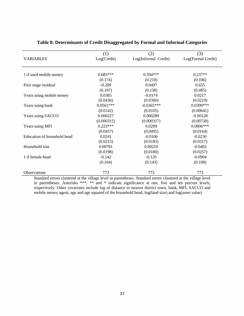
[ Insert Table 7 here ]We disaggregate the amount of credit received by the household into

formal and informal categories to investigate the two possible pathways through which

mobile money access could influence the credit behavior of the household. As noted before,

the first possible channel could be the facilitation of informal borrowing arrangements among

family members, friends, individual money lenders and members of local savings and credit

associations made possible by the availability of a convenient remittance channel. The second

channel is rather less straightforward; the recent interlinkage between mobile network

operators and banking institutions – commercial banks and MFIs – allowed for the

interconnectivity of mobile money accounts and bank accounts. This innovation allows users

to freely move funds between the two types of accounts and could have made it swifter for

banking institutions to market their loan products to mobile money users through short

messaging service (SMS) and disseminate loan proceeds to borrowers without requiring them

to physically travel to bank branches. It is also possible that the interlinkage could have

increased service satisfaction among customers using interlinked bank and mobile money

accounts, increasing their demand for loan products. Results in Columns 3 and 4 of Table 8

confirm that both pathways are at play; both informal and formal credit increases with mobile

money possession. However, as noted earlier, the informal channel is stronger, indicating the

20

ease associated with mobile money in exchanging informal microcredit among members of

informal social networks and private money lenders.

[ Insert Table 8 here ]

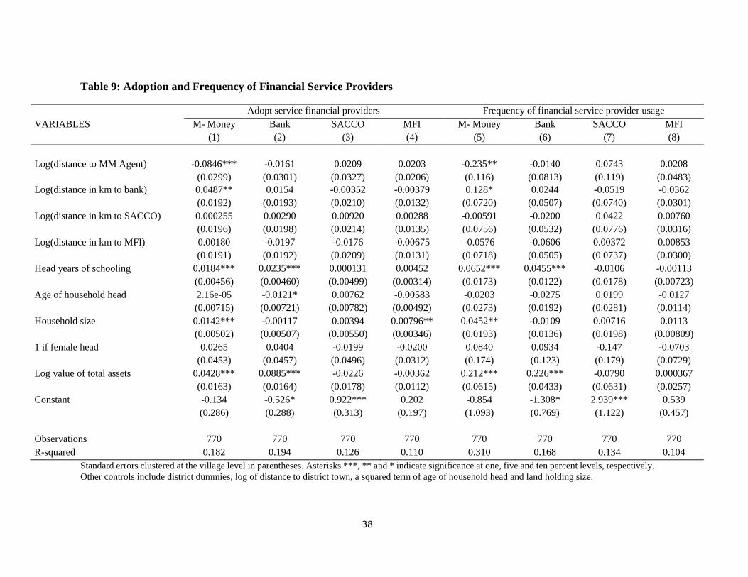
5.3. Mechanisms: Usage Financial Service Providers.

Table 9 presents estimation results from a system of seemingly unrelated regressions that

take into account potentially interdependence in household’s decisions to adopt the four

financial service providers – mobile money, bank, SACCO and MFI. For each of the four

financial service providers, the dependent variables in Columns 1 to 4 are binary indicators

taking one if the household used the respective service provider within a year preceding the

survey while the frequency of using the service providers is presented in Columns 5 to 8.

Columns 1 and 4 respectively reveal that the probability of using mobile money services

reduces by eight percentage points and 24 percent when the distance from the village center

to the nearest mobile money agent doubles. Distances to the nearest bank, SACCO and MFI

do not significantly enter into the household decision to adopt these institutions. One possible

explanation in the case of bank adoption is that no matter how close the household may be

to the bank premises, sign-up documentation as well as actual and/or perceived cost of

account opening and maintenance may impose additional restrictions to the up-take of bank

accounts. The significantly positive coefficient on log of asset value rather stresses the

relative importance of household wealth, implying that asset-wealthy households can afford

to use bank services despite the long distances they have to travel to access these services.

The education level of the household head is positively associated with a higher likelihood

21

and frequency of using mobile money and banks, which may reflect the literacy role in

shaping financial behavior.

[ Insert Table 9 here ]

5.4. Robustness checks.

5.4.1. Endogeneity of mobile money adoption.

In all previous results, we treated mobile money adoption as exogenous to the

household. However, this is unlikely because households who normally save or borrow

money and receive remittances may adopt mobile money services to ease the flow of these

services. In this case, causation runs in the reverse direction and this implies potential

endogeneity of mobile money adoption due to simultaneous effects. The default approach in

this case would be to run instrumental variable regressions in a 2SLS framework using

distance to the mobile money agent as an instrument for mobile money adoption. We instead

add a control function approach to our Tobit models to establish a causal link between mobile

money adoption and financial service amounts while taking into account the corner solution

problem in our outcome variables.13 In the first step, we run probit models for mobile money

adoption on all exogenous variables including log of distance to the nearest mobile money

agent (results not shown) and obtain predicted residuals which we add as an extra covariate

in the (second-step) outcome regressions. The results reported in the odd-numbered columns

of Table 4 show that the mobile money coefficient remains strongly significant. The positive

13 From this point throughout the analysis that follows, we refer to this approach as Tobit-CF.

22

coefficient on the predicted residuals in savings and credit regressions indicates that the

endogeneity of mobile money imposed an upward bias on our Tobit estimates of these

variables. Luckily, the inclusion of auxiliary residuals in our Tobit models not only checks

for endogeneity but also alleviates its confounding power (Wooldridge, 2003; Mason, 2013).

5.4.2. Alternative Explanations.

We presume that the distance to the mobile money agent is independent of household and

village characteristics because mobile money agents were, in most cases, already established

shop keepers in the villages selling household merchandize and airtime cards, who later took

on mobile money as an additional service on their service menus when this financial platform

was introduced in the country in 2009. This differs from the case where non-resident mobile

money entrepreneurs self-select into the villages they perceive to be profitable. Nonetheless,

we appreciate the possibility that already established shop keepers could decide whether or

not to extend their range of services to cover mobile money, basing on the local economic

potential of villages, which could be a reflection of potential demand from the residents. A

profit-oriented mobile money agent would consider the local economic potential of the

village and locate in the village town, which is often closer to the district headquarters

(district town). However, we control for distance from the village center to the nearest district

town in all our regressions and our estimates remain qualitatively and quantitatively similar

to those without this control (unreported).

The second concern relates to the possibility that banks, SACCOs and MFIs could

have mobilized savings and credit during or prior to our study period. If this was the case,

23

our estimates would be capturing the spurious correlation between mobile money adoption

and the up-take of financial services. However, for 90 percent of our sample villages, the

nearest banks and MFIs are available in the district town and controlling for this distance

provides a remedy to this problem. It is important to note, however, that SACCOs are

available in most villages and the distance to the district town does not necessarily affect

their power to infiltrate and mobilize financial service up-take among rural households. We

therefore control for the distance to the nearest SACCO, a dummy variable for household

membership to SACCOs and binary indicators for whether a SACCO is present in the village

in Tables 4, 5 and 6 and our results remain highly robust14.

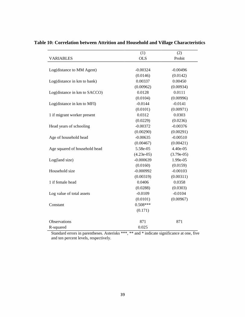
5.4.3. Attrition

The final check for the robustness of our results is a test for the possibility of attrition bias.

As discussed in earlier sections, we were able to follow 820 out the 916 households that were

sampled in the fourth round of RePEAT in 2012. This represents a 10.5 percent attrition rate

which could bias our results if the households that could not be interviewed in 2014

systematically differ from those that were successfully interviewed. We therefore regress the

attrition indicator on key household and village characteristics and show OLS and Probit

results respectively in Columns 1 and 2 of Table 10. The results reveal no systematic

differences between households that were interviewed in 2014 and those that were missed,

suggesting that attrition bias does not confound our main results.

14 We control for these variables separately due to collinearity. However, we report only results with distance to SACCO and district town to save space. Moreover, results were qualitatively similar across all specifications.

24

6. Conclusion

As lack of access to financial services remains a key challenge to many people in developing

countries, the advent of mobile phone-based financial platforms has been changing the

financial livelihoods of the rural poor. Mobile money – a financial innovation that allows the

user to deposit, exchange and withdraw money using their mobile phone – is a cheap and

convenient option for majority of the financially excluded rural populace.

We explore the role of this financial product in shaping the financial behavior of rural

households in Uganda using a randomly selected sample of 820 households. We provide

empirical evidence that mobile money leverages the financial access constraint of rural

households and stimulates their uptake of financial services. Accounting for possible

selection bias, endogeneity of mobile money adoption at the household level and the

influence of local economic conditions at the village level, we provide robust evidence that

the amounts of remittances, credit and savings made by mobile money users is significantly

higher than that of non-users. Our results feed into existing literature in two ways; first, by

profiling the potential of mobile money to drive remittance flow and second, by illustrating

that reducing service cost and distance to service points improves the saving behavior of rural

households. This paper uniquely contributes to the literature by extending the analysis of the

potential of mobile money beyond the traditional peer-to-peer remittances to credit and

saving services.

We illustrate that the main mechanism of this observed effect is the reduction of

distance to service points, as mobile money agents are located in almost all the sub-counties

25

in our study areas. We therefore postulate that access to mobile money services reduces the

burden in terms of transport and time cost associated with remittance and informal credit

exchange among family members and friends and boosts temporary savings to facilitate

school fees and farm investments. The cross-sectional nature of our data, however, does not

allow us to rule out the potential effect of unobserved household fixed attributes that could

influence the observed financial behavior and we leave this issue for future research. In the

case of remittances, this concern was alleviated using household fixed effects models in

Munyegera and Matsumoto (forthcoming). Nonetheless, our results suggest a critical policy

implication that enhancing access to convenient and affordable financial services has a great

potential to boost financial access among the rural poor who are often excluded from the

formal financial system. This enhanced access could improve their financial behavior and

augment their capacity to smooth consumption, safeguard against vulnerabilities in their lives

and make productive investments, eventually redeeming themselves from poverty.

26

References

Aker, J. C., Boumnijel, R., McClelland, A., & Tierney, N. (2011). Zap it to me: the short-

term impacts of a mobile cash transfer program. Center for Global Development

working paper, (268).

Anzoategui, D., Demirgüç-Kunt, A., & Martínez Pería, M. S. (2014). Remittances and

Financial Inclusion: Evidence from El Salvador. World Development, 54, 338-349.

Appleyard, L. (2011). Community Development Finance Institutions (CDFIs): Geographies

of financial inclusion in the US and UK. Geoforum, 42(2), 250-258.

Arestis, P., & Demetriades, P. (1997). Financial development and economic growth:

assessing the evidence. The Economic Journal, 107(442), 783-799.

Beck, T., Demirgüç-Kunt, A., & Singer, D. (2013). Is small beautiful? financial structure,

size and access to finance. World Development, 52, 19-33.

Cameron, A.C., & Trivedi, P.K. (2009). Microeconometrics Using Stata, Texas: StataCorp

LP.

Christopoulos, D. K., & Tsionas, E. G. (2004). Financial development and economic growth:

evidence from panel unit root and cointegration tests. Journal of development

Economics, 73(1), 55-74.

Cracknell, D. (2004). Electronic banking for the poor–panacea, potential and pitfalls. Small

Enterprise Development, 15(4), 8-24.

27

de Lis, S. F., Llanes, M. C., Lopez-Moctezuma, C., Rojas, J. C., & Tuesta, D.

(2014). Financial inclusion and the role of mobile banking in Colombia.

Developments and potential (No. 1404).

Demirgüç-Kunt, A., & Klapper, L. F. (2012). Measuring financial inclusion: The global

findex database. World Bank Policy Research Working Paper, (6025).

Dupas, P. & Robinson, J. (2013). Savings Constraints and Microenterprise Development:

Evidence from a Field Experiment in Kenya American Economic Journal: Applied

Economics 2013, 5(1): 163–192

Honohan, P. (2008). Cross-country variation in household access to financial

services. Journal of Banking & Finance, 32(11), 2493-2500.

Hughes, N., & Lonie, S. (2007). M-PESA: mobile money for the “unbanked” turning

cellphones into 24-hour tellers in Kenya. Innovations, 2(1-2), 63-81.

Imbens, G. M., & Wooldridge, J. M. (2008). Recent developments in the econometrics of

program evaluation (No. w14251). National Bureau of Economic Research.

Jack, W., & Suri, T. (2014). Risk Sharing and Transactions Costs: Evidence from Kenya's

Mobile Money Revolution. The American Economic Review,104(1), 183-223.

Jack, W., Ray, A., Suri, T. (2013). Transaction Networks: Evidence from Mobile Money in

Kenya. American Economic Review, 103(3), 356-61.

Jack, W., Suri, T. (2011). Risk sharing and transaction costs: Evidence from Kenya’s mobile

money revolution’. Working paper.

28

Jalilian, H., & Kirkpatrick, C. (2005). Does financial development contribute to poverty

reduction?. Journal of Development Studies, 41(4), 636-656.

Johnson, S., & Nino-Zarazua, M. (2011). Financial access and exclusion in Kenya and

Uganda. The Journal of Development Studies, 47(3), 475-496.

Kikulwe, E. M., Fischer, E., & Qaim, M. (2013). Mobile money, market transactions, and

household income in rural Kenya (No. 22). GlobalFood Discussion Papers.

King, R. G., & Levine, R. (1993). Finance, entrepreneurship and growth. Journal of

Monetary economics, 32(3), 513-542.

King, R. G., & Levine, R. (1993). Finance and growth: Schumpeter might be right. The

quarterly journal of economics, 717-737.

Levine, R. (1997). Financial development and economic growth: views and agenda. Journal

of economic literature, 688-726.

Morawczynski, O., & Pickens, M. (2009). Poor people using mobile financial services:

observations on customer usage and impact from M-PESA.

Munyegera, G. K., & Matsumoto, T. (Forthcoming). Mobile Money, Remittances and Rural

Household Welfare: Panel Evidence from Uganda, World Development.

Odhiambo, N. M. (2009). Financial deepening and poverty reduction in Zambia: an empirical

investigation. International Journal of Social Economics, 37(1), 41-53.

Patrick, H. T. (1966). Financial development and economic growth in underdeveloped

countries. Economic development and Cultural change, 174-189.

29

Pedrosa, J., & Do, Q. (2011). Geographic Distance and Credit Market Access in

Niger. African Development Review/Revue Africaine De Developpement, 23(3), 289-

299.

Rosenbaum, P. R., & Rubin, D. B. (1985). Constructing a control group using multivariate

matched sampling methods that incorporate the propensity score.The American

Statistician, 39(1), 33-38.

Swamy, V. (2014). Financial Inclusion, Gender Dimension, and Economic Impact on Poor

Households. World Development, 56, 1-15.

30

Table 1: Access to and Usage of Financial Services by Mobile Money Adoption Status in 2014

Non-adopters Adopters Difference VARIABLES Mean SD Mean SD Mean Usage of financial services

1 if saved money in past 12 months 0.56 0.50 0.80 0.39 0.24***

1 if borrowed money in past 12 months 0.48 0.50 0.69 0.46 0.21***

Amount saved in past 12 months (1,000 UGX) 196 431 664 1,415 468***

Amount borrowed in past 12 months (1,000 UGX) 138 305 619 1,248 481***

1 if owns bank account 0.13 0.32 0.41 0.49 0.28***

1 if belongs to SACCO 0.53 0.49 0.65 0.47 0.12***

1 if used an MFI 0.02 0.14 0.10 0.34 0.08***

1 if received remittance 0.62 0.48 0.72 0.44 0.10***

Total value of remittances (1,000 UGX) 325 826 702 1,350 377***

Access to financial services

1 if bank available in LC1 0.06 0.23 0.12 0.32 0.06**

1 if mobile money agent available in LC1 0.35 0.47 0.48 0.49 0.13***

1 if MFI available in LC1 0.08 0.26 0.10 0.29 0.02

1 if SACCO available in LC1 0.56 0.49 0.61 0.48 0.05

Distance from LC1 to nearest bank 54.84 87.72 53.20 85.88 1.64

Distance from LC1 to nearest MM Agent (km) 4.73 4.10 3.76 3.88 0.97***

Distance from LC1 to nearest MFI (km) 27.31 29.28 23.84 27.52 -3.47

Distance from LC1 to nearest SACCO (km) 5.86 10.76 6.16 11.64 0.30

Observations 242 574

Note: Authors’ Computation based on RePEAT4 and MM2014.The average exchange rate during the survey period was UGX 2,600 per USD 1(Bank of Uganda, 2014). Asterisks ***, ** and * indicate significance of mean difference at one, five and ten percent levels, respectively.

31

Table 2: Household and Village Characteristics by Mobile Money Adoption Status in 2014

Non-adopters Adopters Difference VARIABLES Mean SD Mean SD Mean Household characteristics

1 if owns any mobile phone 0.54 0.49 0.89 0.31 0.35***

Total value of assets (1,000 UGX) 681 1,344 1,236 2,126 555***

Land size (hectare) 5.02 5.51 6.91 8.75 1.89***

Household size 6.26 3.29 7.33 3.47 1.07***

Age of household head 52.83 15.32 51.64 13.57 -1.19

1 if female head 0.17 0.38 0.14 0.35 0.03

Head years of schooling 4.40 3.49 6.48 3.84 2.08***

Village characteristics

Distance (km) from LC1 to nearest district town 11.03 0 .56 9.86 0 .36 1.16*

Observations 242 574

Note: Authors’ Computation based on RePEAT4 and MM2014.The average exchange rate during the survey period was UGX 2,600 per USD 1(Bank of Uganda, 2014). Asterisks ***, ** and * indicate significance of mean difference at one, five and ten percent levels, respectively.

32

Table 3: Determinants of Financial Service Usage: Marginal Effects from Probit Regression

Pr(Savings=1) Pr(Credit=1) Pr(Remittance=1)

VARIABLES (1) (2) (3) (4) (5) (6)

1 if used mobile money 0.249*** 0.220*** 0.815***

(0.0407) (0.0426) (0.0298)

Log(distance to MM Agent) -0.0213 0.0284 -0.0457*

(0.0273) (0.0306) (0.0272)

Education of household head 0.00671 0.0112** 0.00472 0.00994* 0.000236 0.0176***

(0.00500) (0.00486) (0.00538) (0.00530) (0.00595) (0.00508)

Age of household head 0.00523 0.00631 0.0118 0.0106 -0.0154** -0.0105

(0.00763) (0.00748) (0.00882) (0.00904) (0.00723) (0.00753)

Household size -0.00525 -0.00210 0.00118 0.00405 0.0133** 0.0186***

(0.00535) (0.00535) (0.00592) (0.00591) (0.00569) (0.00585)

1 if female head 0.0149 0.0248 -0.0517 -0.0409 -0.0577 -0.0127

(0.0464) (0.0450) (0.0539) (0.0530) (0.0472) (0.0475)

Log(total asset value) 0.0249 0.0345* -0.0109 -0.000317 0.0494** 0.0655***

(0.0181) (0.0178) (0.0191) (0.0187) (0.0194) (0.0179)

Observations

Pseudo R-Squared

785

0.124

785

0.083

785

0.090

785

0.066

785

0.654

785

0.191

Standard errors clustered at the village level in parentheses. Standard errors clustered at the village level in parentheses. Asterisks ***, ** and * indicate significance at one, five and ten percent levels, respectively. Included controls not shown in the table include district dummies. A mobile money dummy is used as a poxy for access to mobile money services in odd-numbered columns. In even-numbered columns, mobile money access is measured by physical distance to the nearest mobile money agent.

33

Table 4: Amount (in log) of Remittances, Credit and Savings: Tobit Model with CF and full Controls Log(Savings Amount) Log(Credit Amount) Log(Remittance Amount) VARIABLES (1) (2) (3) (4) (5) (6) 1 if used mobile money 0.817*** 0.820*** 0.685*** 0.654*** 0.840** 0.766** (0.234) (0.251) (0.123) (0.133) (0.364) (0.387) First stage residual 1.517** 0.650* -0.604 (0.671) (0.368) (1.044) Log(Distance to district town) -0.0554 -0.0509 -0.0277 -0.0205 -0.170 -0.138 (0.154) (0.154) (0.0964) (0.0969) (0.284) (0.284) 1 if migrant worker present 0.0620 0.00338 -0.217 -0.236* 0.750** 0.775** (0.235) (0.236) (0.142) (0.142) (0.355) (0.361) 1 if SACCO available in LC1 0.117 0.127 0.0110 0.0135 0.377 0.421 (0.267) (0.268) (0.160) (0.161) (0.413) (0.414) Head years of schooling 0.0329 0.00728 0.0308* 0.0191 0.0351 0.0461 (0.0292) (0.0310) (0.0184) (0.0197) (0.0448) (0.0478) Age of household head 0.0129 0.0127 -0.00335 -0.00220 -0.0160 -0.00632 (0.0473) (0.0475) (0.0290) (0.0291) (0.0690) (0.0691) Log value of land currently held 0.0674 -0.00721 0.0348 -0.00304 0.491* 0.527* (0.170) (0.174) (0.106) (0.107) (0.265) (0.271) Household size -0.0664* -0.0854** -0.00351 -0.0140 -0.0392 -0.0321 (0.0346) (0.0361) (0.0188) (0.0196) (0.0507) (0.0519) 1 if female head -0.311 -0.327 -0.211 -0.222 1.122*** 1.101*** (0.306) (0.308) (0.163) (0.164) (0.411) (0.412) Log value of total assets 0.190* 0.140 0.114* 0.0937 0.993*** 1.011*** (0.112) (0.113) (0.0633) (0.0652) (0.158) (0.160) Observations 770 770 770 770 770 770

Standard errors clustered at the village level in parentheses. Asterisks ***, ** and * indicate significance at one, five and ten percent levels,

respectively. Included controls not shown in the table include district dummies and a squared term of age of household head and land holding

size.

34

Table 5: Adoption and Amount of Financial Services: Marginal Effects from Reduced Form Tobit

Pr(Saving=1) Log(Savings Amount)

Pr(Credit=1) Log(Credit Amount)

Pr(Remit=1) Log(Remit Amount)

VARIABLES (1) (2) (3) (4) (5) (6) Log(distance to MM Agent) -0.0547* -0.371** -0.0278* -0.143* -0.0814** -0.328** (0.0319) (0.181) (0.0253) (0.0863) (0.0337) (0.141) Log(distance in km to bank) 0.0387 0.238 0.0294* 0.0719 0.0492** 0.233** (0.0217) (0.124) (0.0173) (0.0570) (0.0244) (0.109) Log(distance in km to SACCO) -0.00990 -0.0544 0.00161 -0.0398 0.00789 -0.0321 (0.0217) (0.130) (0.0182) (0.0635) (0.0236) (0.0937) Log(distance in km to MFI) -0.00398 -0.0129 -0.0228 -0.0287 -0.00170 0.00445 (0.0216) (0.123) (0.0182) (0.0631) (0.0235) (0.103) Head years of schooling 0.00880* 0.0670** 0.00516 0.0376** 0.0154*** 0.0974*** (0.00514) (0.0295) (0.00503) (0.0180) (0.00566) (0.0231) Age of household head 0.00268 0.0150 0.000982 -0.0123 -0.0107 -0.0384 (0.00805) (0.0498) (0.00848) (0.0299) (0.00864) (0.0366) Household size -0.00565 -0.0427 0.00390 0.000409 0.0146** 0.0592** (0.00559) (0.0359) (0.00560) (0.0195) (0.00603) (0.0253) 1 if female head -0.0212 -0.266 -0.0562 -0.195 -0.0314 -0.225 (0.0508) (0.311) (0.0513) (0.167) (0.0520) (0.210) Log value of total assets 0.0365* 0.260** 0.00211 0.163*** 0.0469** 0.310*** (0.0187) (0.112) (0.0175) (0.0622) (0.0192) (0.0821) Observations 784 784 784 784 784 784

Standard errors clustered at the village level in parentheses. Asterisks ***, ** and * indicate significance at one, five and ten percent levels, respectively. Other controls include district dummies, log of distance to district town, a squared term of age of household head and land holding size.

35

Table 6: Weighted Regression Analysis Based on Propensity Score

Pr(Savings=1) Log(Savings) Pr(Credit=1) Log(Credit) Pr(Remit=1) Log(Remittance) VARIABLES (1) (2) (3) (4) (5) (6) 1 if used mobile money 0.172*** 0.534*** 0 .140** 0.680*** 0 .637*** 0.639** (0.054) (0.168) (0 .055) (0.127) (0 .038) (0.321) Head years of schooling 0.005 0.0507 0.009 0.0611** -0.00002 0.0456 (0.006) (0.0327) (0.006) (0.0251) (0.005) (0.0292) Age of household head 0.001 0.00246 0.003 -0.00531 -0.011 -0.0167 (0.008) (0.0422) (0.008) (0.0353) (0.005) (0.0345) Household size -0.002 -0.0369 0.0006 -0.0114 0.002 0.0332 (0 .006) (0.0352) (0.007) (0.0264) (0.004) (0.0311) 1 if female head -0.019 -0.168 -0.046 -0.177 -0.079 0.347 (0.051) (0.280) (0.054) (0.206) (0.040) (0.259) Log(distance to MM Agent) -0.034 -0.253 0.032 0.165 -0.002 0.0739 (0.034) (0.190) (0.036) (0.145) (0.025) (0.179) Log(distance in km to bank) 0.026 0.170 0.018 0.0602 0.021 0.195* (0.022) (0.121) (0.023) (0.0903) (0.016) (0.111) Log(distance in km to SACCO) -0.008 -0.0727 0.003 0.0128 0.016 0.117 (0.022) (0.129) (0.024) (0.100) (0.015) (0.107) Log(distance in km to MFI) -0.006 0.0160 -0.029 -0.101 -0.028 -0.167 (0.021) (0.119) (0.023) (0.0925) (0.015) (0.105) Log(Distance in km to district town) -0.008 -0.0933 0.022 0.0501 0.043 0.259 (0.031) (0.168) (0.035) (0.139) (0.024) (0.160) Log value of total assets 0.040** 0.235** -0.003 0.117 0.003 0.0121 (0.018) (0.111) (0.020) (0.0905) (0.014) (0.0987) Observations 673 673 673 673 673 673 R-squared 0.158 0.200 0.124 0.196 0.550 0.258

Standard errors clustered at the village level in parentheses. Asterisks ***, ** and * indicate significance at one, five and ten percent levels, respectively. Additional controls include landholding size, a dummy for the presence of a migrant worker and district dummies.

36

Table 7: Balance Check for Comparability of Covariates before and after Propensity Score Matching

Mean before Mean after % |Bias|

Variables MM=1 MM=0 P-value MM=1 MM=0 P-value Reduction

Head years of schooling 5.79 4.12 0.000 5.94 5.96 0.889 89.6

Age of household head 51.39 52.52 0.326 51.39 50.22 0.194 63.7

Land size in hectares 5.83 4.51 0.005 5.83 5.48 0.342 78.4

Household size 6.93 6.15 0.002 6.93 6.86 0.731 91.3

1 if female head 0.15 0.19 0.25 0.15 0.13 0.466 50.8

Total assets in 1,000 UGX 850 550 0.000 850 800 0.400 63.2

Distance in km to MM agent 4.14 4.86 0.030 4.14 4.14 0.989 99.5

Distance in km to bank 54.24 56.47 0.756 54.24 50.16 0.462 83.0

Distance in km to SACCO 6.12 6.05 0.938 6.12 5.49 0.388 74.8

Distance in km to MFI 23.70 27.79 0.074 23.75 23.16 0.444 85.3

Distance in km to district town 10.41 11.34 0.200 10.41 10.40 0.990 99.2

1 if owns mobile phone 0.82 0.51 0.000 0.82 0.81 0.279 96.8

Pseudo R2 - - 0.077 - - 0.006 -

Mean Bias - - 16.9 - - 3.4 -

P-value (Joint Mean Equality) - - 0.000 - - 0.724 -

Balance check before and after PSM for observations for which 0.1<e(X)<0.9. Pseudo R2 indicates how well covariates explain treatment probability; a small value after matching indicates goodness of the matching technique (Sianesi, 2004). A standardized absolute mean bias less than 5 after matching indicates effective matching (Rosenbaum and Rubin, 1985). A non-significant p-value for the joint mean equality test after matching shows significant similarity between treatment and control groups after matching (Caliendo & Kopeinig, 2008).

37

Table 8: Determinants of Credit Disaggregated by Formal and Informal Categories

(1) (2) (3) VARIABLES Log(Credit) Log(Informal Credit) Log(Formal Credit)

1 if used mobile money 0.685*** 0.594*** 0.237** (0.174) (0.218) (0.106) First stage residual -0.289 0.0497 0.655 (0.187) (0.158) (0.485) Years using mobile money 0.0385 -0.0174 0.0217 (0.0436) (0.0360) (0.0219) Years using bank 0.0561*** -0.0365*** 0.0399*** (0.0142) (0.0105) (0.00641) Years using SACCO 0.000227 0.000289 -0.00128 (0.000315) (0.000317) (0.00738) Years using MFI 0.223*** 0.0299 0.0806*** (0.0457) (0.0495) (0.0164) Education of household head 0.0241 -0.0106 -0.0230 (0.0215) (0.0183) (0.0317) Household size 0.00781 0.00210 -0.0402 (0.0198) (0.0180) (0.0257) 1 if female head -0.142 -0.120 -0.0904 (0.164) (0.143) (0.108) Observations 773 773 773

Standard errors clustered at the village level in parentheses. Standard errors clustered at the village level in parentheses. Asterisks ***, ** and * indicate significance at one, five and ten percent levels, respectively. Other covariates include log of distance to nearest district town, bank, MFI, SACCO and mobile money agent; age and age squared of the household head; log(land size) and log(asset value)

38

Table 9: Adoption and Frequency of Financial Service Providers

Adopt service financial providers Frequency of financial service provider usage VARIABLES M- Money Bank SACCO MFI M- Money Bank SACCO MFI (1) (2) (3) (4) (5) (6) (7) (8) Log(distance to MM Agent) -0.0846*** -0.0161 0.0209 0.0203 -0.235** -0.0140 0.0743 0.0208 (0.0299) (0.0301) (0.0327) (0.0206) (0.116) (0.0813) (0.119) (0.0483) Log(distance in km to bank) 0.0487** 0.0154 -0.00352 -0.00379 0.128* 0.0244 -0.0519 -0.0362 (0.0192) (0.0193) (0.0210) (0.0132) (0.0720) (0.0507) (0.0740) (0.0301) Log(distance in km to SACCO) 0.000255 0.00290 0.00920 0.00288 -0.00591 -0.0200 0.0422 0.00760 (0.0196) (0.0198) (0.0214) (0.0135) (0.0756) (0.0532) (0.0776) (0.0316) Log(distance in km to MFI) 0.00180 -0.0197 -0.0176 -0.00675 -0.0576 -0.0606 0.00372 0.00853 (0.0191) (0.0192) (0.0209) (0.0131) (0.0718) (0.0505) (0.0737) (0.0300) Head years of schooling 0.0184*** 0.0235*** 0.000131 0.00452 0.0652*** 0.0455*** -0.0106 -0.00113 (0.00456) (0.00460) (0.00499) (0.00314) (0.0173) (0.0122) (0.0178) (0.00723) Age of household head 2.16e-05 -0.0121* 0.00762 -0.00583 -0.0203 -0.0275 0.0199 -0.0127 (0.00715) (0.00721) (0.00782) (0.00492) (0.0273) (0.0192) (0.0281) (0.0114) Household size 0.0142*** -0.00117 0.00394 0.00796** 0.0452** -0.0109 0.00716 0.0113 (0.00502) (0.00507) (0.00550) (0.00346) (0.0193) (0.0136) (0.0198) (0.00809) 1 if female head 0.0265 0.0404 -0.0199 -0.0200 0.0840 0.0934 -0.147 -0.0703 (0.0453) (0.0457) (0.0496) (0.0312) (0.174) (0.123) (0.179) (0.0729) Log value of total assets 0.0428*** 0.0885*** -0.0226 -0.00362 0.212*** 0.226*** -0.0790 0.000367 (0.0163) (0.0164) (0.0178) (0.0112) (0.0615) (0.0433) (0.0631) (0.0257) Constant -0.134 -0.526* 0.922*** 0.202 -0.854 -1.308* 2.939*** 0.539 (0.286) (0.288) (0.313) (0.197) (1.093) (0.769) (1.122) (0.457) Observations 770 770 770 770 770 770 770 770 R-squared 0.182 0.194 0.126 0.110 0.310 0.168 0.134 0.104

Standard errors clustered at the village level in parentheses. Asterisks ***, ** and * indicate significance at one, five and ten percent levels, respectively. Other controls include district dummies, log of distance to district town, a squared term of age of household head and land holding size.

39

Table 10: Correlation between Attrition and Household and Village Characteristics

(1) (2) VARIABLES OLS Probit Log(distance to MM Agent) -0.00324 -0.00496 (0.0146) (0.0142) Log(distance in km to bank) 0.00337 0.00450 (0.00962) (0.00934) Log(distance in km to SACCO) 0.0128 0.0111 (0.0104) (0.00996) Log(distance in km to MFI) -0.0144 -0.0141 (0.0101) (0.00971) 1 if migrant worker present 0.0312 0.0303 (0.0229) (0.0236) Head years of schooling -0.00372 -0.00376 (0.00290) (0.00291) Age of household head -0.00635 -0.00510 (0.00467) (0.00421) Age squared of household head 5.58e-05 4.40e-05 (4.23e-05) (3.79e-05) Log(land size) -0.000639 1.99e-05 (0.0160) (0.0159) Household size -0.000992 -0.00103 (0.00319) (0.00311) 1 if female head 0.0406 0.0358 (0.0288) (0.0303) Log value of total assets -0.0109 -0.0104 (0.0101) (0.00967) Constant 0.508*** (0.171) Observations 871 871 R-squared 0.025 Standard errors in parentheses. Asterisks ***, ** and * indicate significance at one, five and ten percent levels, respectively.