Embed Size (px)
Citation preview

ICORD 2007, Brussels
Methodological Issues on Clinical Trials with Small Sample Size
Joachim Gerß, Wolfgang Köpcke
Department of Medical Informatics and Biomathematics, Münster, Germany
2
Outline
1. The innovative drug development approaches-project
2. Weakness of small sample trials
3. Increase the efficiency of statistical data analyses
3.1 Overview of methodologic approaches
3.2 Resampling
3.3 Repeated measurement designs
3.4 Bayesian models
4. Software
5. Summary and Conclusion
3
Outline
1. The innovative drug development approaches-project
2. Weakness of small sample trials
3. Increase the efficiency of statistical data analyses
3.1 Overview of methodologic approaches
3.2 Resampling
3.3 Repeated measurement designs
3.4 Bayesian models
4. Software
5. Summary and Conclusion
41. Innovative drug development approaches
INNOVATIVE DRUG DEVELOPMENT APPROACHES
FINAL REPORT FROM THE EMEA/CHMP-THINK-TANK GROUP ONINNOVATIVE DRUG DEVELOPMENT
Doc. Ref. EMEA/127318/2007
51. Innovative drug development approaches
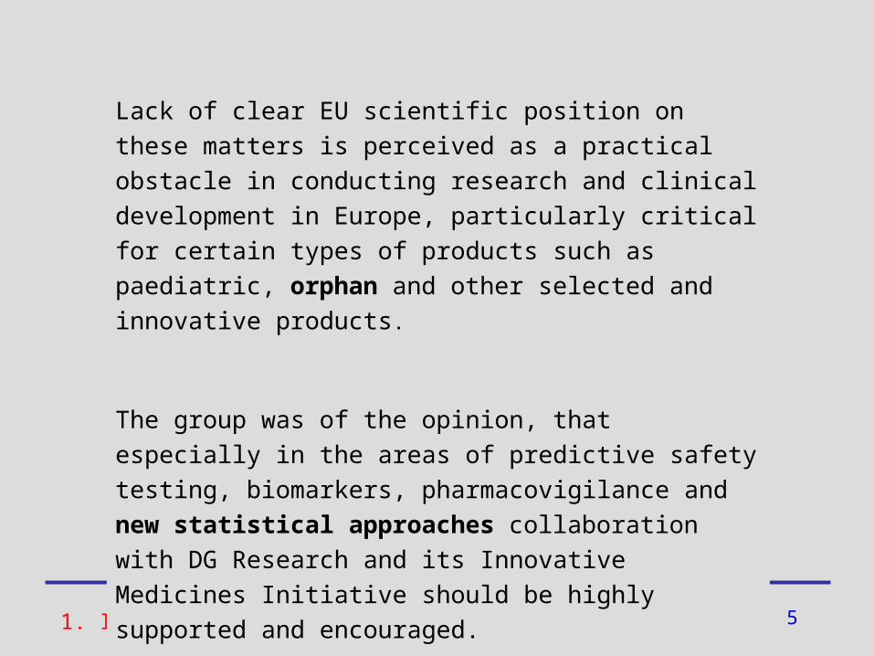
Lack of clear EU scientific position on these matters is
perceived as a practical obstacle in conducting research
and clinical development in Europe, particularly critical for
certain types of products such as paediatric, orphan and
other selected and innovative products.
The group was of the opinion, that especially in the areas of
predictive safety testing, biomarkers, pharmacovigilance
and new statistical approaches collaboration with DG
Research and its Innovative Medicines Initiative should be
highly supported and encouraged.
6
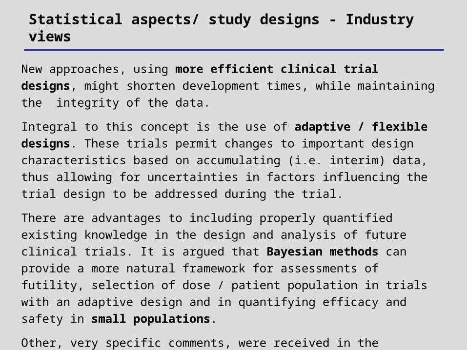
Statistical aspects/ study designs - Industry views
New approaches, using more efficient clinical trial designs, might shorten
development times, while maintaining the integrity of the data.
Integral to this concept is the use of adaptive / flexible designs. These trials
permit changes to important design characteristics based on accumulating (i.e.
interim) data, thus allowing for uncertainties in factors influencing the trial design
to be addressed during the trial.
There are advantages to including properly quantified existing knowledge in the
design and analysis of future clinical trials. It is argued that Bayesian methods
can provide a more natural framework for assessments of futility, selection of
dose / patient population in trials with an adaptive design and in quantifying
efficacy and safety in small populations.
Other, very specific comments, were received in the following areas: discontinue
the preference for / reliance on Last Observation Carried Forward (LOCF) for
imputation of missing data; increase the use of longitudinal methods rather
than analyses at single time points.
7
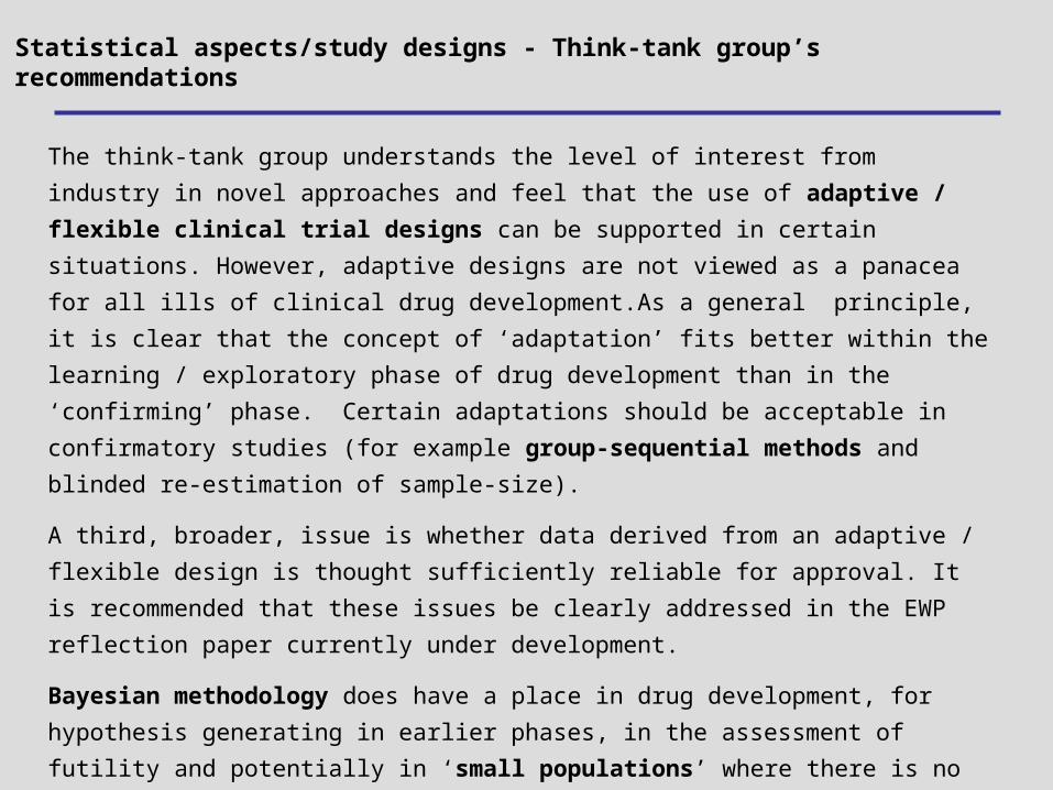
Statistical aspects/study designs - Think-tank group’s recommendations
The think-tank group understands the level of interest from industry in novel approaches
and feel that the use of adaptive / flexible clinical trial designs can be supported in
certain situations. However, adaptive designs are not viewed as a panacea for all ills of
clinical drug development.As a general principle, it is clear that the concept of ‘adaptation’
fits better within the learning / exploratory phase of drug development than in the
‘confirming’ phase. Certain adaptations should be acceptable in confirmatory studies (for
example group-sequential methods and blinded re-estimation of sample-size).
A third, broader, issue is whether data derived from an adaptive / flexible design is thought
sufficiently reliable for approval. It is recommended that these issues be clearly addressed
in the EWP reflection paper currently under development.
Bayesian methodology does have a place in drug development, for hypothesis generating
in earlier phases, in the assessment of futility and potentially in ‘small populations’ where
there is no possibility to perform an adequately powered randomised controlled trial.
However, with regards the use of ‘Bayesian’ methodology in confirmatory clinical trials, at
present the think-tank group does not recommend the use of informative priors in Phase III
trials, which should provide stand-alone, confirmatory evidence of efficacy and safety.
8
Outline
1. The innovative drug development approaches-project
2. Weakness of small sample trials
3. Increase the efficiency of statistical data analyses
3.1 Overview of methodologic approaches
3.2 Resampling
3.3 Repeated measurement designs
3.4 Bayesian models
4. Software
5. Summary and Conclusion
9
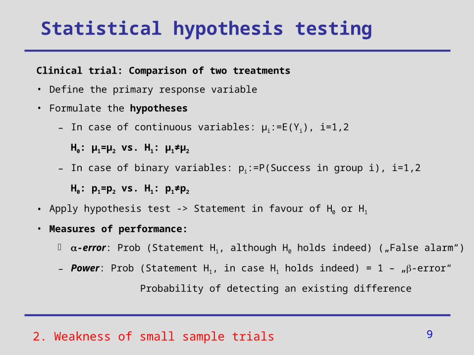
Statistical hypothesis testing
Clinical trial: Comparison of two treatments
• Define the primary response variable
• Formulate the hypotheses
– In case of continuous variables: µi:=E(Yi), i=1,2
H0: µ1=µ2 vs. H1: µ1≠µ2
– In case of binary variables: pi:=P(Success in group i), i=1,2
H0: p1=p2 vs. H1: p1≠p2
• Apply hypothesis test -> Statement in favour of H0 or H1
• Measures of performance:
-error: Prob (Statement H1, although H0 holds indeed) („False alarm“)
– Power: Prob (Statement H1, in case H1 holds indeed) = 1 – „-error“
Probability of detecting an existing difference
2. Weakness of small sample trials
10
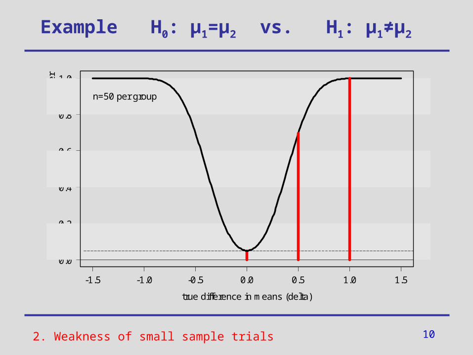
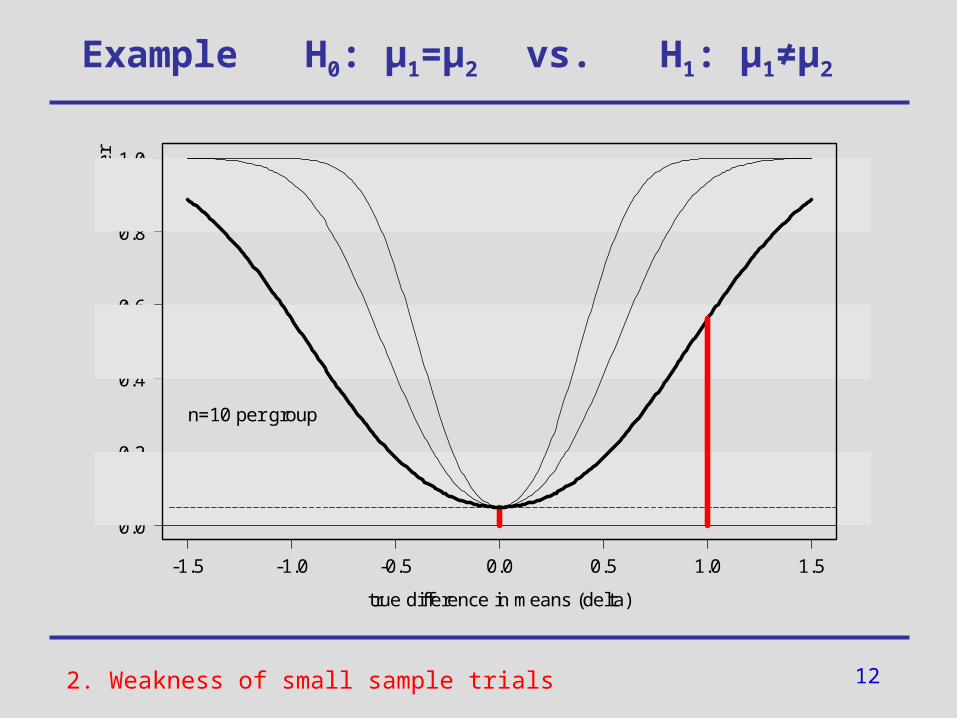
Example H0: µ1=µ2 vs. H1: µ1≠µ2
-1.5 -1.0 -0.5 0.0 0.5 1.0 1.5
0.0
0.2
0.4
0.6
0.8
1.0
true difference in means (delta)
Pow
er
n=50 per group
2. Weakness of small sample trials
11
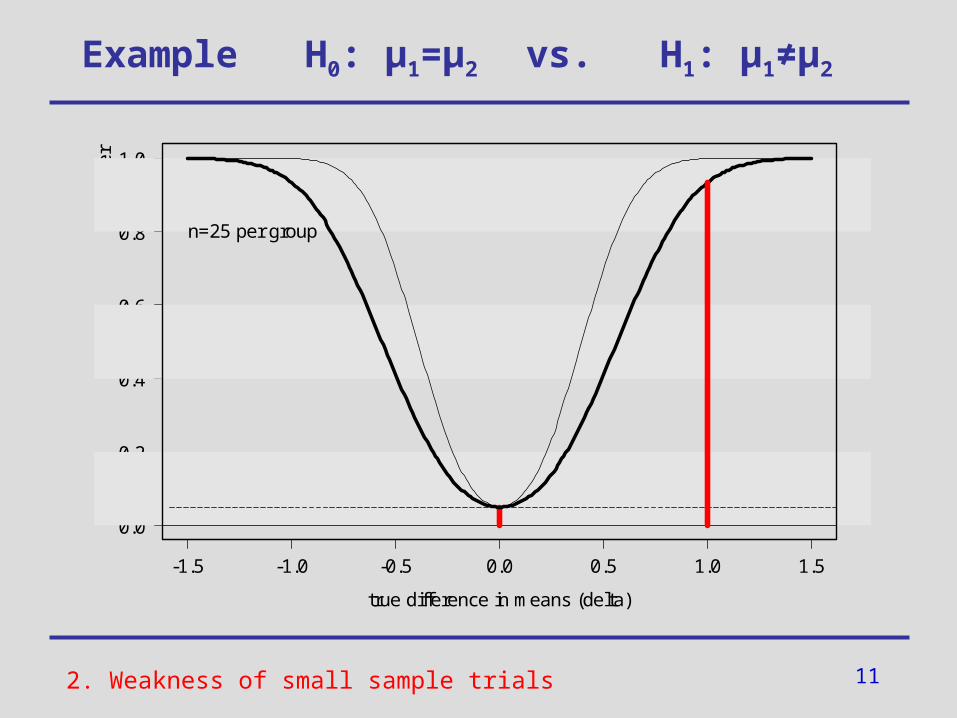
Example H0: µ1=µ2 vs. H1: µ1≠µ2
-1.5 -1.0 -0.5 0.0 0.5 1.0 1.5
0.0
0.2
0.4
0.6
0.8
1.0
true difference in means (delta)
Pow
er
n=25 per group
2. Weakness of small sample trials
12
Example H0: µ1=µ2 vs. H1: µ1≠µ2
-1.5 -1.0 -0.5 0.0 0.5 1.0 1.5
0.0
0.2
0.4
0.6
0.8
1.0
true difference in means (delta)
Pow
er
n=10 per group
2. Weakness of small sample trials
13
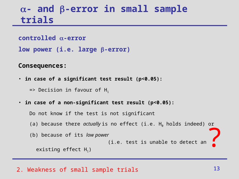
controlled -error
low power (i.e. large -error)
Consequences:
• in case of a significant test result (p<0.05):
=> Decision in favour of H1
• in case of a non-significant test result (p<0.05):
Do not know if the test is not significant
(a) because there actually is no effect (i.e. H0 holds indeed) or
(b) because of its low power (i.e.
test is unable to detect an existing effect H1)
- and -error in small sample trials
?2. Weakness of small sample trials
14
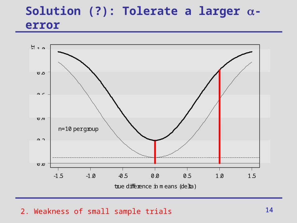
Solution (?): Tolerate a larger -error
-1.5 -1.0 -0.5 0.0 0.5 1.0 1.5
0.0
0.2
0.4
0.6
0.8
1.0
true difference in means (delta)
Pow
er
n=10 per group
2. Weakness of small sample trials
15
Power and sample size
• Previous calculations:
Given the sample size of a trial => Calculate the resulting power
• Similar calculations yield:
Given a required power at a certain effect size => Calculate the required sample size of a planned trial
• What can we do to increase the power or reduce the required sample size of a clinical trial?
=> Increase the efficiency of statistical data analyses
2. Weakness of small sample trials
16
Outline
1. The innovative drug development approaches-project
2. Weakness of small sample trials
3. Increase the efficiency of statistical data analyses
3.1 Overview of methodologic approaches
3.2 Resampling
3.3 Repeated measurement designs
3.4 Bayesian models
4. Software
5. Summary and Conclusion
17
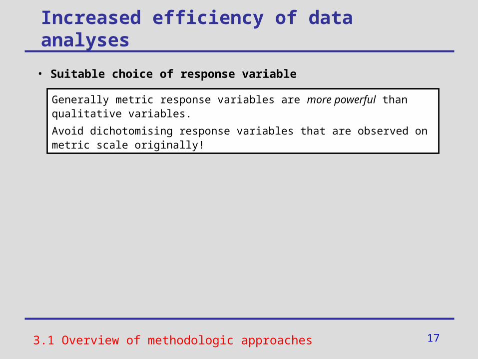
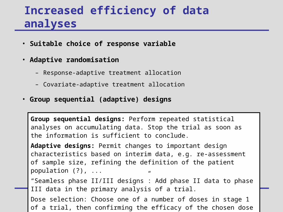
• Suitable choice of response variable
• Adaptive randomisation
– Response-adaptive treatment allocation
– Covariate-adaptive treatment allocation
• Group sequential (adaptive) designs
• Repeated measurement designs (Longitudinal data analysis, incl. N-of-1 designs)
• Adjustment for prognostic variables, Analysis of variances
• Nonparametric resampling methods
• Bayesian methods
3.1 Overview of methodologic approaches
Increased efficiency of data analyses
Generally metric response variables are more powerful than qualitative variables.
Avoid dichotomising response variables that are observed on metric scale originally!
18
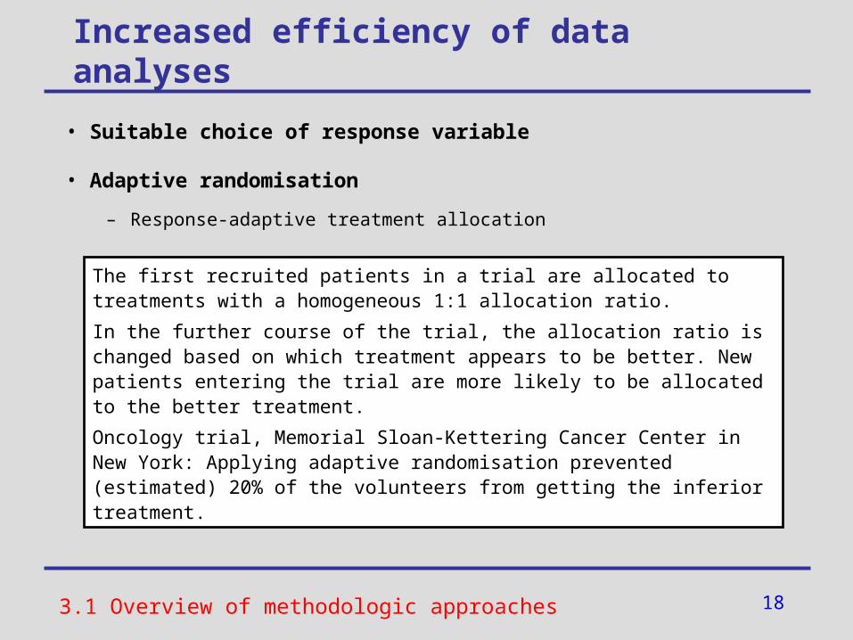
• Suitable choice of response variable
• Adaptive randomisation
– Response-adaptive treatment allocation
– Covariate-adaptive treatment allocation
• Group sequential (adaptive) designs
• Repeated measurement designs (Longitudinal data analysis, incl. N-of-1 designs)
• Adjustment for prognostic variables, Analysis of variances
• Nonparametric resampling methods
• Bayesian methods
3.1 Overview of methodologic approaches
Increased efficiency of data analyses
The first recruited patients in a trial are allocated to treatments with a homogeneous 1:1 allocation ratio.
In the further course of the trial, the allocation ratio is changed based on which treatment appears to be better. New patients entering the trial are more likely to be allocated to the better treatment.
Oncology trial, Memorial Sloan-Kettering Cancer Center in New York: Applying adaptive randomisation prevented (estimated) 20% of the volunteers from getting the inferior treatment.
19
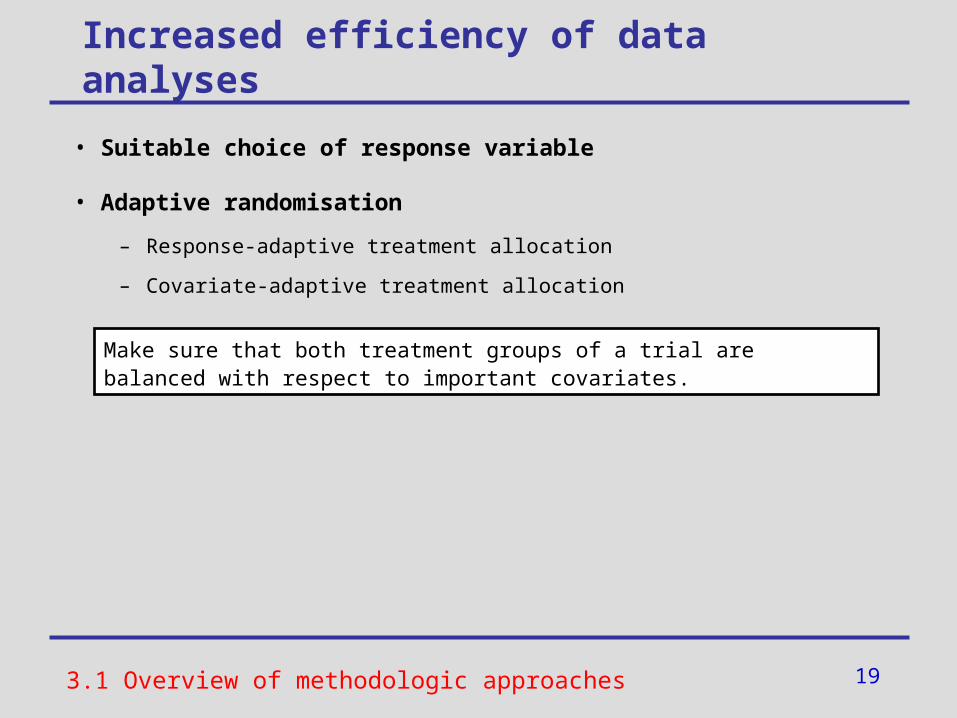
• Suitable choice of response variable
• Adaptive randomisation
– Response-adaptive treatment allocation
– Covariate-adaptive treatment allocation
• Group sequential (adaptive) designs
• Repeated measurement designs (Longitudinal data analysis, incl. N-of-1 designs)
• Adjustment for prognostic variables, Analysis of variances
• Nonparametric resampling methods
• Bayesian methods
3.1 Overview of methodologic approaches
Increased efficiency of data analyses
Make sure that both treatment groups of a trial are balanced with respect to important covariates.
20
• Suitable choice of response variable
• Adaptive randomisation
– Response-adaptive treatment allocation
– Covariate-adaptive treatment allocation
• Group sequential (adaptive) designs
• Repeated measurement designs (Longitudinal data analysis, incl. N-of-1 designs)
• Adjustment for prognostic variables, Analysis of variances
• Nonparametric resampling methods
• Bayesian methods
Increased efficiency of data analyses
Group sequential designs: Perform repeated statistical analyses on accumulating data. Stop the trial as soon as the information is sufficient to conclude.
Adaptive designs: Permit changes to important design characteristics based on interim data, e.g. re-assessment of sample size, refining the definition of the patient population (?), ...
“Seamless phase II/III designs”: Add phase II data to phase III data in the primary analysis of a trial.
Dose selection: Choose one of a number of doses in stage 1 of a trial, then confirming the efficacy of the chosen dose in stage 2.
21
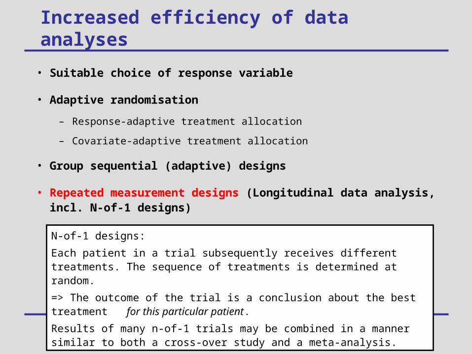
• Suitable choice of response variable
• Adaptive randomisation
– Response-adaptive treatment allocation
– Covariate-adaptive treatment allocation
• Group sequential (adaptive) designs
• Repeated measurement designs (Longitudinal data analysis, incl. N-of-1 designs)
• Adjustment for prognostic variables, Analysis of variances
• Nonparametric resampling methods
• Bayesian methods
Increased efficiency of data analyses
N-of-1 designs:
Each patient in a trial subsequently receives different treatments. The sequence of treatments is determined at random.
=> The outcome of the trial is a conclusion about the best treatment for this particular patient.
Results of many n-of-1 trials may be combined in a manner similar to both a cross-over study and a meta-analysis.
22
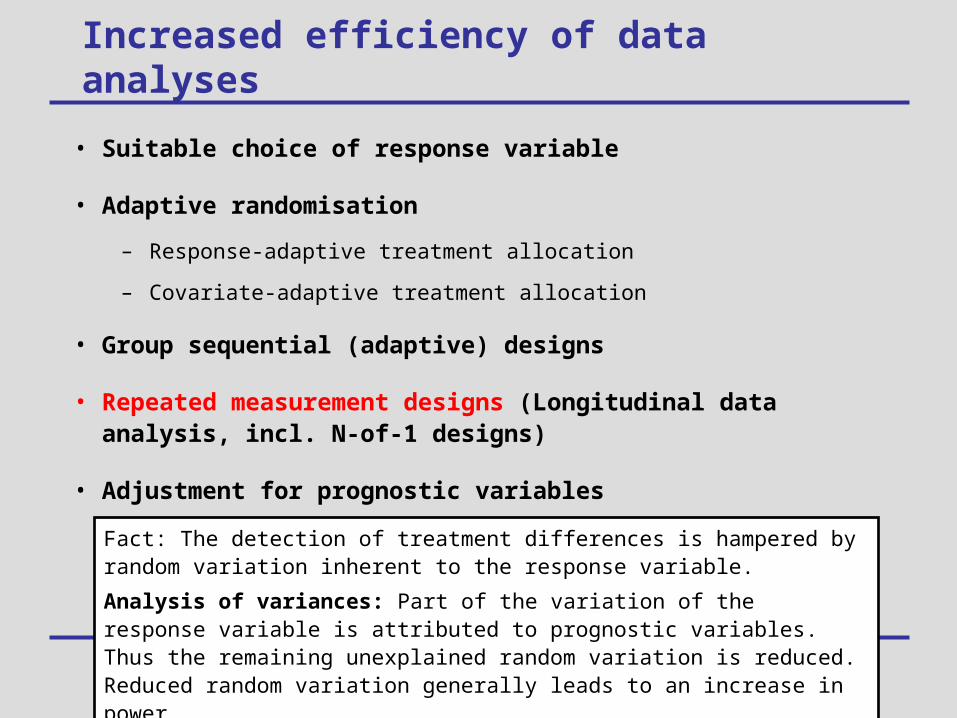
• Suitable choice of response variable
• Adaptive randomisation
– Response-adaptive treatment allocation
– Covariate-adaptive treatment allocation
• Group sequential (adaptive) designs
• Repeated measurement designs (Longitudinal data analysis, incl. N-of-1 designs)
• Adjustment for prognostic variables
• Nonparametric resampling methods
• Bayesian methods
Increased efficiency of data analyses
Fact: The detection of treatment differences is hampered by random variation inherent to the response variable.
Analysis of variances: Part of the variation of the response variable is attributed to prognostic variables. Thus the remaining unexplained random variation is reduced. Reduced random variation generally leads to an increase in power.
23
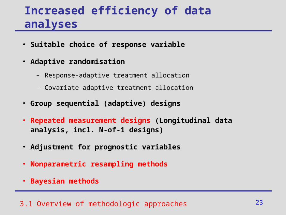
• Suitable choice of response variable
• Adaptive randomisation
– Response-adaptive treatment allocation
– Covariate-adaptive treatment allocation
• Group sequential (adaptive) designs
• Repeated measurement designs (Longitudinal data analysis, incl. N-of-1 designs)
• Adjustment for prognostic variables
• Nonparametric resampling methods
• Bayesian methods
3.1 Overview of methodologic approaches
Increased efficiency of data analyses
24
Outline
1. The innovative drug development approaches-project
2. Weakness of small sample trials
3. Increase the efficiency of statistical data analyses
3.1 Overview of methodologic approaches
3.2 Resampling
3.3 Repeated measurement designs
3.4 Bayesian models
4. Software
5. Summary and Conclusion
25
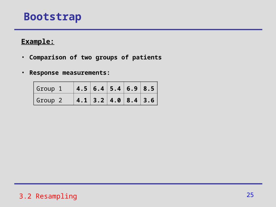
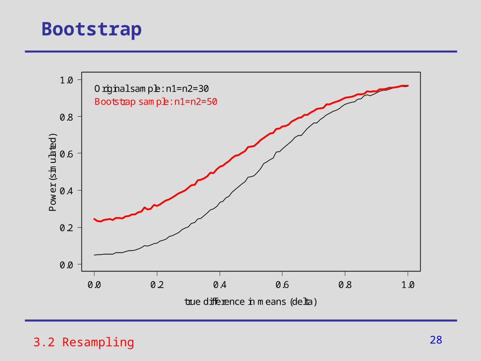
Bootstrap
Example:
• Comparison of two groups of patients
• Response measurements:
3.2 Resampling
Group 1 4.5 6.4 5.4 6.9 8.5
Group 2 4.1 3.2 4.0 8.4 3.6
26
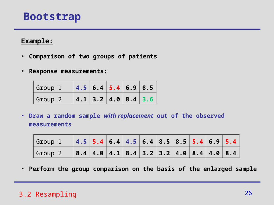
Bootstrap
Example:
• Comparison of two groups of patients
• Response measurements:
• Draw a random sample with replacement out of the observed measurements
• Perform the group comparison on the basis of the enlarged sample
3.2 Resampling
Group 1 4.5 6.4 5.4 6.9 8.5
Group 2 4.1 3.2 4.0 8.4 3.6
Group 1 4.5 5.4 6.4 4.5 6.4 8.5 8.5 5.4 6.9 5.4
Group 2 8.4 4.0 4.1 8.4 3.2 3.2 4.0 8.4 4.0 8.4
27
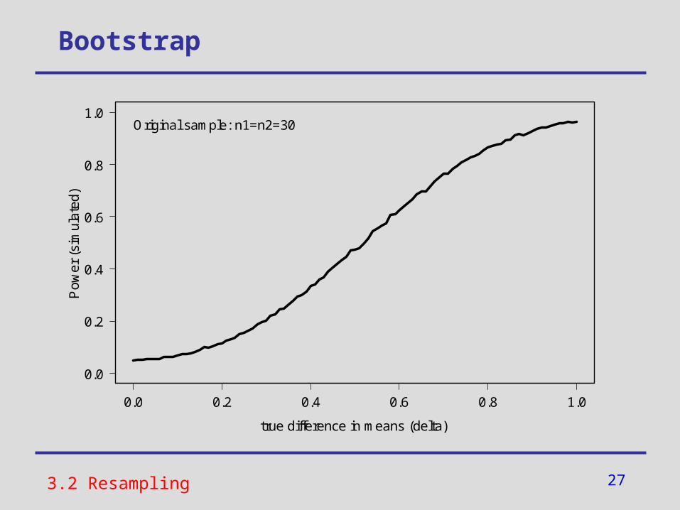
Bootstrap
3.2 Resampling
0.0 0.2 0.4 0.6 0.8 1.0
0.0
0.2
0.4
0.6
0.8
1.0
true difference in means (delta)
Pow
er (
sim
ulat
ed)
Original sample: n1=n2=30
28
Bootstrap
3.2 Resampling
0.0 0.2 0.4 0.6 0.8 1.0
0.0
0.2
0.4
0.6
0.8
1.0
true difference in means (delta)
Pow
er (
sim
ulat
ed)
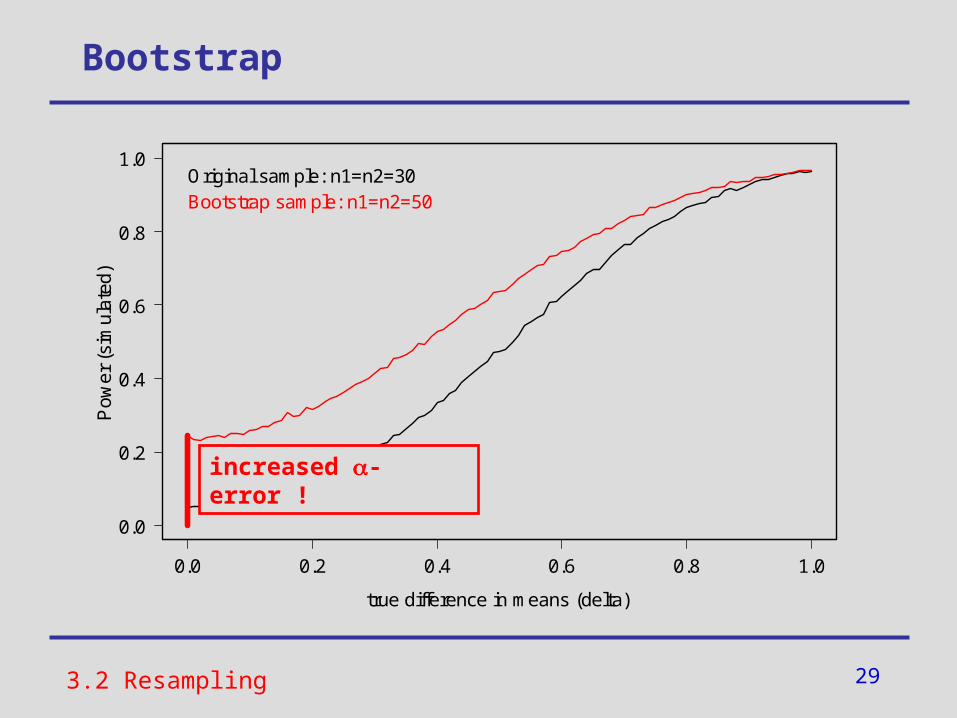
Original sample: n1=n2=30Bootstrap sample: n1=n2=50
29
Bootstrap
3.2 Resampling
0.0 0.2 0.4 0.6 0.8 1.0
0.0
0.2
0.4
0.6
0.8
1.0
true difference in means (delta)
Pow
er (
sim
ulat
ed)
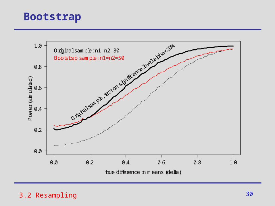
Original sample: n1=n2=30Bootstrap sample: n1=n2=50
increased -error !
30
Bootstrap
3.2 Resampling
0.0 0.2 0.4 0.6 0.8 1.0
0.0
0.2
0.4
0.6
0.8
1.0
true difference in means (delta)
Pow
er (
sim
ulat
ed)
Original sample: n1=n2=30Bootstrap sample: n1=n2=50
Original s
ample, test o
n significance
leve
l alpha=20%
31
Outline
1. The innovative drug development approaches-project
2. Weakness of small sample trials
3. Increase the efficiency of statistical data analyses
3.1 Overview of methodologic approaches
3.2 Resampling
3.3 Repeated measurement designs
3.4 Bayesian models
4. Software
5. Summary and Conclusion
32
Example 1: Binary response variable
• Clinical trial with two parallel treatment groups and binary response variable
• Two different possible designs:
(a) (b)
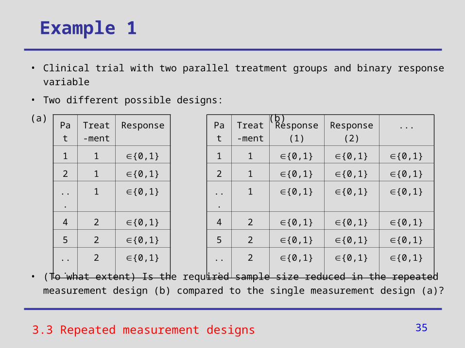
• (To what extent) Is the required sample size reduced in the repeated measurement design (b) compared to the single measurement design (a)?
3.3 Repeated measurement designs
33
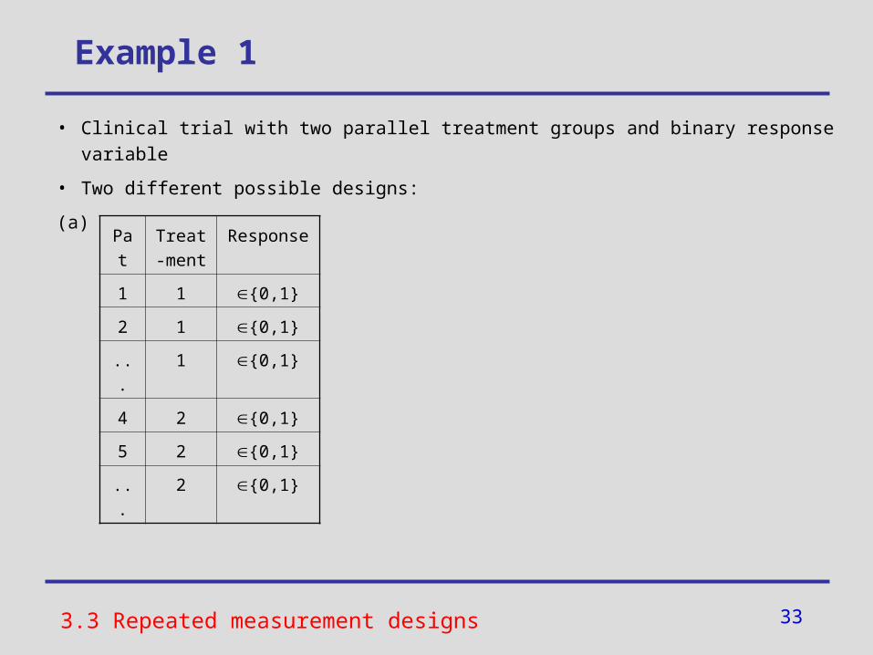
Example 1
• Clinical trial with two parallel treatment groups and binary response variable
• Two different possible designs:
(a) (b)
• (To what extent) Is the required sample size reduced in the repeated measurement design (b) compared to the single measurement design (a)?
3.3 Repeated measurement designs
Pat Treat-ment
Response
1 1 {0,1}
2 1 {0,1}
... 1 {0,1}
4 2 {0,1}
5 2 {0,1}
... 2 {0,1}
34
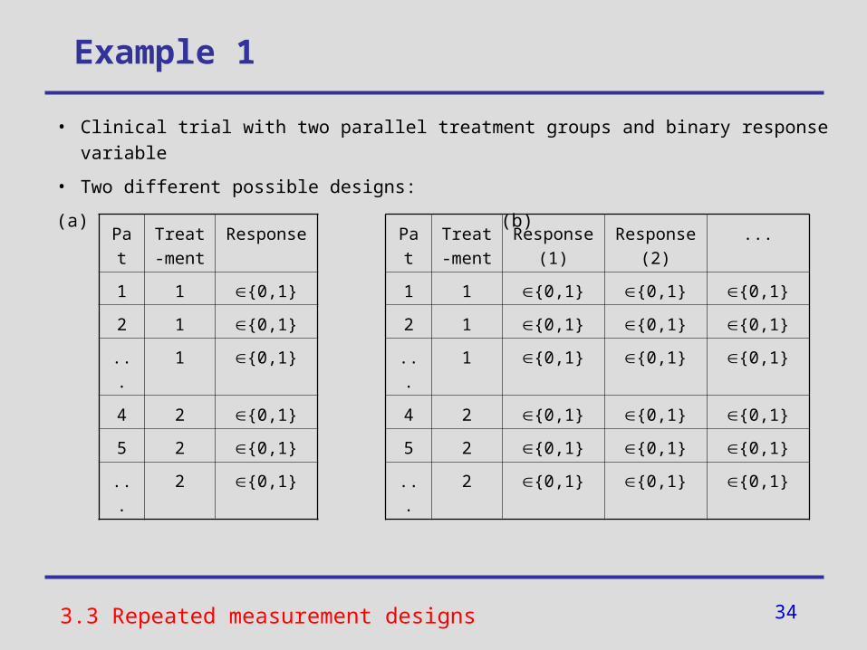
Example 1
• Clinical trial with two parallel treatment groups and binary response variable
• Two different possible designs:
(a) (b)
• (To what extent) Is the required sample size reduced in the repeated measurement design (b) compared to the single measurement design (a)?
3.3 Repeated measurement designs
Pat Treat-ment
Response
1 1 {0,1}
2 1 {0,1}
... 1 {0,1}
4 2 {0,1}
5 2 {0,1}
... 2 {0,1}
Pat Treat-ment
Response (1)
Response (2)
...
1 1 {0,1} {0,1} {0,1}
2 1 {0,1} {0,1} {0,1}
... 1 {0,1} {0,1} {0,1}
4 2 {0,1} {0,1} {0,1}
5 2 {0,1} {0,1} {0,1}
... 2 {0,1} {0,1} {0,1}
35
Example 1
• Clinical trial with two parallel treatment groups and binary response variable
• Two different possible designs:
(a) (b)
• (To what extent) Is the required sample size reduced in the repeated measurement design (b) compared to the single measurement design (a)?
3.3 Repeated measurement designs
Pat Treat-ment
Response
1 1 {0,1}
2 1 {0,1}
... 1 {0,1}
4 2 {0,1}
5 2 {0,1}
... 2 {0,1}
Pat Treat-ment
Response (1)
Response (2)
...
1 1 {0,1} {0,1} {0,1}
2 1 {0,1} {0,1} {0,1}
... 1 {0,1} {0,1} {0,1}
4 2 {0,1} {0,1} {0,1}
5 2 {0,1} {0,1} {0,1}
... 2 {0,1} {0,1} {0,1}
36
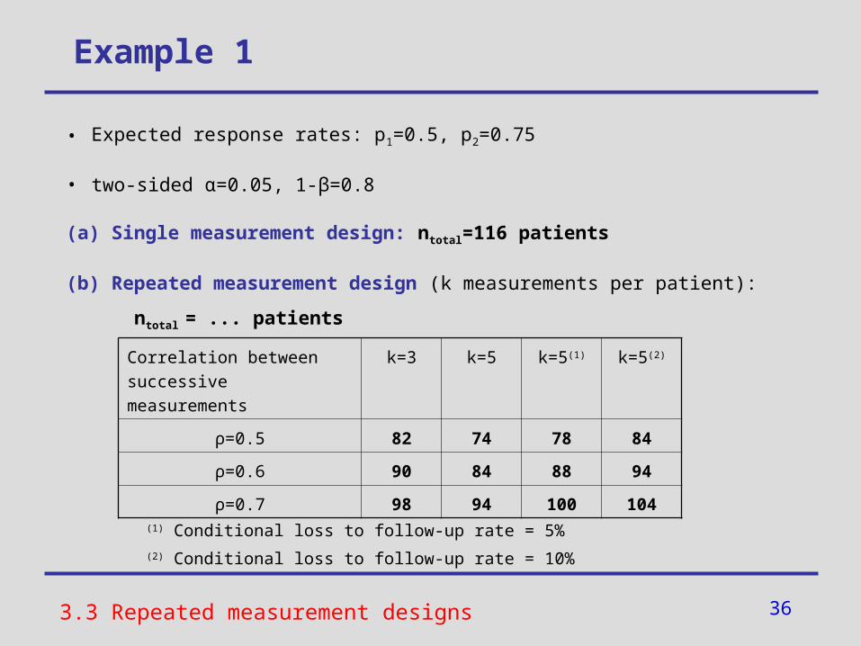
• Expected response rates: p1=0.5, p2=0.75
• two-sided α=0.05, 1-β=0.8
(a) Single measurement design: ntotal=116 patients
(b) Repeated measurement design (k measurements per patient):
ntotal = ... patients
(1) Conditional loss to follow-up rate = 5% (2) Conditional loss to follow-up rate = 10%
3.3 Repeated measurement designs
Correlation between successive measurements
k=3 k=5 k=5(1) k=5(2)
ρ=0.5 82 74 78 84
ρ=0.6 90 84 88 94
ρ=0.7 98 94 100 104
Example 1
37
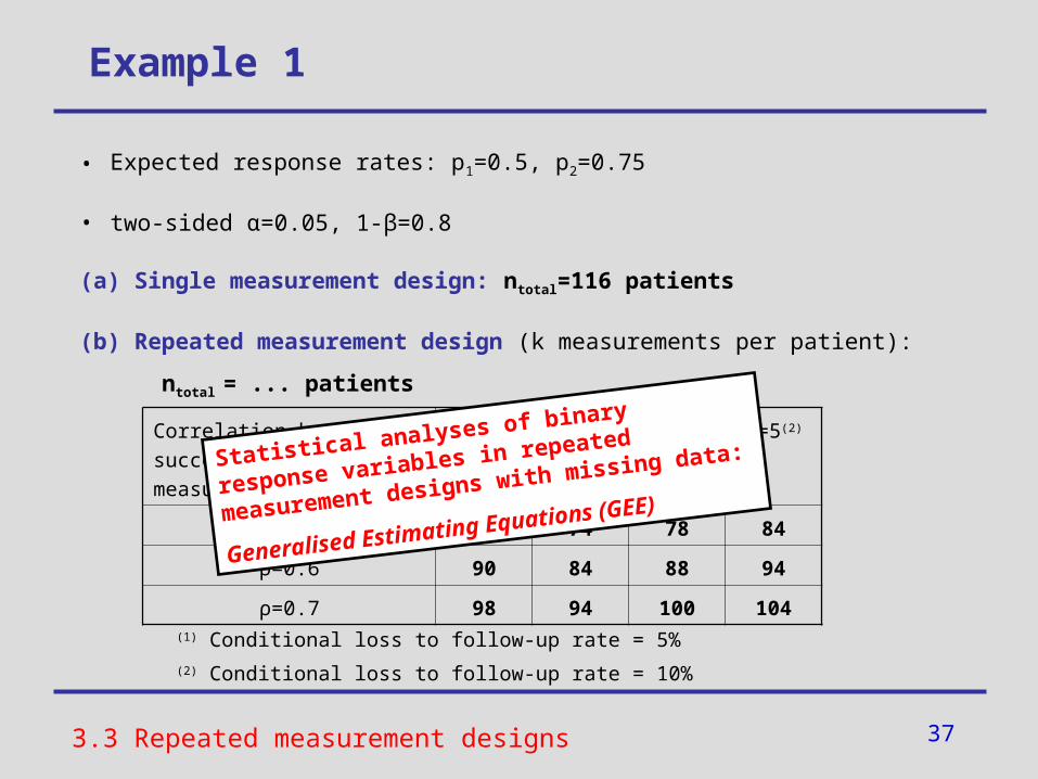
• Expected response rates: p1=0.5, p2=0.75
• two-sided α=0.05, 1-β=0.8
(a) Single measurement design: ntotal=116 patients
(b) Repeated measurement design (k measurements per patient):
ntotal = ... patients
(1) Conditional loss to follow-up rate = 5% (2) Conditional loss to follow-up rate = 10%
3.3 Repeated measurement designs
Correlation between successive measurements
k=3 k=5 k=5(1) k=5(2)
ρ=0.5 82 74 78 84
ρ=0.6 90 84 88 94
ρ=0.7 98 94 100 104
Example 1
Statistical analyses of binary response
variables in repeated measurement
designs with missing data:
Generalised Estimating Equations (GEE)
38
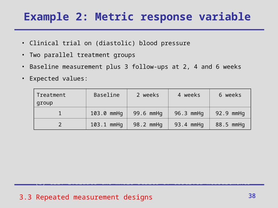
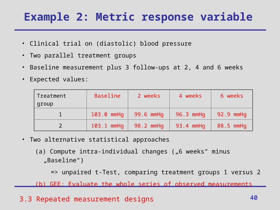
Example 2: Metric response variable
• Clinical trial on (diastolic) blood pressure
• Two parallel treatment groups
• Baseline measurement plus 3 follow-ups at 2, 4 and 6 weeks
• Expected values:
• Two alternative statistical approaches
(a) Compute intra-individual changes („6 weeks“ minus „Baseline“)
=> unpaired t-Test, comparing treatment groups 1 versus 2
(b) GEE: Evaluate the whole series of observed measurements
3.3 Repeated measurement designs
Treatment group Baseline 2 weeks 4 weeks 6 weeks
1 103.0 mmHg 99.6 mmHg 96.3 mmHg 92.9 mmHg
2 103.1 mmHg 98.2 mmHg 93.4 mmHg 88.5 mmHg
39
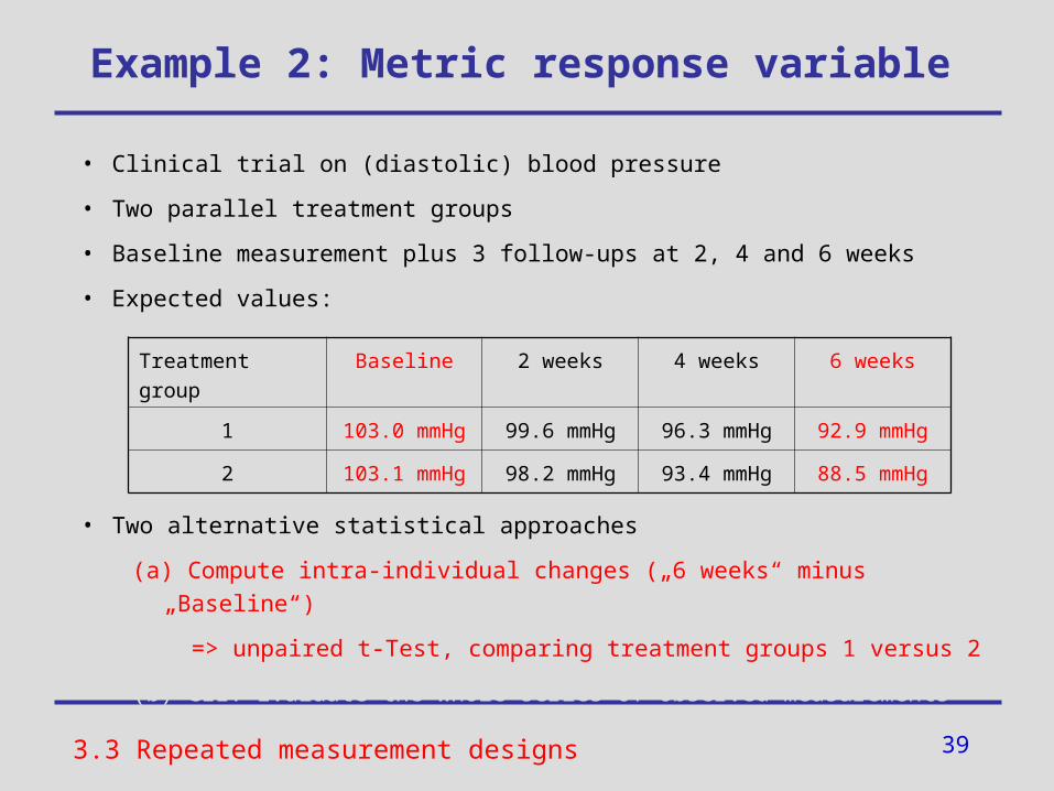
Example 2: Metric response variable
• Clinical trial on (diastolic) blood pressure
• Two parallel treatment groups
• Baseline measurement plus 3 follow-ups at 2, 4 and 6 weeks
• Expected values:
• Two alternative statistical approaches
(a) Compute intra-individual changes („6 weeks“ minus „Baseline“)
=> unpaired t-Test, comparing treatment groups 1 versus 2
(b) GEE: Evaluate the whole series of observed measurements
3.3 Repeated measurement designs
Treatment group Baseline 2 weeks 4 weeks 6 weeks
1 103.0 mmHg 99.6 mmHg 96.3 mmHg 92.9 mmHg
2 103.1 mmHg 98.2 mmHg 93.4 mmHg 88.5 mmHg
40
Example 2: Metric response variable
• Clinical trial on (diastolic) blood pressure
• Two parallel treatment groups
• Baseline measurement plus 3 follow-ups at 2, 4 and 6 weeks
• Expected values:
• Two alternative statistical approaches
(a) Compute intra-individual changes („6 weeks“ minus „Baseline“)
=> unpaired t-Test, comparing treatment groups 1 versus 2
(b) GEE: Evaluate the whole series of observed measurements
3.3 Repeated measurement designs
Treatment group Baseline 2 weeks 4 weeks 6 weeks
1 103.0 mmHg 99.6 mmHg 96.3 mmHg 92.9 mmHg
2 103.1 mmHg 98.2 mmHg 93.4 mmHg 88.5 mmHg
41
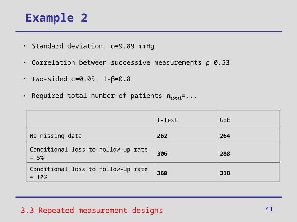
Example 2
• Standard deviation: σ=9.89 mmHg
• Correlation between successive measurements ρ=0.53
• two-sided α=0.05, 1-β=0.8
• Required total number of patients ntotal=...
3.3 Repeated measurement designs
t-Test GEE
No missing data 262 264
Conditional loss to follow-up rate = 5% 306 288
Conditional loss to follow-up rate = 10% 360 318
42
Outline
1. The innovative drug development approaches-project
2. Weakness of small sample trials
3. Increase the efficiency of statistical data analyses
3.1 Overview of methodologic approaches
3.2 Resampling
3.3 Repeated measurement designs
3.4 Bayesian models
4. Software
5. Summary and Conclusion
43
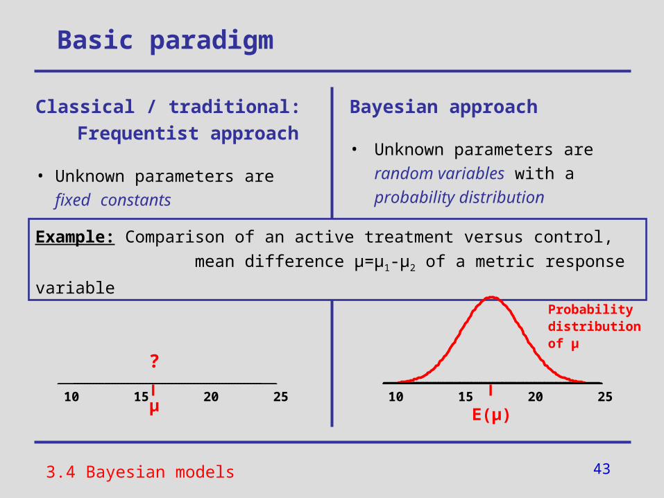
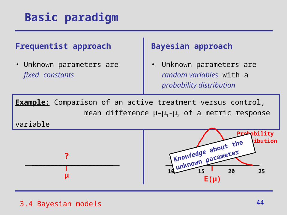
Classical / traditional: Frequentist approach
• Unknown parameters are fixed constants
Basic paradigm
3.4 Bayesian models
Bayesian approach
• Unknown parameters are random variables with a probability distribution
Example: Comparison of an active treatment versus control,
mean difference µ=µ1-µ2 of a metric response variable
10 15 20 25
Probability distribution of µ
E(µ)
―
µ
―
?
10 15 20 25
44
Frequentist approach
• Unknown parameters are fixed constants
Basic paradigm
3.4 Bayesian models
Bayesian approach
• Unknown parameters are random variables with a probability distribution
Example: Comparison of an active treatment versus control,
mean difference µ=µ1-µ2 of a metric response variable
10 15 20 25
Probability distribution of µ
E(µ)
―
µ
―
? Knowledge about the
unknown parameter
45
Prior and posterior distribution
Example: Mean difference of a metric response variable µ=µ1-µ2
-> „To what extent is the active treatment superior to control?“
• Model the knowledge about the unknown parameter:
1. Before collecting data of the present trial „prior distribution p(µ)“
2. Collect new data and combine the prior knowledge with the information provided by newly collected data => posterior distribution p(µ|data)
• Inference is carried out on the basis of the posterior distribution of the parameter of interest.
• Bayesian data analyses are based upon a completely different paradigm compared to frequentist methods (e.g. there exist no „Bayesian p-values“).
3.4 Bayesian models
46
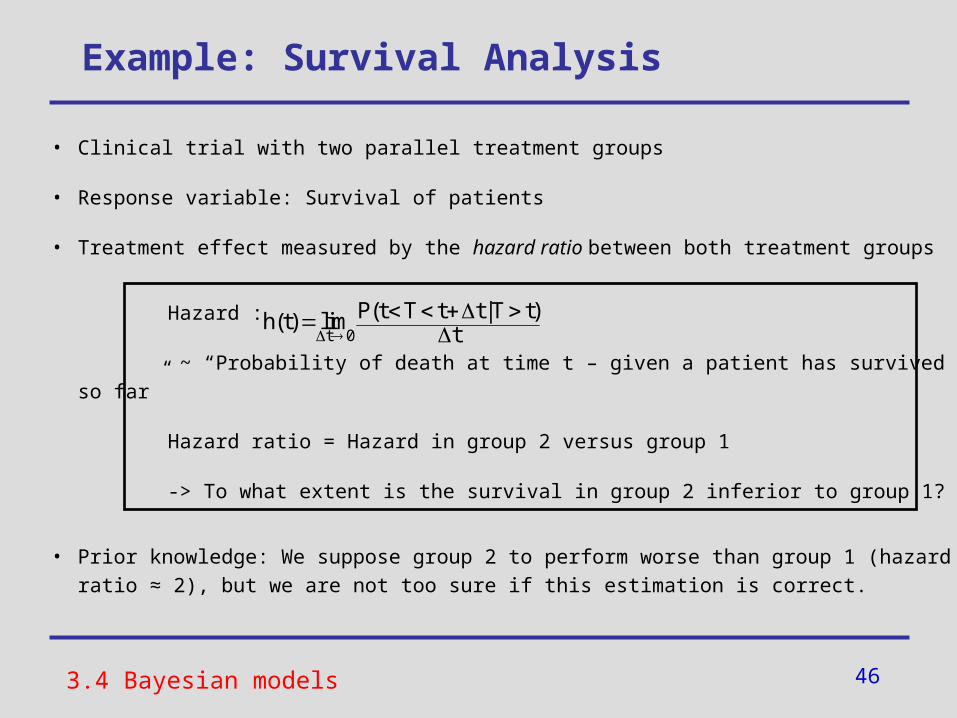
Example: Survival Analysis
• Clinical trial with two parallel treatment groups
• Response variable: Survival of patients
• Treatment effect measured by the hazard ratio between both treatment groups
Hazard :
~ “Probability of death at time t – given a patient has survived so far”
Hazard ratio = Hazard in group 2 versus group 1
-> To what extent is the survival in group 2 inferior to group 1?
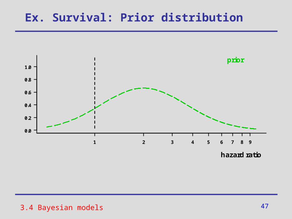
• Prior knowledge: We suppose group 2 to perform worse than group 1 (hazard ratio ≈ 2), but we are not too sure if this estimation is correct.
3.4 Bayesian models
t 0
P(t T t t |T t)h(t) limt
47
Ex. Survival: Prior distribution
3.4 Bayesian models
1 2 3 4 5 6 7 8 9
0.0
0.2
0.4
0.6
0.8
1.0
hazard ratio
prior
48
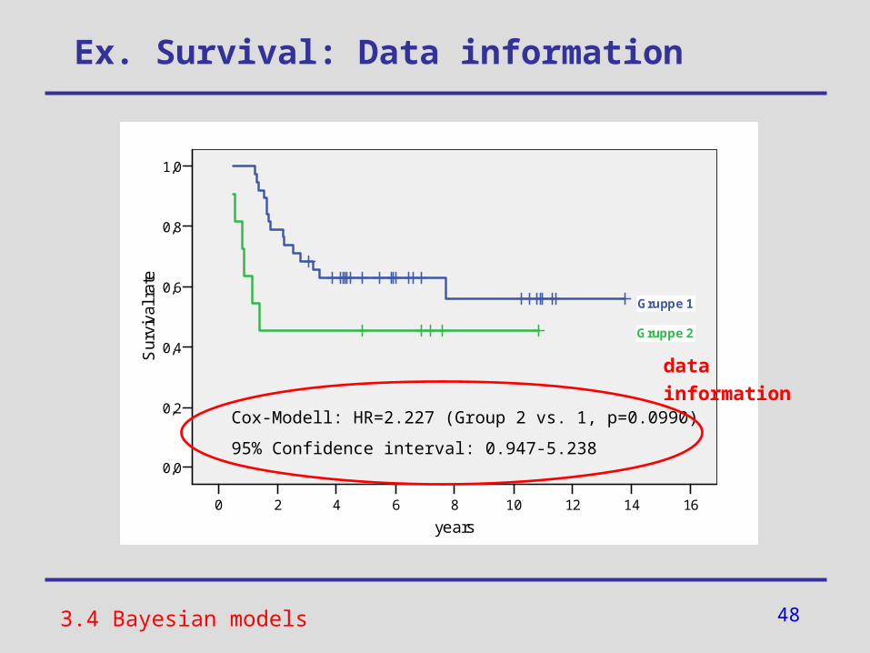
Ex. Survival: Data information
3.4 Bayesian models
1614121086420
years
1,0
0,8
0,6
0,4
0,2
0,0
Sur
viva
l rat
e
Gruppe 2
Gruppe 1
Cox-Modell: HR=2.227 (Group 2 vs. 1, p=0.0990)
95% Confidence interval: 0.947-5.238
data information
49
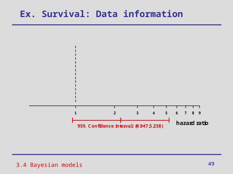
Ex. Survival: Data information
3.4 Bayesian models
1 2 3 4 5 6 7 8 9
95% Confidence interval: (0.947,5.238)hazard ratio
50
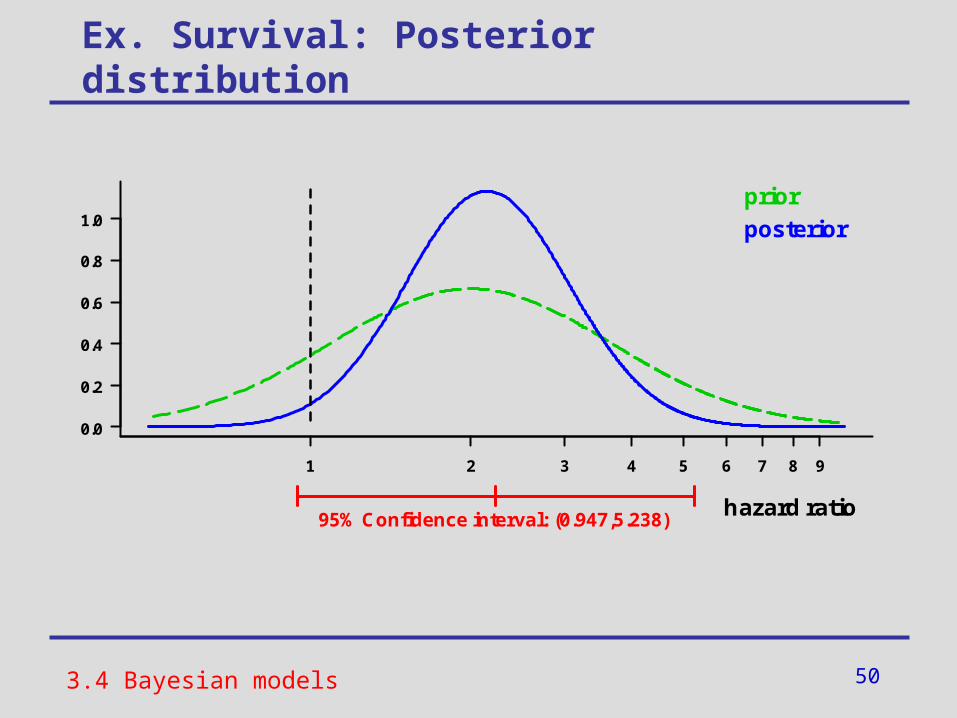
Ex. Survival: Posterior distribution
3.4 Bayesian models
1 2 3 4 5 6 7 8 9
0.0
0.2
0.4
0.6
0.8
1.0
95% Confidence interval: (0.947,5.238)hazard ratio
prior
posterior
51
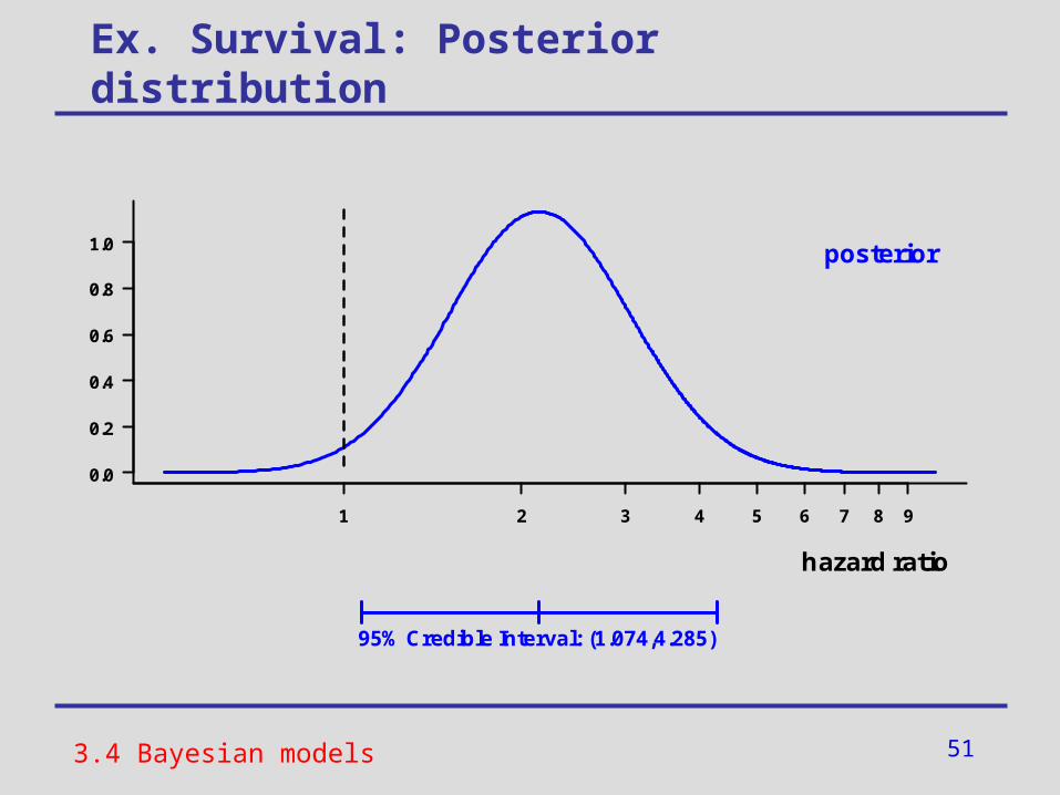
Ex. Survival: Posterior distribution
3.4 Bayesian models
1 2 3 4 5 6 7 8 9
0.0
0.2
0.4
0.6
0.8
1.0
hazard ratio
posterior
95% Credible Interval: (1.074,4.285)
52
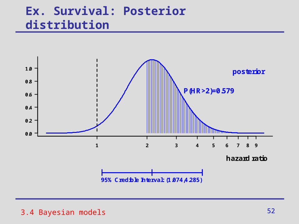
Ex. Survival: Posterior distribution
3.4 Bayesian models
1 2 3 4 5 6 7 8 9
0.0
0.2
0.4
0.6
0.8
1.0
hazard ratio
posterior
95% Credible Interval: (1.074,4.285)
P(HR>2)=0.579
53
Ex. Survival: Prior and posterior distn
3.4 Bayesian models
1 2 3 4 5 6 7 8 9
0.0
0.5
1.0
1.5
2.0
95% Confidence interval: (0.947,5.238)hazard ratio
prior
posterior
95% Credible Interval: (2.53,5.16)
54
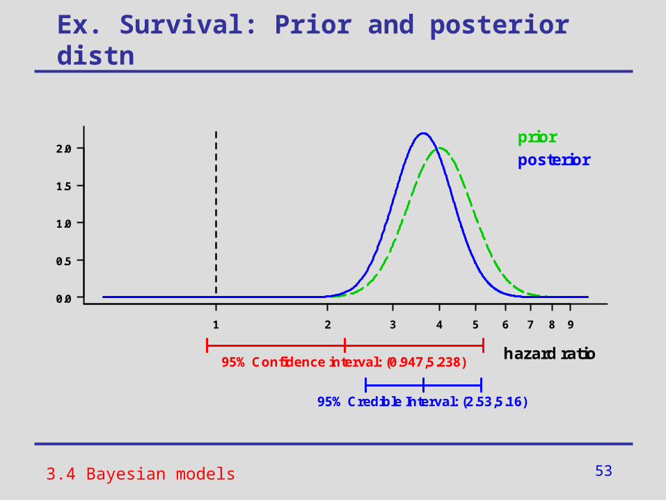
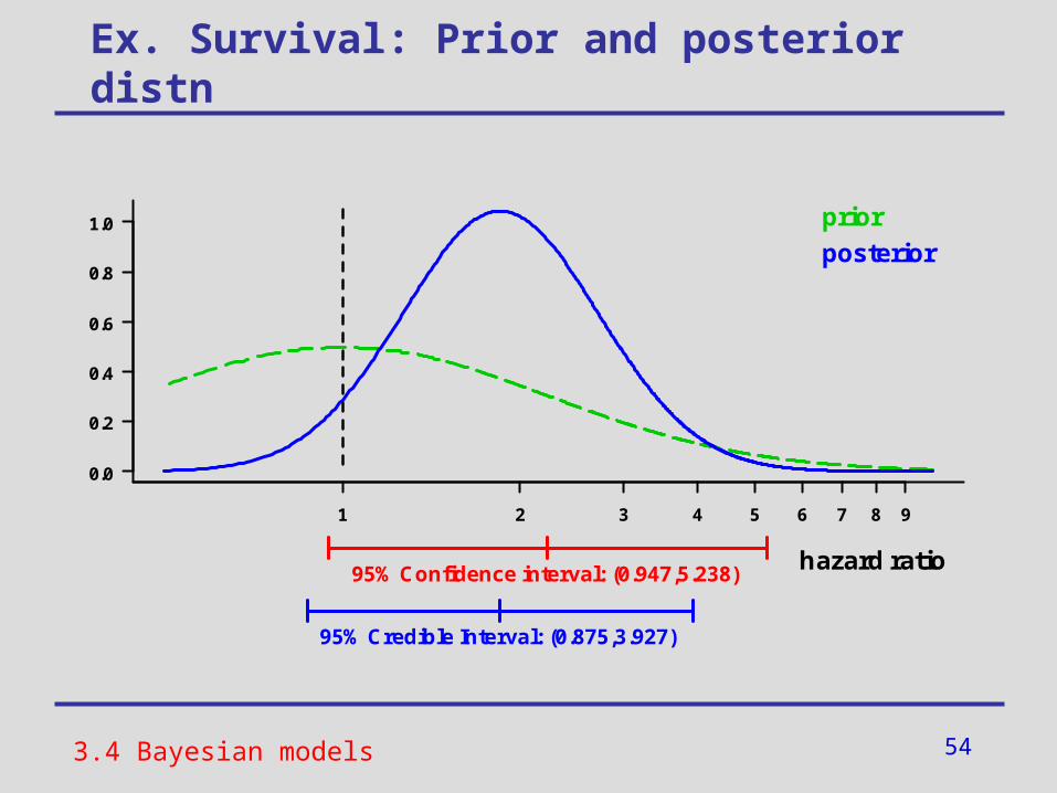
Ex. Survival: Prior and posterior distn
3.4 Bayesian models
1 2 3 4 5 6 7 8 9
0.0
0.2
0.4
0.6
0.8
1.0
95% Confidence interval: (0.947,5.238)hazard ratio
prior
posterior
95% Credible Interval: (0.875,3.927)
55
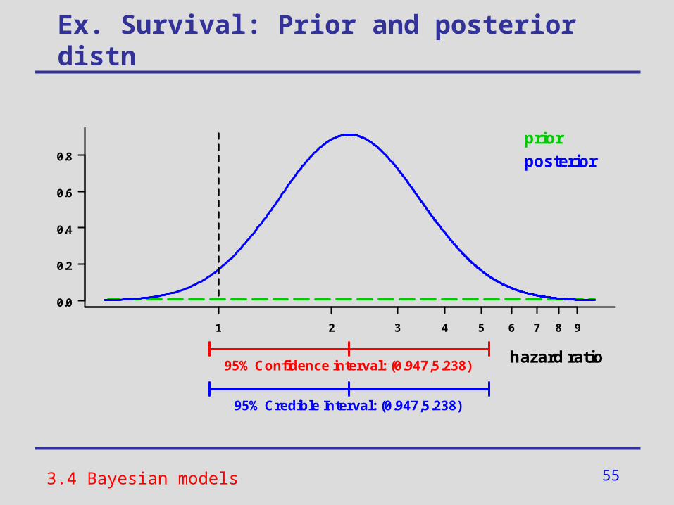
Ex. Survival: Prior and posterior distn
3.4 Bayesian models
1 2 3 4 5 6 7 8 9
0.0
0.2
0.4
0.6
0.8
95% Confidence interval: (0.947,5.238)hazard ratio
prior
posterior
95% Credible Interval: (0.947,5.238)
56
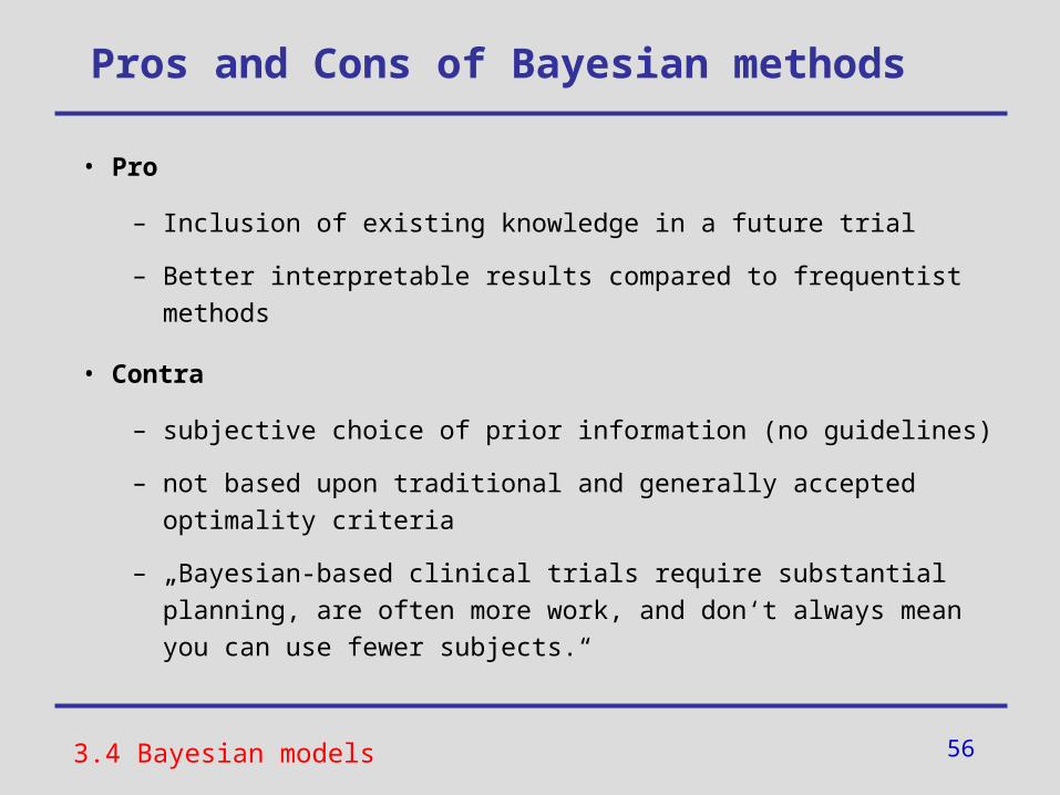
Pros and Cons of Bayesian methods
• Pro
– Inclusion of existing knowledge in a future trial
– Better interpretable results compared to frequentist methods
• Contra
– subjective choice of prior information (no guidelines)
– not based upon traditional and generally accepted optimality criteria
– „Bayesian-based clinical trials require substantial planning, are often more work, and don‘t always mean you can use fewer subjects.“
3.4 Bayesian models
57
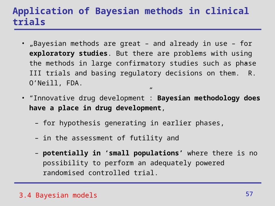
Application of Bayesian methods in clinical trials
• „Bayesian methods are great – and already in use – for exploratory studies. But there are problems with using the methods in large confirmatory studies such as phase III trials and basing regulatory decisions on them.” R. O’Neill, FDA.
• “Innovative drug development”: Bayesian methodology does have a place in drug development,
– for hypothesis generating in earlier phases,
– in the assessment of futility and
– potentially in ‘small populations’ where there is no possibility to perform an adequately powered randomised controlled trial.
3.4 Bayesian models
58
Outline
1. The innovative drug development approaches-project
2. Weakness of small sample trials
3. Increase the efficiency of statistical data analyses
3.1 Overview of methodologic approaches
3.2 Resampling
3.3 Repeated measurement designs
3.4 Bayesian models
4. Software
5. Summary and Conclusion
59
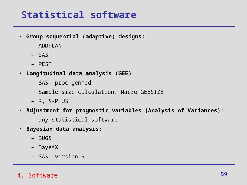
Statistical software
• Group sequential (adaptive) designs:
– ADDPLAN
– EAST
– PEST
• Longitudinal data analysis (GEE)
– SAS, proc genmod
– Sample-size calculation: Macro GEESIZE
– R, S-PLUS
• Adjustment for prognostic variables (Analysis of Variances):
– any statistical software
• Bayesian data analysis:
– BUGS
– BayesX
– SAS, version 9
4. Software
60
Outline
1. The innovative drug development approaches-project
2. Weakness of small sample trials
3. Increase the efficiency of statistical data analyses
3.1 Overview of methodologic approaches
3.2 Resampling
3.3 Repeated measurement designs
3.4 Bayesian models
4. Software
5. Summary and Conclusion
61
Summary and Conclusion
• There are methodological approaches that can be applied to increase the efficiency of the statistical analysis in small sample trials.
• Each single approach itself yields only a small increase in efficiency indeed. But combining the different approaches, a substantial increase in efficiency may be obtained.
• The possibilities however are not unlimited naturally. In case of a too small sample size, one has to compensate for this by „paying a price“. This price may be
– required additional (possibly restrictive) model assumptions.
– defeasibility and reduced acceptance of the results obtained.
• Bayesian methods represent a promising alternative to classical frequentist analyses and their application is accepted in exploratory problems. In confirmatory problems, Bayesian methods may be maintainable only in special situations (e.g. small sample trials). Otherwise a paradigm shift towards Bayesian methods is not accepted by regulatory authorities.
5. Summary and Conclusion
62
Literature
• EMEA Publications
– Innovative Drug Development Approaches (March 2007)
– Guideline on Clinical Trials in Small Populations (July 2006)
• Generalised Estimating Equations (GEE)
– Dahmen, Rochon, König, Ziegler (2004): Sample Size Calculations for Controlled Clinical Trials Using Generalized Estimating Equations (GEE). Methods Inf Med 43: 451-6.
– Dahmen, Ziegler (2006): Independence Estimating Equations for Controlled Clinical Trials with Small Sample Sizes. Methods Inf Med 45: 430-4.
– Liang, Zeger (1986): Longitudinal Data Analysis Using Generalized Linear Models. Biometrika 73, 13 - 22.
• Bayesian data analysis
– Spiegelhalter, Abrams, Myles (2004): Bayesian Approaches to Clinical Trials and Health-Care Evaluation, Wiley.
Thank you for your attention!