Embed Size (px)
Citation preview
General rights Copyright and moral rights for the publications made accessible in the public portal are retained by the authors and/or other copyright owners and it is a condition of accessing publications that users recognise and abide by the legal requirements associated with these rights.
Users may download and print one copy of any publication from the public portal for the purpose of private study or research.
You may not further distribute the material or use it for any profit-making activity or commercial gain
You may freely distribute the URL identifying the publication in the public portal If you believe that this document breaches copyright please contact us providing details, and we will remove access to the work immediately and investigate your claim.
Downloaded from orbit.dtu.dk on: Feb 18, 2019
Icing Problems of Wind Turbine Blades in Cold Climates
Hudecz, Adriána; Hansen, Martin Otto Laver; Battisti, Lorenzo; Villumsen, Arne
Publication date:2014
Document VersionPublisher's PDF, also known as Version of record
Link back to DTU Orbit
Citation (APA):Hudecz, A., Hansen, M. O. L., Battisti, L., & Villumsen, A. (2014). Icing Problems of Wind Turbine Blades in ColdClimates. Department of Wind Energy, Technical University of Denmark.
IC
A
D
N
DTU
Vin
dene
rgi
PhD
Rap
port
2013
cing PClima
Adriána Hude
DTU Wind En
November 20
PhD
Rap
port
2013
Problates
ecz
nergy PhD-00
013
ems o
031 (EN)
of Wind Tuurbinee Bladdes inn Coldd

Forfatter(e): Adriána Hudecz
Titel: Icing Problems of Wind Turbine Blades in Cold Climates
Department: DTU Wind Energy
DTU Wind Energy PhD-0031 (EN)
November 2013
ISBN: 978-87-92896-80-3
Resumen (maks 2000 char.):
Due to the ambitious targets on increasing the use of renewable energy
sources and also the lack of conventional sites, non-conventional sites, e.g.
cold climate (CC) sites are getting more attractive to wind turbine
installations. Deployment of wind energy in CC areas grows rapidly. The
installed wind power capacity at the end of 2012 was around 69GW, which
corresponds to approximately 24% of the total (globally) installed capacity.
Operation of wind turbines is challenging at CC sites. Wind turbines at these
sites may be exposed to icing conditions or temperatures outside the design
limits of standard wind turbines. Cold climate plays a major role in power
production and safety hazards of a wind turbine. Icing is a key parameter in
project development for cold climate operation. These conditions can be
found in sub-arctic or arctic regions, like in the Nordic countries in Europe, in
Canada and at high altitude mountains (e.g. Alps). During the PhD work, the risk of icing events and the effect of ice accretion on wind turbine blades were studied. A small demonstration of how to identify icing event was performed using meteorological data collected in Nanortalik, in South-Greenland. A larger part of the PhD work contains experimental and numerical investigations of the impacts of ice accretion on an airfoil section with different angles of attack. The experimental study was carried out in the Collaborative Climatic Wind Tunnel located at FORCE Technology to investigate how ice accumulates for moderate low temperatures on the blade and how the aerodynamic forces are changing during the process of ice build-up. In the first part of the numerical analysis, the resulted ice profiles of the wind tunnel tests were compared to profiles simulated with using the 2-D ice accretion code whereas in the second part, computational fluid dynamics was used to numerically analyze the impacts of ice accretion on the flow behavior and the aerodynamic characteristics of the airfoil. The PhD study delivered new insights into the research in the field of wind energy in cold climate and gave suggestions for further investigations and improvements.
Projektperiode: 2010.11.15-2013.11.14.
Uddannelse:
Master of Science
Område:
Wind Energy
Vejledere:
Martin Otto Laver Hansen
Lorenzo Battisti
Arne Villumsen
Kontakt.:
Projektnr.:
Sider: 123
Figurer: 80
Tabeller: 20
Referencer: 65
Danmarks Tekniske Universitet Institut for Vindenergi Nils Koppels Allé Bygning 403 2800 Kgs. Lyngby Phone 45254340 [email protected]
www.vindenergi.dtu.dk
Technical University of Denmark
Doctoral Thesis
Icing Problems of Wind Turbine Bladesin Cold Climates
Author:Adriana Hudecz
Supervisor:Martin Otto Laver Hansen
Co-Supervisors:Lorenzo Battisti & Arne Villumsen
A thesis submitted in fulfilment of the requirementsfor the degree of Doctor of Philosophy in engineering
in the
Fluid Mechanics SectionDepartment of Wind Energy
November 18, 2013

ii
Preface
This thesis was prepared at the Department of Wind Energy, Technical University ofDenmark during the period from 15th of November 2010 to 14th of November 2013 inpartial fulfilment of the requirements for acquiring the degree of doctor of philosophy inengineering. The PhD study was carried out under the supervision of associate professorMartin O. L. Hansen and was co-supervised by associate professor Lorenzo Battisti fromTrento University, Italy and professor Arne Villumsen former head of section of ArcticTechnology Center, Technical University of Denmark.
The overall objective of the conducted research was to study the impacts of ice accre-tion on wind turbine blades through experimental and numerical work along with theenvironmental conditions, which are favourable for ice formation on structures. Some ofthe work presented in this thesis was previously disseminated in the following papers andconferences (a copy of the first three journal/conference papers can be found in AppendixE):
� Hudecz, A., Hansen, M. O. L., Dillingh, J. and Turkia, V. (2013). NumericalInvestigation of the Effects of Ice Accretion on a Wind Turbine Blade. Wind Energy.(Submitted)
� Hudecz, A., Koss, H. H. and Hansen, M. O. L. (2013). Icing Wind Tunnel Tests ofa Wind Turbine Blade. Wind Energy. (Submitted)
� Hudecz, A., Koss, H. H. and Hansen, M. O. L. (2013). Ice Accretion on Wind Tur-bine Blades. In XV. International Workshop on Atmospheric Icing on Structures,St-Johns, Newfoundland, September 8 to 11, 2013. (Oral presentation)
� Hudecz, A., Hansen, M. O. L. (2013). Experimental Investigation of Ice Accretion onWind Turbine Blades. In WinterWind 2013, International Wind Energy Conference,12-13. February 2013, Ostersund, Sweden (Electronic poster presentation)
� Hudecz, A., Hansen, M. O. L., Koss, H. H. (2012). Wind Tunnel Tests on Ice Ac-cretion on Wind Turbine Blades. In WinterWind 2012, International Wind EnergyConference, 7-8. February 2012, Skelleftea, Sweden (Electronic poster presentation)
These papers and posters together describe the core of the work. The dissertation com-prises an overall introduction explaining the most fundamental issues and findings of windenergy in cold climates along with three research topics detailed in three separate chap-ters. Each chapter can be considered as an individual unit, however they cohere in somelevel. Each of them starts with a detailed introduction to the specific field and a thoroughliterature study of the recent findings. Some of the results of Chapter 3 and 4 are usedin a demonstration of the transformation method presented by Seifert and Richert [1997]in Chapter 5.

iv
Abstract
In cold climate areas, where the temperature is below 0 oC and the environment is humidfor larger periods of the year, icing represents a significant threat to the performance anddurability of wind turbines. It is highly important to have a clear view of the icing processand the environmental conditions, which influence the ice accretion in order to act prop-erly. The PhD study covers relevant issues of icing of wind turbine blades in these areas.The work itself can be divided into two fundamentally different parts. The first part com-pares different techniques, which can identify icing events based on environmental andmeteorological parameters such as temperature, relative humidity and wind speed mea-surements. A small demonstration was performed with data collected in Nanortalik, inSouth-Greenland. Based on the results, icing occurs during periods with low wind speed,high relative humidity and subzero or close to freezing point temperatures, during nightor foggy/cloudy and thus darker days. Icing might be relevant problem for the operationof wind turbines in the area, therefore when the decision is made to install wind turbinesin a specific location, a detailed and dedicated risk analysis has to be carried out.
The other, larger part is the consists of experimental and numerical investigations of theprocess of ice accretion on wind turbine blades along with its impact on the aerodynamics.The experimental study was performed on a NACA 64-618 airfoil profile at the Collab-orative Climatic Wind Tunnel located at FORCE Technology. The aerodynamic forcesacting on the blade during ice accretion for different angles of attack at various air tem-peratures were measured along with the mass of ice and the final ice shape. For all threetypes of ice accretion, glaze, mixed and rime ice, the lift coefficient decreased dramaticallyright after ice started to build up on the airfoil due to the immediate change of the surfaceroughness. With increasing angle of attack the degradation of the instantaneous lift coef-ficient increases as well. Both the reduction of the lift coefficient and the accumulation ofthe ice mass are nearly linear processes. It was also seen that the shape and rate of ice ishighly dependent on the angle of attack. The largest ice accretion and thus the largest liftdegradation was seen for mixed ice tests. The results of the experimental investigationdemonstrated that the type of the ice accretion has significant impact on the degree ofthe reduction of the lift coefficient and ice accumulation has strong negative influence onthe flow field around the airfoil.
At the end of each simulation, the shape of the ice profile was documented by contourtracing that was then used during the numerical study. First, the collected profiles andthe settings of the wind tunnel were validated by results of a numerical ice accretionmodel, TURBICE from VTT, Technical Research Centre of Finland. The wind tunnelparameter value, the median volume diameter, was found to be underestimated. How-ever, after correcting the input parameters for LWC and MVD, the rime ice profiles werein good agreement with the results of the numerical modelling. Then, CFD simulations

vi
with Ansys Fluent were carried out to numerically analyse the impact of ice accretionon the flow behaviour and on the aerodynamic characteristics of the airfoil. The trendof the reduction of lift coefficients agrees quite well with the wind tunnel test results,although based on the measured and the numerical lift coefficients of the clean airfoil, thepresence of the wind tunnel walls had significant influence on the measurements requiringa correction. A significant change in the flow pattern was observed for all cases and themost significant flow disturbance was caused by mixed ice accretion. It was also shownthat the lift coefficient is highly dependent on the angle of attack on which the profileswere collected. Furthermore, it can be concluded that even one hour of ice accretion cansignificantly reduce the lift coefficient of an airfoil and the angle of attack at which theice builds up on the surface is highly important.
The final lift curves of rime ice accretion from both experimental and numerical investi-gation were used in a demonstration of the transformation model of Seifert and Richert[1997]. It was found that the transformed lift curve fits much better to the one from theCFD analysis and the method could be further developed into a very useful aerodynamiccoefficient transformation model.

Acknowledgement
The last three years have been a great adventure for me. I learnt a lot about ice and howto survive cold, dark and of course windy places, aka. wind tunnels. I met a lot of veryhelpful and great people along the way. I am indeed indebted to them for making thisthree years an unforgettable experience and for ensuring that my PhD work follows thepath it was supposed to.
First of all, I am very grateful for all the support and advice of my supervisor, Mar-tin Hansen. Without your guidance and feedback, this PhD work would not have beenachievable. Thank you for all the help and assistance. I would also like to thank myco-supervisors, Lorenzo Battisti and Arne Villumsen for their support, and especially toArne for encouraging me to start a PhD.
I also have to say a huge thank you to Holger Koss, who was a great help during the windtunnel tests, I am very grateful for our fruitful discussions and all of your feedback andcomments. I owe huge thanks to Kasper Jakobsen for all the advice he gave me. It wasa great experience to go to Greenland together, especially when you managed to lose mein the middle of nowhere between Assaqutaq and Sisimiut. Nice try, but you could notget rid of me:)
I am very thankful to LM Wind Power for lending me my beloved NACA 64-618 profile,which was the star of my PhD. Special thanks to Force Technology for letting me to usetheir unique facility. Thanks to Klaus, our helpful technician, who managed to follow myrather messy instructions (presented in Danish) and produced the rig, so it was possibleto actually place the airfoil in the tunnel. I am very grateful to VTT and the people there,Jeroen Dillingh, Ville Lehtomaki, Ville Turkia, Saara Huttunen, Thomas Wallenius, Pet-teri Antikainen and Saygin Ayabakan, who helped me with TURBICE and welcomed andaccommodated me during my stay in Espoo. It was a great experience to be among somany people who are also dealing with ice on wind turbines a a daily basis. Thank youall for the great discussions, ideas and comments not only during my visit but also beforeand since then.
I also have to thank my dear colleagues here at ARTEK for the four years I spent withthem, and for the cakes, the laugh and the fun we had. Special thanks to Sandra andSonia for being such good friends. I will miss our talks and lunches together. I am alsothankful to Neil Davis for the discussions and feedback and also for taking the time toread my thesis before submission. Thanks for the great comments.
Last but not least, I would like to thank my family for their constant love, encourage-

viii
ment and support. Nagyon szeretlek titeket! I am the most thankful to my beloved (andextremely patient) Ati, who encouraged me and was at my side all the way, occasionallygot frozen in the wind tunnel and was (and still is) the source of energy and love.
I have met so many people during this three years, who helped a lot and were inspiration,that I could probably fill up a few more pages with acknowledgement. So for all of you:
Koszonom! Thank you! Tusind tak! Kiitos! Danke schon! Grazie!

Contents
Abbreviations and nomenclature xi
1 Introduction 1
1.1 Cold Climate . . . . . . . . . . . . . . . . . . . . . . . . . . . . . . . . . . 2
1.2 The process of icing . . . . . . . . . . . . . . . . . . . . . . . . . . . . . . 4
1.3 Anti-icing and de-icing systems . . . . . . . . . . . . . . . . . . . . . . . . 7
1.4 Scope of the work . . . . . . . . . . . . . . . . . . . . . . . . . . . . . . . . 7
2 Risk of icing in South-Greenland for wind energy 9
2.1 Introduction to risk of icing in Greenland . . . . . . . . . . . . . . . . . . 10
2.2 Techniques to identify icing . . . . . . . . . . . . . . . . . . . . . . . . . . 13
2.3 Sites and installations . . . . . . . . . . . . . . . . . . . . . . . . . . . . . 15
2.4 Data analysis . . . . . . . . . . . . . . . . . . . . . . . . . . . . . . . . . . 18
2.4.1 Icing in winter of 2007-2008 . . . . . . . . . . . . . . . . . . . . . . 18
2.4.2 Example - Ice sensor . . . . . . . . . . . . . . . . . . . . . . . . . . 21
2.5 Conclusion drawn from the data analysis . . . . . . . . . . . . . . . . . . . 23
3 Experimental investigation of the effect of ice on wind turbine blades 25
3.1 Introduction to wind tunnel testing . . . . . . . . . . . . . . . . . . . . . . 25
3.2 Wind tunnel set-up . . . . . . . . . . . . . . . . . . . . . . . . . . . . . . . 26
3.2.1 Test facility . . . . . . . . . . . . . . . . . . . . . . . . . . . . . . . 26
3.2.2 Spray-system . . . . . . . . . . . . . . . . . . . . . . . . . . . . . . 27
3.2.3 Airfoil and testing rig . . . . . . . . . . . . . . . . . . . . . . . . . 28
3.2.4 Force and torque transducers . . . . . . . . . . . . . . . . . . . . . 28
3.2.5 Data calibration . . . . . . . . . . . . . . . . . . . . . . . . . . . . 30
3.3 Set-up of wind tunnel tests . . . . . . . . . . . . . . . . . . . . . . . . . . 31
3.4 Wind tunnel correction . . . . . . . . . . . . . . . . . . . . . . . . . . . . 34
3.5 Pretests . . . . . . . . . . . . . . . . . . . . . . . . . . . . . . . . . . . . . 35
3.6 Temperature dependency of the measurements . . . . . . . . . . . . . . . 39
3.7 Results of ice accretion tests . . . . . . . . . . . . . . . . . . . . . . . . . . 40
3.7.1 Glaze ice tests . . . . . . . . . . . . . . . . . . . . . . . . . . . . . 43
3.7.2 Mixed ice tests . . . . . . . . . . . . . . . . . . . . . . . . . . . . . 45
3.7.3 Rime ice tests . . . . . . . . . . . . . . . . . . . . . . . . . . . . . . 47
3.7.4 α = 7o tests . . . . . . . . . . . . . . . . . . . . . . . . . . . . . . . 49
3.7.5 Flow visualization . . . . . . . . . . . . . . . . . . . . . . . . . . . 50
3.7.6 Drag coefficient measurement . . . . . . . . . . . . . . . . . . . . . 51
3.7.7 Melting process . . . . . . . . . . . . . . . . . . . . . . . . . . . . . 53
3.8 Discussion of results of wind tunnel tests . . . . . . . . . . . . . . . . . . . 53

x CONTENTS
3.9 Conclusion drawn from the experimental study . . . . . . . . . . . . . . . 55
4 Numerical investigation of icing of wind turbine blades 574.1 Introduction to numerical investigation . . . . . . . . . . . . . . . . . . . . 574.2 Numerical set-up . . . . . . . . . . . . . . . . . . . . . . . . . . . . . . . . 59
4.2.1 Ice accretion simulation . . . . . . . . . . . . . . . . . . . . . . . . 594.2.2 Computational fluid dynamics . . . . . . . . . . . . . . . . . . . . 60
4.3 Surface roughness . . . . . . . . . . . . . . . . . . . . . . . . . . . . . . . . 634.4 Results of numerical investigation . . . . . . . . . . . . . . . . . . . . . . . 65
4.4.1 Ice accretion simulation . . . . . . . . . . . . . . . . . . . . . . . . 654.4.2 Computational fluid dynamics . . . . . . . . . . . . . . . . . . . . 67
4.5 Discussion of numerical investigation . . . . . . . . . . . . . . . . . . . . . 774.5.1 Ice accretion modelling . . . . . . . . . . . . . . . . . . . . . . . . 774.5.2 Computational fluid dynamics . . . . . . . . . . . . . . . . . . . . 79
4.6 Conclusion drawn from the numerical investigation . . . . . . . . . . . . . 81
5 Transformation of lift coefficients 83
6 Conclusion drawn from the PhD work 87
7 Future work 91
Appendix A Risk of ice in South-Greenland for wind energy A-1A.1 Relative humidity and temperature . . . . . . . . . . . . . . . . . . . . . . A-1A.2 Cloud base height and temperature . . . . . . . . . . . . . . . . . . . . . . A-2A.3 Heated and unheated anemometers . . . . . . . . . . . . . . . . . . . . . . A-3A.4 Frozen anemometer . . . . . . . . . . . . . . . . . . . . . . . . . . . . . . . A-4A.5 Wind vane and temperature . . . . . . . . . . . . . . . . . . . . . . . . . . A-5
Appendix B Ice accretion on a NACA 64-618 section A-7
Appendix C Timelaps of ice accretion A-11
Appendix D TURBICE ice accretion model, results A-13
Appendix E Submitted and published papers A-19
References

xi
Abbreviations
AOA Angle of Attack
CBH Cloud Base Height
CC Cold Climate
CWT Climatic Wind Tunnel
IC Icing Climate
LTC Low Temperature Climate
LWC Cold Liquid Water Content
MVD Median Volume Diameter
Nomenclature
α Angle of attack [o]
α1 Collision efficiency
α2 Collection efficiency
α3 Accretion efficiency
Ai Number of indication per hour
ar Aspect ratio
B Force transducer cross talk-matrix
β Prandtl-Glauert compressibility parameter
c Chord length
CD Drag coefficient
CL Lift coefficient
δ0 Lift interference parameter associated with stream direction
δ1 Lift interference parameter associated with streamline curvature
�CD Incremental correction of liftdrag coefficient
�CL Incremental correction of lift coefficient
e0 Water vapour pressure at freezing point [hPa]
esw,i Saturated water vapour pressure [hPa]
εB Blockage factor

xii Abbreviations and nomenclature
Exc Excitation factor
G Ratio of corrected to uncorrected kinetic pressures
GFx Power amlifier’s gain
g Gravitational constant [m/s2]
h Height of the tunnel
Ks Sand grain roughness
Lv,s Latent heat of sublimation [Jkg−1]
m weight [kg]
M∞ Mach number of undisturbed tunnel-stream
A Cross sectional area
Fy Normal force [N]
Ωs and Ωw Blockage factor rations
�P Pressure measured by the Pitot tube during wind tunnel testing [mb]
Patm Atmospheric pressure of the day [mb]
Es Vapour pressure [mb]
ρ Air density [kg/m3]
Rv Gas constant for water vapour [K−1kg−1]
RH Relative humidity [%]
RHw,i Relative humidity based on the water pressure and the saturated water pressure
Ri Ice rate [g/mh]
Re Reynolds number
T Air temperature
T0 Freezing point temperature in [K]
Td Dew point in [K]
Ti Indication time during measurement period
Ttot Length of measurement period
ta Ice accretion time [min]
U Wind speed [m/s]
V Particle velocity relative to the airfoil
w Mass concentration of the water droplets in air

Chapter 1
Introduction
Due to the ambitious targets on increasing the use of renewable energy sources and thelack of conventional sites, non-conventional sites, e.g. cold climate (CC) sites are gettingmore attractive to wind turbine installations. Deployment of wind energy in CC areasis growing rapidly. The installed wind power capacity at the end of 2012 was around69GW, which corresponds to approximately 24 % of the total (globally) installed capacity(Navigant Research [2012]).
In cold climate areas, structures such as wires, electrical cables, meteorological masts, andwind turbines are exposed to severe conditions. At sites with temperatures below 0oCand a humid environment for larger periods of the year, icing represents an importantthreat to the durability and performance of the structures. These conditions can befound in sub-arctic or arctic regions, for example in the Nordic countries in Europe,Canada, Greenland, and in high altitude mountains, e.g. in the Alps. Special case is theaerodynamic degradation of aircraft and helicopters during flight (Tammelin et al. [1998],Baring-Gould et al. [2011]).
The performance of an iced wind turbine degrades rapidly as ice accumulates. Ice cancause decreased performance of the turbine and excess vibration problems from unevenblade icing or irregular shedding of ice from the blades. It can add significant mass tothe blades, causing changes in natural frequencies and increase of fatigue loads. It canalso cause inefficient control hardware, such as anemometers and wind direction sensorsduring both wind assessment and turbine operation. It can also increase the noise leveland the risk of fatigue on wind turbine foundation. There is also a high risk of ice throw,see an example in Figure 1.1c, which can be dangerous for the maintenance personneland the nearby structures (Battisti et al. [2006], Laakso et al. [2009], Baring-Gould et al.[2011]).
Aside from the many challenges and issues, which have to be faced in relation to windenergy projects, there are technical benefits at these sites as well. Wind speed rises withapproximately 0.1 m/s per 100 m of altitude in the first 1000 m. It was also shown thatin these sites, the available wind power can increase by more than 10 % because of thehigher air density at lower temperatures (Fortin et al. [2005]).
2 Introduction
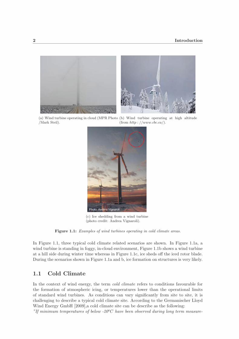
(a) Wind turbine operating in cloud (MPR Photo/Mark Steil).
(b) Wind turbine operating at high altitude(from http : //www.cbc.ca/).
(c) Ice shedding from a wind turbine(photo credit: Andrea Vignaroli).
Figure 1.1: Examples of wind turbines operating in cold climate areas.
In Figure 1.1, three typical cold climate related scenarios are shown. In Figure 1.1a, awind turbine is standing in foggy, in-cloud environment, Figure 1.1b shows a wind turbineat a hill side during winter time whereas in Figure 1.1c, ice sheds off the iced rotor blade.During the scenarios shown in Figure 1.1a and b, ice formation on structures is very likely.
1.1 Cold Climate
In the context of wind energy, the term cold climate refers to conditions favourable forthe formation of atmospheric icing, or temperatures lower than the operational limitsof standard wind turbines. As conditions can vary significantly from site to site, it ischallenging to describe a typical cold climate site. According to the Germanischer LloydWind Energy GmbH [2009],a cold climate site can be describe as the following:”If minimum temperatures of below -20oC have been observed during long term measure-
1.1 Cold Climate 3
ments (preferably ten years or more) on an average of more than nine days a year ora yearly mean temperature of less than 0 oC, the site is defined as a cold climate site.The nine-day criteria are fulfilled, if the temperature at the site remains below -20oC forone hour or more on the respective days. In this case, it has to be counted on specialrequirements for the wind turbine and the wind turbine shall be designed for cold climateconditions.”
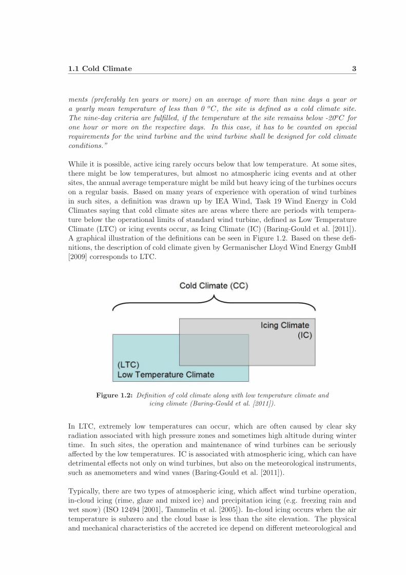
While it is possible, active icing rarely occurs below that low temperature. At some sites,there might be low temperatures, but almost no atmospheric icing events and at othersites, the annual average temperature might be mild but heavy icing of the turbines occurson a regular basis. Based on many years of experience with operation of wind turbinesin such sites, a definition was drawn up by IEA Wind, Task 19 Wind Energy in ColdClimates saying that cold climate sites are areas where there are periods with tempera-ture below the operational limits of standard wind turbine, defined as Low TemperatureClimate (LTC) or icing events occur, as Icing Climate (IC) (Baring-Gould et al. [2011]).A graphical illustration of the definitions can be seen in Figure 1.2. Based on these defi-nitions, the description of cold climate given by Germanischer Lloyd Wind Energy GmbH[2009] corresponds to LTC.
Figure 1.2: Definition of cold climate along with low temperature climate andicing climate (Baring-Gould et al. [2011]).
In LTC, extremely low temperatures can occur, which are often caused by clear skyradiation associated with high pressure zones and sometimes high altitude during wintertime. In such sites, the operation and maintenance of wind turbines can be seriouslyaffected by the low temperatures. IC is associated with atmospheric icing, which can havedetrimental effects not only on wind turbines, but also on the meteorological instruments,such as anemometers and wind vanes (Baring-Gould et al. [2011]).
Typically, there are two types of atmospheric icing, which affect wind turbine operation,in-cloud icing (rime, glaze and mixed ice) and precipitation icing (e.g. freezing rain andwet snow) (ISO 12494 [2001], Tammelin et al. [2005]). In-cloud icing occurs when the airtemperature is subzero and the cloud base is less than the site elevation. The physicaland mechanical characteristics of the accreted ice depend on different meteorological and
4 Introduction
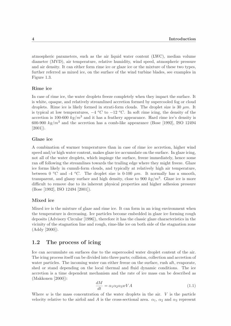
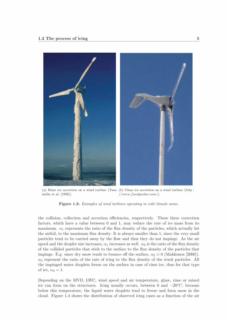
atmospheric parameters, such as the air liquid water content (LWC), median volumediameter (MVD), air temperature, relative humidity, wind speed, atmospheric pressureand air density. It can either form rime ice or glaze ice or the mixture of these two types,further referred as mixed ice, on the surface of the wind turbine blades, see examples inFigure 1.3.
Rime ice
In case of rime ice, the water droplets freeze completely when they impact the surface. Itis white, opaque, and relatively streamlined accretion formed by supercooled fog or clouddroplets. Rime ice is likely formed in strati-form clouds. The droplet size is 30 μm. Itis typical at low temperatures, −4 oC to −12 oC. In soft rime icing, the density of theaccretion is 100-600 kg/m3 and it has a feathery appearance. Hard rime ice’s density is600-900 kg/m3 and the accretion has a comb-like appearance (Bose [1992], ISO 12494[2001]).
Glaze ice
A combination of warmer temperatures than in case of rime ice accretion, higher windspeed and/or high water content, makes glaze ice accumulate on the surface. In glaze icing,not all of the water droplets, which impinge the surface, freeze immediately, hence someran off following the streamlines towards the trailing edge where they might freeze. Glazeice forms likely in cumuli-form clouds, and typically at relatively high air temperature,between 0 oC and -4 oC. The droplet size is 0-100 μm. It normally has a smooth,transparent, and glassy surface and high density, close to 900 kg/m3. Glaze ice is moredifficult to remove due to its inherent physical properties and higher adhesion pressure(Bose [1992], ISO 12494 [2001]).
Mixed ice
Mixed ice is the mixture of glaze and rime ice. It can form in an icing environment whenthe temperature is decreasing. Ice particles become embedded in glaze ice forming roughdeposits (Advisory Circular [1996]), therefore it has the classic glaze characteristics in thevicinity of the stagnation line and rough, rime-like ice on both side of the stagnation zone(Addy [2000]).
1.2 The process of icing
Ice can accumulate on surfaces due to the supercooled water droplet content of the air.The icing process itself can be divided into three parts; collision, collection and accretion ofwater particles. The incoming water can either freeze on the surface, rush aft, evaporate,shed or stand depending on the local thermal and fluid dynamic conditions. The iceaccretion is a time dependent mechanism and the rate of ice mass can be described as(Makkonen [2000]):
dM
dt= α1α2α3wV A (1.1)
Where w is the mass concentration of the water droplets in the air. V is the particlevelocity relative to the airfoil and A is the cross-sectional area. α1, α2 and α3 represent
1.2 The process of icing 5
(a) Rime ice accretion on a wind turbine (Tam-melin et al. [1998]).
(b) Glaze ice accretion on a wind turbine (http ://www.fundysolar.com/).
Figure 1.3: Examples of wind turbines operating in cold climate areas.
the collision, collection and accretion efficiencies, respectively. These three correctionfactors, which have a value between 0 and 1, may reduce the rate of ice mass from itsmaximum. α1 represents the ratio of the flux density of the particles, which actually hitthe airfoil, to the maximum flux density. It is always smaller than 1, since the very smallparticles tend to be carried away by the flow and thus they do not impinge. As the airspeed and the droplet size increases, α1 increases as well. α2 is the ratio of the flux densityof the collided particles that stick to the surface to the flux density of the particles thatimpinge. E.g. since dry snow tends to bounce off the surface, α2 � 0 (Makkonen [2000]).α3 represent the ratio of the rate of icing to the flux density of the stuck particles. Allthe impinged water droplets freeze on the surface in case of rime ice, thus for that typeof ice, α3 = 1.
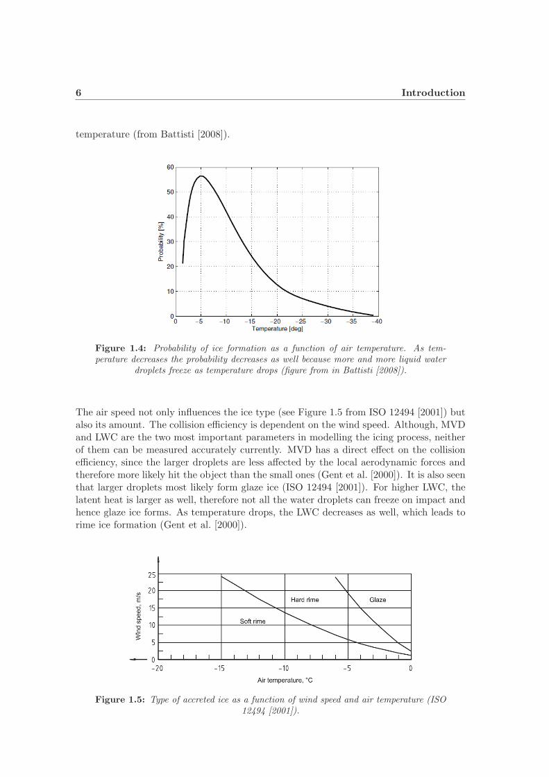
Depending on the MVD, LWC, wind speed and air temperature, glaze, rime or mixedice can form on the structures. Icing usually occurs, between 0 and −20oC, becausebelow this temperature, the liquid water droplets tend to freeze and form snow in thecloud. Figure 1.4 shows the distribution of observed icing cases as a function of the air
6 Introduction
temperature (from Battisti [2008]).
Figure 1.4: Probability of ice formation as a function of air temperature. As tem-perature decreases the probability decreases as well because more and more liquid water
droplets freeze as temperature drops (figure from in Battisti [2008]).
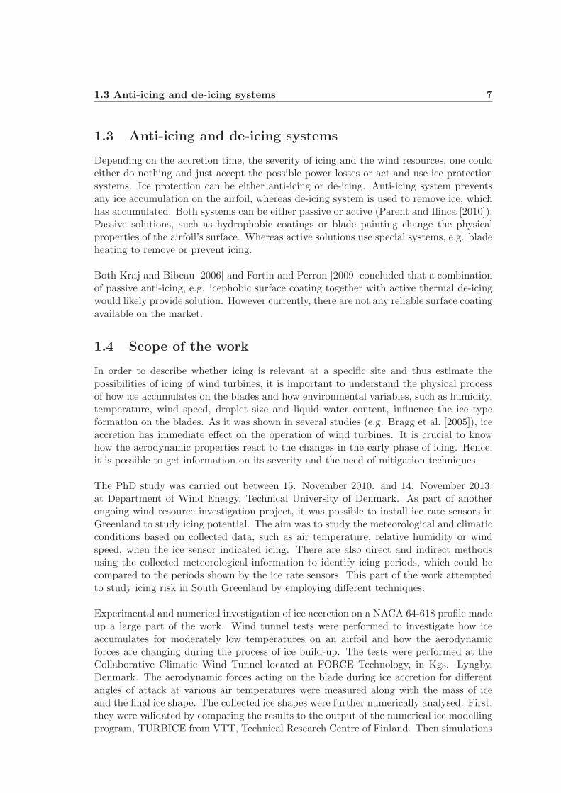
The air speed not only influences the ice type (see Figure 1.5 from ISO 12494 [2001]) butalso its amount. The collision efficiency is dependent on the wind speed. Although, MVDand LWC are the two most important parameters in modelling the icing process, neitherof them can be measured accurately currently. MVD has a direct effect on the collisionefficiency, since the larger droplets are less affected by the local aerodynamic forces andtherefore more likely hit the object than the small ones (Gent et al. [2000]). It is also seenthat larger droplets most likely form glaze ice (ISO 12494 [2001]). For higher LWC, thelatent heat is larger as well, therefore not all the water droplets can freeze on impact andhence glaze ice forms. As temperature drops, the LWC decreases as well, which leads torime ice formation (Gent et al. [2000]).
Figure 1.5: Type of accreted ice as a function of wind speed and air temperature (ISO12494 [2001]).
1.3 Anti-icing and de-icing systems 7
1.3 Anti-icing and de-icing systems
Depending on the accretion time, the severity of icing and the wind resources, one couldeither do nothing and just accept the possible power losses or act and use ice protectionsystems. Ice protection can be either anti-icing or de-icing. Anti-icing system preventsany ice accumulation on the airfoil, whereas de-icing system is used to remove ice, whichhas accumulated. Both systems can be either passive or active (Parent and Ilinca [2010]).Passive solutions, such as hydrophobic coatings or blade painting change the physicalproperties of the airfoil’s surface. Whereas active solutions use special systems, e.g. bladeheating to remove or prevent icing.
Both Kraj and Bibeau [2006] and Fortin and Perron [2009] concluded that a combinationof passive anti-icing, e.g. icephobic surface coating together with active thermal de-icingwould likely provide solution. However currently, there are not any reliable surface coatingavailable on the market.
1.4 Scope of the work
In order to describe whether icing is relevant at a specific site and thus estimate thepossibilities of icing of wind turbines, it is important to understand the physical processof how ice accumulates on the blades and how environmental variables, such as humidity,temperature, wind speed, droplet size and liquid water content, influence the ice typeformation on the blades. As it was shown in several studies (e.g. Bragg et al. [2005]), iceaccretion has immediate effect on the operation of wind turbines. It is crucial to knowhow the aerodynamic properties react to the changes in the early phase of icing. Hence,it is possible to get information on its severity and the need of mitigation techniques.
The PhD study was carried out between 15. November 2010. and 14. November 2013.at Department of Wind Energy, Technical University of Denmark. As part of anotherongoing wind resource investigation project, it was possible to install ice rate sensors inGreenland to study icing potential. The aim was to study the meteorological and climaticconditions based on collected data, such as air temperature, relative humidity or windspeed, when the ice sensor indicated icing. There are also direct and indirect methodsusing the collected meteorological information to identify icing periods, which could becompared to the periods shown by the ice rate sensors. This part of the work attemptedto study icing risk in South Greenland by employing different techniques.
Experimental and numerical investigation of ice accretion on a NACA 64-618 profile madeup a large part of the work. Wind tunnel tests were performed to investigate how iceaccumulates for moderately low temperatures on an airfoil and how the aerodynamicforces are changing during the process of ice build-up. The tests were performed at theCollaborative Climatic Wind Tunnel located at FORCE Technology, in Kgs. Lyngby,Denmark. The aerodynamic forces acting on the blade during ice accretion for differentangles of attack at various air temperatures were measured along with the mass of iceand the final ice shape. The collected ice shapes were further numerically analysed. First,they were validated by comparing the results to the output of the numerical ice modellingprogram, TURBICE from VTT, Technical Research Centre of Finland. Then simulations

8 Introduction
with Ansys Fluent were conducted to analyse the impact of ice accretion on the flowbehaviour and the aerodynamic characteristics of the iced airfoil at different wind speeds.
The paper of Seifert and Richert [1997] is very often cited. This paper contains verypromising iced lift curve transformation method, which is tested during the PhD study andthe results are compared to the outcome of the experimental and numerical investigation.
Chapter 2
Risk of icing in South-Greenlandfor wind energy
Remote locations all over the world are facing similar issues when it comes to powersources. The scattered cities and villages and also the isolated research stations (e.g.Summit Station in Greenland or McMurdo Station in the Antarctica) do not have directconnection to central infrastructure, such as pipelines and electricity grids. Historically,diesel and other fossil fuel based generators provided the only feasible solution in thepast. However, increasing fuel costs and the worldwide ambitions to reduce the use ofthese energy sources led to a greater reliance on local and sustainable forms of energy(IEA-RETD [2012]).
Greenland’s many small village communities with their own local electrical grids and thelarge geographical distances mean that the cost of energy production varies widely. Inlarger cities, such as Nuuk or Qaqortoq with a relatively high consumption and accessto hydro-power, the cost of energy is lower, whereas in small, remote villages, it can beextremely high.
The electrical grid system of Greenland is built of small and isolated grids where almosteach single town or village is responsible for its own power supply. They usually are notconnected to each other due to the great distance, hence there is no central grid. Thisstructure results in high cost of backup capacity, energy storage and fuel transport (Vil-lumsen et al. [2009]). Energy storage in the small isolated villages is a large challenge,because the consumption usually is much lower than e.g. the energy production of amodern wind turbine.
In the recent years, to fulfill the renewable energy usage targets and to reduce the de-pendency of diesel fuel, the possibilities of implementing wind turbines into the alreadyexisting energy system have been investigated. Since the yearly mean temperature inGreenland is approximately −1oC, it can be considered as cold climate site accordingto the definitions of Germanischer Lloyd Wind Energy GmbH [2009]. Icing is worthy ofinvestigation to determine the threat to structures and wind turbines. Therefore as a partof the project ice rate sensors were installed in two locations in South Greenland to learnmore about the relevance of icing events.
10 Risk of icing in South-Greenland for wind energy
2.1 Introduction to risk of icing in Greenland
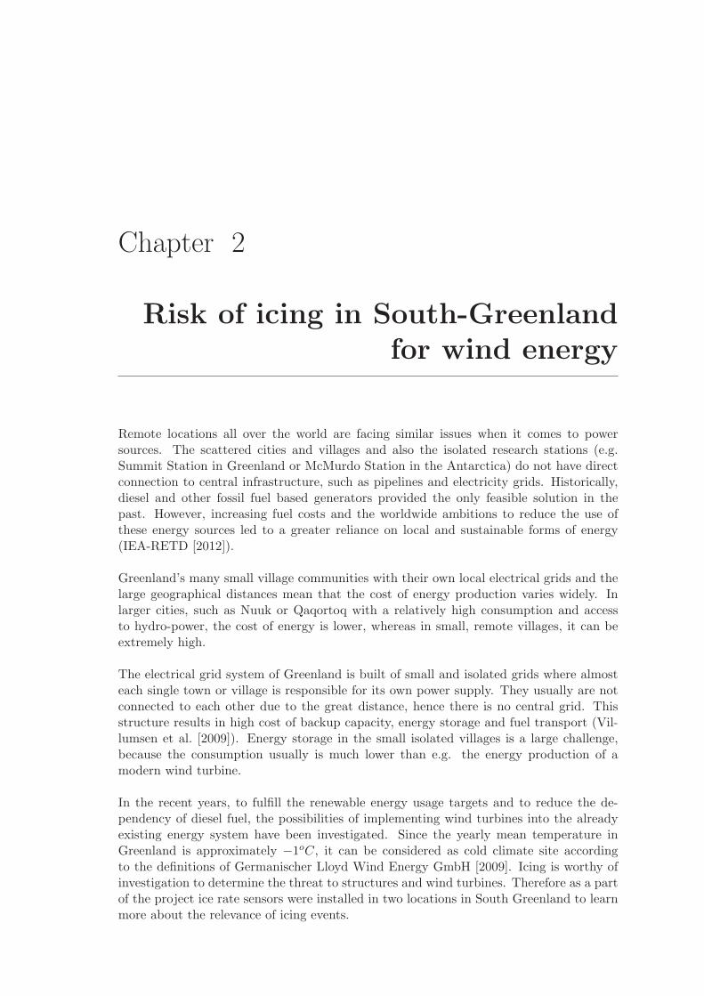
Since most parts of Greenland can be classified as cold climate locations, icing potentialshould be investigated before installing wind turbines. However, there have been no re-ports of detrimental icing of power lines or other structures in the inhabited areas. InFigure 2.1, a 6 kW Proven wind turbine can be seen, which was installed at SummitStation, in the middle of the icecap in Greenland. The severity of the rime icing was un-expected1. It accreted during very light wind periods, when the turbine was not operationand therefore could not shed of the particles.
Figure 2.1: Iced 6kW Proven turbine at Summit Station,in Greenland. This level of icing reduces power output by
80 % or greater. (Dahl [2009])
Historically, the towns are located in sheltered places in Greenland, i.e. wind speedis quite moderate. If wind energy were introduced into the local power system, theturbine(s) would probably be located at elevated sites, where the wind resources are morefavourable. These sites are not as sheltered, therefore the structures will likely have towithstand harsher environmental conditions, especially during winter.
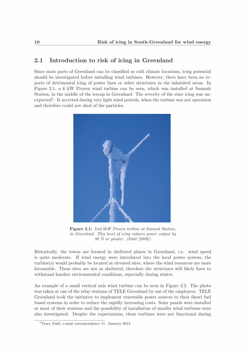
An example of a small vertical axis wind turbine can be seen in Figure 2.2. The photowas taken at one of the relay stations of TELE Greenland by one of the employees. TELEGreenland took the initiative to implement renewable power sources to their diesel fuelbased systems in order to reduce the rapidly increasing costs. Solar panels were installedat most of their stations and the possibility of installation of smaller wind turbines werealso investigated. Despite the expectations, these turbines were not functional during
1Tracy Dahl, e-mail correspondence 11. January 2013
2.1 Introduction to risk of icing in Greenland 11
winter due to the massive amount of ice, which accreted on them, as it is seen in Figure2.2.
Figure 2.2: A small vertical axis wind turbine located atone of the relay stations in Greenland (photo credit: TELE
Greenland).
These examples indicate that icing is a real treat to wind turbines in Greenland, and there-fore thorough investigation of the icing potential is needed as an additional feature to thewind resource studies. In 2003, Nordic Energy Research, ECON (Denmark) and Institutefor Energy Technology (Norway) started a project on establishment of community-basedrenewable energy and hydrogen (RE/H2) systems in the West Nordic Region. As a partof this project, wind energy monitoring was carried in Nanortalik, South Greenland. Forthis purpose a 50 m tall meteorological mast was erected in the town (Ulleberg and Mo-erkved [2008]). The station was collecting data for four years, and it was reported thatonly 2 % of data was missing due to icing (Aakervik [2011]). An icing event was indicated,when 5 or more consecutive wind direction measurements in a 10 minutes period wereidentical and the temperature was below 3 oC Laakso et al. [2009]. This means, that thewind vanes were iced as a block and they were not able to move.
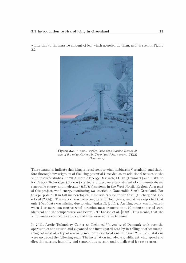
In 2011, Arctic Technology Center at Technical University of Denmark took over theoperation of the station and expanded the investigated area by installing another meteo-rological mast at a top of a nearby mountain (see locations in Figure 2.3). Both stationswere upgraded the following year. The installation included e.g. different wind speed anddirection sensors, humidity and temperature sensors and a dedicated ice rate sensor.
12 Risk of icing in South-Greenland for wind energy
Figure 2.3: Location of the stations in South-Greenland. One of the stations is locatedat sea level on the island of Nanortalik whereas the other one is on the top of a hill
approximately 900 m above sea level on the nearby island, Sermersooq.
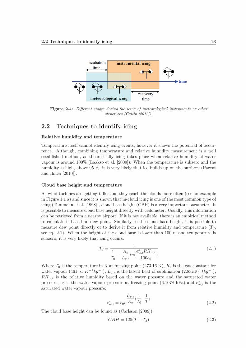
However, it is difficult to detect icing and its severity. There are different direct andindirect techniques to identify icing events (Carlsson [2009]). Direct techniques are e.g.cameras and ice detectors. Indirect technique is to investigate the climatic and mete-orological variables collected from the studied sites, such as wind speed and direction,temperature, relative humidity, air temperature and if available dew point and cloud baseheight. Using these parameters, it is possible to estimate the existence of icing (Fikkeet al. [2006]). Figure 2.4 shows clear difference between the two different types of ic-ing event, i.e. meteorological and instrumental icing. Meteorological icing is a periodwhen meteorological conditions favour ice build-up, whereas during instrumental icing,instrument and structures are covered by ice and icing has detrimental effect on theirfunctioning (Baring-Gould et al. [2011]).
2.2 Techniques to identify icing 13
Figure 2.4: Different stages during the icing of meteorological instruments or otherstructures (Cattin [2012]).
2.2 Techniques to identify icing
Relative humidity and temperature
Temperature itself cannot identify icing events, however it shows the potential of occur-rence. Although, combining temperature and relative humidity measurement is a wellestablished method, as theoretically icing takes place when relative humidity of watervapour is around 100% (Laakso et al. [2009]). When the temperature is subzero and thehumidity is high, above 95 %, it is very likely that ice builds up on the surfaces (Parentand Ilinca [2010]).
Cloud base height and temperature
As wind turbines are getting taller and they reach the clouds more often (see an examplein Figure 1.1 a) and since it is shown that in-cloud icing is one of the most common type oficing (Tammelin et al. [1998]), cloud base height (CBH) is a very important parameter. Itis possible to measure cloud base height directly with ceilometer. Usually, this informationcan be retrieved from a nearby airport. If it is not available, there is an empirical methodto calculate it based on dew point. Similarly to the cloud base height, it is possible tomeasure dew point directly or to derive it from relative humidity and temperature (Td,see eq. 2.1). When the height of the cloud base is lower than 100 m and temperature issubzero, it is very likely that icing occurs.
Td =1
1
T0− Rv
Lv,sln(
esw,iRHw,i
100e0)
(2.1)
Where T0 is the temperature in K at freezing point (273.16 K), Rv is the gas constant forwater vapour (461.51 K−1kg−1), Lv,s is the latent heat of sublimation (2.83x10⁶Jkg−1),RHw,i is the relative humidity based on the water pressure and the saturated waterpressure, e0 is the water vapour pressure at freezing point (6.1078 hPa) and esw,i is thesaturated water vapour pressure:
esw,i = e0e
Lv,s
Rv(1
T0−1
T)
(2.2)
The cloud base height can be found as (Carlsson [2009]):
CBH = 125(T − Td) (2.3)
14 Risk of icing in South-Greenland for wind energy
Where T is the air temperature at the ground.
Wind speed monitored by heated and unheated anemometers
Comparing the results of an unheated and heated anemometer is a very simple but roughestimation of icing. It is not possible to estimate the amount of ice, which builds up onthe sensors with this technique. If the output of the two sensors is different, it can beassumed that ice accreted on the unheated one. The unheated anemometer could eithershow lower wind speed than the heated one or be completely frozen and give values closeto zero (Ilinca [2011]). There is not any standard on the difference between the twooutputs, but the literature suggests values from 5 % to 20 % (Parent and Ilinca [2010]).An estimate of the standard maximum error between the two anemometers can be foundby investigating the differences in the data from summer period when icing is unlikely tooccur.
Frozen anemometer
If there are not any heated anemometers installed on the meteorological station, icingevents could be identified by low temperature and very slow or stand still anemometers.This is, however, an underestimation of the icing potential, since ice build-up does notnecessary stop the instruments completely.
Wind vanes
It is thorough to install both heated and unheated wind vanes not only to identify theicing periods but also to be able to monitor the wind direction during icing event whenthe unheated instruments might be malfunctioning. If there are big differences in thewind direction measured by the two sensors, it might be due to icing. If there is onlyunheated wind vane installed on the meteorological mast, it can be assumed that theequipment is iced, when five or more consecutive wind direction measurements in a 10minute series are identical and the temperature is subzero [Aakervik, 2011]. This methodonly provides an information about the period when significant amount of ice sticks onthe surface and the wind vanes are not able to turn. This gives underestimation of theicing period because even a very small amount of ice has large effect on the performanceof the sensors [Laakso et al., 2009]. However, if the STD is zero for longer period due tolow wind speed, this method could, in the contrary, overestimate the icing event.
Cameras
In the last couple of years, the quality of the images has improved significantly hencecameras can capture icing events quite well on stand still structures [Cattin, 2012]. If thecamera is installed on a meteorological mast and pointing towards one of the instruments,it can give a good solution to capturing icing periods.
In case of monitoring icing of wind turbine blades, the cameras can be placed either on thespinner of the rotor or on the nacelle. In case of the first method, the camera captures thesame blade and rotates along with it and hence it is exposed to harsh weather conditions.Due to the flat angle of view, it could be difficult or even impossible to see the tip of

2.3 Sites and installations 15
the blade. In case of placing the camera on the nacelle, the blade is captured by motiondetection when it appears in the image. The camera is less exposed, but it is neitherthe same blade on the images nor possible to see the whole blade either. During nightsand foggy periods, when icing is more likely, the quality of images decreases dramatically.Another disadvantage of using digital cameras is the lack of automatic processing.
Ice detectors
Currently there are several types of ice detectors on the market (see Homola et al. [2006]),but none of them are reliable for heavy icing conditions. Changes of some properties,such as mass, reflective properties or electrical/thermal conductivity (Ilinca [2011]) canbe detected by sensors.
In Nanortalik, an optical ice detector, a HoloOptics T44 ice rate sensor, which emitsinfra-red light towards a reflective surface, was installed in 2011. It interprets variationsbetween emitted light and light received by the photo sensor (HoloOptics manual). Themain parts of the HoloOptics T44 are four arms and a probe. The arms contain an IRemitter and a modular detector. The probe has a reflective surface that can reflect theradiation emitted by the arms back to the detectors as long as there is no ice accretion onit (HoloOptics manual). The presence of icing is indicated when an approximately 0.01-0.03 mm thick ice layer covers the 85-95 % of the probe surface. In that case, internalheating turns on and de-ices the sensor. The sensor monitors the number of indicationsand also the time necessary for de-icing, which could give good information about the icerate, Ri (g/mh). Based on the number of indications:
Ri = 0.76e0.027∗Ai (2.4)
Where Ai is the number of indications per hour. And based on the indication time:
Ri = 0.94 ∗ e7.6∗Ti/Ttot (2.5)
Where Ti is the indication time during the measurement period and Ttot is the measure-ment period length (recommended to be 3600 s).
2.3 Sites and installations
The two sites where the meteorological masts were installed are shown in Figure 2.3. Twodata collecting periods can be distinguished at the test site in Nanortalik. In the firstperiod, the data was collected with the old set-up as a part of the ’Vest-Nordensamarbejde’project, whereas in the second period, the data was collected with the new set-up, whichwas installed in summer of 2012. However, in 2011 when the ’Vest-Nordensamarbejde’project ended and DTU overtook the operation of the mast, a HoloOptics ice rate sensorand a relative humidity sensor were added to the old set-up as an additional feature.Before that, the humidity data was provided by the nearby heliport’s station. Thisstation also provides 10 minutes data series and due to the relatively flat landscape andthe short distance between the two locations, no corrections are necessary. The installedinstruments are listed in Table 2.1 for both set-ups.
16 Risk of icing in South-Greenland for wind energy
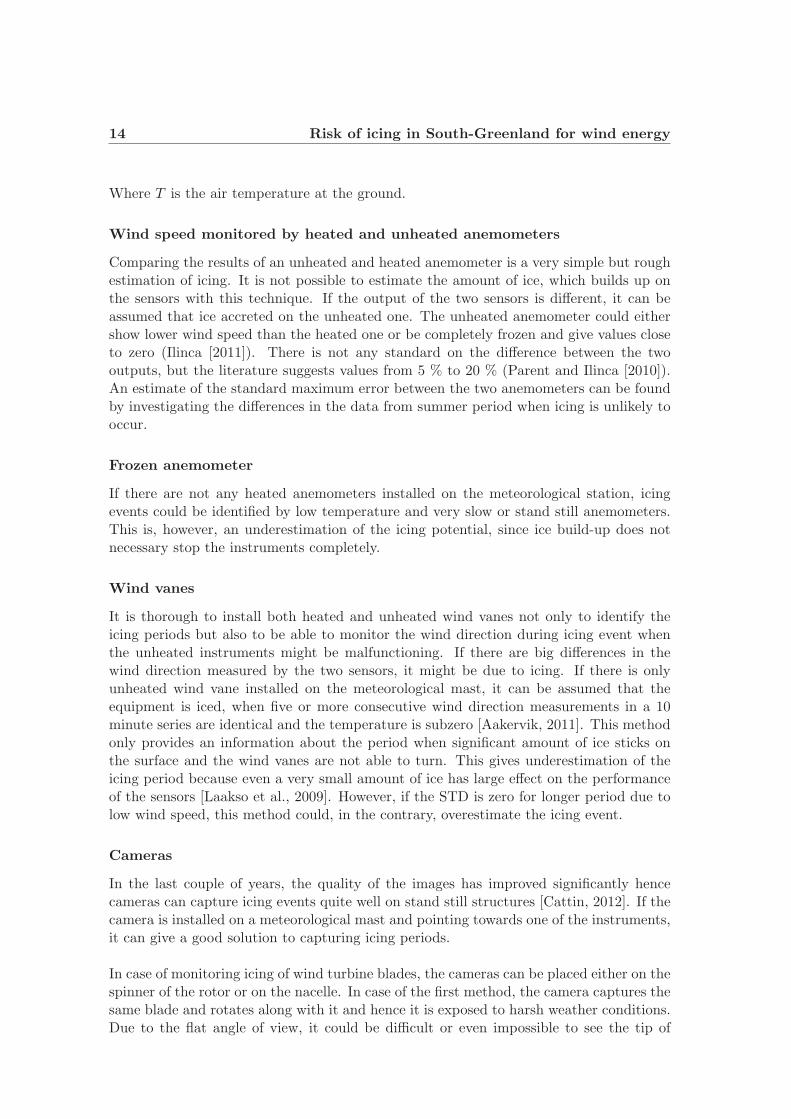
Table 2.1: Set-up of the meteorological mast installed in Nanortalik, SouthGreenland.
Old set-up
Type Brand H (m)Anemometer NRG 40 48.8Anemometer Risoe P2546A 48.8Anemometer NRG 40 30Anemometer NRG 40 10Anemometer NRG HAE IceFree 3 43.8Wind vane NRG HVE IceFree 3 40.8Wind vane NRG 200P 41.4Air temp. NRG 110S 3Humidity RH5X 3
Ice rate sensor HoloOptics T44 4
New set-up
Type Brand H (m)Sonic anemometer Metek Usonic 3D Heated 50
Anemometer Risoe P2546A 49Wind vane NRG 200P 49Anemometer Risoe P2546A 30Anemometer Risoe P2546A 10Wind vane NRG 200P 10Pyranometer Hekseflux LP02-05 5Ice rate sensor HoloOptics T44 5
Air temp. NRG 110S 3Air temp. Vaisala HMP155 3Humidity Vaisala HMP155 3Humidity NRG RH-X5 3
Potential temp. 48.5-5m
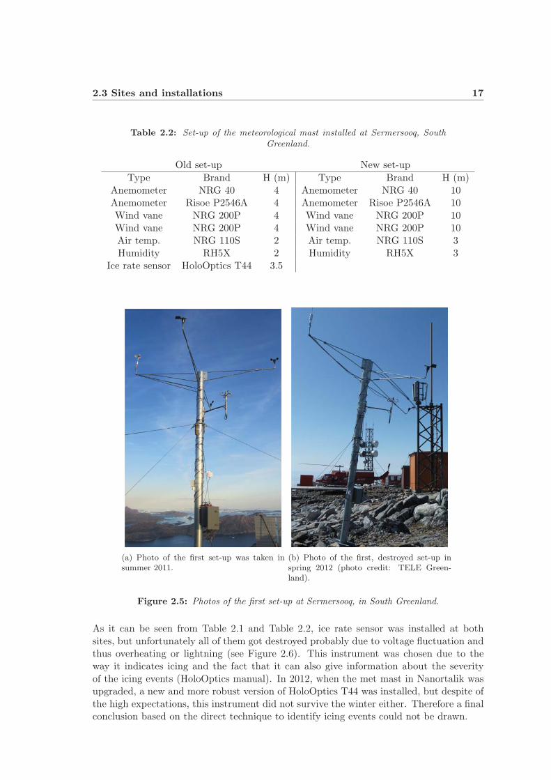
The top of a mountain in the nearby island, Sermersooq was chosen based on informationon possible icing events from the local telecommunication company, TELE Greenland thathas a relay station located there and hence it was possible to get assistance from themduring both installation and operation. There were also two different set-ups installed atthis test site. In the first year a smaller, 4 m tall mast was erected with the purpose to seewhether icing was a real treat there. The connection to the station was lost in February2012 and it turned out that the set-up was destroyed during a winter storm, see photos ofthe set-up after installation and after winter in Figure 2.5 a and Figure 2.5 b, respectively.In the summer of 2012, a tower with an extension to 10 m was installed with extra guywires added for security, but this setup also could not withstand the harsh winter.
2.3 Sites and installations 17
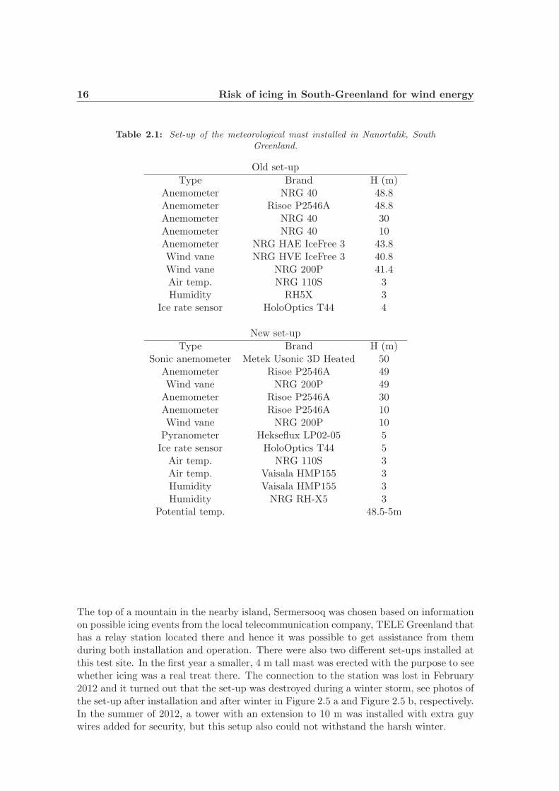
Table 2.2: Set-up of the meteorological mast installed at Sermersooq, SouthGreenland.
Old set-up New set-up
Type Brand H (m) Type Brand H (m)Anemometer NRG 40 4 Anemometer NRG 40 10Anemometer Risoe P2546A 4 Anemometer Risoe P2546A 10Wind vane NRG 200P 4 Wind vane NRG 200P 10Wind vane NRG 200P 4 Wind vane NRG 200P 10Air temp. NRG 110S 2 Air temp. NRG 110S 3Humidity RH5X 2 Humidity RH5X 3
Ice rate sensor HoloOptics T44 3.5
(a) Photo of the first set-up was taken insummer 2011.
(b) Photo of the first, destroyed set-up inspring 2012 (photo credit: TELE Green-land).
Figure 2.5: Photos of the first set-up at Sermersooq, in South Greenland.
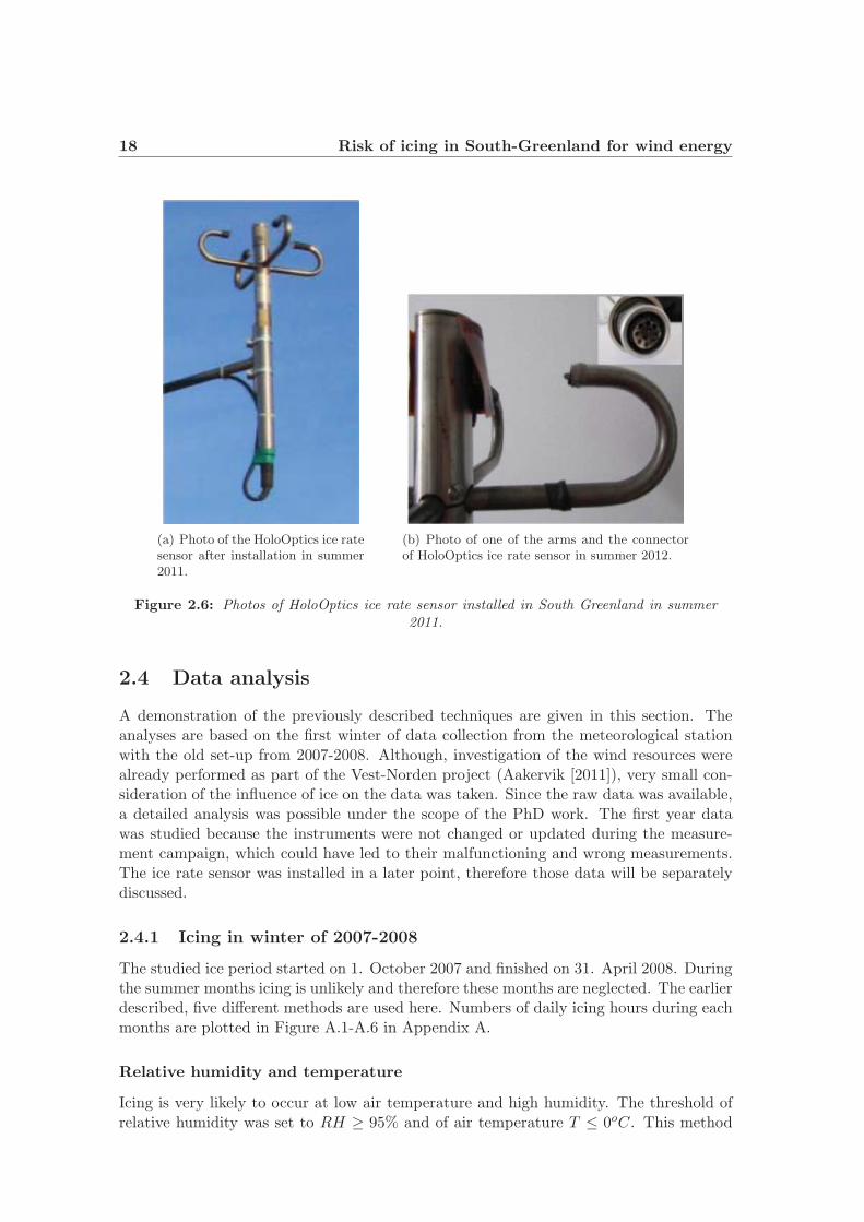
As it can be seen from Table 2.1 and Table 2.2, ice rate sensor was installed at bothsites, but unfortunately all of them got destroyed probably due to voltage fluctuation andthus overheating or lightning (see Figure 2.6). This instrument was chosen due to theway it indicates icing and the fact that it can also give information about the severityof the icing events (HoloOptics manual). In 2012, when the met mast in Nanortalik wasupgraded, a new and more robust version of HoloOptics T44 was installed, but despite ofthe high expectations, this instrument did not survive the winter either. Therefore a finalconclusion based on the direct technique to identify icing events could not be drawn.
18 Risk of icing in South-Greenland for wind energy
(a) Photo of the HoloOptics ice ratesensor after installation in summer2011.
(b) Photo of one of the arms and the connectorof HoloOptics ice rate sensor in summer 2012.
Figure 2.6: Photos of HoloOptics ice rate sensor installed in South Greenland in summer2011.
2.4 Data analysis
A demonstration of the previously described techniques are given in this section. Theanalyses are based on the first winter of data collection from the meteorological stationwith the old set-up from 2007-2008. Although, investigation of the wind resources werealready performed as part of the Vest-Norden project (Aakervik [2011]), very small con-sideration of the influence of ice on the data was taken. Since the raw data was available,a detailed analysis was possible under the scope of the PhD work. The first year datawas studied because the instruments were not changed or updated during the measure-ment campaign, which could have led to their malfunctioning and wrong measurements.The ice rate sensor was installed in a later point, therefore those data will be separatelydiscussed.
2.4.1 Icing in winter of 2007-2008
The studied ice period started on 1. October 2007 and finished on 31. April 2008. Duringthe summer months icing is unlikely and therefore these months are neglected. The earlierdescribed, five different methods are used here. Numbers of daily icing hours during eachmonths are plotted in Figure A.1-A.6 in Appendix A.
Relative humidity and temperature
Icing is very likely to occur at low air temperature and high humidity. The threshold ofrelative humidity was set to RH ≥ 95% and of air temperature T ≤ 0oC. This method
2.4 Data analysis 19
implied 112 hours of icing in 16 days throughout the investigated 7 months. See plot ofthe daily icing hours for each month in Figure A.2.
Cloud base height and temperature
In-cloud icing is one of the main reasons for reduction of power production of wind turbines(Tammelin et al. [1998]). Low laying clouds accompanied by low air temperature causehigh risk of icing. The threshold of cloud base height was 100 m, which gave 188 hoursof possible icing in 29 days. A plot of the daily icing hours for each winter month duringthe investigated 7 months can be seen in Figure A.2.
Heated and unheated anemometer
This station was equipped with both heated and unheated anemometers, which gave arare opportunity to compare their output. A standard, �U = 0.7m/s offset was foundbetween the measurements taken by the two different anemometers. If the difference wassignificantly higher than this offset, icing was likely to happen. The threshold was set to�U = 1.4m/s, in order to neglect the small differences caused by the measurement errorsor other unexpected issues. There were no conditions set for temperature, because as itwas also shown in Figure 2.4, instrumental icing also exists during recovery time, andhence it is possible that the air temperature is above zero and icing is still effecting themeasurements in this period. In total, 446 icing hours in 56 days fulfilled this requirement,see Figure A.3.
Frozen anemometer
If an unheated anemometer is frozen and stops, it cannot measure the wind speed. How-ever this scenario rarely happens. With this method, it is not possible to identify theincubation and recovery period, but only the events, when the anemometer was not mov-ing. The unheated anemometer was frozen for 27 hours, in 5 days during the investigated7 months see Figure A.4.
Wind vane and temperature
As it was explained earlier, the standard deviation of the wind vane measurements couldalso indicate icing. Due to the error filtering of the data some of the recordings hadto be removed and therefore some compromises had to be made. Parent and Ilinca[2010] suggested that the combination of six consecutive 10 minute measurements of zerostandard deviation (STD) and subzero temperature implies to the presence of ice on thevanes. In this study, these requirements were changed. A limit of two measurements ofzero STD in 30 minutes would raise a flag and minimum six of these indications per daywould be considered as icing day. This criteria gave 108 days when icing event might haveoccurred based on the unheated vane (see Figure A.5) and 17 days based on the heatedone (see Figure A.6).
Example - April 2008.
In Figure 2.7, the 10 minute wind speed data for April 2008 is plotted for both heatedand unheated anemometers. The earlier mentioned offset is visible on this plot. It can
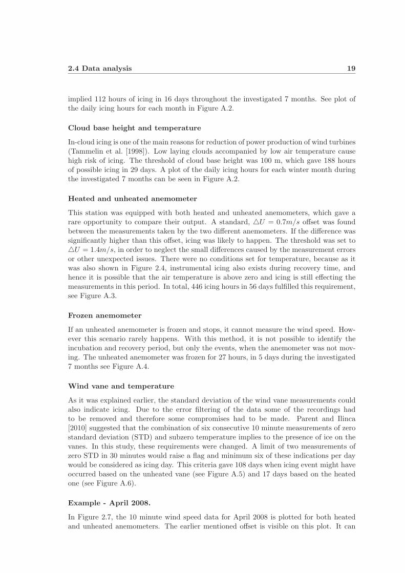
20 Risk of icing in South-Greenland for wind energy
also be noticed that in the beginning of the month the unheated anemometer was notmeasuring, i.e. it was probably frozen.
Figure 2.7: Wind speed based on 10 minutes measurements in April 2008. Thereare two periods marked with red circles when the unheated anemometer was not taking
measurements.
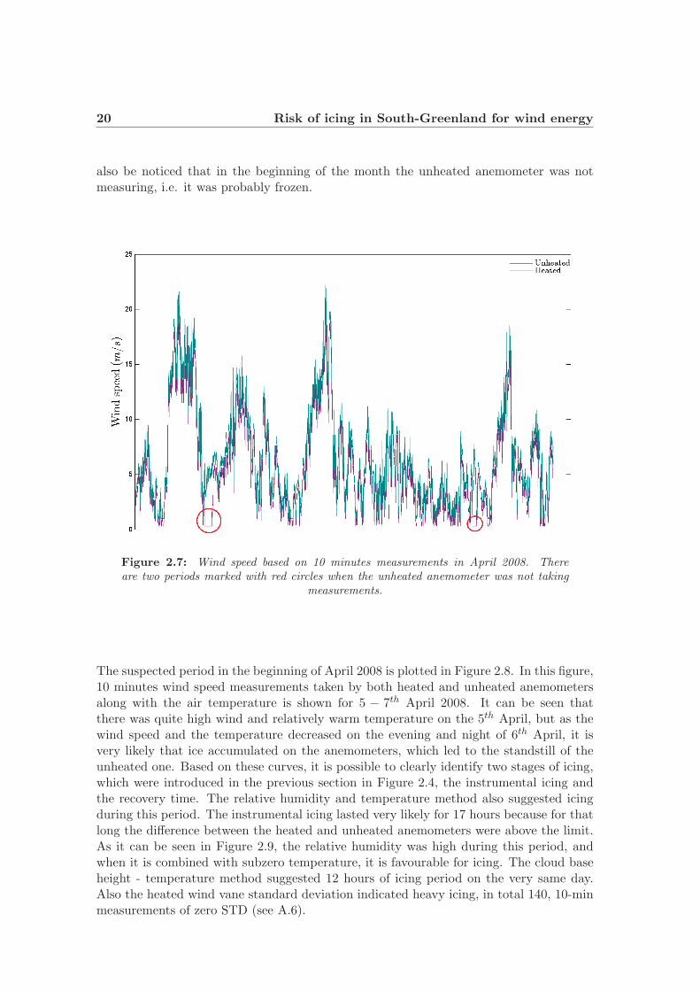
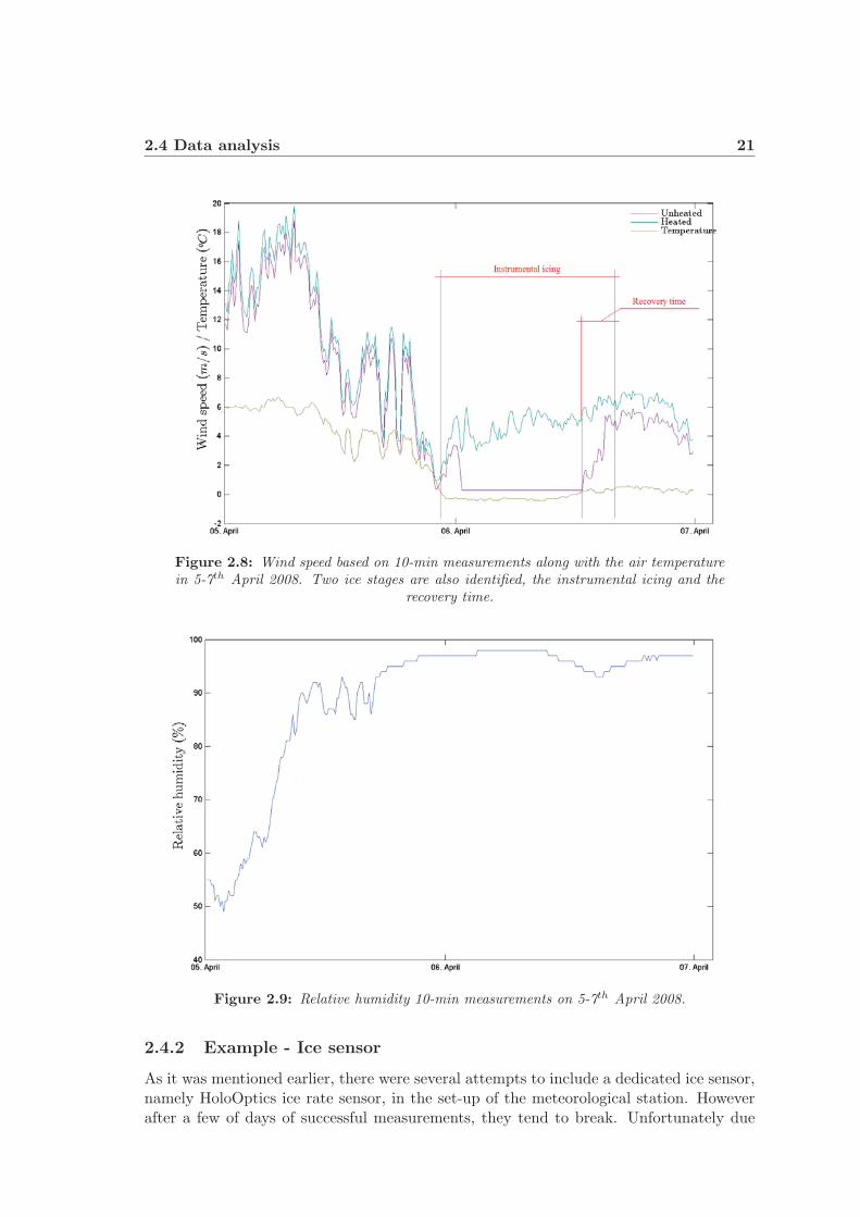
The suspected period in the beginning of April 2008 is plotted in Figure 2.8. In this figure,10 minutes wind speed measurements taken by both heated and unheated anemometersalong with the air temperature is shown for 5 − 7th April 2008. It can be seen thatthere was quite high wind and relatively warm temperature on the 5th April, but as thewind speed and the temperature decreased on the evening and night of 6th April, it isvery likely that ice accumulated on the anemometers, which led to the standstill of theunheated one. Based on these curves, it is possible to clearly identify two stages of icing,which were introduced in the previous section in Figure 2.4, the instrumental icing andthe recovery time. The relative humidity and temperature method also suggested icingduring this period. The instrumental icing lasted very likely for 17 hours because for thatlong the difference between the heated and unheated anemometers were above the limit.As it can be seen in Figure 2.9, the relative humidity was high during this period, andwhen it is combined with subzero temperature, it is favourable for icing. The cloud baseheight - temperature method suggested 12 hours of icing period on the very same day.Also the heated wind vane standard deviation indicated heavy icing, in total 140, 10-minmeasurements of zero STD (see A.6).
2.4 Data analysis 21
Figure 2.8: Wind speed based on 10-min measurements along with the air temperaturein 5-7th April 2008. Two ice stages are also identified, the instrumental icing and the
recovery time.
Figure 2.9: Relative humidity 10-min measurements on 5-7th April 2008.
2.4.2 Example - Ice sensor
As it was mentioned earlier, there were several attempts to include a dedicated ice sensor,namely HoloOptics ice rate sensor, in the set-up of the meteorological station. Howeverafter a few of days of successful measurements, they tend to break. Unfortunately due
22 Risk of icing in South-Greenland for wind energy
to the remote locations, it was not possible to investigate them right after these eventstherefore it was impossible to find out what had happened exactly.
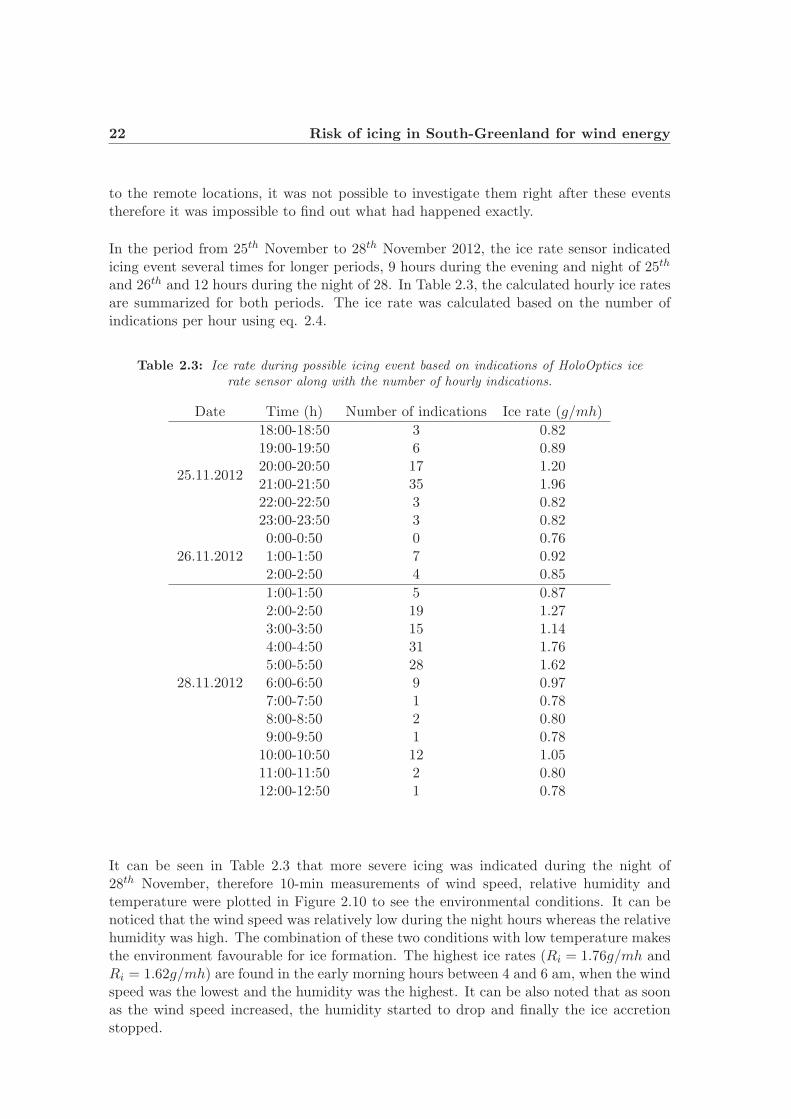
In the period from 25th November to 28th November 2012, the ice rate sensor indicatedicing event several times for longer periods, 9 hours during the evening and night of 25th
and 26th and 12 hours during the night of 28. In Table 2.3, the calculated hourly ice ratesare summarized for both periods. The ice rate was calculated based on the number ofindications per hour using eq. 2.4.
Table 2.3: Ice rate during possible icing event based on indications of HoloOptics icerate sensor along with the number of hourly indications.
Date Time (h) Number of indications Ice rate (g/mh)
25.11.2012
18:00-18:50 3 0.8219:00-19:50 6 0.8920:00-20:50 17 1.2021:00-21:50 35 1.9622:00-22:50 3 0.8223:00-23:50 3 0.82
26.11.20120:00-0:50 0 0.761:00-1:50 7 0.922:00-2:50 4 0.85
28.11.2012
1:00-1:50 5 0.872:00-2:50 19 1.273:00-3:50 15 1.144:00-4:50 31 1.765:00-5:50 28 1.626:00-6:50 9 0.977:00-7:50 1 0.788:00-8:50 2 0.809:00-9:50 1 0.78
10:00-10:50 12 1.0511:00-11:50 2 0.8012:00-12:50 1 0.78
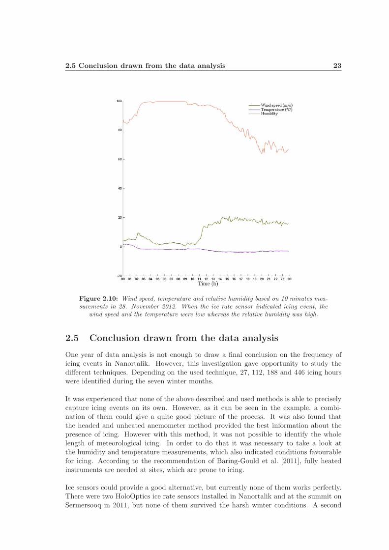
It can be seen in Table 2.3 that more severe icing was indicated during the night of28th November, therefore 10-min measurements of wind speed, relative humidity andtemperature were plotted in Figure 2.10 to see the environmental conditions. It can benoticed that the wind speed was relatively low during the night hours whereas the relativehumidity was high. The combination of these two conditions with low temperature makesthe environment favourable for ice formation. The highest ice rates (Ri = 1.76g/mh andRi = 1.62g/mh) are found in the early morning hours between 4 and 6 am, when the windspeed was the lowest and the humidity was the highest. It can be also noted that as soonas the wind speed increased, the humidity started to drop and finally the ice accretionstopped.
2.5 Conclusion drawn from the data analysis 23
Figure 2.10: Wind speed, temperature and relative humidity based on 10 minutes mea-surements in 28. November 2012. When the ice rate sensor indicated icing event, the
wind speed and the temperature were low whereas the relative humidity was high.
2.5 Conclusion drawn from the data analysis
One year of data analysis is not enough to draw a final conclusion on the frequency oficing events in Nanortalik. However, this investigation gave opportunity to study thedifferent techniques. Depending on the used technique, 27, 112, 188 and 446 icing hourswere identified during the seven winter months.
It was experienced that none of the above described and used methods is able to preciselycapture icing events on its own. However, as it can be seen in the example, a combi-nation of them could give a quite good picture of the process. It was also found thatthe headed and unheated anemometer method provided the best information about thepresence of icing. However with this method, it was not possible to identify the wholelength of meteorological icing. In order to do that it was necessary to take a look atthe humidity and temperature measurements, which also indicated conditions favourablefor icing. According to the recommendation of Baring-Gould et al. [2011], fully heatedinstruments are needed at sites, which are prone to icing.
Ice sensors could provide a good alternative, but currently none of them works perfectly.There were two HoloOptics ice rate sensors installed in Nanortalik and at the summit onSermersooq in 2011, but none of them survived the harsh winter conditions. A second

24 Risk of icing in South-Greenland for wind energy
attempt was made in 2012, when a more robust version was installed as a part of the newset-up in Nanortalik. Unfortunately, the connection to that specific instrument was lostafter a few of days of icing events, which indicates that it was also destroyed or its cablegot loose. However, it was possible to use the indicated icing period as a demonstrationcase. Quite severe ice accumulation was identified during the night of 28. November. Theresults could be validated by the high relative humidity, subzero temperature and lowwind speed measurements.
Recently a number of recommendations have been published about the proper installa-tion of meteorological test stations in the cold climate areas (e.g. Arbez et al. [2013]).Following these guidances, it is possible to minimize the detrimental effect of icing on themeasurements and also more precisely identify the icing events and even the ice rate.
The results and experiences suggest that icing is a threat in South-Greenland during peri-ods with low wind speed and high relative humidity combined with subzero temperature(or close to 0 oC). If the decision was made to install a wind turbine in a specific loca-tion, it is suggested to include a thorough investigation of risk of ice along with the windresource analysis.
Chapter 3
Experimental investigation of theeffect of ice on wind turbine
blades
Experimental investigation of icing of wind turbine blades can give a unique, hands-onexperience with phenomenon and issues that are difficult to investigate in full scale. Theexperiments described in this chapter were carried out in the Collaborative Climatic WindTunnel (CWT). Glaze, rime and mixed ice deposits were built up on a NACA 64-618 airfoilprofile and the aerodynamic responses were monitored during the accretion process.
This chapter gives an overview of the experimental investigation of the effect of ice build-up on airfoils and describes the ice accretion tests performed in the CWT during thePhD work. A detailed description of the wind tunnel set-up, including e.g. the testfacility itself, the spray-system and the force and torque transducers, is also presentedhere. Since the values measured by the force and torque transducers are in voltage (V ),it was necessary to calibrate them to Newton (N), therefore the data calibration is alsoexplained.
3.1 Introduction to wind tunnel testing
Aircraft ice accretion has been a large problem since the very early years of flying (Gentet al. [2000]). It gives a good basis (i.e. Bragg et al. [2005], Blumenthal et al. [2006] orBragg et al. [2007]) for wind turbine blade icing research. Even though, experimentalinvestigation of effect of ice on airfoil is costly and time consuming, several have beencarried out for both airplane and wind turbine airfoils.
Several simulations, both experimental and numerical, have been carried out in order toexplore the effects of ice accretion on the aerodynamic forces. During the experiments ofSeifert and Richert (Seifert and Richert [1997] and Seifert and Richert [1998]), artificial icedeposits were placed on the leading edge. The molds were made of ice fragments removedfrom the blades of a small wind turbine. The impact of different ice accretions on lift anddrag coefficients were investigated for a range of angles of attack between -10o and 30o. Intheir study, they showed that the annual energy production loss can be as high as 6-18 %depending on the severity of icing. Jasinski et al. [1997] did similar experiments, but theartificial ice shapes were simulated in NASA’s LEWICE ice accretion simulation software.

26 Experimental investigation of the effect of ice on wind turbine blades
Both Jasinski et al. [1997] and Bragg et al. [2005] found that the lift coefficient based onthe original chord increased by 10 and 16 %, respectively, due to rime ice accretion, whichwas acting as leading edge flap. Hochart et al. [2008] carried out a two-phase test ona NACA 63-415 profile. In the first phase, ice deposit was built up on a blade profileunder in-cloud icing conditions in a wind tunnel, while in the second phase, aerodynamicefficiency tests were performed on the iced profiles. They described how ice affects thepower production and pointed out that the outer third part of the blades is the mostcritical for performance degradation.
It was shown that the artificial materials used for simulating ice on airfoils could producedifferent performance degradation than the actual ice deposit. The process of selectingthese materials and the casting are ”more an art than a science” (Addy et al. [2003]). Itwas shown that the surface roughness is a key parameter in proper ice simulation. Evena small amount of ice on the blades can reduce power production due to the changes ofsurface roughness and therefore changes of aerodynamic forces (Lynch and Khodadoust[2001]).
3.2 Wind tunnel set-up
The aim of the experiments was to explore the impacts of ice accretion on the wind turbineblades. For this purpose, an airfoil was placed into a climatic wind tunnel. The set-upwas equipped with a pair of force and torque transducers to monitor the forces that acton the airfoil section.
3.2.1 Test facility
The tests were performed in a closed-circuit climatic wind tunnel (see Figure 3.1) with atest section of 2.0x2.0x5.0 m located at FORCE Technology, in Kgs. Lyngby, Denmark.The wind tunnel was developed and built as a collaboration between the Technical Uni-versity of Denmark (DTU) and FORCE Technology. The design criteria for the CWT arelisted in Table 3.1 (based on Georgakis et al. [2009]). The CWT is equipped with relativehumidity and temperature sensors along with a Pitot tube for wind speed measurements,therefore these parameters can be monitored along with the force measurements.
Table 3.1: Basic specifications of the wind tunnel (based on Georgakis et al. [2009]).
Temperature -10 to 40 [oC]Min. liquid water content 0.2 [g/m3]
Test section cross-sectional area 2.0x2.0 [ m ]Test section length 5 [ m ]
Maximum wind velocity 31 [m/s]Turbulence intensity 0.6 to 20 [%]
3.2 Wind tunnel set-up 27
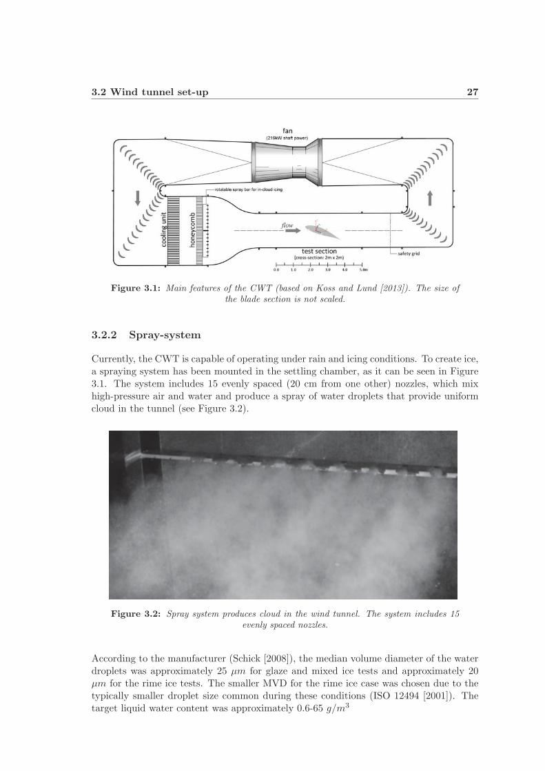
Figure 3.1: Main features of the CWT (based on Koss and Lund [2013]). The size ofthe blade section is not scaled.
3.2.2 Spray-system
Currently, the CWT is capable of operating under rain and icing conditions. To create ice,a spraying system has been mounted in the settling chamber, as it can be seen in Figure3.1. The system includes 15 evenly spaced (20 cm from one other) nozzles, which mixhigh-pressure air and water and produce a spray of water droplets that provide uniformcloud in the tunnel (see Figure 3.2).
Figure 3.2: Spray system produces cloud in the wind tunnel. The system includes 15evenly spaced nozzles.
According to the manufacturer (Schick [2008]), the median volume diameter of the waterdroplets was approximately 25 μm for glaze and mixed ice tests and approximately 20μm for the rime ice tests. The smaller MVD for the rime ice case was chosen due to thetypically smaller droplet size common during these conditions (ISO 12494 [2001]). Thetarget liquid water content was approximately 0.6-65 g/m3
28 Experimental investigation of the effect of ice on wind turbine blades
3.2.3 Airfoil and testing rig
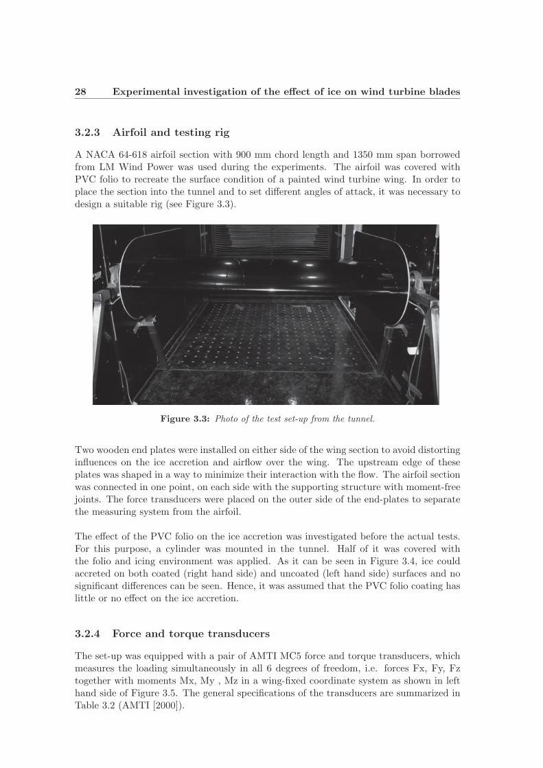
A NACA 64-618 airfoil section with 900 mm chord length and 1350 mm span borrowedfrom LM Wind Power was used during the experiments. The airfoil was covered withPVC folio to recreate the surface condition of a painted wind turbine wing. In order toplace the section into the tunnel and to set different angles of attack, it was necessary todesign a suitable rig (see Figure 3.3).
Figure 3.3: Photo of the test set-up from the tunnel.
Two wooden end plates were installed on either side of the wing section to avoid distortinginfluences on the ice accretion and airflow over the wing. The upstream edge of theseplates was shaped in a way to minimize their interaction with the flow. The airfoil sectionwas connected in one point, on each side with the supporting structure with moment-freejoints. The force transducers were placed on the outer side of the end-plates to separatethe measuring system from the airfoil.
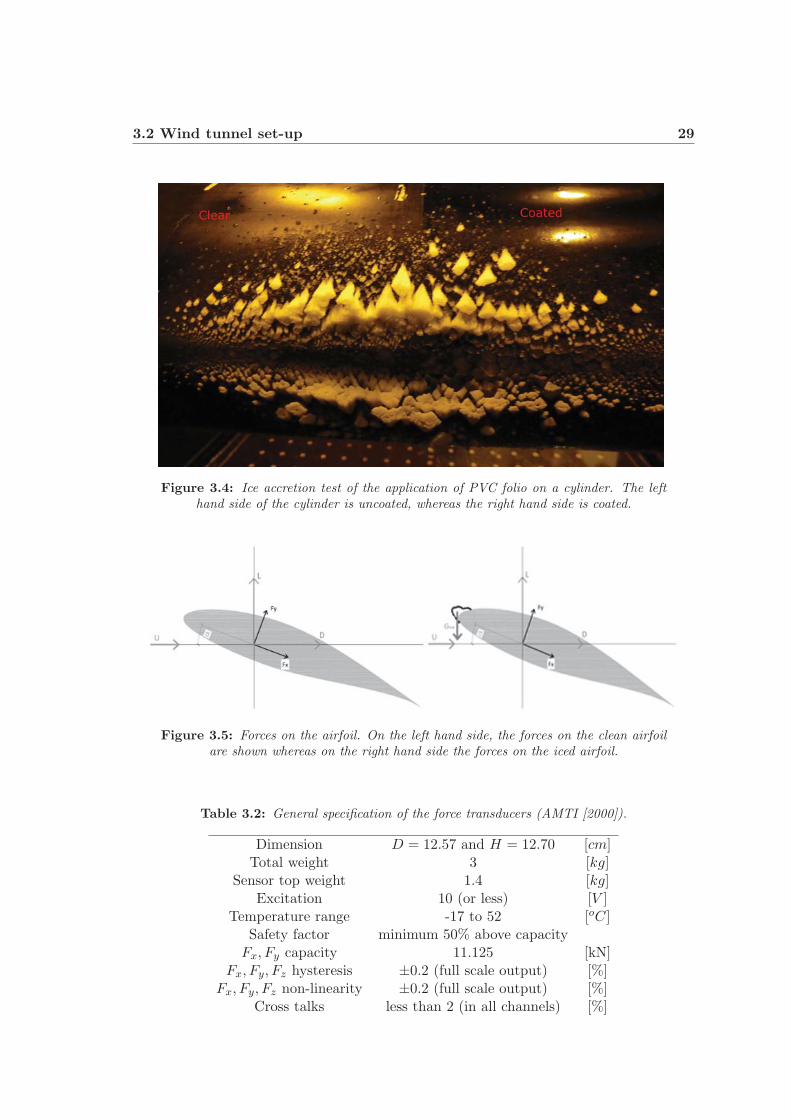
The effect of the PVC folio on the ice accretion was investigated before the actual tests.For this purpose, a cylinder was mounted in the tunnel. Half of it was covered withthe folio and icing environment was applied. As it can be seen in Figure 3.4, ice couldaccreted on both coated (right hand side) and uncoated (left hand side) surfaces and nosignificant differences can be seen. Hence, it was assumed that the PVC folio coating haslittle or no effect on the ice accretion.
3.2.4 Force and torque transducers
The set-up was equipped with a pair of AMTI MC5 force and torque transducers, whichmeasures the loading simultaneously in all 6 degrees of freedom, i.e. forces Fx, Fy, Fztogether with moments Mx, My , Mz in a wing-fixed coordinate system as shown in lefthand side of Figure 3.5. The general specifications of the transducers are summarized inTable 3.2 (AMTI [2000]).
3.2 Wind tunnel set-up 29
Figure 3.4: Ice accretion test of the application of PVC folio on a cylinder. The lefthand side of the cylinder is uncoated, whereas the right hand side is coated.
Figure 3.5: Forces on the airfoil. On the left hand side, the forces on the clean airfoilare shown whereas on the right hand side the forces on the iced airfoil.
Table 3.2: General specification of the force transducers (AMTI [2000]).
Dimension D = 12.57 and H = 12.70 [cm]Total weight 3 [kg]
Sensor top weight 1.4 [kg]Excitation 10 (or less) [V ]
Temperature range -17 to 52 [oC]Safety factor minimum 50% above capacity
Fx, Fy capacity 11.125 [kN]Fx, Fy, Fz hysteresis ±0.2 (full scale output) [%]
Fx, Fy, Fz non-linearity ±0.2 (full scale output) [%]Cross talks less than 2 (in all channels) [%]

30 Experimental investigation of the effect of ice on wind turbine blades
Beside the force transducers, it was necessary to use a power amplifier for each transducerwith relative power supply, a National Instrument analogue input module and a NationalInstrument CompactDAQ Chassis for the measurements in order to read the signal fromthe transducers and the other sensors and transport the data to the computer.
3.2.5 Data calibration
The data registered by the force transducers are in [V] and these values need to beconverted to [N] (and [Nm]) using the following equations (eq.3.1 - 3.2):
Fx[N ] = [Fx[V ]B1,1
GFx+
Fy[V ]B1,2
GFy+ ...+
Mz[V ]B1,6
GFz] ∗ 106
Exc(3.1)
Fy[N ] = [Fx[V ]B2,1
GFx+
Fy[V ]B2,2
GFy+ ...+
Mz[V ]B2,6
GFz] ∗ 106
Exc(3.2)
where B is the force transducer cross talk-matrix and is dependent on the type of theforce transducer. i.e. each transducer has its own cross talk-matrix. Exc is the excitationfactor, which is monitored by the force transducer and GFx, GFy, GFz, GMx, GMy andGMz are the power amplifier’s gain. Each amplifier has its specific gain values too.
The rotational speed of the fans of the wind tunnel is given in revolutions per minute (rpm)as an input parameter. In Table 3.3, some of the velocities are converted into m/s units.The wind speed (U) in the cross-section can be calculated based on the measurements by
Table 3.3: Example of rotational speed conversion from rpm to m/s on aspecific day.
U (rpm) 100 300 500 700 800 1000
U (m/s) 1.78 5.71 9.64 13.57 15.56 19.49
the Pitot tube using the following expressions:
U =
√2� P
ρ(3.3)
Where �P is the pressure difference measured by a Pitot tube and ρ is the air density inkg/m3 (see eq. 3.4).
ρ =Patm ∗ 100
287.05 ∗ (T + 273.15)∗ (1− 0.378pv
Patm ∗ 100) (3.4)
Where Patm is the atmospheric pressure of the day [mb], T is the temperature in thetunnel in [oC] and pv is the actual vapor pressure from the relative humidity (RH) in[Pa].
pv = Es ∗RH (3.5)
Where Es is the vapor pressure [mb], eq.3.6:
Es = c0 ∗ 10c1 ∗ Tc2 + T (3.6)
3.3 Set-up of wind tunnel tests 31
Where c0 = 6.1078, c1 = 7.5 and c2 = 273.3.As it can be seen from these equations, the wind speed conversion from the Pitot tube ishighly dependent on the daily meteorological parameters, which are constantly changing.
3.3 Set-up of wind tunnel tests
Glaze, mixed. and rime ice deposits built up on a NACA 64-618 profile. The aerodynamicforces acting on the blade during ice accretion for different angles of attack (0o, 4o, 7o, 9o,11o) at various air temperature (approximate, mean value of the set temperature: -3 oC,-5 oC, and -8 oC) were measured along with the mass of ice and the final ice shape. Theused temperature range can be described as rather moderate, but due to the limitationof the wind tunnel’s cooling unit, colder temperatures could not be used.
Ice was building up on the surface of the airfoil section at different temperatures, ensuringthe three investigated icing characteristics for each angle of attack. A list of the windtunnel tests and the conditions can be found in Table 3.4. The values are approximated.Two different air speeds were targeted: one applied for the ice accretion and the other onefor force measurements. The temperature values are mean value of the used temperatureduring the tests.
Table 3.4: A summary of the wind tunnel tests and conditions. The two differentvelocities are target values, one during the ice accretion (Accretion) and the other duringthe force measurements (Tests). The temperature values are mean value of the usedtemperature. The LWC parameters are target values. These numbers are approximated.
Test AOA T Ice MVD LWC U (m/s) U (m/s) ta(o) (oC) (μm) (g/m3) Accretion Tests (min)
1 0 -3 glaze 25 0.65 15 15 602 0 -5 mixed 25 0.65 15 15 603 0 -8 rime 20 0.6 10 15 604 4 -3 glaze 25 0.65 15 15 605 4 -5 mixed 25 0.65 15 15 606 4 -8 rime 20 0.6 10 15 607 7 -3 glaze 25 0.65 15 15 608 7 -5 mixed 25 0.65 15 15 609 7 -8 rime 20 0.6 10 15 6010 9 -3 glaze 25 0.65 15 15 6011 9 -5 mixed 25 0.65 15 15 6012 9 -8 rime 20 0.6 10 15 6113 11 -3 glaze 25 0.65 15 15 6214 11 -5 mixed 25 0.65 15 15 6315 11 -8 rime 20 0.6 10 15 64
The tests were performed by first setting the required wind speed and temperature in thetest section. Water spray, providing in-cloud environment was then initiated. The airspeed was set to 15 m/s (corresponding to Reynolds number, Re� 1E6) for glaze andmixed ice and to 10 m/s (corresponding to Re � 0.6E6) for rime ice accretion and the
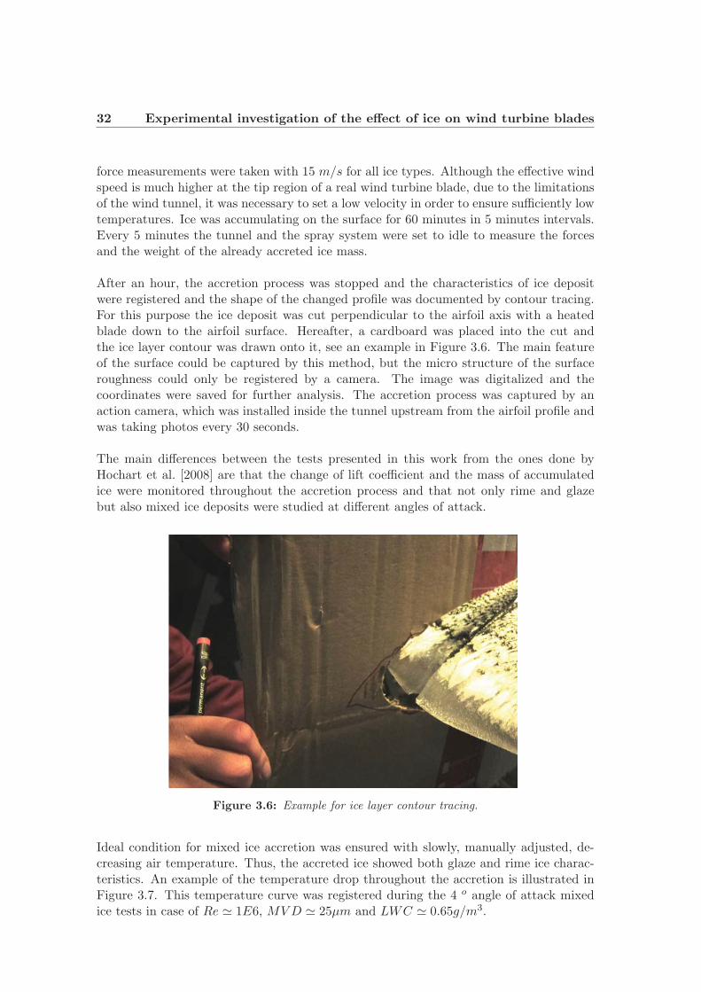
32 Experimental investigation of the effect of ice on wind turbine blades
force measurements were taken with 15 m/s for all ice types. Although the effective windspeed is much higher at the tip region of a real wind turbine blade, due to the limitationsof the wind tunnel, it was necessary to set a low velocity in order to ensure sufficiently lowtemperatures. Ice was accumulating on the surface for 60 minutes in 5 minutes intervals.Every 5 minutes the tunnel and the spray system were set to idle to measure the forcesand the weight of the already accreted ice mass.
After an hour, the accretion process was stopped and the characteristics of ice depositwere registered and the shape of the changed profile was documented by contour tracing.For this purpose the ice deposit was cut perpendicular to the airfoil axis with a heatedblade down to the airfoil surface. Hereafter, a cardboard was placed into the cut andthe ice layer contour was drawn onto it, see an example in Figure 3.6. The main featureof the surface could be captured by this method, but the micro structure of the surfaceroughness could only be registered by a camera. The image was digitalized and thecoordinates were saved for further analysis. The accretion process was captured by anaction camera, which was installed inside the tunnel upstream from the airfoil profile andwas taking photos every 30 seconds.
The main differences between the tests presented in this work from the ones done byHochart et al. [2008] are that the change of lift coefficient and the mass of accumulatedice were monitored throughout the accretion process and that not only rime and glazebut also mixed ice deposits were studied at different angles of attack.
Figure 3.6: Example for ice layer contour tracing.
Ideal condition for mixed ice accretion was ensured with slowly, manually adjusted, de-creasing air temperature. Thus, the accreted ice showed both glaze and rime ice charac-teristics. An example of the temperature drop throughout the accretion is illustrated inFigure 3.7. This temperature curve was registered during the 4 o angle of attack mixedice tests in case of Re � 1E6, MVD � 25μm and LWC � 0.65g/m3.
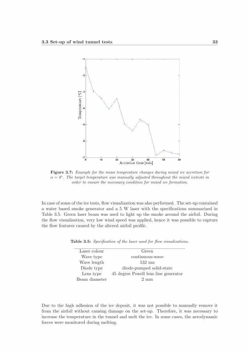
3.3 Set-up of wind tunnel tests 33
Figure 3.7: Example for the mean temperature changes during mixed ice accretion forα = 4o. The target temperature was manually adjusted throughout the mixed icetests in
order to ensure the necessary condition for mixed ice formation.
In case of some of the ice tests, flow visualization was also performed. The set-up containeda water based smoke generator and a 5 W laser with the specifications summarized inTable 3.5. Green laser beam was used to light up the smoke around the airfoil. Duringthe flow visualisation, very low wind speed was applied, hence it was possible to capturethe flow features caused by the altered airfoil profile.
Table 3.5: Specification of the laser used for flow visualizations.
Laser colour GreenWave type continuous-waveWave length 532 nmDiode type diode-pumped solid-stateLens type 45 degree Powell lens line generator
Beam diameter 2 mm
Due to the high adhesion of the ice deposit, it was not possible to manually remove itfrom the airfoil without causing damage on the set-up. Therefore, it was necessary toincrease the temperature in the tunnel and melt the ice. In some cases, the aerodynamicforces were monitored during melting.

34 Experimental investigation of the effect of ice on wind turbine blades
3.4 Wind tunnel correction
The confined flow in the wind tunnel alters the flow field around the airfoil compared tofull-scale and hence affects the measured aerodynamic forces on the wing section. Themeasured forces were corrected for both, lift interference and blockage interference. Liftinterference is caused by the changes of the stream direction and stream curvature, andthe blockage interference is the result of the changes in stream velocity and longitudinalpressure gradient. These two interferences are independent of each other (ESDU 76028[1976]). The tunnel correction was performed by following ESDU 76028 Lift-interferenceand blockage corrections for two-dimensional subsonic flow in ventilated and closed wind-tunnels methodology.
These equations were derived with the linearised potential flow theory (detailed in ESDU76028) and are valid for subsonic flows. The incremental correction of lift coefficient(�CL) due to lift interference can be calculated by integrating the residual loading cor-rection along the airfoil chord (c):
�CL = −π
2
( c
h
)2 δ1β2
CL (3.7)
δ1 represents the effect of changes in streamline curvature, c is the chord length and
h is the height of the wind tunnel. In case of closed wind tunnels, δ1=π
24. β is the
Prandtl-Glauert compressibility parameter, which depends on the Mach number (M∞),
β =(1−M2∞
)1/2. The drag coefficient correction (�CD) can be done as followed:
�CDB = −−2A2eK
cβ4h3− CDΩsεsc (3.8)
�CDR = − c
hδ0C
2L (3.9)
However, K = 0 and δ0= 0 for closed wind tunnels, which makes these equations evensimpler. The blockage is a combination of the model and the wake, therefore both has tobe added to the blockage factor, εB.
εB = Ωsεsc +Ωwεwc (3.10)
Ωs and Ωw are the blockage factor rations and have unit magnitude for the closed windtunnels.
εsc =φAe
6β3h2(3.11)
εwc =1
4
( c
h
) CD
β2(3.12)
Ae is an equivalent area for the airfoil section and CD is the drag coefficient. The aero-dynamic coefficients from the wind tunnel measurements need to be corrected to free-airvalues by the ratio of the corrected to uncorrected kinetic pressure, G.
G =1
1 + (1−M2∞)εB(3.13)
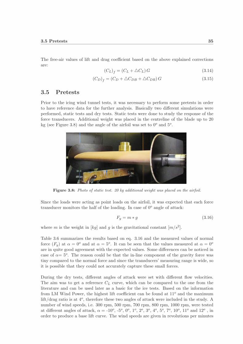
3.5 Pretests 35
The free-air values of lift and drag coefficient based on the above explained correctionsare:
(CL)f = (CL +�CL)G (3.14)
(CD)f = (CD +�CDB +�CDR)G (3.15)
3.5 Pretests
Prior to the icing wind tunnel tests, it was necessary to perform some pretests in orderto have reference data for the further analysis. Basically two different simulations wereperformed, static tests and dry tests. Static tests were done to study the response of theforce transducers. Additional weight was placed in the centreline of the blade up to 20kg (see Figure 3.8) and the angle of the airfoil was set to 0o and 5o.
Figure 3.8: Photo of static test. 20 kg additional weight was placed on the airfoil.
Since the loads were acting as point loads on the airfoil, it was expected that each forcetransducer monitors the half of the loading. In case of 0o angle of attack:
Fy = m ∗ g (3.16)
where m is the weight in [kg] and g is the gravitational constant [m/s2].
Table 3.6 summarizes the results based on eq. 3.16 and the measured values of normalforce (Fy) at α = 0o and at α = 5o. It can be seen that the values measured at α = 0o
are in quite good agreement with the expected values. Some differences can be noticed incase of α= 5o. The reason could be that the in-line component of the gravity force wastiny compared to the normal force and since the transducers’ measuring range is wide, soit is possible that they could not accurately capture these small forces.
During the dry tests, different angles of attack were set with different flow velocities.The aim was to get a reference CL curve, which can be compared to the one from theliterature and can be used later as a basic for the ice tests. Based on the informationfrom LM Wind Power, the highest lift coefficient can be found at 11o and the maximumlift/drag ratio is at 4o, therefore these two angles of attack were included in the study. Anumber of wind speeds, i.e. 300 rpm, 500 rpm, 700 rpm, 800 rpm, 1000 rpm, were testedat different angles of attack, α = -10o, -5o, 0o, 1o, 2o, 3o, 4o, 5o, 7o, 10o, 11o and 12o , inorder to produce a base lift curve. The wind speeds are given in revolutions per minutes
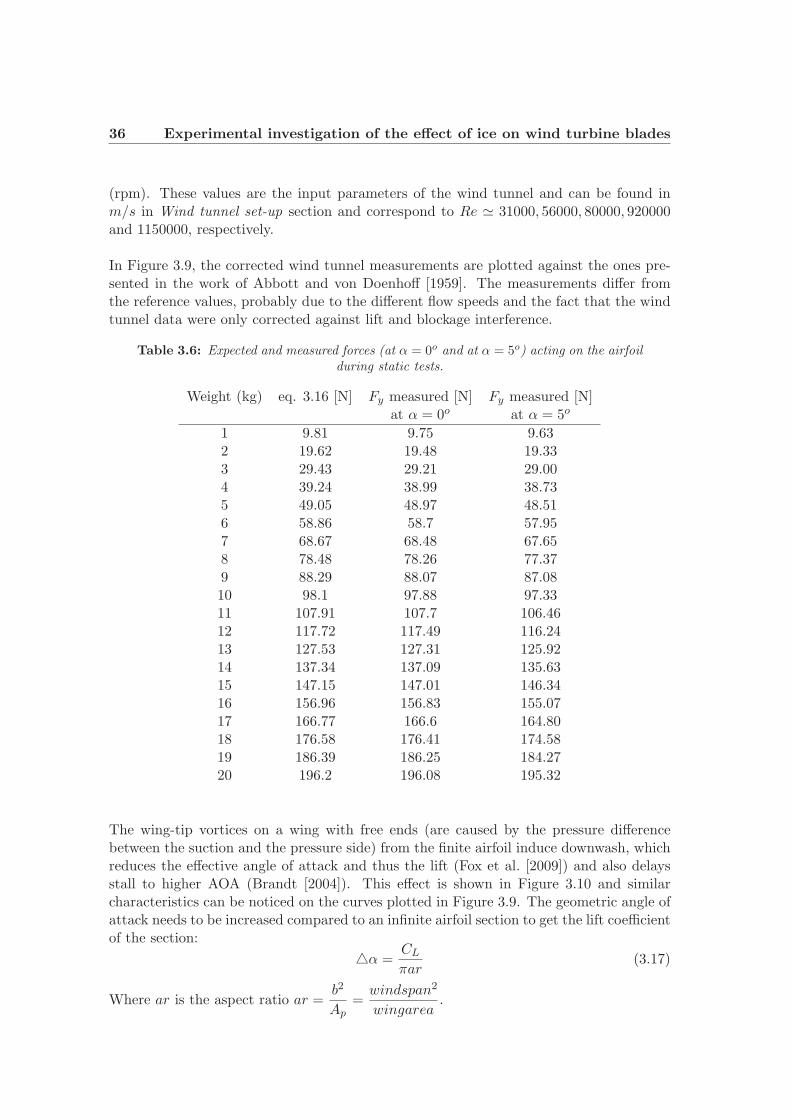
36 Experimental investigation of the effect of ice on wind turbine blades
(rpm). These values are the input parameters of the wind tunnel and can be found inm/s in Wind tunnel set-up section and correspond to Re � 31000, 56000, 80000, 920000and 1150000, respectively.
In Figure 3.9, the corrected wind tunnel measurements are plotted against the ones pre-sented in the work of Abbott and von Doenhoff [1959]. The measurements differ fromthe reference values, probably due to the different flow speeds and the fact that the windtunnel data were only corrected against lift and blockage interference.
Table 3.6: Expected and measured forces (at α = 0o and at α = 5o) acting on the airfoilduring static tests.
Weight (kg) eq. 3.16 [N] Fy measured [N] Fy measured [N]at α = 0o at α = 5o
1 9.81 9.75 9.632 19.62 19.48 19.333 29.43 29.21 29.004 39.24 38.99 38.735 49.05 48.97 48.516 58.86 58.7 57.957 68.67 68.48 67.658 78.48 78.26 77.379 88.29 88.07 87.0810 98.1 97.88 97.3311 107.91 107.7 106.4612 117.72 117.49 116.2413 127.53 127.31 125.9214 137.34 137.09 135.6315 147.15 147.01 146.3416 156.96 156.83 155.0717 166.77 166.6 164.8018 176.58 176.41 174.5819 186.39 186.25 184.2720 196.2 196.08 195.32
The wing-tip vortices on a wing with free ends (are caused by the pressure differencebetween the suction and the pressure side) from the finite airfoil induce downwash, whichreduces the effective angle of attack and thus the lift (Fox et al. [2009]) and also delaysstall to higher AOA (Brandt [2004]). This effect is shown in Figure 3.10 and similarcharacteristics can be noticed on the curves plotted in Figure 3.9. The geometric angle ofattack needs to be increased compared to an infinite airfoil section to get the lift coefficientof the section:
�α =CL
πar(3.17)
Where ar is the aspect ratio ar =b2
Ap=
windspan2
wingarea.
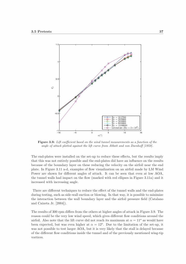
3.5 Pretests 37
Figure 3.9: Lift coefficient based on the wind tunnel measurements as a function of theangle of attack plotted against the lift curve from Abbott and von Doenhoff [1959].
The end-plates were installed on the set-up to reduce these effects, but the results implythat this was not entirely possible and the end-plates did have an influence on the resultsbecause of the boundary layer on these reducing the velocity on the airfoil near the endplate. In Figure 3.11 a-d, examples of flow visualization on an airfoil made by LM WindPower are shown for different angles of attack. It can be seen that even at low AOA,the tunnel walls had impact on the flow (marked with red ellipses in Figure 3.11a) and itincreased with increasing angle.
There are different techniques to reduce the effect of the tunnel walls and the end-platesduring testing, such as side-wall suction or blowing. In that way, it is possible to minimizethe interaction between the wall boundary layer and the airfoil pressure field (Catalanoand Caixeta Jr. [2004]).
The results of 300 rpm differs from the others at higher angles of attack in Figure 3.9. Thereason could be the very low wind speed, which gives different flow conditions around theairfoil. Also note that the lift curve did not reach its maximum at α = 11o as would havebeen expected, but was even higher at α = 12o. Due to the limitation of the set-up, itwas not possible to test larger AOA, but it is very likely that the stall is delayed becauseof the different flow conditions inside the tunnel and of the previously mentioned wing-tipvortices.
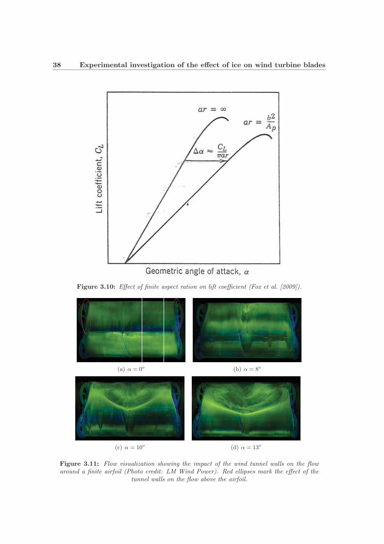
38 Experimental investigation of the effect of ice on wind turbine blades
Figure 3.10: Effect of finite aspect ration on lift coefficient (Fox et al. [2009]).
(a) α = 0o (b) α = 8o
(c) α = 10o (d) α = 13o
Figure 3.11: Flow visualization showing the impact of the wind tunnel walls on the flowaround a finite airfoil (Photo credit: LM Wind Power). Red ellipses mark the effect of the
tunnel walls on the flow above the airfoil.
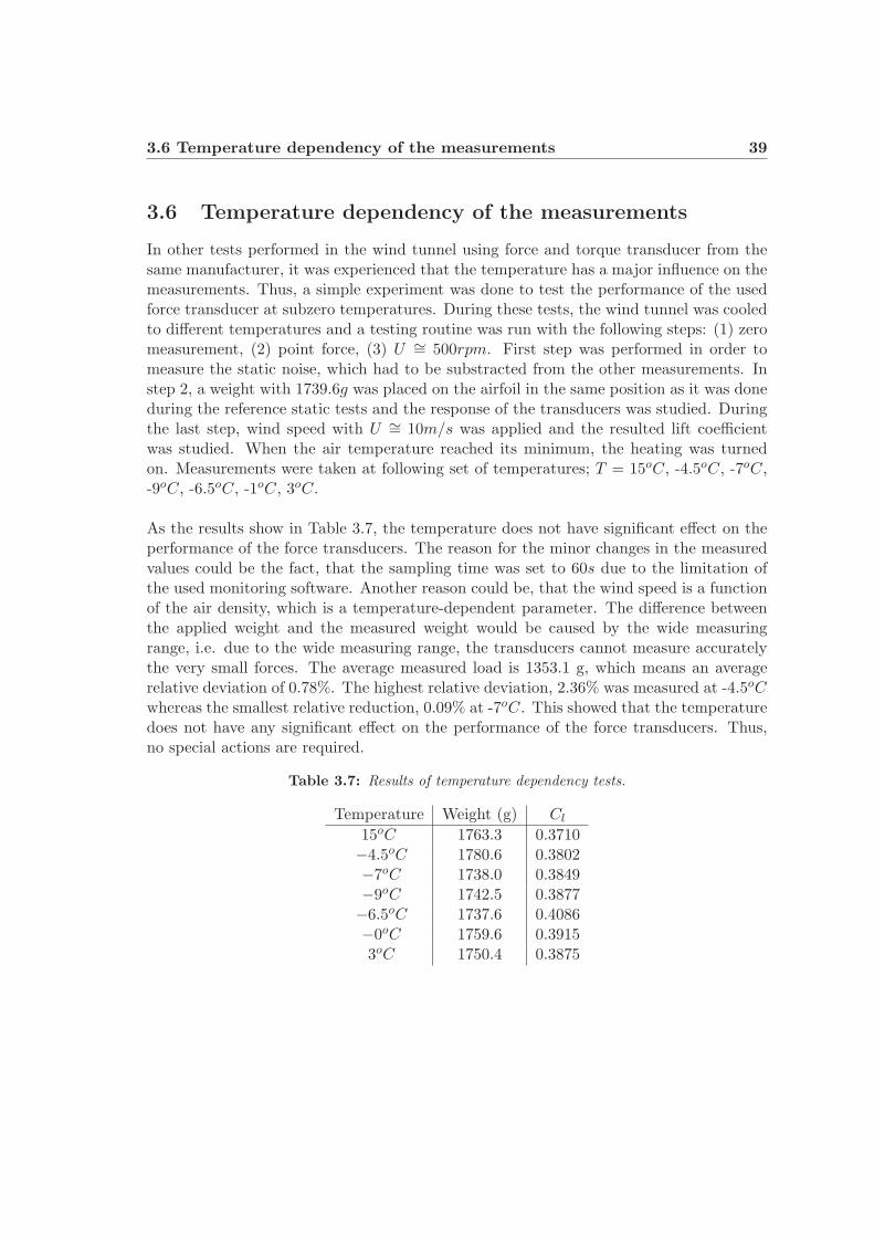
3.6 Temperature dependency of the measurements 39
3.6 Temperature dependency of the measurements
In other tests performed in the wind tunnel using force and torque transducer from thesame manufacturer, it was experienced that the temperature has a major influence on themeasurements. Thus, a simple experiment was done to test the performance of the usedforce transducer at subzero temperatures. During these tests, the wind tunnel was cooledto different temperatures and a testing routine was run with the following steps: (1) zeromeasurement, (2) point force, (3) U ∼= 500rpm. First step was performed in order tomeasure the static noise, which had to be substracted from the other measurements. Instep 2, a weight with 1739.6g was placed on the airfoil in the same position as it was doneduring the reference static tests and the response of the transducers was studied. Duringthe last step, wind speed with U ∼= 10m/s was applied and the resulted lift coefficientwas studied. When the air temperature reached its minimum, the heating was turnedon. Measurements were taken at following set of temperatures; T = 15oC, -4.5oC, -7oC,-9oC, -6.5oC, -1oC, 3oC.
As the results show in Table 3.7, the temperature does not have significant effect on theperformance of the force transducers. The reason for the minor changes in the measuredvalues could be the fact, that the sampling time was set to 60s due to the limitation ofthe used monitoring software. Another reason could be, that the wind speed is a functionof the air density, which is a temperature-dependent parameter. The difference betweenthe applied weight and the measured weight would be caused by the wide measuringrange, i.e. due to the wide measuring range, the transducers cannot measure accuratelythe very small forces. The average measured load is 1353.1 g, which means an averagerelative deviation of 0.78%. The highest relative deviation, 2.36% was measured at -4.5oCwhereas the smallest relative reduction, 0.09% at -7oC. This showed that the temperaturedoes not have any significant effect on the performance of the force transducers. Thus,no special actions are required.
Table 3.7: Results of temperature dependency tests.
Temperature Weight (g) Cl
15oC 1763.3 0.3710−4.5oC 1780.6 0.3802−7oC 1738.0 0.3849−9oC 1742.5 0.3877−6.5oC 1737.6 0.4086−0oC 1759.6 0.39153oC 1750.4 0.3875
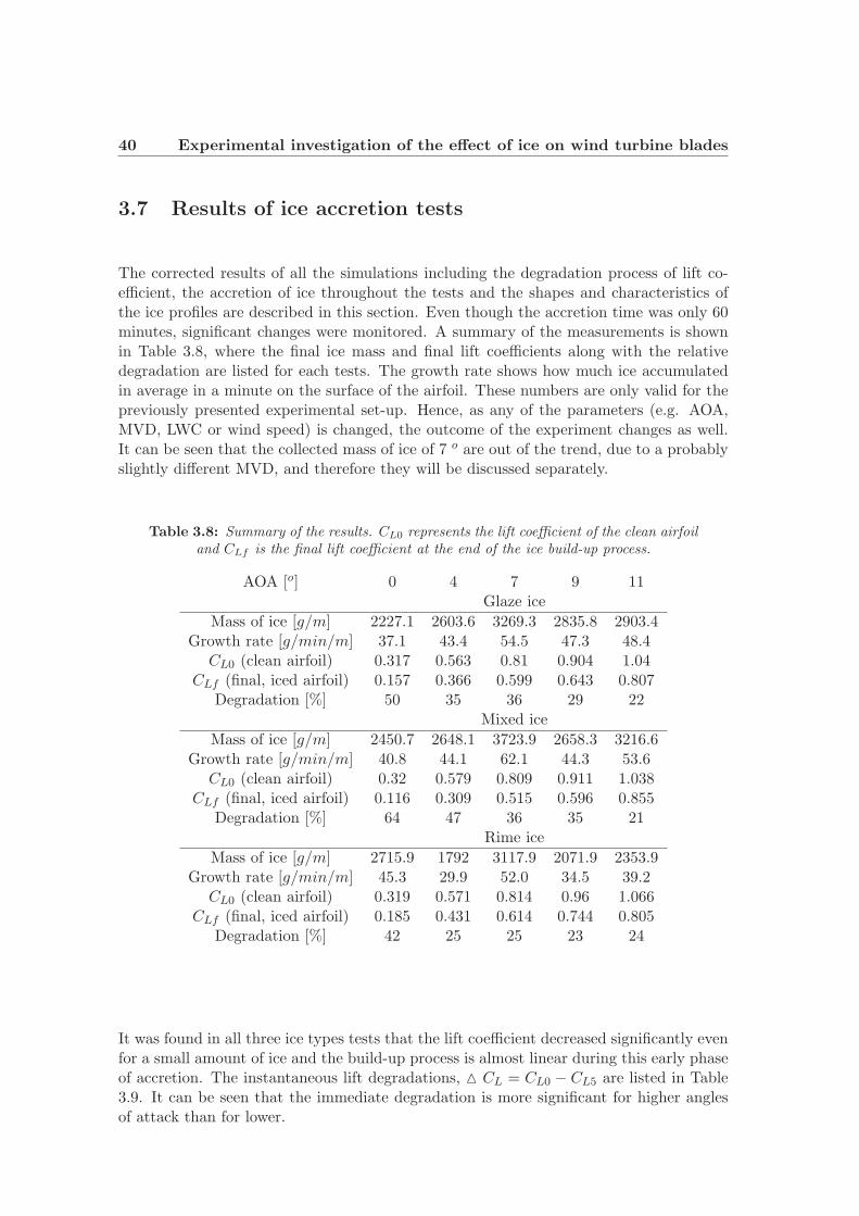
40 Experimental investigation of the effect of ice on wind turbine blades
3.7 Results of ice accretion tests
The corrected results of all the simulations including the degradation process of lift co-efficient, the accretion of ice throughout the tests and the shapes and characteristics ofthe ice profiles are described in this section. Even though the accretion time was only 60minutes, significant changes were monitored. A summary of the measurements is shownin Table 3.8, where the final ice mass and final lift coefficients along with the relativedegradation are listed for each tests. The growth rate shows how much ice accumulatedin average in a minute on the surface of the airfoil. These numbers are only valid for thepreviously presented experimental set-up. Hence, as any of the parameters (e.g. AOA,MVD, LWC or wind speed) is changed, the outcome of the experiment changes as well.It can be seen that the collected mass of ice of 7 o are out of the trend, due to a probablyslightly different MVD, and therefore they will be discussed separately.
Table 3.8: Summary of the results. CL0 represents the lift coefficient of the clean airfoiland CLf is the final lift coefficient at the end of the ice build-up process.
AOA [o] 0 4 7 9 11Glaze ice
Mass of ice [g/m] 2227.1 2603.6 3269.3 2835.8 2903.4Growth rate [g/min/m] 37.1 43.4 54.5 47.3 48.4
CL0 (clean airfoil) 0.317 0.563 0.81 0.904 1.04CLf (final, iced airfoil) 0.157 0.366 0.599 0.643 0.807
Degradation [%] 50 35 36 29 22Mixed ice
Mass of ice [g/m] 2450.7 2648.1 3723.9 2658.3 3216.6Growth rate [g/min/m] 40.8 44.1 62.1 44.3 53.6
CL0 (clean airfoil) 0.32 0.579 0.809 0.911 1.038CLf (final, iced airfoil) 0.116 0.309 0.515 0.596 0.855
Degradation [%] 64 47 36 35 21Rime ice
Mass of ice [g/m] 2715.9 1792 3117.9 2071.9 2353.9Growth rate [g/min/m] 45.3 29.9 52.0 34.5 39.2
CL0 (clean airfoil) 0.319 0.571 0.814 0.96 1.066CLf (final, iced airfoil) 0.185 0.431 0.614 0.744 0.805
Degradation [%] 42 25 25 23 24
It was found in all three ice types tests that the lift coefficient decreased significantly evenfor a small amount of ice and the build-up process is almost linear during this early phaseof accretion. The instantaneous lift degradations, � CL = CL0 − CL5 are listed in Table3.9. It can be seen that the immediate degradation is more significant for higher anglesof attack than for lower.
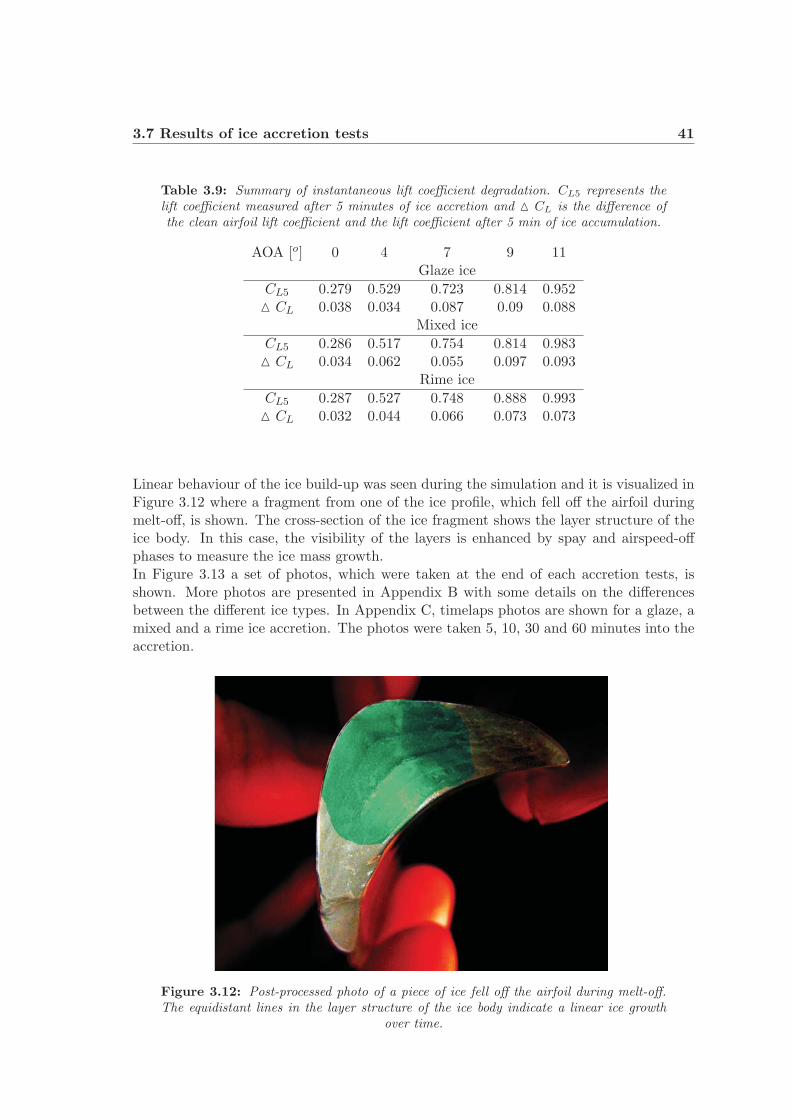
3.7 Results of ice accretion tests 41
Table 3.9: Summary of instantaneous lift coefficient degradation. CL5 represents thelift coefficient measured after 5 minutes of ice accretion and � CL is the difference ofthe clean airfoil lift coefficient and the lift coefficient after 5 min of ice accumulation.
AOA [o] 0 4 7 9 11Glaze ice
CL5 0.279 0.529 0.723 0.814 0.952� CL 0.038 0.034 0.087 0.09 0.088
Mixed ice
CL5 0.286 0.517 0.754 0.814 0.983� CL 0.034 0.062 0.055 0.097 0.093
Rime ice
CL5 0.287 0.527 0.748 0.888 0.993� CL 0.032 0.044 0.066 0.073 0.073
Linear behaviour of the ice build-up was seen during the simulation and it is visualized inFigure 3.12 where a fragment from one of the ice profile, which fell off the airfoil duringmelt-off, is shown. The cross-section of the ice fragment shows the layer structure of theice body. In this case, the visibility of the layers is enhanced by spay and airspeed-offphases to measure the ice mass growth.In Figure 3.13 a set of photos, which were taken at the end of each accretion tests, isshown. More photos are presented in Appendix B with some details on the differencesbetween the different ice types. In Appendix C, timelaps photos are shown for a glaze, amixed and a rime ice accretion. The photos were taken 5, 10, 30 and 60 minutes into theaccretion.
Figure 3.12: Post-processed photo of a piece of ice fell off the airfoil during melt-off.The equidistant lines in the layer structure of the ice body indicate a linear ice growth
over time.
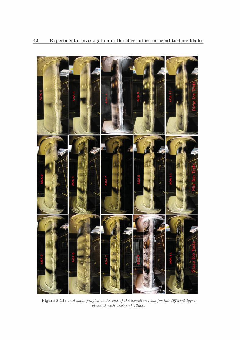
42 Experimental investigation of the effect of ice on wind turbine blades
Figure 3.13: Iced blade profiles at the end of the accretion tests for the different typesof ice at each angles of attack.
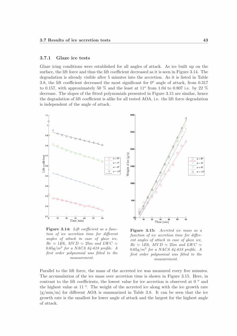
3.7 Results of ice accretion tests 43
3.7.1 Glaze ice tests
Glaze icing conditions were established for all angles of attack. As ice built up on thesurface, the lift force and thus the lift coefficient decreased as it is seen in Figure 3.14. Thedegradation is already visible after 5 minutes into the accretion. As it is listed in Table3.8, the lift coefficient decreased the most significant for 0o angle of attack, from 0.317to 0.157, with approximately 50 % and the least at 11o from 1.04 to 0.807 i.e. by 22 %decrease. The slopes of the fitted polynomials presented in Figure 3.15 are similar, hencethe degradation of lift coefficient is alike for all tested AOA, i.e. the lift force degradationis independent of the angle of attack.
Figure 3.14: Lift coefficient as a func-tion of ice accretion time for differentangles of attack in case of glaze ice,Re � 1E6, MVD � 25m and LWC �0.65g/m3 for a NACA 64-618 profile. Afirst order polynomial was fitted to the
measurement.
Figure 3.15: Accreted ice mass as afunction of ice accretion time for differ-ent angles of attack in case of glaze ice,Re � 1E6, MVD � 25m and LWC �0.65g/m3 for a NACA 64-618 profile. Afirst order polynomial was fitted to the
measurement.
Parallel to the lift force, the mass of the accreted ice was measured every five minutes.The accumulation of the ice mass over accretion time is shown in Figure 3.15. Here, incontrast to the lift coefficients, the lowest value for ice accretion is observed at 0 o andthe highest value at 11 o. The weight of the accreted ice along with the ice growth rate(g/min/m) for different AOA is summarized in Table 3.8. It can be seen that the icegrowth rate is the smallest for lower angle of attack and the largest for the highest angleof attack.
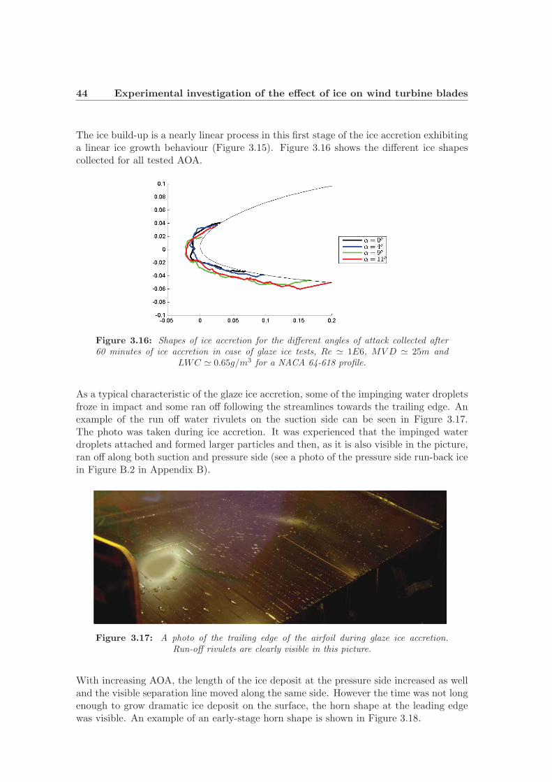
44 Experimental investigation of the effect of ice on wind turbine blades
The ice build-up is a nearly linear process in this first stage of the ice accretion exhibitinga linear ice growth behaviour (Figure 3.15). Figure 3.16 shows the different ice shapescollected for all tested AOA.
Figure 3.16: Shapes of ice accretion for the different angles of attack collected after60 minutes of ice accretion in case of glaze ice tests, Re � 1E6, MVD � 25m and
LWC � 0.65g/m3 for a NACA 64-618 profile.
As a typical characteristic of the glaze ice accretion, some of the impinging water dropletsfroze in impact and some ran off following the streamlines towards the trailing edge. Anexample of the run off water rivulets on the suction side can be seen in Figure 3.17.The photo was taken during ice accretion. It was experienced that the impinged waterdroplets attached and formed larger particles and then, as it is also visible in the picture,ran off along both suction and pressure side (see a photo of the pressure side run-back icein Figure B.2 in Appendix B).
Figure 3.17: A photo of the trailing edge of the airfoil during glaze ice accretion.Run-off rivulets are clearly visible in this picture.
With increasing AOA, the length of the ice deposit at the pressure side increased as welland the visible separation line moved along the same side. However the time was not longenough to grow dramatic ice deposit on the surface, the horn shape at the leading edgewas visible. An example of an early-stage horn shape is shown in Figure 3.18.

3.7 Results of ice accretion tests 45
Figure 3.18: A close-up photo of an early-stage horn ice shape shows a clear separationline between the suction and pressure side. The photo was taken after 60 minutes ofglaze ice accretion in case of 0 o angle of attack and Re � 1E6, MVD � 25m and
LWC � 0.65g/m3 for a NACA 64-618 profile.
3.7.2 Mixed ice tests
The accreted ice showed both glaze and rime ice characteristics. The lift coefficient asa function of the ice accretion time is shown in Figure 3.19 and the final coefficients aresummarized in Table 3.8. As for the glaze ice test results, the process is linear, and alinear curve fitting was applied.
The degradation of the lift coefficient under mixed ice accretion is similar to the changesunder glaze ice accretion. The most significant reduction was found at 0o angle of attack,where the lift coefficient decreased with 64 % from 0.320 to 0.116 after 60 minutes of iceaccretion and the least significant at the highest angle, 11o from 1.038 to 0.855, whichcorresponds to a reduction of approximately 21 %. In Figure 3.20, the accreted ice massis presented as a function of time. The build-up process is practically linear as it wasseen also for the glaze ice tests. As it is given in Table 3.8, the smallest growth rate, 40.8g/min/m was found at 0 o angle of attack and largest, 53.6 g/min/m at 11o.
With increasing angle of attack, the amount of ice build-up on the surface was increasingas well. The sampled ice profiles are plotted in Figure 3.21. The stagnation point is quitevisual due to the thin nose-like peak appearing at the leading edge. As it can be seen,the peak moved towards the pressure side as the angle of attack increased.
In Figure 3.22, an example of a typical mixed ice profile is shown. The photo was takenfollowing the location of the stagnation point at the leading edge of the iced profile setat 4o. The sample shows characteristics of mixed ice. Close to the center, the ice depositis more glassy and smooth whereas in the outer areas, the typical milky feathers of rimeice are visible. See a close-up shot of the feathers in Figure B.1 a in Appendix B.
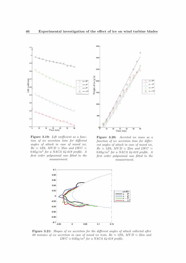
46 Experimental investigation of the effect of ice on wind turbine blades
Figure 3.19: Lift coefficient as a func-tion of ice accretion time for differentangles of attack in case of mixed ice,Re � 1E6, MVD � 25m and LWC �0.65g/m3 for a NACA 64-618 profile. Afirst order polynomial was fitted to the
measurement.
Figure 3.20: Accreted ice mass as afunction of ice accretion time for differ-ent angles of attack in case of mixed ice,Re � 1E6, MVD � 25m and LWC �0.65g/m3 for a NACA 64-618 profile. Afirst order polynomial was fitted to the
measurement.
Figure 3.21: Shapes of ice accretion for the different angles of attack collected after60 minutes of ice accretion in case of mixed ice tests, Re � 1E6, MVD � 25m and
LWC � 0.65g/m3 for a NACA 64-618 profile.
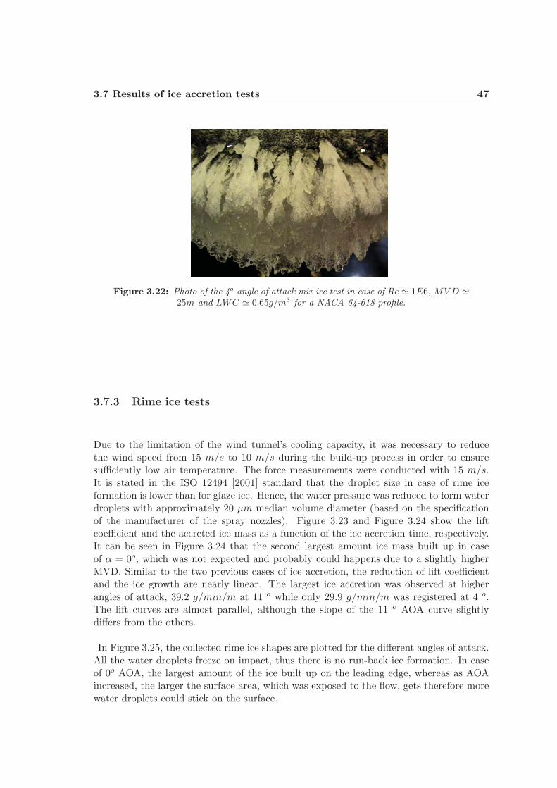
3.7 Results of ice accretion tests 47
Figure 3.22: Photo of the 4o angle of attack mix ice test in case of Re � 1E6, MVD �25m and LWC � 0.65g/m3 for a NACA 64-618 profile.
3.7.3 Rime ice tests
Due to the limitation of the wind tunnel’s cooling capacity, it was necessary to reducethe wind speed from 15 m/s to 10 m/s during the build-up process in order to ensuresufficiently low air temperature. The force measurements were conducted with 15 m/s.It is stated in the ISO 12494 [2001] standard that the droplet size in case of rime iceformation is lower than for glaze ice. Hence, the water pressure was reduced to form waterdroplets with approximately 20 μm median volume diameter (based on the specificationof the manufacturer of the spray nozzles). Figure 3.23 and Figure 3.24 show the liftcoefficient and the accreted ice mass as a function of the ice accretion time, respectively.It can be seen in Figure 3.24 that the second largest amount ice mass built up in caseof α = 0o, which was not expected and probably could happens due to a slightly higherMVD. Similar to the two previous cases of ice accretion, the reduction of lift coefficientand the ice growth are nearly linear. The largest ice accretion was observed at higherangles of attack, 39.2 g/min/m at 11 o while only 29.9 g/min/m was registered at 4 o.The lift curves are almost parallel, although the slope of the 11 o AOA curve slightlydiffers from the others.
In Figure 3.25, the collected rime ice shapes are plotted for the different angles of attack.All the water droplets freeze on impact, thus there is no run-back ice formation. In caseof 0o AOA, the largest amount of the ice built up on the leading edge, whereas as AOAincreased, the larger the surface area, which was exposed to the flow, gets therefore morewater droplets could stick on the surface.

48 Experimental investigation of the effect of ice on wind turbine blades
Figure 3.23: Lift coefficient as a func-tion of ice accretion time for differentangles of attack in case of rime ice ac-creted for Re � 6E5 MVD � 20m andLWC � 0.6g/m3 on a NACA 64-618 pro-file. A first order polynomial was fitted to
the measurement.
Figure 3.24: Accreted ice mass as afunction of ice accretion time for differ-ent angles of attack in case of rime icefor Re � 6E5 MVD � 20m and LWC �0.6g/m3 on a NACA 64-618 profile. Afirst order polynomial was fitted to the
measurement.
Figure 3.25: Shapes of ice accretion for the different angles of attack collected after60 minutes of ice accretion in case of rime ice tests for Re � 6E5 MVD � 20m and
LWC � 0.6g/m3 on a NACA 64-618 profile.
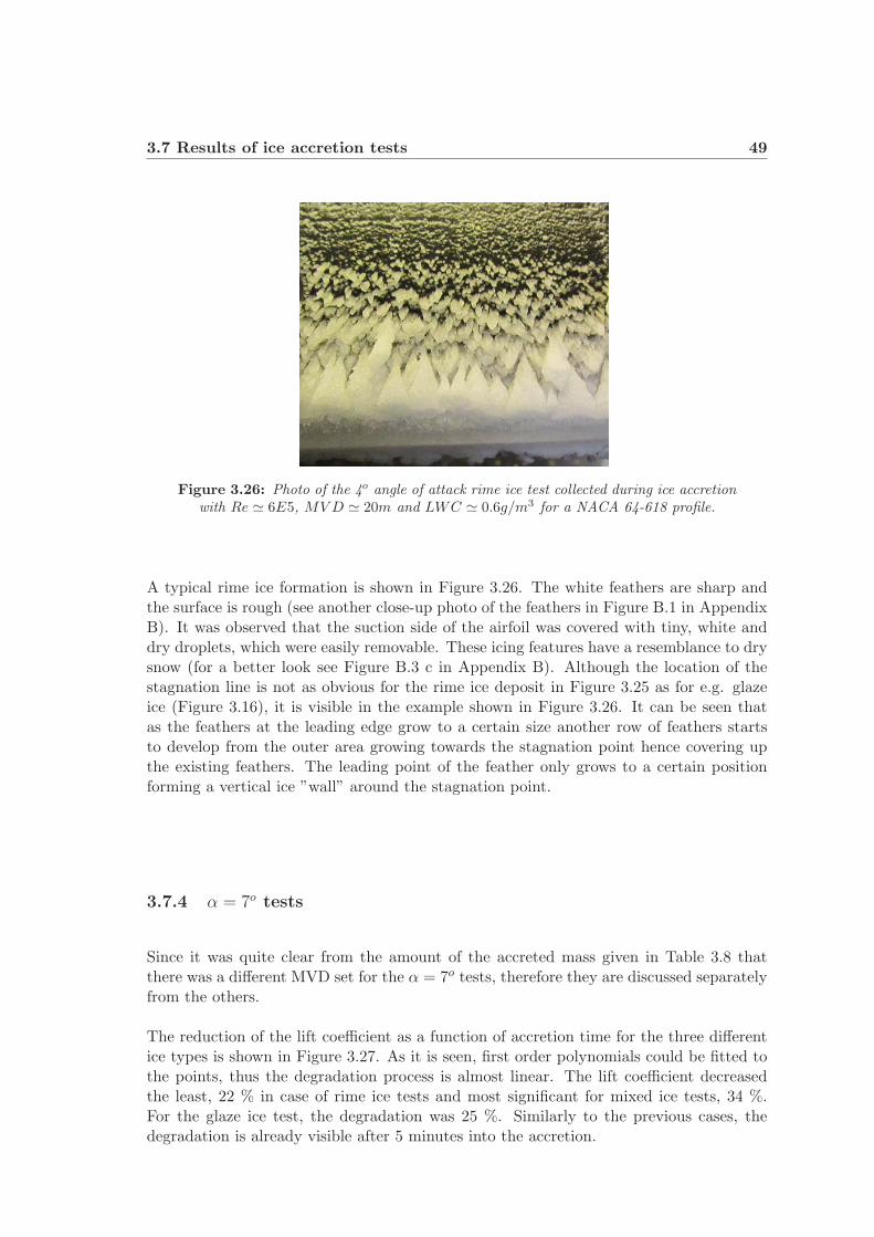
3.7 Results of ice accretion tests 49
Figure 3.26: Photo of the 4o angle of attack rime ice test collected during ice accretionwith Re � 6E5, MVD � 20m and LWC � 0.6g/m3 for a NACA 64-618 profile.
A typical rime ice formation is shown in Figure 3.26. The white feathers are sharp andthe surface is rough (see another close-up photo of the feathers in Figure B.1 in AppendixB). It was observed that the suction side of the airfoil was covered with tiny, white anddry droplets, which were easily removable. These icing features have a resemblance to drysnow (for a better look see Figure B.3 c in Appendix B). Although the location of thestagnation line is not as obvious for the rime ice deposit in Figure 3.25 as for e.g. glazeice (Figure 3.16), it is visible in the example shown in Figure 3.26. It can be seen thatas the feathers at the leading edge grow to a certain size another row of feathers startsto develop from the outer area growing towards the stagnation point hence covering upthe existing feathers. The leading point of the feather only grows to a certain positionforming a vertical ice ”wall” around the stagnation point.
3.7.4 α = 7o tests
Since it was quite clear from the amount of the accreted mass given in Table 3.8 thatthere was a different MVD set for the α = 7o tests, therefore they are discussed separatelyfrom the others.
The reduction of the lift coefficient as a function of accretion time for the three differentice types is shown in Figure 3.27. As it is seen, first order polynomials could be fitted tothe points, thus the degradation process is almost linear. The lift coefficient decreasedthe least, 22 % in case of rime ice tests and most significant for mixed ice tests, 34 %.For the glaze ice test, the degradation was 25 %. Similarly to the previous cases, thedegradation is already visible after 5 minutes into the accretion.
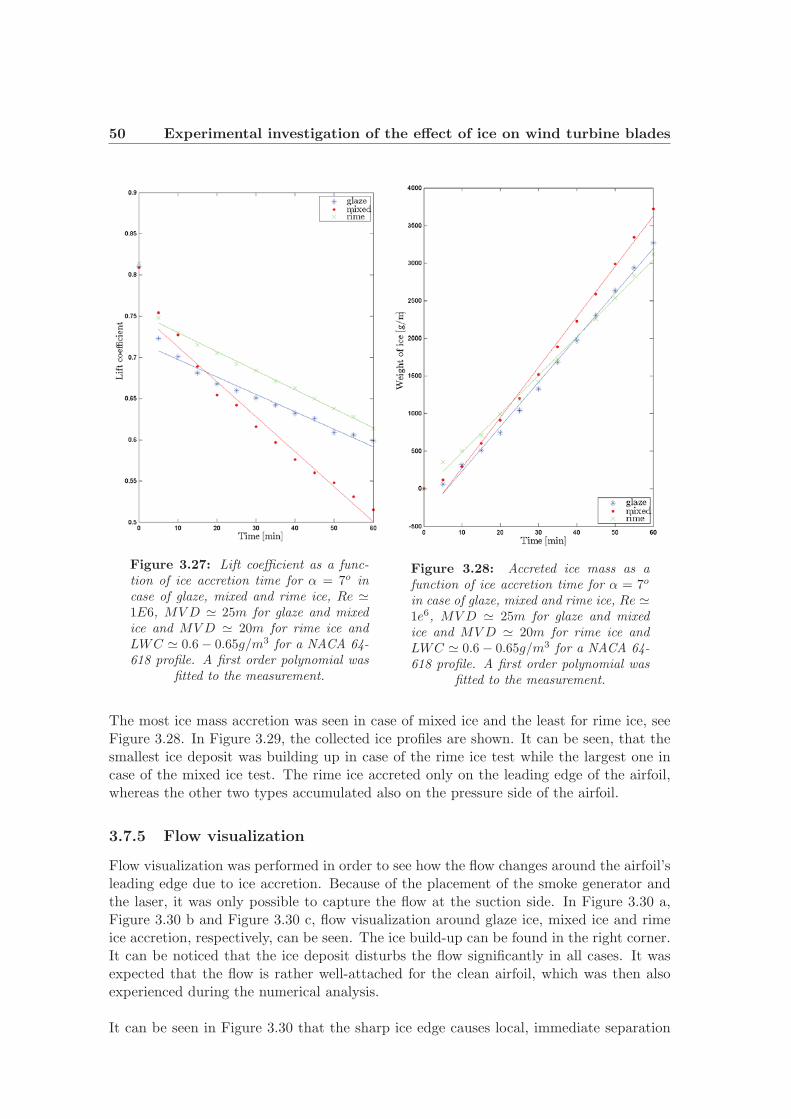
50 Experimental investigation of the effect of ice on wind turbine blades
Figure 3.27: Lift coefficient as a func-tion of ice accretion time for α = 7o incase of glaze, mixed and rime ice, Re �1E6, MVD � 25m for glaze and mixedice and MVD � 20m for rime ice andLWC � 0.6− 0.65g/m3 for a NACA 64-618 profile. A first order polynomial was
fitted to the measurement.
Figure 3.28: Accreted ice mass as afunction of ice accretion time for α = 7o
in case of glaze, mixed and rime ice, Re �1e6, MVD � 25m for glaze and mixedice and MVD � 20m for rime ice andLWC � 0.6− 0.65g/m3 for a NACA 64-618 profile. A first order polynomial was
fitted to the measurement.
The most ice mass accretion was seen in case of mixed ice and the least for rime ice, seeFigure 3.28. In Figure 3.29, the collected ice profiles are shown. It can be seen, that thesmallest ice deposit was building up in case of the rime ice test while the largest one incase of the mixed ice test. The rime ice accreted only on the leading edge of the airfoil,whereas the other two types accumulated also on the pressure side of the airfoil.
3.7.5 Flow visualization
Flow visualization was performed in order to see how the flow changes around the airfoil’sleading edge due to ice accretion. Because of the placement of the smoke generator andthe laser, it was only possible to capture the flow at the suction side. In Figure 3.30 a,Figure 3.30 b and Figure 3.30 c, flow visualization around glaze ice, mixed ice and rimeice accretion, respectively, can be seen. The ice build-up can be found in the right corner.It can be noticed that the ice deposit disturbs the flow significantly in all cases. It wasexpected that the flow is rather well-attached for the clean airfoil, which was then alsoexperienced during the numerical analysis.
It can be seen in Figure 3.30 that the sharp ice edge causes local, immediate separation
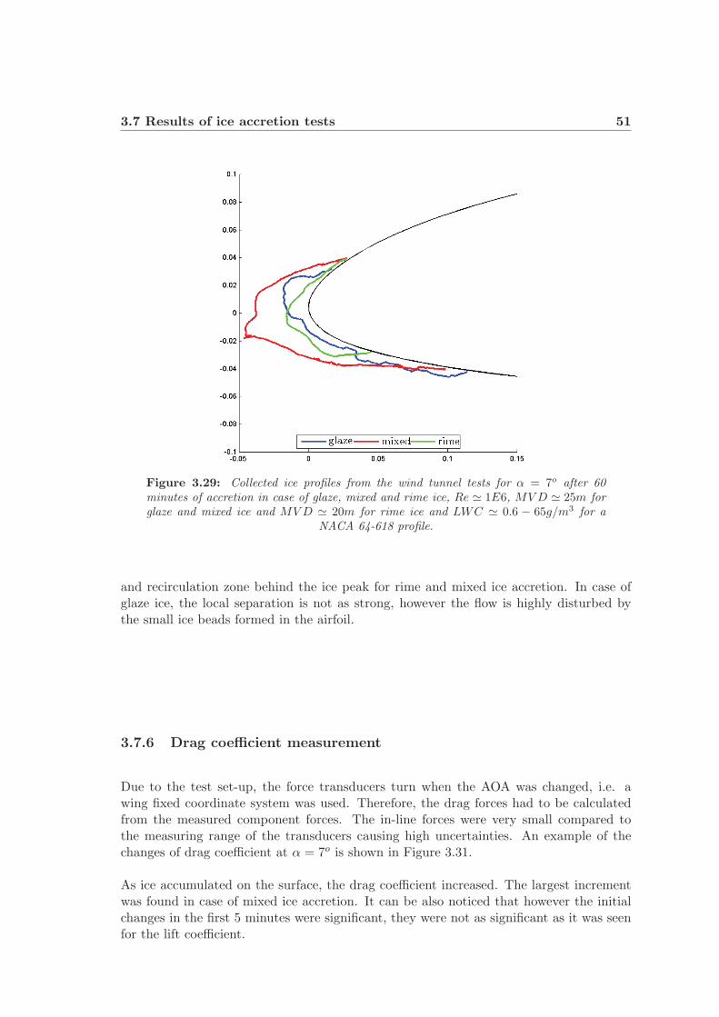
3.7 Results of ice accretion tests 51
Figure 3.29: Collected ice profiles from the wind tunnel tests for α = 7o after 60minutes of accretion in case of glaze, mixed and rime ice, Re � 1E6, MVD � 25m forglaze and mixed ice and MVD � 20m for rime ice and LWC � 0.6 − 65g/m3 for a
NACA 64-618 profile.
and recirculation zone behind the ice peak for rime and mixed ice accretion. In case ofglaze ice, the local separation is not as strong, however the flow is highly disturbed bythe small ice beads formed in the airfoil.
3.7.6 Drag coefficient measurement
Due to the test set-up, the force transducers turn when the AOA was changed, i.e. awing fixed coordinate system was used. Therefore, the drag forces had to be calculatedfrom the measured component forces. The in-line forces were very small compared tothe measuring range of the transducers causing high uncertainties. An example of thechanges of drag coefficient at α = 7o is shown in Figure 3.31.
As ice accumulated on the surface, the drag coefficient increased. The largest incrementwas found in case of mixed ice accretion. It can be also noticed that however the initialchanges in the first 5 minutes were significant, they were not as significant as it was seenfor the lift coefficient.
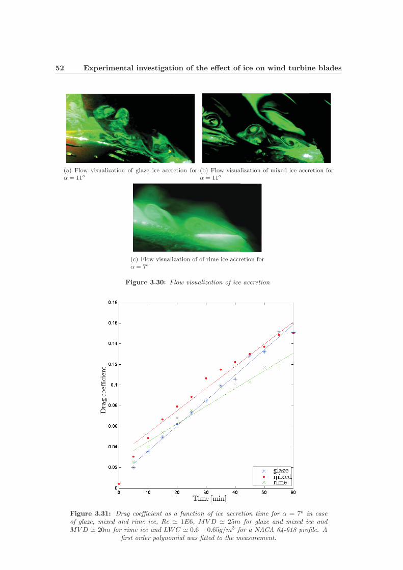
52 Experimental investigation of the effect of ice on wind turbine blades
(a) Flow visualization of glaze ice accretion forα = 11o
(b) Flow visualization of mixed ice accretion forα = 11o
(c) Flow visualization of of rime ice accretion forα = 7o
Figure 3.30: Flow visualization of ice accretion.
Figure 3.31: Drag coefficient as a function of ice accretion time for α = 7o in caseof glaze, mixed and rime ice, Re � 1E6, MVD � 25m for glaze and mixed ice andMVD � 20m for rime ice and LWC � 0.6 − 0.65g/m3 for a NACA 64-618 profile. A
first order polynomial was fitted to the measurement.
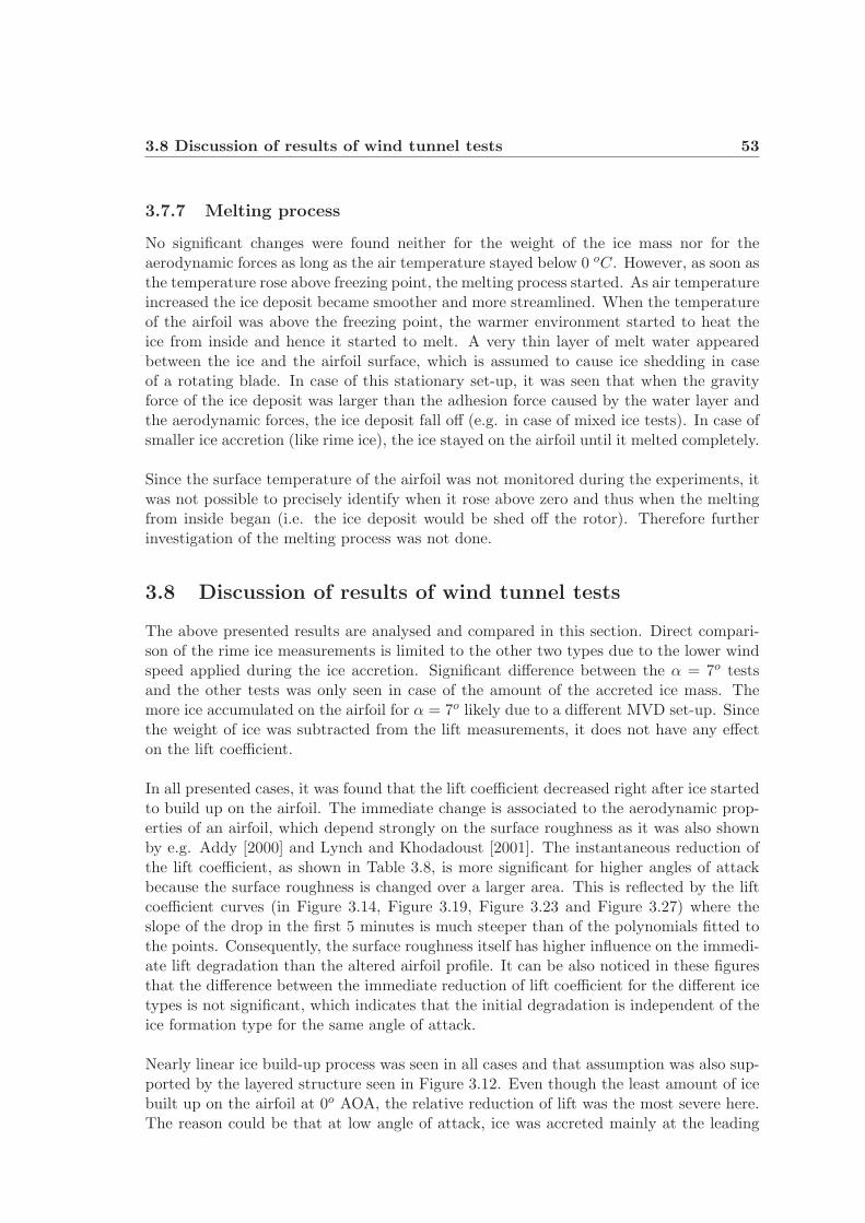
3.8 Discussion of results of wind tunnel tests 53
3.7.7 Melting process
No significant changes were found neither for the weight of the ice mass nor for theaerodynamic forces as long as the air temperature stayed below 0 oC. However, as soon asthe temperature rose above freezing point, the melting process started. As air temperatureincreased the ice deposit became smoother and more streamlined. When the temperatureof the airfoil was above the freezing point, the warmer environment started to heat theice from inside and hence it started to melt. A very thin layer of melt water appearedbetween the ice and the airfoil surface, which is assumed to cause ice shedding in caseof a rotating blade. In case of this stationary set-up, it was seen that when the gravityforce of the ice deposit was larger than the adhesion force caused by the water layer andthe aerodynamic forces, the ice deposit fall off (e.g. in case of mixed ice tests). In case ofsmaller ice accretion (like rime ice), the ice stayed on the airfoil until it melted completely.
Since the surface temperature of the airfoil was not monitored during the experiments, itwas not possible to precisely identify when it rose above zero and thus when the meltingfrom inside began (i.e. the ice deposit would be shed off the rotor). Therefore furtherinvestigation of the melting process was not done.
3.8 Discussion of results of wind tunnel tests
The above presented results are analysed and compared in this section. Direct compari-son of the rime ice measurements is limited to the other two types due to the lower windspeed applied during the ice accretion. Significant difference between the α = 7o testsand the other tests was only seen in case of the amount of the accreted ice mass. Themore ice accumulated on the airfoil for α = 7o likely due to a different MVD set-up. Sincethe weight of ice was subtracted from the lift measurements, it does not have any effecton the lift coefficient.
In all presented cases, it was found that the lift coefficient decreased right after ice startedto build up on the airfoil. The immediate change is associated to the aerodynamic prop-erties of an airfoil, which depend strongly on the surface roughness as it was also shownby e.g. Addy [2000] and Lynch and Khodadoust [2001]. The instantaneous reduction ofthe lift coefficient, as shown in Table 3.8, is more significant for higher angles of attackbecause the surface roughness is changed over a larger area. This is reflected by the liftcoefficient curves (in Figure 3.14, Figure 3.19, Figure 3.23 and Figure 3.27) where theslope of the drop in the first 5 minutes is much steeper than of the polynomials fitted tothe points. Consequently, the surface roughness itself has higher influence on the immedi-ate lift degradation than the altered airfoil profile. It can be also noticed in these figuresthat the difference between the immediate reduction of lift coefficient for the different icetypes is not significant, which indicates that the initial degradation is independent of theice formation type for the same angle of attack.
Nearly linear ice build-up process was seen in all cases and that assumption was also sup-ported by the layered structure seen in Figure 3.12. Even though the least amount of icebuilt up on the airfoil at 0o AOA, the relative reduction of lift was the most severe here.The reason could be that at low angle of attack, ice was accreted mainly at the leading
54 Experimental investigation of the effect of ice on wind turbine blades
edge, changing the geometry of the profile and thus causing higher disturbance in the flowat the suction side than at higher angles. In case of larger incident angles, the ice shapeis flatter and follows the streamlines on the pressure side, as shown in Figure 3.16, Figure3.21 and Figure 3.25, and thus induces less flow disturbance on the important suctionside. It appears that the angle of attack has an influence on the mass and also on theshape of the ice deposit. The same conclusion was drawn from the numerical simulationsby Homola et al. [2009] and Virk et al. [2010a].
Larger amount of ice built up in case of mixed ice tests compared to glaze ice tests for thesame angle of attack (except in case of 9 o, probably due to a slightly different dropletsize). It is due to the nature of the mixed ice, when the temperature reaches lower lev-els and becomes sufficiently cold for rime ice formation, all the water particles freeze onimpact, causing larger ice deposit on the already altered airfoil profile. Since the local col-lection efficiency of the airfoil’s surface is increased in the areas where ice already formed,the ice accretion process speeds up and also increases in complicity (Battisti [2009]). Thereduction of lift coefficient was more significant in case of mixed ice deposit than for glazeice. The reason could be the very irregular mixed ice shapes, which highly disturbed theflow around the airfoil.
Both Jasinski et al. [1997] and Bragg et al. [2005] pointed out that the lift coefficientbased on the original chord was sometimes higher in case of rime ice tests compared tothe clean airfoil. This behaviour was not seen during the experiments presented in thispaper probably because of different icing conditions and accretion time and thus differentice shape and size.
The mass of accreted ice highly depends on the wind speed, the temperature and liquidwater content and the droplet size [Makkonen, 1984]. The latter three parameters wereset to ensure the environmental conditions necessary for the chosen ice formation type.It was experienced that even a very small change in the droplet size led to significantlydifferent ice mass. Due to the limitations of the wind tunnel’s cooling capacity, consid-erably lower wind speed was applied than what it is acting on the tip region of a windturbine. Therefore the accumulated ice mass is less than it would have been in case ofthe outer part of a wind blade.
Although the physical characteristics of the ice deposits were similar to the one publishedin other studies e.g. Bose [1992] and ISO 12494 [2001] standard, some differences wereobserved. In case of glaze ice deposits, as it can be seen in Figure 3.18, the ice deposit isthe consists of small beads. It was seen during the experiments that the water droplets,which did not freeze on impact, formed small beads before they eventually ran off. Every5 minutes, the tunnel and the spray system was set to idle for approximately one and ahalf minutes in order to measure the weight of the accreted ice mass. Even though thisperiod is short, it could provide just enough time to get these large water droplets tofreeze. At low air speeds such as 5-10 m/s, the gravity has significant influence on thevertical deflection of the droplet trajectories, causing gravitational sedimentation (Kollaret al. [2005]), which could be the reason for the dry ice sedimentation seen on the suctionside in case of rime ice accretion during the experiment (see Figure B.3 c in Appendix B).
3.9 Conclusion drawn from the experimental study 55
In case of the mixed ice tests, the observed peak at the stagnation point in Figure 3.21and Figure 3.29 could probably be formed also due to the static feature of the tests. Thesepeaks are not experienced or have been reported yet in case of an actual rotating windturbine blade. It also has to be kept in mind that due to atmospheric turbulence, windshear, and tower passage, the angle of attack is varying in time around a mean value on awind turbine blade, which will give a broader ice accretion at the leading edge since thestagnation point is not constant.
In case of the drag coefficients, it has to be noted, that the values are very likely incorrectdue to the high uncertainties of the measurement of small forces. However, the trendof the changes of drag coefficient is as it was expected, i.e. as AOA increased, the iceaccretion caused increase in the drag because the area exposed to the wind got larger(ISO 12494 [2001]). Although there are other methods of drag force measurements, butdue to the nature of the experiments, none of them were suitable. E.g. in case of using awake rack with pressure devices would have failed because the small pressure tubes wouldvery likely have frozen immediately, making the measurements impossible.
Melting was observed during the test campaign as well. It was noticed that there wasalmost no mass changes until the air temperature was subzero. When the surface tem-perature of the airfoil rose above the freezing point, ice started to melt from ”inside”producing a thin water layer between the ice and the airfoil. At that point, the ice wouldhave shed off the blade if it was rotating, but due to the static nature of the test it wasnot.
The flow visualization confirmed that the flow was highly disturbed by the ice accretion.In Figure 3.30 b and Figure 3.30 c, the mixed and rime ice accretion can be seen, respec-tively. As a typical feature of these types of ice, ice feathers with sharp edges formed.These edges caused immediate flow separation and thus vortices and small recirculationzones at the suction side. In case of the glaze ice formation, smooth surface and thereforeless disturbance was expected, but due to small ice beads the flow pattern was disturbedquite significantly, as seen in Figure 3.30 b.
3.9 Conclusion drawn from the experimental study
In this chapter, the results of a series of experiments on a NACA 64-618 profile in aclimatic wind tunnel were presented. There were a number of tests performed at differentangles of attack and temperatures to monitor the alteration of aerodynamic forces alongwith the weight of accumulated ice throughout the first 60 minutes of ice accretion undercontrolled conditions. It was seen that all types of ice had significant negative influenceon the flow field around the airfoil. The flow visualization confirmed that the flow washighly disturbed by the ice accretion. Both the ice accretion and the lift coefficientdegradation showed a nearly linear trend. The alteration of the surface roughness has amore significant influence on the initial lift coefficient than the shape of the changed airfoilprofile. As the angle of attack increased the larger the degradation of the instantaneouslift coefficient got.
It was also found, that not only the temperature, but also the angle of attack has an

56 Experimental investigation of the effect of ice on wind turbine blades
influence on the mass and also the shape of ice deposit. Even though the least amountof ice built up on the airfoil at low angles of attack, the relative reduction was the mostsevere in these cases, i.e. the higher the angle of attack the lower the relative lift coefficientdegradation.
The importance of MVD was experienced when a small, accidental change caused out oftrend ice mass accretion on the airfoil. More ice built up on the airfoil during the mixedice tests than during the glaze ice tests and hence caused more significant lift coefficientdegradation.
Similarly to previous studies, the shape and mass of ice deposits were found to be highlydependent of LWC, MVD and temperature. Although most of the physical characteristicswere in good agreement with the expectations based on other studies and standards, therewere some differences observed. During glaze ice accretion, tiny ice beads froze to thesurface and in case of mixed ice, a sharp nose-like ice peak formed around the stagnationpoint. It is suspected that both formation occurred due to the nature of the wind tunneltests.
The changes of drag coefficient was monitored as well. The increase was found to be alsoa nearly linear process for all ice types. It is, however, suspected that the measured valuesare much higher due to the measurement range of the used transducers.
It can be concluded that even one hour of ice accretion has significant influence on theaerodynamics of the airfoil and the angle of attack at which the ice builds up on thesurface is highly important.
In order to be able to properly study the impact of ice on drag force, a more suitablemeasuring system is needed, which is either heated so it could handle the impacts of iceor is a different force transducer, which has a better response to low forces. An infra-redcamera would be very useful to study the mechanism of melting. In that way the surfacetemperature of the ice and the airfoil would be followed.

Chapter 4
Numerical investigation of icing ofwind turbine blades
In this chapter a numerical investigation of the impact from ice accumulation on windturbine blades is presented. As it was mentioned in the previous chapter, ice profiles werecollected for further numerical analysis during the wind tunnel tests. They were directlycompared to results of the dedicated ice simulation model, TURBICE from VTT, Tech-nical Research Centre of Finland in order to validate the ice shapes and to calibrate thewind tunnel parameters for LWC and MVD. The collected profiles were also used to nu-merically analyse the impacts of ice accretion on the flow behaviour and the aerodynamiccharacteristics of the airfoil using Ansys Fluent. This chapter gives a short summary ofthe most relevant publications in the field and details the set-up and results of the presentnumerical study.
4.1 Introduction to numerical investigation
In the recent years, especially due to the tremendous increase in computing power, CFDsimulations, even in 3D, has become much faster. It is now also possible to some degreeestimate the shape and mass of ice deposit on airfoils and thus determine the performanceof an iced wind turbine more punctual than earlier. The ice accretion models have beenimproved and the impacts of ice on wind turbine behaviour are also known better by now(Makkonen et al. [2001]), but there are still several issues and unsolved problems when itcomes to the prediction of ice risk and production loss.
There are presently dedicated ice accretion models available on the field. One of the mostwell-known model is Nasa’s LEWICE, which is built up of four modules; potential flowfield calculation, particle trajectory and impingement calculation, thermodynamic andice growth calculation, and finally the geometry modification due to ice growth. The iceaccretion itself is a time-stepping procedure (Wright et al. [2008]). Another, comprehen-sive numerical ice accretion software is TURBICE from VTT Technical Research Centreof Finland, which also uses the panel method to calculate the potential flow (Makko-nen et al. [2001]). The results have been verified by icing wind tunnel testing of bothaircraft and wind turbine airfoils (Homola et al. [2010b]). Fensap-ICE is an aerodynam-ics and icing simulation system from Newmerical Technologies International (NTI). Thismodel was developed for solving aeronautic issues, however it has been recently used inwind energy applications (Virk et al. [2010b], Virk et al. [2012] and Reid et al. [2013]).
58 Numerical investigation of icing of wind turbine blades
There are three modules set in a loop; the flow field calculation using the compressibleNavier-Stokes equations with FENSAP (or other solvers), the computation of the collec-tion efficiency distribution with DROP3D, and then the prediction of the ice accretionshape by a shallow-water icing model with ICE3D (Habashi et al. [2001]).
Simulations with computational fluid dynamics (CFD) based techniques are used to nu-merically analyze the impacts of ice accretion on the flow behavior and the aerodynamiccharacteristics of the airfoil. The analysis can be done using either an individual CFDprogram, e.g. Ansys Fluent, or aerodynamics and icing simulation program with built-inCFD module such as Fensap-ICE.
In some recent studies, the numerical simulations were carried out in two steps (e.g. Virket al. [2010a], Etemaddar et al. [2012]). In the first step, the physical characteristics ofthe accreted ice (e.g. shape and size) were predicted with one of the above described iceaccretion models. In the second step, CFD analyses were performed on the iced airfoilto estimate the effect on drag and lift forces. Homola et al. [2010a] combined TURBICEand Ansys Fluent to investigate the effect of ice on a NACA 64-618 profile. The ice pro-files were the results of three different droplet sizes and air temperatures and they wereanalysed at different angles of attack ranging from −10o to +20o. The lift coefficient wasfound to be reduced in all cases and the smallest change was observed in case of stream-lined rime ice, while there was larger reduction experienced with horn shaped glaze ice.During the CFD simulations, it was found that the horn type glaze ice caused the largestseparation, and thus significant lift reduction and higher drag coefficient.
Etemaddar et al. [2012] was also using a NACA 64-618 in their numerical analysis, how-ever instead of TURBICE, they used LEWICE. It was found that the ice load increaseswith liquid water content (LWC), median volume diameter (MVD) and relative windspeed.
Two 2-D studies (Virk et al. [2010b] and Virk et al. [2012]) have been carried out usingFensap-ICE. Virk et al. [2010b] studied only one section with different angles of attackand atmospheric temperatures, whereas Virk et al. [2012] selected five sections along theblade radius, thereby each tests were performed with different angle of attacks and rela-tive wind speeds. The results showed that the angle of attack has influence on the rateand shape of ice growth and for lower angle of attacks the icing is less severe near to thetip (Virk et al. [2010b]).
Recently, a 3D study was done with Fensap-ICE by Reid et al. [2013]. They pointed outthat the largest performance degradations were seen at lower wind speed, where the icedeposit caused small separations in places where it was not experienced with the cleanprofile.
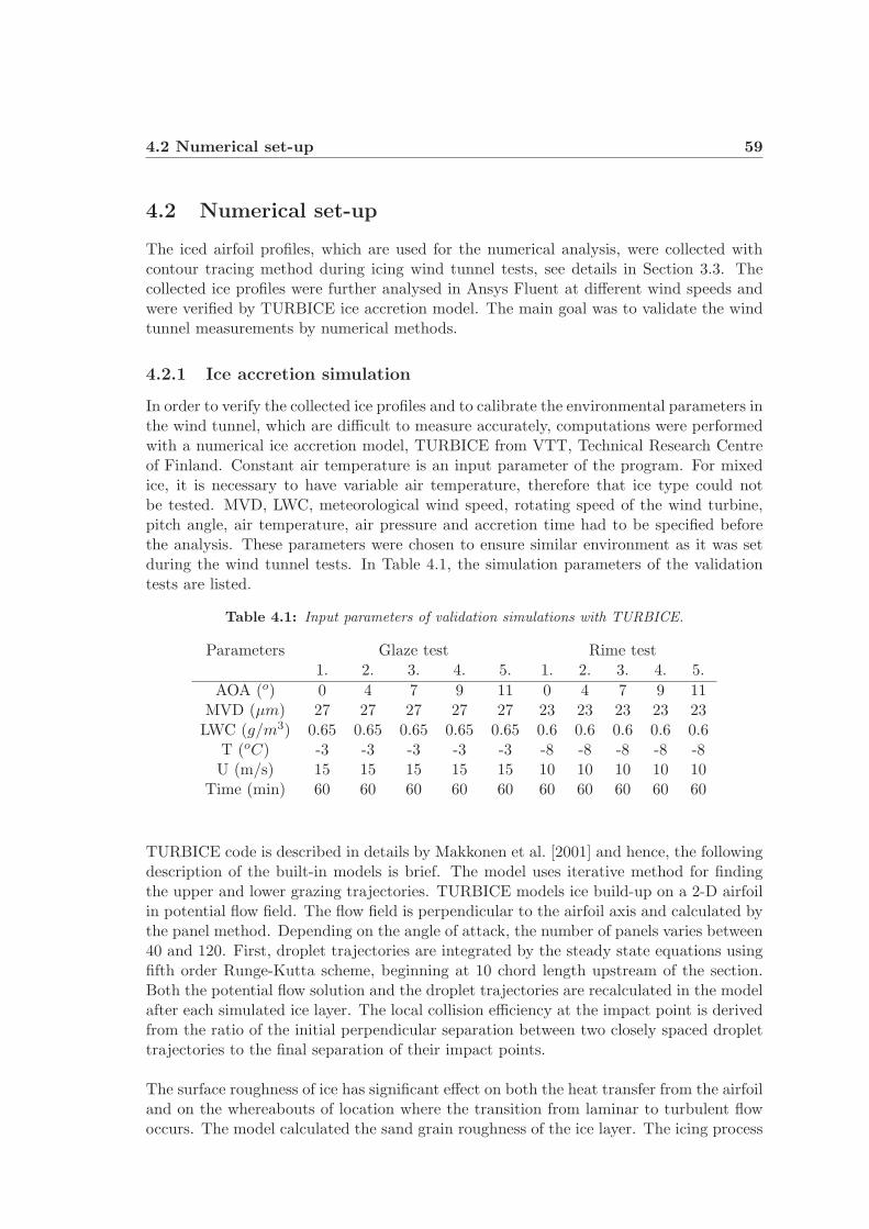
4.2 Numerical set-up 59
4.2 Numerical set-up
The iced airfoil profiles, which are used for the numerical analysis, were collected withcontour tracing method during icing wind tunnel tests, see details in Section 3.3. Thecollected ice profiles were further analysed in Ansys Fluent at different wind speeds andwere verified by TURBICE ice accretion model. The main goal was to validate the windtunnel measurements by numerical methods.
4.2.1 Ice accretion simulation
In order to verify the collected ice profiles and to calibrate the environmental parameters inthe wind tunnel, which are difficult to measure accurately, computations were performedwith a numerical ice accretion model, TURBICE from VTT, Technical Research Centreof Finland. Constant air temperature is an input parameter of the program. For mixedice, it is necessary to have variable air temperature, therefore that ice type could notbe tested. MVD, LWC, meteorological wind speed, rotating speed of the wind turbine,pitch angle, air temperature, air pressure and accretion time had to be specified beforethe analysis. These parameters were chosen to ensure similar environment as it was setduring the wind tunnel tests. In Table 4.1, the simulation parameters of the validationtests are listed.
Table 4.1: Input parameters of validation simulations with TURBICE.
Parameters Glaze test Rime test1. 2. 3. 4. 5. 1. 2. 3. 4. 5.
AOA (o) 0 4 7 9 11 0 4 7 9 11MVD (μm) 27 27 27 27 27 23 23 23 23 23LWC (g/m3) 0.65 0.65 0.65 0.65 0.65 0.6 0.6 0.6 0.6 0.6
T (oC) -3 -3 -3 -3 -3 -8 -8 -8 -8 -8U (m/s) 15 15 15 15 15 10 10 10 10 10
Time (min) 60 60 60 60 60 60 60 60 60 60
TURBICE code is described in details by Makkonen et al. [2001] and hence, the followingdescription of the built-in models is brief. The model uses iterative method for findingthe upper and lower grazing trajectories. TURBICE models ice build-up on a 2-D airfoilin potential flow field. The flow field is perpendicular to the airfoil axis and calculated bythe panel method. Depending on the angle of attack, the number of panels varies between40 and 120. First, droplet trajectories are integrated by the steady state equations usingfifth order Runge-Kutta scheme, beginning at 10 chord length upstream of the section.Both the potential flow solution and the droplet trajectories are recalculated in the modelafter each simulated ice layer. The local collision efficiency at the impact point is derivedfrom the ratio of the initial perpendicular separation between two closely spaced droplettrajectories to the final separation of their impact points.
The surface roughness of ice has significant effect on both the heat transfer from the airfoiland on the whereabouts of location where the transition from laminar to turbulent flowoccurs. The model calculated the sand grain roughness of the ice layer. The icing process
60 Numerical investigation of icing of wind turbine blades
itself is time-dependent. The time dependency in the roughness model is accounted for themultiplication factor, which depends on the freezing point, and the number of simulatedice layers.
In order to calculate the heat and mass transfer, the surface of the airfoil section is dividedinto finite areas. The mass and energy balance of these areas are used to determinethe freezing fraction and the surface temperature. When the freezing fraction is zero,ice does not form, whereas when it is unity, rime ice accretes on the surface. In theenergy balance, TURBICE takes into account convection, evaporation, droplet heating,IR radiation, friction and heat contained in the runback water. Based on the local valuesof ice mass flux and density, the local ice thickness and thus ice layers can be calculatedin a small time step.
The growth direction of rime ice is the mean direction of arrival of the droplet trajectories.In case of glaze ice the growth direction depends on the freezing factor, e.g. when it tendsto unity the growth direction is the same as in rime icing. In the runback area, the icegrows perpendicular to the local area.
4.2.2 Computational fluid dynamics
Simulations with Ansys Fluent were conducted to quantify the impacts of ice accretionon the flow behavior and the aerodynamic characteristics of the iced airfoil from the windtunnel tests. First, the aerodynamic forces measured during the experiments were veri-fied. Due to the limitation of the CWT’s cooling unit, it was necessary to set relativelylow target wind speed (15 m/s which corresponds to approximately Re � 1E6) to ensurestable and low enough air temperature. A number of numerical tests were performed withhigher wind speeds, i.e. 25 m/s (Re � 1.5E6) and 40 m/s (Re � 2.5E6) as well. Foreach simulation, profiles with ice deposit accreted at the same AOA as the investigationof the flow behaviour and the aerodynamic characteristics were done, were used. Thesetests are referred as ”dedicated profile” tests or simulations.
The impact of angle of attack was investigated with one single ice profile. For this inves-tigation, the glaze and rime iced airfoils collected at α = 0o and 11o were chosen and theywere tested in flows with 0o, 4o, 7o, 9o and 11o incident angles and 25 m/s wind speed.These tests are referred as ”single profile” tests or simulations.
The ice profiles were collected from specific spanwise locations, and therefore 2-D modelswere constructed in Ansys Workbench. The control volume around the airfoil was rectan-gular with edges positioned at 50 chords length away in vertical direction and 20 chordslength from the horizontal direction.
An inflation layer was added to the mesh to produce a structured, fine mesh in the vicinityof the airfoil (see Figure 4.1) to achieve the desired wall Y + distribution and thus to givea better representation of the flow near the airfoil surface. The first layer height is depen-dent on the surface roughness, since the roughness height may not exceed it. However,it was experienced that Ansys Fluent cannot properly handle micro surface roughness,therefore it was not included in the analysis, see detailed explanation in the next section.
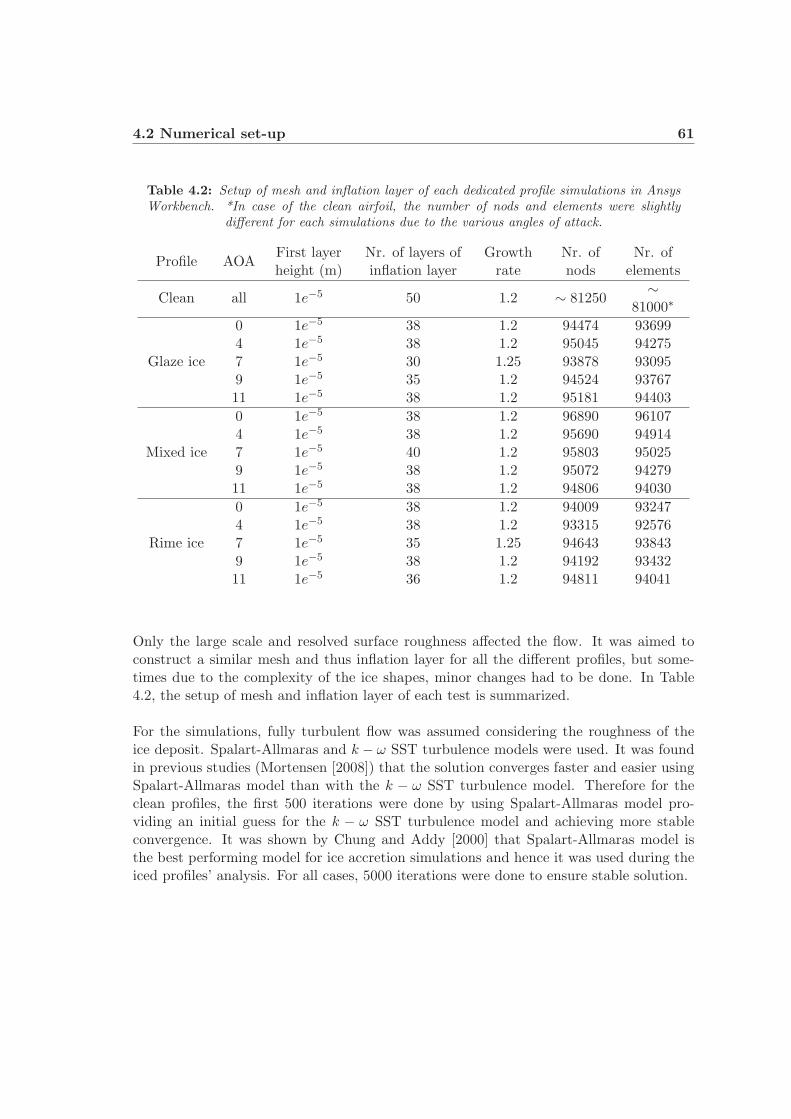
4.2 Numerical set-up 61
Table 4.2: Setup of mesh and inflation layer of each dedicated profile simulations in AnsysWorkbench. *In case of the clean airfoil, the number of nods and elements were slightly
different for each simulations due to the various angles of attack.
Profile AOAFirst layerheight (m)
Nr. of layers ofinflation layer
Growthrate
Nr. ofnods
Nr. ofelements
Clean all 1e−5 50 1.2 ∼ 81250∼
81000∗
Glaze ice
0 1e−5 38 1.2 94474 936994 1e−5 38 1.2 95045 942757 1e−5 30 1.25 93878 930959 1e−5 35 1.2 94524 9376711 1e−5 38 1.2 95181 94403
Mixed ice
0 1e−5 38 1.2 96890 961074 1e−5 38 1.2 95690 949147 1e−5 40 1.2 95803 950259 1e−5 38 1.2 95072 9427911 1e−5 38 1.2 94806 94030
Rime ice
0 1e−5 38 1.2 94009 932474 1e−5 38 1.2 93315 925767 1e−5 35 1.25 94643 938439 1e−5 38 1.2 94192 9343211 1e−5 36 1.2 94811 94041
Only the large scale and resolved surface roughness affected the flow. It was aimed toconstruct a similar mesh and thus inflation layer for all the different profiles, but some-times due to the complexity of the ice shapes, minor changes had to be done. In Table4.2, the setup of mesh and inflation layer of each test is summarized.
For the simulations, fully turbulent flow was assumed considering the roughness of theice deposit. Spalart-Allmaras and k − ω SST turbulence models were used. It was foundin previous studies (Mortensen [2008]) that the solution converges faster and easier usingSpalart-Allmaras model than with the k − ω SST turbulence model. Therefore for theclean profiles, the first 500 iterations were done by using Spalart-Allmaras model pro-viding an initial guess for the k − ω SST turbulence model and achieving more stableconvergence. It was shown by Chung and Addy [2000] that Spalart-Allmaras model isthe best performing model for ice accretion simulations and hence it was used during theiced profiles’ analysis. For all cases, 5000 iterations were done to ensure stable solution.
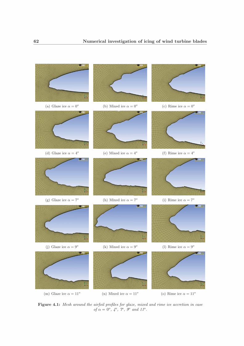
62 Numerical investigation of icing of wind turbine blades
(a) Glaze ice α = 0o (b) Mixed ice α = 0o (c) Rime ice α = 0o
(d) Glaze ice α = 4o (e) Mixed ice α = 4o (f) Rime ice α = 4o
(g) Glaze ice α = 7o (h) Mixed ice α = 7o (i) Rime ice α = 7o
(j) Glaze ice α = 9o (k) Mixed ice α = 9o (l) Rime ice α = 9o
(m) Glaze ice α = 11o (n) Mixed ice α = 11o (o) Rime ice α = 11o
Figure 4.1: Mesh around the airfoil profiles for glaze, mixed and rime ice accretion in caseof α = 0o, 4o, 7o, 9o and 11o.
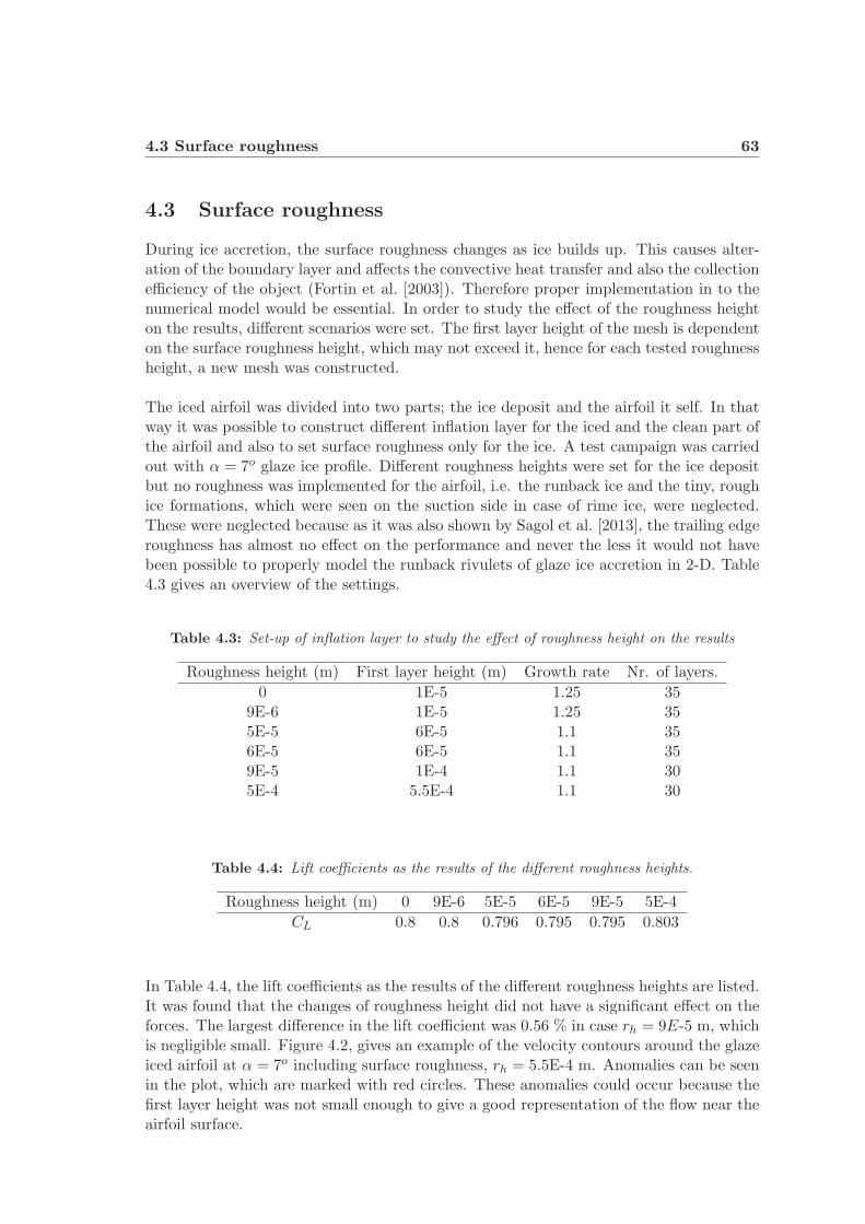
4.3 Surface roughness 63
4.3 Surface roughness
During ice accretion, the surface roughness changes as ice builds up. This causes alter-ation of the boundary layer and affects the convective heat transfer and also the collectionefficiency of the object (Fortin et al. [2003]). Therefore proper implementation in to thenumerical model would be essential. In order to study the effect of the roughness heighton the results, different scenarios were set. The first layer height of the mesh is dependenton the surface roughness height, which may not exceed it, hence for each tested roughnessheight, a new mesh was constructed.
The iced airfoil was divided into two parts; the ice deposit and the airfoil it self. In thatway it was possible to construct different inflation layer for the iced and the clean part ofthe airfoil and also to set surface roughness only for the ice. A test campaign was carriedout with α = 7o glaze ice profile. Different roughness heights were set for the ice depositbut no roughness was implemented for the airfoil, i.e. the runback ice and the tiny, roughice formations, which were seen on the suction side in case of rime ice, were neglected.These were neglected because as it was also shown by Sagol et al. [2013], the trailing edgeroughness has almost no effect on the performance and never the less it would not havebeen possible to properly model the runback rivulets of glaze ice accretion in 2-D. Table4.3 gives an overview of the settings.
Table 4.3: Set-up of inflation layer to study the effect of roughness height on the results
Roughness height (m) First layer height (m) Growth rate Nr. of layers.
0 1E-5 1.25 359E-6 1E-5 1.25 355E-5 6E-5 1.1 356E-5 6E-5 1.1 359E-5 1E-4 1.1 305E-4 5.5E-4 1.1 30
Table 4.4: Lift coefficients as the results of the different roughness heights.
Roughness height (m) 0 9E-6 5E-5 6E-5 9E-5 5E-4
CL 0.8 0.8 0.796 0.795 0.795 0.803
In Table 4.4, the lift coefficients as the results of the different roughness heights are listed.It was found that the changes of roughness height did not have a significant effect on theforces. The largest difference in the lift coefficient was 0.56 % in case rh = 9E-5 m, whichis negligible small. Figure 4.2, gives an example of the velocity contours around the glazeiced airfoil at α = 7o including surface roughness, rh = 5.5E-4 m. Anomalies can be seenin the plot, which are marked with red circles. These anomalies could occur because thefirst layer height was not small enough to give a good representation of the flow near theairfoil surface.
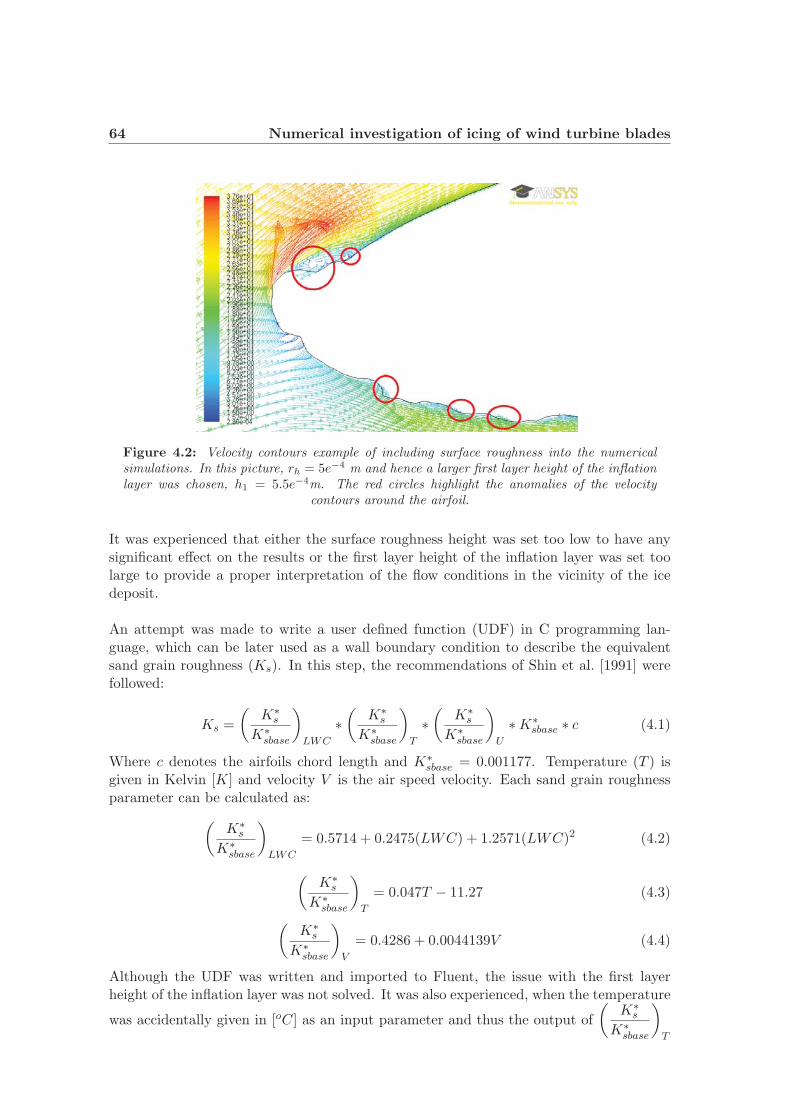
64 Numerical investigation of icing of wind turbine blades
Figure 4.2: Velocity contours example of including surface roughness into the numericalsimulations. In this picture, rh = 5e−4 m and hence a larger first layer height of the inflationlayer was chosen, h1 = 5.5e−4m. The red circles highlight the anomalies of the velocity
contours around the airfoil.
It was experienced that either the surface roughness height was set too low to have anysignificant effect on the results or the first layer height of the inflation layer was set toolarge to provide a proper interpretation of the flow conditions in the vicinity of the icedeposit.
An attempt was made to write a user defined function (UDF) in C programming lan-guage, which can be later used as a wall boundary condition to describe the equivalentsand grain roughness (Ks). In this step, the recommendations of Shin et al. [1991] werefollowed:
Ks =
(K∗
s
K∗sbase
)LWC
∗(
K∗s
K∗sbase
)T
∗(
K∗s
K∗sbase
)U
∗K∗sbase ∗ c (4.1)
Where c denotes the airfoils chord length and K∗sbase = 0.001177. Temperature (T ) is
given in Kelvin [K] and velocity V is the air speed velocity. Each sand grain roughnessparameter can be calculated as:(
K∗s
K∗sbase
)LWC
= 0.5714 + 0.2475(LWC) + 1.2571(LWC)2 (4.2)
(K∗
s
K∗sbase
)T
= 0.047T − 11.27 (4.3)
(K∗
s
K∗sbase
)V
= 0.4286 + 0.0044139V (4.4)
Although the UDF was written and imported to Fluent, the issue with the first layerheight of the inflation layer was not solved. It was also experienced, when the temperature
was accidentally given in [oC] as an input parameter and thus the output of
(K∗
s
K∗sbase
)T

4.4 Results of numerical investigation 65
became negative and so did Ks. However, there was not any error messages given byFluent and the simulation could run without any problem, which clearly indicates theissues with the roughness handling of Fluent.
Based on these results and experiences, it was decided not to implement the micro surfaceroughness in order to be able to properly simulate the flow conditions close to the airfoiland ice surface and to ensure the validity of the log law.
4.4 Results of numerical investigation
4.4.1 Ice accretion simulation
The aim of the TURBICE tests was to validate the collected ice profiles and the settingof the meteorological variables, especially MVD and LWC. Therefore a set of simulationswere performed using the same input parameters as the target values of the wind tunneltests. In Figure 4.3, the TURBICE profiles are plotted against the experimental ones forglaze and rime ice for α = 0o (the profiles of the other four angles of attack can be foundin Appendix D).
(a) Glaze ice accretion α = 0o (b) Rime ice accretion α = 0o
Figure 4.3: Results of TURBICE simulation plotted against the profiles from the wind tunneltests for both glaze and rime ice accretion at α = 0o.
As it can be seen in these plots, the numerical profiles are significantly smaller than theones from the wind tunnel, which indicates underestimation of the input parameters,especially the MVD.
Therefore additional simulations were performed in order to find the valid combinationof LWC and MVD. The first TURBICE tests run with 90 minutes accretion time, butafter the first wind tunnel experiment, it was obvious that 60 minutes accretion time islong enough to produce significant amount of ice on the airfoil and considerably reducethe lift coefficient. Therefore the accretion time in TURBICE had to be also reduced.However the already collected 90 minutes data could provide help in finding the valid
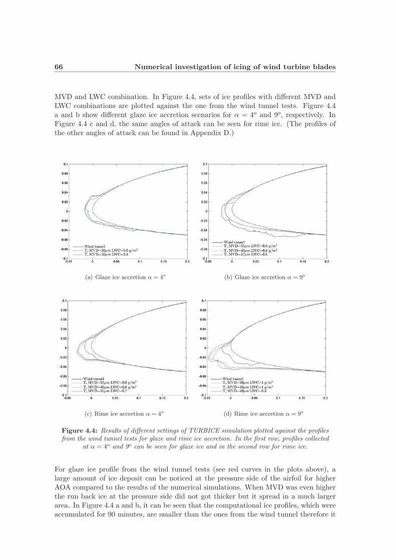
66 Numerical investigation of icing of wind turbine blades
MVD and LWC combination. In Figure 4.4, sets of ice profiles with different MVD andLWC combinations are plotted against the one from the wind tunnel tests. Figure 4.4a and b show different glaze ice accretion scenarios for α = 4o and 9o, respectively. InFigure 4.4 c and d, the same angles of attack can be seen for rime ice. (The profiles ofthe other angles of attack can be found in Appendix D.)
(a) Glaze ice accretion α = 4o (b) Glaze ice accretion α = 9o
(c) Rime ice accretion α = 4o (d) Rime ice accretion α = 9o
Figure 4.4: Results of different settings of TURBICE simulation plotted against the profilesfrom the wind tunnel tests for glaze and rime ice accretion. In the first row, profiles collected
at α = 4o and 9o can be seen for glaze ice and in the second row for rime ice.
For glaze ice profile from the wind tunnel tests (see red curves in the plots above), alarge amount of ice deposit can be noticed at the pressure side of the airfoil for higherAOA compared to the results of the numerical simulations. When MVD was even higherthe run back ice at the pressure side did not got thicker but it spread in a much largerarea. In Figure 4.4 a and b, it can be seen that the computational ice profiles, which wereaccumulated for 90 minutes, are smaller than the ones from the wind tunnel therefore it

4.4 Results of numerical investigation 67
was decided to continue the investigation only with rime ice profile.
The results gave the best fits for all angles of attack for rime ice accretion with LWC �1g/m3 and MVD � 40μm and rather than 0.6 g/m3 and 23μm, as specified by themanufacturer of the spray nozzles based on the setted water and air pressure. It isassumed that for glaze ice, MVD and LWC are higher than these values because of theslightly different settings.
4.4.2 Computational fluid dynamics
There have been in all 60 dedicated profile simulations performed with Ansys Fluent,including clean, glaze iced, mixed iced and rime iced airfoils with different wind speeds(15 m/s, 25 m/s and 40 m/s). 15 m/s wind speed was chosen to simulate similar flowconditions as in the wind tunnel to compare the results directly. Higher wind speeds wereinvestigated to see the influence of ice on the lift coefficient for more realistic situations.
Table 4.5 summarises the lift coefficients for the clean profiles for different wind speeds.Comparing these results to the wind tunnel measurements, it is indicated that the verticalwalls had significant influence on the measurement. It can be seen that the numericalanalysis gave 20 % higher lift coefficients. This suggests that the effective airfoil span is20 % shorter than the geometric span, i.e. it is approximately 1.08 m instead of 1.35 m.Based on this information, the measured lift coefficients are corrected in Table 4.6. Theuncorrected results are presented in the previous chapter, see Table 3.8.
Table 4.5: Lift coefficient of the clean airfoils for different wind speeds from Ansys Fluentsimulations.
U αm/s 0o 4o 7o 9o 11o
CL
15 0.38 0.76 1.01 1.15 1.2825 0.39 0.78 1.07 1.16 1.2740 0.39 0.79 1.1 1.18 1.29
The lift coefficients and the relative changes caused by the iced airfoil are listed in Table4.7. Comparing the different ice types, the most significant lift degradation was foundfor mixed ice tests and the smallest for rime ice for most cases. The lowest lift reductionwas found at lower angles of attack. For glaze and rime ice tests, the largest relativechange was seen at α = 9o and for mixed ice tests, at α = 7o. Comparing the relative liftcoefficient reduction to the ones in Table 4.6, it can be seen that much higher reductionwas found during the experiments.
In Figure 4.5, the results achieved at 15 m/s wind speed, are plotted against the onesfrom the wind tunnel tests for the dedicated profile tests. It can be seen, that howeverthe values collected during the wind tunnel tests are much lower than the ones fromthe numerical analysis, the trend of these curves is similar to the numerical one. Thestreamlines and the velocity distribution around the clean airfoil for different angles ofattack are plotted in Figure 4.6 and Figure 4.7, respectively. The results for ice cases

68 Numerical investigation of icing of wind turbine blades
Table 4.6: Corrected wind tunnel lift measurements. The presence of the vertical walls andend plates reduced the effective chord width with 20 %.
Glaze iceAOA 0o 4o 7o 9o 11o
CL0 (clean airfoil) 0.40 0.70 1.01 1.13 1.30CLf (final, iced airfoil) 0.20 0.46 0.64 0.80 1.01
Degradation [%] 50 35 36 29 22Mixed ice
AOA 0o 4o 7o 9o 11o
CL0 (clean airfoil) 0.40 0.72 1.01 1.14 1.30CLf (final, iced airfoil) 0.15 0.39 0.64 0.75 1.07
Degradation [%] 64 47 36 35 18Rime ice
AOA 0o 4o 7o 9o 11o
CL0 (clean airfoil) 0.40 0.71 1.02 1.20 1.33CLf (final, iced airfoil) 0.23 0.54 0.77 0.93 1.01
Degradation [%] 42 25 25 23 24
Table 4.7: Lift coefficients and relative changes for the iced airfoils for the dedicated profiletests from Ansys Fluent simulations.
U Glaze iced profile(m/s) 0o 4o 7o 9o 11o
CL
15 0.35 0.6 0.78 0.84 0.9225 0.33 0.6 0.8 0.85 0.9440 0.35 0.61 0.81 0.85 0.92
CL change (%)15 11 21 22 27 2525 11 23 25 28 2840 9 23 24 28 28U Mixed iced profile
(m/s) 0o 4o 7o 9o 11o
CL
15 0.33 0.57 0.75 0.89 1.0225 0.34 0.57 0.75 0.9 0.9940 0.34 0.58 0.76 0.9 1
CL change (%)15 12 26 26 22 2025 15 27 29 23 2240 13 27 28 24 22U Rime iced profile
(m/s) 0o 4o 7o 9o 11o
CL
15 0.35 0.62 0.83 0.93 1.0625 0.35 0.62 0.84 0.94 1.0240 0.35 0.63 0.84 0.95 1.03
CL change (%)15 8 19 18 19 1725 10 20 22 19 1940 9 21 20 19 20
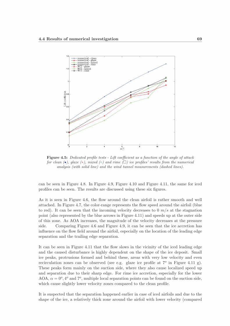
4.4 Results of numerical investigation 69
Figure 4.5: Dedicated profile tests - Lift coefficient as a function of the angle of attackfor clean (•), glaze (∗), mixed (◦) and rime (�) ice profiles’ results from the numerical
analysis (with solid line) and the wind tunnel measurements (dashed lines).
can be seen in Figure 4.8. In Figure 4.9, Figure 4.10 and Figure 4.11, the same for icedprofiles can be seen. The results are discussed using these six figures.
As it is seen in Figure 4.6, the flow around the clean airfoil is rather smooth and wellattached. In Figure 4.7, the color-range represents the flow speed around the airfoil (blueto red). It can be seen that the incoming velocity decreases to 0 m/s at the stagnationpoint (also represented by the blue arrows in Figure 4.11) and speeds up at the outer sideof this zone. As AOA increases, the magnitude of the velocity decreases at the pressureside. Comparing Figure 4.6 and Figure 4.9, it can be seen that the ice accretion hasinfluence on the flow field around the airfoil, especially on the location of the leading edgeseparation and the trailing edge separation.
It can be seen in Figure 4.11 that the flow slows in the vicinity of the iced leading edgeand the caused disturbance is highly dependent on the shape of the ice deposit. Smallice peaks, protrusions formed and behind these, areas with very low velocity and evenrecirculation zones can be observed (see e.g. glaze ice profile at 7o in Figure 4.11 g).These peaks form mainly on the suction side, where they also cause localized speed upand separation due to their sharp edge. For rime ice accretion, especially for the lowerAOA, α = 0o, 4o and 7o, multiple local separation points can be found on the suction side,which cause slightly lower velocity zones compared to the clean profile.
It is suspected that the separation happened earlier in case of iced airfoils and due to theshape of the ice, a relatively thick zone around the airfoil with lower velocity (compared
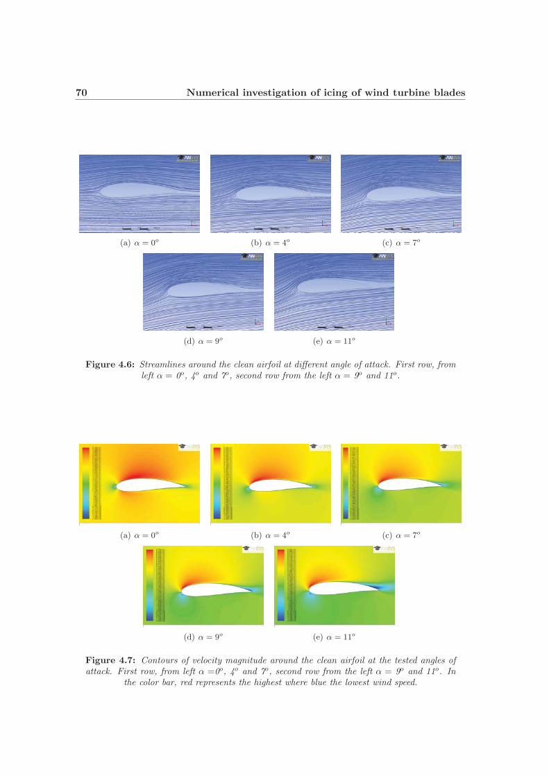
70 Numerical investigation of icing of wind turbine blades
(a) α = 0o (b) α = 4o (c) α = 7o
(d) α = 9o (e) α = 11o
Figure 4.6: Streamlines around the clean airfoil at different angle of attack. First row, fromleft α = 0o, 4o and 7o, second row from the left α = 9o and 11o.
(a) α = 0o (b) α = 4o (c) α = 7o
(d) α = 9o (e) α = 11o
Figure 4.7: Contours of velocity magnitude around the clean airfoil at the tested angles ofattack. First row, from left α =0o, 4o and 7o, second row from the left α = 9o and 11o. In
the color bar, red represents the highest where blue the lowest wind speed.
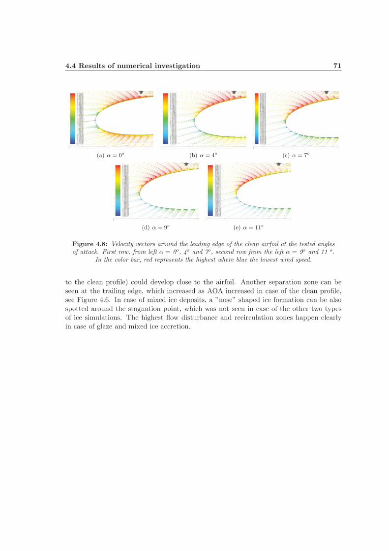
4.4 Results of numerical investigation 71
(a) α = 0o (b) α = 4o (c) α = 7o
(d) α = 9o (e) α = 11o
Figure 4.8: Velocity vectors around the leading edge of the clean airfoil at the tested anglesof attack. First row, from left α = 0o, 4o and 7o, second row from the left α = 9o and 11 o.
In the color bar, red represents the highest where blue the lowest wind speed.
to the clean profile) could develop close to the airfoil. Another separation zone can beseen at the trailing edge, which increased as AOA increased in case of the clean profile,see Figure 4.6. In case of mixed ice deposits, a ”nose” shaped ice formation can be alsospotted around the stagnation point, which was not seen in case of the other two typesof ice simulations. The highest flow disturbance and recirculation zones happen clearlyin case of glaze and mixed ice accretion.
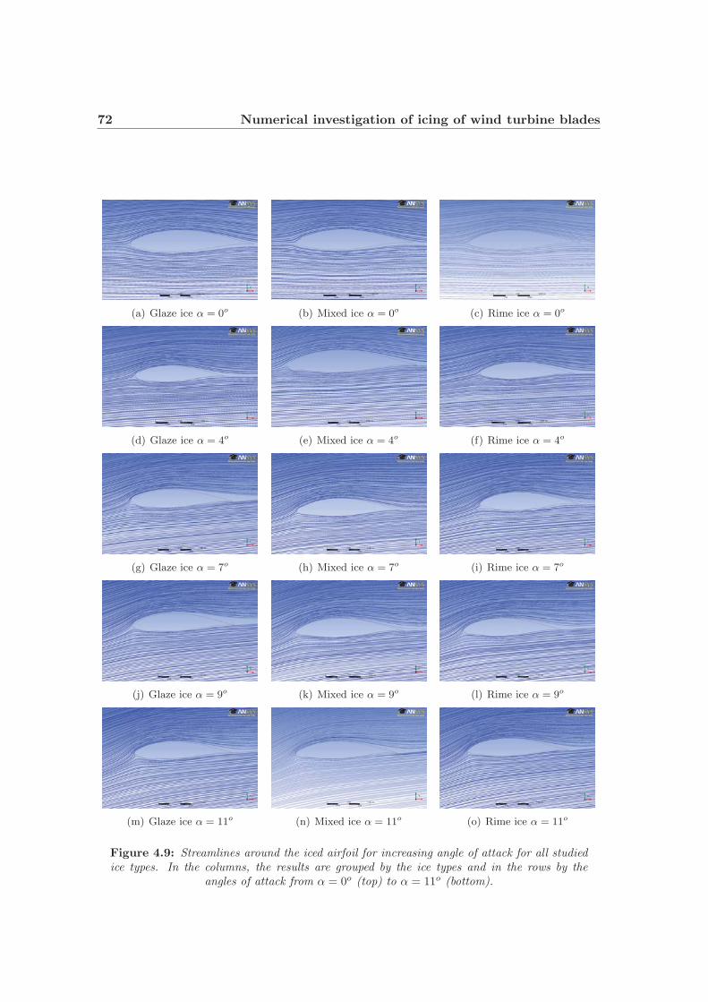
72 Numerical investigation of icing of wind turbine blades
(a) Glaze ice α = 0o (b) Mixed ice α = 0o (c) Rime ice α = 0o
(d) Glaze ice α = 4o (e) Mixed ice α = 4o (f) Rime ice α = 4o
(g) Glaze ice α = 7o (h) Mixed ice α = 7o (i) Rime ice α = 7o
(j) Glaze ice α = 9o (k) Mixed ice α = 9o (l) Rime ice α = 9o
(m) Glaze ice α = 11o (n) Mixed ice α = 11o (o) Rime ice α = 11o
Figure 4.9: Streamlines around the iced airfoil for increasing angle of attack for all studiedice types. In the columns, the results are grouped by the ice types and in the rows by the
angles of attack from α = 0o (top) to α = 11o (bottom).
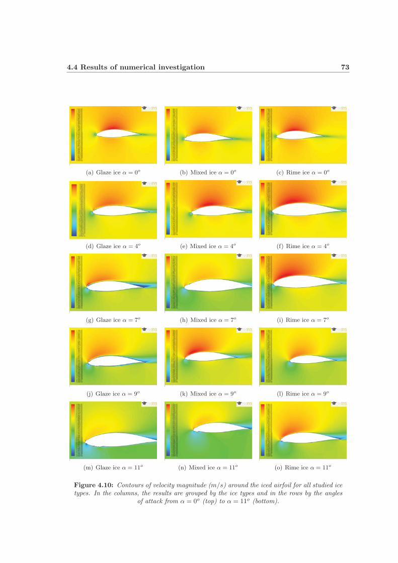
4.4 Results of numerical investigation 73
(a) Glaze ice α = 0o (b) Mixed ice α = 0o (c) Rime ice α = 0o
(d) Glaze ice α = 4o (e) Mixed ice α = 4o (f) Rime ice α = 4o
(g) Glaze ice α = 7o (h) Mixed ice α = 7o (i) Rime ice α = 7o
(j) Glaze ice α = 9o (k) Mixed ice α = 9o (l) Rime ice α = 9o
(m) Glaze ice α = 11o (n) Mixed ice α = 11o (o) Rime ice α = 11o
Figure 4.10: Contours of velocity magnitude (m/s) around the iced airfoil for all studied icetypes. In the columns, the results are grouped by the ice types and in the rows by the angles
of attack from α = 0o (top) to α = 11o (bottom).
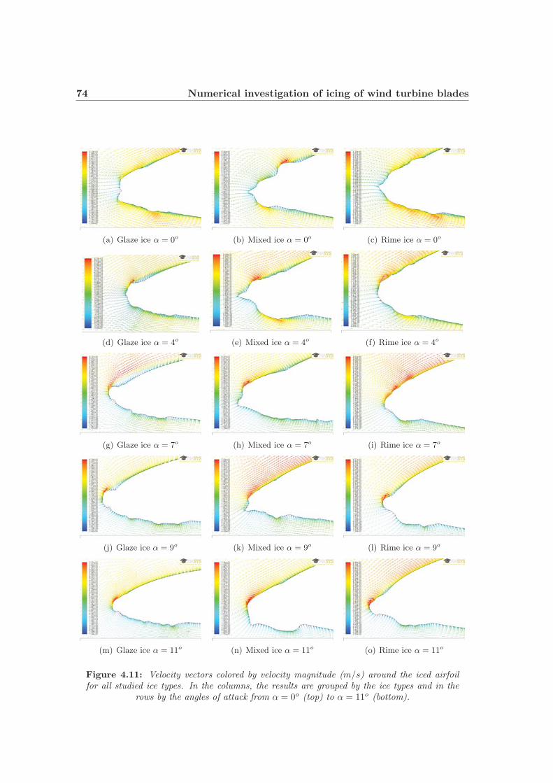
74 Numerical investigation of icing of wind turbine blades
(a) Glaze ice α = 0o (b) Mixed ice α = 0o (c) Rime ice α = 0o
(d) Glaze ice α = 4o (e) Mixed ice α = 4o (f) Rime ice α = 4o
(g) Glaze ice α = 7o (h) Mixed ice α = 7o (i) Rime ice α = 7o
(j) Glaze ice α = 9o (k) Mixed ice α = 9o (l) Rime ice α = 9o
(m) Glaze ice α = 11o (n) Mixed ice α = 11o (o) Rime ice α = 11o
Figure 4.11: Velocity vectors colored by velocity magnitude (m/s) around the iced airfoilfor all studied ice types. In the columns, the results are grouped by the ice types and in the
rows by the angles of attack from α = 0o (top) to α = 11o (bottom).
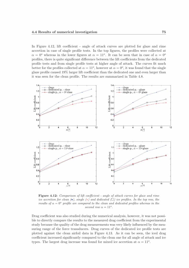
4.4 Results of numerical investigation 75
In Figure 4.12, lift coefficient - angle of attack curves are plotted for glaze and rimeaccretion in case of single profile tests. In the top figures, the profiles were collected atα = 0o whereas in the lower figures at α = 11o. It can be seen that in case of α = 0o
profiles, there is quite significant difference between the lift coefficients from the dedicatedprofile tests and from single profile tests at higher angle of attack. The curves fit muchbetter for the profiles collected at α = 11o, however at α = 0o, it was found that the singleglaze profile caused 19% larger lift coefficient than the dedicated one and even larger thanit was seen for the clean profile. The results are summarized in Table 4.8.
Figure 4.12: Comparison of lift coefficient - angle of attack curves for glaze and rimeice accretion for clean (•), single (∗) and dedicated (�) ice profiles. In the top row, theresults of α = 0o profile are compared to the clean and dedicated profiles whereas in the
second row α = 11o.
Drag coefficient was also studied during the numerical analysis, however, it was not possi-ble to directly compare the results to the measured drag coefficient from the experimentalstudy because the quality of the drag measurements was very likely influenced by the mea-suring range of the force transducers. Drag curves of the dedicated ice profile tests areplotted against the clean airfoil data in Figure 4.13. As it can be seen, the iced dragcoefficient increased significantly compared to the clean one for all angle of attack and icetypes. The largest drag increase was found for mixed ice accretion at α = 11o.
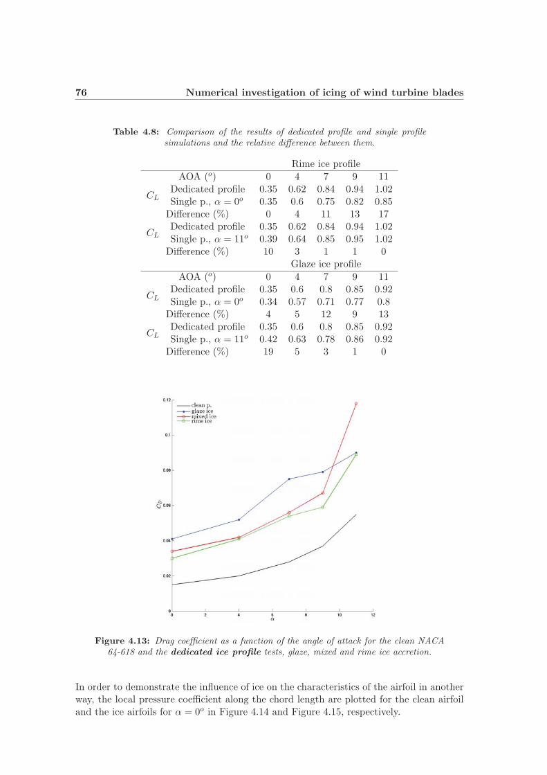
76 Numerical investigation of icing of wind turbine blades
Table 4.8: Comparison of the results of dedicated profile and single profilesimulations and the relative difference between them.
Rime ice profile
AOA (o) 0 4 7 9 11
CLDedicated profile 0.35 0.62 0.84 0.94 1.02Single p., α = 0o 0.35 0.6 0.75 0.82 0.85Difference (%) 0 4 11 13 17
CLDedicated profile 0.35 0.62 0.84 0.94 1.02Single p., α = 11o 0.39 0.64 0.85 0.95 1.02Difference (%) 10 3 1 1 0
Glaze ice profile
AOA (o) 0 4 7 9 11
CLDedicated profile 0.35 0.6 0.8 0.85 0.92Single p., α = 0o 0.34 0.57 0.71 0.77 0.8Difference (%) 4 5 12 9 13
CLDedicated profile 0.35 0.6 0.8 0.85 0.92Single p., α = 11o 0.42 0.63 0.78 0.86 0.92Difference (%) 19 5 3 1 0
Figure 4.13: Drag coefficient as a function of the angle of attack for the clean NACA64-618 and the dedicated ice profile tests, glaze, mixed and rime ice accretion.
In order to demonstrate the influence of ice on the characteristics of the airfoil in anotherway, the local pressure coefficient along the chord length are plotted for the clean airfoiland the ice airfoils for α = 0o in Figure 4.14 and Figure 4.15, respectively.
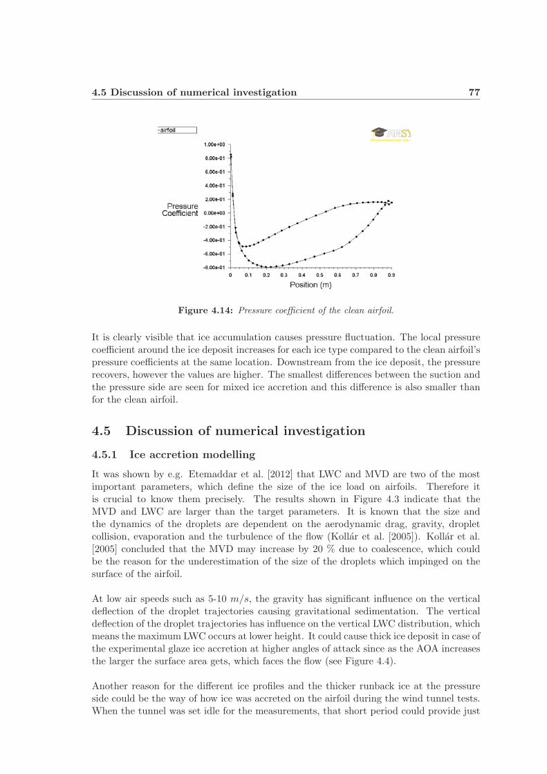
4.5 Discussion of numerical investigation 77
Figure 4.14: Pressure coefficient of the clean airfoil.
It is clearly visible that ice accumulation causes pressure fluctuation. The local pressurecoefficient around the ice deposit increases for each ice type compared to the clean airfoil’spressure coefficients at the same location. Downstream from the ice deposit, the pressurerecovers, however the values are higher. The smallest differences between the suction andthe pressure side are seen for mixed ice accretion and this difference is also smaller thanfor the clean airfoil.
4.5 Discussion of numerical investigation
4.5.1 Ice accretion modelling
It was shown by e.g. Etemaddar et al. [2012] that LWC and MVD are two of the mostimportant parameters, which define the size of the ice load on airfoils. Therefore itis crucial to know them precisely. The results shown in Figure 4.3 indicate that theMVD and LWC are larger than the target parameters. It is known that the size andthe dynamics of the droplets are dependent on the aerodynamic drag, gravity, dropletcollision, evaporation and the turbulence of the flow (Kollar et al. [2005]). Kollar et al.[2005] concluded that the MVD may increase by 20 % due to coalescence, which couldbe the reason for the underestimation of the size of the droplets which impinged on thesurface of the airfoil.
At low air speeds such as 5-10 m/s, the gravity has significant influence on the verticaldeflection of the droplet trajectories causing gravitational sedimentation. The verticaldeflection of the droplet trajectories has influence on the vertical LWC distribution, whichmeans the maximum LWC occurs at lower height. It could cause thick ice deposit in case ofthe experimental glaze ice accretion at higher angles of attack since as the AOA increasesthe larger the surface area gets, which faces the flow (see Figure 4.4).
Another reason for the different ice profiles and the thicker runback ice at the pressureside could be the way of how ice was accreted on the airfoil during the wind tunnel tests.When the tunnel was set idle for the measurements, that short period could provide just
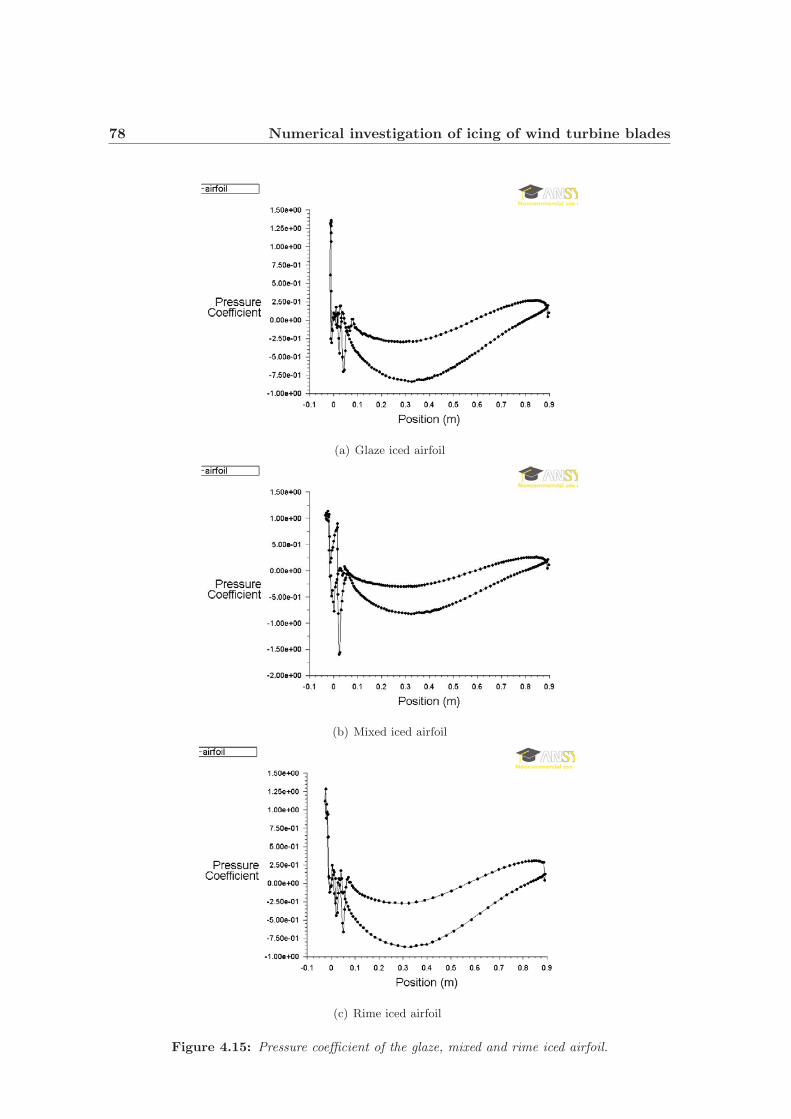
78 Numerical investigation of icing of wind turbine blades
(a) Glaze iced airfoil
(b) Mixed iced airfoil
(c) Rime iced airfoil
Figure 4.15: Pressure coefficient of the glaze, mixed and rime iced airfoil.

4.5 Discussion of numerical investigation 79
enough time for the water layer to freeze and hence the collided water droplets could notcompletely ran back or bounce off the airfoil.
This indicates that the development of the ice profiles was influenced by the combinationof the applied low wind seed, and thus coalescence and vertical deflection of the droplettrajectories, and the characteristics of the wind tunnel tests.
Additional simulations suggest that in case of rime ice profiles, the numerical profilesagree well with the experimental ones, if LWC is increased to 1g/m3 and the MVD to40μm.
4.5.2 Computational fluid dynamics
The roughness sensitivity tests showed that changing the roughness height and thus thefirst layer height of the mesh does not have a significant influence on the aerodynamicsbut has detrimental effect on the flow simulation in the vicinity of the iced airfoil profile.Therefore micro surface roughness was neglected during the simulations.
The trend of the lift coefficient - angle of attack curves from the numerical analyses are ingood agreement with the ones from the wind tunnel tests, as shown in Figure 4.5. How-ever, the values from the wind tunnel are much lower than the ones from the numericalsimulations due to the fact that the measurements were only corrected for lift interfer-ence and blockage interference but not for the presence of the vertical walls. Based onthe numerical results of the clean airfoil studies, it was found that the vertical walls hadstrong impact on the measurements and the effective chord width was reduced by 20%. The immediate effect of the vertical wall on the flow behaviour is also visible on theflow visualisation photos from LM Wind Power presented in Figure 3.11 in the previouschapter.
After correcting the experimental results, still quite large differences were found. A reasonfor these differences could be that with the contour tracing method, the small changesof surface roughness could not be documented therefore they were not implemented inthe numerical analysis. It was shown in many studies (e.g. Bragg et al. [2005]) thatthe roughness highly affects the aerodynamics of the airfoil. Based on the differencesin the aerodynamic effect between 2 D and 3D ice shapes, Addy [2000] concluded thatthe surface roughness and the irregularities present in natural aircraft ice are importantcharacteristics. The CFD models were 2-D, and thus it was impossible to properly im-plement the highly 3-D structure of the ice deposit, which was seen for example in Figure3.18 or in Figure 3.26. It can be seen that the beads and feathers are very complex andrough, and probably it would be quite challenging to properly model them even in 3-D.These could also cause the differences between the results of the wind tunnel tests andthe numerical simulations.
The measured relative reduction of lift coefficient (listed in Table 4.6) shows also quitelarge difference from the ones listed in Table 4.7, which implies that the combination ofthe presence of the wind tunnel’s vertical walls and the changed surface roughness hadsignificant influence on the measurements. For lower angles of attack, especially α = 0o,
80 Numerical investigation of icing of wind turbine blades
the difference between the measured and simulated relative reduction is significantly large,which indicates that the altered surface roughness had the highest influence on the liftreduction.
Similarly to e.g. Homola et al. [2010a], lift was found to decrease in all cases. E.g. Virket al. [2010b] found higher lift coefficients for rime iced profiles than for the clean profilesdue to the increased effective chord length and camber of the blade profile. This wasnot experienced in the presented cases of dedicated profile simulations. However, as itcan be seen in Figure 4.11, the curvature of the ice shapes follows well the curve of theairfoil at the suction side, i.e. acts as an extended leading edge, and thus could cause lesssignificant lift degradation than e.g. the glaze ice accretion.
A tendency of increased lift reduction was seen for glaze ice accretion as the AOA in-creased. This is due to the characteristics of glaze ice. During glaze ice accretion, becauseof the relatively higher air temperature (0 −− 4oC), not all water droplets freeze to thesurface on impact and hence some run along the airfoil and freeze later (Bose [1992]).As AOA increases, the area exposed to the water droplets increases as well, therefore itcauses more flow disturbance and thus more lift reduction.
In most cases, mixed ice accretion caused more significant lift degradation than glaze iceaccretion due to the large ice deposit, which accumulated on the leading edge and hencecaused higher flow disturbance (see Figure 4.11).
A significant change in the flow pattern was observed, when a comparison was madebetween flow around the clean and the iced blade profiles due to the changes of the aero-dynamically shaped leading edge curve. As AOA was increased, the surface area, whichfaced the incoming flow and thus the water droplets, increased as well causing majorchanges in the local flow pattern.
In Figure 4.11, small local separations are seen, which were also reported in the study ofReid et al. [2013]. In these set of figures, it can be noticed that the suction effect wasreduced at the suction side (which was also reported by Villalpando et al. [2012]) and ledto lift reduction.
The impact of single ice profiles collected at α = 0o and α = 11o were studied at differentangles of attack. The lift coefficients of α = 0o for both glaze and rime ice accretion arelower than the ones found in case of dedicated profile tests. The reason for this differencecould be that ice was accumulated only on the leading edge in case of α = 0o and whenthe incident angle of incoming flow is increased, the stagnation point moves downstreamof the ice deposit disturbing the flow on the suction side, which has higher influence onthe lift coefficient than the pressure side. The profiles collected at α = 11o did not causesignificantly different lift curves from the multiple profiles because for α < 11o values, theice deposit is downstream of the stagnation point.
Drag coefficient was also studied during the numerical analysis for U = 25m/s. As it wasexpected the drag coefficient increased compared to the clean airfoil for each AOA andice type. The curves in Figure 4.13 are not smooth and it is not possible to fit any poly-
4.6 Conclusion drawn from the numerical investigation 81
nomial to the point either. The reason is the differently iced profiles, which have differentinfluence on the flow field and thus on the aerodynamics. The largest drag increase wasfound for mixed ice tests, since the large ice deposit accreted for mixed ice condition andthe flow was disturbed the most significantly. It was seen that for lower AOA, the dragcoefficient of the iced airfoils was smaller than of the clean profile.
Around the ice deposit, the local pressure coefficient increased and is fluctuating due tothe rather rough and complex surface. Downstream of the ice, the pressured coefficientcurves became smooth again.
4.6 Conclusion drawn from the numerical investigation
In this chapter, the collected ice profiles were numerically studied in order to validatethe settings of the wind tunnel and the profiles and also to analyse the impacts of iceaccretion on the flow conditions around the iced airfoil and the lift coefficient.
The TURBICE simulations showed that the values of the median volume diameter andliquid water content were underestimated. The resulted MVD and LWC were larger thanthe target values for rime ice accretion. The results of TURBICE simulation also indicatethat the development of the ice profiles was influenced by the combination of the appliedlow wind seed, and thus coalescence and vertical deflection of the droplet trajectories,and the characteristics of the wind tunnel tests.
The results of the Ansys Fluent analyses imply that the combination of the presence ofthe vertical wall of the wind tunnel and the changed surface roughness had significantinfluence on the measurements. However, the trend of the lift coefficient - angle of attackcurves from the numerical analyses are in good agreement with the ones from the windtunnel tests. Comparing the measured lift coefficient to the computational ones, it wasfound that the effective span was approximately 80% of the geometric span due to thepresence of the end plates. Based on this information, the measured lift coefficients werecorrected.
Quite large differences between the measured relative lift reductions and the numericalones were observed, because the surface roughness was not possible to be implementedin the CFD simulation. A significant change in the flow pattern was observed, when acomparison was made between clean and iced blade profiles due to the changes of theaerodynamically shaped leading edge curve. The sharp edges at the suction side of glazeand mixed ice profiles led to a speed up, which caused a large separation bubble. In caseof rime iced profile, the flow followed a similar pattern as it was observed for the cleanairfoil and the magnitude of the velocity did not differ significantly from the clean profile.For all three cases, there were some vortex formations noticed behind the ice peaks atthe pressure side causing tiny recirculation zones, which led to some flow disturbance andretardation. However, they did not have a large influence on the change of the overallleading edge aerodynamics. The experiments also showed a clear 3-D ice pattern thatrequires 3-D computations.
As it was expected, the drag coefficient increased due to the ice accretion for all ice types.

82 Numerical investigation of icing of wind turbine blades
The largest increase was experienced in case of mixed ice for α = 11o. It was also seenthat the ice deposit caused pressure fluctuation, and the pressure coefficient increased foreach ice type for the shown α = 0o cases.
The importance of the angle of attack, on which the profiles were collected, on the liftcoefficient was shown. The results of the single profile tests in case of α = 0o for both glazeand rime ice accretion gave lower lift coefficients than the ones for dedicated profile tests.The reason for this difference could be that ice was accumulated only on the leading edgein case of α = 0o and when the incident angle of incoming flow increased, the stagnationpoint moved downstream from the ice deposit on the suction side.

Chapter 5
Transformation of lift coefficients
Seifert and Richert [1997] introduced a transformation method with which they claimedit was possible to transform measured aerodynamic coefficients from an iced airfoil to anyother airfoils. In that work, the measured iced NACA 4415 profile was used to transforme.g. the lift coefficient to a NACA 63-415 airfoil. In Figure 5.1, the method of how tointerpolate the iced coefficients of an airfoil is shown. NACA denotes the measured airfoilwhereas NP refers to the ”new profile”.
Figure 5.1: Method to interpolate the iced coefficients of the airfoil (Seifert and Richert[1997]). NACA denotes the measured airfoil whereas NP the ”new profile”.
The aim of this study was to see whether it had been possible to transform the liftcoefficients of the measured iced NACA 4415 to the NACA 64-618, which was used inthis PhD work. The results were then compared to the results of the wind tunnel testsand also of the numerical simulations. Only the rime iced airfoil’s results are used becausethat type of ice was studied by Seifert and Richert [1997] as well.
The method is rather poorly explained in the reference, therefore first, it was necessary toreproduce the published results for the NACA 63-415. The following routine was followed:
�CcleanL = Cclean
L,NACA − CcleanL,NP (5.1)
CicedL,NP = Ciced
L,NACA −�CcleanL ∗Ka (5.2)
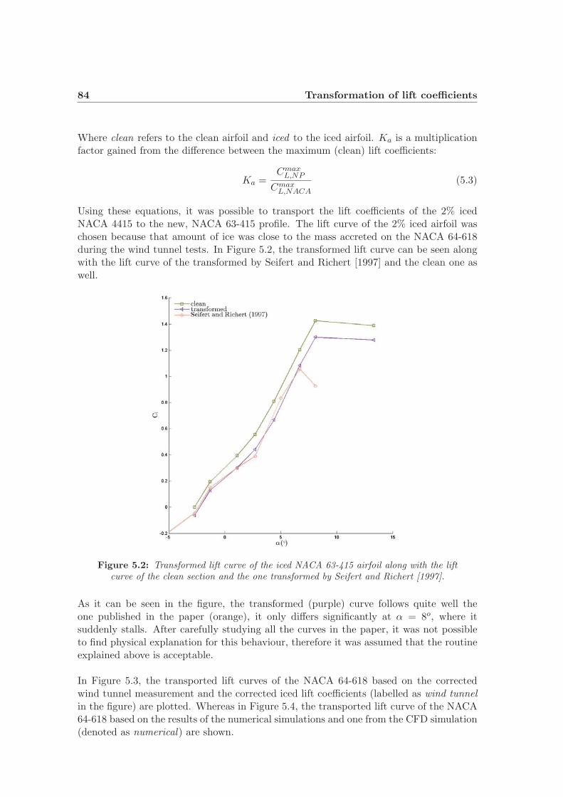
84 Transformation of lift coefficients
Where clean refers to the clean airfoil and iced to the iced airfoil. Ka is a multiplicationfactor gained from the difference between the maximum (clean) lift coefficients:
Ka =CmaxL,NP
CmaxL,NACA
(5.3)
Using these equations, it was possible to transport the lift coefficients of the 2% icedNACA 4415 to the new, NACA 63-415 profile. The lift curve of the 2% iced airfoil waschosen because that amount of ice was close to the mass accreted on the NACA 64-618during the wind tunnel tests. In Figure 5.2, the transformed lift curve can be seen alongwith the lift curve of the transformed by Seifert and Richert [1997] and the clean one aswell.
Figure 5.2: Transformed lift curve of the iced NACA 63-415 airfoil along with the liftcurve of the clean section and the one transformed by Seifert and Richert [1997].
As it can be seen in the figure, the transformed (purple) curve follows quite well theone published in the paper (orange), it only differs significantly at α = 8o, where itsuddenly stalls. After carefully studying all the curves in the paper, it was not possibleto find physical explanation for this behaviour, therefore it was assumed that the routineexplained above is acceptable.
In Figure 5.3, the transported lift curves of the NACA 64-618 based on the correctedwind tunnel measurement and the corrected iced lift coefficients (labelled as wind tunnelin the figure) are plotted. Whereas in Figure 5.4, the transported lift curve of the NACA64-618 based on the results of the numerical simulations and one from the CFD simulation(denoted as numerical) are shown.
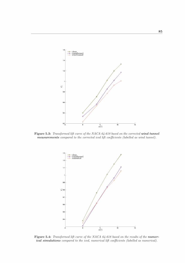
85
Figure 5.3: Transformed lift curve of the NACA 64-618 based on the corrected wind tunnelmeasurements compared to the corrected iced lift coefficients (labelled as wind tunnel).
Figure 5.4: Transformed lift curve of the NACA 64-618 based on the results of the numer-ical simulations compared to the iced, numerical lift coefficients (labelled as numerical).

86 Transformation of lift coefficients
Comparing Figure 5.3 and Figure 5.4, it can be seen that the transformed lift curve fitsmuch better to the one from the CFD analysis. A reason could be that the 2 % ice masswas different from the one collected during the wind tunnel tests or that the method doesnot include the change of the surface roughness as it was not included in the numericalanalysis either. Another reason for the difference between the lift curve from the windtunnel tests and the transformed one could be that it is unknown at which AOA thetested ice fragment was collected. The importance of this information was shown inSection 4.4.2.
Although only one independent scenario was demonstrated for the usability of the methodof Seifert and Richert [1997], the results are promising. It is suspected that it could be astrong basis of a very useful aerodynamic coefficient transformation model.

Chapter 6
Conclusion drawn from the PhDwork
The PhD study was carried out at the Department of Wind Energy, Technical Universityof Denmark. The work can be divided into two larger parts. In the first part, the influ-ence of environmental and meteorological parameters on the occurrence of icing eventswas studied on a specific case in South-Greenland. In the larger, second part, experi-mental and numerical investigations of the impact of ice accretion on wind turbine bladeswere carried out.
During the risk analysis of icing in South-Greenland, different direct and indirect tech-niques, which can identify probable icing periods, were studied. Similarly to other studies,it was experienced that none of the methods can identify icing events certainly on its own.However, combining the different techniques, a quite good picture of these events can beobtained. The best performing technique was found to be the comparison of the outputof heated and unheated anemometers.
Dedicated ice rate sensor from HoloOptics was also tested in two locations in South-Greenland. Despite of the expectations, the instrument could not provide data for thewhole length of the measurement campaign because due to unknown reasons (might bevoltage outage or lightening), all three, independently installed instruments broke duringwinter. However when they were functional, they could provide useful information notonly about the extent of the icing event but also about its severity.
The data analysis indicates that icing events usually occur during periods with low windspeed, high relative humidity and subzero (or close to 0 o) temperature especially duringnight or cloudy/foggy periods. The same observation was reported by the research groupat Summit Station. It can be concluded that icing might be a significant issue in SouthGreenland, but a more thorough and dedicated, location dependent investigation is nec-essary when the decision is made to install wind turbines in a specific location.
Wind tunnel tests were performed on a NACA 64-618 airfoil at the Collaborative ClimaticWind Tunnel. During the experimental work, glaze, rime, and mixed ice accretions werestudied and the changes of aerodynamic forces and the accreted mass were monitored asice was building up on the blade. Both processes were found to be nearly linear. Theimmediate alteration of the surface roughness was experienced to have more significantdetrimental effect on the lift coefficient than the shape of the changed airfoil in that very
88 Conclusion drawn from the PhD work
early stage of ice accretion. With increasing angle of attack the degradation of the instan-taneous lift coefficient increases as well. The most significant lift coefficient degradationwas seen in case of mixed ice accretion. The largest ice mass also accumulated for that icetype and caused high flow disturbance, which could then lead to the high lift reduction.
The results of the experimental investigation showed that the type of the ice accretionhas significant impact on the degree of the reduction of the lift coefficient and thus on thepower production loss. Independently of the ice type, ice accumulation has strong nega-tive influence on the flow field around the airfoil, which was also confirmed by both theflow visualization and the numerical analysis. It was also observed that the ice accretion ishighly 3-D. In case of glaze ice accretion, small ice bead formation was observed whereasin case of mixed ice accretion, a sharp nose-like ice peak formed around the stagnationpoint. These could occur, because the airfoil was static during the tests and also becausethe wind tunnel was set to idle every 5 minutes for measurement for couple of minutes,which was long enough time to freeze all the already impinged liquid water droplets.
The mass and the shape of the ice deposit are highly dependent on LWC, MVD andtemperature. It also has to be underlined that the accreted mass was smaller than itwould have accumulated on the blade of an operating wind turbine due to the relativelylow wind speed that was applied in the wind tunnel in order to ensure low enough airtemperature.
The increase of the drag coefficient was also nearly linear process, however due to thewide measuring range of the force transducers, the presented values are probably toohigh. A brief analysis of the melting process was also done. It was observed that aslong as the air temperature remained subzero inside the tunnel, no ice melting happened,which implies the sun is probably the most important element of the melting process atlow temperature. As air temperature increased above freezing point, a thin melt waterlayer appeared between the ice and the airfoil, which most likely helps the ice deposit toshed off from a rotating wind turbine blade.
At the end of each wind tunnel test, the shape of the ice deposit was recorded by con-tour tracing method. These profiles were then used during the numerical investigation.Dedicated computational ice accretion model, TURBICE from VTT, Technical ResearchCentre of Finland was used to calibrate the environmental parameters for MVD and LWC.The simulations showed that these values were underestimated in the wind tunnel. MVDwas larger due to coalescence of the incoming droplets, which then impinged on the sur-face of the airfoil. The vertical deflection of the droplet trajectories had influence on thevertical LWC distribution, i.e. the maximum LWC occurred at lower height. The com-bined effect of these two phenomena could also lead to formation of a larger ice deposit atthe pressure side of the airfoil. Additional simulations suggested that the best fits are forall angles of attack for rime ice accretion with LWC � 1g/m3 and MVD � 40μm andrather than 0.6 g/m3 and 23μm, as specified by the manufacturer of the spray nozzlesbased on the setted water and air pressure.
Simulations with Ansys Fluent were then performed to quantify the impacts of ice accre-tion on the flow behaviour and the aerodynamic characteristics of the iced airfoil from the

89
wind tunnel tests. Comparison was made between the lift coefficients of the clean profilefrom the numerical analysis and the ones from the wind tunnel tests, which implied thatthe presence of the vertical walls had significant influence on the measurements. It wasfound that the effective span was 20% shorter than the geometric one. After correctingthe wind tunnel measurements, there were still quite significant differences found. Thereason could be the micro surface roughness of the ice deposit, which was not implementedin the numerical model due to the experience that Fluent cannot properly handle it. Theother explanation could be the strong 3-D characteristics of the ice deposit (beads andfeathers), which cannot be properly modelled in 2-D, but have significant influence on theflow.
Although the drag coefficients could not be directly compared to the results of the windtunnel tests, the drag curves were studied. It was seen that the drag increases significantlyfor all ice types. The largest increase was found at α = 11o for mixed ice.
A significant change in the flow pattern was observed for all cases and the most significantflow disturbance was caused by mixed ice accretion. For all three ice types, there weresome vortex formations noticed behind the ice peaks at the pressure side, which causedtiny recirculation zones and led to minor flow disturbance. However, they did not havea large influence on the change of the overall leading edge aerodynamics. At the suctionside, especially for glaze ice, small ice peaks formed, which caused local speed-up at theirsharp edges. Behind these peaks recirculation zones could develop. The most significantflow disturbance and also the largest number of recirculation zones formed in case of glazeand mixed ice, which led to the highest lift coefficient reductions as well.
It was shown that the lift coefficients are highly dependent on the angle of attack onwhich the profiles were collected. The impact of single ice profiles collected at α = 0o
and α = 11o were studied in flows with different incident angles. The lift coefficients ofα = 0o for both glaze and rime ice accretion were lower than the ones found in case ofdedicated profile tests.
Furthermore, it can be concluded that even one hour of ice accretion can significantlyreduce the lift coefficient of an airfoil and that the angle of attack at which the ice buildsup on the surface is highly important.
The final lift curves of rime ice accretion from both experimental and numerical investi-gation were used in a demonstration of the transformation model of Seifert and Richert[1997]. It was found that the transformed lift curve fits much better to the one from theCFD analysis. The reason could be either that the method does not include the changeof the surface roughness therefore the transformed lift curve could fit to the numericalone or because it is unknown at which AOA the tested ice fragment was collected andthe importance of this information was clearly shown during the numerical investigation.However, it can be concluded that the usability of the method of Seifert and Richert [1997]is promising and it could probably provide a strong basis for a very useful aerodynamiccoefficient transformation model.

90 Conclusion drawn from the PhD work

Chapter 7
Future work
Although during the three years of PhD study, several topics related to icing of windturbine blades were investigated, the findings have raised a number of questions and havegiven ideas for further improvements, studies and researches. In this chapter some ofthese suggestions are listed.
Experimental investigation
� There is a desperate need for standardize MVD and LWC techniques especially sinceit was shown several times that these two are of the most important parameters.
� Drag force measurements with heated measurement system or a more suitable forcebalance (with smaller measurement range to be able to capture the very smallchanges as well) could give similar information on the changes as it was seen in caseof the list measurements.
� More wind tunnel tests with different LWC, MVD and AOA and different airfoilsections
� Employment of infra-red camera to study the surface temperature prior and alsoduring ice accretion could give useful information on the accretion process ans alsowould be essential for the melting investigation.
� Thorough surface roughness tests including ageing of airfoil surface. It was shownthat sand and insects are changing the surface roughness of the blades. So a studyof their impacts of ice accretion might be interesting.
� More detailed melting investigation would be interesting.
� Measurement of adhesion force of ice could be an additional feature.
Numerical investigation
� Proper surface roughness implementation is crucial for correct representation of thechanges of flow conditions due to ice accretion.
� Since in this study, only 2-D cases were modelled and it was seen that there mightbe significant differences in the aerodynamic effect between 2-D and 3-D ice shapes,therefore a detailed 3-D study is suggested.

92 Future work
� During the present work RANS turbulence models were used therefore it is suggestedto to test LES and DES models as well.

Appendix A
Risk of ice in South-Greenland forwind energy
In this Appendix chapter, the plots of the different ice detection methods, which weredetailed in Chapter 2, are shown.
A.1 Relative humidity and temperature
In total 112 hours of icing event in 16 days were identified with this method during thestudied 7 winter months.
Figure A.1: Number of daily icing hours based on RH and temperature measurementsduring winter months 2007-2008.
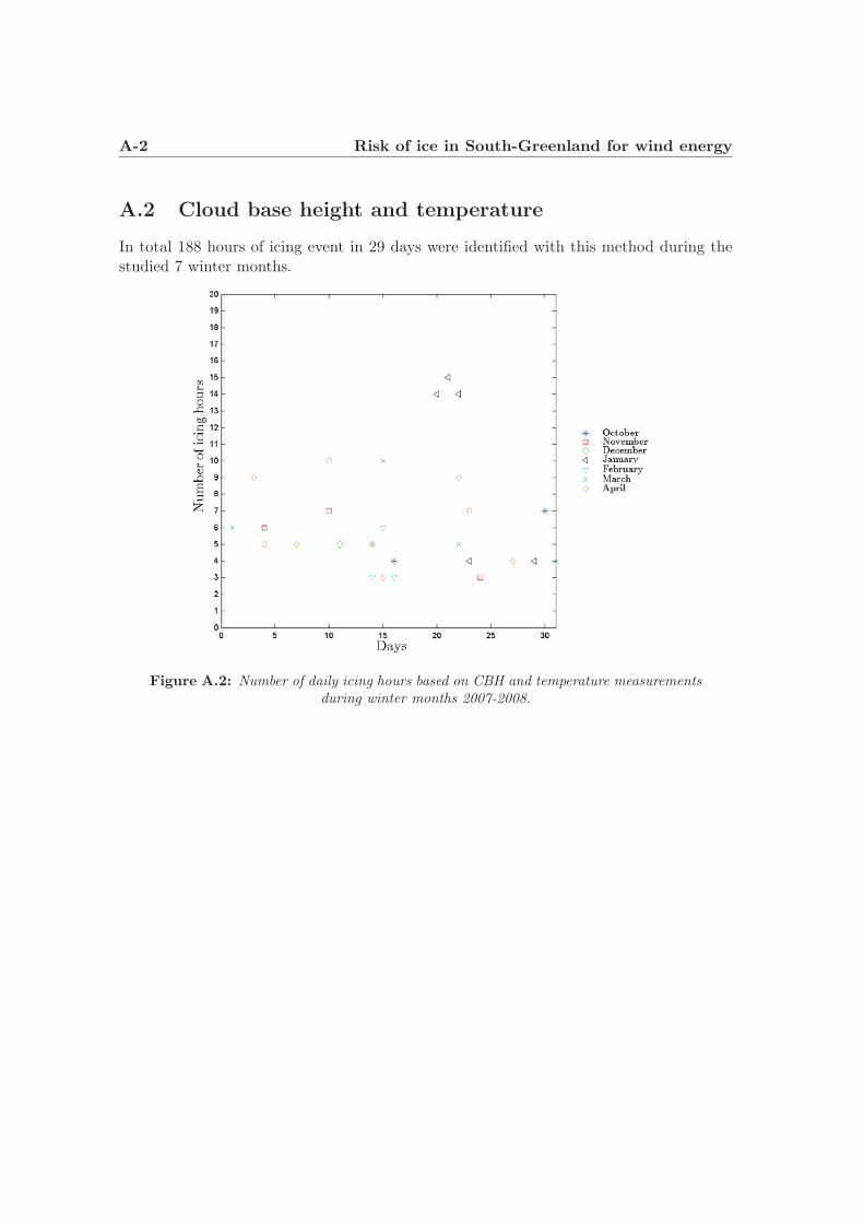
A-2 Risk of ice in South-Greenland for wind energy
A.2 Cloud base height and temperature
In total 188 hours of icing event in 29 days were identified with this method during thestudied 7 winter months.
Figure A.2: Number of daily icing hours based on CBH and temperature measurementsduring winter months 2007-2008.
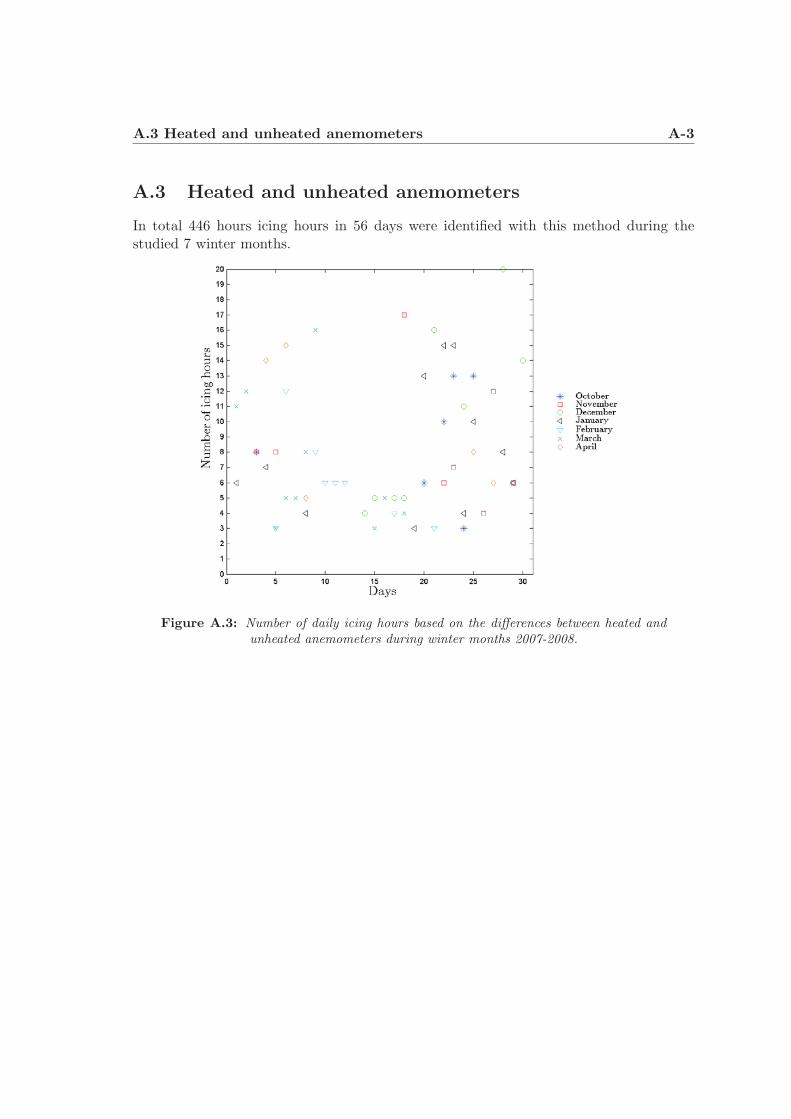
A.3 Heated and unheated anemometers A-3
A.3 Heated and unheated anemometers
In total 446 hours icing hours in 56 days were identified with this method during thestudied 7 winter months.
Figure A.3: Number of daily icing hours based on the differences between heated andunheated anemometers during winter months 2007-2008.
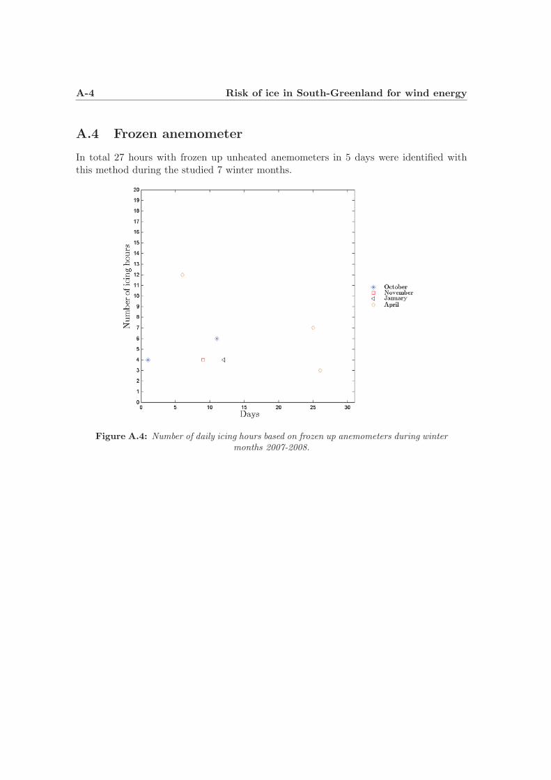
A-4 Risk of ice in South-Greenland for wind energy
A.4 Frozen anemometer
In total 27 hours with frozen up unheated anemometers in 5 days were identified withthis method during the studied 7 winter months.
Figure A.4: Number of daily icing hours based on frozen up anemometers during wintermonths 2007-2008.
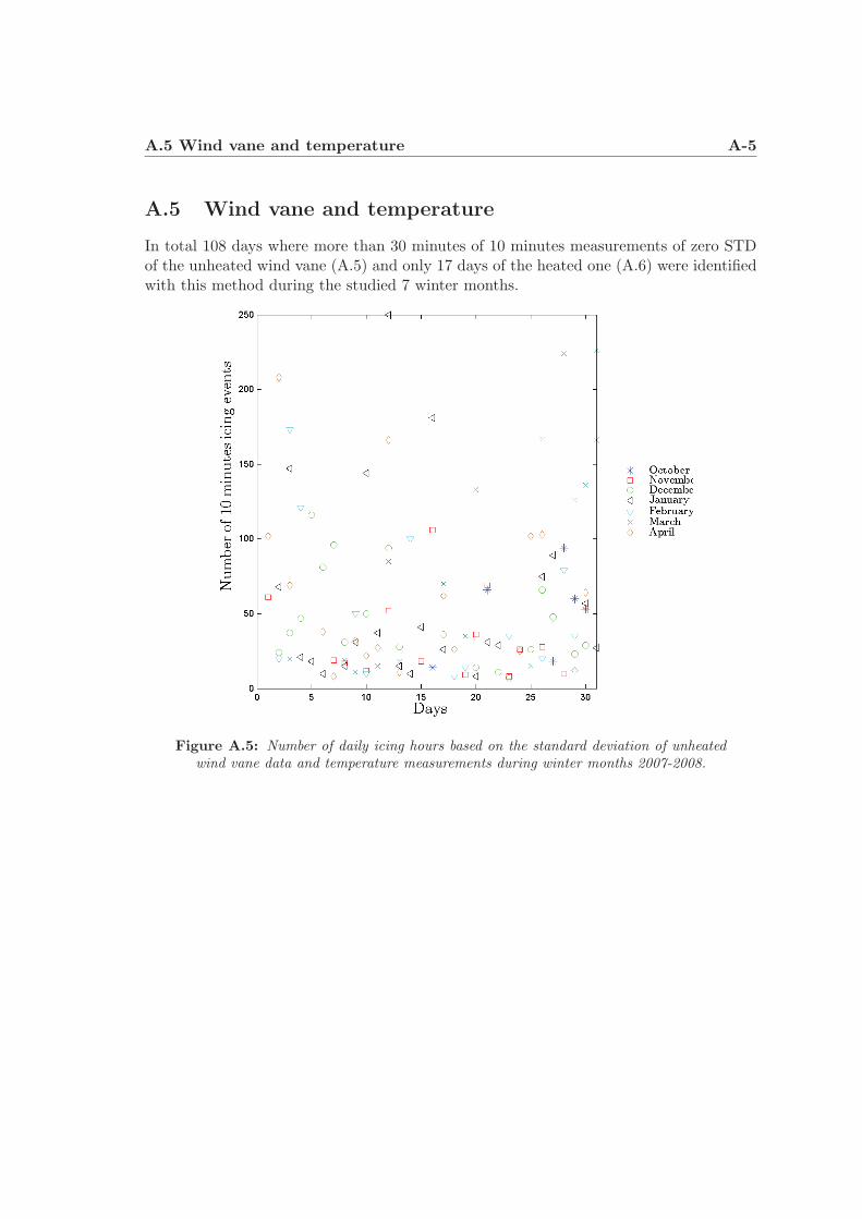
A.5 Wind vane and temperature A-5
A.5 Wind vane and temperature
In total 108 days where more than 30 minutes of 10 minutes measurements of zero STDof the unheated wind vane (A.5) and only 17 days of the heated one (A.6) were identifiedwith this method during the studied 7 winter months.
Figure A.5: Number of daily icing hours based on the standard deviation of unheatedwind vane data and temperature measurements during winter months 2007-2008.
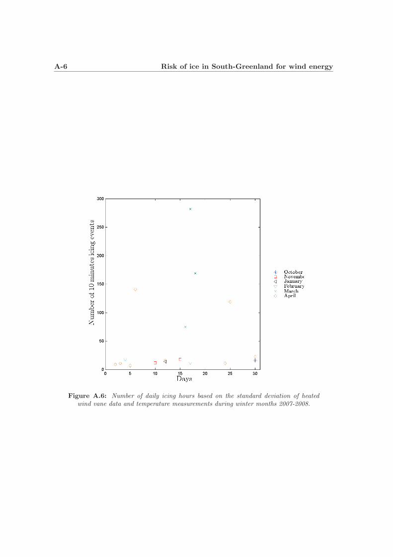
A-6 Risk of ice in South-Greenland for wind energy
Figure A.6: Number of daily icing hours based on the standard deviation of heatedwind vane data and temperature measurements during winter months 2007-2008.
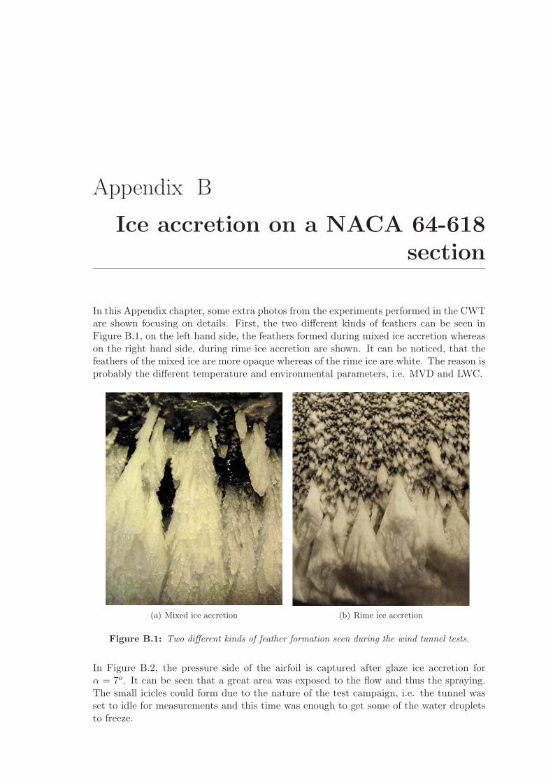
Appendix B
Ice accretion on a NACA 64-618section
In this Appendix chapter, some extra photos from the experiments performed in the CWTare shown focusing on details. First, the two different kinds of feathers can be seen inFigure B.1, on the left hand side, the feathers formed during mixed ice accretion whereason the right hand side, during rime ice accretion are shown. It can be noticed, that thefeathers of the mixed ice are more opaque whereas of the rime ice are white. The reason isprobably the different temperature and environmental parameters, i.e. MVD and LWC.
(a) Mixed ice accretion (b) Rime ice accretion
Figure B.1: Two different kinds of feather formation seen during the wind tunnel tests.
In Figure B.2, the pressure side of the airfoil is captured after glaze ice accretion forα = 7o. It can be seen that a great area was exposed to the flow and thus the spraying.The small icicles could form due to the nature of the test campaign, i.e. the tunnel wasset to idle for measurements and this time was enough to get some of the water dropletsto freeze.
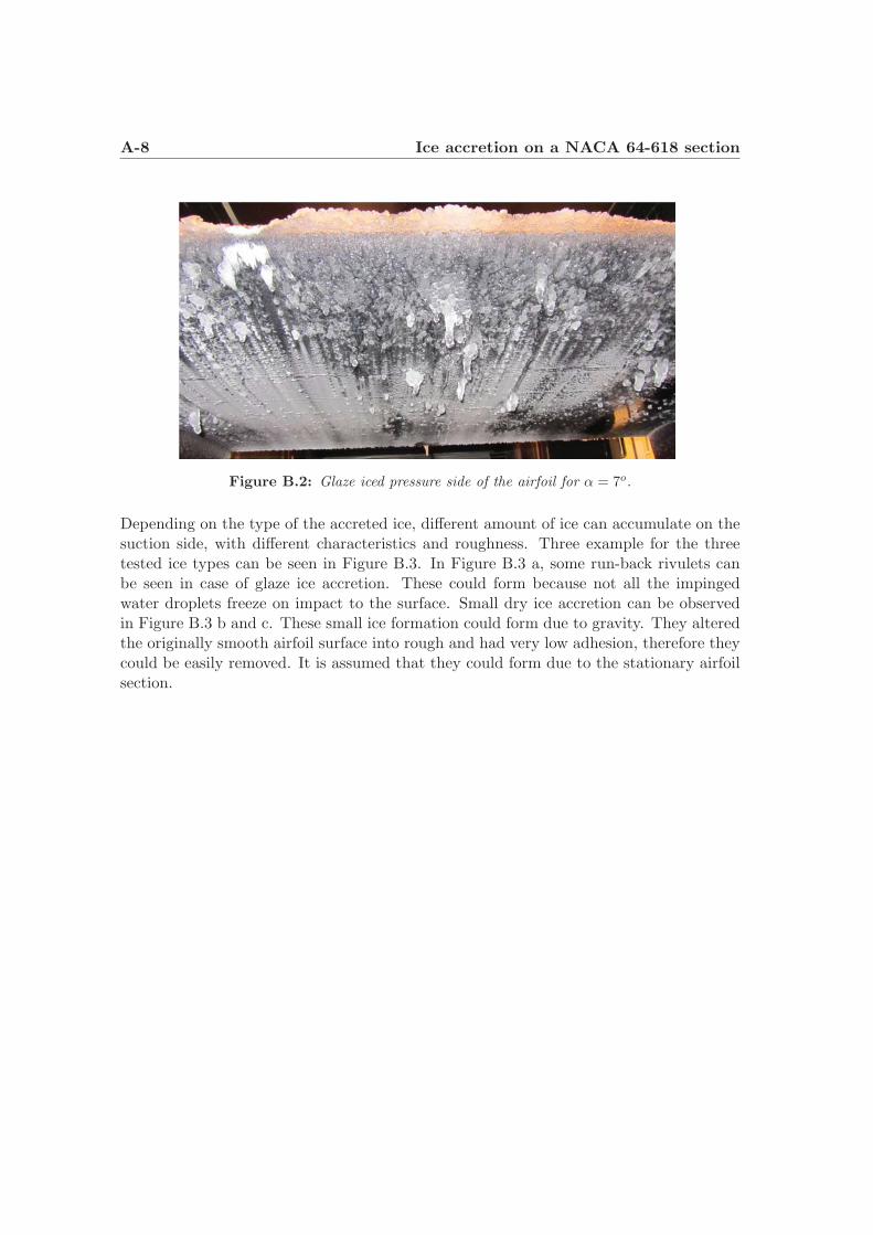
A-8 Ice accretion on a NACA 64-618 section
Figure B.2: Glaze iced pressure side of the airfoil for α = 7o.
Depending on the type of the accreted ice, different amount of ice can accumulate on thesuction side, with different characteristics and roughness. Three example for the threetested ice types can be seen in Figure B.3. In Figure B.3 a, some run-back rivulets canbe seen in case of glaze ice accretion. These could form because not all the impingedwater droplets freeze on impact to the surface. Small dry ice accretion can be observedin Figure B.3 b and c. These small ice formation could form due to gravity. They alteredthe originally smooth airfoil surface into rough and had very low adhesion, therefore theycould be easily removed. It is assumed that they could form due to the stationary airfoilsection.
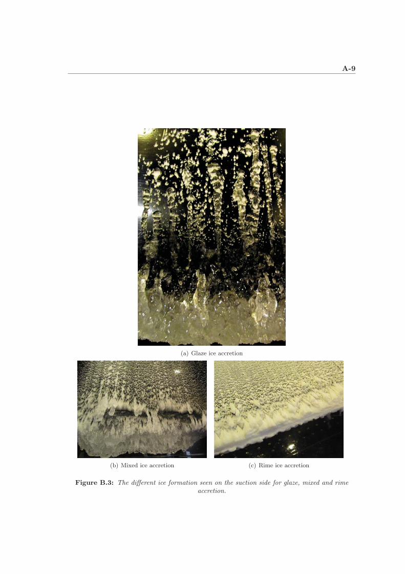
A-9
(a) Glaze ice accretion
(b) Mixed ice accretion (c) Rime ice accretion
Figure B.3: The different ice formation seen on the suction side for glaze, mixed and rimeaccretion.

A-10 Ice accretion on a NACA 64-618 section
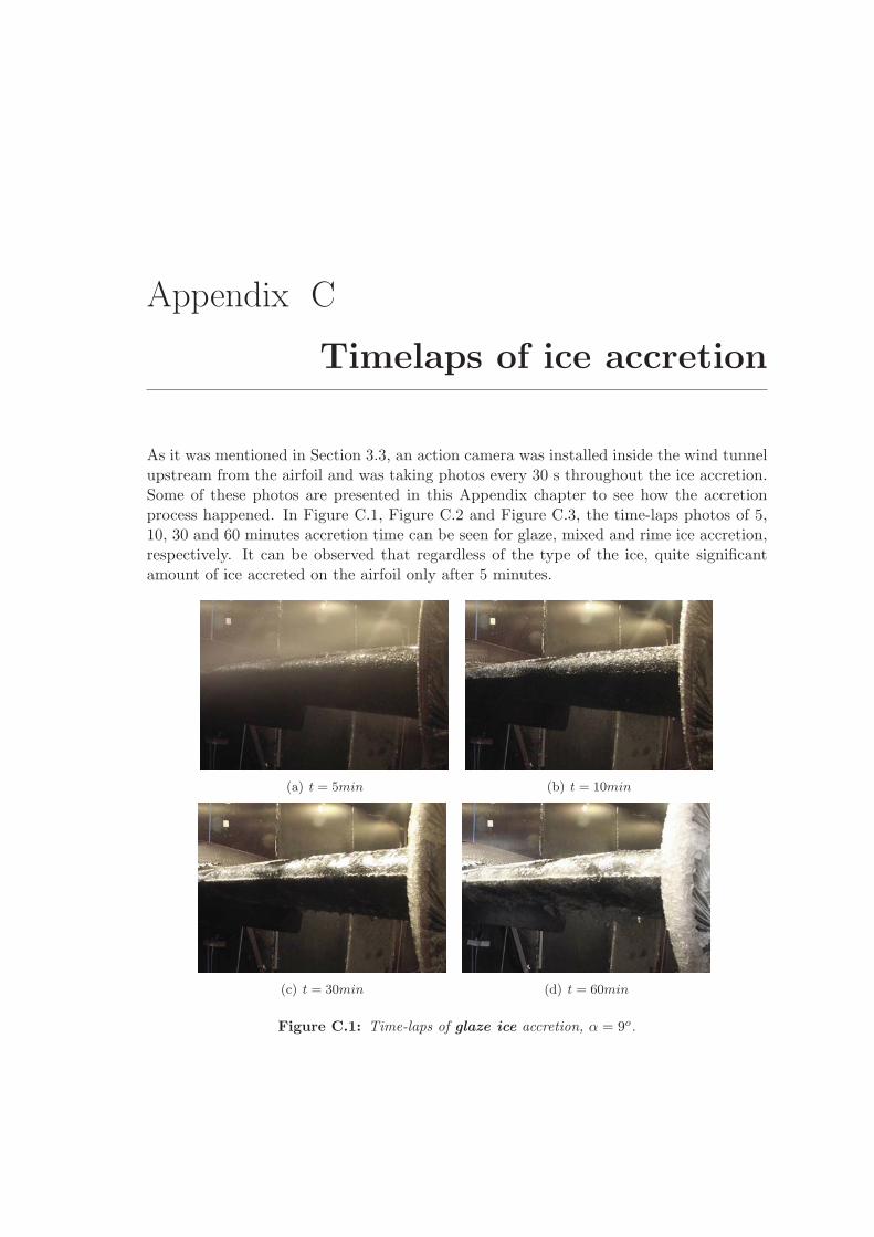
Appendix C
Timelaps of ice accretion
As it was mentioned in Section 3.3, an action camera was installed inside the wind tunnelupstream from the airfoil and was taking photos every 30 s throughout the ice accretion.Some of these photos are presented in this Appendix chapter to see how the accretionprocess happened. In Figure C.1, Figure C.2 and Figure C.3, the time-laps photos of 5,10, 30 and 60 minutes accretion time can be seen for glaze, mixed and rime ice accretion,respectively. It can be observed that regardless of the type of the ice, quite significantamount of ice accreted on the airfoil only after 5 minutes.
(a) t = 5min (b) t = 10min
(c) t = 30min (d) t = 60min
Figure C.1: Time-laps of glaze ice accretion, α = 9o.
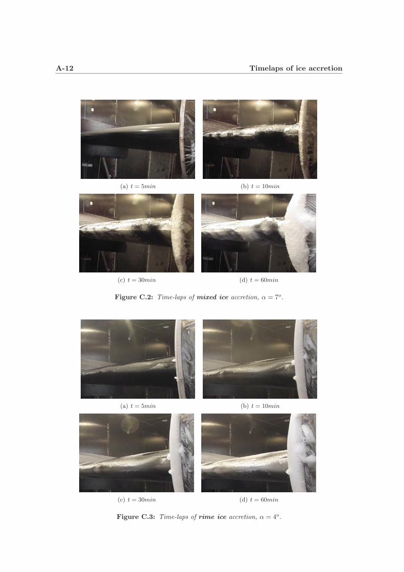
A-12 Timelaps of ice accretion
(a) t = 5min (b) t = 10min
(c) t = 30min (d) t = 60min
Figure C.2: Time-laps of mixed ice accretion, α = 7o.
(a) t = 5min (b) t = 10min
(c) t = 30min (d) t = 60min
Figure C.3: Time-laps of rime ice accretion, α = 4o.
Appendix D
TURBICE ice accretion model,results
In Section 4.4.1, the results of the computational ice accretion model, TURBICE aredetailed and some samples of the results are also shown there. In this Appendix chapter,the rest of the results are presented.
A direct comparison of the profiles from the wind tunnel to the ones from TURBICE areshown in Figure D.1 and Figure D.2. As it can be seen, setting the same environmentalparameters for LWC and MVD in TURBICE as the aimed ones from the wind tunneltests resulted in significantly smaller numerical ice profiles, which indicates that these twoparameters were highly underestimated.
Since the TURBICE simulations were done prior the final wind tunnel tests, it was nec-essary to produce as many scenarios as it was possible in order to have a catalogue to beable to properly verify the environmental parameters for LWC and MVD. Using the plotsin Figure D.3 and D.4, it gave valuable help for the range necessary for the additionalnumerical simulations. It could be concluded that LWC can be found in a range between0.8− 1g/m3 where as MVD is around 35− 40μm.
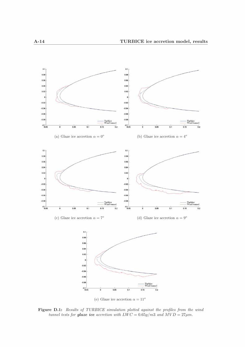
A-14 TURBICE ice accretion model, results
(a) Glaze ice accretion α = 0o (b) Glaze ice accretion α = 4o
(c) Glaze ice accretion α = 7o (d) Glaze ice accretion α = 9o
(e) Glaze ice accretion α = 11o
Figure D.1: Results of TURBICE simulation plotted against the profiles from the windtunnel tests for glaze ice accretion with LWC = 0.65g/m3 and MVD = 27μm.
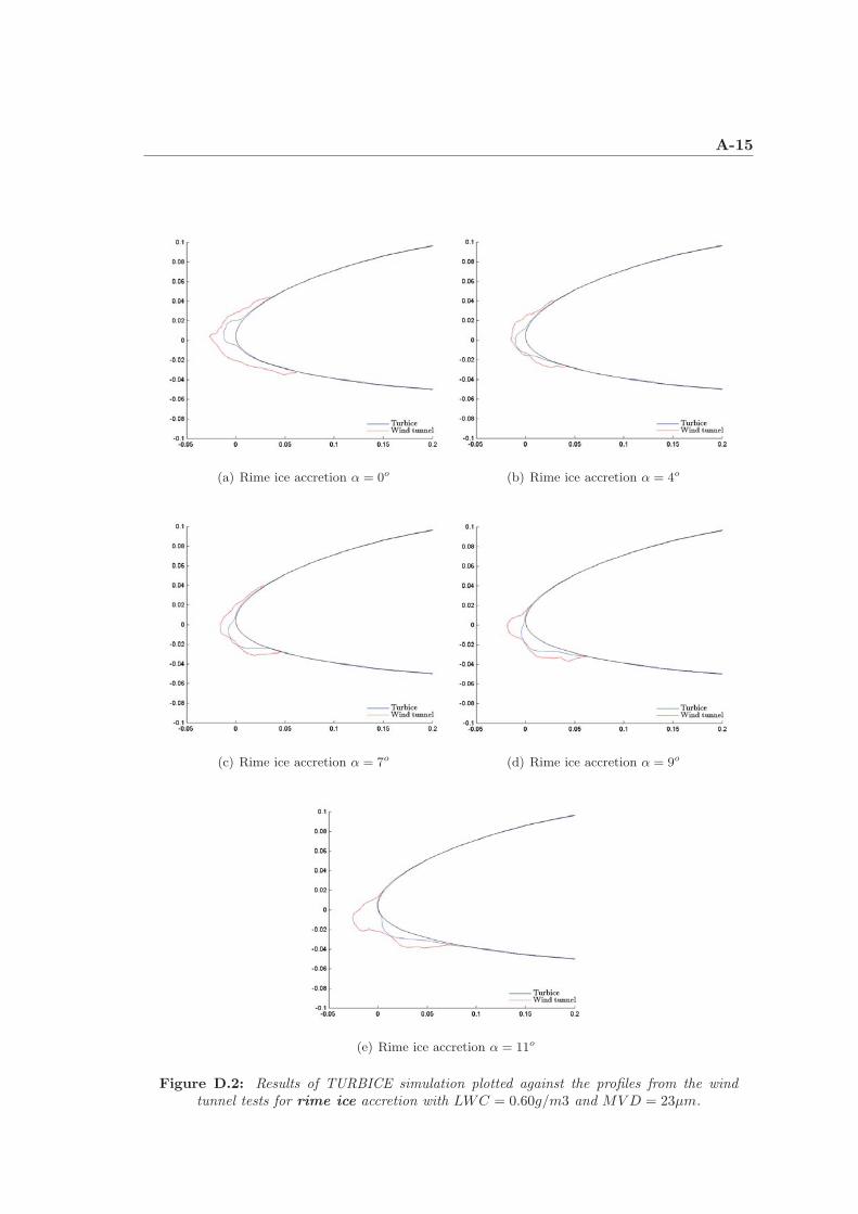
A-15
(a) Rime ice accretion α = 0o (b) Rime ice accretion α = 4o
(c) Rime ice accretion α = 7o (d) Rime ice accretion α = 9o
(e) Rime ice accretion α = 11o
Figure D.2: Results of TURBICE simulation plotted against the profiles from the windtunnel tests for rime ice accretion with LWC = 0.60g/m3 and MVD = 23μm.
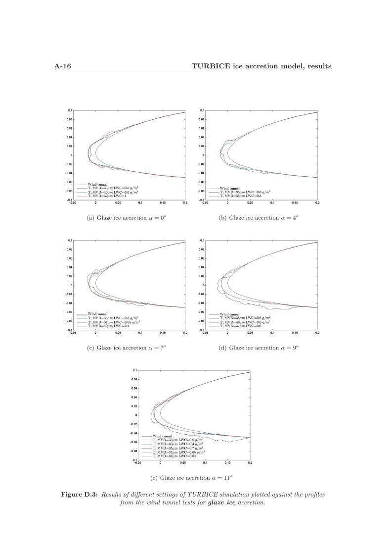
A-16 TURBICE ice accretion model, results
(a) Glaze ice accretion α = 0o (b) Glaze ice accretion α = 4o
(c) Glaze ice accretion α = 7o (d) Glaze ice accretion α = 9o
(e) Glaze ice accretion α = 11o
Figure D.3: Results of different settings of TURBICE simulation plotted against the profilesfrom the wind tunnel tests for glaze ice accretion.
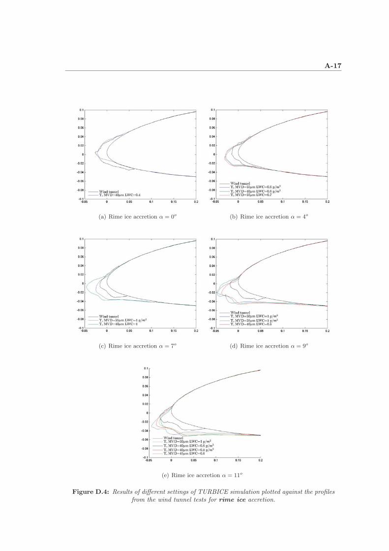
A-17
(a) Rime ice accretion α = 0o (b) Rime ice accretion α = 4o
(c) Rime ice accretion α = 7o (d) Rime ice accretion α = 9o
(e) Rime ice accretion α = 11o
Figure D.4: Results of different settings of TURBICE simulation plotted against the profilesfrom the wind tunnel tests for rime ice accretion.

A-18 TURBICE ice accretion model, results

Appendix E
Submitted and published papers
In this Appendix chapter, the submitted journal papers and published conference pro-ceeding are enclosed:
� Hudecz, A., Hansen, M. O. L., Dillingh, J. and Turkia, V., (2013). NumericalInvestigation of the Effects of Ice Accretion on a Wind Turbine Blade. Wind Energy.(Submitted)
� Hudecz, A., Koss, H. H. and Hansen, M. O. L., (2013). Icing Wind Tunnel Tests ofa Wind Turbine Blade. Wind Energy. (Submitted)
� Hudecz, A., Koss, H. H. and Hansen, M. O. L., (2013). Ice Accretion on Wind Tur-bine Blades. In XV. International Workshop on Atmospheric Icing on Structures,St-Johns, Newfoundland, September 8 to 11, 2013. (Oral presentation)
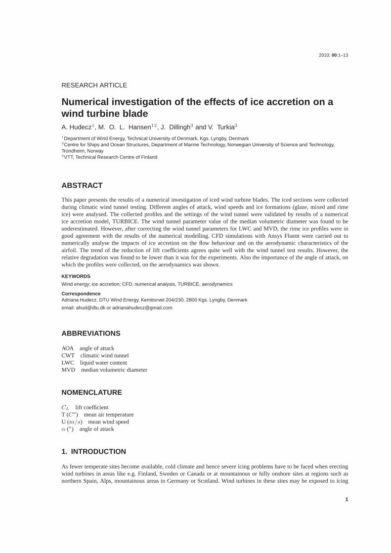
2010; 00:1–13
RESEARCH ARTICLE
Numerical investigation of the effects of ice accretion on awind turbine bladeA. Hudecz1, M. O. L. Hansen12, J. Dillingh3 and V. Turkia3
1Department of Wind Energy, Technical University of Denmark, Kgs. Lyngby, Denmark2Centre for Ships and Ocean Structures, Department of Marine Technology, Norwegian University of Science and Technology,Trondheim, Norway3VTT, Technical Research Centre of Finland
ABSTRACT
This paper presents the results of a numerical investigation of iced wind turbine blades. The iced sections were collectedduring climatic wind tunnel testing. Different angles of attack, wind speeds and ice formations (glaze, mixed and rimeice) were analysed. The collected profiles and the settings of the wind tunnel were validated by results of a numericalice accretion model, TURBICE. The wind tunnel parameter value of the median volumetric diameter was found to beunderestimated. However, after correcting the wind tunnel parameters for LWC and MVD, the rime ice profiles were ingood agreement with the results of the numerical modelling. CFD simulations with Ansys Fluent were carried out tonumerically analyse the impacts of ice accretion on the flow behaviour and on the aerodynamic characteristics of theairfoil. The trend of the reduction of lift coefficients agrees quite well with the wind tunnel test results. However, therelative degradation was found to be lower than it was for the experiments. Also the importance of the angle of attack, onwhich the profiles were collected, on the aerodynamics was shown.
KEYWORDSWind energy; ice accretion; CFD, numerical analysis, TURBICE, aerodynamics
CorrespondenceAdriana Hudecz, DTU Wind Energy, Kemitorvet 204/230, 2800 Kgs. Lyngby, Denmarkemail: [email protected] or [email protected]
ABBREVIATIONS
AOA angle of attackCWT climatic wind tunnelLWC liquid water contentMVD median volumetric diameter
NOMENCLATURE
CL lift coefficientT (Co) mean air temperatureU (m/s) mean wind speedα (o) angle of attack
1. INTRODUCTION
As fewer temperate sites become available, cold climate and hence severe icing problems have to be faced when erectingwind turbines in areas like e.g. Finland, Sweden or Canada or at mountainous or hilly onshore sites at regions such asnorthern Spain, Alps, mountainous areas in Germany or Scotland. Wind turbines in these sites may be exposed to icing
1
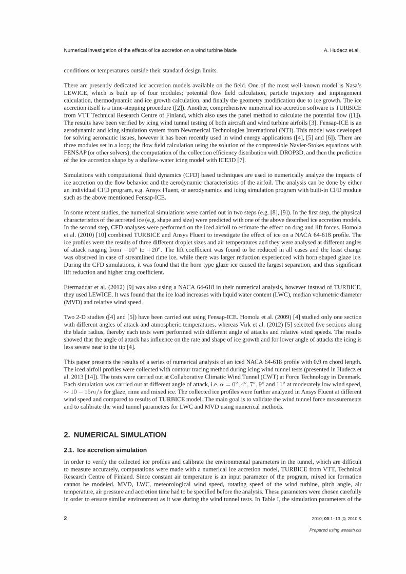
Numerical investigation of the effects of ice accretion on a wind turbine blade A. Hudecz et.al.
conditions or temperatures outside their standard design limits.
There are presently dedicated ice accretion models available on the field. One of the most well-known model is Nasa’sLEWICE, which is built up of four modules; potential flow field calculation, particle trajectory and impingementcalculation, thermodynamic and ice growth calculation, and finally the geometry modification due to ice growth. The iceaccretion itself is a time-stepping procedure ([2]). Another, comprehensive numerical ice accretion software is TURBICEfrom VTT Technical Research Centre of Finland, which also uses the panel method to calculate the potential flow ([1]).The results have been verified by icing wind tunnel testing of both aircraft and wind turbine airfoils [3]. Fensap-ICE is anaerodynamic and icing simulation system from Newmerical Technologies International (NTI). This model was developedfor solving aeronautic issues, however it has been recently used in wind energy applications ([4], [5] and [6]). There arethree modules set in a loop; the flow field calculation using the solution of the compressible Navier-Stokes equations withFENSAP (or other solvers), the computation of the collection efficiency distribution with DROP3D, and then the predictionof the ice accretion shape by a shallow-water icing model with ICE3D [7].
Simulations with computational fluid dynamics (CFD) based techniques are used to numerically analyze the impacts ofice accretion on the flow behavior and the aerodynamic characteristics of the airfoil. The analysis can be done by eitheran individual CFD program, e.g. Ansys Fluent, or aerodynamics and icing simulation program with built-in CFD modulesuch as the above mentioned Fensap-ICE.
In some recent studies, the numerical simulations were carried out in two steps (e.g. [8], [9]). In the first step, the physicalcharacteristics of the accreted ice (e.g. shape and size) were predicted with one of the above described ice accretion models.In the second step, CFD analyses were performed on the iced airfoil to estimate the effect on drag and lift forces. Homolaet al. (2010) [10] combined TURBICE and Ansys Fluent to investigate the effect of ice on a NACA 64-618 profile. Theice profiles were the results of three different droplet sizes and air temperatures and they were analysed at different anglesof attack ranging from −10o to +20o. The lift coefficient was found to be reduced in all cases and the least changewas observed in case of streamlined rime ice, while there was larger reduction experienced with horn shaped glaze ice.During the CFD simulations, it was found that the horn type glaze ice caused the largest separation, and thus significantlift reduction and higher drag coefficient.
Etermaddar et al. (2012) [9] was also using a NACA 64-618 in their numerical analysis, however instead of TURBICE,they used LEWICE. It was found that the ice load increases with liquid water content (LWC), median volumetric diameter(MVD) and relative wind speed.
Two 2-D studies ([4] and [5]) have been carried out using Fensap-ICE. Homola et al. (2009) [4] studied only one sectionwith different angles of attack and atmospheric temperatures, whereas Virk et al. (2012) [5] selected five sections alongthe blade radius, thereby each tests were performed with different angle of attacks and relative wind speeds. The resultsshowed that the angle of attack has influence on the rate and shape of ice growth and for lower angle of attacks the icing isless severe near to the tip [4].
This paper presents the results of a series of numerical analysis of an iced NACA 64-618 profile with 0.9 m chord length.The iced airfoil profiles were collected with contour tracing method during icing wind tunnel tests (presented in Hudecz etal. 2013 [14]). The tests were carried out at Collaborative Climatic Wind Tunnel (CWT) at Force Technology in Denmark.Each simulation was carried out at different angle of attack, i.e. α = 0o, 4o, 7o, 9o and 11o at moderately low wind speed,∼ 10− 15m/s for glaze, rime and mixed ice. The collected ice profiles were further analyzed in Ansys Fluent at differentwind speed and compared to results of TURBICE model. The main goal is to validate the wind tunnel force measurementsand to calibrate the wind tunnel parameters for LWC and MVD using numerical methods.
2. NUMERICAL SIMULATION
2.1. Ice accretion simulation
In order to verify the collected ice profiles and calibrate the environmental parameters in the tunnel, which are difficultto measure accurately, computations were made with a numerical ice accretion model, TURBICE from VTT, TechnicalResearch Centre of Finland. Since constant air temperature is an input parameter of the program, mixed ice formationcannot be modeled. MVD, LWC, meteorological wind speed, rotating speed of the wind turbine, pitch angle, airtemperature, air pressure and accretion time had to be specified before the analysis. These parameters were chosen carefullyin order to ensure similar environment as it was during the wind tunnel tests. In Table I, the simulation parameters of the
2 2010; 00:1–13 c© 2010 &
Prepared using weauth.cls

A. Hudecz et.al. Numerical investigation of the effects of ice accretion on a wind turbine blade
validation tests in TURBICE are listed. MVD and LWC are target values, which were set in the tunnel and the listedtemperatures and wind speeds are mean temperature and velocity, which were achieved during the ice accretion.
Table I. Input parameters of validation tests done with TURBICE
Parameters Glaze ice Rime iceI. II. III. IV. V. I. II. III. IV. V.
AOA (o) 0 4 7 9 11 0 4 7 9 11MVD (μm) 27 27 27 27 27 23 23 23 23 23
LWC (g/m3) 0.65 0.65 0.65 0.65 0.65 0.6 0.6 0.6 0.6 0.6T (oC) -3 -3 -3 -3 -3 -8 -8 -8 -8 -8U (m/s) 15 15 15 15 15 10 10 10 10 10
Time (min) 60 60 60 60 60 60 60 60 60 60
2.2. Computational fluid dynamics
Simulations with Ansys Fluent were afterwards conducted to quantify the impacts of ice accretion on the flow behaviorand the aerodynamic characteristics of the iced airfoil from the wind tunnel tests. First, the aerodynamic forces measuredduring the experiments were verified. Due to the limitation of the CWT’s cooling unit, it was necessary to set relativelylow target wind speed (15 m/s which corresponds to appr. Re = 1E6) to ensure stable and low enough air temperature.A number of numerical tests were done with higher wind speed, 25 m/s (Re = 1.5E6). For each simulation, each of theice deposit accreted at the same AOA as the investigation of the flow behaviour and the aerodynamic characteristics wasdone. These tests are refereed as ”dedicated profile” tests or simulations.
The impact of angle of attack was investigated with one single profile. For this investigation, the glaze and rime iced airfoilscollected at α = 0o and 11o were chosen and they were tested in flows with 0o, 4o, 7o, 9o and 11o incident angles and 25m/s wind speed. These tests are refereed as ”single profile” tests or simulations.
The ice profiles were collected from specific spanwise locations, and therefore a 2-D model was done in Ansys Workbench.The control volume around the airfoil was rectangular with edges positioned at 50 chords length away in vertical directionand 20 chords length from the horizontal direction.
An inflation layer was added to the mesh to produce a structured, fine mesh in the vicinity of the airfoil to achieve thedesired wall Y + distribution and thus give a better representation of the flow near the airfoil surface, see examples forα = 0o in Figure 1. The first layer height is dependent on the surface roughness, since the roughness height may notexceed it. However, it was found that Ansys Fluent cannot properly handle micro surface roughness, therefore it was notincluded in the analysis and only the large scale roughness resolved in the grid is felt by the flow. It was aimed to constructsimilar mesh and also inflation layer for all the different profiles, but sometimes due to the complexity of the curve of theice shapes, minor changes had to be done. In Table II, the set-up of mesh and inflation layer of each test is summarized.
For the simulations, fully turbulent flow was assumed considering the roughness of the ice deposit. Spalart-Allmaras andk − ω SST turbulence models were used. It was found in previous studies [11] that the solution converges faster and easierusing Spalart-Allmaras model than with the k − ω SST turbulence model. Therefore for the clean profiles, the first 500iterations were done by using Spalart-Allmaras model providing an initial guess for the k − ω SST turbulence model andachieving more stable convergence. However, it was shown by Chung and Addy (2000) [12] that Spalart-Allmaras modelis the best performing model when simulating ice accretions and hence it was used during the iced profiles’ analysis. In all5000 iteration were done to ensure stable solution.
3. RESULTS
3.1. Ice accretion simulation
The aim of the TURBICE tests was to validate the collected ice profiles and the setting of the meteorological variables,especially MVD and LWC. Therefore a set of simulations were performed using the same input parameters as the target
2010; 00:1–13 c© 2010 & 3
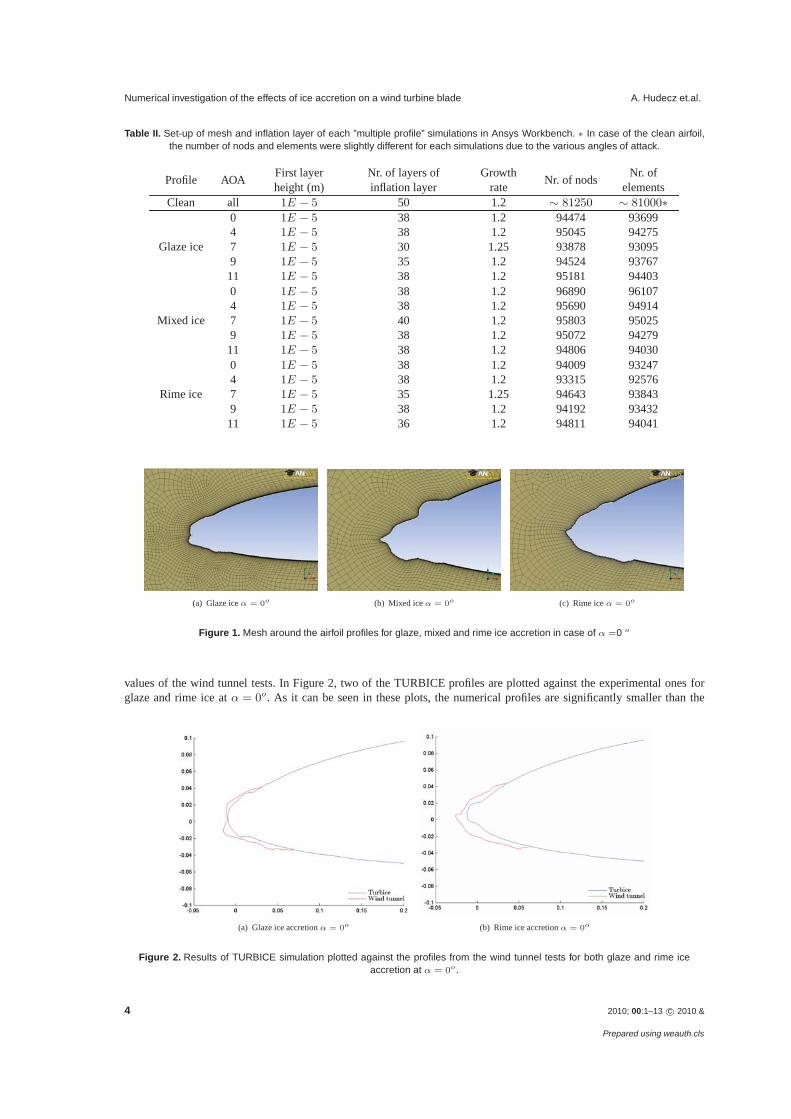
Numerical investigation of the effects of ice accretion on a wind turbine blade A. Hudecz et.al.
Table II. Set-up of mesh and inflation layer of each ”multiple profile” simulations in Ansys Workbench. ∗ In case of the clean airfoil,the number of nods and elements were slightly different for each simulations due to the various angles of attack.
Profile AOA First layerheight (m)
Nr. of layers ofinflation layer
Growthrate Nr. of nods Nr. of
elementsClean all 1E − 5 50 1.2 ∼ 81250 ∼ 81000∗
Glaze ice
0 1E − 5 38 1.2 94474 936994 1E − 5 38 1.2 95045 942757 1E − 5 30 1.25 93878 930959 1E − 5 35 1.2 94524 9376711 1E − 5 38 1.2 95181 94403
Mixed ice
0 1E − 5 38 1.2 96890 961074 1E − 5 38 1.2 95690 949147 1E − 5 40 1.2 95803 950259 1E − 5 38 1.2 95072 9427911 1E − 5 38 1.2 94806 94030
Rime ice
0 1E − 5 38 1.2 94009 932474 1E − 5 38 1.2 93315 925767 1E − 5 35 1.25 94643 938439 1E − 5 38 1.2 94192 9343211 1E − 5 36 1.2 94811 94041
(a) Glaze ice α = 0o (b) Mixed ice α = 0o (c) Rime ice α = 0o
Figure 1. Mesh around the airfoil profiles for glaze, mixed and rime ice accretion in case of α =0 o
values of the wind tunnel tests. In Figure 2, two of the TURBICE profiles are plotted against the experimental ones forglaze and rime ice at α = 0o. As it can be seen in these plots, the numerical profiles are significantly smaller than the
(a) Glaze ice accretion α = 0o (b) Rime ice accretion α = 0o
Figure 2. Results of TURBICE simulation plotted against the profiles from the wind tunnel tests for both glaze and rime iceaccretion at α = 0o.
4 2010; 00:1–13 c© 2010 &
Prepared using weauth.cls
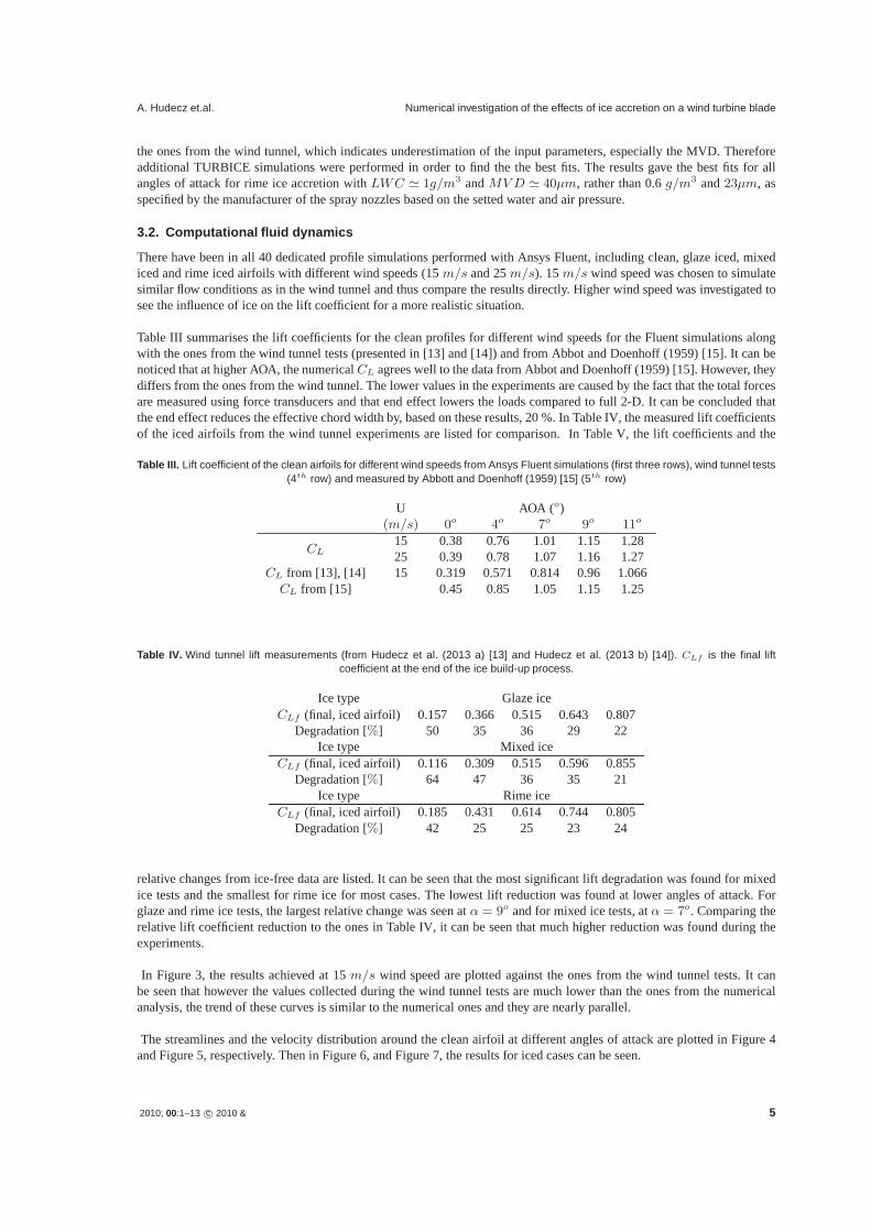
A. Hudecz et.al. Numerical investigation of the effects of ice accretion on a wind turbine blade
the ones from the wind tunnel, which indicates underestimation of the input parameters, especially the MVD. Thereforeadditional TURBICE simulations were performed in order to find the the best fits. The results gave the best fits for allangles of attack for rime ice accretion with LWC � 1g/m3 and MVD � 40μm, rather than 0.6 g/m3 and 23μm, asspecified by the manufacturer of the spray nozzles based on the setted water and air pressure.
3.2. Computational fluid dynamics
There have been in all 40 dedicated profile simulations performed with Ansys Fluent, including clean, glaze iced, mixediced and rime iced airfoils with different wind speeds (15 m/s and 25 m/s). 15 m/s wind speed was chosen to simulatesimilar flow conditions as in the wind tunnel and thus compare the results directly. Higher wind speed was investigated tosee the influence of ice on the lift coefficient for a more realistic situation.
Table III summarises the lift coefficients for the clean profiles for different wind speeds for the Fluent simulations alongwith the ones from the wind tunnel tests (presented in [13] and [14]) and from Abbot and Doenhoff (1959) [15]. It can benoticed that at higher AOA, the numerical CL agrees well to the data from Abbot and Doenhoff (1959) [15]. However, theydiffers from the ones from the wind tunnel. The lower values in the experiments are caused by the fact that the total forcesare measured using force transducers and that end effect lowers the loads compared to full 2-D. It can be concluded thatthe end effect reduces the effective chord width by, based on these results, 20 %. In Table IV, the measured lift coefficientsof the iced airfoils from the wind tunnel experiments are listed for comparison. In Table V, the lift coefficients and the
Table III. Lift coefficient of the clean airfoils for different wind speeds from Ansys Fluent simulations (first three rows), wind tunnel tests(4th row) and measured by Abbott and Doenhoff (1959) [15] (5th row)
U AOA (o)(m/s) 0o 4o 7o 9o 11o
CL15 0.38 0.76 1.01 1.15 1.2825 0.39 0.78 1.07 1.16 1.27
CL from [13], [14] 15 0.319 0.571 0.814 0.96 1.066CL from [15] 0.45 0.85 1.05 1.15 1.25
Table IV. Wind tunnel lift measurements (from Hudecz et al. (2013 a) [13] and Hudecz et al. (2013 b) [14]). CLf is the final liftcoefficient at the end of the ice build-up process.
Ice type Glaze iceCLf (final, iced airfoil) 0.157 0.366 0.515 0.643 0.807
Degradation [%] 50 35 36 29 22Ice type Mixed ice
CLf (final, iced airfoil) 0.116 0.309 0.515 0.596 0.855Degradation [%] 64 47 36 35 21
Ice type Rime iceCLf (final, iced airfoil) 0.185 0.431 0.614 0.744 0.805
Degradation [%] 42 25 25 23 24
relative changes from ice-free data are listed. It can be seen that the most significant lift degradation was found for mixedice tests and the smallest for rime ice for most cases. The lowest lift reduction was found at lower angles of attack. Forglaze and rime ice tests, the largest relative change was seen at α = 9o and for mixed ice tests, at α = 7o. Comparing therelative lift coefficient reduction to the ones in Table IV, it can be seen that much higher reduction was found during theexperiments.
In Figure 3, the results achieved at 15 m/s wind speed are plotted against the ones from the wind tunnel tests. It canbe seen that however the values collected during the wind tunnel tests are much lower than the ones from the numericalanalysis, the trend of these curves is similar to the numerical ones and they are nearly parallel.
The streamlines and the velocity distribution around the clean airfoil at different angles of attack are plotted in Figure 4and Figure 5, respectively. Then in Figure 6, and Figure 7, the results for iced cases can be seen.
2010; 00:1–13 c© 2010 & 5
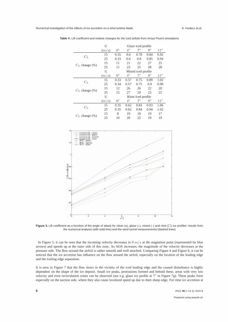
Numerical investigation of the effects of ice accretion on a wind turbine blade A. Hudecz et.al.
Table V. Lift coefficient and relative changes for the iced airfoils from Ansys Fluent simulations
U Glaze iced profile(m/s) 0o 4o 7o 9o 11o
CL15 0.35 0.6 0.78 0.84 0.9225 0.33 0.6 0.8 0.85 0.94
CL change (%) 15 11 21 22 27 2525 11 23 25 28 28U Mixed iced profile
(m/s) 0o 4o 7o 9o 11o
CL15 0.33 0.57 0.75 0.89 1.0225 0.34 0.57 0.75 0.9 0.99
CL change (%) 15 12 26 26 22 2025 15 27 29 23 22U Rime iced profile
(m/s) 0o 4o 7o 9o 11o
CL15 0.35 0.62 0.83 0.93 1.0625 0.35 0.62 0.84 0.94 1.02
CL change (%) 15 8 19 18 19 1725 10 20 22 19 19
Figure 3. Lift coefficient as a function of the angle of attack for clean (•), glaze (∗), mixed (◦) and rime (�) ice profiles’ results fromthe numerical analysis (with solid line) and the wind tunnel measurements (dashed lines)
In Figure 5, it can be seen that the incoming velocity decreases to 0 m/s at the stagnation point (represented by bluearrows) and speeds up at the outer side of this zone. As AOA increases, the magnitude of the velocity decreases at thepressure side. The flow around the airfoil is rather smooth and well attached. Comparing Figure 4 and Figure 6, it can benoticed that the ice accretion has influence on the flow around the airfoil, especially on the location of the leading edgeand the trailing edge separation.
It is seen in Figure 7 that the flow slows in the vicinity of the iced leading edge and the caused disturbance is highlydependent on the shape of the ice deposit. Small ice peaks, protrusions formed and behind these, areas with very lowvelocity and even recirculation zones can be observed (see e.g. glaze ice profile at 7o in Figure 7g). These peaks formespecially on the suction side, where they also cause localized speed up due to their sharp edge. For rime ice accretion at
6 2010; 00:1–13 c© 2010 &
Prepared using weauth.cls
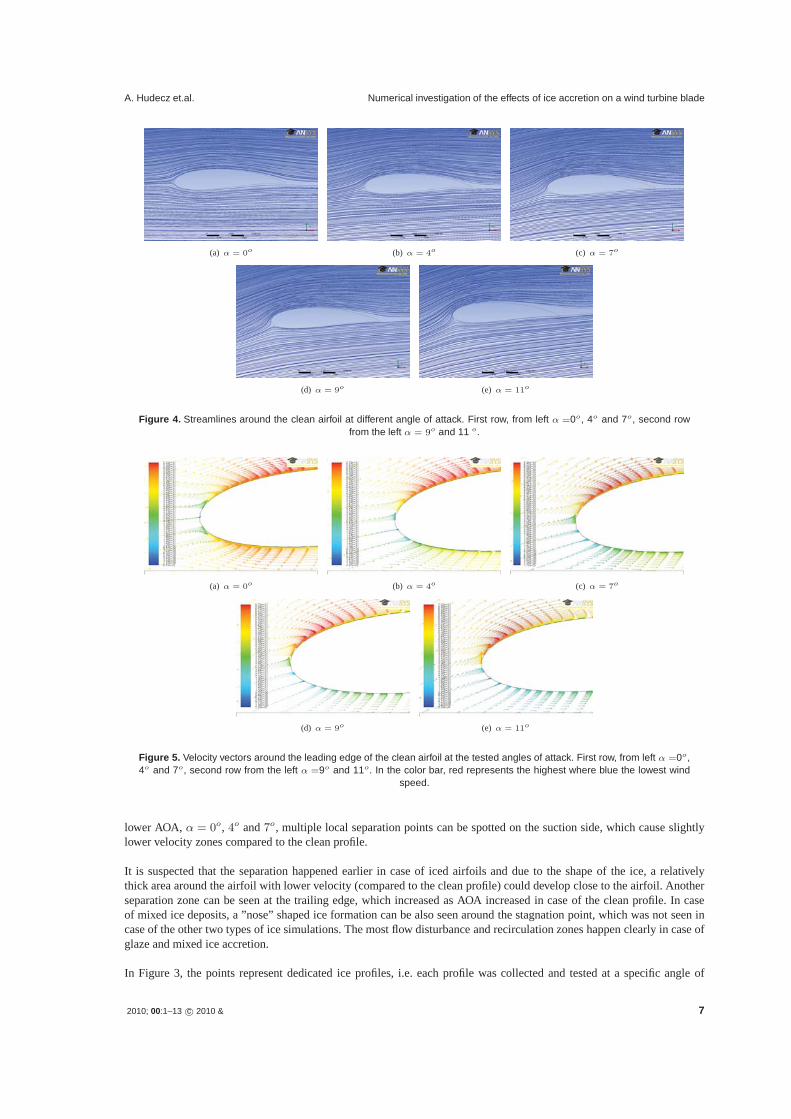
A. Hudecz et.al. Numerical investigation of the effects of ice accretion on a wind turbine blade
(a) α = 0o (b) α = 4o (c) α = 7o
(d) α = 9o (e) α = 11o
Figure 4. Streamlines around the clean airfoil at different angle of attack. First row, from left α =0o, 4o and 7o, second rowfrom the left α = 9o and 11 o.
(a) α = 0o (b) α = 4o (c) α = 7o
(d) α = 9o (e) α = 11o
Figure 5. Velocity vectors around the leading edge of the clean airfoil at the tested angles of attack. First row, from left α =0o,4o and 7o, second row from the left α =9o and 11o. In the color bar, red represents the highest where blue the lowest wind
speed.
lower AOA, α = 0o, 4o and 7o, multiple local separation points can be spotted on the suction side, which cause slightlylower velocity zones compared to the clean profile.
It is suspected that the separation happened earlier in case of iced airfoils and due to the shape of the ice, a relativelythick area around the airfoil with lower velocity (compared to the clean profile) could develop close to the airfoil. Anotherseparation zone can be seen at the trailing edge, which increased as AOA increased in case of the clean profile. In caseof mixed ice deposits, a ”nose” shaped ice formation can be also seen around the stagnation point, which was not seen incase of the other two types of ice simulations. The most flow disturbance and recirculation zones happen clearly in case ofglaze and mixed ice accretion.
In Figure 3, the points represent dedicated ice profiles, i.e. each profile was collected and tested at a specific angle of
2010; 00:1–13 c© 2010 & 7
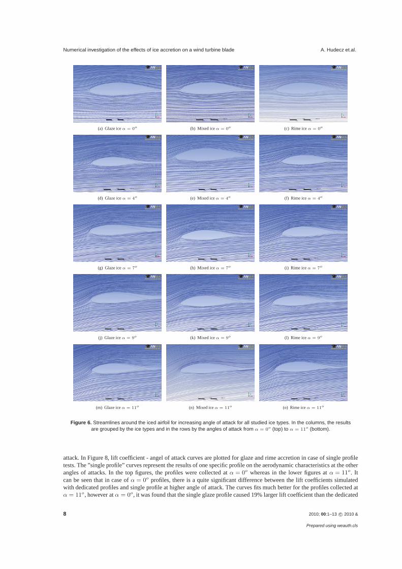
Numerical investigation of the effects of ice accretion on a wind turbine blade A. Hudecz et.al.
(a) Glaze ice α = 0o (b) Mixed ice α = 0o (c) Rime ice α = 0o
(d) Glaze ice α = 4o (e) Mixed ice α = 4o (f) Rime ice α = 4o
(g) Glaze ice α = 7o (h) Mixed ice α = 7o (i) Rime ice α = 7o
(j) Glaze ice α = 9o (k) Mixed ice α = 9o (l) Rime ice α = 9o
(m) Glaze ice α = 11o (n) Mixed ice α = 11o (o) Rime ice α = 11o
Figure 6. Streamlines around the iced airfoil for increasing angle of attack for all studied ice types. In the columns, the resultsare grouped by the ice types and in the rows by the angles of attack from α = 0o (top) to α = 11o (bottom).
attack. In Figure 8, lift coefficient - angel of attack curves are plotted for glaze and rime accretion in case of single profiletests. The ”single profile” curves represent the results of one specific profile on the aerodynamic characteristics at the otherangles of attacks. In the top figures, the profiles were collected at α = 0o whereas in the lower figures at α = 11o. Itcan be seen that in case of α = 0o profiles, there is a quite significant difference between the lift coefficients simulatedwith dedicated profiles and single profile at higher angle of attack. The curves fits much better for the profiles collected atα = 11o, however at α = 0o, it was found that the single glaze profile caused 19% larger lift coefficient than the dedicated
8 2010; 00:1–13 c© 2010 &
Prepared using weauth.cls
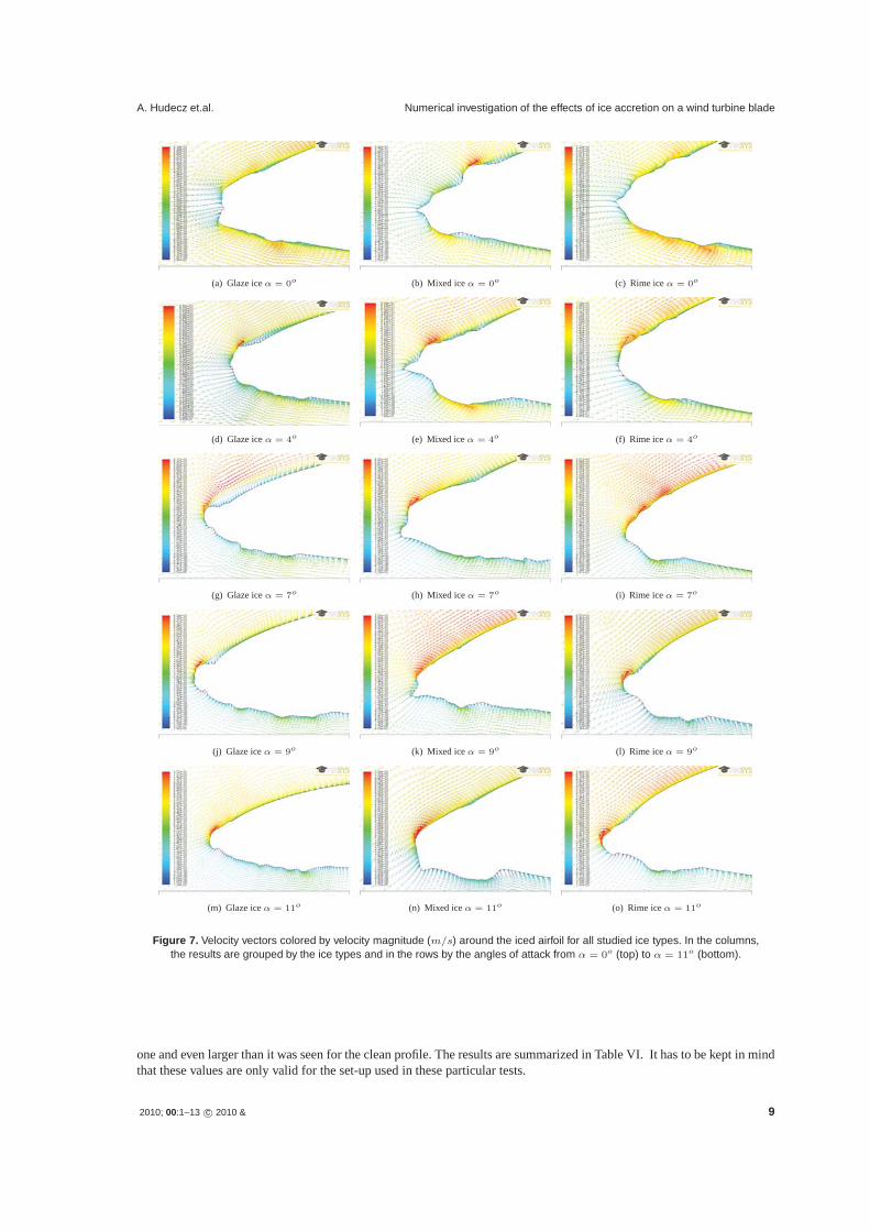
A. Hudecz et.al. Numerical investigation of the effects of ice accretion on a wind turbine blade
(a) Glaze ice α = 0o (b) Mixed ice α = 0o (c) Rime ice α = 0o
(d) Glaze ice α = 4o (e) Mixed ice α = 4o (f) Rime ice α = 4o
(g) Glaze ice α = 7o (h) Mixed ice α = 7o (i) Rime ice α = 7o
(j) Glaze ice α = 9o (k) Mixed ice α = 9o (l) Rime ice α = 9o
(m) Glaze ice α = 11o (n) Mixed ice α = 11o (o) Rime ice α = 11o
Figure 7. Velocity vectors colored by velocity magnitude (m/s) around the iced airfoil for all studied ice types. In the columns,the results are grouped by the ice types and in the rows by the angles of attack from α = 0o (top) to α = 11o (bottom).
one and even larger than it was seen for the clean profile. The results are summarized in Table VI. It has to be kept in mindthat these values are only valid for the set-up used in these particular tests.
2010; 00:1–13 c© 2010 & 9
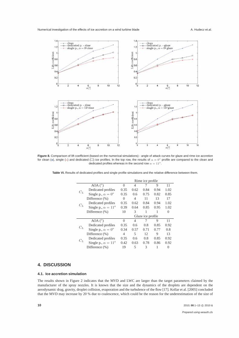
Numerical investigation of the effects of ice accretion on a wind turbine blade A. Hudecz et.al.
Figure 8. Comparison of lift coefficient (based on the numerical simulations) - angle of attack curves for glaze and rime ice accretionfor clean (•), single (∗) and dedicated (�) ice profiles. In the top row, the results of α = 0o profile are compared to the clean and
dedicated profiles whereas in the second row α = 11o.
Table VI. Results of dedicated profiles and single profile simulations and the relative difference between them.
Rime ice profileAOA (o) 0 4 7 9 11
CLDedicated profiles 0.35 0.62 0.84 0.94 1.02Single p., α = 0o 0.35 0.6 0.75 0.82 0.85
Difference (%) 0 4 11 13 17
CLDedicated profiles 0.35 0.62 0.84 0.94 1.02Single p., α = 11o 0.39 0.64 0.85 0.95 1.02
Difference (%) 10 3 1 1 0Glaze ice profile
AOA (o) 0 4 7 9 11
CLDedicated profiles 0.35 0.6 0.8 0.85 0.92Single p., α = 0o 0.34 0.57 0.71 0.77 0.8
Difference (%) 4 5 12 9 13
CLDedicated profiles 0.35 0.6 0.8 0.85 0.92Single p., α = 11o 0.42 0.63 0.78 0.86 0.92
Difference (%) 19 5 3 1 0
4. DISCUSSION
4.1. Ice accretion simulation
The results shown in Figure 2 indicates that the MVD and LWC are larger than the target parameters claimed by themanufacturer of the spray nozzles. It is known that the size and the dynamics of the droplets are dependent on theaerodynamic drag, gravity, droplet collision, evaporation and the turbulence of the flow [17]. Kollar et al. [2005] concludedthat the MVD may increase by 20 % due to coalescence, which could be the reason for the underestimation of the size of
10 2010; 00:1–13 c© 2010 &
Prepared using weauth.cls
A. Hudecz et.al. Numerical investigation of the effects of ice accretion on a wind turbine blade
the droplets which impinged on the surface of the airfoil. At low air speeds such as 5-10 m/s, the gravity has significantinfluence on the vertical deflection of the droplet trajectories, causing gravitational sedimentation. The vertical deflectionof the droplet trajectories has influence on the vertical LWC distribution, i.e. the maximum LWC occurs at lower height.It could cause the thick ice deposit in case of the experimental glaze ice accretion at higher angles of attack since as theAOA is increased the larger the surface area, which faces the flow.
Additional simulations suggest that in case of rime ice profiles, the numerical profiles agree well with the experimentalones, if LWC is increased to 1g/m3 and the MVD to 40μm.
4.2. Computational fluid dynamics
The results of the dedicated and single profile tests are discussed separately in this section.
4.2.1. Simulations with dedicated profilesThe lift coefficient - angle of attack curves from the numerical analyses are qualitatively in good agreement with the
ones from the wind tunnel tests, as shown in Figure 3. However, the values from the wind tunnel are much lower than theones from the numerical simulations due to the fact that these data were only corrected for lift interference and blockageinterference but not for the presence of end effect from the vertical walls. In case of the iced airfoils, another reason forthese differences could be that with the contour tracing method, the small changes of surface roughness could not bedocumented therefore they were not implemented in the numerical analysis, and it was shown in many studies (e.g. [16])that it has significant effect on the aerodynamics of the airfoil. Based on the differences in the aerodynamic effect between2-D and 3-D ice shapes, Addy (2000) [18] concluded that the surface roughness and the irregularities present in naturalaircraft ice are important characteristics. These could also cause the differences between the results of the wind tunnel testsand the numerical simulations.
A comparison was made between the clean airfoil lift coefficients of the wind tunnel tests and the numerical simulationsalong with the CL values presented by Abbott and Doenhoff (1959) [15], which implies that it is likely that the end effectcaused by the vertical walls led to an approximately 20 % reduction in the effective width of the airfoil section.
The measured relative reduction of lift coefficient (listed in Table IV) shows also quite large difference from the ones listedin Table V, which implies that the combination of the presence of the wind tunnel’s vertical walls and the changed surfaceroughness had significant influence on the measurements. For lower angles of attack, especially α = 0o, the differencebetween the measured and simulated relative reduction is significantly large, which indicates that the altered surfaceroughness had the highest influence on the lift reduction.
Similarly to e.g. Homola et al. (2010) [10], lift was found to decrease in all cases. E.g. Virk et al. (2010) [19] found ahigher value of lift coefficient for rime iced profiles than for the clean profiles due to the increased effective chord lengthand camber of the blade profile. This was not experienced in the presented cases of dedicated profile simulations. However,as it can be seen in Figure 7, the curvature of the ice shapes follows well with the curve of the airfoil at the suction side,i.e. acts as an extended leading edge, and thus could cause less significant lift degradation than e.g. the glaze ice accretion.
A tendency of increased lift reduction was seen for glaze ice accretion as the AOA increased. This is due to thecharacteristics of glaze ice. During glaze ice accretion, because of the relatively higher air temperature (0−−4oC),not all water droplets freeze to the surface on impact and hence some run along the airfoil and freeze later [20]. As AOAincreases, the area exposed to the water droplets increases as well, therefore it causes more flow disturbance and thus morelift reduction.
In most of the cases, mixed ice accretion caused more significant lift degradation than glaze ice accretion due to the largeice deposit, which accumulated on the leading edge and hence higher flow disturbance (see Figure 7).
A significant change in the flow pattern was observed, when a comparison was made between clean and iced blade profilesdue to the changes of the aerodynamically shaped leading edge curve. As ice built up on the leading edge, the surface area,which faced the incoming flow and thus the water droplets, increased, causing major flow disturbance.
4.2.2. Simulations with single profilesThe impact of single ice profiles collected at α = 0o and α = 11o were studied at different angles of attack. The lift
coefficients of α = 0o for both glaze and rime ice accretion are lower than the ones found in case of dedicated profile tests.The reason for this difference could be that ice was accumulated only on the leading edge in case of α = 0o and when
2010; 00:1–13 c© 2010 & 11
Numerical investigation of the effects of ice accretion on a wind turbine blade A. Hudecz et.al.
the incident angle of incoming flow is increased, the stagnation point moves downstream of the ice deposit disturbing theflow on the suction side, which has higher influence on the lift coefficient than the pressure side. The profiles collectedat α = 11o did not cause significantly different lift curves from the multiple profiles because for α < 11o values, the icedeposit is downstream of the stagnation point. However at α = 0o, the lift coefficient got larger for the single profile.
5. CONCLUSION
A two phases numerical analysis has been performed to study the effect of glaze, rime and mixed ice accretion on theaerodynamics of an iced NACA 64-618 airfoil. The profiles were collected from icing wind tunnel tests. In the firstphase, validation of the collected profiles and the environmental conditions were done by numerical ice accretion model,TURBICE from VTT, Research Centre of Finland. CFD simulations with Ansys Fluent were carried out to numericallyanalyse the impacts of ice accretion on the flow behaviour and on the aerodynamic characteristics of the airfoil withdifferent wind velocities.
The TURBICE simulations showed that the values of the median volumetric diameter and liquid water content in thewind tunnel were underestimated. The resulted MVD was significantly larger than the target value due to the applied lowwind speed and thus coalescence of the water droplets. Vertical deflection of the droplet trajectories had influence on thevertical LWC distribution, which lead to more ice accumulation on the pressure side than it was found during the numericalsimulation.
Comparison between the measured and the numerical lift coefficient of the clean airfoil suggests that presence of thevertical walls reduced the effective width of airfoil by approximately 20 %. The results of the CFD analyses of the icedairfoils imply that the combination of the presence of the vertical wall of the wind tunnel and the changed surface roughnesshad significant influence on the measurements. However, the trend of the lift coefficient - angle of attack curves from thenumerical analyses are in good agreement with the ones from the wind tunnel tests. A significant change in the flowpattern was observed, when a comparison was made between clean and iced blade profiles due to the changes of theaerodynamically shaped leading edge curve.
The importance of the angle of attack, on which the profiles were collected, on the lift coefficient was shown. The resultsof the single profile tests in case of α = 0o for both glaze and rime ice accretion gave lower lift coefficients than the onesfor dedicated profile tests.
In future work, a proper implementation of the surface roughness and also the runback ice rivulets is suggested in order toeliminate the errors caused by the lack of surface roughness.
ACKNOWLEDGMENT
VTT, Technical Research Centre of Finland is acknowledged for the support they provided for using TURBICE iceaccretion model and also performing additional simulations.
REFERENCES
1. Makkonen L., Laakso T., Marjaniemi M., and Finstad K. J. Modeling and prevention of ice accretion on wind turbines.Wind Energy, 25(1):3-21, 2001.
2. Wright W. B., Potapczuk M. G., and Levinson L. H. Comparison of LEWICE and Glenn ICE in the SLD Regime. In46th Aerospace Sciences Meeting and Exhibit, Reno, Nevada, January 7-10, 2008.
3. Homola M. C., Wallenius T., Makkonen L., Nicklasson P. J., and Sundsb P. A. Turbine Size and TemperatureDependence of Icing on Wind Turbine Blades. Wind Engineering, 34(6):615-628, 2010.
4. Homola M. C., Wallenius T., Makkonen L., and Nicklasson P. J. The relationship between chord length and rime icingon wind turbines. Wind Energy, 13(7):627-632, 2009.
5. Virk M. S., Homola M. C., and Nicklasson P. J. Atmospheric icing on large wind turbine blades. International Journalof Energy and Environment, 3(1):1-8, 2012.
6. Reid T., Baruzz G., Switchenko D. and Habashi W. G. FENSAP-ICE Simulation of Icing on Wind Turbine Blades,Part 1: Performance Degradation. 51st AIAA Aerospace Sciences Meeting including the New Horizons Forum andAerospace Exposition 07 - 10 January 2013, Grapevine (Dallas/Ft. Worth Region), Texas
12 2010; 00:1–13 c© 2010 &
Prepared using weauth.cls

A. Hudecz et.al. Numerical investigation of the effects of ice accretion on a wind turbine blade
7. Habashi W. G., Morency F., and Beaugendre H. FENSAP-ICE: a comprehensive 3D Simulation Tool for Inflight Icing.In 7th International Congress of Fluid Dynamics and Propulsion, Sharm-El-Sheikh, Egypt, December, 2001.
8. Virk M. S., Homola M. C., and Nicklasson P. J. Effect of Rime Ice Accretion on Aerodynamic Characteristics of WindTurbine Blade Profiles. Wind Engineering, 34(2):207-218, Mar. 2010.
9. Etemaddar M., Hansen M. O. L., and Moan T. Wind turbine aerodynamic response under atmospheric icing conditions.Wind Energy, 2012.
10. Homola M. C., Virk M. S., Wallenius T., Nicklasson P. J., and Sundsb P. A. Effect of atmospheric temperatureand droplet size variation on ice accretion of wind turbine blades. Journal of Wind Engineering and IndustrialAerodynamics, 98(12):724-729, 2010b.
11. Mortensen K. CFD Simulation of an airfoil with leading edge ice accretion. Master thesis. Department of MechanicalEngineering, Technical University of Denmark, 2008.
12. Chung J. J.and Addy, H. E. A Numerical Evaluation of Icing effects on a Natural Laminar Flow Airfoil. NASA TM-2000-209775, January 2000.
13. Hudecz A., Koss, H. and Hansen, M. O. L. Ice Accretion on Wind Turbine Blades. IWAIS XV, St-Johns, Newfoundland,September 8-11, 2013
14. Hudecz A., Koss, H. and Hansen, M. O. L.Icing Wind Tunnel Tests of a Wind Turbine Blade. Submitted paper15. Abbott I. and von Doenhoff A. Theory of Wing Sections. Including a Summary of AirfoilData. Courier Dover
Publications, 1959.16. Bragg M, Broeren A. P, and Blumenthal L. Iced-airfoil aerodynamics. Progress in Aerospace Sciences 2005,
41(5):323-362.17. Kollar L. E., Farzaneh M., and Karev A. R. Modeling droplet collision and coalescence in an icing wind tunnel and
the influence of these processes on droplet size distribution. International Journal of Multiphase Flow, 31(1):69-92,2005.
18. Addy, H. E. Jr, Ice Accretions and Icing Effects for Modern Airfoils. Technical report. NASA TM-2000-209775, April2000.
19. Virk M. S., Homola M. C., and Nicklasson P. J. Relation Between Angle of Attack and Atmospheric Ice Accretion onLarge Wind Turbine’s Blade. Wind Engineering, 34(6):607-614, 2010.
20. Bose N. Icing on a small horizontal-axis wind turbine - Part 1: Glaze ice profiles. Journal of Wind Engineering andIndustrial Aerodynamics 1992, 45:7585.
2010; 00:1–13 c© 2010 & 13

2010; 00:1–14
RESEARCH ARTICLE
Icing wind tunnel tests of a wind turbine bladeA. Hudecz1, H. Koss2 and M. O. L. Hansen13
1Department of Wind Energy, Technical University of Denmark, Kgs. Lyngby, Denmark2Department of Civil Engineering, Technical University of Denmark, Kgs. Lyngby, Denmark3Centre for Ships and Ocean Structures, Department of Marine
ABSTRACT
Wind tunnel tests were performed to investigate how ice accumulates for moderate low temperatures on an airfoil and howthe aerodynamic forces are changing during the process of ice build-up. The tests were performed on a NACA 64-618airfoil profile at the Collaborative Climatic Wind Tunnel located at FORCE Technology, in Kgs. Lyngby, Denmark. Theaerodynamic forces acting on the blade during ice accretion for different angles of attack at various air temperatures weremeasured along with the mass of ice and the final ice shape. For all three types of ice accretion, glaze, mixed and rimeice, it was found that the lift coefficient decreased dramatically right after ice started to build up on the airfoil due to theimmediate change of the surface roughness. This degradation is more significant for higher angles of attack than for lower.An almost linear degradation of the lift coefficient and linear ice build-up were seen. Even though the least amount ofice was building up on the airfoil at low angles of attack, the reduction was percentage-wise the most sever among theinvestigated cases. The most ice accretion and thus the largest lift degradation were seen for mixed ice tests.
KEYWORDSwind energy, wind tunnel testing, airfoil, ice accretion, aerodynamics, lift
CorrespondenceAdriana Hudecz, DTU Wind Energy, Kemitorvet 204/230, 2800 Kgs. Lyngby, Denmarkemail: [email protected] or [email protected]
ABBREVIATIONS
AOA angle of attackCWT climatic wind tunnelLWC liquid water contentMVD median volumetric diameter
NOMENCLATURE
CL lift coefficientCL0 lift coefficient of the clean airfoilCL5 lift coefficient of airfoil after 5 minutes of ice accretionCLf lift coefficientD drag forceGice gravity force of ice depositL lift forceRe Reynolds numberT (Co) mean air temperatureU (m/s) mean wind speedα (o) angle of attack
1
Icing wind tunnel tests of a wind turbine blade A. Hudecz et.al.
1. INTRODUCTION
In cold climate areas, wind turbines are exposed to severe conditions. As conditions can differ significantly from site to siteit is quite difficult to describe a typical cold climate site. These could be regions where icing events and / or periods occurwith temperatures below the operational limits of standard wind turbines. At sites with temperatures below 0o and a humidenvironment for larger periods of the year, icing represents an important threat to the durability and performance. Theseconditions can be found in sub-arctic or arctic regions, like in the Nordic countries in Europe or in Canada and in highaltitude mountains, e.g. in the Alps (Tammelin et al. (1998) [1], Tallhaug et al. (2009) [2] and Baring-Gould et al. (2011))[3]. Even a small amount of ice on the blades can reduce power production due to the changes of surface roughness andtherefore changes of the aerodynamic forces (Lynch and Khodadoust (2001) [4]).
Several simulations, both experimental and numerical, have been carried out in order to explore the effect of ice accretionon the aerodynamic forces. During the experiments of Seifert and Richert (1997) [5], artificial ice deposits were placedon the leading edge. These molds were made of ice fragment removed from the blades of a small wind turbine. Effects ofdifferent amount of ice accretions on lift and drag coefficients were investigated for an angle of attack range between -10o
and 30o. In their study, they showed that the annual energy production loss can be 6-18 % depending on the severity oficing. Jasinski et al. (1997) [6] made the same experiment, but the artificial ice shapes were simulated in NASA’s LEWICEice accretion simulation software. Both Jasinski et al. (1997) [6] and Bragg et al. (2005) [7] found that the lift coefficientbased on the original chord increased by 10 and 16 %, respectively, due to the rime ice accretion, which was acting asleading edge flap. Hochart et al. (2008) [8] carried out a two-phase test on a NACA 63-415 profile. In the first phase,ice deposit was built up on a blade profile under in-cloud icing conditions in a wind tunnel, while in the second phase,aerodynamic efficiency tests were carried out on the iced profiles. They described how ice affects the power productionand pointed out that the outer third part of the blades is the most critical in case of performance degradation.
It was shown that the artificial materials used for simulating ice on the airfoil could produce different performancedegradation than the actual ice deposit. The process of selection of these materials and the casting are ”more an artthan a science” (Addy et al. (2003)) [9].
The experiments described in this paper were carried out in the Collaborative Climatic Wind Tunnel (CWT). Glaze, rimeand mixed ice deposits were built up on a NACA profile. The aerodynamic forces acting on the blade during ice accretionfor different angles of attack (0o, 4o, 7o, 9o, 11o) at various air temperature (approximate, mean value of the establishedtemperature: -3 oC, -5 oC, and -8 oC) were measured along with the mass of ice and the final ice shape. The testedtemperature range can be described as rather moderate, but due to the limitation of the wind tunnel’s cooling unit, thesetemperatures could be reached. The experiments were run for 60 minutes in order to study the early phase of icing.Measurements were taken every five minutes. The main differences between the tests presented in this paper from the onesdone by Hochart et al. (2008) [8] are that the change of lift coefficient and the mass of accumulated ice are monitoredthroughout the accretion process and that not only rime and glaze but also mixed ice deposits were studied at differentangles of attack.
2. EXPERIMENTAL METHOD AND WIND TUNNEL CORRECTION
The aim of the experiment was to explore the effect of ice on the wind turbine blades. For this purpose, an airfoil wasplaced into a climatic wind tunnel. The set-up was equipped with a pair of force and torque transducers in order to monitorthe forces that act on the airfoil section.
Test facility. The tests were performed in a closed-circuit climatic wind tunnel (see Figure 1) with a test section of2.0x2.0x5.0 m located at FORCE Technology, in Kgs. Lyngby, Denmark. The wind tunnel was developed and built asa collaboration project between the Technical University of Denmark (DTU) and FORCE Technology.
The airfoil was placed in the middle of the test section. The design criteria for the CWT are listed in Table I (Georgakis etal. (2009) [10]). The CWT is equipped with relative humidity and temperature sensors along with a Pitot tube, thereforethese parameters can be monitored along with the force measurements.
Spray-system. Presently, the CWT is capable to allow tests under rain and icing conditions. To create ice, a sprayingsystem has been mounted in the settling chamber, as it can be seen in Figure 1. The system includes 15 evenly spaced(20 cm from one other) nozzles. The nozzles mix high-pressure air and water and produce spray of water droplets, whichprovides uniform cloud in the tunnel (see Figure 2).
2 2010; 00:1–14 c© 2010 &
Prepared using weauth.cls
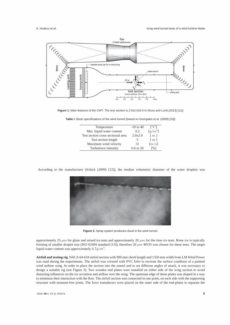
A. Hudecz et.al. Icing wind tunnel tests of a wind turbine blade
Figure 1. Main features of the CWT. The test section is 2.0x2.0x5.0 m (Koss and Lund (2013) [11])
Table I. Basic specifications of the wind tunnel (based on Georgakis et al. (2009) [10])
Temperature -10 to 40 [oC]Min. liquid water content 0.2 [g/m3]
Test section cross-sectional area 2.0x2.0 [ m ]Test section length 5 [ m ]
Maximum wind velocity 31 [m/s]Turbulence intensity 0.6 to 20 [%]
According to the manufacturer (Schick (2009) [12]), the median volumetric diameter of the water droplets was
Figure 2. Spray system produces cloud in the wind tunnel.
approximately 25 μm for glaze and mixed ice tests and approximately 20 μm for the rime ice tests. Rime ice is typicallyforming of smaller droplet size (ISO 62494 standard [13]), therefore 20 μm MVD was chosen for these tests. The targetliquid water content was approximately 0.7g/m3.
Airfoil and testing rig. NACA 64-618 airfoil section with 900 mm chord length and 1350 mm width from LM Wind Powerwas used during the experiments. The airfoil was covered with PVC folio to recreate the surface condition of a paintedwind turbine wing. In order to place the section into the tunnel and to set different angles of attack, it was necessary todesign a suitable rig (see Figure 3). Two wooden end plates were installed on either side of the wing section to avoiddistorting influences on the ice accretion and airflow over the wing. The upstream edge of these plates was shaped in a wayto minimize their interaction with the flow. The airfoil section was connected in one point, on each side with the supportingstructure with moment-free joints. The force transducers were placed on the outer side of the end-plates to separate the
2010; 00:1–14 c© 2010 & 3
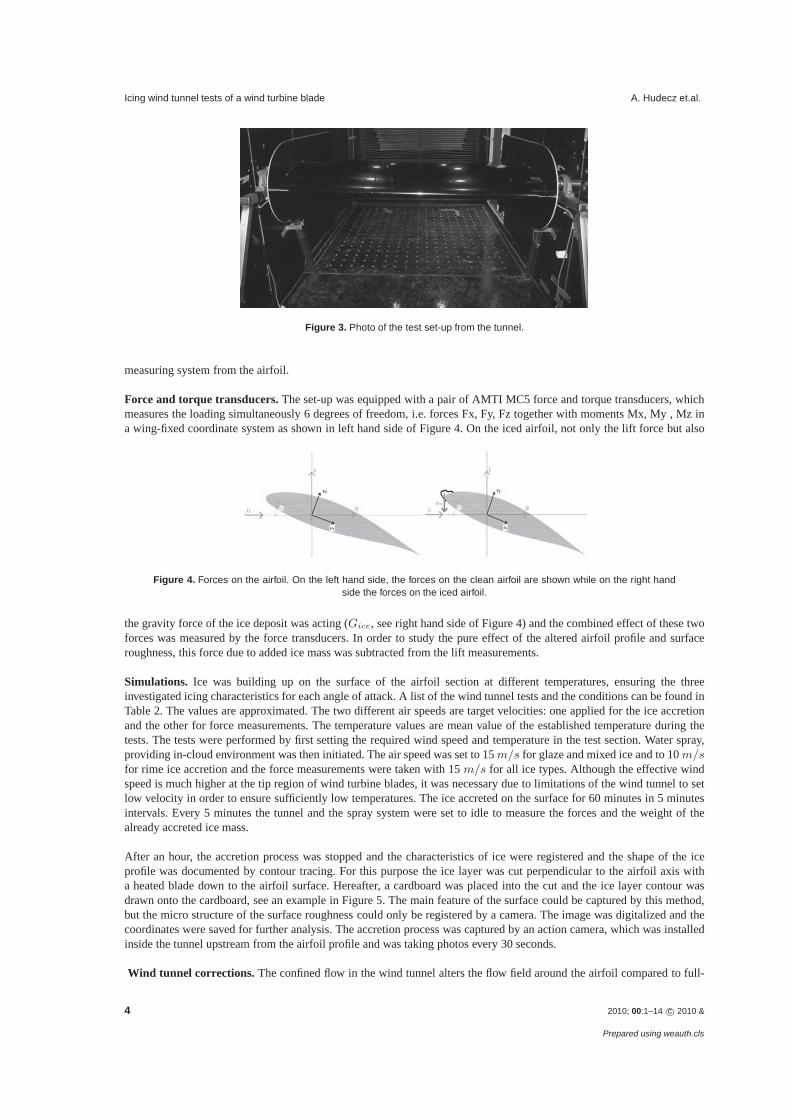
Icing wind tunnel tests of a wind turbine blade A. Hudecz et.al.
Figure 3. Photo of the test set-up from the tunnel.
measuring system from the airfoil.
Force and torque transducers. The set-up was equipped with a pair of AMTI MC5 force and torque transducers, whichmeasures the loading simultaneously 6 degrees of freedom, i.e. forces Fx, Fy, Fz together with moments Mx, My , Mz ina wing-fixed coordinate system as shown in left hand side of Figure 4. On the iced airfoil, not only the lift force but also
Figure 4. Forces on the airfoil. On the left hand side, the forces on the clean airfoil are shown while on the right handside the forces on the iced airfoil.
the gravity force of the ice deposit was acting (Gice, see right hand side of Figure 4) and the combined effect of these twoforces was measured by the force transducers. In order to study the pure effect of the altered airfoil profile and surfaceroughness, this force due to added ice mass was subtracted from the lift measurements.
Simulations. Ice was building up on the surface of the airfoil section at different temperatures, ensuring the threeinvestigated icing characteristics for each angle of attack. A list of the wind tunnel tests and the conditions can be found inTable 2. The values are approximated. The two different air speeds are target velocities: one applied for the ice accretionand the other for force measurements. The temperature values are mean value of the established temperature during thetests. The tests were performed by first setting the required wind speed and temperature in the test section. Water spray,providing in-cloud environment was then initiated. The air speed was set to 15 m/s for glaze and mixed ice and to 10 m/sfor rime ice accretion and the force measurements were taken with 15 m/s for all ice types. Although the effective windspeed is much higher at the tip region of wind turbine blades, it was necessary due to limitations of the wind tunnel to setlow velocity in order to ensure sufficiently low temperatures. The ice accreted on the surface for 60 minutes in 5 minutesintervals. Every 5 minutes the tunnel and the spray system were set to idle to measure the forces and the weight of thealready accreted ice mass.
After an hour, the accretion process was stopped and the characteristics of ice were registered and the shape of the iceprofile was documented by contour tracing. For this purpose the ice layer was cut perpendicular to the airfoil axis witha heated blade down to the airfoil surface. Hereafter, a cardboard was placed into the cut and the ice layer contour wasdrawn onto the cardboard, see an example in Figure 5. The main feature of the surface could be captured by this method,but the micro structure of the surface roughness could only be registered by a camera. The image was digitalized and thecoordinates were saved for further analysis. The accretion process was captured by an action camera, which was installedinside the tunnel upstream from the airfoil profile and was taking photos every 30 seconds.
Wind tunnel corrections. The confined flow in the wind tunnel alters the flow field around the airfoil compared to full-
4 2010; 00:1–14 c© 2010 &
Prepared using weauth.cls
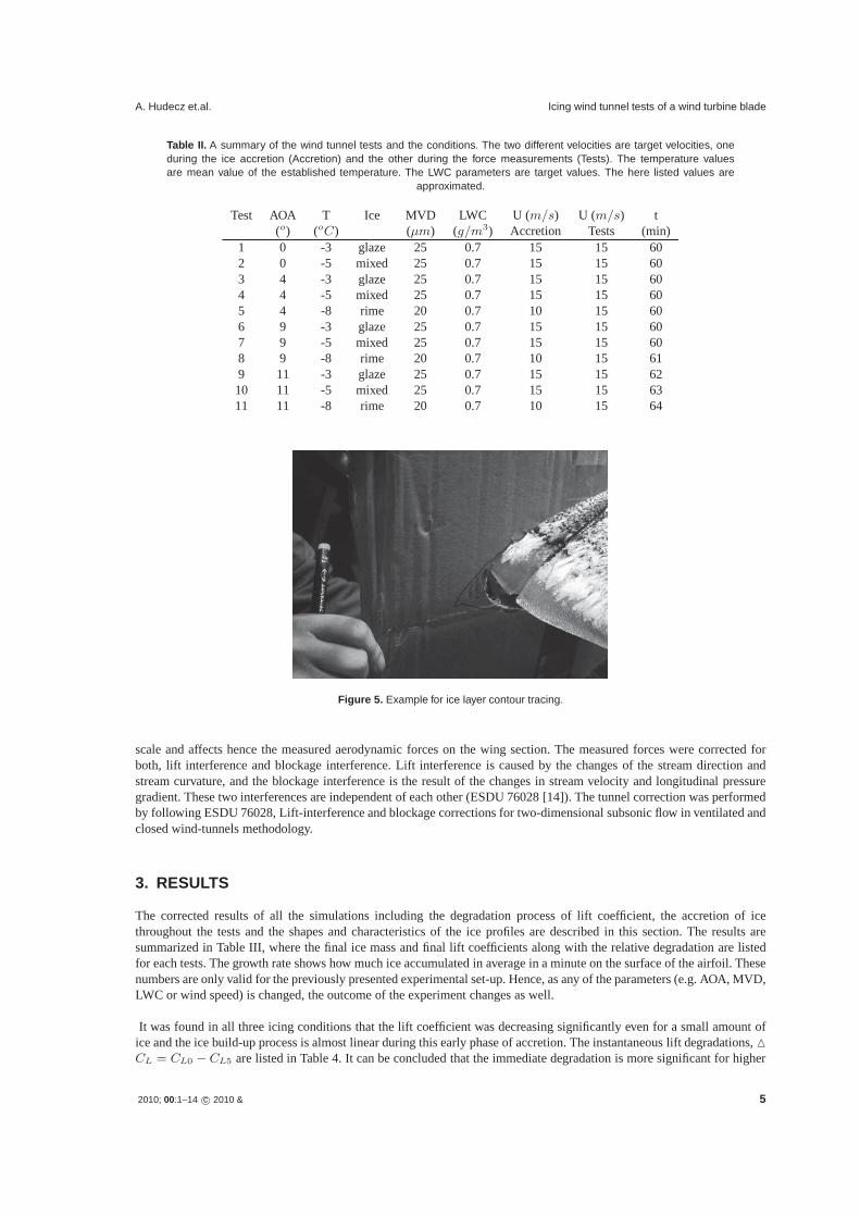
A. Hudecz et.al. Icing wind tunnel tests of a wind turbine blade
Table II. A summary of the wind tunnel tests and the conditions. The two different velocities are target velocities, oneduring the ice accretion (Accretion) and the other during the force measurements (Tests). The temperature valuesare mean value of the established temperature. The LWC parameters are target values. The here listed values are
approximated.
Test AOA T Ice MVD LWC U (m/s) U (m/s) t(o) (oC) (μm) (g/m3) Accretion Tests (min)
1 0 -3 glaze 25 0.7 15 15 602 0 -5 mixed 25 0.7 15 15 603 4 -3 glaze 25 0.7 15 15 604 4 -5 mixed 25 0.7 15 15 605 4 -8 rime 20 0.7 10 15 606 9 -3 glaze 25 0.7 15 15 607 9 -5 mixed 25 0.7 15 15 608 9 -8 rime 20 0.7 10 15 619 11 -3 glaze 25 0.7 15 15 6210 11 -5 mixed 25 0.7 15 15 6311 11 -8 rime 20 0.7 10 15 64
Figure 5. Example for ice layer contour tracing.
scale and affects hence the measured aerodynamic forces on the wing section. The measured forces were corrected forboth, lift interference and blockage interference. Lift interference is caused by the changes of the stream direction andstream curvature, and the blockage interference is the result of the changes in stream velocity and longitudinal pressuregradient. These two interferences are independent of each other (ESDU 76028 [14]). The tunnel correction was performedby following ESDU 76028, Lift-interference and blockage corrections for two-dimensional subsonic flow in ventilated andclosed wind-tunnels methodology.
3. RESULTS
The corrected results of all the simulations including the degradation process of lift coefficient, the accretion of icethroughout the tests and the shapes and characteristics of the ice profiles are described in this section. The results aresummarized in Table III, where the final ice mass and final lift coefficients along with the relative degradation are listedfor each tests. The growth rate shows how much ice accumulated in average in a minute on the surface of the airfoil. Thesenumbers are only valid for the previously presented experimental set-up. Hence, as any of the parameters (e.g. AOA, MVD,LWC or wind speed) is changed, the outcome of the experiment changes as well.
It was found in all three icing conditions that the lift coefficient was decreasing significantly even for a small amount ofice and the ice build-up process is almost linear during this early phase of accretion. The instantaneous lift degradations, �CL = CL0 −CL5 are listed in Table 4. It can be concluded that the immediate degradation is more significant for higher
2010; 00:1–14 c© 2010 & 5
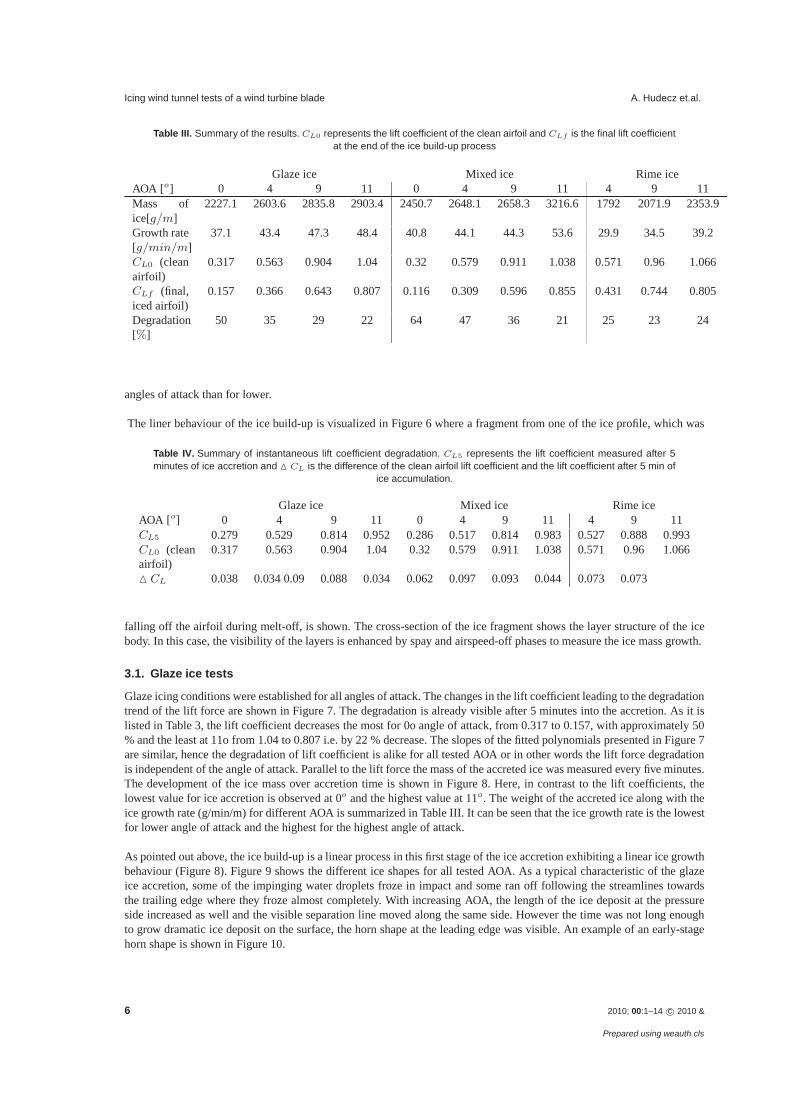
Icing wind tunnel tests of a wind turbine blade A. Hudecz et.al.
Table III. Summary of the results. CL0 represents the lift coefficient of the clean airfoil and CLf is the final lift coefficientat the end of the ice build-up process
Glaze ice Mixed ice Rime iceAOA [o] 0 4 9 11 0 4 9 11 4 9 11Mass ofice[g/m]
2227.1 2603.6 2835.8 2903.4 2450.7 2648.1 2658.3 3216.6 1792 2071.9 2353.9
Growth rate[g/min/m]
37.1 43.4 47.3 48.4 40.8 44.1 44.3 53.6 29.9 34.5 39.2
CL0 (cleanairfoil)
0.317 0.563 0.904 1.04 0.32 0.579 0.911 1.038 0.571 0.96 1.066
CLf (final,iced airfoil)
0.157 0.366 0.643 0.807 0.116 0.309 0.596 0.855 0.431 0.744 0.805
Degradation[%]
50 35 29 22 64 47 36 21 25 23 24
angles of attack than for lower.
The liner behaviour of the ice build-up is visualized in Figure 6 where a fragment from one of the ice profile, which was
Table IV. Summary of instantaneous lift coefficient degradation. CL5 represents the lift coefficient measured after 5minutes of ice accretion and � CL is the difference of the clean airfoil lift coefficient and the lift coefficient after 5 min of
ice accumulation.
Glaze ice Mixed ice Rime iceAOA [o] 0 4 9 11 0 4 9 11 4 9 11CL5 0.279 0.529 0.814 0.952 0.286 0.517 0.814 0.983 0.527 0.888 0.993CL0 (cleanairfoil)
0.317 0.563 0.904 1.04 0.32 0.579 0.911 1.038 0.571 0.96 1.066
� CL 0.038 0.034 0.09 0.088 0.034 0.062 0.097 0.093 0.044 0.073 0.073
falling off the airfoil during melt-off, is shown. The cross-section of the ice fragment shows the layer structure of the icebody. In this case, the visibility of the layers is enhanced by spay and airspeed-off phases to measure the ice mass growth.
3.1. Glaze ice tests
Glaze icing conditions were established for all angles of attack. The changes in the lift coefficient leading to the degradationtrend of the lift force are shown in Figure 7. The degradation is already visible after 5 minutes into the accretion. As it islisted in Table 3, the lift coefficient decreases the most for 0o angle of attack, from 0.317 to 0.157, with approximately 50% and the least at 11o from 1.04 to 0.807 i.e. by 22 % decrease. The slopes of the fitted polynomials presented in Figure 7are similar, hence the degradation of lift coefficient is alike for all tested AOA or in other words the lift force degradationis independent of the angle of attack. Parallel to the lift force the mass of the accreted ice was measured every five minutes.The development of the ice mass over accretion time is shown in Figure 8. Here, in contrast to the lift coefficients, thelowest value for ice accretion is observed at 0o and the highest value at 11o. The weight of the accreted ice along with theice growth rate (g/min/m) for different AOA is summarized in Table III. It can be seen that the ice growth rate is the lowestfor lower angle of attack and the highest for the highest angle of attack.
As pointed out above, the ice build-up is a linear process in this first stage of the ice accretion exhibiting a linear ice growthbehaviour (Figure 8). Figure 9 shows the different ice shapes for all tested AOA. As a typical characteristic of the glazeice accretion, some of the impinging water droplets froze in impact and some ran off following the streamlines towardsthe trailing edge where they froze almost completely. With increasing AOA, the length of the ice deposit at the pressureside increased as well and the visible separation line moved along the same side. However the time was not long enoughto grow dramatic ice deposit on the surface, the horn shape at the leading edge was visible. An example of an early-stagehorn shape is shown in Figure 10.
6 2010; 00:1–14 c© 2010 &
Prepared using weauth.cls
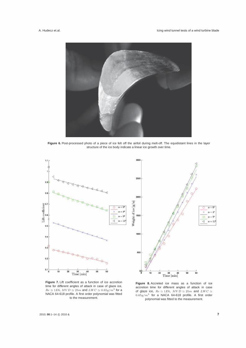
A. Hudecz et.al. Icing wind tunnel tests of a wind turbine blade
Figure 6. Post-processed photo of a piece of ice felt off the airfoil during melt-off. The equidistant lines in the layerstructure of the ice body indicate a linear ice growth over time.
Figure 7. Lift coefficient as a function of ice accretiontime for different angles of attack in case of glaze ice,Re � 1E6, MV D � 25m and LWC � 0.65g/m3 for aNACA 64-618 profile. A first order polynomial was fitted
to the measurement.
Figure 8. Accreted ice mass as a function of iceaccretion time for different angles of attack in caseof glaze ice, Re � 1E6, MV D � 25m and LWC �
0.65g/m3 for a NACA 64-618 profile. A first orderpolynomial was fitted to the measurement.
2010; 00:1–14 c© 2010 & 7
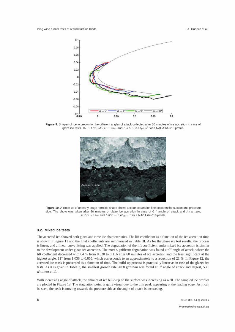
Icing wind tunnel tests of a wind turbine blade A. Hudecz et.al.
Figure 9. Shapes of ice accretion for the different angles of attack collected after 60 minutes of ice accretion in case ofglaze ice tests, Re � 1E6, MV D � 25m and LWC � 0.65g/m3 for a NACA 64-618 profile.
Figure 10. A close-up of an early-stage horn ice shape shows a clear separation line between the suction and pressureside. The photo was taken after 60 minutes of glaze ice accretion in case of 0 o angle of attack and Re � 1E6,
MV D � 25m and LWC � 0.65g/m3 for a NACA 64-618 profile.
3.2. Mixed ice tests
The accreted ice showed both glaze and rime ice characteristics. The lift coefficient as a function of the ice accretion timeis shown in Figure 11 and the final coefficients are summarized in Table III. As for the glaze ice test results, the processis linear, and a linear curve fitting was applied. The degradation of the lift coefficient under mixed ice accretion is similarto the development under glaze ice accretion. The most significant degradation was found at 0o angle of attack, where thelift coefficient decreased with 64 % from 0.320 to 0.116 after 60 minutes of ice accretion and the least significant at thehighest angle, 11o from 1.038 to 0.855, which corresponds to an approximately to a reduction of 21 %. In Figure 12, theaccreted ice mass is presented as a function of time. The build-up process is practically linear as in case of the glazes icetests. As it is given in Table 3, the smallest growth rate, 40.8 g/min/m was found at 0o angle of attack and largest, 53.6g/min/m at 11o.
With increasing angle of attack, the amount of ice build-up on the surface was increasing as well. The sampled ice profilesare plotted in Figure 13. The stagnation point is quite visual due to the thin peak appearing at the leading edge. As it canbe seen, the peak is moving towards the pressure side as the angle of attack is increasing.
8 2010; 00:1–14 c© 2010 &
Prepared using weauth.cls
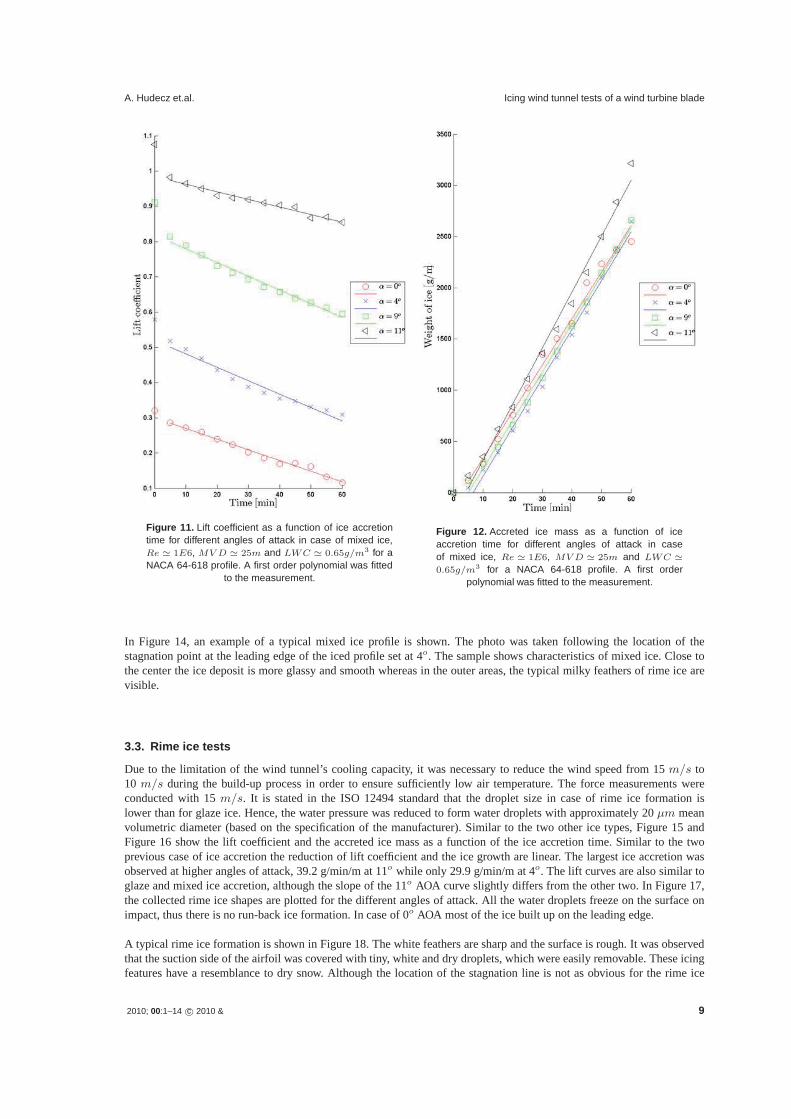
A. Hudecz et.al. Icing wind tunnel tests of a wind turbine blade
Figure 11. Lift coefficient as a function of ice accretiontime for different angles of attack in case of mixed ice,Re � 1E6, MV D � 25m and LWC � 0.65g/m3 for aNACA 64-618 profile. A first order polynomial was fitted
to the measurement.
Figure 12. Accreted ice mass as a function of iceaccretion time for different angles of attack in caseof mixed ice, Re � 1E6, MV D � 25m and LWC �
0.65g/m3 for a NACA 64-618 profile. A first orderpolynomial was fitted to the measurement.
In Figure 14, an example of a typical mixed ice profile is shown. The photo was taken following the location of thestagnation point at the leading edge of the iced profile set at 4o. The sample shows characteristics of mixed ice. Close tothe center the ice deposit is more glassy and smooth whereas in the outer areas, the typical milky feathers of rime ice arevisible.
3.3. Rime ice tests
Due to the limitation of the wind tunnel’s cooling capacity, it was necessary to reduce the wind speed from 15 m/s to10 m/s during the build-up process in order to ensure sufficiently low air temperature. The force measurements wereconducted with 15 m/s. It is stated in the ISO 12494 standard that the droplet size in case of rime ice formation islower than for glaze ice. Hence, the water pressure was reduced to form water droplets with approximately 20 μm meanvolumetric diameter (based on the specification of the manufacturer). Similar to the two other ice types, Figure 15 andFigure 16 show the lift coefficient and the accreted ice mass as a function of the ice accretion time. Similar to the twoprevious case of ice accretion the reduction of lift coefficient and the ice growth are linear. The largest ice accretion wasobserved at higher angles of attack, 39.2 g/min/m at 11o while only 29.9 g/min/m at 4o. The lift curves are also similar toglaze and mixed ice accretion, although the slope of the 11o AOA curve slightly differs from the other two. In Figure 17,the collected rime ice shapes are plotted for the different angles of attack. All the water droplets freeze on the surface onimpact, thus there is no run-back ice formation. In case of 0o AOA most of the ice built up on the leading edge.
A typical rime ice formation is shown in Figure 18. The white feathers are sharp and the surface is rough. It was observedthat the suction side of the airfoil was covered with tiny, white and dry droplets, which were easily removable. These icingfeatures have a resemblance to dry snow. Although the location of the stagnation line is not as obvious for the rime ice
2010; 00:1–14 c© 2010 & 9
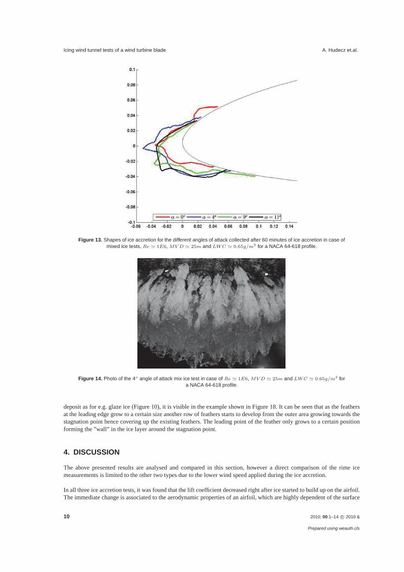
Icing wind tunnel tests of a wind turbine blade A. Hudecz et.al.
Figure 13. Shapes of ice accretion for the different angles of attack collected after 60 minutes of ice accretion in case ofmixed ice tests, Re � 1E6, MV D � 25m and LWC � 0.65g/m3 for a NACA 64-618 profile.
Figure 14. Photo of the 4o angle of attack mix ice test in case of Re � 1E6, MV D � 25m and LWC � 0.65g/m3 fora NACA 64-618 profile.
deposit as for e.g. glaze ice (Figure 10), it is visible in the example shown in Figure 18. It can be seen that as the feathersat the leading edge grow to a certain size another row of feathers starts to develop from the outer area growing towards thestagnation point hence covering up the existing feathers. The leading point of the feather only grows to a certain positionforming the ”wall” in the ice layer around the stagnation point.
4. DISCUSSION
The above presented results are analysed and compared in this section, however a direct comparison of the rime icemeasurements is limited to the other two types due to the lower wind speed applied during the ice accretion.
In all three ice accretion tests, it was found that the lift coefficient decreased right after ice started to build up on the airfoil.The immediate change is associated to the aerodynamic properties of an airfoil, which are highly dependent of the surface
10 2010; 00:1–14 c© 2010 &
Prepared using weauth.cls
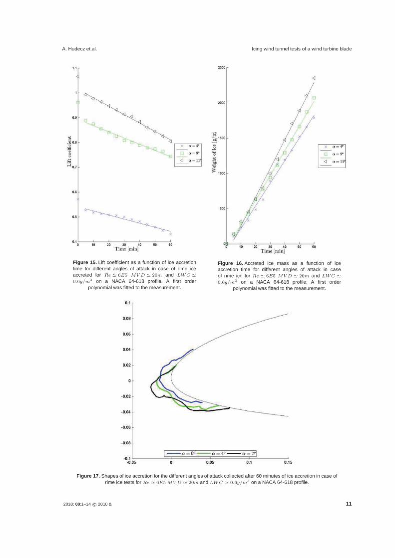
A. Hudecz et.al. Icing wind tunnel tests of a wind turbine blade
Figure 15. Lift coefficient as a function of ice accretiontime for different angles of attack in case of rime iceaccreted for Re � 6E5 MV D � 20m and LWC �
0.6g/m3 on a NACA 64-618 profile. A first orderpolynomial was fitted to the measurement.
Figure 16. Accreted ice mass as a function of iceaccretion time for different angles of attack in caseof rime ice for Re � 6E5 MV D � 20m and LWC �
0.6g/m3 on a NACA 64-618 profile. A first orderpolynomial was fitted to the measurement.
Figure 17. Shapes of ice accretion for the different angles of attack collected after 60 minutes of ice accretion in case ofrime ice tests for Re � 6E5 MV D � 20m and LWC � 0.6g/m3 on a NACA 64-618 profile.
2010; 00:1–14 c© 2010 & 11
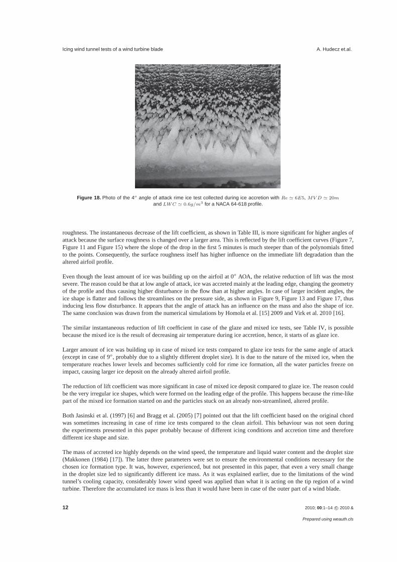
Icing wind tunnel tests of a wind turbine blade A. Hudecz et.al.
Figure 18. Photo of the 4o angle of attack rime ice test collected during ice accretion with Re � 6E5, MV D � 20m
and LWC � 0.6g/m3 for a NACA 64-618 profile.
roughness. The instantaneous decrease of the lift coefficient, as shown in Table III, is more significant for higher angles ofattack because the surface roughness is changed over a larger area. This is reflected by the lift coefficient curves (Figure 7,Figure 11 and Figure 15) where the slope of the drop in the first 5 minutes is much steeper than of the polynomials fittedto the points. Consequently, the surface roughness itself has higher influence on the immediate lift degradation than thealtered airfoil profile.
Even though the least amount of ice was building up on the airfoil at 0o AOA, the relative reduction of lift was the mostsevere. The reason could be that at low angle of attack, ice was accreted mainly at the leading edge, changing the geometryof the profile and thus causing higher disturbance in the flow than at higher angles. In case of larger incident angles, theice shape is flatter and follows the streamlines on the pressure side, as shown in Figure 9, Figure 13 and Figure 17, thusinducing less flow disturbance. It appears that the angle of attack has an influence on the mass and also the shape of ice.The same conclusion was drawn from the numerical simulations by Homola et al. [15] 2009 and Virk et al. 2010 [16].
The similar instantaneous reduction of lift coefficient in case of the glaze and mixed ice tests, see Table IV, is possiblebecause the mixed ice is the result of decreasing air temperature during ice accretion, hence, it starts of as glaze ice.
Larger amount of ice was building up in case of mixed ice tests compared to glaze ice tests for the same angle of attack(except in case of 9o, probably due to a slightly different droplet size). It is due to the nature of the mixed ice, when thetemperature reaches lower levels and becomes sufficiently cold for rime ice formation, all the water particles freeze onimpact, causing larger ice deposit on the already altered airfoil profile.
The reduction of lift coefficient was more significant in case of mixed ice deposit compared to glaze ice. The reason couldbe the very irregular ice shapes, which were formed on the leading edge of the profile. This happens because the rime-likepart of the mixed ice formation started on and the particles stuck on an already non-streamlined, altered profile.
Both Jasinski et al. (1997) [6] and Bragg et al. (2005) [7] pointed out that the lift coefficient based on the original chordwas sometimes increasing in case of rime ice tests compared to the clean airfoil. This behaviour was not seen duringthe experiments presented in this paper probably because of different icing conditions and accretion time and thereforedifferent ice shape and size.
The mass of accreted ice highly depends on the wind speed, the temperature and liquid water content and the droplet size(Makkonen (1984) [17]). The latter three parameters were set to ensure the environmental conditions necessary for thechosen ice formation type. It was, however, experienced, but not presented in this paper, that even a very small changein the droplet size led to significantly different ice mass. As it was explained earlier, due to the limitations of the windtunnel’s cooling capacity, considerably lower wind speed was applied than what it is acting on the tip region of a windturbine. Therefore the accumulated ice mass is less than it would have been in case of the outer part of a wind blade.
12 2010; 00:1–14 c© 2010 &
Prepared using weauth.cls

A. Hudecz et.al. Icing wind tunnel tests of a wind turbine blade
Although the physical characteristics of the ice deposits were similar to the one published in other studies e.g. Bose (1992)[18] and ISO 12494 [13] standard, some differences were observed. In case of glaze ice deposits, as it can be seen in Figure10, the ice deposit consists of small beads. It was seen during the experiments that the water droplets, which did not freezeon the surface on impact, formed small beads before they eventually ran off. Every 5 minutes, the tunnel and the spraysystem was set to idle for approximately one and a half minutes in order to measure the weight of the accreted ice mass.Even though this period is short, it could provide just enough time to get these water beads to freeze.
In case of the mixed ice tests, the observed peak at the stagnation point in Figure 13 could probably be formed due to thestatic feature of the tests. These peaks are not experienced or have been reported yet in case of an actual rotating windturbine blade. Due to atmospheric turbulence, wind shear and tower passage, the angle of attack is varying in time arounda mean value on a wind turbine blade which will give a broader ice accretion at the leading edge since the stagnation pointis not constant.
5. CONCLUSION
In this paper, the results of a series of experiments on a NACA 64-618 profile in a climatic wind tunnel were presented.There were a number of tests performed at different angles of attack and temperature in order to monitor the alteration ofthe lift coefficient and thus the lift force along with the weight of accumulated ice throughout the first 60 minutes of iceaccretion under controlled conditions. It was seen that both the ice accretion and the degradation shows a linear trend. Thealteration of the surface roughness has a more significant effect on the initial lift coefficient than the shape of the changedairfoil profile. As the angle of attack increased the larger the degradation of the instantaneous lift coefficient got.
It was also found, that not only the temperature, but the angle of attack has an influence on the mass and also the shape ofice deposit. Even though the least amount of ice was building up on the airfoil at low angles of attack, the relative reductionwas the most severe in these cases, thus the higher the angle of attack the lower the lift coefficient degradation.
More ice built up on the airfoil during the mixed ice tests than the glaze ice tests and hence causing more significant liftcoefficient degradation.
ACKNOWLEDGMENT
Force Technology and LM Wind Power are acknowledged for allowing us to use their unique facility to conduct the testsand for lending the NACA 64-618 profile, respectively.
REFERENCES
1. Tammelin B, Cavaliere M, Holttinen H, Morgan C, Seifert H. and Santti K. Wind energy production in cold climate(WECO). Technical report, Finnish Meteorological Institute, 1998.
2. Tallhaug L, Ronsten G, Horbaty R, Cattin R, Laakso T, Durstewitz M, Lacroix A, Peltola E, and Wallenius T. Windenergy projects in cold climate. Technical report, Executive Committee of the International Energy Agency Programmefor Research and Development on Wind Energy Conversion Systems, 2009.
3. Baring-Gould I, Cattin R, Durstewitz M, Hulkkonen M, Krenn A, Laakso T, Lacroix A, Peltola E, Ronsten G, TallhaugL, and Wallenius T. 13. Wind Energy Projects in Cold Climates. Technical report, 2011.
4. Lynch F. T. and Khodadoust A. Effects of ice accretions on aircraft aerodynamics. Progress in Aerospace Sciences2001, 37(8):669-767.
5. Seifert H. and Richert F. Aerodynamics of iced airfoils and their influence on loads and power production. EuropeanWind Energy Conference, 1997.
6. Jasinski W. J, Noe S. C, Selig M. S, and Bragg M. B. Wind turbine performance under icing conditions. Journal ofSolar Energy Engineering 1997, ASME, 120(1):60-65.
7. Bragg M, Broeren A. P, and Blumenthal L. Iced-airfoil aerodynamics. Progress in Aerospace Sciences 2005,41(5):323-362.
8. Hochart C, Fortin G, and Perron J. Wind turbine performance under icing conditions. Wind Energy 2008, 11:319333.9. Addy H. E, Broeren A. P, Zoeckler J. G, and Lee S. A Wind Tunnel Study of Icing Effects on a Business Jet Airfoil. In:
American Institute of Aeronautics and Astronautics, 41. Aerospace Sciences Meeting and Exhibit, 2003.
2010; 00:1–14 c© 2010 & 13

Icing wind tunnel tests of a wind turbine blade A. Hudecz et.al.
10. Georgakis C, Koss H, and Ricciardelli F. Design specifications for a novel climatic wind tunnel for the testing ofstructural cables. International Symposium on Cable Dynamics (ISCD) - 8, 2009, Paris, France.
11. Koss H. H. and Lund M. S. M. Experimental Investigation of Aerodynamic Instability of Iced Bridge Cable Sections.In: 6th European and African Conference on Wind Engineering, Cambridge, UK, 2013
12. Schick R. J. Spray technology reference guide: Understanding drop size, bulletin 459c. Technical report, SprayingSystems Co.
13. ISO 12494. Atmospheric icing of structures. Technical report, ISO Copyright Office, Geneva, Switzerland, 2001.14. ESDU 76028, Lift-Interference and Blockage Corrections for Two-Dimensional Subsonic Flow in Ventilated and
Closed Wind Tunnel, ESDU 1976.15. Homola M. C, Wallenius T, Makkonen L, and Nicklasson P. J. The relationship between chord length and rime icing
on wind turbines. Wind Energy 2009, 13(7):627-632.16. Virk M. S, Homola M. C, Nicklasson P. J. Effect of Rime Ice Accretion on Aerodynamic Characteristics of Wind
Turbine Blade Profiles. Wind Engineering 2010, 34 (2):207-218.17. Makkonen L. Atmospheric Icing on Sea Structure. U.S. Army Cold Regions Research and Engineering Laboratory,
Hanover, New Hampshire, 1984.18. Bose N. Icing on a small horizontal-axis wind turbine - Part 1: Glaze ice profiles. Journal of Wind Engineering and
Industrial Aerodynamics 1992, 45:7585.
14 2010; 00:1–14 c© 2010 &
Prepared using weauth.cls
IWAIS XV, St. John’s, Newfoundland and Labrador, Canada, September 8-11, 2013
Abstract — In this paper, both experimental and numerical
simulations of the effects of ice accretion on a NACA 64-618 airfoil section with 7o angle of attack are presented. The wind tunnel tests were conducted in a closed-circuit climatic wind tunnel at Force Technology in Denmark. The changes of aerodynamic forces were monitored as ice was building up on the airfoil for glaze, rime and mixed ice. In the first part of the numerical analysis, the resulted ice profiles of the wind tunnel tests were compared to profiles estimated by using the 2D ice accretion code TURBICE. In the second part, Ansys Fluent was used to estimate the aerodynamic coefficients of the iced profiles. It was found that both reduction of lift coefficient and increase of drag coefficient is a nearly linear process. Mixed ice formation causes the largest flow disturbance and thus the most lift degradation. Whereas, the suction side of the rime iced ice profile follows the streamlines quite well, disturbing the flow the least. The TURBICE analysis agrees fairly with the profiles produced during the wind tunnel testing.
I. INTRODUCTION In cold climate areas with temperatures below 0oC and humid environment for larger periods of the year icing represents an significant threat to the performance and durability of wind turbines (Tammelin et al. [1], Tallhaug et al. [2] and Baring-Gould et al. [3]). In this paper, both experimental and numerical simulations of the effects of ice accretion on a NACA 64-618 airfoil section are presented. The experiments were performed in a closed-circuit climatic wind tunnel at FORCE Technology in Denmark. Aerodynamic forces were monitored throughout the icing process for 7o angle of attack at different temperatures, which were used to ensure adequate environment for the typical ice types, rime, glaze and mixed ice, which threaten the operation of wind turbine. There were already a number of wind tunnel tests conducted on iced airfoils in the past. Seifert and Richert [4] and Jasinski et al. [5] used artificial ice deposits during their experiments. In case of Seifert and Richert’s tests [4], the molds were made of actual ice fragments from a wind turbine, whereas Jasinski et al. [5] simulated the ice profiles with Nasa’s ice accretion code, LEWICE. Hochart et al. [6] performed two-phase experiments. In the first phase, the ice deposit was grown and then in the second phase, efficiency tests were performed. The
main difference from these tests and the ones presented in this paper is the fact that the aerodynamic forces were monitored as ice was accumulating. At the end of the tests, the ice profiles were documented by contour tracing for further, numerical analysis.
In the recent years, especially due to the increased computer power, it became possible to determine the performance of iced wind turbine much faster and more accurately with computational fluid dynamics (CFD) and panel method based models. Homola et al. [7] have used a two-steps method, combining TURBICE and Ansys Fluent to investigate the effect of ice similarly on a NACA 64-618 profile. TURBICE is comprehensive numerical ice accretion software from VTT, Technical Research Centre of Finland, which uses panel method to calculate the potential flow. It was verified by icing wind tunnel testing of both aircraft and wind turbine airfoils. The accuracy of the solution is dependent on the number of the panels and their distribution around the section (Makkonen et al., [8]). Homola et al. [7] found that the lift coefficient was reduced in all cases and the smallest change was observed in case of rime ice. During the CFD simulations, it was found that the horn type glaze ice shape causes the largest separation, which leads to a significantly reduced lift and higher drag coefficient.
Etemaddar et al. [9] has also used the same profile in their numerical analysis. In their study, they combined Nasa’s LEWICE code with Ansys Fluent and pointed out that the ice load increases with liquid water content (LWC), median volumetric diameter (MVD) and relative wind speed.
The numerical simulations presented in this paper were carried out in two parts. First, the collected ice profiles were compared to profiles generated in TURBICE. In the second part, numerical analyses were done on the iced profiles from the wind tunnel tests in Ansys Fluent.
The aim of the wind tunnel tests was to investigate the changes of aerodynamics as ice built up on the airfoil for glaze, rime and mixed ice tests. The relative changes of lift and drag coefficients along with the shape of the ice deposits could be compared to results of the numerical analysis.
Ice Accretion on Wind Turbine Blades Adriána Hudecz#1, Holger Koss *2, Martin O. L. Hansen #†3 #Department of Wind Energy, Technical University of Denmark
1 [email protected] 3 [email protected]
*Department of Civil Engineering, Technical University of Denmark 2 [email protected]
†Centre for Ships and Ocean Structures, Department of Marine Technology, Norwegian University of Science and Technology
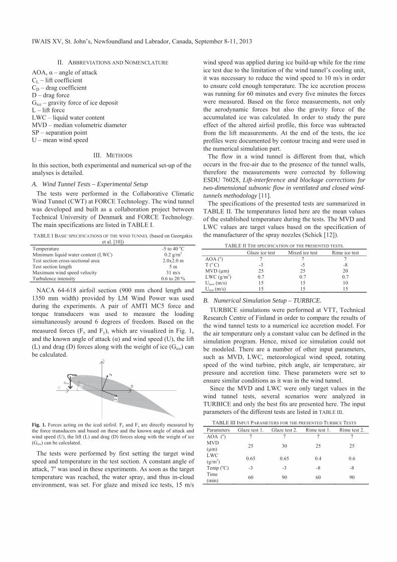
IWAIS XV, St. John’s, Newfoundland and Labrador, Canada, September 8-11, 2013
II. ABBREVIATIONS AND NOMENCLATURE AOA, – angle of attack CL – lift coefficient CD – drag coefficient D – drag force Gice – gravity force of ice deposit L – lift force LWC – liquid water content MVD – median volumetric diameter SP – separation point U – mean wind speed
III. METHODS In this section, both experimental and numerical set-up of the analyses is detailed.
A. Wind Tunnel Tests – Experimental Setup The tests were performed in the Collaborative Climatic
Wind Tunnel (CWT) at FORCE Technology. The wind tunnel was developed and built as a collaboration project between Technical University of Denmark and FORCE Technology. The main specifications are listed in TABLE I. TABLE I BASIC SPECIFICATIONS OF THE WIND TUNNEL (based on Georgakis
et al. [10]) Temperature -5 to 40 oC Minimum liquid water content (LWC) 0.2 g/m3 Test section cross-sectional area 2.0x2.0 m Test section length 5 m Maximum wind speed velocity 31 m/s Turbulence intensity 0.6 to 20 %
NACA 64-618 airfoil section (900 mm chord length and 1350 mm width) provided by LM Wind Power was used during the experiments. A pair of AMTI MC5 force and torque transducers was used to measure the loading simultaneously around 6 degrees of freedom. Based on the measured forces (Fx and Fy), which are visualized in Fig. 1, and the known angle of attack ( ) and wind speed (U), the lift (L) and drag (D) forces along with the weight of ice (Gice) can be calculated.
Fig. 1. Forces acting on the iced airfoil. Fy and Fx are directly measured by the force transducers and based on these and the known angle of attack and wind speed (U), the lift (L) and drag (D) forces along with the weight of ice (Gice) can be calculated.
The tests were performed by first setting the target wind speed and temperature in the test section. A constant angle of attack, 7o was used in these experiments. As soon as the target temperature was reached, the water spray, and thus in-cloud environment, was set. For glaze and mixed ice tests, 15 m/s
wind speed was applied during ice build-up while for the rime ice test due to the limitation of the wind tunnel’s cooling unit, it was necessary to reduce the wind speed to 10 m/s in order to ensure cold enough temperature. The ice accretion process was running for 60 minutes and every five minutes the forces were measured. Based on the force measurements, not only the aerodynamic forces but also the gravity force of the accumulated ice was calculated. In order to study the pure effect of the altered airfoil profile, this force was subtracted from the lift measurements. At the end of the tests, the ice profiles were documented by contour tracing and were used in the numerical simulation part.
The flow in a wind tunnel is different from that, which occurs in the free-air due to the presence of the tunnel walls, therefore the measurements were corrected by following ESDU 76028, Lift-interference and blockage corrections for two-dimensional subsonic flow in ventilated and closed wind-tunnels methodology [11].
The specifications of the presented tests are summarized in TABLE II. The temperatures listed here are the mean values of the established temperature during the tests. The MVD and LWC values are target values based on the specification of the manufacturer of the spray nozzles (Schick [12]).
TABLE II THE SPECIFICATION OF THE PRESENTED TESTS. Glaze ice test Mixed ice test Rime ice test
AOA (o) 7 7 7 T (o C) -3 -5 -8 MVD (μm) 25 25 20 LWC (g/m3) 0.7 0.7 0.7 Uaccr (m/s) 15 15 10 Utest (m/s) 15 15 15
B. Numerical Simulation Setup – TURBICE. TURBICE simulations were performed at VTT, Technical
Research Centre of Finland in order to compare the results of the wind tunnel tests to a numerical ice accretion model. For the air temperature only a constant value can be defined in the simulation program. Hence, mixed ice simulation could not be modeled. There are a number of other input parameters, such as MVD, LWC, meteorological wind speed, rotating speed of the wind turbine, pitch angle, air temperature, air pressure and accretion time. These parameters were set to ensure similar conditions as it was in the wind tunnel.
Since the MVD and LWC were only target values in the wind tunnel tests, several scenarios were analyzed in TURBICE and only the best fits are presented here. The input parameters of the different tests are listed in TABLE III.
TABLE III INPUT PARAMETERS FOR THE PRESENTED TURBICE TESTS Parameters Glaze test 1. Glaze test 2. Rime test 1. Rime test 2. AOA (o) 7 7 7 7 MVD (μm) 25 30 25 25
LWC (g/m3) 0.65 0.65 0.4 0.6
Temp (oC) -3 -3 -8 -8 Time (min) 60 90 60 90
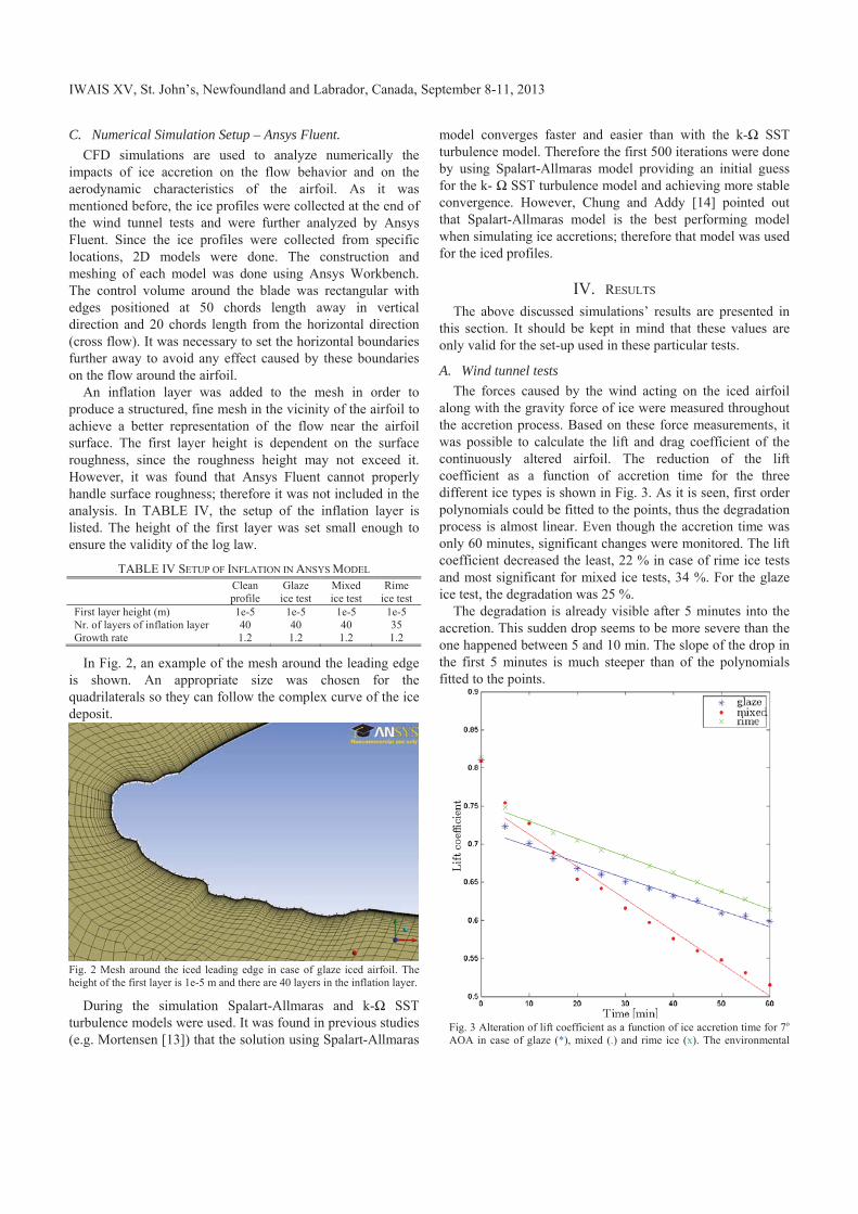
IWAIS XV, St. John’s, Newfoundland and Labrador, Canada, September 8-11, 2013
C. Numerical Simulation Setup – Ansys Fluent. CFD simulations are used to analyze numerically the
impacts of ice accretion on the flow behavior and on the aerodynamic characteristics of the airfoil. As it was mentioned before, the ice profiles were collected at the end of the wind tunnel tests and were further analyzed by Ansys Fluent. Since the ice profiles were collected from specific locations, 2D models were done. The construction and meshing of each model was done using Ansys Workbench. The control volume around the blade was rectangular with edges positioned at 50 chords length away in vertical direction and 20 chords length from the horizontal direction (cross flow). It was necessary to set the horizontal boundaries further away to avoid any effect caused by these boundaries on the flow around the airfoil.
An inflation layer was added to the mesh in order to produce a structured, fine mesh in the vicinity of the airfoil to achieve a better representation of the flow near the airfoil surface. The first layer height is dependent on the surface roughness, since the roughness height may not exceed it. However, it was found that Ansys Fluent cannot properly handle surface roughness; therefore it was not included in the analysis. In TABLE IV, the setup of the inflation layer is listed. The height of the first layer was set small enough to ensure the validity of the log law.
TABLE IV SETUP OF INFLATION IN ANSYS MODEL Clean
profile Glaze ice test
Mixed ice test
Rime ice test
First layer height (m) 1e-5 1e-5 1e-5 1e-5 Nr. of layers of inflation layer 40 40 40 35 Growth rate 1.2 1.2 1.2 1.2
In Fig. 2, an example of the mesh around the leading edge is shown. An appropriate size was chosen for the quadrilaterals so they can follow the complex curve of the ice deposit.
Fig. 2 Mesh around the iced leading edge in case of glaze iced airfoil. The height of the first layer is 1e-5 m and there are 40 layers in the inflation layer.
During the simulation Spalart-Allmaras and k- SST turbulence models were used. It was found in previous studies (e.g. Mortensen [13]) that the solution using Spalart-Allmaras
model converges faster and easier than with the k- SST turbulence model. Therefore the first 500 iterations were done by using Spalart-Allmaras model providing an initial guess for the k- SST turbulence model and achieving more stable convergence. However, Chung and Addy [14] pointed out that Spalart-Allmaras model is the best performing model when simulating ice accretions; therefore that model was used for the iced profiles.
IV. RESULTS The above discussed simulations’ results are presented in
this section. It should be kept in mind that these values are only valid for the set-up used in these particular tests.
A. Wind tunnel tests The forces caused by the wind acting on the iced airfoil
along with the gravity force of ice were measured throughout the accretion process. Based on these force measurements, it was possible to calculate the lift and drag coefficient of the continuously altered airfoil. The reduction of the lift coefficient as a function of accretion time for the three different ice types is shown in Fig. 3. As it is seen, first order polynomials could be fitted to the points, thus the degradation process is almost linear. Even though the accretion time was only 60 minutes, significant changes were monitored. The lift coefficient decreased the least, 22 % in case of rime ice tests and most significant for mixed ice tests, 34 %. For the glaze ice test, the degradation was 25 %.
The degradation is already visible after 5 minutes into the accretion. This sudden drop seems to be more severe than the one happened between 5 and 10 min. The slope of the drop in the first 5 minutes is much steeper than of the polynomials fitted to the points.
Fig. 3 Alteration of lift coefficient as a function of ice accretion time for 7o AOA in case of glaze (*), mixed (.) and rime ice (x). The environmental
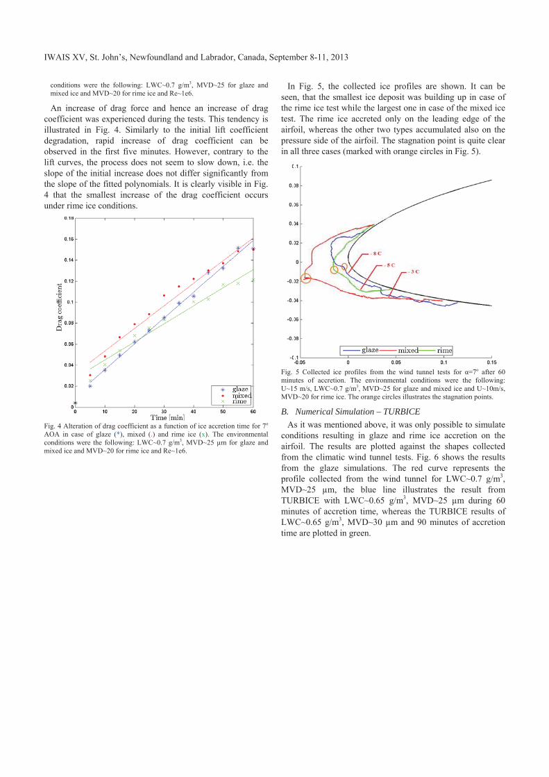
IW
coildeoblislth4 un
FiAcom
WAIS XV, St.
conditions were mixed ice and M
An increase oefficient waslustrated in Fegradation, rbserved in theft curves, the lope of the inihe slope of the
that the smander rime ice
ig. 4 Alteration oAOA in case of gonditions were th
mixed ice and MVD
. John’s, Newf
the following: LMVD~20 for rime
of drag forces experienced Fig. 4. Similarapid increasee first five mprocess does
itial increase de fitted polynoallest increaseconditions.
f drag coefficientglaze (*), mixed he following: LWD~20 for rime ice
foundland and
LWC~0.7 g/m3, ice and Re~1e6.
e and hence aduring the tes
arly to the ine of drag c
minutes. Howes not seem to does not diffeomials. It is cle of the drag
t as a function of (.) and rime ice
WC~0.7 g/m3, MVe and Re~1e6.
d Labrador, Ca
MVD~25 for gl
an increase osts. This tendenitial lift coefcoefficient caver, contrary slow down, i
er significantlylearly visible ig coefficient
f ice accretion tim (x). The enviro
VD~25 μm for gl
anada, Septem
aze and
f drag ency is fficient an be to the
i.e. the y from in Fig. occurs
me for 7o
nmental laze and
Inseenthe testairfopresin a
Fig. minuU~1MVD
B.A
conairfofromfromprofMVTURminLWtime
mber 8-11, 201
n Fig. 5, the n, that the smrime ice test w. The rime ic
foil, whereas tssure side of t
all three cases
5 Collected ice utes of accretion5 m/s, LWC~0.7 D~20 for rime ice
Numerical Sims it was mentiditions resulti
foil. The resulm the climaticm the glaze file collected
VD~25 μm, RBICE with
nutes of accretWC~0.65 g/m3,
e are plotted in
13
collected ice mallest ice depo
while the largece accreted onthe other two the airfoil. The(marked with
profiles from thn. The environm
g/m3, MVD~25 e. The orange circ
mulation – TUioned above, iing in glaze lts are plottedc wind tunnel simulations. from the win
the blue linLWC~0.65 gtion time, wh, MVD~30 μmn green.
profiles are osit was buildest one in casenly on the leatypes accumu
e stagnation porange circles
he wind tunnel temental conditions
for glaze and mixcles illustrates the
URBICE it was only poand rime ice d against the tests. Fig. 6
The red curvnd tunnel for
ne illustrates g/m3, MVD~2hereas the TUm and 90 min
shown. It canding up in case of the mixedading edge ofulated also onpoint is quite cs in Fig. 5).
ests for =7o aftewere the follow
xed ice and U~10 stagnation points
ossible to simuaccretion onshapes colle
shows the resve represents r LWC~0.7 g
the result f25 μm duringRBICE resultnutes of accre
n be se of d ice f the n the clear
er 60 wing: 0m/s, s.
ulate n the
cted sults
the g/m3, from g 60 ts of etion
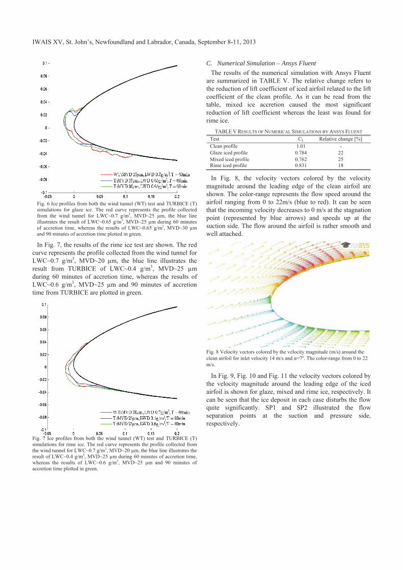
IWAIS XV, St. John’s, Newfoundland and Labrador, Canada, September 8-11, 2013
Fig. 6 Ice profiles from both the wind tunnel (WT) test and TURBICE (T) simulations for glaze ice. The red curve represents the profile collected from the wind tunnel for LWC~0.7 g/m3, MVD~25 μm, the blue line illustrates the result of LWC~0.65 g/m3, MVD~25 μm during 60 minutes of accretion time, whereas the results of LWC~0.65 g/m3, MVD~30 μm and 90 minutes of accretion time plotted in green.
In Fig. 7, the results of the rime ice test are shown. The red curve represents the profile collected from the wind tunnel for LWC~0.7 g/m3, MVD~20 μm, the blue line illustrates the result from TURBICE of LWC~0.4 g/m3, MVD~25 μm during 60 minutes of accretion time, whereas the results of LWC~0.6 g/m3, MVD~25 μm and 90 minutes of accretion time from TURBICE are plotted in green.
Fig. 7 Ice profiles from both the wind tunnel (WT) test and TURBICE (T) simulations for rime ice. The red curve represents the profile collected from the wind tunnel for LWC~0.7 g/m3, MVD~20 μm, the blue line illustrates the result of LWC~0.4 g/m3, MVD~25 μm during 60 minutes of accretion time, whereas the results of LWC~0.6 g/m3, MVD~25 μm and 90 minutes of accretion time plotted in green.
C. Numerical Simulation – Ansys Fluent The results of the numerical simulation with Ansys Fluent
are summarized in TABLE V. The relative change refers to the reduction of lift coefficient of iced airfoil related to the lift coefficient of the clean profile. As it can be read from the table, mixed ice accretion caused the most significant reduction of lift coefficient whereas the least was found for rime ice.
TABLE V RESULTS OF NUMERICAL SIMULATIONS BY ANSYS FLUENT Test CL Relative change [%] Clean profile 1.01 - Glaze iced profile 0.784 22 Mixed iced profile 0.762 25 Rime iced profile 0.831 18
In Fig. 8, the velocity vectors colored by the velocity magnitude around the leading edge of the clean airfoil are shown. The color-range represents the flow speed around the airfoil ranging from 0 to 22m/s (blue to red). It can be seen that the incoming velocity decreases to 0 m/s at the stagnation point (represented by blue arrows) and speeds up at the suction side. The flow around the airfoil is rather smooth and well attached.
Fig. 8 Velocity vectors colored by the velocity magnitude (m/s) around the clean airfoil for inlet velocity 14 m/s and =7o. The color-range from 0 to 22 m/s.
In Fig. 9, Fig. 10 and Fig. 11 the velocity vectors colored by the velocity magnitude around the leading edge of the iced airfoil is shown for glaze, mixed and rime ice, respectively. It can be seen that the ice deposit in each case disturbs the flow quite significantly. SP1 and SP2 illustrated the flow separation points at the suction and pressure side, respectively.
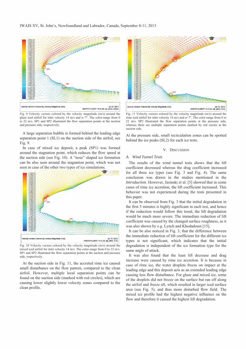
IW
Figltoan
seF
arthcase
FimSPsi
smaifocacl
WAIS XV, St.
ig. 9 Velocity velaze iced airfoil fo 22 m/s. SP1 andnd pressure side, r
A large separeparation poinig. 9. In case of m
round the staghe suction sidean be also seeeen in case of
ig. 10 Velocity vmixed iced airfoil f
P1 and SP2 illustrde, respectively.
At the suctionmall disturbanirfoil. Howevound on the suausing lower lean profile.
. John’s, Newf
ectors colored by for inlet velocity d SP2 illustrated respectively.
ration bubble int 1 (SL1) on
mixed ice depgnation point, e (see Fig. 10en around thethe other two
ectors colored byfor inlet velocity rated the flow sep
n side in Fig. nce on the flover, multiple uction side (mslightly lower
foundland and
the velocity mag14 m/s and =7o.the flow separat
is formed behithe suction sid
posit, a peak which reduce
). A “nose” she stagnation po
types of ice si
y the velocity ma14 m/s. The colorparation points at
11, the accrew pattern, comlocal separat
marked with redr velocity zon
d Labrador, Ca
gnitude (m/s) aro. The color-rangetion points at the
ind the leadingde of the airfo
(SP1) was fes the flow sphaped ice formoint, which wimulations.
gnitude (m/s) aror-range from 0 tot the suction and p
eted rime ice cmpared to thetion points cd circles), whines compared
anada, Septem
ound the e from 0
suction
g edge oil, see
formed peed at mation
was not
ound the 22 m/s. pressure
caused e clean can be ich are to the
Fig. rime22 mwhersucti
At tbeh
A.Th
coeffor conIntrcasebehthis
It the if thwoucoefwas
It the typedegsam
It incrcaseleadcausof ththe areamixflow
mber 8-11, 201
11 Velocity vect iced airfoil for inm/s. SP2 illustrareas there are muion side.
the pressure sind the ice pea
Wind Tunnel he results of fficient decreaall three ice clusion was
roduction. Howes of rime ice avior was nopaper. can be observfirst 5 minutehe reduction wuld be much mfficient was cas also shown bcan be also nimmediate redes is not sigradation is in
me angle of attawas also fo
rease were caue of rime ice,ding edge and sing less flowhe droplets diairfoil and fre
a (see Fig. 5)xed ice profilew and therefor
13
tors colored by thnlet velocity 14 mated the flow se
multiple separation
ide, small recaks (SL2) for
V. DIS
Tests the wind tu
ased whereas types (see Fdrawn in th
wever, Jasinskaccretion, the
ot experienced
ved from Fig. s is highly sigwould follow more severe. Taused by the cby e.g. Lynch anoticed in Fig.duction of lift gnificant, wh
ndependent of ack. ound that theused by rime , the water drthis deposit a
w disturbance. id not freeze oeeze aft, which), and thus me had the higre it caused the
he velocity magnim/s and =7o. Theeparation points n points marked
irculation zoneach ice tests.
CUSSION
unnel tests shthe drag coe
Fig. 3 and Fihe studies mki et al. [5] shoe lift coefficiend during the t
3 that the initgnificant in eac
this trend, thThe immediatechanged surfacand Khodadou. 3, that the dicoefficient fo
hich indicatesthe ice forma
e least lift deice accretion
roplets freeze cts as an extenFor glaze and
on the surface h resulted in l
more disturbedhest negative e highest lift d
itude (m/s) aroune color-range from
at the pressure by red circles a
nes can be spo.
hows that the efficient increaig. 4). The s
mentioned in owed that in snt increased. Ttests presented
tial degradatioch test, and he
he lift degradae reduction ofce roughness, ust [15]. ifference betw
or the differents that the ination type for
ecrease and dn. It is becaus
on impact atnded leading ed mixed ice, so
but ran off alarger iced surd flow field.
influence ondegradation.
nd the m 0 to
side, at the
otted
lift ased ame the
ome This d in
on in ence ation f lift as it
ween t ice
nitial r the
drag se in t the edge ome long rface The
n the
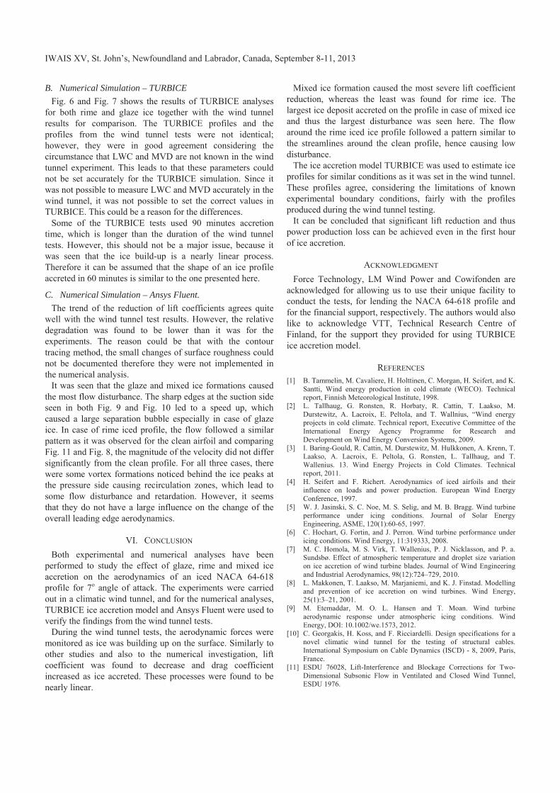
IWAIS XV, St. John’s, Newfoundland and Labrador, Canada, September 8-11, 2013
B. Numerical Simulation – TURBICE Fig. 6 and Fig. 7 shows the results of TURBICE analyses
for both rime and glaze ice together with the wind tunnel results for comparison. The TURBICE profiles and the profiles from the wind tunnel tests were not identical; however, they were in good agreement considering the circumstance that LWC and MVD are not known in the wind tunnel experiment. This leads to that these parameters could not be set accurately for the TURBICE simulation. Since it was not possible to measure LWC and MVD accurately in the wind tunnel, it was not possible to set the correct values in TURBICE. This could be a reason for the differences.
Some of the TURBICE tests used 90 minutes accretion time, which is longer than the duration of the wind tunnel tests. However, this should not be a major issue, because it was seen that the ice build-up is a nearly linear process. Therefore it can be assumed that the shape of an ice profile accreted in 60 minutes is similar to the one presented here.
C. Numerical Simulation – Ansys Fluent. The trend of the reduction of lift coefficients agrees quite
well with the wind tunnel test results. However, the relative degradation was found to be lower than it was for the experiments. The reason could be that with the contour tracing method, the small changes of surface roughness could not be documented therefore they were not implemented in the numerical analysis.
It was seen that the glaze and mixed ice formations caused the most flow disturbance. The sharp edges at the suction side seen in both Fig. 9 and Fig. 10 led to a speed up, which caused a large separation bubble especially in case of glaze ice. In case of rime iced profile, the flow followed a similar pattern as it was observed for the clean airfoil and comparing Fig. 11 and Fig. 8, the magnitude of the velocity did not differ significantly from the clean profile. For all three cases, there were some vortex formations noticed behind the ice peaks at the pressure side causing recirculation zones, which lead to some flow disturbance and retardation. However, it seems that they do not have a large influence on the change of the overall leading edge aerodynamics.
VI. CONCLUSION Both experimental and numerical analyses have been
performed to study the effect of glaze, rime and mixed ice accretion on the aerodynamics of an iced NACA 64-618 profile for 7o angle of attack. The experiments were carried out in a climatic wind tunnel, and for the numerical analyses, TURBICE ice accretion model and Ansys Fluent were used to verify the findings from the wind tunnel tests.
During the wind tunnel tests, the aerodynamic forces were monitored as ice was building up on the surface. Similarly to other studies and also to the numerical investigation, lift coefficient was found to decrease and drag coefficient increased as ice accreted. These processes were found to be nearly linear.
Mixed ice formation caused the most severe lift coefficient reduction, whereas the least was found for rime ice. The largest ice deposit accreted on the profile in case of mixed ice and thus the largest disturbance was seen here. The flow around the rime iced ice profile followed a pattern similar to the streamlines around the clean profile, hence causing low disturbance.
The ice accretion model TURBICE was used to estimate ice profiles for similar conditions as it was set in the wind tunnel. These profiles agree, considering the limitations of known experimental boundary conditions, fairly with the profiles produced during the wind tunnel testing.
It can be concluded that significant lift reduction and thus power production loss can be achieved even in the first hour of ice accretion.
ACKNOWLEDGMENT Force Technology, LM Wind Power and Cowifonden are
acknowledged for allowing us to use their unique facility to conduct the tests, for lending the NACA 64-618 profile and for the financial support, respectively. The authors would also like to acknowledge VTT, Technical Research Centre of Finland, for the support they provided for using TURBICE ice accretion model.
REFERENCES [1] B. Tammelin, M. Cavaliere, H. Holttinen, C. Morgan, H. Seifert, and K.
Santti, Wind energy production in cold climate (WECO). Technical report, Finnish Meteorological Institute, 1998.
[2] L. Tallhaug, G. Ronsten, R. Horbaty, R. Cattin, T. Laakso, M. Durstewitz, A. Lacroix, E. Peltola, and T. Wallnius, “Wind energy projects in cold climate. Technical report, Executive Committee of the International Energy Agency Programme for Research and Development on Wind Energy Conversion Systems, 2009.
[3] I. Baring-Gould, R. Cattin, M. Durstewitz, M. Hulkkonen, A. Krenn, T. Laakso, A. Lacroix, E. Peltola, G. Ronsten, L. Tallhaug, and T. Wallenius. 13. Wind Energy Projects in Cold Climates. Technical report, 2011.
[4] H. Seifert and F. Richert. Aerodynamics of iced airfoils and their influence on loads and power production. European Wind Energy Conference, 1997.
[5] W. J. Jasinski, S. C. Noe, M. S. Selig, and M. B. Bragg. Wind turbine performance under icing conditions. Journal of Solar Energy Engineering, ASME, 120(1):60-65, 1997.
[6] C. Hochart, G. Fortin, and J. Perron. Wind turbine performance under icing conditions. Wind Energy, 11:319333, 2008.
[7] M. C. Homola, M. S. Virk, T. Wallenius, P. J. Nicklasson, and P. a. Sundsbø. Effect of atmospheric temperature and droplet size variation on ice accretion of wind turbine blades. Journal of Wind Engineering and Industrial Aerodynamics, 98(12):724–729, 2010.
[8] L. Makkonen, T. Laakso, M. Marjaniemi, and K. J. Finstad. Modelling and prevention of ice accretion on wind turbines. Wind Energy, 25(1):3–21, 2001.
[9] M. Etemaddar, M. O. L. Hansen and T. Moan. Wind turbine aerodynamic response under atmospheric icing conditions. Wind Energy, DOI: 10.1002/we.1573, 2012.
[10] C. Georgakis, H. Koss, and F. Ricciardelli. Design specifications for a novel climatic wind tunnel for the testing of structural cables. International Symposium on Cable Dynamics (ISCD) - 8, 2009, Paris, France.
[11] ESDU 76028, Lift-Interference and Blockage Corrections for Two-Dimensional Subsonic Flow in Ventilated and Closed Wind Tunnel, ESDU 1976.

IWAIS XV, St. John’s, Newfoundland and Labrador, Canada, September 8-11, 2013
[12] R. J. Schick. Spray technology reference guide: Understanding drop size, bulletin 459c. Technical report, Spraying Systems Co.
[13] K. Mortensen, CFD Simulation of an airfoil with leading edge ice accretion, Department of Mechanical Engineering, Technical University of Denmark, 2008
[14] J.J. Chung and H.E. Addy, Jr. A Numerical Evaluation of Icing effects on a Natural Laminar Flow Airfoil. NASA TM-2000-209775, January 2000.
[15] F. T. Lynch and A. Khodadoust. Effects of ice accretions on aircraft aerodynamics. Progress in Aerospace Sciences, 37(8):669-767, 2001.
References
E. Aakervik. Nanortalik, Nanortalik municipality, Greenland - Analysis of Wind Mea-surements. Technical report, Kjeller Vindteknikk, KVT/EAA/2011/R075, 2011.
I. Abbott and A. von Doenhoff. Theory of Wing Sections. Including a Summary of AirfoilData. Courier Dover Publications, 1959.
H. E. Addy. Ice Accretions and Icing Effects for Modern Airfoils. Technical Report April,NASA’s Glenn Research Center, Cleveland, Ohio, 2000.
H. E. Addy, A. P. Broeren, J. G. Zoeckler, and S. Lee. A Wind Tunnel Study of IcingEffects on a Business Jet Airfoil. In American Institute of Aeronautics and Astronautics,Aerospace Sciences Meeting and Exhibit, number February, 2003. ISBN 2003212124.
Advisory Circular. Effect of Icing on Aircraft Control and Airplane Deice and Anti-iceSystems. 1996.
AMTI. MC5 Force and Torque Transducer, 2000. URL http://www.summitmedsci.co
.uk/documents/MC5.pdf.
C. Arbez, A. Amosse, and M. Wadham-Gagnon. Met Mast Configuration Guidelinesin Cold Climate. In IWAIS XV, St. John’s, Newfoundland and Labrador, Canada,September, 2013.
I. Baring-Gould, R. Cattin, M. Durstewitz, M. Hulkkonen, A. Krenn, T. Laakso,A. Lacroix, E. Peltola, G. Ronsten, L. Tallhaug, and T. Wallenius. 13. Wind EnergyProjects in Cold Climates. Technical report, 2011.
L. Battisti. Relevance of Icing. Technical report, DTU Wind turbine ice preventionsystems selection and design (41326 ) lecture notes, Technical University of Denmark,2008.
L. Battisti. Relevance of icing. Technical report, DTU Wind turbine ice preventionsystems selection and design (41326 ) lecture notes, 2009.
L. Battisti, R. Fedrizzi, and A. Brighenti. Sea Ice and Icing Risk for Offshore WindTurbines. In Owemes 2006, 20-22 April. Citavecchia, Italy, pages 20–22, 2006.
L. Blumenthal, G. Busch, A. Broeren, and M. Bragg. Issues in Ice Accretion AerodynamicSimulation on a Subscale Model. 44th AIAA Aerospace Sciences Meeting and Exhibit,pages 1–20, Jan. 2006.
N. Bose. Icing on a Small Horizontal-Axis Wind Turbine - Part 1 : Glaze Ice Profiles.Journal of Wind Engineering and Industrial Aerodynamics, 45, 1992.
REFERENCES
M. Bragg, A. Broeren, and L. Blumenthal. Iced-Airfoil Aerodynamics. Progress inAerospace Sciences, 41(5):323–362, July 2005. ISSN 03760421.
M. B. Bragg, A. P. Broeren, H. E. Addy, and M. G. Potapczuk. Airfoil Ice-Accretion Aero-dynamics Simulation. Collection of Technical Papers - 45th AIAA Aerospace SciencesMeeting, (January), 2007.
S. A. Brandt. Chapter 4: Wings and Airplanes. In Introduction to Aeronautics: A DesignPerspective, page 509. American Institute of Aeronautics and Astronautics, 2004.
V. Carlsson. Measuring Routines of Ice Accretion for Wind Turbine Applications. MasterThesis, Umeaa Univesitet, 2009.
F. M. Catalano and P. R. Caixeta Jr. Wind Tunnel Wall Boundary Layer Control for 2DHigh Lift Wing Testing. In 24th International Congress of the Aeronautical SCIENCES,2004.
R. Cattin. Icing of Wind Turbines. Elforsk report 12:13. Technical Report January, 2012.
J. J. Chung and H. E. J. Addy. A Numerical Evaluation of Icing Effects on a NaturalLaminar Flow Airfoil. In 38th Aerospace Sciences Meeting & Exhibit, January 10-13,2000.
T. Dahl. Summit Station Wind Power Pilot Project. Technical report, CH2M Hill PolarServices, 2009.
ESDU 76028. Lift-Interference and Blockage Corrections for Two-Dimensional SubsonicFlow in Ventilated and Closed Wind Tunnel. Technical report, 1976.
M. Etemaddar, M. O. L. Hansen, and T. Moan. Wind Turbine Aerodynamic ResponseUnder Atmospheric Icing Conditions. Wind Energy, 2012.
S. Fikke, G. Ronsten, A. Heimo, S. Kunz, M. Ostrozlik, J. Sabata, B. Wareing,B. Wichura, J. Chum, T. Laakso, and L. Makkonen. COST 727 : Atmospheric Icingon Structures Measurements and data collection on icing : State of the Art. TechnicalReport 75, Publication of MeteoSwiss, 2006.
G. Fortin and J. Perron. Spinning Rotor Blade Tests in Icing Wind Tunnel. In AIAA2009-4260, 1st AIAA Atmospheric and Space Environments Conference, San Antonio,TX, number June, pages 1–16, 2009.
G. Fortin, J.-L. Laforte, and A. Beisswenger. Prediction of Ice Shapes on NACA0012 2DAirfoil. SAE Technical Papers 2003-01-2154., June 2003.
G. Fortin, P. J. Perron, and P. A. Ilinca. Behaviour and Modeling of Cup Anemome-ters under Icing Conditions. In XI. International Workshop on Atmospheric Icing onStructures, Montreal, Canada, number June, 2005.
R. W. Fox, A. T. McDonald, and P. J. Pritchard. Introduction to Fluid Mechanics. JohnWiley & Sons Inc., 2009.
REFERENCES
R. W. Gent, N. P. Dart, and J. T. Cansdale. Aircraft Icing. Philosophical Transactionsof the Royal Society A: Mathematical, Physical and Engineering Sciences, 358(1776):2873–2911, Nov. 2000. ISSN 1364-503X.
C. T. Georgakis, H. Koss, and F. Ricciardelli. Design Specifications for a Novel ClimaticWind Tunnel for the Testing of Structural Cables. In International Symposium onCable Dynamics (ISCD), Paris, France, number 1, 2009.
Germanischer Lloyd Wind Energy GmbH. GL Wind Technical Note 067 Certification ofWind Turbines for Extreme Temperatures , Scope of Assessment, Revision 3. Technicalreport, 2009.
W. G. Habashi, F. Morency, and H. Beaugendre. FENSAP-ICE : a comprehensive 3DSimulation Tool for In-flight Icing. In 7th International Congress of Fluid Dynamics andPropulsion, Sharm-El-Sheikh, Egypt, December, number December, pages 1–7, 2001.
C. Hochart, G. Fortin, and J. Perron. Wind Turbine Performance Under Icing Conditions.Wind Energy, 11:319–333, 2008.
HoloOptics. User Guide. T 40 series of Icing Rate Sensors. Technical report. URLhttp://holooptics.net/.
M. C. Homola, P. J. Nicklasson, and P. a. Sundsbø. Ice Sensors for Wind Turbines. ColdRegions Science and Technology, 46(2):125–131, Nov. 2006. ISSN 0165232X.
M. C. Homola, T. Wallenius, L. Makkonen, and P. J. Nicklasson. The relationship betweenchord length and rime icing on wind turbines. Wind Energy, 13(7):627–632, 2009.
M. C. Homola, M. S. Virk, T. Wallenius, P. J. Nicklasson, and P. a. Sundsbø. Effectof Atmospheric Temperature and Droplet Size Variation on Ice Accretion of WindTurbine Blades. Journal of Wind Engineering and Industrial Aerodynamics, 98(12):724–729, Dec. 2010a. ISSN 01676105.
M. C. Homola, T. Wallenius, L. Makkonen, P. J. Nicklasson, and P. A. Sundsbø. TurbineSize and Temperature Dependence of Icing on Wind Turbine Blades. Wind Engineering,34(6):615–628, 2010b.
IEA-RETD. Renewable Energies for Remore Areas and Islands (REMOTE). Technicalreport, IEA Renewable Energy Technology Deployment, 2012.
A. Ilinca. Analysis and Mitigation of Icing Effects on Wind Turbines. In I. Al-Bahadly,editor, Wind Turbines, chapter 8., pages 177–214. InTech, 2011.
ISO 12494. Atmospheric icing of Structures. Technical report, ISO Copyright Office,Geneva, Switzerland, 2001.
W. J. Jasinski, S. C. Noe, M. S. Selig, and M. B. Bragg. Wind Turbine Performance UnderIcing Conditions. Transactions of the ASME. Journal of Solar Energy Engineering, 120(1):60–65, 1997.
REFERENCES
L. E. Kollar, M. Farzaneh, and A. R. Karev. Modeling Droplet Collision and Coales-cence in an Icing Wind Tunnel and the Influence of These Processes on Droplet SizeDistribution. International Journal of Multiphase Flow, 31(1):69–92, Jan. 2005. ISSN03019322.
H. Koss and M. S. M. Lund. Experimental Investigation of Aerodynamic Instability of IcedBridge Cable Sections. In 6th European and African Conference on Wind Engineering,Cambridge, UK, 2013.
A. G. Kraj and E. L. Bibeau. Icing Characteristics and Mitigation Strategies for WindTurbines in Cold Climates. 2006.
T. Laakso, M. Durstewitz, R. Horbaty, A. Lacroix, E. Peltola, G. Ronsten, L. Tallhaug,and T. Wallenius. State-of-the-art of Wind Energy in Cold Climates. Technical report,IEA Task 19 - Wind Energy in Cold Climates, 2009.
F. T. Lynch and A. Khodadoust. Effects of Ice Accretions on Aircraft Aerodynamics.Progress in Aerospace Sciences, 37(2001):669–767, 2001.
L. Makkonen. Atmospheric Icing on Sea Structures. U.S. Army Cold Regions Researchand Engineering Laboratory, Hanover, New Hampshire, 1984.
L. Makkonen. Models for the Growth of Rime, Glaze, Icicles and Wet Snow on Struc-tures. Philosophical Transactions of the Royal Society A: Mathematical, Physical andEngineering Sciences, 358(1776):2913–2939, Nov. 2000. ISSN 1364-503X.
L. Makkonen, T. Laakso, M. Marjaniemi, and K. J. Finstad. Modeling and prevention ofice accretion on wind turbines. Wind Energy, 25(1):3–21, 2001.
K. Mortensen. CFD Simulation of an Airfoil with Leading Edge Ice Accretion. Masterthesis. Department of Mechanical Engineering, Technical University of Denmark, 2008.
Navigant Research. BTM Wind Report: World Market Update 2012. International WindEnergy Development Forecast 2013-2017. 2012.
O. Parent and A. Ilinca. Anti-icing and De-icing Techniques for Wind Turbines : CriticalReview. Cold Regions Science and Technology, pages 1–9, 2010. ISSN 0165-232X.
T. Reid, G. Baruzzi, and I. Ozcer. FENSAP - ICE Simulation of Icing on Wind TurbineBlades , Part 1 : Performance Degradation. In 51st AIAA Aerospace Sciences Meetingincluding the New Horizons Forum and Aerospace Exposition 07 - 10 January 2013,Grapevine (Dallas/Ft. Worth Region), Texas, number January, 2013.
E. Sagol, M. Reggio, and A. Ilinca. Issues Concerning Roughness on Wind Turbine Blades.Renewable and Sustainable Energy Reviews, 23:514–525, July 2013. ISSN 13640321.
R. J. Schick. Spray technology reference guide: Understanding drop size, bulletin 459c.Technical report, Spraying Systems Co., 2008.
H. Seifert and F. Richert. Aerodynamics of iced Airfoils and Their Influence on Loadsand Power Production. In European Wind Energy Conference, Dublin Castle, Ireland,number October, pages 458–463, 1997.
REFERENCES
H. Seifert and F. Richert. A Recipe to Estimate Aerodynamics and Loads on Iced RotorBlades. In Paper presented at BOREAS IV, Enontekio, Hetta, Finland, number March1998, pages 1–11, 1998.
J. Shin, B. Berkowitz, H. Chen, and T. Cebeci. Prediction of Ice Shapes and Their Effecton Airfoil Performance. In 29th Aerospace Sciences Meeting. AIAA-91-0264, 1991.
B. Tammelin, M. Cavaliere, H. Holttinen, C. Morgan, and H. Seifert. Wind EnergyProduction in Cold Climate. Technical Report January 1996, 1998.
B. Tammelin, H. Dobesch, M. Durstewich, H. Ganander, G. Kury, T. Laakso, and E. Pel-tola. Wind Turbines in Icing Environment : Improvement of Tools for Siting , Cer-tification and Operation - NEW ICETOOLS. Finnish Meteorological Institute, 2005.ISBN 9516976182.
O. Ulleberg and A. Moerkved. Renewable Energy and Hydrogen System Concepts forRemote communities in the West Nordic Region - The Nolsoy Case Study. Technicalreport, 2008.
F. Villalpando, M. Reggio, and A. Ilinca. Numerical Study of Flow Around Iced WindTurbine Airfoil. Engineering Applications of Computational Fluid Mechnanics, 6(1):39–45, 2012.
A. Villumsen, K. Jakobsen, M. Holtergaard Nielsen, J. Dragsted, E. Larsen, andK. Schaldemose Hansen. Fyrtaarnsprojekt III - afsluttende rapport 2009. Technical re-port, Arctic Technology Center, Deparment of Civil Engineering, Technical Universityof Denmark, 2009.
M. S. Virk, M. C. Homola, and P. J. Nicklasson. Effect of Rime Ice Accretion on Aero-dynamic Characteristics of Wind Turbine Blade Profiles. Wind Engineering, 34(2):207–218, Mar. 2010a. ISSN 0309-524X.
M. S. Virk, M. C. Homola, and P. J. Nicklasson. Relation Between Angle of Attack andAtmospheric Ice Accretion on Large Wind Turbine’ s Blade. Wind Engineering, 34(6):607–614, 2010b.
M. S. Virk, M. C. Homola, and P. J. Nicklasson. Atmospheric Icing on Large WindTurbine Blades. International Journal of Energy and Environment, 3(1):1–8, 2012.
W. B. Wright, M. G. Potapczuk, and L. H. Levinson. Comparison of LEWICE andGlennICE in the SLD Regime. In 46th Aerospace Sciences Meeting and Exhibit, Reno,Nevada, number September, 2008.

DTU Vindenergi er et institut under Danmarks Tekniske Universitet med en unik integration af forskning, uddannelse, innovation ogoffentlige/private konsulentopgaver inden for vindenergi. Vores aktiviteter bidrager til nye muligheder og teknologier inden for udnyttelse af vindenergi, både globalt og nationalt. Forskningen har fokus på specifikke tekniske og videnskabelige områder, der er centrale for udvikling, innovation og brug af vindenergi, og som danner grundlaget for højt kvalificerede uddannelser på universitetet.
Vi har mere end 240 ansatte og heraf er ca. 60 ph.d. studerende. Forskningen tager udgangspunkt i ni forskningsprogrammer, der er organiseret i tre hovedgrupper: vindenergisystemer, vindmølleteknologi og grundlagsskabende forskning.
Danmarks Tekniske Universitet Institut for Vindenergi Nils Koppels Allé Bygning 403 2800 Kgs. Lyngby Phone 46 77 50 85
[email protected] www.vindenergi.dtu.dk