Embed Size (px)
Citation preview

ICES REPORT 14-03
February 2014
Isogeometric Boundary-Element Analysis for theWave-Resistance Problem using T-splines
by
A.I. Ginnis, K.V. Kostas, C.G. Politis, P.D. Kaklis, K.A. Belibassakis, Th.P. Gerostathis, M.A. Scott,
T.J.R Hughes
The Institute for Computational Engineering and SciencesThe University of Texas at AustinAustin, Texas 78712
Reference: A.I. Ginnis, K.V. Kostas, C.G. Politis, P.D. Kaklis, K.A. Belibassakis, Th.P. Gerostathis, M.A. Scott,T.J.R Hughes, "Isogeometric Boundary-Element Analysis for the Wave-Resistance Problem using T-splines,"ICES REPORT 14-03, The Institute for Computational Engineering and Sciences, The University of Texas atAustin, February 2014.

Isogeometric Boundary-Element Analysis for the Wave-ResistanceProblem using T-splines
A.I. Ginnisa,∗, K.V. Kostasb, C.G. Politisb, P.D. Kaklisa,c, K.A. Belibassakisa,Th.P. Gerostathisb, M.A. Scottd, T.J.R Hughese
aSchool of Naval Architecture & Marine Engineering, National Technical University of AthensbDepartment of Naval Architecture, Technological Educational Institute of Athens
cDepartment of Naval Architecture, Ocean and Marine Engineering, University of StrathclydedDepartment of Civil and Environmental Engineering, Brigham Young University
eInstitute for Computational Engineering and Sciences, The University of Texas at Austin
Abstract
In this paper we couple collocated Boundary Element Methods (BEM) with unstructured analysis-
suitable T-spline surfaces for solving a linear Boundary Integral Equation (BIE) arising in the
context of a ship-hydrodynamic problem, namely the so-called Neumann-Kelvin problem, following
the formulation by Brard (1972) [1] and Baar & Price (1988) [2]. The local-refinement capabilities
of the adopted T-spline bases, which are used for representing both the geometry of the hull and
approximating the solution of the associated BIE, in accordance with the Isogeometric concept
proposed by Hughes et al. (2005) [3], lead to a solver that achieves the same error level for many
fewer degrees of freedom as compared with the corresponding NURBS-based Isogeometric-BEM
solver recently developed in Belibassakis et al. (2013) [4]. In this connection, this paper makes a
step towards integrating modern CAD representations for ship-hulls with hydrodynamic solvers of
improved accuracy and efficiency, which is a prerequisite for building efficient ship-hull optimizers.
1. Introduction
Wave-making resistance is a very important component, which may contribute up to 50% - or
even more - to the total resistance of a ship, especially for relatively “full” hull forms and/or at
high speeds. Experience has shown that the wave-making resistance component is quite sensitive
to changes to hull-form shape and significant reduction can be achieved without affecting cargo
capacity. During the last 50 years, the interest in numerical methods for calculating ship wave
resistance has been constantly growing. Computations are performed using a variety of techniques,
ranging from the simple Michell’s thin-ship theory [5] to extremely complex and costly methods
such as the fully non-linear Reynolds Averaged Navier Stokes Equations (RANSE) [6, 7, 8]; see
the reports by the International Towing Tank Conference ([9, 10, 11]) and the references cited
therein.
∗Corresponding author: [email protected]
Preprint submitted to Elsevier February 10, 2014

In all proposed methods a CAD model of the ship hull is required. However, analysis-suitable
models cannot be, in general, automatically derived from CAD models. Data exchange between
CAD and analysis methods requires many time-consuming, preparatory steps. For example, the
popular meshing approach is generally time consuming and provides only an approximation of
the exact CAD geometry. Furthermore, a recalculation of the generated mesh is required for
even slight changes in the exact geometry. Thus, the lack of geometric exactness along with the,
generally, cumbersome mesh regeneration render the requirements for rapid convergence and/or
high precision prohibitive. These deficiencies in the current engineering analysis approach also
preclude successful application of other procedures such as design optimization. In this case, the
CAD-geometry-to-mesh mapping needs to be automatic and tightly integrated with the analysis
solver and the optimizing environment. Enabling the automatic generation of geometrically exact
and analysis suitable models could pave the way towards overcoming the aforementioned barriers.
This aim can be achieved by appealing to IsoGeometric Analysis (IGA), introduced by Hughes
et al. [12, 3] and Cottrell et al. [13, 14], which provides a direct and tight link between CAD
and Computer Aided Engineering (CAE). This link is achieved by using the very same basis for
representing both the geometry and the physical quantities employed in the analysis.
A number of candidate geometry representations can be used in the context of IGA. The
geometrical representation, that is so far prevailing in CAD industry, is NURBS (Non-Uniform
Rational B-Splines) [15]. NURBS representations offer: 1) convenience in modeling free-form
parametric surfaces, 2) exact representation of all quadratic curves and surfaces that frequently
occur in Mechanical-Engineering Design and 3) availability of many efficient and numerically-stable
algorithms for their evaluation. NURBS also possess some mathematical properties that are useful
from the analysis point of view: a) refinability, such as the conventional h- (knot insertion) and
p- (degree elevation) refinement schemes, as well as a more flexible refinement pattern, the so-
called k-refinement, which is suitable for higher-order approximations, and b) high smoothness,
i.e., Cp−1-continuity for NURBS of degree p ≥ 2, which prohibits derivative-jumps, thus, yielding
more accurate results.
Isogeometric Analysis has been so far mainly applied in the FEM context, [13, 3], where
the basic preprocessing step is to develop good quality two- and three-dimensional (trivariate)
representations of the computational domain. The latter is far from being a trivial problem and
although different methods have been developed, e.g., lofting, swept-volume parameterization,
Coons patches, etc., the literature is still lacking of a general and mature methodology. On the
other hand, this approach differs from that adopted in contemporary CAD systems, namely the
so-called Boundary representation (B-rep) of solids. In order to overcome these difficulties, a new
approach for exploiting Isogeometric analysis has been presented. It is based on the boundary
integral formulation of the problem considered, where the governing equations and the boundary
2

conditions of the problem are transformed into a boundary integral equation (weakly singular
or singular) on the boundary (or a portion of the boundary) using the Green’s function of the
problem to be treated [16, 17, 4, 18, 19, 20, 21]. This approach is widely used in free-surface
hydrodynamics, and especially in exterior potential-flow problems, due to the infinite extent of
the fluid domain.
In the above context, our previous work [4], has demonstrated the applicability and advantages
of the Isogeometric approach to free-surface problems and especially to a linearized version of the
wave-resistance problem, the so called “Neumann-Kelvin wave-resistance” problem, as initially
proposed by Brard (1972) [1]. In this version of the problem, the potential flow theory is adopted
and the non-linear effects stemming from the presence of the unknown free surface are neglected,
while the three-dimensional character of the problem is retained. For the numerical solution of
the resulting linear problem a Boundary-Element Method (BEM) was formulated, implemented
by means of a Kelvin-wave source distribution over the wetted part of the hull and its intersection
with the undisturbed free surface [2]. A multi-patch tensor product NURBS surface was used for
the representation of the wetted ship hull boundary and the very same NURBS basis was used
for the approximation of the unknown source density. The Isogeometric scheme was implemented
by collocating at the images of the Greville abscissae of the associated knot vectors and knot
insertion (h-refinement) is used as our refinement strategy. The enhanced accuracy and efficiency
of the proposed NURBS based IsoGeometric Analysis BEM (IGA-BEM) has been demonstrated
by comparing the numerical results obtained for a variety of geometrical configurations against
analytical solutions and/or experimental data (where available) as well as predictions provided by
low-order panel methods and higher-order BEMs. The tested configurations included a prolate
spheroid in an infinite domain, a three-axial ellipsoid in a semi-infinite domain, a submerged
prolate spheroid under the free surface and three free-surface piercing hulls, namely the standard
Wigley hull, a Series 60 and the so-called KRISO container ship hull [22].
However, the use of NURBS in Isogeometric Analysis exhibits some deficiencies:
1. Multi-patch representations suffer from gaps and overlaps at patch boundaries.
2. Due to their tensor-product nature a large number of NURBS control points is not unlikely
to be superfluous, in the sense that they contain no significant geometric information. As
a consequence, the resulting basis for approximating the physical quantities of interest, is
“overloaded” with redundant detail in areas where these quantities are expected to exhibit
low variation.
3. Refinement requires the insertion of entire rows/columns of control points, thus increasing
complexity and implementation effort.
3

4. The limitations of rectangular topology lead to multi-patch representations when complex ob-
jects, as e.g., ship hulls, are under consideration. This limitation has an additional side-effect
as multi-patch configurations can only secure a C0 basis continuity across patch boundaries,
canceling, in this way, the intrinsic higher smoothness of a single NURBS patch.
T-splines [23, 24] constitute a recently developed generalization of NURBS technology that
removes most of the above mentioned NURBS deficiencies. It is worth noticing that in the
computer-aided ship-design literature one can already cite works arguing that NURBS do not
offer the proper frame for ship design [25] and aspire to alternative representations, which include
T-splines [26]. The main advantages of T-splines technology are:
1. T-splines permit representation of complex objects with a single T-spline patch.
2. A T-spline control grid is allowed to have partial rows of control points, terminating in
T-junctions, which allows for local refinement.
3. T-junctions permit the significant reduction of superfluous control points.
4. It is possible to merge multiple NURBS patches into a single, gap-free T-spline.
Our aim in the present work is to make a first step towards exploiting the advantages of T-
splines technology in Isogeometric analysis (TS-IGA) for ship hydrodynamic analysis. The higher
smoothness of a single T-spline surface along with the ability for local refinement allow us to
achieve enhanced convergence rates with considerably fewer degrees of freedom when compared to
our prior NURBS approach. This will permit our T-spline based IGA-BEM solver to be embedded
with significantly lower cost in any optimization process for designing ship hulls with minimum
wave resistance.
The remaining part of this paper is structured in 4 sections. Section 2 presents the formulation
of the problem while section 3 provides a brief overview of T-splines. We then proceed with
the formulation of the problem in the Isogeometric T-spline BEM (TS-IGA-BEM) context and we
conclude our work with two numerical examples demonstrating the achieved enhanced convergence:
a prolate spheroid in infinite domain and a surface piercing ship hull.
2. Formulation of the problem
Let Oxyz be a right-handed rectangular coordinate system with the z−axis directed vertically
upwards; see Figure 1. We consider the flow of a uniform stream with velocity U = (−U, 0, 0) of
an ideal fluid with a free surface incident upon a surface piercing or fully submerged body D.
It is convenient to decompose the velocity potential Φ in the form:
Φ = −Ux+ ϕ, (1)
4

Figure 1: Geometric configuration of the Neumann-Kelvin problem for a surface piercing body.
where ϕ is the disturbance potential due to the presence of the submerged body. The disturbance
potential must satisfy the Laplace equation (see, e.g., [2]):
4ϕ = 0 in D+, (2)
where D+ denotes the unbounded fluid domain outside the body D limited above by the plane
z = 0. The body boundary condition is
∂ϕ
∂n= −U · n on S, (3)
where n = (nx, ny, nz) is the unit normal directed inwards with respect to the domain D+ and
S = ∂D is the boundary of the body D. The free-surface conditions satisfied on the unknown free
surface z = η(x, y) are:
(i) The kinematic condition, stating that on the free surface the flow velocity must be tangential:
(−U + ϕx)ηx + ϕyηy − ϕz = 0. (4)
(ii) The dynamic condition, stating that the pressure on the free surface must be constant:
gη − Uϕx +1
2(ϕx
2 + ϕy2 + ϕz
2) = 0, (5)
with g denoting the gravitational acceleration. In the theory of infinitesimal waves the above
conditions on the free surface are linearized by neglecting products and squares of “small” quan-
tities (stemming from the fact that the disturbance velocities are considered to be of higher order
with respect to U) and by applying the resulting equations on the undisturbed free surface z = 0
5
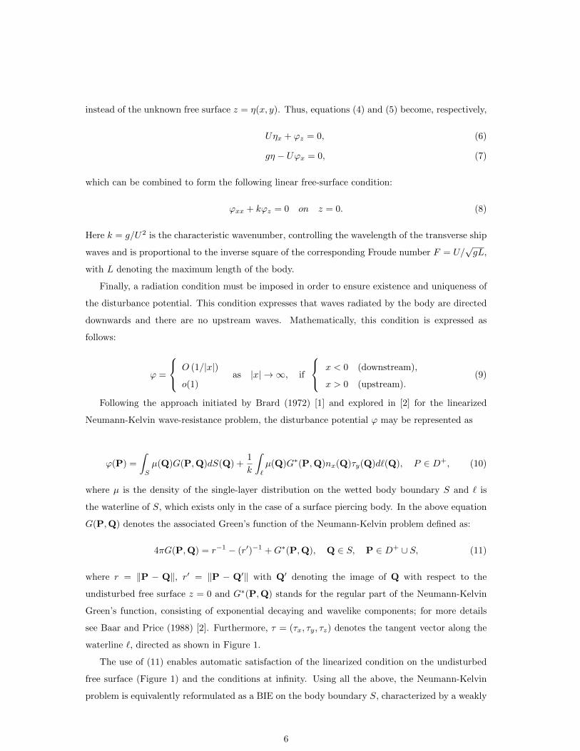
instead of the unknown free surface z = η(x, y). Thus, equations (4) and (5) become, respectively,
Uηx + ϕz = 0, (6)
gη − Uϕx = 0, (7)
which can be combined to form the following linear free-surface condition:
ϕxx + kϕz = 0 on z = 0. (8)
Here k = g/U2 is the characteristic wavenumber, controlling the wavelength of the transverse ship
waves and is proportional to the inverse square of the corresponding Froude number F = U/√gL,
with L denoting the maximum length of the body.
Finally, a radiation condition must be imposed in order to ensure existence and uniqueness of
the disturbance potential. This condition expresses that waves radiated by the body are directed
downwards and there are no upstream waves. Mathematically, this condition is expressed as
follows:
ϕ =
O (1/|x|)o(1)
as |x| → ∞, if
x < 0 (downstream),
x > 0 (upstream).(9)
Following the approach initiated by Brard (1972) [1] and explored in [2] for the linearized
Neumann-Kelvin wave-resistance problem, the disturbance potential ϕ may be represented as
ϕ(P) =
ˆS
µ(Q)G(P,Q)dS(Q) +1
k
ˆ`
µ(Q)G∗(P,Q)nx(Q)τy(Q)d`(Q), P ∈ D+, (10)
where µ is the density of the single-layer distribution on the wetted body boundary S and ` is
the waterline of S, which exists only in the case of a surface piercing body. In the above equation
G(P,Q) denotes the associated Green’s function of the Neumann-Kelvin problem defined as:
4πG(P,Q) = r−1 − (r′)−1 +G∗(P,Q), Q ∈ S, P ∈ D+ ∪ S, (11)
where r = ‖P − Q‖, r′ = ‖P − Q′‖ with Q′ denoting the image of Q with respect to the
undisturbed free surface z = 0 and G∗(P,Q) stands for the regular part of the Neumann-Kelvin
Green’s function, consisting of exponential decaying and wavelike components; for more details
see Baar and Price (1988) [2]. Furthermore, τ = (τx, τy, τz) denotes the tangent vector along the
waterline `, directed as shown in Figure 1.
The use of (11) enables automatic satisfaction of the linearized condition on the undisturbed
free surface (Figure 1) and the conditions at infinity. Using all the above, the Neumann-Kelvin
problem is equivalently reformulated as a BIE on the body boundary S, characterized by a weakly
6

singular kernel,
µ(P)
2−ˆS
µ(Q)∂G(P,Q)
∂n(P)dS(Q)− 1
k
ˆ`
µ(Q)∂G∗(P,Q)
∂n(P)nx(Q)τy(Q)d`(Q) = U · n(P),
P,Q ∈ S. (12)
From the solution of the above integral equation, various quantities, such as velocity, pressure
distribution and ship wave pattern can be obtained. Specifically, total flow velocity and pressure
are readily obtained by
w = U +∇ϕ, (13)
p = p∞ +ρ
2(U2 − ‖w‖2)− ρgz, (14)
where ρ is the fluid density and p∞ is the ambient pressure. The deviation of pressure p from p∞
is measured via the non-dimensional pressure coefficient
Cp =p− p∞ρ2U
2= 1− ‖w‖
2 + 2gz
U2. (15)
Finally, the free-surface elevation is obtained by
η(x, y) = (U/g) · ϕx(x, y; z = 0). (16)
We conclude this section by noting that in the case of a fully submerged body the above
formulation should be modified by dropping the waterline integral in Eqs. (10) and (12).
3. T-splines: A brief introduction
In this section, we present a brief overview of T-spline technology. For additional details the
interested reader is referred to Sederberg et al. (2003a,b) [23, 27], Sederberg et al. (2004) [28],
Bazilevs et al. (2010) [24], Scott et al. (2011) [29] and Scott et al. (2012) [30]. In what follows
we focus on cubic T-spline surfaces due to their predominance in industry. We denote the spatial
and parametric dimensions by ds and dp, respectively. We denote an element index by e and the
number of non-zero basis functions over an element e by n.
3.1. The unstructured T-mesh
An important object of interest underlying T-spline technology is the T-mesh. For surfaces,
a T-mesh is a polygonal mesh and we will refer to the constituent polygons as elements or,
equivalently, faces. Each element is a quadrilateral whose edges are permitted to contain T-
junctions – vertices that are analogous to hanging nodes in finite elements. A control point,
PA ∈ Rds , ds = 2, 3 and a control weight, wA ∈ R, where the index A denotes a global control
point number, is assigned to every vertex in the T-mesh. The valence of a vertex is the number of
7

Figure 2: An unstructured T-mesh. Extraordinary points are denoted by hollow circles and T-junctions are denotedby hollow squares.
edges that touch the vertex. An extraordinary point is an interior vertex that is not a T-junction
and whose valence does not equal four.
Figure 2 shows an unstructured T-mesh. Notice the valence three and valence five at extraor-
dinary points denoted by hollow circles. The single T-junction is denoted by a hollow square.
To define a basis, a valid knot interval configuration must be assigned to the T-mesh. A knot
interval is a non-negative real number assigned to an edge. A valid knot interval configuration
requires that the knot intervals on opposite sides of every element sum to the same value. In
this paper, we require that the knot intervals for spoke edges of an individual extraordinary point
either be all non-zero or all zero.
3.2. Bezier extraction
In this paper, we develop T-splines from the finite element point-of-view, utilizing Bezier
extraction [31, 29]. The idea is to extract the linear operator which maps the Bernstein polynomial
basis on Bezier elements to the global T-spline basis. The linear transformation is defined by a
matrix referred to as the extraction operator and denoted by Ce. The transpose of the extraction
operator maps the control points of the global T-spline to the control points of the Bernstein
polynomials. Figure 3 illustrates the idea for a B-spline curve. This provides a finite element
representation of T-splines, and facilitates the incorporation of T-splines into existing finite element
programs. Only the shape function subroutine needs to be modified. All other aspects of the
finite element program remain the same. Additionally, Bezier extraction is automatic and can be
applied to any T-spline regardless of topological complexity or polynomial degree. In particular,
it represents an elegant treatment of T-junctions, referred to as hanging nodes in finite element
analysis.
8
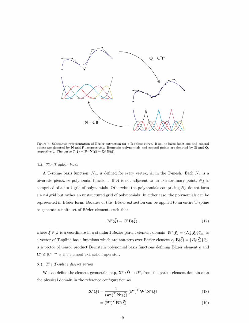
Q = CTP
N = CB
Figure 3: Schematic representation of Bezier extraction for a B-spline curve. B-spline basis functions and controlpoints are denoted by N and P, respectively. Bernstein polynomials and control points are denoted by B and Q,respectively. The curve T (ξ) = PTN(ξ) = QTB(ξ).
3.3. The T-spline basis
A T-spline basis function, NA, is defined for every vertex, A, in the T-mesh. Each NA is a
bivariate piecewise polynomial function. If A is not adjacent to an extraordinary point, NA is
comprised of a 4× 4 grid of polynomials. Otherwise, the polynomials comprising NA do not form
a 4×4 grid but rather an unstructured grid of polynomials. In either case, the polynomials can be
represented in Bezier form. Because of this, Bezier extraction can be applied to an entire T-spline
to generate a finite set of Bezier elements such that
Ne(ξ) = CeB(ξ), (17)
where ξ ∈ Ω is a coordinate in a standard Bezier parent element domain, Ne(ξ) = Nea(ξ)na=1 is
a vector of T-spline basis functions which are non-zero over Bezier element e, B(ξ) = Bi(ξ)mi=1
is a vector of tensor product Bernstein polynomial basis functions defining Bezier element e and
Ce ∈ Rn×m is the element extraction operator.
3.4. The T-spline discretization
We can define the element geometric map, Xe : Ω→ Ωe, from the parent element domain onto
the physical domain in the reference configuration as
Xe(ξ) =1
(we)TNe(ξ)
(Pe)TWeNe(ξ) (18)
= (Pe)TRe(ξ) (19)
9
where Re(ξ) = Rea(ξ)na=1 is a vector of rational T-spline basis functions, the element weight
vector we = weana=1, the diagonal weight matrix We = diag(we), and Pe is a matrix of dimension
n× ds that contains element control points,
Pe =
P e,11 P e,21 . . . P e,ds1
P e,12 P e,22 . . . P e,ds2
......
...
P e,1n P e,2n . . . P e,dsn
. (20)
Using (18) and (19) we have that
Re(ξ) =1
(we)TNe(ξ)
WeNe(ξ), (21)
and using (17)
Re(ξ) =1
(we)TCeB(ξ)
WeCeB(ξ). (22)
Note that all quantities in (22) are written in terms of the Bernstein basis defined over the parent
element domain, Ω.
4. T-spline based Isogeometric BEM
The Isogeometric Analysis philosophy attempts to define the approximate field quantities (de-
pendent variables) of the boundary-value problem in question from the basis that is being used for
representing the geometry of the body boundary. In the case of the boundary integral equation
(12), the dependent variable is the source-sink density µ, distributed over the body boundary S.
The latter is accurately and efficiently represented as a T-spline surface, as below:
S =
ne⋃1
Se, Se(ξ) =
ncp∑i=1
diRei (ξ), ξ ∈ Ωe, (23)
where ncp is the number of control points, or T-mesh vertices, di in the T-mesh, Rei is the restriction
of the rational T-spline basis function Ri at Ωe, and ne is the number of elements. In conformity
with the IGA concept, the unknown source-sink surface distribution µ is approximated by the
very same T-splines basis used for the body-boundary representation (23), that is:
µ(P) =
ncp∑i=1
µiRi(P), P ∈ S, (24)
where Ri(P) ≡ Rei (ξ(P)),P ∈ Se. Inserting Eq. (24) into the BIE (12) we get:
1
2
ncp∑i=1
µiRi(P)−ncp∑i=1
µin(P) · ui(P) = U · n(P), P ∈ S, (25)
10

where
ui(P) =´SRi(Q)∇PG(P,Q)dS(Q)+
+k−1´`Ri(Q)∇PG∗(P,Q)nx(Q)τy(Q)d`(Q)
(26)
are the so-called induced velocity factors.
We now collocate Eq. (25) by specifying ncp collocation points Pj , j = 1, . . . , ncp, on S. For
smooth ship hulls, these points correspond to the 1-ring collocation points defined for both the
non-extraordinary and extraordinary vertices of the T-mesh. In this way, we obtain the following
linear system of equations with respect to the unknown coefficients µi:
ncp∑i=1
µi
[Ri(Pj)− 2n(Pj) · ui(Pj)
]= 2U · n(Pj), j = 1, . . . , ncp. (27)
In the above equation, the integrals involved in the calculation of the induced velocity factors
(Eq.26) are localized to element integrals over Bezier elements using the Bezier extraction frame-
work described in §3.2. Moreover, we need to make sure that collocation point Pj lies inside of
such an element (and not on an edge) in order for the Cauchy Principal Value (CPV) integrals
in Eq. 26) to exist. If this is not the case we appropriately shift automatically the corresponding
collocation point so that the evaluation of the CPV integrals can be carried out.
5. Numerical Results and Discussion
In order to test the efficiency and accuracy of the T-spline BEM methodology developed in the
previous sections, we shall now present and discuss its performance in tests involving an ellipsoid
(§5.1) and a ship hull (§5.2). Efficiency will be investigated by comparing locally-refined T-splines
with non-locally refined NURBS. The error will be compared with either analytically available
solutions or reference solutions provided by the NURBS solver after a dense global refinement.
5.1. A prolate spheroid in an infinite domain
In this example, we consider a prolate spheroid with axes a, b=c, and ratio a : b = 5 : 1,
moving at constant speed U = (−U, 0, 0) in an infinite homogeneous fluid. In this case, an
analytical expression of the velocity w on the surface of the ellipsoid is available, namely:
w(P) =2
2− a0(U− Unx(P)n(P)
), (28)
a0 =1− ε2ε3
(−2ε+ ln
(1 + ε
1− ε
)), ε =
√1− (b/a)2; (29)
(see e.g. [32, 33]). In our study the L2-error associated with the velocity field on the body surface
is defined as follows:
11

‖w −wr‖L2 =
(ˆS
‖w(P)−wr(P)‖2dS(P)
) 12
(30)
where wr denotes the IGA-BEM approximation of w corresponding to the refinement level r.
Figure 4 depicts the T-mesh of the spheroid along with the corresponding pointwise error ‖w(P)−wr(P)‖ of the velocity for five refinement steps. Each refinement level r is obtained by locally
refining the T-mesh at level r−1 in areas where the error is high. This refinement process manages
to reduce the L∞-error from 10−1 to 10−3. The corresponding NURBS based process, where each
T-mesh is replaced by its unique NURBS refinement, is given in Figure 5.
Figure 6 illustrates that, for a given level of L2-error, the T-spline based local refinement
process requires considerably fewer degrees of freedom compared to the corresponding NURBS-
based global refinement process (e.g., for an error of 5.5 × 10⁻⁴ the required degrees of freedom
are approximately 600 for the T-spline vs. 1600 for the corresponding NURBS representation, i.e.,
a reduction of 62.5%).
12

Degrees of Freedom (DoF) = 81
0 0.05 0.1 0.15 0.2
DoF = 131
0 0.02 0.04 0.06 0.08
DoF = 279
0 0.005 0.01 0.015 0.02
DoF = 555
(×10−3)
0 1 2 3
DoF = 875
(×10−3)
0 0.5 1 1.5 2 2.5
Figure 4: T-spline refinement steps (left column) along with the corresponding velocity error distribution (rightcolumn).
13

DoF = 81
0 0.05 0.1 0.15 0.2
DoF = 143
0 0.02 0.04 0.06 0.08
DoF = 315
0 0.005 0.01 0.015 0.02
DoF = 703
(×10−3)
0 1 2 3
DoF = 1587
(×10−3)
0 0.5 1 1.5 2 2.5
Figure 5: NURBS refinement steps (left column) along with the corresponding velocity error distribution (rightcolumn).
14

Figure 6: L2 velocity error versus degrees of freedom corresponding to the refinement processes depicted in Figures 4and 5. The T-spline meshes are locally refined based on comparison with the analytic solution. The NURBS results(blue curve) correspond to the unique NURBS refinement of each of the T-spline meshes.
5.2. Experimenting with a ship hull
In this example we consider a surface piercing ship moving with constant speed U = (U, 0, 0).
The T-spline surface model of the ship hull has been constructed within the Rhinoceros modeling
system1 and more specifically by using its T-spline plugin2. The resulting T-spline surface, see
Figure 7(a), is locally of polynomial degree three in both directions and has 79 control points.
Since all interior control points are either T-junctions or have a valence of four, no extraordinary
control points exist in the T-mesh thus allowing a unique conversion of the T-spline representation
into a single NURBS patch which comprises 132 control points; see Figure 7(b).
In order to drive a local refinement process and check the corresponding convergence rate of
the solution, we have constructed a “reference solution” of the problem by inserting uniformly
nine knots in every knot interval of the original NURBS representation and computing the IGA-
BEM approximation of µ for the resulting NURBS surface. The obtained mesh along with the
corresponding reference solution are depicted in Figure 8.
The L2-error associated with the distribution of the solution field µ on the body surface is
defined as follows:
‖µref − µr‖L2 =
(ˆS
|µref (P)− µr(P)|2dS(P)
) 12
(31)
where µref denotes the reference solution while µr denotes the IGA-BEM approximation of µ
corresponding to the refinement level r. The L2-error associated with the distribution of the
1http://www.rhino3d.com2http://www.tsplines.com
15

pressure coefficient Cp is analogously defined. Figure 9 depicts the T-mesh of the ship hull along
with the corresponding pointwise error |µref (P) − µr(P)| of µ for the original mesh and three
refinement steps. Each refinement level r is obtained by locally refining the T-mesh at level r− 1
in areas where the error is high. In the first two steps the refinement is confined in the bow and
stern areas while the third one involves the middle part as well. The corresponding NURBS based
process, where each T-mesh is replaced by its unique NURBS refinement, is given in Figure 10.
In Figure 11a the L2-error for µ versus the degrees of freedom is presented for the T-spline
based local refinement process (blue curve), the corresponding NURBS refinement (red curve)
and the refinement process resulting from inserting uniformly r knots in each parametric interval
of the original NURBS representation (green curve). As it can be seen from this figure, for a
given error level, the T-spline based refinement requires considerably fewer degrees of freedom
as compared to the other two refinement processes. The worst performance occurs, as expected,
when using uniform refinement. Analogous remarks can be also made for the L2-error for Cp,
which is presented in Figure 11(b).
(a) (b)
Figure 7: T-spline (a) and NURBS (b) surface model of the ship hull.
(a)
-2 -1 0 1 2
-0.15
-0.1
-0.05
(b)
Figure 8: Uniformly refined NURBS mesh(a) and corresponding reference solution (b).
16

Degrees of Freedom (DoF) = 79
DoF = 160
DoF = 242
DoF = 519
Figure 9: T-spline refinement steps (left column) along with the corresponding error distribution of the solution µ(right column).
17

DoF = 132
DoF = 323
DoF = 506
DoF = 1692
Figure 10: NURBS refinement steps (left column) along with the corresponding error distribution of the solutionµ (right column).
18

101
102
103
104
10−4
10−3
10−2
Degrees of Freedom
L2 Err
or o
f μ
T−SplinesNURBSNURBS uniform refinement
(a)
101
102
103
104
10−4
10−3
10−2
Degrees of Freedom
L2 Err
or o
f Cp
T−SplinesNURBS
(b)
Figure 11: L2-error of the density µ (a) and pressure coefficient Cp (b) versus the degrees of freedom correspondingto the refinement processes depicted in Figs. 9 and 10. The T-spline meshes are locally refined based on comparisonwith the reference solution. The NURBS results (blue curve) correspond to the unique NURBS refinement of eachof the T-spline meshes. The NURBS uniform refinement (red curve in (a)) extends the coarsest T-spline to itsunique NURBS refinement and then uniformly refines it.
6. Conclusions
In this work, we have demonstrated the advantages of T-splines technology in the context of the
ship wave resistance calculation. The higher smoothness of the bases for a single T-spline surface
along with the ability for local refinement allowed us to achieve enhanced convergence rates with
considerably fewer degrees of freedom when compared to our prior NURBS approach. For the
prolate spheroid example, the T-spline based local refinement process requires considerably fewer
degrees of freedom compared to the corresponding NURBS-based global refinement process (e.g.,
for an error of 5.5× 10⁻⁴ the required degrees of freedom are approximately 600 for T-spline vs.
1600 for the corresponding NURBS representation, i.e., a reduction of 62.5%; see Figure 6). The
exact same picture is drawn from our second example, i.e., the ship hull.
This significant enhancement permits our T-spline based IGA-BEM solver to be embedded
19

with significantly lower cost in any optimization process for designing ship hulls with minimum
wave resistance; see, e.g. [34]. Future work will focus on this direction as well as on the extension
of the methodology to treat effects of nonlinearities in the wave resistance problem.
References
[1] R. Brard, The representation of a given ship form by singularity distributions when the
boundary condition on the free surface is linearized, Ship Research 16 (1972) 79–82.
[2] J. J. M. Baar, W. G. Price, Developments in the Calculation of the Wavemaking Resis-
tance of Ships, Proc. Royal Society of London. Series A, Mathematical and Physical Sciences
462 (1850) (1988) 115–147.
[3] T. Hughes, J. Cottrell, B. Y., Isogeometric analysis: CAD, finite elements, NURBS, exact
geometry and mesh refinement, Computer Methods in Applied Mechanics and Engineering
194 (2005) 4135–4195.
[4] K. A. Belibassakis, T. P. Gerosthathis, K. V. Kostas, C. G. Politis, P. D. Kaklis, A.-A.
Ginnis, C. Feurer, A BEM-Isogeometric method for the ship wave-resistance problem, Ocean
Engineering 60 (2013) 53–67.
[5] J. Michell, The wave resistance of a ship, Philosophical Magazine 45 (272).
[6] P. M. Carrica, R. V. Wilson, F. Stern, An Unsteady Single-Phase Level Set Method for
Viscous Free Surface Flows, International Journal for Numerical Methods in Fluids 53 (2)
(2007) 229–256.
[7] L. Larsson, F. Stern, V. Bertram, Benchmarking of Computational Fluid Dynamics for Ship
Flows: The Gothenburg 2000 Workshop, Ship Research 47 (1) (2003) 63–81.
[8] G. Tzabiras, Resistance and self-propulsion calculations for a series 60, cb060 hull at model
and full scale, Ship Technology Research 51 (2004) 21–34.
[9] I. R. Committee, Report of the Resistance Committee, in: Proceedings of the 24th Interna-
tional Towing Tank Conference, 2005.
[10] I. R. Committee, Report of the Resistance Committee, in: Proceedings of the 25th Interna-
tional Towing Tank Conference, 2008.
[11] I. R. Committee, Report of the Resistance Committee, in: Proceedings of the 26th Interna-
tional Towing Tank Conference, 2011.
[12] T. J. R. Hughes, Isogeometric analysis: Progress and Challenges, in: International Conference
on Mathematical Methods for Curves & Surfaces (MMCS08), Oslo, Norway, 2008.
20

[13] J. A. Cottrell, T. J. R. Hughes, Y. Bazilevs, Isogeometric Analysis: Toward Integration of
CAD and FEA, Wiley, 2009.
[14] J. A. Cottrell, T. J. R. Hughes, A. Reali, Studies of refinement and continuity in isogeometric
structural analysis, Computer Methods in Applied Mechanics and Engineering 196 (2007)
4160–4183.
[15] L. Piegl, W. Tiller, The Nurbs Book, 2nd Edition, Springer Verlag, 1997.
[16] C. Politis, A. Ginnis, P. Kaklis, K. Belibassakis, C. Feurer, An isogeometric BEM for exterior
potential-flow problems in the plane, in: 2009 SIAM/ACM Joint Conference on Geometric
and Physical Modeling, 2009.
[17] K. Belibassakis, T. Gerostathis, K. V. Kostas, C. Politis, P. D. Kaklis, A. I. Ginnis, C. Feurer,
A BEM-isogeometric method with application to the wavemaking resistance problem of ships
at constant speed, in: 30th International Conference on Offshore Mechanics and Arctic En-
gineering, 2011.
[18] R. Simpson, S. Bordas, J. Trevelyan, T. Rabczuk, A two-dimensional isogeometric boundary
element method for elastostatic analysis, Computer Methods in Applied Mechanics and En-
gineering 209-212 (0) (2012) 87 – 100. doi:http://dx.doi.org/10.1016/j.cma.2011.08.008.
URL http://www.sciencedirect.com/science/article/pii/S0045782511002635
[19] K. Li, X. Qian, Isogeometric analysis and shape optimization via boundary integral., CAD
43 (11) (2011) 1427–1437.
[20] M. A. Scott, R. N. Simpson, J. A. Evans, S. Lipton, S. P. A. Bordas, T. J. R.
Hughes, T. Sederberg, Isogeometric boundary element analysis using unstructured t-splines,
Computer Methods in Applied Mechanics and Engineering 254 (0) (2013) 197 – 221.
doi:http://dx.doi.org/10.1016/j.cma.2012.11.001.
URL http://www.sciencedirect.com/science/article/pii/S0045782512003386
[21] R. N. Simpson, M. A. Scott, M. Taus, D. C. Thomas, H. Lian, Acoustic isogeometric boundary
element analysis, Computer Methods in Applied Mechanics and Engineering 269 (2014) 265–
290.
[22] KRISO, Kriso container ship (kcs),www.nmri.go.jp/institutes/fluid performance evaluation/cfd rd/cfdws05/Detail/KCS/kcs l&r.htm(1997).
[23] T. W. Sederberg, J. Zheng, A. Bakenov, A. Nasri, T-splines and TNURCCs, ACM Transac-tions on Graphics 22 (2003) 477–484.
[24] Y. Bazilevs, V. M. Calo, J. A. Cottrell, J. A. Evans, T. J. R. Hughes, S. Lipton, M. A.Scott, T. W. Sederberg, Isogeometric analysis using T-splines, Computer Methods in AppliedMechanics and Engineering 199 (5-8) (2010) 229–263.
21

[25] R. Sharma, T.-w. Kim, R. Lee Storch, H. J. Hopman, S. O. Erikstad, Challenges in computerapplications for ship and floating structure design and analysis, CAD 44 (2012) 166–185.
[26] H. J. Koelman, A Mid-Term Outlook on Computer Aided Ship Design, in: COMPIT’13Proceedings of the 12th International Conference on Computer Applications and InformationTechnology in the Maritime Industries, Ancona, Italy, 2013, pp. 110–119.
[27] T. W. Sederberg, J. Zheng, X. Song, Knot intervals and multi-degree splines, Computer AidedGeometric Design 20 (2003) 455–468.
[28] T. W. Sederberg, D. L. Cardon, G. T. Finnigan, N. S. North, J. Zheng, T. Lyche, T-splinesimplification and local refinement, ACM Transactions on Graphics 23 (2004) 276–283.
[29] M. A. Scott, M. J. Borden, C. V. Verhoosel, T. W. Sederberg, T. J. R. Hughes, Isogeometricfinite element data structures based on Bezier extraction of T-splines, International Journalfor Numerical Methods in Engineering 88 (2) (2011) 126–156.
[30] M. Scott, X. Li, T. Sederberg, T. Hughes, Local refinement of analysis-suitable T-splines,Computer Methods in Applied Mechanics and Engineering 213-216 (2012) 206 – 222.doi:http://dx.doi.org/10.1016/j.cma.2011.11.022.URL http://www.sciencedirect.com/science/article/pii/S0045782511003689
[31] M. J. Borden, M. A. Scott, J. A. Evans, T. J. R. Hughes, Isogeometric Finite ElementData Structures based on Bezier Extraction of NURBS, International Journal for NumericalMethods in Engineering 87 (2011) 15–47.
[32] H. Lamb, Hydrodynamics, 6th Edition, Cambridge Univ. Press., 1932.
[33] L. Milne-Thomson, Theoretical Hydrodynamics, 5th Edition, McMillan, 1974.
[34] A. I. Ginnis, R. Dunigneau, C. Politis, K. V. Kostas, K. Belibbassakis, T. Gerostathis, P. D.Kaklis, A multi-objective optimization environment for ship-hull design based on a bem-isogeometric solver, in: The fifth Conference on Computational Methods in Marine Engineer-ing (Marine 2013), Hamburg, Germany, on 29-31 May 2013, 2013.
22
![Isogeometric analysis for second order partial ... · PDF fileIsogeometric Analyis for second order Partial ... framework of the Boundary Element method ([49]) has been used to take](https://img.pdfslide.us/doc/110x75/5a789ac07f8b9a07028b6166/isogeometric-analysis-for-second-order-partial-analyis-for-second-order-partial.jpg)


![ICES REPORT 13-03 Isogeometric Collocation: Cost ... › media › reports › 2013 › 1303.pdf · Isogeometric analysis (IGA) was introduced by Hughes and coworkers [1, 2] to bridge](https://img.pdfslide.us/doc/110x75/5f03982d7e708231d409d2ec/ices-report-13-03-isogeometric-collocation-cost-a-media-a-reports-a-2013.jpg)