Embed Size (px)
Citation preview
Journal of Glaciology, Vol. 00, No. 000, 0000 1
Iceberg signatures and detection in SAR images in two test1
regions of the Weddell Sea, Antarctica2
Christine Wesche and Wolfgang Dierking3
Alfred Wegener Institute for Polar and Marine Research Bremerhaven, Bremerhaven, Germany4
email:[email protected]
ABSTRACT. A pixel-based methodology was established for automatic identification of icebergs6
in satellite synthetic aperture radar (SAR) images, which were acquired during different seasons7
and for different sea ice conditions. This includes in particular smaller icebergs (longitudinal axis8
between 100 m and 18.5 km). Investigations were carried out for two test regions located in the9
Weddell Sea, Antarctica, using images of the ENVISAT Advanced SAR (ASAR) at HH-polarization,10
and of the ERS-2 SAR (VV-polarized). From the former, a sequence of Image Mode (IM) and Wide11
Swath Mode (WS) data were available for the whole year 2006. The ERS-data were acquired around12
the tip of the Antarctic Peninsula in spring and summer months of the years 2000 to 2003. The13
minimum size of icebergs that could be identified in the IM-mode images was less than 0.02 km2.14
Radar backscattering coefficients of icebergs, sea ice and open water were determined separately.15
It is demonstrated that the error in separating icebergs from their surroundings (sea ice or open16
water) depends on meteorological, oceanographic, and sea ice conditions. Also the preprocessing of17
the SAR images (e. g. speckle reduction) influences the iceberg recognition. Differences of detection18
accuracy as a function of the season could not be substantiated for our test sites, but have in general19
to be taken into account as results of other investigations indicate.20
INTRODUCTION21
Icebergs are fragments of inland ice masses, which break off from the edges of ice sheets, shelves or glacier tongues22
(Young and others, 1998; Paterson, 1994). The interest in monitoring icebergs has a number of reasons. Most obvious23
is the fact that they present a serious hazard to marine traffic. For Antarctica, iceberg calving is the largest term of24

2 Wesche and Dierking: Iceberg signatures and detection in SAR images in two test regions of the Weddell Sea, Antarctica
freshwater flux from the ice sheet into the ocean, but corresponding quantitative estimates reveal large uncertainties25
(Jacobs and others, 1992; Paterson, 1994; Silva and Bigg, 2005). One reason is that only huge icebergs (lengths above 10 nm26
or 18.5 km) have been systematically monitored (Silva and others, 2006). When icebergs melt, they affect the local stability27
of the ocean layers (Silva and others, 2006; Jenkins, 1999). When the input of freshwater in the upper layers increases, the28
water column is stabilized. A reduction of freshwater input enhances the deep convection and leads to sea ice thinning29
(Schodlok and others, 2006). Tracking of icebergs is useful for studying the mean currents of the upper ocean layers since30
they have a much stronger influence on the drift of larger icebergs than surface winds. Since icebergs transport mete-31
oric dust, their melting leads to a fertilization of the upper ocean layers. Grounded icebergs influence the local benthic32
ecosystem (Gutt and Starmans, 2001).33
A number of different satellite sensors have been used for monitoring icebergs. The employment of data from opti-34
cal sensors such as the Thematic Mapper (TM) on NASA’s (National Aeronautic and Space Administration) LANDSAT35
or MERIS (Medium Resolution Imaging Spectrometer) on ESA’s (European Space Agency) ENVISAT (Environmental36
Satellite) requires suitable cloud and light conditions. This restriction does not hold for imaging radars such as the SAR37
(Synthetic Aperture Radar) onboard ERS-1/2 (European Remote Sensing Satellite 1 and 2) or the ASAR (Advanced SAR)38
onboard ENVISAT. With their high spatial resolution of 30 m the detection of even small icebergs with an edge length of39
about 100 m is possible.40
In this study, we deal with the unsupervised identification of icebergs in SAR images. Automatic detection of icebergs41
using SAR images was investigated in a number of studies. The simplest method for object detection is to define intensity42
thresholds for separating different object classes (e. g. icebergs, sea ice, and water). This approach was, e. g., used by43
Willis and others (1996). They focused on the detection of icebergs in ERS-1 images, mainly under open sea conditions.44
In order to eliminate smaller targets (clusters less than five pixels) with intensities similar to the one of icebergs, they45
applied morphological filters. Williams and others (1999) developed a method for identification of icebergs based on edge46
detection and segmentation by pixel bonding. Their argument for such an approach is that it is important to identify47
icebergs as individuals even if they are located very close to one another (such as in iceberg clusters). They carried out48
tests on ERS-1 images and found that the technique was not reliable for icebergs of less than six image pixels in size,49
that it generally overestimated the iceberg area, and that it was sometimes difficult to separate segments belonging to the50
iceberg class from sea ice or open water segments. Taking the shortcomings into account, this approach was also used51
by Young and others (1998) for a detailed study of spatial distribution and size statistics of icebergs in the East Antarctic52
sector. In the method presented by Silva and Bigg (2005), edges between segments of different backscattering coefficients53
are determined in windows of different sizes, i. e. on different spatial scales. The results of different scales are combined in54

Wesche and Dierking: Iceberg signatures and detection in SAR images in two test regions of the Weddell Sea, Antarctica 3
order to obtain precise edge positioning with robustness to noise. In subsequent steps, algorithms are applied for merging55
segments belonging to the same object and to identify icebergs by applying a set of criterions that define typical ranges of56
the backscattering coefficient and of geometrical parameters based on area, perimeter, and major/minor axis.57
The application of the methods described above relies on a detailed knowledge of radar intensity variations in the58
marine polar environment. To our knowledge, a comparative study of backscattering characteristics of icebergs and the59
"background", i. e. sea ice or open water or a mixture of both around the icebergs, is still lacking for the Antarctic. With our60
study we intend to fill this gap. The sensitivity of the backscattering intensities of open water surfaces to wind speed and61
direction is a well known phenomenon (e. g., Power and others (2001)). For a number of reasons, icebergs must also be62
identified when captured in sea ice during winter time. Larger areas of the western Weddell Sea are covered by perennial63
ice. For this ice type, Haas (2001) found a significant seasonal cycle of the backscattered radar intensity. Sea ice structures,64
such as deformation zones or large cracks on the kilometer-scale, are characterized by a high backscattering intensity65
similar to icebergs.66
The main objectives of this paper are to analyze variations of backscattering signatures from icebergs, sea ice and open67
water surfaces and their dependence on environmental conditions. Considering the results, a methodology is developed68
for automated detection of icebergs, focusing in particular on icebergs with a longitudinal axis significantly smaller than69
10 nm. The paper is structured as follows: We give a short overview regarding iceberg and sea ice physical properties and70
introduce the model, which we used for the statistical distribution of radar intensities. After information is provided on71
the available SAR images and the areas of investigation, the observed backscattering intensities and intensity statistics of72
icebergs and background (sea ice, water surface) are presented. From the statistics a detection method is derived and ap-73
plied to a number of SAR images. A performance study using a reference data set of manually identified icebergs provides74
quantitative measures for an assessment of the unsupervised method and possible seasonal differences. Also included are75
examples for estimating the total iceberg area for a given region by employing the developed automated method in76
comparison to reference data, which also demonstrate problems that occur in the unsupervised iceberg detection.77
ICEBERGS AND SEA ICE IN SAR IMAGES78
Icebergs are categorized in a number of different size classes: (a) growler (0-5 m), (b) bergy bit (5-15 m), (c) small berg79
(15-60 m), (d) medium berg (60-120 m), (e) large berg (120-220 m), and (f) very large bergs (>220 m). The shape categories80
are: (1) tabular, (2) non-tabular, (3) domed, (4) wedge, (5) dry dock, (6) pinnacle, and (7) blocky (Jackson and Apel (2005),81
pp. 411). In satellite images, the different shape categories can hardly or even not all be distinguished.82
The radar backscattering coefficient of an iceberg is the sum of surface and volume contributions. For the analysis of83
radar signatures, the variable surface characteristics of icebergs have to be considered. The upper part of many icebergs84

4 Wesche and Dierking: Iceberg signatures and detection in SAR images in two test regions of the Weddell Sea, Antarctica
is covered by snow or firn. Smaller icebergs may have rolled over. In such a case, their surface consists of pure ice,85
which may quickly become weathered. The scattering intensity depends on the iceberg’s shape and the roughness of its86
surface, and on the fraction, size and shape of cracks, air bubbles and impurities in the ice volume (Willis and others,87
1996; Young and others, 1998). The penetration depths of the radar signal at C-band range from 3 m to 14 m depending88
on the dielectric properties and the volume structure (e. g.presence of air inclusions) (Power and others, 2001). In L-band89
SAR images, bright ghost signals were found close to icebergs (125 - 600 m in size) which were explained by time-delayed90
reflections of radar waves from the ice-water interface at the bottom of an iceberg (Gray and Arsenault, 1991). Under91
surface freezing conditions, icebergs appear as bright objects against a darker background of sea ice or open water at low92
to moderate wind speeds. In regions, where the summer air temperatures are at or above the melting point, liquid water93
and/or wet snow on the iceberg surface reduce the volume scattering contribution significantly. In this case, the icebergs94
stand out as dark targets.95
Sea ice is a mixture of freshwater ice, liquid brine, solid salt crystals, and air voids. Its radar backscattering characteristics96
depend on the ice salinity and temperature, fraction, size, and shape of air bubbles and brine inclusions, small-scale97
surface roughness (with undulations on the order of the radar wavelength), and large-scale (meter to kilometer) surface98
structure. Older ice is less saline. Hence, radar waves penetrate deeper into the ice and the volume scattering contribution99
increases. Various processes at the ice surface or the snow-ice interface, such as melt-freeze cycles, flooding, or the forming100
of superimposed ice, affect the total backscattering magnitude and the balance between surface and volume scattering.101
For the definition of intensity thresholds between icebergs and their background, the statistics of the radar backscat-102
tering coefficients needs to be considered. Even if the "true" backscattering coefficient is constant over a larger area com-103
prising several pixels in a SAR image, the measured values reveal variations due to speckle (see, e. g., Oliver and Quegan104
(1998)). Speckle appears as a grainy texture in radar images, which is caused by random constructive and destructive inter-105
ferences of the scattered signals that occur within each SAR resolution cell. The magnitude of variation caused by speckle106
is estimated from the effective number of looks (here denoted as L), which is a function of mean square and variance of the107
radar intensity (see equation 2 below). For this purpose, we used a window of 50 × 50 pixels for the calculation of mean108
and variance. Intensity variations due to speckle can be modeled by a gamma-distribution (Oliver and Quegan, 1998).109
We tested this for icebergs, sea ice and open water and found only a moderate correspondence between observed and110
modeled distributions. Therefore we suppose that the "true" radar backscattering coefficient varies on spatial scales that111
are smaller than the window dimension that we used for calculating mean and variance. In this case the K-distribution112
can be applied to describe the radar intensity statistics. The K-distribution is based on the assumption that the "true"113
backscattering coefficient is gamma-distributed, and that speckle and radar intensity show variations on different scales114

Wesche and Dierking: Iceberg signatures and detection in SAR images in two test regions of the Weddell Sea, Antarctica 5
so that they can be treated separately (Oliver and Quegan, 1998). Variations of radar intensities over an iceberg may115
be caused, e. g., by a changing local surface slope (considering the different shapes of icebergs), or local variations of116
properties influencing the scattering. The K-distribution is given by:117
f (x) =2x(
Lvxµ
)L+v
21
Γ(L)Γ(v)Kv−L(2
√Lvx
µ), (1)
where L is the effective number of looks, v is the order parameter, µ is the mean backscattering intensity, Γ(∗) is the118
gamma function, and Kv−L(∗) is the modified Bessel function of the second kind of order v − L. The effective number of119
looks is obtained from:120
L =µ2
var(x), (2)
where var represents the variance of the backscattering intensity within the area of the window used for calculating121
L (Oliver and Quegan, 1998). The order parameter v can be derived from an adapted formula of the moment analysis122
(Redding, 1999):123
v =µ2(L + 1)
var(x)L − µ2 . (3)
DATA AND AREAS OF INVESTIGATION AND IMAGE COLLECTION124
For our study we used ENVISAT ASAR and ERS-2 data, the former in Image mode (IM) and Wide-Swath mode (WS).125
The IM and ERS-2 images are provided at a pixel size of 12.5 m × 12.5 m with an effective spatial resolution of 30 m ×126
30 m and a local incidence angle between 19.2 and 26.7° (IM image swath IS2) and 19.5 to 26.5° (ERS-2), respectively.127
The corresponding figures for WS images are 75 m × 75 m for the pixel size with an effective spatial resolution of 150 m128
× 150 m and local incidence angles between 17 and 43°. All ASAR images were recorded at C-band (5.3 GHz) at HH-129
polarization, while the ERS-2 data are VV-polarized. Sandven and others (2007) found that HH-polarization showed the130
most reliable results for iceberg identification. The SAR images were georeferenced and calibrated. We reduced the image131
size by averaging two adjacent pixels, hence doubling the pixel size, but reducing speckle. Since we focus on ocean132
regions, the calibration of the SAR images did not include terrain correction.133
Two regions in the Weddell Sea were chosen for investigations. The criterion for selection was to cover different envi-134
ronmental conditions such as freezing and melting, sea ice concentrations between 0 and 100 percent and different sea135

6 Wesche and Dierking: Iceberg signatures and detection in SAR images in two test regions of the Weddell Sea, Antarctica
Fig. 1. Overview of the Weddell Sea region, indicating the two study regions and the positions of the images. The coast- and grounding
lines as well as the island contours are taken from Haran and others (2006). See text for further details.
ice types. Changing conditions affect the absolute radar intensities as well as the relative intensity contrast between the136
icebergs and the surrounding sea ice or water surface.137
The first region is located in the southern Weddell Sea, north of Berkner Island (Figure 1). It is covered with perennial138
sea ice (Stroeve and Meier, 1999) and air temperatures are at or above the melting point for only a few days during the139
year (see, e. g., ECMWF - European Centre for Medium-Range Weather Forecasts - http://www.ecmwf.int/, and Figure 4140
below). To investigate a complete seasonal cycle, 61 ENVISAT IM images available for the region of interest and spread in141
time across the year 2006 were used. These data were complemented by eleven ENVISAT Wide Swath Mode (WS) images,142
one at the beginning of each month starting in February 2006 (Figure 1).143
The second test site is a region at the tip of the Antarctic Peninsula (Figure 1), which is subject to significant changes144
of environmental conditions over the year. During the summer months, air temperatures are mostly above freezing point145
and the sea ice concentration is close to zero. In the winter months, when the air temperatures are below zero, the sea146
ice cover is often closed (10/10 concentration). For this test site we have received 15 ERS-2 images that were recorded147
between 16 October 2000 and 18 January 2003 (Figure 1). The temperature information for the observation period was148
taken from the ECMWF data base.149
BACKSCATTERING STATISTICS150
For the statistical analyses of the ASAR IM image sequence, altogether 566 regions of interest (ROIs) were defined on151
icebergs, whereby each ROI covered the whole visible area of the respective iceberg. Hence, the area of each iceberg152
could be calculated from the size of the ROIs using standard modules of the image processing software. On sea ice, 600153

Wesche and Dierking: Iceberg signatures and detection in SAR images in two test regions of the Weddell Sea, Antarctica 7
rectangular ROIs were defined. The number of pixels covered by the area of each ROI was variable in case of the icebergs,154
but was fixed to 400 x 400 pixels for sea ice and open water. In each of the ASAR and ERS-2 scenes, ten icebergs and155
just as many sea ice/open water ROIs were defined. The largest icebergs with sizes up to 90 km2 are covered in their156
entire size only in the WS images, in the IM images only parts of them are visible. The smallest icebergs that could be157
clearly identified in WS mode were about 0.2 km2 in size, in the IM mode, the minimum size was 0.02 km2. The positions158
of the respective ROIs in the images were chosen randomly. In new- or first-year sea ice regimes, icebergs can be clearly159
identified because their backscattering coefficient is higher by about 5 dB up to 10 dB (Young and others, 1998)). In wind160
roughened open-water or deformed sea ice regimes, the iceberg backscattering coefficients do not differ significantly from161
their surrounding. The visual detection of icebergs in radar images is nonetheless possible because of the radar shadow at162
the side of an iceberg averted from the incoming radar waves, and because the radar signature of icebergs is usually more163
homogeneous than sea ice or wind-roughned open water. We did not avoid multiple counts of individual icebergs in the164
image sequence since we could not exclude temporal variations of the radar signatures. In the area of test site 1, temporal165
variations of the backscattering coefficients of single icebergs and the differences between the backscattering coefficients166
of different icebergs were considerable over the year of 2006. However, we did not recognize systematic changes as a167
function of season.168
Southern Weddell Sea region169
We started the investigation by concentrating on the seasonal variation of iceberg and sea-ice backscattering intensities170
in the southern Weddell Sea region, taking into account the effect of the radar incidence angle and the orientation of171
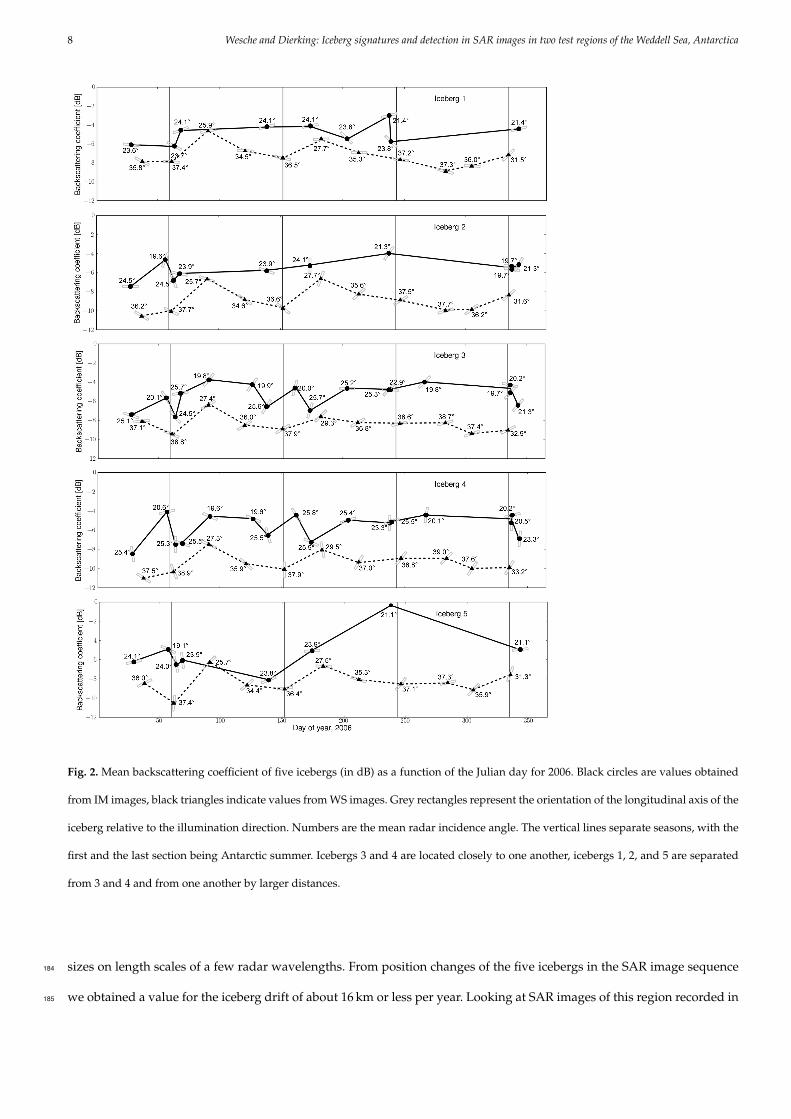
the iceberg relative to the radar look direction. Five icebergs of different sizes (between 4 km2 and 11 km2) and shapes172
were selected, which could be identified in most images of the image sequence. The results are shown in Figure 2. The173
mean backscattering intensities of the five icebergs vary as a function of time and differ between the image modes (IM174
and WS). To investigate the relative contribution of different factors influencing the backscattering coefficients, a multiple175
correlation coefficient (ra.bcd) with one goal parameter (mean backscattering intensity (a)) and three independent impact176
parameters (incidence angle (b), orientation (c), and recording day (d)) was calculated. This resulted in ra.bcd = 0.11,177
which means that none of the impact parameters had a considerable influence. Relatively, the incidence angle had the178
largest impact with ra.b = −0.26. The negative value indicates that the backscattering coefficient decreases with increasing179
incidence angle. The orientation and recording day show almost no correlation with the backscattering coefficient (ra.c =180
−0.1 and ra.d = 0.12). All correlation coefficients were calculated at a significance level of 99 %. We note that in single181
cases, the backscattered radar intensity of an iceberg may vary between SAR images acquired at different look directions,182
dependent on the orientation of reflecting facets on the iceberg surface (Sandven and others, 2007). These facets are of183
8 Wesche and Dierking: Iceberg signatures and detection in SAR images in two test regions of the Weddell Sea, Antarctica
Fig. 2. Mean backscattering coefficient of five icebergs (in dB) as a function of the Julian day for 2006. Black circles are values obtained
from IM images, black triangles indicate values from WS images. Grey rectangles represent the orientation of the longitudinal axis of the
iceberg relative to the illumination direction. Numbers are the mean radar incidence angle. The vertical lines separate seasons, with the
first and the last section being Antarctic summer. Icebergs 3 and 4 are located closely to one another, icebergs 1, 2, and 5 are separated
from 3 and 4 and from one another by larger distances.
sizes on length scales of a few radar wavelengths. From position changes of the five icebergs in the SAR image sequence184
we obtained a value for the iceberg drift of about 16 km or less per year. Looking at SAR images of this region recorded in185

Wesche and Dierking: Iceberg signatures and detection in SAR images in two test regions of the Weddell Sea, Antarctica 9
the end of 2010, all icebergs can still be found. Since they are located over Berkner Bank, one possible reason for this very186
slow drift (and observed iceberg rotations) could be that they occasionally may be in contact with the sea floor.187
The sea ice backscattering coefficient changes, in particular over the transitions from freezing to melting conditions and188
vice versa. According to Haas (2001), Antarctic sea ice backscattering reveals a seasonal cycle. The radar backscattering189
coefficients are largest in late summer. Backscattering changes are caused by the metamorphosis of snow, the formation of190
ice layers in the snow, and superimposed ice. These processes result in coarser snow grain sizes and an increasing number191
of air bubbles in the near-surface layer, which increases the radar backscattering coefficients (Haas, 2001). Under such192
conditions, the intensity contrast between icebergs and sea ice would be smallest in summer.193
In order to consider a potential sensitivity of the intensity contrast to the season, we divided our data accordingly. The194
numbers of available IM-images (in parenthesis WS-mode) are 6(3) for spring, 14(2) for summer, 20(3) for autumn, and195
21(3) for winter. The numbers of identified icebergs varies between 62 in spring and 201 in winter. Huge icebergs (>10 nm,196
named and monitored by the U.S. National Ice Center) were excluded from this analysis.197
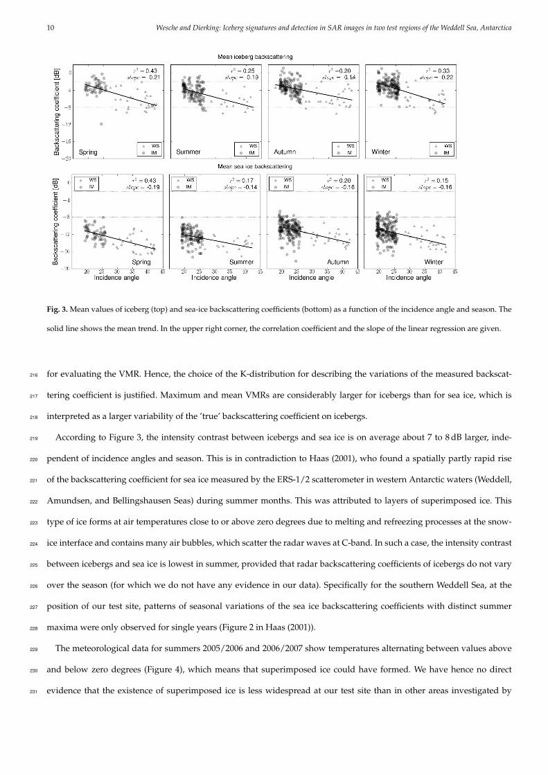
From Figure 3 it can be recognized that the observed ranges of the backscattering coefficient at a given incidence angle198
are large both for icebergs and sea ice. We attribute this to local changes of iceberg properties on the surface and in the199
subsurface layer affecting the scattering processes. In the WS images, only a few icebergs were observed at lower incidence200
angles. According to Figure 3, the average incidence angle sensitivity does not differ significantly for icebergs and sea ice.201
In general, the sensitivity is smallest for volume scattering, slightly larger for very rough surfaces and largest for smooth202
surfaces (see, e. g. Fung (1994), Chapter 2). Figure 3 indicates that on average the contribution of volume scattering or203
scattering from a very rough surfaces is dominant for icebergs and sea ice. The range of sea ice backscattering coefficients204
in Figure 3 (obtained for HH-polarization) compares well with the results of ground-based scatterometer measurements205
over rough first-year and over second-year ice reported by Drinkwater and others (1995). Their measurements were car-206
ried out at VV-polaization. For rougher surfaces and in the case of volume scattering, the difference between VV- and207
HH-polarization is only small.208
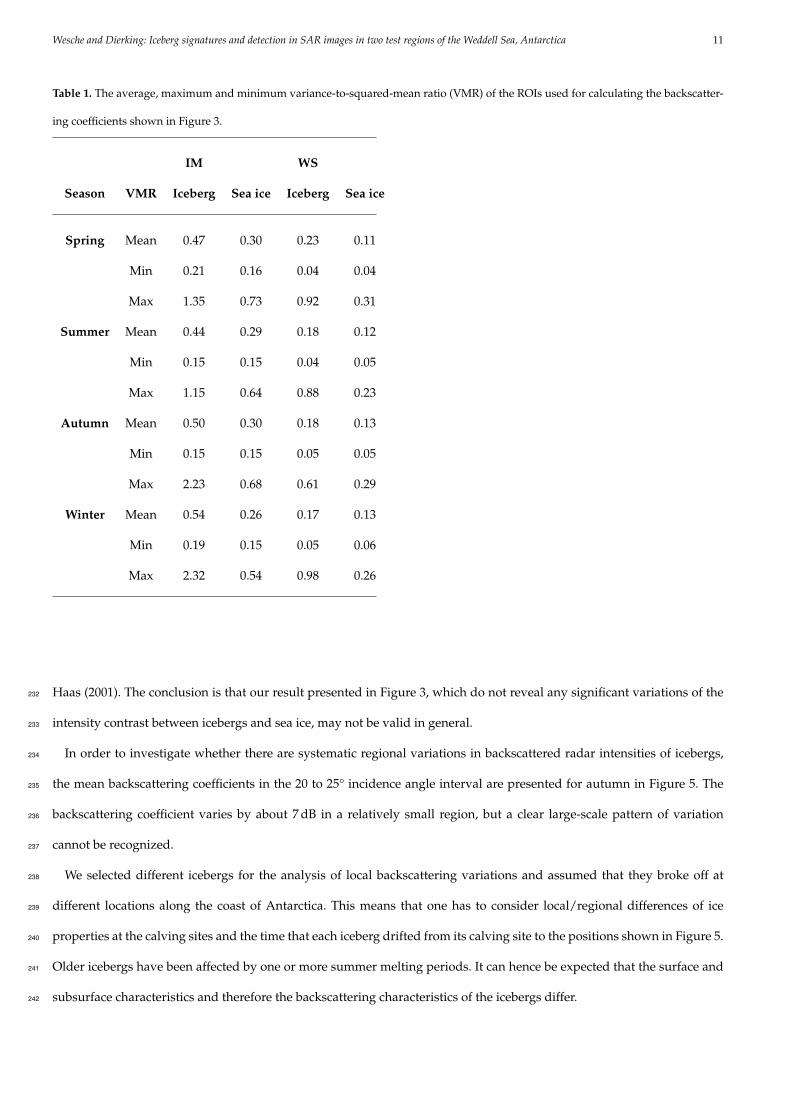
In Table 1, the average, maximum and minimum variance-to-squared-mean ratios (VMR) are presented. For the sta-209
tistical analysis, we estimated the number of looks for the pre-processed images by calculating mean and variance for210
a number of apparently texture-free areas (Equation 2). The corresponding VMRs are on average 0.16 for IM data and211
0.039 for WS mode. This agrees well with the minimum average values of the VMR listed in the table. Values close to the212
minimum indicate that the radar intensity variation is caused only by speckle. Since the maximum and mean VMRs in213
Table 1 are significantly larger than the minimum values, we have also to consider "real" variations of the backscattering214
coefficient itself (opposed to "apparent" variations due to speckle) over areas, which are of similar sizes as the ROIs used215
10 Wesche and Dierking: Iceberg signatures and detection in SAR images in two test regions of the Weddell Sea, Antarctica
Fig. 3. Mean values of iceberg (top) and sea-ice backscattering coefficients (bottom) as a function of the incidence angle and season. The
solid line shows the mean trend. In the upper right corner, the correlation coefficient and the slope of the linear regression are given.
for evaluating the VMR. Hence, the choice of the K-distribution for describing the variations of the measured backscat-216
tering coefficient is justified. Maximum and mean VMRs are considerably larger for icebergs than for sea ice, which is217
interpreted as a larger variability of the ’true’ backscattering coefficient on icebergs.218
According to Figure 3, the intensity contrast between icebergs and sea ice is on average about 7 to 8 dB larger, inde-219
pendent of incidence angles and season. This is in contradiction to Haas (2001), who found a spatially partly rapid rise220
of the backscattering coefficient for sea ice measured by the ERS-1/2 scatterometer in western Antarctic waters (Weddell,221
Amundsen, and Bellingshausen Seas) during summer months. This was attributed to layers of superimposed ice. This222
type of ice forms at air temperatures close to or above zero degrees due to melting and refreezing processes at the snow-223
ice interface and contains many air bubbles, which scatter the radar waves at C-band. In such a case, the intensity contrast224
between icebergs and sea ice is lowest in summer, provided that radar backscattering coefficients of icebergs do not vary225
over the season (for which we do not have any evidence in our data). Specifically for the southern Weddell Sea, at the226
position of our test site, patterns of seasonal variations of the sea ice backscattering coefficients with distinct summer227
maxima were only observed for single years (Figure 2 in Haas (2001)).228
The meteorological data for summers 2005/2006 and 2006/2007 show temperatures alternating between values above229
and below zero degrees (Figure 4), which means that superimposed ice could have formed. We have hence no direct230
evidence that the existence of superimposed ice is less widespread at our test site than in other areas investigated by231
Wesche and Dierking: Iceberg signatures and detection in SAR images in two test regions of the Weddell Sea, Antarctica 11
Table 1. The average, maximum and minimum variance-to-squared-mean ratio (VMR) of the ROIs used for calculating the backscatter-
ing coefficients shown in Figure 3.
IM WS
Season VMR Iceberg Sea ice Iceberg Sea ice
Spring Mean 0.47 0.30 0.23 0.11
Min 0.21 0.16 0.04 0.04
Max 1.35 0.73 0.92 0.31
Summer Mean 0.44 0.29 0.18 0.12
Min 0.15 0.15 0.04 0.05
Max 1.15 0.64 0.88 0.23
Autumn Mean 0.50 0.30 0.18 0.13
Min 0.15 0.15 0.05 0.05
Max 2.23 0.68 0.61 0.29
Winter Mean 0.54 0.26 0.17 0.13
Min 0.19 0.15 0.05 0.06
Max 2.32 0.54 0.98 0.26
Haas (2001). The conclusion is that our result presented in Figure 3, which do not reveal any significant variations of the232
intensity contrast between icebergs and sea ice, may not be valid in general.233
In order to investigate whether there are systematic regional variations in backscattered radar intensities of icebergs,234
the mean backscattering coefficients in the 20 to 25° incidence angle interval are presented for autumn in Figure 5. The235
backscattering coefficient varies by about 7 dB in a relatively small region, but a clear large-scale pattern of variation236
cannot be recognized.237
We selected different icebergs for the analysis of local backscattering variations and assumed that they broke off at238
different locations along the coast of Antarctica. This means that one has to consider local/regional differences of ice239
properties at the calving sites and the time that each iceberg drifted from its calving site to the positions shown in Figure 5.240
Older icebergs have been affected by one or more summer melting periods. It can hence be expected that the surface and241
subsurface characteristics and therefore the backscattering characteristics of the icebergs differ.242
12 Wesche and Dierking: Iceberg signatures and detection in SAR images in two test regions of the Weddell Sea, Antarctica
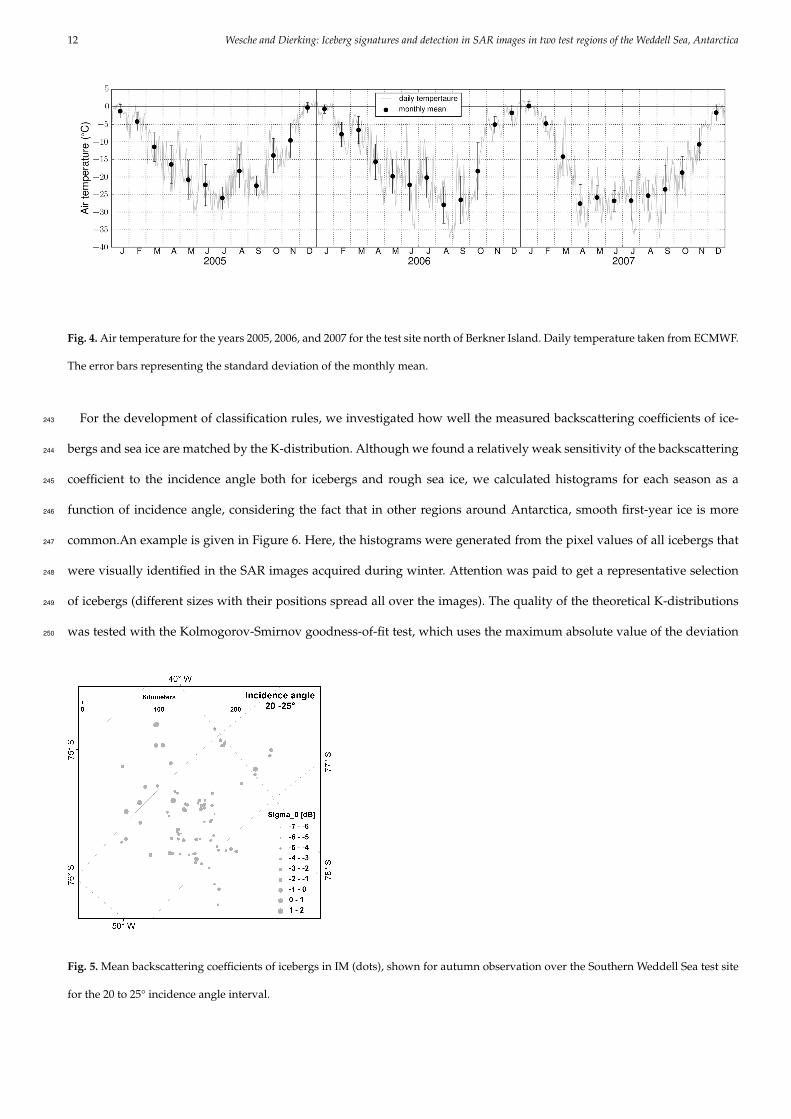
Fig. 4. Air temperature for the years 2005, 2006, and 2007 for the test site north of Berkner Island. Daily temperature taken from ECMWF.
The error bars representing the standard deviation of the monthly mean.
For the development of classification rules, we investigated how well the measured backscattering coefficients of ice-243
bergs and sea ice are matched by the K-distribution. Although we found a relatively weak sensitivity of the backscattering244
coefficient to the incidence angle both for icebergs and rough sea ice, we calculated histograms for each season as a245
function of incidence angle, considering the fact that in other regions around Antarctica, smooth first-year ice is more246
common.An example is given in Figure 6. Here, the histograms were generated from the pixel values of all icebergs that247
were visually identified in the SAR images acquired during winter. Attention was paid to get a representative selection248
of icebergs (different sizes with their positions spread all over the images). The quality of the theoretical K-distributions249
was tested with the Kolmogorov-Smirnov goodness-of-fit test, which uses the maximum absolute value of the deviation250
Fig. 5. Mean backscattering coefficients of icebergs in IM (dots), shown for autumn observation over the Southern Weddell Sea test site
for the 20 to 25° incidence angle interval.
Wesche and Dierking: Iceberg signatures and detection in SAR images in two test regions of the Weddell Sea, Antarctica 13
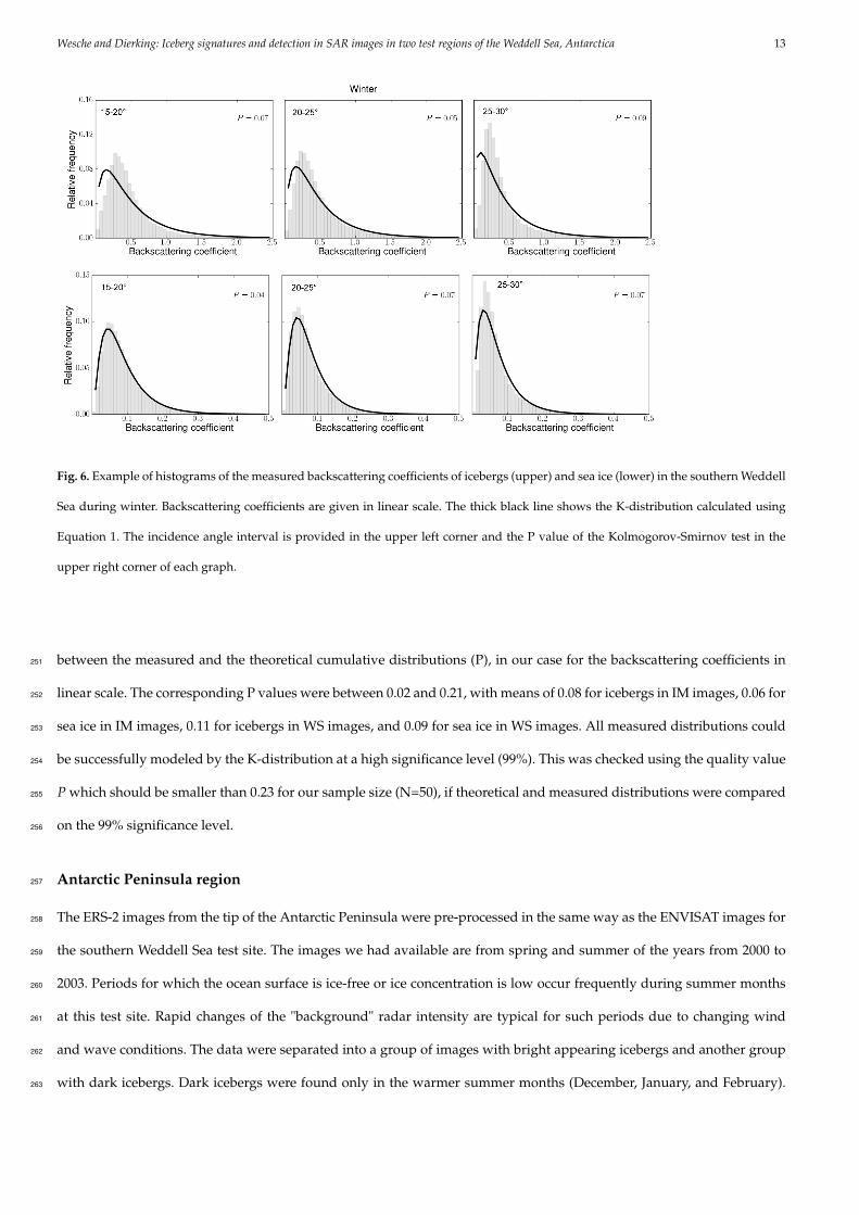
Fig. 6. Example of histograms of the measured backscattering coefficients of icebergs (upper) and sea ice (lower) in the southern Weddell
Sea during winter. Backscattering coefficients are given in linear scale. The thick black line shows the K-distribution calculated using
Equation 1. The incidence angle interval is provided in the upper left corner and the P value of the Kolmogorov-Smirnov test in the
upper right corner of each graph.
between the measured and the theoretical cumulative distributions (P), in our case for the backscattering coefficients in251
linear scale. The corresponding P values were between 0.02 and 0.21, with means of 0.08 for icebergs in IM images, 0.06 for252
sea ice in IM images, 0.11 for icebergs in WS images, and 0.09 for sea ice in WS images. All measured distributions could253
be successfully modeled by the K-distribution at a high significance level (99%). This was checked using the quality value254
P which should be smaller than 0.23 for our sample size (N=50), if theoretical and measured distributions were compared255
on the 99% significance level.256
Antarctic Peninsula region257
The ERS-2 images from the tip of the Antarctic Peninsula were pre-processed in the same way as the ENVISAT images for258
the southern Weddell Sea test site. The images we had available are from spring and summer of the years from 2000 to259
2003. Periods for which the ocean surface is ice-free or ice concentration is low occur frequently during summer months260
at this test site. Rapid changes of the "background" radar intensity are typical for such periods due to changing wind261
and wave conditions. The data were separated into a group of images with bright appearing icebergs and another group262
with dark icebergs. Dark icebergs were found only in the warmer summer months (December, January, and February).263
14 Wesche and Dierking: Iceberg signatures and detection in SAR images in two test regions of the Weddell Sea, Antarctica
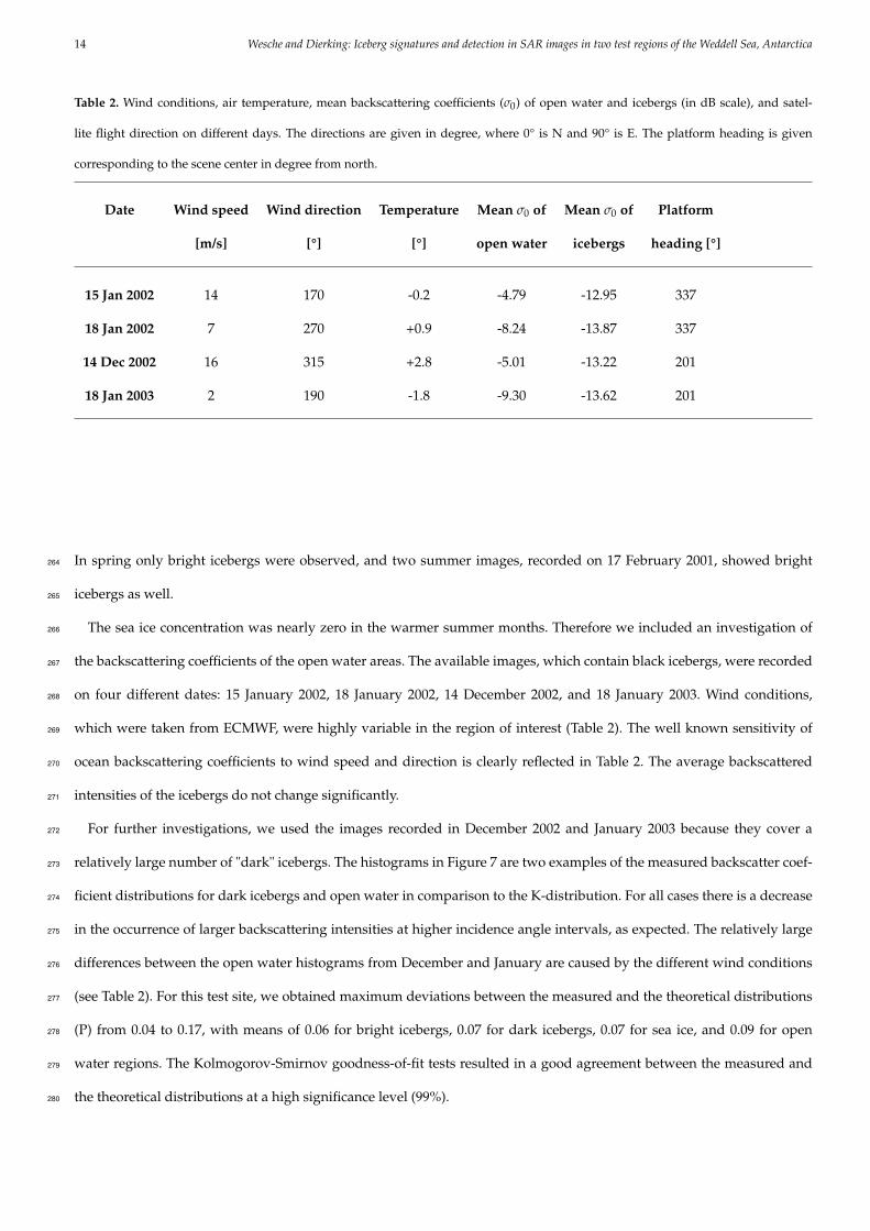
Table 2. Wind conditions, air temperature, mean backscattering coefficients (σ0) of open water and icebergs (in dB scale), and satel-
lite flight direction on different days. The directions are given in degree, where 0° is N and 90° is E. The platform heading is given
corresponding to the scene center in degree from north.
Date Wind speed Wind direction Temperature Mean σ0 of Mean σ0 of Platform
[m/s] [°] [°] open water icebergs heading [°]
15 Jan 2002 14 170 -0.2 -4.79 -12.95 337
18 Jan 2002 7 270 +0.9 -8.24 -13.87 337
14 Dec 2002 16 315 +2.8 -5.01 -13.22 201
18 Jan 2003 2 190 -1.8 -9.30 -13.62 201
In spring only bright icebergs were observed, and two summer images, recorded on 17 February 2001, showed bright264
icebergs as well.265
The sea ice concentration was nearly zero in the warmer summer months. Therefore we included an investigation of266
the backscattering coefficients of the open water areas. The available images, which contain black icebergs, were recorded267
on four different dates: 15 January 2002, 18 January 2002, 14 December 2002, and 18 January 2003. Wind conditions,268
which were taken from ECMWF, were highly variable in the region of interest (Table 2). The well known sensitivity of269
ocean backscattering coefficients to wind speed and direction is clearly reflected in Table 2. The average backscattered270
intensities of the icebergs do not change significantly.271
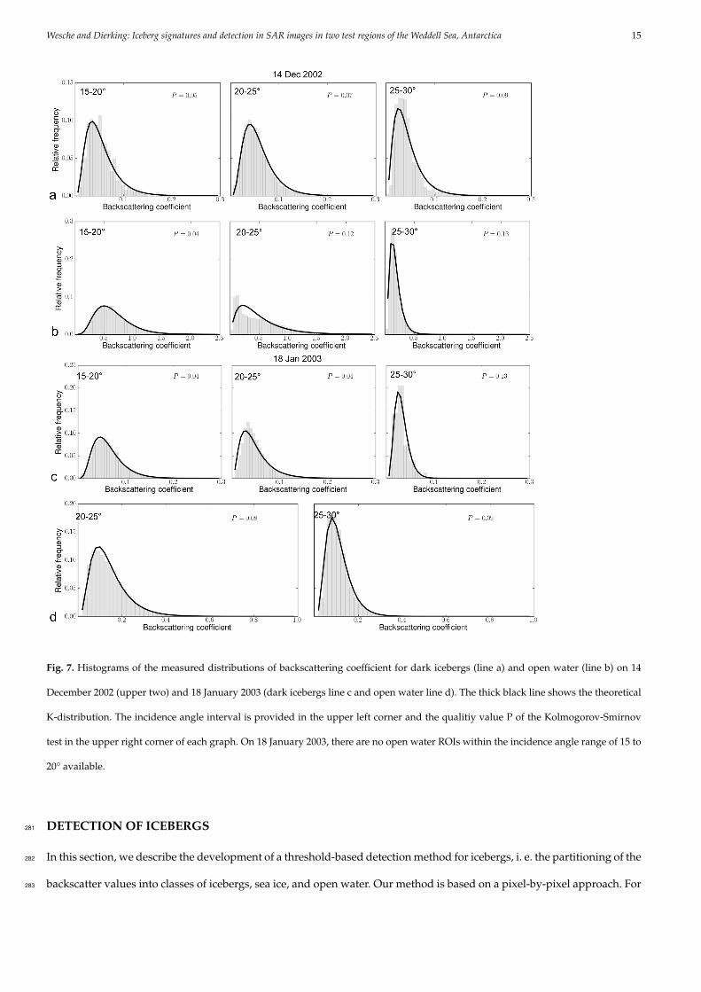
For further investigations, we used the images recorded in December 2002 and January 2003 because they cover a272
relatively large number of "dark" icebergs. The histograms in Figure 7 are two examples of the measured backscatter coef-273
ficient distributions for dark icebergs and open water in comparison to the K-distribution. For all cases there is a decrease274
in the occurrence of larger backscattering intensities at higher incidence angle intervals, as expected. The relatively large275
differences between the open water histograms from December and January are caused by the different wind conditions276
(see Table 2). For this test site, we obtained maximum deviations between the measured and the theoretical distributions277
(P) from 0.04 to 0.17, with means of 0.06 for bright icebergs, 0.07 for dark icebergs, 0.07 for sea ice, and 0.09 for open278
water regions. The Kolmogorov-Smirnov goodness-of-fit tests resulted in a good agreement between the measured and279
the theoretical distributions at a high significance level (99%).280
Wesche and Dierking: Iceberg signatures and detection in SAR images in two test regions of the Weddell Sea, Antarctica 15
Fig. 7. Histograms of the measured distributions of backscattering coefficient for dark icebergs (line a) and open water (line b) on 14
December 2002 (upper two) and 18 January 2003 (dark icebergs line c and open water line d). The thick black line shows the theoretical
K-distribution. The incidence angle interval is provided in the upper left corner and the qualitiy value P of the Kolmogorov-Smirnov
test in the upper right corner of each graph. On 18 January 2003, there are no open water ROIs within the incidence angle range of 15 to
20° available.
DETECTION OF ICEBERGS281
In this section, we describe the development of a threshold-based detection method for icebergs, i. e. the partitioning of the282
backscatter values into classes of icebergs, sea ice, and open water. Our method is based on a pixel-by-pixel approach. For283
16 Wesche and Dierking: Iceberg signatures and detection in SAR images in two test regions of the Weddell Sea, Antarctica
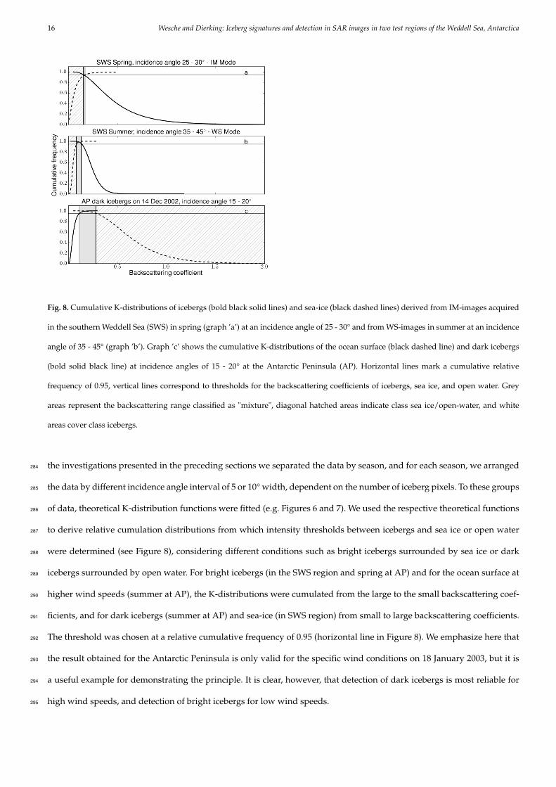
Fig. 8. Cumulative K-distributions of icebergs (bold black solid lines) and sea-ice (black dashed lines) derived from IM-images acquired
in the southern Weddell Sea (SWS) in spring (graph ’a’) at an incidence angle of 25 - 30° and from WS-images in summer at an incidence
angle of 35 - 45° (graph ’b’). Graph ’c’ shows the cumulative K-distributions of the ocean surface (black dashed line) and dark icebergs
(bold solid black line) at incidence angles of 15 - 20° at the Antarctic Peninsula (AP). Horizontal lines mark a cumulative relative
frequency of 0.95, vertical lines correspond to thresholds for the backscattering coefficients of icebergs, sea ice, and open water. Grey
areas represent the backscattering range classified as "mixture", diagonal hatched areas indicate class sea ice/open-water, and white
areas cover class icebergs.
the investigations presented in the preceding sections we separated the data by season, and for each season, we arranged284
the data by different incidence angle interval of 5 or 10° width, dependent on the number of iceberg pixels. To these groups285
of data, theoretical K-distribution functions were fitted (e.g. Figures 6 and 7). We used the respective theoretical functions286
to derive relative cumulation distributions from which intensity thresholds between icebergs and sea ice or open water287
were determined (see Figure 8), considering different conditions such as bright icebergs surrounded by sea ice or dark288
icebergs surrounded by open water. For bright icebergs (in the SWS region and spring at AP) and for the ocean surface at289
higher wind speeds (summer at AP), the K-distributions were cumulated from the large to the small backscattering coef-290
ficients, and for dark icebergs (summer at AP) and sea-ice (in SWS region) from small to large backscattering coefficients.291
The threshold was chosen at a relative cumulative frequency of 0.95 (horizontal line in Figure 8). We emphasize here that292
the result obtained for the Antarctic Peninsula is only valid for the specific wind conditions on 18 January 2003, but it is293
a useful example for demonstrating the principle. It is clear, however, that detection of dark icebergs is most reliable for294
high wind speeds, and detection of bright icebergs for low wind speeds.295

Wesche and Dierking: Iceberg signatures and detection in SAR images in two test regions of the Weddell Sea, Antarctica 17
Fig. 9. Mean difference of ’0.95-thresholds’ (at linear scale) between icebergs and sea ice for each season at the southern Weddell Sea test
site. Circles representing IM images and triangles WS images. The color code shows the incidence angle range.
The range of backscattering coefficients shown in Figure 8 was separated into three different classes: (1) icebergs (white296
area), (2) mixture (grey area), and (3) sea ice (diagonal hatched area). In general, the positions of the 0.95 relative frequency297
threshold are different for icebergs and sea ice/open water. The differences between the 0.95-thresholds for icebergs and298
for sea ice are shown for all incidence angle intervals over a whole seasonal cycle for the Weddell Sea test site in Figure 9,299
using IM and WS data. Positive values are optimal for detection. They indicate that the number of iceberg and sea ice300
pixels with identical values of the backscattering coefficient is small (Figure 8b and c). Negative differences mean that301
the 0.95-cumulative frequency level of the icebergs is reached at lower backscattering coefficients than the one for sea-ice302
(Figure 8a). Since the final iceberg-threshold is determined by the upper intensity limit of the mixture zone (in case of303
bright icebergs), it corresponds to a cumulative frequency level less than 0.95. This means that more sea ice pixel and304
less iceberg pixels are classified correctly. The results presented in Figure 9 reveal a weak advantage for iceberg detection305
when spring and summer data are used. We assume that the larger negative threshold differences found in the autumn and306
winter IM-images are related to "unfavorable" sea ice conditions characterized by patterns of relatively high backscattering307
intensities due to sea ice deformation. Overlaps between classes ’icebergs’ and ’sea ice’ were in general smaller in the308
WS-images than in IM data. This may be due to a ’smearing’ effect on the backscattering signature of narrow sea ice309
deformation patterns within one pixel of the coarse-resolution image. The threshold difference is in general dependent on310
the intensity contrast between icebergs and sea ice and hence on local and temporal variations of sea ice conditions.311
As a next step, the derived thresholds were applied to all images available for our study, on a pixel-by-pixel basis, con-312
sidering the respective incidence angle range. Each pixel was then marked by a number indicating the class. Figure 10a313
shows the zoom-in of an unfiltered SAR image covering one large iceberg surrounded by sea ice of different age and a314
lead, which either was a calm open water surface or thin new ice (black in Figure 10a and e). The different grey tones315
in Figure 10a correspond to radar intensities given as sigma nought in linear scale. The result after applying the detec-316
18 Wesche and Dierking: Iceberg signatures and detection in SAR images in two test regions of the Weddell Sea, Antarctica
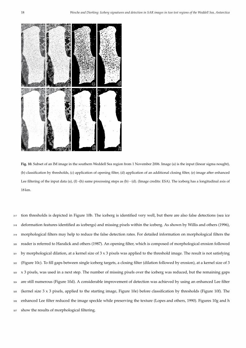
Fig. 10. Subset of an IM image in the southern Weddell Sea region from 1 November 2006. Image (a) is the input (linear sigma nought),
(b) classification by thresholds, (c) application of opening filter, (d) application of an additional closing filter, (e) image after enhanced
Lee filtering of the input data (a), (f) -(h) same processing steps as (b) - (d). (Image credits: ESA). The iceberg has a longitudinal axis of
18 km.
tion thresholds is depicted in Figure 10b. The iceberg is identified very well, but there are also false detections (sea ice317
deformation features identified as icebergs) and missing pixels within the iceberg. As shown by Willis and others (1996),318
morphological filters may help to reduce the false detection rates. For detailed information on morphological filters the319
reader is referred to Haralick and others (1987). An opening filter, which is composed of morphological erosion followed320
by morphological dilation, at a kernel size of 3 x 3 pixels was applied to the threshold image. The result is not satisfying321
(Figure 10c). To fill gaps between single iceberg targets, a closing filter (dilation followed by erosion), at a kernel size of 3322
x 3 pixels, was used in a next step. The number of missing pixels over the iceberg was reduced, but the remaining gaps323
are still numerous (Figure 10d). A considerable improvement of detection was achieved by using an enhanced Lee filter324
(kernel size 3 x 3 pixels, applied to the starting image, Figure 10e) before classification by thresholds (Figure 10f). The325
enhanced Lee filter reduced the image speckle while preserving the texture (Lopes and others, 1990). Figures 10g and h326
show the results of morphological filtering.327

Wesche and Dierking: Iceberg signatures and detection in SAR images in two test regions of the Weddell Sea, Antarctica 19
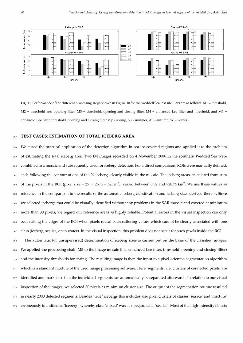
The performance of the different processing steps was tested by comparing the results of the threshold-classified and328
filtered images with the manually chosen icebergs, sea ice, and open-water ROIs as reference. The result of this comparison329
for the Weddell Sea test site is shown in Figure 11 separately for the different seasons. The height of the bars shown in330
Figure 11 gives the percentage of the correctly classified iceberg and sea ice pixels, respectively. This means, for example,331
that in IM (WS) images, on average 2.6 (5.9) percent of the iceberg pixels are erroneously classified as sea ice during332
summer, and 8.7 (6.7) percent during winter, using the processing chain M5. In the case of sea ice, the corresponding333
fractions of pixels classified as iceberg are 1.1 (16.7) percent for summer and 2.9 (2.5) percent for winter data. When334
morphological filters are applied, wrongly classified areas of small size are already removed. It is easy to see that the sea335
ice classification is more accurate in the IM-images than in the WS-data. This agrees with the result presented in Figure 9.336
There, negative threshold differences indicate that the thresholds are shifted towards higher intensity values than the ones337
corresponding to the 0.95-cumulative frequency level of the icebergs. However, for the result presented in Figure 11 the338
spatial distribution of the pixel is important in the cases in which filters are applied, so that only the M1-case can directly339
be compared to Figure 9.340
In the case of icebergs, the application of the opening filter on the threshold images, without first applying the enhanced341
Lee filter for speckle reduction, deteriorates the detection performance (M1 versus M2-bars in Figure 11). The successive342
use of the closing filter improves the result (M3-bars in Figure 11). If an enhanced Lee filter is employed before classifica-343
tion, the detection accuracy increases (M1 versus M4-bars, Figure 11). However, morphological filtering does not improve344
the result (M4 versus M5-bars, Figure 11). In the case of sea ice, the application of morphological filters on the threshold345
images, without a preceding enhanced Lee filter, was benefical (M2 and M3-bars in Figure 11). The enhanced Lee filter346
increased the classification accuracy only slightly (M4 versus M1-bars in Figure 11) and the gain of the morphological347
filters was only marginal (M5 versus M4-bars in Figure 11). The results indicate that in general, it is sufficient to apply348
the enhanced Lee filter followed by a threshold operation to separate icebergs and sea ice. The only exception was found349
for sea ice in WS-images, for which the morphological filtering applied on M1-images leads to a considerable improve-350
ment of the classification accuracy in particular in spring and summer data. For IM-images, spring and summer reveal351
slightly better classification results. For the WS-data, we have no clear evidence for a particular season being optimal352
for iceberg detection. In summary we found that the application of different filters on the input SAR image influences353
the classification result, in some cases considerably. However, we could not establish a generally valid optimal filtering354
approach, which comprises IM- and WS-images and different sea ice conditions, and, in the case of open water, different355
wind condiations.356
20 Wesche and Dierking: Iceberg signatures and detection in SAR images in two test regions of the Weddell Sea, Antarctica
Fig. 11. Performance of the different processing steps shown in Figure 10 for the Weddell Sea test site. Bars are as follows: M1 = threshold,
M2 = threshold and opening filter, M3 = threshold, opening and closing filter, M4 = enhanced Lee filter and threshold, and M5 =
enhanced Lee filter, threshold, opening and closing filter. (Sp - spring, Su - summer, Au - autumn, Wi - winter).
TEST CASES: ESTIMATION OF TOTAL ICEBERG AREA357
We tested the practical application of the detection algorithm in sea ice covered regions and applied it to the problem358
of estimating the total iceberg area. Two IM images recorded on 4 November 2006 in the southern Weddell Sea were359
combined in a mosaic and subsequently used for iceberg detection. For a direct comparison, ROIs were manually defined,360
each following the contour of one of the 29 icebergs clearly visible in the mosaic. The iceberg areas, calculated from sum361
of the pixels in the ROI (pixel size = 25 × 25 m = 625 m2), varied between 0.02 and 728.75 km2. We use these values as362
reference in the comparison to the results of the automatic iceberg classification and iceberg sizes derived thereof. Since363
we selected icebergs that could be visually identified without any problems in the SAR mosaic and covered at minimum364
more than 30 pixels, we regard our reference areas as highly reliable. Potential errors in the visual inspection can only365
occur along the edges of the ROI when pixels reveal backscattering values which cannot be clearly associated with one366
class (iceberg, sea ice, open water). In the visual inspection, this problem does not occur for such pixels inside the ROI.367
The automtatic (or unsupervised) determination of iceberg sizes is carried out on the basis of the classified images.368
We applied the processing chain M5 to the image mosaic (i. e. enhanced Lee filter, threshold, opening and closing filter)369
and the intensity thresholds for spring. The resulting image is then the input to a pixel-oriented segmentation algorithm370
which is a standard module of the used image processing software. Here, segments, i. e. clusters of connected pixels, are371
identified and marked so that the individual segments can automatically be separated afterwards. In relation to our visual372
inspection of the images, we selected 30 pixels as minimum cluster size. The output of the segmenation routine resulted373
in nearly 2000 detected segments. Besides "true" icebergs this includes also pixel clusters of classes ’sea ice’ and ’mixture’374
erroneously identified as ’iceberg’, whereby class ’mixed’ was also regarded as ’sea ice’. Most of the high-intensity objects375

Wesche and Dierking: Iceberg signatures and detection in SAR images in two test regions of the Weddell Sea, Antarctica 21
in the SAR image are deformation zones (ridges, rubble, brash ice) in the sea ice cover, with areas between 0.02 and 9.7 km2376
(calculated from the sum of clustered pixels). On the one hand, the automated approach "adds" contributions from false377
detections to the total sum of iceberg pixels, on the other hand, it subtracts "true" iceberg pixels, which are classified as378
sea ice. Two of the 29 manually detected icebergs, with areas of 0.02 km2 and 0.13 km2, respectively, were not detected at379
all in the unsupervised classification. Comparing the automatically determined iceberg areas to the manual reference, we380
found both negative and positive deviations, but on average, the iceberg size were overestimated by 10 ± 21 percent. A381
value of 20 percent was obtained by Young and others (1998), who used an edge detection approach for identification of382
icebergs.383
For the calculation of the total iceberg area from the classification results of the unsupervised threshold algorithm,384
objects with sizes less than 0.02 km2 (corresponding to 30 image pixels) were regarded as false detections. We cannot385
exclude that some of these objects are indeed icebergs. In the study by Young and others (1998), a reliable detection in386
ERS-1 images (VV-polarization) was possible for icebergs with areas larger than 0.06 km2, corresponding to six image387
pixels at a size of 100 m × 100 m. Differences in the sea ice conditions are the reason why we had to select a threshold388
of 30 image pixels of 25 m in size for the minimum detectable size of the icebergs. In the study by Young and others389
(1998), the icebergs were mostly surrounded by a background of first-year ice and partly by open water and thin ice.390
The backscatter value of the background was less than -10.5 dB in 99 percent of all cases. As Figure 3 above reveals, the391
observed backscattering coefficients of sea ice at our test site can be as large as -7 dB at HH-polarization using IM-mode392
data at an incidence angle range comparable to ERS-1. This is attributed to a rough ice surface and the presence of multi-393
year ice for which the backscattering coefficients can be larger than -7 dB at VV-polarization (Young and others, 1998). For394
rougher ice, VV- and HH-polarization differ only slightly, as already mentioned above.395
The size distribution of targets revealing a high backscattering coefficient (sea ice deformation zones and icebergs) is396
shown in Figure 12(left). It is obvious that for this special case, the total areas of smaller icebergs are critically overesti-397
mated.398
Further tests for iceberg detection were carried out using WS images acquired over the Weddell Sea test site. In Fig-399
ure 13a, an example recorded on 1 November 2006 is shown. On the basis of the results on the effect of different filters400
presented above, the test data were processed by applying opening and closing filter on the threshold image (M3, Fig-401
ure 11). All visible icebergs were manually marked by ROIs following the iceberg margins. In the center, the iceberg A23-A402
is visible. The A23-A is a fragment of A23, which calved from the Filcher-Ronne-Ice-Shelf in 1986. The A23-A broke off403
in 1991 and is aground since then. For determining the intensity thresholds for classification, the A23-A and A-27 (only a404
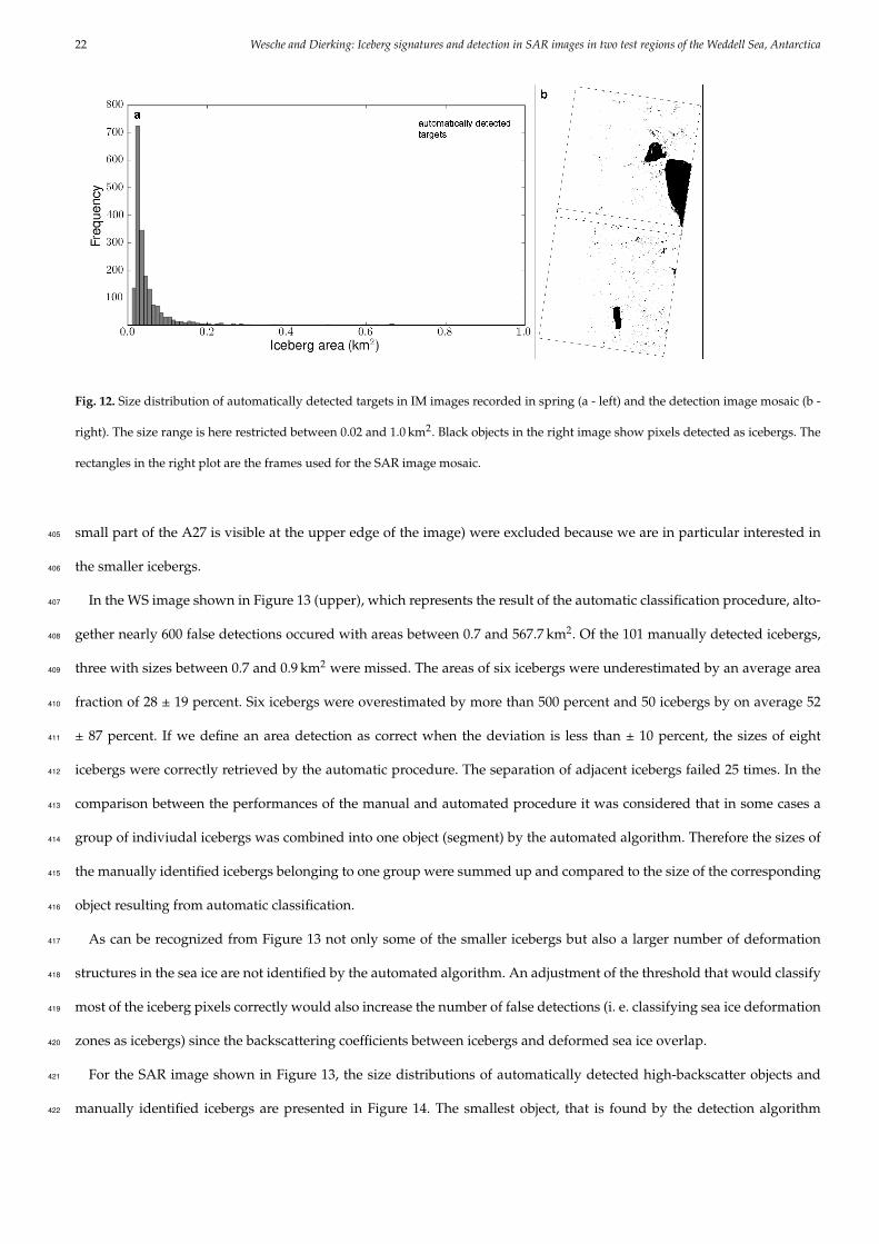
22 Wesche and Dierking: Iceberg signatures and detection in SAR images in two test regions of the Weddell Sea, Antarctica
Fig. 12. Size distribution of automatically detected targets in IM images recorded in spring (a - left) and the detection image mosaic (b -
right). The size range is here restricted between 0.02 and 1.0 km2. Black objects in the right image show pixels detected as icebergs. The
rectangles in the right plot are the frames used for the SAR image mosaic.
small part of the A27 is visible at the upper edge of the image) were excluded because we are in particular interested in405
the smaller icebergs.406
In the WS image shown in Figure 13 (upper), which represents the result of the automatic classification procedure, alto-407
gether nearly 600 false detections occured with areas between 0.7 and 567.7 km2. Of the 101 manually detected icebergs,408
three with sizes between 0.7 and 0.9 km2 were missed. The areas of six icebergs were underestimated by an average area409
fraction of 28 ± 19 percent. Six icebergs were overestimated by more than 500 percent and 50 icebergs by on average 52410
± 87 percent. If we define an area detection as correct when the deviation is less than ± 10 percent, the sizes of eight411
icebergs were correctly retrieved by the automatic procedure. The separation of adjacent icebergs failed 25 times. In the412
comparison between the performances of the manual and automated procedure it was considered that in some cases a413
group of indiviudal icebergs was combined into one object (segment) by the automated algorithm. Therefore the sizes of414
the manually identified icebergs belonging to one group were summed up and compared to the size of the corresponding415
object resulting from automatic classification.416
As can be recognized from Figure 13 not only some of the smaller icebergs but also a larger number of deformation417
structures in the sea ice are not identified by the automated algorithm. An adjustment of the threshold that would classify418
most of the iceberg pixels correctly would also increase the number of false detections (i. e. classifying sea ice deformation419
zones as icebergs) since the backscattering coefficients between icebergs and deformed sea ice overlap.420
For the SAR image shown in Figure 13, the size distributions of automatically detected high-backscatter objects and421
manually identified icebergs are presented in Figure 14. The smallest object, that is found by the detection algorithm422
Wesche and Dierking: Iceberg signatures and detection in SAR images in two test regions of the Weddell Sea, Antarctica 23
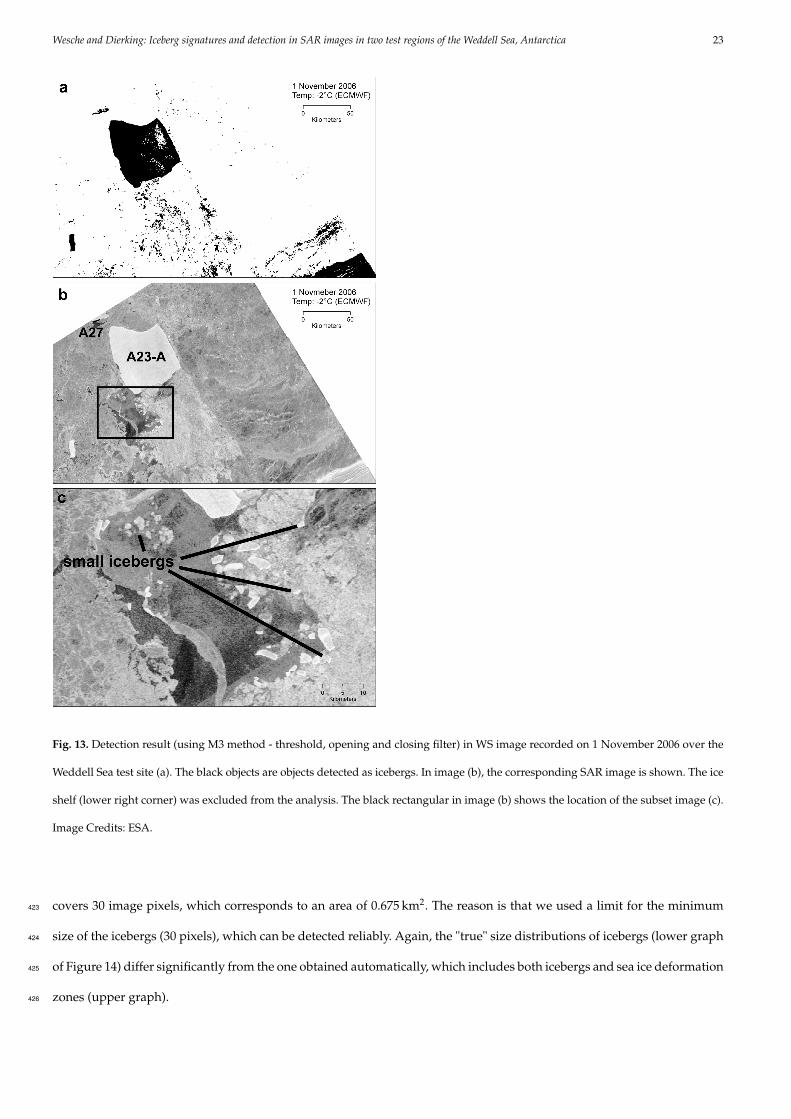
Fig. 13. Detection result (using M3 method - threshold, opening and closing filter) in WS image recorded on 1 November 2006 over the
Weddell Sea test site (a). The black objects are objects detected as icebergs. In image (b), the corresponding SAR image is shown. The ice
shelf (lower right corner) was excluded from the analysis. The black rectangular in image (b) shows the location of the subset image (c).
Image Credits: ESA.
covers 30 image pixels, which corresponds to an area of 0.675 km2. The reason is that we used a limit for the minimum423
size of the icebergs (30 pixels), which can be detected reliably. Again, the "true" size distributions of icebergs (lower graph424
of Figure 14) differ significantly from the one obtained automatically, which includes both icebergs and sea ice deformation425
zones (upper graph).426

24 Wesche and Dierking: Iceberg signatures and detection in SAR images in two test regions of the Weddell Sea, Antarctica
Fig. 14. Size distributions of automatically (M3 - threshold, opening and closing filter) detected objects (upper) and manually detected
icebergs (lower) in WS image recorded on 1 November 2006. The x-axis was cut off at 5 km2.
CONCLUSION427
We investigated the detection of icebergs in SAR images from the Weddell Sea, focussing specifically on smaller icebergs428
from less than 10 nm side length down to sizes of 0.02 km2. We had ENVISAT ASAR IM- and WS mode data at HH-429
polarization available, acquired north of Berkner Island during 2006, and ERS-2 data at VV-polarization from a region430
east of the tip of the Antarctic Peninsula that were taken in spring and summer months from 2000 to 2003.431
Based on the SAR data, we analyzed the influence of different parameters on variations of the radar intensity backscat-432
tered from icebergs. These parameters were the radar incidence angle, the orientation of the iceberg relative to the radar433
look direction, and the season of data acquisition. Relative to the other parameters, the sensitivity to the radar incidence434
angle was largest, but the absolute value of the correlation coefficient was small. This indicates that for our test cases,435
backscattering from the ice volume or from a very rough surface was dominant. Systematic spatial or temporal variations436
of iceberg signatures could not be recognized.437
For our southern Weddell Sea test site we did not find any significant seasonal differences in the intensity contrast438
between icebergs and sea ice. We observed that backscattering coefficient of icebergs and sea ice were slightly lower during439
spring and summer. This is in contradiction to scatterometer data of seasonal backscatter variations of sea ice around West-440
Antarctica with summer maxima at many locations and over a number of years (Haas, 2001). Thus, it is possible that our441
result is not generally valid. Considering our finding that iceberg radar intensities do not reveal a seasonal maximum,442
iceberg identification may hence often be more difficult in summer. The recognition of icebergs in the open ocean and443
in low-concentration sea ice depends strongly on the meteorological conditions and the ocean wave field. The radar444
signatures of open water areas vary with changing wind conditions (speed, direction), the ones of sea ice and icebergs445
change drastically at the onset of melting (e. g. "black" icebergs observed close to the Antarctic Peninsula). This item is446
further discussed at the end of this section.447

Wesche and Dierking: Iceberg signatures and detection in SAR images in two test regions of the Weddell Sea, Antarctica 25
We found that a K-distribution matches well with the observed radar intensity variations of icebergs, sea ice, and open448
water. By opposing the cumulative K-distributions of icebergs and sea ice or water separately for the four seasons we449
established radar intensity thresholds as a function of incidence angle range (excluding huge named icebergs). We did450
not observe a robust temporal sensitivity of the differences between iceberg and sea ice backscattering in our data. Except451
the fact that the IM-mode data make it possible to identify smaller icebergs (down to approximately 0.02 km2 compared452
to 0.7 km2 for WS-mode), the results for radar scattering characteristics from IM-mode compared well with the WS-mode453
(images were acquired at different days).454
The overall performance for iceberg detection in sea ice (i. e. considering iceberg pixels classified as sea ice and sea455
ice pixels classified as iceberg) is similar at both coarser and higher spatial resolution (WS: 150 m versus 30 m for IM).456
Significant differences could not be affirmed (Figure 11). We investigated how the processing of the images before clas-457
sification, i. e. the application of speckle- and morphological filtering affects the iceberg identification. We found that the458
classification accuracy increases when the enhanced Lee-filter is used. In this case, a successive application of morpholog-459
ical (opening and closing) filters did not reveal significant improvements. If the Lee-filter was not used, morphological460
filtering reduced the accuracy of iceberg detection but improved sea ice classification. An optimal, generally valid filtering461
procedure cannot be recommended at this point except the application of speckle filters.462
Finally, we presented detailed examples of detection / classification results using both IM and WS-mode data from463
the test site north of Berkner Island. We could demonstrate that adverse sea ice conditions (i. e. the presence of strong464
deformation patterns) have a large influence on the detection result and any parameters derived based on the classified465
image (with classes ’iceberg’ and ’background’).466
Optimal situations for iceberg detection are low wind speed and freezing conditions. By combining model simulations467
of ocean radar signatures as a function of wind speed and direction with a larger number of data than we had available for468
this study, a more detailed method for robust detection of icebergs in open water areas could be developed. With smooth469
new and first-year ice as background, icebergs are easier to recognize. This suggests early winter as the optimum season.470
However, if ice formation takes place on a rough water surface, wide belts of pancake ice may develop. Thin smooth471
ice is rafted by the influence of wind forces, and ice ridges may form in slightly thicker first-year ice. In some regions472
around Antarctica, the ice cover is perennial, with complex surface structures that may strongly scatter the incoming473
radar waves. In all these cases, the backscattered radar intensity exceeds partly significantly the intensity level typical for474
smooth first-year ice. For a reliable iceberg census, a manual verification stage after automatic iceberg detection, as also475
applied by Young and others (1998), may hence be inevitable in case of critical sea ice conditions. The results of initial476
automated iceberg detection are nevertheless highly valuable since they support any subsequent manual analysis. An477
26 Wesche and Dierking: Iceberg signatures and detection in SAR images in two test regions of the Weddell Sea, Antarctica
improvement of the approach presented in this paper could be to use quantitative measures of sea ice conditions (the478
occurrence and timing of which may vary from year to year at a given location) and to determine those conditions, which479
are better suited for iceberg detection than others. Hence, a two-step procedure is required: in the first step, regionally480
sea ice conditions are analyzed, and if suitable, iceberg detection is carried out in the next step. For regions which reveal481
long-lasting unfavorable conditions, the use of different radar bands (L, X) and different polarization modes may improve482
the situation. This will be investigated in further studies.483
ACKNOWLEDGEMENTS484
The SAR images were provided by ESA for the Cat-1 project C1P.5024. Funding was provided by DFG-Priority Programme485
1158 - Antarctic research with comparative investigations in Arctic ice areas (DI 909/3-1 and -2) which we gratefully486
acknowledge. For this paper, Manfred Lange acted as Chief Scientific Editor. We would like to thank Neal Young and two487
anonymous reviewer for their constructive and helpful comments.488
References489
Drinkwater, M. R., R. Hosseinmostafa and P. Gogineni, 1995. C-band backscatter measurements of winter sea-ice in the490
Weddell Sea, Antarctica, International Journal of Remote Sensing, 16(17), 3365–3389.491
Fung, A. K., 1994. Mircowave scattering and emission models and their applications, Artech House, Norwood, MA 02062.492
Gray, A. L. and L. D. Arsenault, 1991. Time-delayed reflections in L-band synthetic aperature radar imaginary of icebergs,493
IEEE Geoscience and Remote Sensing, 29(2), 284–291.494
Gutt, J. and A. Starmans, 2001. Quantification of iceberg impact and benthic recolonisation patterns in the Weddell Sea495
(Antarctica), Polar Biology, 24, 615–619.496
Haas, C., 2001. The seasonal cycle of ERS scatterometer signatures over perennial Antarctic sea ice and associated surface497
ice properties and processes, Annals of Glaciology, 33(1), 69–73.498
Haralick, R. M., S. R. Sternberg and X. H. Zhuang, 1987. Image-analysis using mathematical morphology, IEEE Transactions499
on Pattern Analysis and Machine Intelligence, 9(4), 532–550.500
Haran, T., J. Bohlander, T. Scambos, T. Painter and M. Fahnestock, 2006. MODIS mosaic of Antarctica (MOA) image map,501
Boulder, Colorado, National Snow and Ice Data Center, Digital media.502
Jackson, C. R. and J. R. Apel, 2005. Synthetic aperture radar marine user’s manual, Commerce Dept., NOAA, National503
Environmental Satellite, Data, and Information Service, Office of Research and Applications.504
Jacobs, S. S., H. H. Hellmer, C. S. M. Doake, A. Jenkins and R. M. Frolich, 1992. Melting of ice shelves and the mass balance505
of Antarctica, Journal of Glaciology, 38(130), 375–387.506

Wesche and Dierking: Iceberg signatures and detection in SAR images in two test regions of the Weddell Sea, Antarctica 27
Jenkins, A., 1999. The impact of melting ice on ocean waters, Journal of Physical Oceanography, 29, 2370–2381.507
Lopes, A., R. Touzi and E. Nezry, 1990. Adaptive speckle filters and scene heterogeneity, IEEE Transactions on Geoscience508
and Remote Sensing, 28(6), 992–1000.509
Oliver, C. and S. Quegan, 1998. Understanding Synthetic Aperture Radar Images, Artech House Remote Sensing Library,510
Boston Mass: Artech House, Boston.511
Paterson, W.S.B., 1994. The physics of glaciers, Butterworth Heinemann, Oxford, UK, 3 ed.512
Power, D., J. Youden, K. Lane, C. Randell and D. Flett, 2001. Iceberg detection capabilities of RADARSAT Synthetic Aper-513
ture Radar, Canadian Journal of Remote Sensing, 27(5), 476–486.514
Redding, N., 1999. Estimating the parameters of the K distribution in the intensity domain, DSTO Electronics and515
Surveilance Laboratory, South Australia, Report DSTO-TR-0839, 1–60.516
Sandven, S., M. Babiker and K. Kloster, 2007. Iceberg observations in the Barents Sea by radar and optical satellite images,517
Proceedings of the ENVISAT Symposium 2007, SP-636, 1–6.518
Schodlok, M. P., H. H. Hellmer, G. Rohardt and E. Fahrbach, 2006. Weddell Sea iceberg drift: Five years of observations,519
Journal of Geophysical Research, 111(C06018), 1–14.520
Silva, T. A. M. and G. R. Bigg, 2005. Computer-based identification and tracking of Antarctic icebergs in SAR images,521
Remote Sensing of the Environment, 94, 287–297.522
Silva, T. A. M., G. R. Bigg and K. W. Nicholls, 2006. Contribution of giant icebergs to the Southern Ocean freshwater flux,523
Journal of Geophysical Research, 111(C03004), 1–8.524
Stroeve, J. and W. Meier, 1999, updated 2008. Sea ice trends and climatologies from SMMR and SSM/I, Boulder, Colorado525
USA, National Snow and Ice Data Center, Digital media.526
Williams, R. N., W. G. Rees and N. W. Young, 1999. A technique for the identification and analysis of icebergs in synthetic527
aperature radar images of Antarctica, International Journal of Remote Sensing, 20(15-16), 3183–3199.528
Willis, C. J., J. T. Macklin, K. C. Partington, K. A. Teleki, W. G. Rees and R. G. Williams, 1996. Iceberg detection using ERS-1529
Synthetic Aperture Radar, International Journal of Remote Sensing, 17(9), 1777–1795.530
Young, N. W., D. Turner, G. Hyland and R. N. Williams, 1998. Near-coastal iceberg distribution in East Antartica, 50-145° E,531
Annals of Glaciology, 27(1), 68–74.532