Embed Size (px)
Citation preview

A DESIGN APPROACH FOR COMPLEX STIFFENERS
FINAL REPORT
By
ANDREW T. SARAWIT
PROFESSOR TEOMAN PEKÖZ, PROJECT DIRECTOR
A PROJECT SPONSORED BY
THE AMERICAN IRON AND STEEL INSTITUTE
Date Submitted 18 October 2000
SCHOOL OF CIVIL AND ENVIRONMENTAL ENGINEERING
CORNELL UNIVERSITY
HOLLISTER HALL, ITHACA NY 14853-3501

TABLE OF CONTENTS
1 Introduction................................................................................................................1
2 Design Approach for Complex Stiffeners ................................................................5
2.1 Finite Element Study............................................................................................5
2.2 Conclusion and Verification of the Proposed Design Approach.......................12
3 Parametric Studies on Laterally Braced Flexural Members with Complex
Stiffeners ...........................................................................................................................12
3.1 Z-Section Parameter Study for Constant Thickness ..........................................12
3.2 Finite Element Modeling Assumptions .............................................................13
3.3 Z-Section Parameter Study for Various Thickness............................................25
3.4 Conclusions and Verification of the Proposed Design Approach.....................31
4 Verification of the Reduction Factor for Distortional Buckling, Rd ...................32
5 Cross Section Optimization Study I .......................................................................36
5.1 Parameter Study I – Flanges Width Optimization.............................................37
5.2 Parameter Study II – Stiffeners Length Optimization.......................................38
5.3 Parameter Study III – Stiffener/Flange Ratio Optimization..............................39
6 Cross Section Optimization Study II......................................................................40
6.1 Finite Element Modeling Assumptions .............................................................40
6.2 Conclusion.........................................................................................................41
7 An Experimental Study ...........................................................................................47
7.1 Finite Element Simulation of Experimental Arrangement ................................47
7.2 Conclusion.........................................................................................................47
8 Initial Geometric Imperfection by Stochastic Process.........................................51
8.1 Definitions and Assumptions .............................................................................51
8.1.1 Definitions of the Section..........................................................................51
8.1.2 Definitions of the Imperfection..................................................................52
8.2 Probabilistic Model for Uncertain Parameters...................................................53
8.2.1 Imperfection is zero mean stationary Gaussian stochastic process:..........53
8.2.2 Imperfection signal is assumed as:.............................................................54
8.2.3 Process is assumed as Band-Limited White Noise ....................................55
8.2.4 Generation of Imperfection Signal.............................................................56

8.3 Initial Geometric Imperfection by Eigenmodes.................................................59
8.4 Conclusion.........................................................................................................61
9 Summary and Conclusions .....................................................................................61
References ........................................................................................................................62
LIST OF TABLES
Table 2.1 Geometry of Members * ......................................................................................6
Table 3.1 Summary of Models Geometry *.......................................................................14
Table 3.2 Moment Capacity for Z-section with Simple Lip Stiffener...............................16
Table 3.3 Moment Capacity for Z-section with Inside Angled Stiffener ..........................17
Table 3.4 Moment Capacity for Z-section with Outside Angled Stiffener........................18
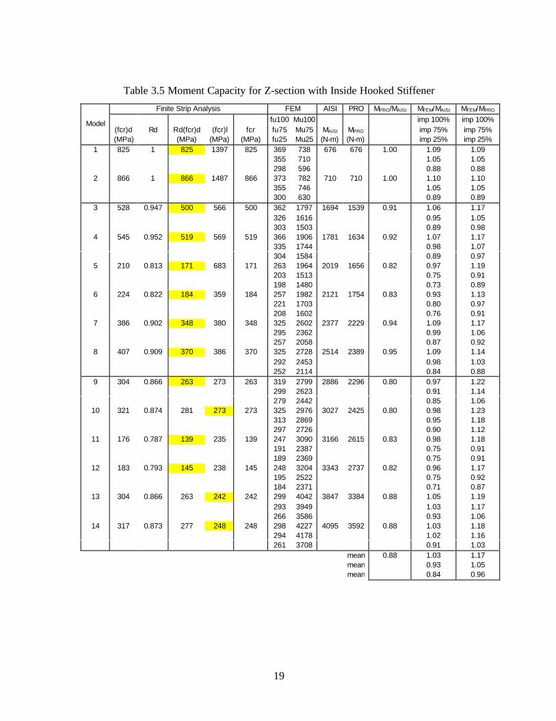
Table 3.5 Moment Capacity for Z-section with Inside Hooked Stiffener .........................19
Table 3.6 Moment Capacity for Z-section with Outside Hooked Stiffener.......................20
Table 3.7 Finite Element Results for Imperfection Magnitude 100% Probability of
Exceedance.................................................................................................................21
Table 3.8 Finite Element Results for Imperfection Magnitude 75% Probability of
Exceedance.................................................................................................................21
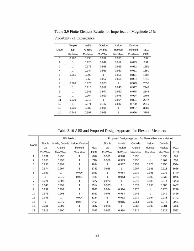
Table 3.9 Finite Element Results for Imperfection Magnitude 25% Probability of
Exceedance.................................................................................................................22
Table 3.10 AISI Method and Proposed Design Approach for Flexural Members Method
Results........................................................................................................................22
Table 3.11 Summary of Models Geometry........................................................................26
Table 3.12 Moment Capacity for Z-section 12ZS3.25 with Sloping Lip, Simple Lip,
Outside Angled, Inside Angled Stiffeners .................................................................27
Table 3.13 Finite Element Results for Imperfection Magnitude 100% Probability of
Exceedance.................................................................................................................28
Table 3.14 Finite Element Results for Imperfection Magnitude 75% Probability of
Exceedance.................................................................................................................29
Table 3.15 Finite Element Results for Imperfection Magnitude 25% Probability of
Exceedance.................................................................................................................29

Table 3.16 AISI Method and Proposed Design Approach for Flexural Members Method
Results........................................................................................................................29
Table 8.1 FEM Results Ultimate Compressive Strength vs. Imperfection Type 1 vs. Type
2 .................................................................................................................................59
LIST OF FIGURES
Figure 1.1 Isolated Flange-Stiffener Model.........................................................................3
Figure 1.2 Post-Buckling Capacity of Edge Stiffened Flanges ...........................................4
Figure 1.3 Imperfection Sensitivity of Edge Stiffened Flanges...........................................4
Figure 2.1 Isolated Flange-Complex Stiffener Model (a) Inside Angled Stiffener (b)
Outside Angled Stiffener (c) Inside Hooked Stiffener (d) Outside Hooked Stiffener.6
Figure 2.2 Boundary and Loading Condition......................................................................7
Figure 2.3 (a) Local Buckling (b) Distortional Buckling (c) Geometric Imperfection.......7
Figure 2.4 Post-Buckling Capacity of Inside Angled Stiffener ...........................................8
Figure 2.5 Imperfection Sensitivity of Inside Angled Stiffener ..........................................8
Figure 2.6 Post-Buckling Capacity of Outside Angled Stiffener ........................................9
Figure 2.7 Imperfection Sensitivity of Outside Angled Stiffener........................................9
Figure 2.8 Post-Buckling Capacity of Inside Hooked Stiffener ........................................10
Figure 2.9 Imperfection Sensitivity of Inside Hooked Stiffener........................................10
Figure 2.10 Post-Buckling Capacity of Outside Hooked Stiffener....................................11
Figure 2.11 Imperfection Sensitivity of Outside Hooked Stiffener...................................11
Figure 3.1 Z-section with (a) Simple Lip Stiffener (b) Inside Angled Stiffener (c) Outside
Angled Stiffener (d) Inside Hooked Stiffener (e) Outside Hooked Stiffener ............14
Figure 3.2 (a) Boundary and Loading Condition (b) Local Buckling (c) Distortional
Buckling (d) Initial Geometric Imperfection.............................................................15
Figure 3.3 Post-Buckling Capacity by Finite Element Method.........................................23
Figure 3.4 Post-Buckling Capacity by AISI Method.........................................................23
Figure 3.5 Post-Buckling Capacity by Proposed Design Approach for Flexural Members
...................................................................................................................................24

Figure 3.6 Z-section 12ZS3.25 with (a) Sloping Lip Stiffener 50 degree respect to the
flange (b) Simple Lip Stiffener (c) Outside Angled Stiffener (d) Inside Angled
Stiffener......................................................................................................................25
Figure 3.7 Boundary and Loading Condition....................................................................26
Figure 3.8 Post-Buckling Capacity by Finite Element Method.........................................30
Figure 3.9 Post-Buckling Capacity by AISI Method.........................................................30
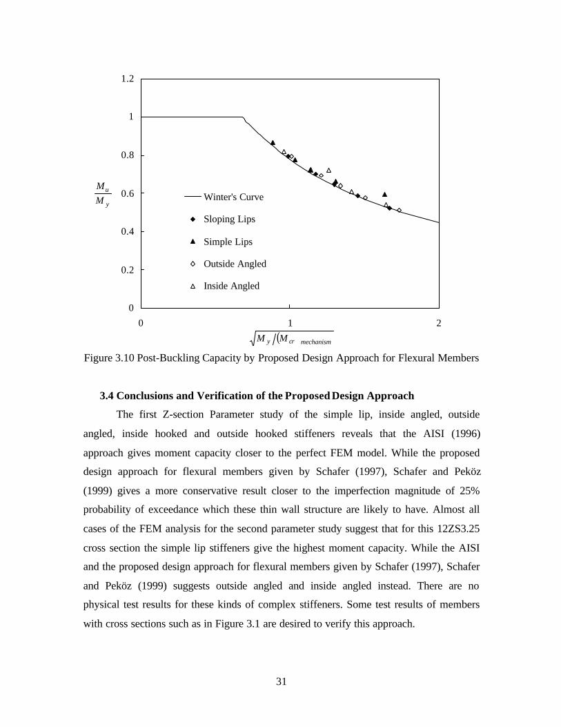
Figure 3.10 Post-Buckling Capacity by Proposed Design Approach for Flexural Members
...................................................................................................................................31
Figure 4.1 Post-Buckling Capacity by Finite Element Method (same as figure 3.3) ........33
Figure 4.2 Post-Buckling Capacity by Proposed Method with (Rd)a - data ......................33
Figure 4.3 Reduction Factor for Distortional Buckling Rd vs. (Rd)a..................................34
Figure 4.4 Post-Buckling Capacity by Proposed Method with (Rd)a.................................34
Figure 4.5 Post-Buckling Capacity by Proposed Method with (Rd)b - data ......................35
Figure 4.6 Reduction Factor for Distortional Buckling Rd vs. (Rd)b..................................35
Figure 4.7 Post-Buckling Capacity by Proposed Method with (Rd)b.................................36
Figure 5.1 12ZS3.25x090 with (a) Sloping Lip Stiffener 50 degree respect to the flange
(b) Simple Lip Stiffener (c) Outside Angled Stiffener (d) Inside Angled Stiffener .37
Figure 5.2 Flanges Width Optimization (a) AISI Method (b) Proposed Method.............37
Figure 5.3 12ZS3.25x090 with (a) Sloping Lip Stiffener 50 degree respect to the flange
(b) Simple Lip Stiffener (c) Outside Angled Stiffener (d) Inside Angled Stiffener .38
Figure 5.4 Stiffeners Length Optimization (a) AISI Method (b) Proposed Method ........38
Figure 5.5 12ZS3.25x090 with (a) Sloping Lip Stiffener 50 degree respect to the flange
(b) Simple Lip Stiffener (c) Outside Angled Stiffener (d) Inside Angled Stiffener .39
Figure 5.6 Stiffener/Flange Ratio Optimization (a) AISI Method (b) Proposed Method.39
Figure 6.1 Various Types of Stiffener in Consideration…………………………………42
Figure 6.2 Boundary and Loading Condition……………………………………………42
Figure 6.3 Inside Angled Optimization by Finite Element Method……………………..43
Figure 6.4 Outside Angled Optimization by Finite Element Method…………………... 44
Figure 6.5 Inside and Outside Angled Optimization by AISI Method…………………. 45
Figure 6.6 Inside Angled Optimization by Proposed Method…………………………...46
Figure 6.7 Outside Angled Optimization by Proposed Method…………………………47

Figure 7.1 Details of Arrangement of Experiment, Rinchen (1998) .................................48
Figure 7.2 Simulation of Experimental Arrangement........................................................49
Figure 7.3 Failure Mode of DHS200-1.8 with Experimental Arrangement ......................49
Figure 7.4 Finite Element Results for DHS200-1.8 with Experiment Arrangement .........50
Figure 8.1 (a) Cross-section Geometry (b) Geometric Imperfection (c) Boundary
Condition and Geometric Imperfection.....................................................................52
Figure 8.2 Imperfection Signal along the Length of the Member .....................................53
Figure 8.3 One-sided Power Spectral Density...................................................................54
Figure 8.4 Band-Limited White Noise: (a) Correlation Function (b) One-sided Spectral
Density, G(ω).............................................................................................................55
Figure 8.5 Zero mean, σi =1.0 Stationary Guassian Stochastic Process: 1 Signal.............56
Figure 8.6 Zero mean, σi =1.0 Stationary Guassian Stochastic Process: 10 Signal...........57
Figure 8.7 Ultimate Compressive Strength vs. Standard Deviation of the Imperfection
Signal..........................................................................................................................57
Figure 8.8 Histograms and Normal Distributions Density Function for each σimp,i..........58
Figure 8.9 Eigenmodes (a) Local Buckling Imperfection Type 1, d1 (b) Distortional
Buckling Imperfection Type 2, d2 .............................................................................59
Figure 8.10 Ultimate Compressive Strength vs. Imperfection Type 1 vs. Type 2 ............60
Figure 8.11 Initial Geometric Imperfection by Stochastic Process vs. Eigenmodes .........60
1
A Design Approach for Complex Stiffeners
1 Introduction
This report presents a design approach for laterally braced cold-formed steel
flexural members with edge stiffened flanges other than simple lips. The objectives of
the research are as follows:
− To study the feasibility of using the design method for flexural members given by
Schafer (1997), Schafer and Peköz (1999) to design these complex stiffeners and then
compare the results with the finite element method and AISI (1996). (Chapters 2-4)
− To use a computer program, CU-EWA, developed to perform parameter studies for
cross section optimization. (Chapter 5-6)
− To conduct a preliminary study on a two-point bending experiment setup as
preparation for future testing by doing a full finite element simulation of the
experimental arrangement and by making comparisons with previous physical test
results. (Chapter 7)
− To study an alternative approach for introducing the initial geometric imperfection by
using the stochastic process to randomly generate signals for the imperfection
geometric shape instead of introducing the initial geometric imperfection by
superimposing the eigenmodes. (Chapter 8)
The following is a summary of the design procedures for flexural members given
by Schafer (1997), Schafer and Peköz (1999). The design procedures are based on the
need for the integration of the distortional mode into the design procedure. Two
behavioral phenomena must be considered. First, the distortional mode has less post-
buckling capacity than the local mode. Second, the distortional mode has the ability to
control failure even when it occurs at a higher critical stress than the local mode. A
design method incorporating these phenomena is needed to provide an integrated
approach to strength prediction involving local and distortional buckling. For consistency
with the existing cold-form steel design specifications an effective width approach was
undertaken. Effective section properties are based on effective widths, b.

2
wb ρ= (1)
where w is the actual element width and post-buckling reduction factor, ρ , is
( )ρ λ λ= −1 0 22. for λ > 0.673 otherwise ρ = 1. (2)
where
cry ff=λ (3)
In order to properly integrate distortional buckling, reduced post-buckling
capacity in the distortional mode and the ability of the distortional mode to control the
failure mechanism even when at a higher buckling stress than the local mode must be
incorporated. Therefore, the critical buckling stress of the element was defined by
comparing the local buckling stress and distortional buckling stress to determine the
governing mode as follows:
( ) ( ) ( )[ ]f f R fcr cr local d cr dist= min ,
. (4)
Rdd
=+
+
min ,
..1
1171
0 3λ
where ( )λd y cr distf f=
. (5)
Rd reflects the reduced strength in mechanisms associated with distortional
failures. For Rd < 1 this method provides an additional reduction on the post-buckling
capacity. Further, the method allows the distortional mode to control situations where the
distortional buckling stress is greater than the local buckling stress. Thus, Rd provides a
framework for solving the problem of predicting the failure mode and reducing the post-
buckling capacity in the distortional mode. Schafer (1997), Schafer and Peköz (1999)
developed the expression for Rd based on post-buckling capacity as shown in Figure 1.2,
1.3 and from the experimental results of Hancock et al. (1994). With fcr of the element
known the effective width of each element may readily be determined and the effective
section properties generated.
To investigate the post-buckling behavior and develop the expression for Rd the
authors analyzed an isolated flange-stiffener model as shown in Figure 1.1 rather then
using the full section. Two types of imperfections, local and distortional mode, are
superposed to give the initial geometric imperfections. The magnitude of the imperfection
is selected based on the statistical summary provided in Schafer (1997), Schafer and
Peköz (1999). Then the ultimate strength of these isolated flanges is found for different

3
magnitudes of imperfection. Two maximum imperfection magnitudes, one at 25% and
the other at 75% probability of exceedance, are used. The percent differences in the
strength are used to measure the imperfection sensitivity.
( ) ( )( ) ( )( ) %100
.%25.%7521
.%25.%75 ×+
−
impuimpu
impuimpu
ff
ff (6)
The error bars in Figure 1.2 show the range of strengths predicted for
imperfections varying over the central 50% portion of expected imperfection magnitudes.
The greater the error bars, the greater the imperfection sensitivity. A contour plot of this
imperfection sensitivity statistic is shown in Figure 1.3. Stocky members tending to
failure in the distortional mode have the highest sensitivity.
The design approach given by Schafer (1997), Schafer and Peköz (1999) was
developed based on simple lips edge stiffeners. Therefore, before adopting this approach
for other types of stiffeners verification on the reduction factor for distortional stress, Rd
is needed. This is done by creating a post-buckling capacity graph and imperfection
sensitivity contour plot on the types of stiffeners in interest for comparison with the
original Figure 1.2 and 1.3. In this research 4 types of complex stiffeners shown in Figure
2.1 are studied.
b
dθ
c.
s.c.
Figure 1.1 Isolated Flange-Stiffener Model

4
0
0.2
0.4
0.6
0.8
1
0 1 2 3
Winter's CurveLocal Buckling FailuresDistortional Buckling Failures
error bars indicate the range of strengths observed between imperfection magnitudes of 25 and 75 % probability of exceedance
P
( )f fy cr mechanism
ff
u
y
Figure 1.2 Post-Buckling Capacity of Edge Stiffened Flanges
( )( )
f
fcr local
cr dist.
( )f fy cr mechanism
0 0.5 1 1.5 2 2.50
0.2
0.4
0.6
0.8
1
1.2
1.4
1.6
1.8
2
15%
15%
10%
10%
5%
5%
0%
HIGH
MEDIUM
LOW
MEDIUM
Figure 1.3 Imperfection Sensitivity of Edge Stiffened Flanges

5
2 Design Approach for Complex Stiffeners
Similar to the design approach given by Schafer (1997), Schafer and Peköz
(1999) to account for the distortional buckling an evaluation of the reduction factor for
distortional stress, Rd based on experimental and FEM studies must be considered. FEM
studies were carried out for 4 types of complex stiffeners shown in Figure 2.1.
2.1 Finite Element Study
In order to study the post-buckling behavior of complex stiffened elements
nonlinear FEM analyses are performed using ABAQUS. To study only the complex
stiffened element behavior an idealization of the boundary conditions at the web/flange
junction are made by restraining all degrees of freedom except for the translation along
the length. Roller supports are used at both ends. To avoid localized failure at the ends,
the uniform load has been distributed to the first row of elements. Boundary conditions
are shown in Figure 2.2. The material model used is elastic-plastic with strain hardening
and fy = 347 MPa. Residual stress is also included with a 30% yield stress throughout the
thickness in the longitudinal direction. The residual stresses are assumed tension on the
outside and compression in the inside of the section.
Initial geometric imperfection is introduced by superimposing the eigenmodes for
the local and distortional buckling shown in Figure 2.3. The magnitude of the
imperfection is selected based on the statistical summary provided in Schafer (1997),
Schafer and Peköz (1999). Four types of complex stiffeners shown in Figure 2.1 have
been studied. The length of the model is selected by using the length that would give the
least buckling strength in the distortional mode, which is obtained, by using the Finite
Strip Method CUFSM. Table 2.1 summarizes the geometry of the members. An
imperfection sensitivity study has been performed for each type of stiffener. Figure 2.4,
2.6, 2.8, 2.10 and contour plot in Figure 2.5, 2.7, 2.9, 2.11 show the results. For each type
of stiffener a total of 42 models were investigated.

6
B
d
a
B
d a
B
d
B
d
(a)
(d)
(b)
(c) 2a 2
a
2a2
a
Figure 2.1 Isolated Flange-Complex Stiffener Model (a) Inside Angled Stiffener
(b) Outside Angled Stiffener (c) Inside Hooked Stiffener (d) Outside Hooked
Stiffener
Table 2.1 Geometry of Members *
B d a
25 6.25 0,3.125,6.25
12.5 0,6.25,12.5
50 6.25 0,3.125,6.25
12.5 0,6.25,12.5
25 0,12.5,25
75 6.25 0,3.125,6.25
12.5 0,6.25,12.5
25 0,12.5,25
37.5 0,18.75,37.5
100 6.25 0,3.125,6.25
12.5 0,6.25,12.5
25 0,12.5,25
37.5 0,18.75,37.5
50 0,25,50
* Thickness = 1 mm in all cases

7
1
5
4
3
2
6 Roller Support
DOF 2,3 restrained
Roller Support DOF 2,3 restrained
Fixed, DOF 2-6 restrained
ABAQUS S9R5 Shell Element
DOF
Figure 2.2 Boundary and Loading Condition
(a)
(b)
(c)
Figure 2.3 (a) Local Buckling (b) Distortional Buckling (c) Geometric Imperfection

8
error bars indicate the range of strenghtsobserved between imperfection magnitudes of25 and 75 % probability of exceedance
0
0.2
0.4
0.6
0.8
1
1.2
0 1 2 3
Winter's Curve
Distortional Buckling Failure
Local Buckling Failure
Figure 2.4 Post-Buckling Capacity of Inside Angled Stiffener
Figure 2.5 Imperfection Sensitivity of Inside Angled Stiffener
( )mechanismcry ff
( )( ) .distcr
localcr
f
f
y
u
ff
( )mechanismcry ff

9
error bars indicate the range of strenghtsobserved between imperfection magnitudes of25 and 75 % probability of exceedance
0
0.2
0.4
0.6
0.8
1
1.2
0 1 2 3
Winter's Curve
Distortional Buckling Failure
Local Buckling Failure
Figure 2.6 Post-Buckling Capacity of Outside Angled Stiffener
Figure 2.7 Imperfection Sensitivity of Outside Angled Stiffener
( )( ) .distcr
localcr
f
f
( )mechanismcry ff
y
u
ff
( )mechanismcry ff

10
error bars indicate the range of strenghtsobserved between imperfection magnitudes of25 and 75 % probability of exceedance
0
0.2
0.4
0.6
0.8
1
1.2
0 1 2 3
Winter's Curve
Distortional Buckling Failure
Local Buckling Failure
Figure 2.8 Post-Buckling Capacity of Inside Hooked Stiffener
Figure 2.9 Imperfection Sensitivity of Inside Hooked Stiffener
y
u
ff
( )mechanismcry ff
( )mechanismcry ff
( )( ) .distcr
localcr
f
f

11
error bars indicate the range of strenghtsobserved between imperfection magnitudes of25 and 75 % probability of exceedance
0
0.2
0.4
0.6
0.8
1
1.2
0 1 2 3
Winter's Curve
Distortional Buckling Failure
Local Buckling Failure
Figure 2.10 Post-Buckling Capacity of Outside Hooked Stiffener
Figure 2.11 Imperfection Sensitivity of Outside Hooked Stiffener
( )( ) .distcr
localcr
f
f
( )mechanismcry ff
y
u
ff
( )mechanismcry ff

12
2.2 Conclusion and Verification of the Proposed Design Approach
It can be seen that the imperfection sensitivity contour plots are similar to those
obtained by edge stiffened flanges. Therefore, the reduction factor for distortional stress,
Rd is expected to be similar to Schafer (1997), Schafer and Peköz (1999).
3 Parametric Studies on Laterally Braced Flexural Members with Complex
Stiffeners
Two Z-section parameter studies are carried out for different types of stiffeners to
compare the moment capacity determined by FEM, AISI (1996) approach and the
proposed design approach for flexural members given by Schafer (1997), Schafer and
Peköz (1999). First parameter study consists of different Z-section geometries with all
cross sections having the same thickness while the second parameter study uses one
standard Z-section but varies thickness. The cross sections selected for both these
parameter studies are intend to cover a wide range of slendernesses and maintain the
cross section area between each types of stiffeners to compare the efficiency.
3.1 Z-Section Parameter Study for Constant Thickness
The parameter study is done by changing different widths of the web, flange and
stiffeners for five types of stiffeners simple lip, inside angled, outside angled, inside
hooked, and outside hooked stiffeners. All cross sections have the same thickness. Figure
3.1 and Table 3.1 summarize the geometry of the members. Local and distortional
buckling stresses obtained by finite strip method are used for the proposed design
approach for flexural members given by Schafer (1997), Schafer and Peköz (1999).
Results for each type of stiffeners for this parameter study are shown in Table 3.2, 3.3,
3.4, 3.5, and 3.6. Table 3.7, 3.8, 3.9,3.10 and Figure 3.3, 3.4, 3.5 summarize the results
for different approaches.
13
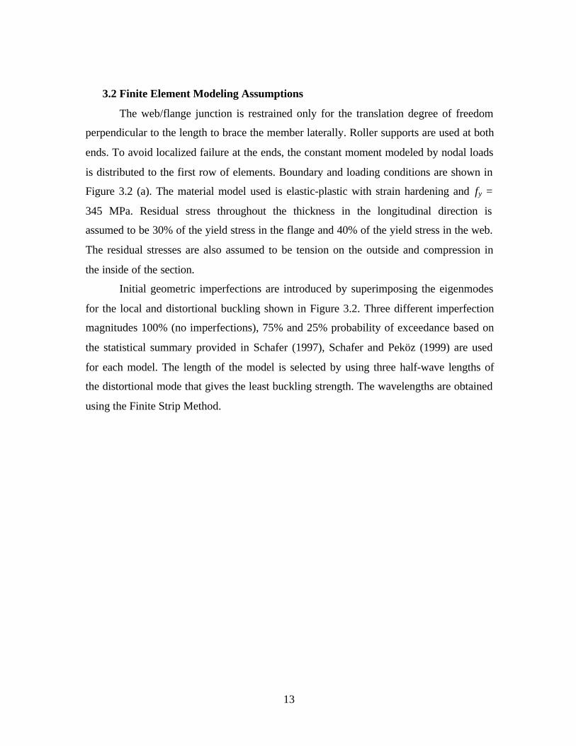
3.2 Finite Element Modeling Assumptions
The web/flange junction is restrained only for the translation degree of freedom
perpendicular to the length to brace the member laterally. Roller supports are used at both
ends. To avoid localized failure at the ends, the constant moment modeled by nodal loads
is distributed to the first row of elements. Boundary and loading conditions are shown in
Figure 3.2 (a). The material model used is elastic-plastic with strain hardening and fy =
345 MPa. Residual stress throughout the thickness in the longitudinal direction is
assumed to be 30% of the yield stress in the flange and 40% of the yield stress in the web.
The residual stresses are also assumed to be tension on the outside and compression in
the inside of the section.
Initial geometric imperfections are introduced by superimposing the eigenmodes
for the local and distortional buckling shown in Figure 3.2. Three different imperfection
magnitudes 100% (no imperfections), 75% and 25% probability of exceedance based on
the statistical summary provided in Schafer (1997), Schafer and Peköz (1999) are used
for each model. The length of the model is selected by using three half-wave lengths of
the distortional mode that gives the least buckling strength. The wavelengths are obtained
using the Finite Strip Method.

14
Figure 3.1 Z-section with (a) Simple Lip Stiffener (b) Inside Angled Stiffener (c) Outside
Angled Stiffener (d) Inside Hooked Stiffener (e) Outside Hooked Stiffener
Table 3.1 Summary of Models Geometry *
Dimensions
Length, L (mm)
H B d a Simple Inside Outside Inside OutsideModel
(mm) (mm) (mm) (mm) Lip Angled Angled Hooked Hooked
1 50 25 6.25 3.125 630 600 570 600 570
2 50 25 6.25 6.25 780 690 570 630 570
3 100 25 6.25 3.125 720 690 660 660 630
4 100 25 6.25 6.25 900 780 660 720 660
5 100 50 6.25 3.125 1170 1080 1050 1050 1050
6 100 50 6.25 6.25 1410 1200 1110 1140 1080
7 100 50 12.5 6.25 1830 1740 1620 1680 1620
8 100 50 12.5 12.5 2190 1950 1650 1830 1650
9 150 25 6.25 3.125 720 660 660 660 630
10 150 25 6.25 6.25 930 780 690 750 690
11 150 50 6.25 3.125 1230 1170 1140 1140 1110
12 150 50 6.25 6.25 1500 1290 1200 1230 1170
13 150 50 12.5 6.25 1980 1860 1770 1800 1740
14 150 50 12.5 12.5 2370 2100 1800 1980 1770
* Thickness = 1 mm in all cases
B
d + aa
H
d + a
B
B
d
H
d
B
a
a
B
d
H
d
B
a
B
d
H
d
B
B
d
H
d
B
2a
2a
2a
2a
(a) (b)
(c) (d) (e)
2a
2a
2a 2
a

15
Figure 3.2 (a) Boundary and Loading Condition (b) Local Buckling (c) Distortional
Buckling (d) Initial Geometric Imperfection
Lateral Bracing
Roller Support
Roller Support
(a)
(b)
(c)
(d)
L

16
Table 3.2 Moment Capacity for Z-section with Simple Lip Stiffener
Finite Strip Analysis FEM AISI PRO MPRO/MAISI MFEM/MAISI MFEM/MPRO
fu100 Mu100 imp 100% imp 100%(fcr)d Rd Rd(fcr)d (fcr)l fcr fu75 Mu75 MAISI MPRO imp 75% imp 75%
Model
(MPa) (MPa) (MPa) (MPa) fu25 Mu25 (N-m) (N-m) imp 25% imp 25%1 942 1 942 1346 942 376 745 670 670 1.00 1.11 1.11
362 718 1.07 1.07309 613 0.92 0.92
2 1132 1 1132 1263 1132 380 771 682 687 1.01 1.13 1.12373 757 1.11 1.10340 691 1.01 1.01
3 583 0.961 560 573 560 373 1840 1687 1574 0.93 1.09 1.17337 1665 0.99 1.06314 1551 0.92 0.99
4 659 0.979 645 573 573 380 1947 1734 1645 0.95 1.12 1.18355 1823 1.05 1.11322 1650 0.95 1.00
5 245 0.835 205 345 205 265 1969 1945 1740 0.89 1.01 1.13226 1684 0.87 0.97222 1650 0.85 0.95
6 317 0.873 277 348 277 309 2356 2185 1976 0.90 1.08 1.19285 2174 1.00 1.10242 1845 0.84 0.93
7 445 0.922 410 342 342 314 2489 2190 2201 1.01 1.14 1.13289 2292 1.05 1.04252 1994 0.91 0.91
8 542 0.951 515 317 317 307 2492 2120 2226 1.05 1.18 1.12299 2430 1.15 1.09276 2243 1.06 1.01
9 331 0.879 291 266 266 324 2828 2879 2282 0.79 0.98 1.24311 2719 0.94 1.19291 2544 0.88 1.12
10 380 0.899 341 266 266 330 2998 2950 2372 0.80 1.02 1.26321 2916 0.99 1.23308 2794 0.95 1.18
11 204 0.808 165 238 165 252 3149 3010 2742 0.91 1.05 1.15221 2766 0.92 1.01218 2719 0.90 0.99
12 255 0.841 215 238 215 252 3227 3468 3081 0.89 0.93 1.05246 3160 0.91 1.03219 2815 0.81 0.91
13 342 0.884 302 238 238 293 3930 3465 3345 0.97 1.13 1.17278 3736 1.08 1.12250 3356 0.97 1.00
14 400 0.907 363 235 235 278 3857 3321 3466 1.04 1.16 1.11271 3766 1.13 1.09253 3508 1.06 1.01
mean 0.94 1.08 1.15mean 1.02 1.09mean 0.93 0.99
(fcr)d – Distortional Buckling critical stressRd – Reduction factor for Distortional Buckling critical stress(fcr)l – Local Buckling critical stressfcr – Controlling critical stressfu100, fu75, fu25 – Ultimate stress for imperfection magnitudes 100%, 75% and 25% probability of exceedanceMu100, Mu75, Mu25 – Ultimate moment for imperfection magnitudes 100%, 75% and 25% probability of exceedanceM FEM, M AISI, M PRO – Nominal Moment from FEM, AISI and proposed design approach for flexural members

17
Table 3.3 Moment Capacity for Z-section with Inside Angled Stiffener
Finite Strip Analysis FEM AISI PRO MPRO/MAISI MFEM/MAISI MFEM/MPRO
fu Mu imp 100% imp 100%(fcr)d Rd Rd(fcr)d (fcr)l fcr fu25 Mu25 MAISI MPRO imp 75% imp 75%
Model
(MPa) (MPa) (MPa) (MPa) fu75 Mu75 (N-m) (N-m) imp 25% imp 25%1 869 1.000 869 1418 869 373 744 675 675 1.00 1.10 1.10
355 709 1.05 1.05299 596 0.88 0.88
2 980 1.000 980 1504 980 373 776 705 705 1.00 1.10 1.10362 755 1.07 1.07305 635 0.90 0.90
3 549 0.953 522 566 522 362 1795 1693 1554 0.92 1.06 1.16332 1647 0.97 1.06306 1517 0.90 0.98
4 600 0.966 580 569 569 369 1918 1775 1666 0.94 1.08 1.15337 1753 0.99 1.05300 1558 0.88 0.94
5 221 0.820 181 342 181 264 1968 2027 1678 0.83 0.97 1.17209 1556 0.77 0.93206 1536 0.76 0.92
6 245 0.835 205 355 205 274 2105 2131 1805 0.85 0.99 1.17238 1832 0.86 1.02204 1569 0.74 0.87
7 407 0.909 370 386 370 315 2517 2372 2263 0.95 1.06 1.11296 2360 0.99 1.04251 2002 0.84 0.88
8 466 0.929 433 390 390 308 2570 2490 2407 0.97 1.03 1.07296 2470 0.99 1.03247 2059 0.83 0.86
9 311 0.870 270 262 262 320 2800 2885 2283 0.79 0.97 1.23296 2595 0.90 1.14275 2404 0.83 1.05
10 345 0.885 305 262 262 325 2977 3020 2384 0.79 0.99 1.25312 2850 0.94 1.20294 2693 0.89 1.13
11 183 0.793 145 235 145 252 3145 3184 2638 0.83 0.99 1.19217 2709 0.85 1.03215 2688 0.84 1.02
12 200 0.806 161 238 161 236 3044 3365 2819 0.84 0.90 1.08207 2666 0.79 0.95190 2452 0.73 0.87
13 317 0.873 277 245 245 301 4056 3842 3386 0.88 1.06 1.20286 3856 1.00 1.14261 3521 0.92 1.04
14 359 0.891 320 248 248 302 4261 4052 3569 0.88 1.05 1.19292 4130 1.02 1.16262 3696 0.91 1.04
mean 0.89 1.03 1.15mean 0.94 1.06mean 0.85 0.95

18
Table 3.4 Moment Capacity for Z-section with Outside Angled Stiffener
Finite Strip Analysis FEM AISI PRO MPRO/MAISI MFEM/MAISI MFEM/MPRO
fu100 Mu100 imp 100% imp 100%(fcr)d Rd Rd(fcr)d (fcr)l fcr fu75 Mu75 MAISI MPRO imp 75% imp 75%
Model
(MPa) (MPa) (MPa) (MPa) fu25 Mu25 (N-m) (N-m) imp 25% imp 25%1 749 0.997 746 1521 746 369 737 675 673 1.00 1.09 1.09
352 702 1.04 1.04298 594 0.88 0.88
2 645 0.976 630 1542 630 369 769 705 678 0.96 1.09 1.13355 740 1.05 1.09314 654 0.93 0.96
3 486 0.935 455 573 455 362 1795 1693 1499 0.89 1.06 1.20345 1708 1.01 1.14309 1532 0.90 1.02
4 428 0.916 392 580 392 366 1900 1775 1510 0.85 1.07 1.26339 1764 0.99 1.17305 1583 0.89 1.05
5 207 0.811 168 400 168 267 1991 2027 1635 0.81 0.98 1.22258 1922 0.95 1.18229 1708 0.84 1.04
6 204 0.808 165 393 165 275 2113 2131 1675 0.79 0.99 1.26262 2015 0.95 1.20232 1784 0.84 1.07
7 348 0.887 309 393 309 318 2536 2372 2145 0.90 1.07 1.18297 2371 1.00 1.11252 2008 0.85 0.94
8 297 0.863 256 393 256 317 2639 2490 2116 0.85 1.06 1.25292 2435 0.98 1.15247 2056 0.83 0.97
9 286 0.858 246 266 246 317 2779 2885 2239 0.78 0.96 1.24297 2604 0.90 1.16284 2486 0.86 1.11
10 269 0.849 228 266 228 318 2913 3020 2285 0.76 0.96 1.27295 2702 0.89 1.18278 2544 0.84 1.11
11 173 0.785 135 242 135 252 3154 3184 2576 0.81 0.99 1.22249 3115 0.98 1.21236 2947 0.93 1.14
12 169 0.782 132 245 132 252 3244 3365 2631 0.78 0.96 1.23190 2448 0.73 0.93172 2216 0.66 0.84
13 273 0.851 232 248 232 299 4032 3842 3327 0.87 1.05 1.21280 3777 0.98 1.14265 3567 0.93 1.07
14 235 0.829 194 248 194 294 4159 4052 3292 0.81 1.03 1.26280 3964 0.98 1.20254 3588 0.89 1.09
mean 0.85 1.03 1.22mean 0.96 1.14mean 0.86 1.02
19
Table 3.5 Moment Capacity for Z-section with Inside Hooked Stiffener
Finite Strip Analysis FEM AISI PRO MPRO/MAISI MFEM/MAISI MFEM/MPRO
fu100 Mu100 imp 100% imp 100%(fcr)d Rd Rd(fcr)d (fcr)l fcr fu75 Mu75 MAISI MPRO imp 75% imp 75%
Model
(MPa) (MPa) (MPa) (MPa) fu25 Mu25 (N-m) (N-m) imp 25% imp 25%1 825 1 825 1397 825 369 738 676 676 1.00 1.09 1.09
355 710 1.05 1.05298 596 0.88 0.88
2 866 1 866 1487 866 373 782 710 710 1.00 1.10 1.10355 746 1.05 1.05300 630 0.89 0.89
3 528 0.947 500 566 500 362 1797 1694 1539 0.91 1.06 1.17326 1616 0.95 1.05303 1503 0.89 0.98
4 545 0.952 519 569 519 366 1906 1781 1634 0.92 1.07 1.17335 1744 0.98 1.07304 1584 0.89 0.97
5 210 0.813 171 683 171 263 1964 2019 1656 0.82 0.97 1.19203 1513 0.75 0.91198 1480 0.73 0.89
6 224 0.822 184 359 184 257 1982 2121 1754 0.83 0.93 1.13221 1703 0.80 0.97208 1602 0.76 0.91
7 386 0.902 348 380 348 325 2602 2377 2229 0.94 1.09 1.17295 2362 0.99 1.06257 2058 0.87 0.92
8 407 0.909 370 386 370 325 2728 2514 2389 0.95 1.09 1.14292 2453 0.98 1.03252 2114 0.84 0.88
9 304 0.866 263 273 263 319 2799 2886 2296 0.80 0.97 1.22299 2623 0.91 1.14279 2442 0.85 1.06
10 321 0.874 281 273 273 325 2976 3027 2425 0.80 0.98 1.23313 2869 0.95 1.18297 2726 0.90 1.12
11 176 0.787 139 235 139 247 3090 3166 2615 0.83 0.98 1.18191 2387 0.75 0.91189 2369 0.75 0.91
12 183 0.793 145 238 145 248 3204 3343 2737 0.82 0.96 1.17195 2522 0.75 0.92184 2371 0.71 0.87
13 304 0.866 263 242 242 299 4042 3847 3384 0.88 1.05 1.19293 3949 1.03 1.17266 3586 0.93 1.06
14 317 0.873 277 248 248 298 4227 4095 3592 0.88 1.03 1.18294 4178 1.02 1.16261 3708 0.91 1.03
mean 0.88 1.03 1.17mean 0.93 1.05mean 0.84 0.96

20
Table 3.6 Moment Capacity for Z-section with Outside Hooked Stiffener
Finite Strip Analysis FEM AISI PRO MPRO/MAISI MFEM/MAISI MFEM/MPRO
fu100 Mu100 imp 100% imp 100%(fcr)d Rd Rd(fcr)d (fcr)l fcr fu75 Mu75 MAISI MPRO imp 75% imp 75%
Model
(MPa) (MPa) (MPa) (MPa) fu25 Mu25 (N-m) (N-m) imp 25% imp 25%1 735 0.994 731 1490 731 369 738 676 671 0.99 1.09 1.10
355 710 1.05 1.06319 637 0.94 0.95
2 642 0.975 626 1532 626 366 768 710 683 0.96 1.08 1.12345 724 1.02 1.06294 617 0.87 0.90
3 480 0.933 447 573 447 359 1780 1694 1496 0.88 1.05 1.19331 1643 0.97 1.10307 1523 0.90 1.02
4 428 0.916 392 576 392 362 1888 1781 1518 0.85 1.06 1.24321 1674 0.94 1.10295 1536 0.86 1.01
5 200 0.806 161 359 161 266 1982 2019 1623 0.80 0.98 1.22201 1498 0.74 0.92199 1488 0.74 0.92
6 193 0.801 155 386 155 271 2089 2121 1652 0.78 0.98 1.26223 1722 0.81 1.04216 1668 0.79 1.01
7 342 0.884 302 386 302 317 2535 2377 2137 0.90 1.07 1.19296 2364 0.99 1.11250 2003 0.84 0.94
8 297 0.863 256 393 256 323 2711 2514 2134 0.85 1.08 1.27290 2433 0.97 1.14248 2080 0.83 0.97
9 283 0.856 242 262 242 321 2814 2886 2241 0.78 0.97 1.26302 2644 0.92 1.18284 2487 0.86 1.11
10 269 0.849 228 266 228 316 2894 3027 2300 0.76 0.96 1.26298 2736 0.90 1.19282 2581 0.85 1.12
11 169 0.782 132 238 132 246 3082 3166 2573 0.81 0.97 1.20194 2430 0.77 0.94189 2361 0.75 0.92
12 162 0.776 126 242 126 247 3191 3343 2607 0.78 0.95 1.22179 2308 0.69 0.89174 2251 0.67 0.86
13 269 0.849 228 245 228 298 4023 3847 3323 0.86 1.05 1.21292 3939 1.02 1.19262 3539 0.92 1.06
14 235 0.829 194 248 194 294 4169 4095 3315 0.81 1.02 1.26285 4041 0.99 1.22250 3547 0.87 1.07
mean 0.84 1.02 1.21mean 0.91 1.08mean 0.83 0.99

21
Table 3.7 Finite Element Results for Imperfection Magnitude 100%
Probability of Exceedance
Simple Inside Outside Inside Outside
Model Lip Angled Angled Hooked Hooked MMAX
MSL/MMAX MIA/MMAX MOA/MMAX MIH/MMAX MOH/MMAX (N-m)
1 1 0.998 0.989 0.990 0.990 745
2 0.986 0.993 0.984 1 0.981 782
3 1 0.976 0.976 0.976 0.967 1840
4 1 0.985 0.976 0.979 0.970 1947
5 0.989 0.988 1 0.986 0.995 1991
6 1 0.894 0.897 0.841 0.887 2356
7 0.957 0.967 0.975 1 0.975 2602
8 0.913 0.942 0.967 1 0.994 2728
9 1 0.990 0.983 0.990 0.995 2828
10 1 0.993 0.972 0.993 0.965 2998
11 0.999 0.997 1 0.980 0.977 3154
12 0.995 0.938 1 0.988 0.984 3244
13 0.969 1 0.994 0.997 0.992 4056
14 0.905 1 0.976 0.992 0.978 4261
MSL, MIA, MOA, MIH, MOH – Z-section moment capacity for Simple Lip,
Inside Angled, Outside Angled, Inside Hooked and Outside Hooked stiffeners
MMAX – Maximum moment capacity between MSL, MIA, MOA, MIH, MOH
Table 3.8 Finite Element Results for Imperfection Magnitude 75%
Probability of Exceedance
Simple Inside Outside Inside Outside
Model Lip Angled Angled Hooked Hooked MMAX
MSL/MMAX MIA/MMAX MOA/MMAX MIH/MMAX MOH/MMAX (N-m)
1 1 0.988 0.978 0.990 0.990 718
2 1 0.997 0.978 0.985 0.957 757
3 0.975 0.964 1 0.946 0.962 1708
4 1 0.962 0.967 0.957 0.918 1823
5 0.876 0.810 1 0.788 0.780 1922
6 1 0.842 0.927 0.783 0.792 2174
7 0.967 0.995 1 0.996 0.997 2371
8 0.984 1 0.986 0.993 0.985 2470
9 1 0.954 0.958 0.965 0.973 2719
10 1 0.977 0.926 0.984 0.938 2916
11 0.888 0.870 1 0.766 0.780 3115
12 1 0.843 0.774 0.798 0.730 3160
13 0.946 0.976 0.956 1 0.998 3949
14 0.901 0.988 0.949 1 0.967 4178
22
Table 3.9 Finite Element Results for Imperfection Magnitude 25%
Probability of Exceedance
Simple Inside Outside Inside Outside
Model Lip Angled Angled Hooked Hooked MMAX
MSL/MMAX MIA/MMAX MOA/MMAX MIH/MMAX MOH/MMAX (N-m)
1 0.962 0.936 0.932 0.935 1 637
2 1 0.920 0.947 0.912 0.893 691
3 1 0.978 0.988 0.969 0.982 1551
4 1 0.944 0.959 0.960 0.931 1650
5 0.966 0.899 1 0.866 0.871 1708
6 1 0.850 0.967 0.868 0.904 1845
7 0.969 0.973 0.975 1 0.973 2058
8 1 0.918 0.917 0.943 0.927 2243
9 1 0.945 0.977 0.960 0.978 2544
10 1 0.964 0.910 0.976 0.924 2794
11 0.923 0.912 1 0.804 0.801 2947
12 1 0.871 0.787 0.842 0.799 2815
13 0.936 0.982 0.995 1 0.987 3586
14 0.946 0.997 0.968 1 0.956 3708
Table 3.10 AISI and Proposed Design Approach for Flexural Members
AISI Method Proposed Design Approach for Flexural Members Method
Simple Inside, Outside Inside, Outside Simple Inside Outside Inside Outside
Lip Angled Hooked MMAX Lip Angled Angled Hooked Hooked MMAX
Model
MSL/MMAX MIOA/MMAX MIOH/MMAX (N-m) MSL/MMAX MIA/MMAX MOA/MMAX MIH/MMAX MOH/MMAX (N-m)
1 0.991 0.998 1 676 0.991 0.998 0.996 1 0.993 676
2 0.960 0.993 1 710 0.968 0.993 0.956 1 0.962 710
3 0.996 0.999 1 1694 1 0.987 0.952 0.978 0.950 1574
4 0.974 0.997 1 1781 0.988 1 0.907 0.981 0.911 1666
5 0.959 1 0.996 2027 1 0.964 0.939 0.951 0.932 1740
6 1 0.975 0.971 2185 1 0.913 0.848 0.888 0.836 1976
7 0.921 0.998 1 2377 0.973 1 0.948 0.985 0.944 2263
8 0.843 0.991 1 2514 0.925 1 0.879 0.993 0.886 2407
9 0.997 0.999 1 2886 0.994 0.994 0.975 1 0.976 2296
10 0.975 0.998 1 3027 0.978 0.983 0.942 1 0.949 2425
11 0.946 1 0.994 3184 1 0.962 0.939 0.954 0.938 2742
12 1 0.970 0.964 3468 1 0.915 0.854 0.888 0.846 3081
13 0.901 0.999 1 3847 0.988 1 0.982 0.999 0.981 3386
14 0.811 0.990 1 4095 0.965 0.994 0.916 1 0.923 3592

23
0
0.2
0.4
0.6
0.8
1
1.2
0 1 2
Winter's Curve
Simple Lips
Inside Angled
Outside Angled
Inside Hooked
Outside Hookederror bars indicate the range of strenghtsobserved between imperfection magnitudes of25 and 75 % probability of exceedance
Figure 3.3 Post-Buckling Capacity by Finite Element Method
0
0.2
0.4
0.6
0.8
1
1.2
0 1 2
Winter's Curve
Simple Lips
Inside Angled
Outside Angled
Inside Hooked
Outside Hooked
Figure 3.4 Post-Buckling Capacity by AISI Method
y
u
MM
( )mechanismcry MM
y
u
MM
( )mechanismcry MM

24
0
0.2
0.4
0.6
0.8
1
1.2
0 1 2
Winter's Curve
Simple Lips
Inside Angled
Outside Angled
Inside Hooked
Outside Hooked
Figure 3.5 Post-Buckling Capacity by Proposed Design Approach for Flexural Members
y
u
MM
( )mechanismcry MM

25
3.3 Z-Section Parameter Study for Various Thickness
This second parameter study was carried out by modifying the stiffeners of a
standard cross section 12ZS3.25, which has a sloping lip stiffener. The sloping lip
stiffener was modified into simple lip, outside angled and inside angled stiffeners. Cross-
section area for each type of stiffeners is maintained to compare the efficiency. This was
done for different thickness. The finite element assumptions are the same as in the first
parameter study except for the yield stress and the lateral bracing conditions. This study
uses a 55 ksi yield stress and instead of fully bracing along the length as in the first
parameter study, only four brace points are used. Brace points one at each end and
additional ones at one-third of the length, which is the same length as the half-wave
lengths of the distortional mode that gives the least buckling strength. Figure 3.7 shows
the second parameter study boundary and loading conditions. For this cross section and
bracing length, full formation of the distortional mode is still possible without causing a
lateral-torsional failure. Figure 3.6 and Table 3.11 summarize the geometry of the
members. Results for each type of stiffeners for this parameter study are shown in Table
3.12. Table 3.13, 3.14, 3.15, 3.16 and Figure 3.8, 3.9, 3.10 summarizes the results for
different approaches.
Figure 3.6 Z-section 12ZS3.25 with (a) Sloping Lip Stiffener 50 degree respect to the
flange (b) Simple Lip Stiffener (c) Outside Angled Stiffener (d) Inside Angled Stiffener
B d
H
dB
Bd
H
d
B
B
H
B
B
H
B
2d
2d
2d
2d
2d 2
d
2d
2d
(a) (b) (d)(c)

26
Table 3.11 Summary of Models Geometry
Dimensions
Length, L (in.)
H B d t Sloping Simple Inside OutsideModel
(in.) (in.) (in.) (in.) Lip Lip Angled Angled
1 12 3.25 0.75 0.135 54 60 51 51
2 12 3.25 0.75 0.105 63 69 57 60
3 12 3.25 0.75 0.090 69 75 63 754 12 3.25 0.75 0.075 75 84 69 72
5 12 3.25 0.75 0.060 84 96 78 81
Figure 3.7 Boundary and Loading Condition
Roller SupportLateral Bracing
Roller Support
3L
3L
3L

27
Table 3.12 Moment Capacity for Z-section 12ZS3.25 with Sloping Lip, Simple Lip,
Outside Angled, Inside Angled Stiffeners
Finite Strip Analysis FEM AISI PRO MPRO/MAISI MFEM/MAISI MFEM/MPRO
fu100 Mu100 imp 100% imp 100%(fcr)d Rd Rd(fcr)d (fcr)l fcr fu75 Mu75 MAISI MPRO imp 75% imp 75%
Model
(ksi) (ksi) (ksi) (ksi) fu25 Mu25 (kip-in.) (kip-in.) imp 25% imp 25%1 56 0.888 50 77 50 51 468 463 397 0.86 1.01 1.18
48 436 0.94 1.1041 378 0.82 0.95
2 40 0.838 33 59 33 45 322 327 275 0.84 0.98 1.1736 262 0.80 0.9537 267 0.82 0.97
3 33 0.809 26 46 26 41 253 263 219 0.83 0.96 1.1531 194 0.74 0.8930 185 0.70 0.84
4 26 0.776 20 32 20 36 188 192 167 0.87 0.98 1.1327 141 0.73 0.8426 135 0.70 0.81
5 20 0.738 15 21 15 28 118 134 119 0.89 0.88 0.9923 94 0.71 0.79
Slo
ping
Lip
Stif
fene
r
22 91 0.68 0.761 71 0.922 65 102 65 54 488 473 426 0.90 1.03 1.14
48 433 0.92 1.0245 411 0.87 0.96
2 51 0.875 45 63 45 48 338 339 302 0.89 1.00 1.1240 283 0.83 0.9437 264 0.78 0.88
3 43 0.847 36 46 36 44 268 276 242 0.88 0.97 1.1136 221 0.80 0.9135 214 0.78 0.88
4 34 0.816 28 32 28 35 180 204 186 0.91 0.88 0.9633 170 0.83 0.9134 174 0.86 0.94
5 26 0.779 21 21 21 29 120 145 135 0.93 0.83 0.8929 122 0.84 0.90
Sim
ple
Lip
Stif
fene
r
28 118 0.81 0.871 54 0.881 47 69 47 50 454 480 393 0.82 0.95 1.16
46 420 0.88 1.0741 376 0.78 0.96
2 38 0.830 31 54 31 43 305 345 271 0.79 0.89 1.1336 257 0.74 0.9537 264 0.77 0.97
3 31 0.800 24 46 24 39 239 286 215 0.75 0.84 1.1131 192 0.67 0.8931 188 0.66 0.87
4 24 0.766 19 32 19 34 176 208 163 0.78 0.84 1.0827 141 0.67 0.8626 135 0.65 0.82
5 18 0.728 13 21 13 27 114 144 116 0.81 0.79 0.9823 97 0.68 0.84
Out
side
Ang
led
Stif
fene
r
23 95 0.66 0.81

28
1 59 0.896 53 77 53 51 466 480 406 0.85 0.97 1.1546 420 0.88 1.0441 368 0.77 0.91
2 42 0.846 36 58 36 45 318 345 283 0.82 0.92 1.1338 269 0.78 0.9538 270 0.78 0.96
3 34 0.817 28 45 28 41 255 286 244 0.85 0.89 1.0435 213 0.74 0.8734 207 0.72 0.85
4 27 0.784 22 31 22 35 182 208 172 0.83 0.87 1.0629 149 0.72 0.8728 145 0.70 0.84
5 21 0.746 16 20 16 28 117 144 123 0.85 0.82 0.9527 112 0.78 0.91
Insi
de A
ngle
d S
tiffe
ner
24 100 0.69 0.81mean 0.85 0.93 1.09mean 0.79 0.93mean 0.76 0.89
Table 3.13 Finite Element Results for Imperfection Magnitude 100%
Probability of Exceedance
Sloping Simple Outside Inside
Model Lip Lip Angled Angled MMAX
MSLL/MMAX MSL/MMAX MIA/MMAX MOA/MMAX (kip-in.)
1 0.960 1 0.930 0.955 488
2 0.950 1 0.902 0.941 338
3 0.941 1 0.892 0.949 268
4 1 0.954 0.935 0.970 188
5 0.983 1 0.946 0.977 120
MSLL, MSL, MIA, MOA – Z-section moment capacity for Sloping Lip, Simple Lip,
Inside Angled, Outside Angled stiffeners
MMAX – Maximum moment capacity between MSLL, MSL, MIA, MOA

29
Table 3.14 Finite Element Results for Imperfection Magnitude 75%
Probability of Exceedance
Sloping Simple Outside Inside
Model Lip Lip Angled Angled MMAX
MSLL/MMAX MSL/MMAX MIA/MMAX MOA/MMAX (kip-in.)
1 1 0.995 0.965 0.965 436
2 0.925 1 0.908 0.952 283
3 0.878 1 0.867 0.962 221
4 0.828 1 0.828 0.880 170
5 0.774 1 0.801 0.919 122
Table 3.15 Finite Element Results for Imperfection Magnitude 25%
Probability of Exceedance
Sloping Simple Outside Inside
Model Lip Lip Angled Angled MMAX
MSLL/MMAX MSL/MMAX MIA/MMAX MOA/MMAX (kip-in.)
1 0.920 1 0.915 0.895 411
2 0.987 0.976 0.975 1 270
3 0.864 1 0.878 0.965 214
4 0.772 1 0.772 0.831 174
5 0.770 1 0.805 0.850 118
Table 3.16 AISI and Proposed Design Approach for Flexural Members
AISI Method Proposed Design Approach for Flexural Members Method
Sloping Simple Outside, Inside Sloping Simple Outside Inside
Lip Lip Angled MMAX Lip Lip Angled Angled MMAX
Model
MSLL/MMAX MSL/MMAX MIOA/MMAX (kip-in.) MSLL/MMAX MSL/MMAX MIA/MMAX MOA/MMAX (kip-in.)
1 0.964 0.986 1 480 0.931 1 0.921 0.951 426
2 0.948 0.983 1 345 0.913 1 0.899 0.938 302
3 0.919 0.963 1 286 0.898 0.993 0.882 1 244
4 0.921 0.978 1 208 0.895 1 0.876 0.923 186
5 0.924 1 0.996 145 0.885 1 0.863 0.914 135

30
error bars indicate the range of strenghtsobserved between imperfection magnitudes of25 and 75 % probability of exceedance
0
0.2
0.4
0.6
0.8
1
1.2
0 1 2
Winter's Curve
Sloping Lips
Simple Lips
Outside Angled
Inside Angled
Figure 3.8 Post-Buckling Capacity by Finite Element Method
0
0.2
0.4
0.6
0.8
1
1.2
0 1 2
Winter's Curve
Sloping Lips
Simple Lips
Outside Angled
Inside Angled
Figure 3.9 Post-Buckling Capacity by AISI Method
y
u
MM
( )mechanismcry MM
y
u
MM
( )mechanismcry MM
31
0
0.2
0.4
0.6
0.8
1
1.2
0 1 2
Winter's Curve
Sloping Lips
Simple Lips
Outside Angled
Inside Angled
Figure 3.10 Post-Buckling Capacity by Proposed Design Approach for Flexural Members
3.4 Conclusions and Verification of the Proposed Design Approach
The first Z-section Parameter study of the simple lip, inside angled, outside
angled, inside hooked and outside hooked stiffeners reveals that the AISI (1996)
approach gives moment capacity closer to the perfect FEM model. While the proposed
design approach for flexural members given by Schafer (1997), Schafer and Peköz
(1999) gives a more conservative result closer to the imperfection magnitude of 25%
probability of exceedance which these thin wall structure are likely to have. Almost all
cases of the FEM analysis for the second parameter study suggest that for this 12ZS3.25
cross section the simple lip stiffeners give the highest moment capacity. While the AISI
and the proposed design approach for flexural members given by Schafer (1997), Schafer
and Peköz (1999) suggests outside angled and inside angled instead. There are no
physical test results for these kinds of complex stiffeners. Some test results of members
with cross sections such as in Figure 3.1 are desired to verify this approach.
y
u
MM
( )mechanismcry MM

32
4 Verification of the Reduction Factor for Distortional Buckling, Rd
Schafer (1997), Schafer and Peköz (1999) developed the expression for Rd based
on post-buckling capacity as shown in Figure 1.2, 1.3 and from the experimental results
of Hancock et al. (1994). Based on the FEM results in the previous study section 3.1,
two alternative Rd expressions are developed here (Rd)a and (Rd)b. The alternative
expressions are then compared with the original Rd.
By combining the FEM results of different types of stiffeners from Figure 3.3 a
regression line may be obtained as in Figure 4.1. A new expression for (Rd)a can be found
by letting Rd be a variable and recalculating back to find the best (Rd)a that fits the FEM
regression line from the proposed design approach for flexural members given by Schafer
(1997), Schafer and Peköz (1999). The result of this attempt is shown in Figure 4.2. As
seen the data points do not all match the regression line due to the condition that (Rd)a is
to be only equal to or less then one. These new Rd values result from all models which are
(Rd)a - data in Figure 4.3 are the data points of the new expression (Rd)a. The same
approach is also used to develop (Rd)b but instead of trying to match the FEM regression
line as (Rd)a the expression for (Rd)b is found based on trying to match each model to its
own FEM result. Results of this are shown in Figure 4.5 and 4.6.
The original Rd is also plotted in Figure 4.3 and 4.6 to compare with (Rd)a and
(Rd)b. As seen (Rd)a is very close to Rd but (Rd)b gives a larger reduction factor then Rd.
Figures 4.4 and 4.7 show the results from using the two new expressions in the proposed
design approach for flexural members given by Schafer (1997), Schafer and Peköz
(1999). Comparing these figures with Figure 3.5 one can see that they do not differ much,
thus verifying that the original Rd used in the previous study is suitable for the overall
cross sections in this study.

33
y = -0.4911x2 + 0.5085x + 0.8368
0
0.2
0.4
0.6
0.8
1
1.2
0 1 2
Figure 4.1 Post-Buckling Capacity by Finite Element Method (same as figure 3.3)
0
0.2
0.4
0.6
0.8
1
1.2
0 1 2
Proposed Method Matching FEM line
Figure 4.2 Post-Buckling Capacity by Proposed Method with (Rd)a - data
y
u
MM
( )mechanismcry MM
( ) ( ) 8368.05085.04911.0 ++
−=
mechanismcr
y
mechanismcr
y
y
u
M
M
M
M
MM
y
u
MM
( )mechanismcry MM

34
0
0.2
0.4
0.6
0.8
1
1.2
0 1 2
Rd(Rd)a - data(Rd)a
Figure 4.3 Reduction Factor for Distortional Buckling Rd vs. (Rd)a
0
0.2
0.4
0.6
0.8
1
1.2
0 1 2
Winter's Curve
Proposed Method with (Rd)a
Figure 4.4 Post-Buckling Capacity by Proposed Method with (Rd)a
y
u
MM
( )mechanismcry MM
( ) dad
.e.R λ−= 3369025516730.d <λwhere
dR
( ) .distcryd ff=λ

35
0
0.2
0.4
0.6
0.8
1
1.2
0 1 2
FEM Method
Proposed Method Matching FEM data
Figure 4.5 Post-Buckling Capacity by Proposed Method with (Rd)b - data
0
0.2
0.4
0.6
0.8
1
1.2
0 1 2
Rd(Rd)b - data(Rd)b
Figure 4.6 Reduction Factor for Distortional Buckling Rd vs. (Rd)b
y
u
MM
( )mechanismcry MM
dR
( ) .distcryd ff=λ
( ) dbd
.e.R λ−= 507040616730.d <λwhere

36
0
0.2
0.4
0.6
0.8
1
1.2
0 1 2
Winter's Curve
Proposed Method with (Rd)b
Figure 4.7 Post-Buckling Capacity by Proposed Method with (Rd)b
5 Cross Section Optimization Study I
A computer program CU-EWA was developed to compute the nominal flexural
strength, Mn, and the nominal axial strength, Pn, using two approaches. These
approaches are the AISI (1996) method of initial yielding and the proposed design
approach for flexural members given by Schafer (1997), Schafer and Peköz (1999). This
program, CU-EWA, is used here to perform parameter studies on the cross section
optimization. The nominal flexural strength divided by the cross section area is used here
as the cross section efficiency index where three parameters are investigated
independently: flange width, stiffener length and stiffener/flange ratio. For each
parameter study four different types of stiffeners are considered to compare their
advantages. Results from two approaches, the AISI (1996) initial yielding method and the
proposed design approach for flexural members given by Schafer (1997), Schafer and
Peköz (1999) are also compared. For the proposed method the local and distortional
buckling stresses are required. Therefore, a finite strip analysis, CUFSM, was preformed
for each cross section first. This parameter study was carried out for a standard cross
section 12ZS3.25x090 with modified lips as in Figure 3.6.
y
u
MM
( )mechanismcry MM

37
5.1 Parameter Study I – Flanges Width Optimization
For the four types of stiffeners the flange width is varied to find the cross section
that gives the highest efficiency index, Mn/A. Figure 5.1 shows how the geometry
changes as the flange width increases and Figure 5.2 shows the results from this
parameter study. The vertical line at flange width 3.25 in. is for the original cross section
dimensions. Results from the proposed method in this parameter study suggest that by
changing the stiffeners to simple lip and decreasing the flange width from the original
values the cross section efficiency may be increased.
Figure 5.1 12ZS3.25x090 with (a) Sloping Lip Stiffener 50 degree respect to the flange
(b) Simple Lip Stiffener (c) Outside Angled Stiffener (d) Inside Angled Stiffener
Figure 5.2 Flanges Width Optimization (a) AISI Method (b) Proposed Method
(a)
(c)
(b)
(d)

38
5.2 Parameter Study II – Stiffeners Length Optimization
Considering the stiffener length to be a varied variable and all others dimensions
to be constant an optimum stiffener length may be found for different types of stiffeners.
Figure 5.3 shows how the geometry changes as the stiffener length increases and Figure
5.4 shows the results from this parameter study. The vertical line at stiffener length 0.75
in. is the original cross section value. Results from the proposed method in this parameter
study suggest that a simple lip with a length of 1 in. is the best section considering cross
section efficiency.
Figure 5.3 12ZS3.25x090 with (a) Sloping Lip Stiffener 50 degree respect to the flange
(b) Simple Lip Stiffener (c) Outside Angled Stiffener (d) Inside Angled Stiffener
Figure 5.4 Stiffeners Length Optimization (a) AISI Method (b) Proposed Method
(a)
(c)
(b)
(d)

39
5.3 Parameter Study III – Stiffener/Flange Ratio Optimization
By changing both the stiffener and flange lengths but still maintaining the cross
section area, the best stiffener/flange ratio may be found. Figure 5.5 shows how the
geometry changes as the stiffener/flange ratio increases and Figure 5.6 shows the results
from this parameter study. The first stiffener/flange ratio, 0.23, is the original cross
section value. Results from the proposed method suggest that a simple lip with a
stiffener/flange ratio of 0.33 is the best section considering efficiency.
Figure 5.5 12ZS3.25x090 with (a) Sloping Lip Stiffener 50 degree respect to the flange
(b) Simple Lip Stiffener (c) Outside Angled Stiffener (d) Inside Angled Stiffener
Figure 5.6 Stiffener/Flange Ratio Optimization (a) AISI Method (b) Proposed Method
(a)
(c)
(b)
(d)

40
6 Cross Section Optimization Study II
This second cross section optimization study was carried out by modifying the
stiffeners of a standard cross section 9CS3x060, which has a simple lip stiffener. The
simple lip stiffener was modified into different types of inside angled and outside angled
stiffeners as shown in Figure 6.1. The nominal flexural strength divided by the cross
section area is used here as the cross section efficiency index where the total length of the
stiffener, d is increased to find the optimal section. Three different approaches to
calculate the section capacity, the FEM, AISI (1996) initial yielding method and the
proposed design approach for flexural members given by Schafer (1997), Schafer and
Peköz (1999) are compared. Results from these different approaches are shown in Figure
6.3, 6.4, 6.5, 6.6 and 6.7.
6.1 Finite Element Modeling Assumptions
In this study the length of the member is taken as the half-wave lengths of the
distortional mode that gives the least buckling strength. Lateral bracings are only
provided by roller supports at the ends. For this cross section and member length, full
formation of the distortional mode is still possible without causing a lateral-torsional
failure. To avoid localized failure at the ends, the constant moment modeled by nodal
loads is distributed into the first two rows of elements. Boundary and loading conditions
are shown in Figure 6.2. The material model used is elastic-plastic with strain hardening
and fy = 65 ksi. Residual stress throughout the thickness in the longitudinal direction is
assumed to be 25% of the yield stress in the flange, 40% of the yield stress in the web and
30% at of the yield stress in the corners. The residual stresses are also assumed to be
tension on the outside and compression in the inside of the section. Initial geometric
imperfections are introduced by superimposing the eigenmodes for the local and
distortional buckling. The imperfection magnitude 50% probability of exceedance based
on the statistical summary provided in Schafer (1997), Schafer and Peköz (1999) is used.

41
6.2 Conclusion
All three approaches agree well for the simple lip case that an optimized section
may be obtained by increasing the stiffener length from the original given length of d =
0.5 in. to about d = 1 in. The current AISI (1996) method does not distinguish between
the inside and outside angle stiffener. Results also show that this method is
unconservative compared with the other two approaches. The overall trend of the results
between the FEM and the proposed method shows agreement; that is, it is more efficient
to have inside angled stiffeners then simple lip or outside angled stiffeners. A wider range
of scattered data is obtained from thee FEM due to the initial geometric imperfection. A
study on sections with higher material yield stress has also been considered. Results are
similar to those obtained here where the inside angled stiffeners has slight advantage over
the simple lip and outside angled stiffeners

42
Figure 6.1 Various Types of Stiffener Under Consideration
Figure 6.2 Boundary and Loading Condition
(a)
(b) (c) (d) (e)
(f) (g) (h) (i)
Simple Lip Stiffener
Inside Angled Stiffener
Outside Angled Stiffener
Roller Support
Roller Support
M
M
L
ABAQUS S4R Shell Element

43
60
65
70
75
80
85
90
95
100
105
110
115
120
125
130
135
140
0 0.5 1 1.5 2 2.5 3
Stiffener Type (a)
Stiffener Type (b)
Stiffener Type (c)
Stiffener Type (d)
Stiffener Type (e)
Figure 6.3 Inside Angled Optimization by Finite Element Method
a
b
c
d
e
d, in.
AM u , kips/in.

44
45
50
55
60
65
70
75
80
85
90
95
100
105
110
115
120
125
130
135
140
0 0.5 1 1.5 2 2.5 3
Stiffener Type (a)
Stiffener Type (f)
Stiffener Type (g)
Stiffener Type (h)
Stiffener Type (i)
Figure 6.4 Outside Angled Optimization by Finite Element Method
a
d, in.
AM u , kips/in.
f
g
h
i

45
110
115
120
125
130
135
140
145
150
155
160
0 0.5 1 1.5 2 2.5 3
Figure 6.5 Inside and Outside Angled Optimization by AISI Method
a
(b, f)(c, g)
(d, h)(e, i)
d, in.
AM n , kips/in.

46
100
105
110
115
120
125
130
135
0 0.5 1 1.5 2 2.5 3
Figure 6.6 Inside Angled Optimization by Proposed Method
100
105
110
115
120
125
130
135
0 0.5 1 1.5 2 2.5 3
Figure 6.7 Outside Angled Optimization by Proposed Method
a
b
cd
e
af
g
h
i
d, in.
AM n , kips/in.
d, in.
AM n , kips/in.

47
7 An Experimental Study
The two-point bending test shown in Figure 7.1 performed by Rinchen (1998) is
studied here. A full finite element simulation of the experimental arrangement is carried
out to compare with the physical test results.
7.1 Finite Element Simulation of Experimental Arrangement
The two-point bending experiment setup shown in Figure 7.1 is simulated by
FEM. A pair of DHS200-1.8 sections is placed back-to-back with loading braces and end
support plates, which were modeled with a much thicker shell element compared to the
ones used for the DHS200-1.8 members and connected only at the bolts positions. Pins
and rollers were used at the end supports and concentrated loads. Residual stresses are
also introduced as in the previous study but no imperfections are incorporated in to the
analysis due to lack of actual imperfection measurement at the preliminary studies.
However, a first approximation can be obtained and results are expected to be reduced
when there are some imperfections. Figure 7.2 and 7.3 shows the model of this
simulation at the failure state.
7.2 Conclusion
As suggested by Rinchen (1998), due to the interaction of local buckling,
distortional buckling and shear at the loading points, tests resulted in providing section
strength for localized failure instead of providing the section strength for pure bending.
FEM simulation of the experiment arrangement with no imperfections incorporated
showed even lower moment capacity with the same local failure mode. Results are shown
and compared in Figure 7.4. Modification in the experimental arrangement is needed and
should be simulated by finite element before doing actual testing. Rinchen (1998) also
suggested some changes in the experimental set up.

48
Figure 7.1 Details of Arrangement of Experiment, Rinchen (1998)

49
Figure 7.2 Simulation of Experimental Arrangement
Figure 7.3 Failure Mode of DHS200-1.8 with Experimental Arrangement
Local Failure
Stress due to LoadingBrace Connections
1000 mm
1000 mm
1500 mm

50
0
2.5
5
7.5
10
12.5
15
17.5
0 5 10 15 20 25 30 35 40
Displacement, mm
Mom
ent,
kN-m
Figure 7.4 Finite Element Results for DHS200-1.8 with Experiment Arrangement
M=16.03
Displacment=37 mm
(Experimental test results gives M=17.5 kN-mDisplacement = 30.35 mm)

51
8 Initial Geometric Imperfection by Stochastic Process
The following is a joint study with Yongwook Kim in a structural reliability class.
One of the most important factors that affect on the compressive strength in thin-walled
sections such as cold-form steel is the geometric imperfection. In the previous study
initial geometric imperfection was introduced by superimposing the eigenmodes for the
local and distortional buckling. The magnitude of the imperfection was selected based on
the statistical summary provided in Schafer (1997), Schafer and Peköz (1999). An
alternative approach is studied here by using stochastic process to randomly generate
signals for the imperfection geometric shape. From large numbers of the simulations, the
relationships between ultimate compressive strength and standard deviation of the
imperfection signal can be obtained. But because of lack of imperfection measurements
there fore some assumptions had to be made first. The idea was to go threw the process
and understand the approach.
8.1 Definitions and Assumptions
8.1.1 Definitions of the Section
Rather then using a full cross section an isolated flange-stiffener model in uniform
compression is studied instead and a nonlinear FEM analyses are performed using
ABAQUS. To study only the simple lip stiffened element an idealization of the boundary
condition at the web/flange junction is made by restraining all degrees of freedom except
for the translation along the length. Roller supports are used at both ends and to avoid
localized failure at the ends the uniform load has been distributed to the first row of
elements. The Geometry and boundary conditions are shown in Figure 8.1. The material
model used is elastic-plastic with strain hardening and fy = 55 ksi. Residual stress is also
included with a 30% yield stress throughout the thickness in the longitudinal direction.
The residual stresses are assumed tension on the outside and compression in the inside of
the section. The length of the model is selected by using the length that would give the
least buckling strength in the distortional mode, which is obtained, by using the Finite
Strip Method CUFSM.

52
8.1.2 Definitions of the Imperfection
Only one type of imperfection shown in Figure 8.1 (b) is considered. The web to
flange junction is assumed to be perfectly straight while the web to stiffeners junction
will have longitudinal imperfection. The longitudinal imperfection signal is assumed to
be zero mean, real valued stationary Gaussian stochastic process for a certain standard
deviation because the imperfection is deviation from the perfect plane. Imperfection
between the web junction and stiffeners junction is assumed to be linear.
perfect geometry plane
- imperfection signal
linear assumption
load = fy
B = 1.625 in.
d = 0.5 in.
thickness = 0.057 in.
δ
assume linear
δ
(a) (b)
(c)
L = 33 in.
Figure 8.1 (a) Cross-section Geometry (b) Geometric Imperfection
(c) Boundary Condition and Geometric Imperfection

53
8.2 Probabilistic Model for Uncertain Parameters
8.2.1 Imperfection is zero mean stationary Gaussian stochastic process:
A stochastic process is a function of two variables the parameter t and the
probability parameter ω . X(t,ω) , t ∈ T , ω ∈ Ω where parameter t usually refers to time
but for geometric imperfection t will denote as location along the length of the member.
If a manufacturer makes the members in a same process and condition, a set of
imperfection data X(•,ω) of the members can be called as sample, sample path or
realization. In addition, X(•,ω) can also be called as a stationary stochastic process, since
due to uniformity of the manufacturing process, the distributions of X’s over the different
members (ω) for a fixed location ‘t’ should be the identical regardless of its location (t).
This is because if X(t)is finite dimensional distribution and it does not change at a time
shift for ∀n, ∀t1,…., ∀tn,
F(x1,x2,…,xn ; t1,t2,…,tn) = F(x1,x2,…,xn ; t1’,t2’,…,tn’)
then X(t) can be said to be stationary in the strict sense. That is, the distribution is only a
function of time lag (tk – tk’; k=1…n)
Imperfectionmagnitude: X(t) member 1
member 2
member n
.
.
.
Length of member
Figure 8.2 Imperfection Signal along the Length of the Member

54
8.2.2 Imperfection signal is assumed as:
t))(?sinWt)(?cos(Vs)t(X)t(X k
m
kkkkkm
~
∑=
+==1
If this process is zero mean, real valued, continuous, stationary Gaussian process then
]t)dV(? )(sint)dU(? )(cos[)t(X ω+ω= ∫∞
0 (*)
where U(ω) and V(ω) are real valued, zero mean, independent Gaussian process with
properties EdU2(ω)=EdV2(ω)=G(ω)dω. However, the measured imperfection data
cannot be continuous, the equation (*) cannot be obtained. Instead, discrete
approximation of this process is possible. If this process is assumed to be a discrete
version X(t) with one-sided truncated power. Then the stochastic process X(t) can be
approximated as
))tsin(W)tcos(V()t(X)t(X k
m
kkkkkm
~
ω+ωσ== ∑=1
where Vk and Wk are independent Gaussian random variables with zero means and unit
variances.
>
≤≤= ~
~
,0
0),()(ωω
ωωωω GG~
ωωωωσ ∆≅= ∫ )()(2
kIk GdG)(tG
~
ω1 ωk ωm Ik
~0 ~
ω
Figure 8.3 One-sided Power Spectral Density
spectral density,

55
8.2.3 Process is assumed as Band-Limited White Noise
If actual signals of imperfection from the measurement are available, the
correlation function from the definition may be obtained. However, since the data is not
available currently, the correlation function is assumed as Band-limited white noise,
which is shown in Figure 8.4. R(τ) = Gosin(ωcτ)/ τ. where ωc = 1.6 is selected from the
experimental result of Schafer (1997) from the Fourier Transform of some cold-form
steel members, truncation (ωc) is decided at the 1.6 rad/in frequency. Standard deviation
(σimp,i) of imperfection parameter is constant and decided from the assumptions that it
varies from 0.25 to 2.0 (0.25, 0.50, 0.75, 1.00, 1.25, 1.50, 1.75 and 2.00). These numbers
are normalized standard deviation by dividing actual standard deviation by thickness
0.057 in. Then square of one of the selected standard deviation (σimp,i) will be the total
area of the one-sided spectral density. That is, (σimp,i)2= Go,i x ωc where, i=1~8. Then Go
is obtained for each different σimp,i and fixed ωc. In addition, σk2 can be computed from
σk2 = (σimp,i)2/5. Finally, Vk,Wk will be randomly generated.
-6 -4 -2 0 2 4 6
-2
0
2
4
6
8
10
12
14x 10
-4
0 0.5 1 1.5 2 2.5 30
0.1
0.2
0.3
0.4
0.5
0.6
0.7
0.8
0.9
1x 10
-3
Go
ωc
discretization
(a) (b)
Figure 8.4 Band-Limited White Noise: (a) Correlation Function
(b) One-sided Spectral Density, G(ω)

56
8.2.4 Generation of Imperfection Signal
Total 30 numbers of signals were generated for each standard deviation. Figure
8.5 and 8.6 shows 1 and 10 numbers of signals generated when σi =1.0 (=0.057 in.). For
each standard deviation 30 numbers of signals were generated. Then with these, total 240
FEM analyses are implemented. Since 30 numbers of signals from one standard deviation
are completely different, the ultimate capacities show scatter. For each scatter, histogram
is made and relationships between ultimate compressive strength and standard deviation
of the imperfection signal can be obtained. Results are shown in Figure 8.7 and 8.8.
-0.25
-0.2
-0.15
-0.1
-0.05
0
0.05
0.1
0.15
0.2
0.25
0 11 22 33
Figure 8.5 Zero mean, σi =1.0 Stationary Guassian Stochastic Process: 1 Signal
δ, (in.)
Location along the length of the member, (in.)

57
-0.25
-0.2
-0.15
-0.1
-0.05
0
0.05
0.1
0.15
0.2
0.25
0 11 22 33
Figure 8.6 Zero mean, σi =1.0 Stationary Guassian Stochastic Process: 10 Signal
0.4
0.5
0.6
0.7
0.8
0.9
1
1.1
0 0.25 0.5 0.75 1 1.25 1.5 1.75 2 2.25
mean
Figure 8.7 Ultimate Compressive Strength vs. Standard Deviation of the Imperfection
Signal
Imperfection standard deviation, σimp
y
u
ff
Location along the length of the member, (in.)
δ, (in.)

58
0.6 0.8 10
5
10 N(0.89317,0.037224)
Histogram for Imperfection std. = 0.25
fu/fy0.6 0.8 1
0
5
10 N(0.84517,0.047276)
Histogram for Imperfection std. = 0.5
fu/fy
0.6 0.8 10
5
10 N(0.78083,0.071257)
Histogram for Imperfection std. = 0.75
fu/fy0.6 0.8 1
0
5
10 N(0.71083,0.052034)
Histogram for Imperfection std. = 1
fu/fy
0.6 0.8 10
5
10 N(0.70117,0.066875)
Histogram for Imperfection std. = 1.25
fu/fy0.4 0.6 0.8
0
5
10 N(0.66887,0.055825)
Histogram for Imperfection std. = 1.5
fu/fy
0.4 0.6 0.80
5
10 N(0.62293,0.051025)
Histogram for Imperfection std. = 1.75
fu/fy0.4 0.6 0.8
0
5
10 N(0.60793,0.07475)
Histogram for Imperfection std. = 2
fu/fy
Figure 8.8 Histograms and Normal Distributions Density Function for each σimp,i
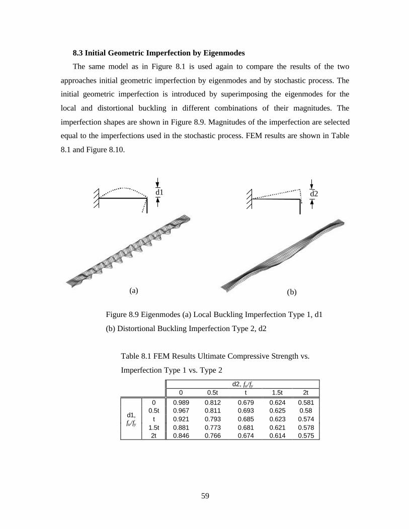
59
8.3 Initial Geometric Imperfection by Eigenmodes
The same model as in Figure 8.1 is used again to compare the results of the two
approaches initial geometric imperfection by eigenmodes and by stochastic process. The
initial geometric imperfection is introduced by superimposing the eigenmodes for the
local and distortional buckling in different combinations of their magnitudes. The
imperfection shapes are shown in Figure 8.9. Magnitudes of the imperfection are selected
equal to the imperfections used in the stochastic process. FEM results are shown in Table
8.1 and Figure 8.10.
(a) (b)
d2d1
Figure 8.9 Eigenmodes (a) Local Buckling Imperfection Type 1, d1
(b) Distortional Buckling Imperfection Type 2, d2
Table 8.1 FEM Results Ultimate Compressive Strength vs.
Imperfection Type 1 vs. Type 2
d2, fu/fy0 0.5t t 1.5t 2t
0 0.989 0.812 0.679 0.624 0.5810.5t 0.967 0.811 0.693 0.625 0.58
t 0.921 0.793 0.685 0.623 0.5741.5t 0.881 0.773 0.681 0.621 0.578
d1,fu/fy
2t 0.846 0.766 0.674 0.614 0.575

60
00.5t
t
1.5t
2t
00.5t
t
1.5t
2t
00.10.20.30.40.50.60.7
0.8
0.9
1
d2 d1
Figure 8.10 Ultimate Compressive Strength vs. Imperfection Type 1 vs. Type 2
0.4
0.5
0.6
0.7
0.8
0.9
1
1.1
0 0.25 0.5 0.75 1 1.25 1.5 1.75 2 2.25
Imperfection Type 1meanImperfection Type 2
Figure 8.11 Initial Geometric Imperfection by Stochastic Process vs. Eigenmodes
y
u
ff
y
u
ff
Imperfection standard deviation, σimp
61
8.4 Conclusion
Results from both approaches initial geometric imperfection by stochastic process
and by eigenmodes are compared in Figure 8.11. The imperfection type 1 and
imperfection type 2 lines are the results from introducing only their own imperfection
type which is the results from the first column and first row in Table 8.1 where theirs no
superimposing between the two modes. Results from the stochastic process and
imperfection type 2 line is surprisingly close and both have significant impact on the
strength reduction then the imperfection type 1. This shows that the section studied here
is more sensitive to fail in the distortional buckling then local buckling. Although there
were some assumptions made for the stochastic process but once some actual
measurement of the section in study is available developing a better mathematical model
is possible. The stochastic process used in this study is a 1 - dimensional stochastic
process. Further study in using a 2 - dimensional stochastic process that could simulate a
more realistic geometric imperfection plane is also of interest.
9 Summary and Conclusions
The approach formulated by Schafer (1997) also discussed in Schafer and Peköz
(1999) for simple lip stiffeners is also satisfactory for complex stiffeners. This conclusion
is based on finite element method studies. Finite element modeling agrees well with the
Australian test results but improvement in the experimental arrangement should be done
to avoid localize failure. Results from the cross section optimization study shows that it is
more efficient to have inside angled stiffener then simple lip or outside angled stiffener.

62
References
American Iron and Steel Institute, (1996). AISI Specification for the Design of Cold-
Formed Steel Structural Members. American Iron and Steel Institute Washington,
D.C.
Bernard, E.S., Bridge, R.S. and Hancock, G.J., (1996) “Design Methods for Profiled
Steel Decks with Intermediate Stiffeners,” Journal of Constructional Steel
Research, Vol.38, No.1, 1996, pp.61-88.
Hancock, G.J. and Kwon, Y.B., (1992). “Tests of Cold-Formed Channels with Local and
Distortional Buckling,” Journal of Structural Engineering, ASCE, Vol.117, No.7
July, 1992, pp. 1786-1803
H.O. Madsen, S. Krensky and N.C. Lind, (1986), Methods of Structural Safety, Prentice
Hall, Englewood Cliffs, NJ.
Jay L. Devore, (1991), Probability and Statistics for Engineering and the Science Third
Edition, Brooks/Cole Publishing Company, Pacific Grove, California.
J.R.Benjamin and C.A. Cornell, (1970), Probability, Statistics and Decision for Civil
Engineers, McGraw-Hill Hook Co., NY.
Mircea Grigoriu, (1995), Applied Non-Gaussian Processes, Examples, Theory,
Simulation, Linear Random Vibration, and MATLAB Solutions, PTR Prentice
Hall, Englewood Cliffs, NJ
Peköz, T., (1987). Development of a Unified Approach to the Design of Cold-Formed
Steel Members. American Iron and Steel Institute Research Report CF 87-1.
Rinchen, (1998). “Bending Section Strength of New Generation Cold-Formed Purlin
Shape” Bachelor of Engineering Thesis, School of Civil and Mining Engineering,
The University of Sydney

63
Schafer, B.W., (1997). “Cold-Formed Steel Behavior and Design: Analytical and
Numerical Modeling of Elements and Members with Longitudinal Stiffeners.”
Ph.D. Dissertation, Cornell University, Ithaca, New York
Schafer, B.W., Peköz, T.P., (1999). “Laterally Braced Cold-Formed Steel Flexural
Members with Edge Stiffened Flanges.” Journal of Structural Engineering,
125(2)
Standards Association of Australia, “Cold formed Steel Structures,” AS/NZS 4600-1996.
Schafer, B.W., “CUFSM, Cornell University Finite Strip Method User’s Manual v1.0d”
Cornell University, Ithaca, New York
T.T. Soong, Mircea Grigoriu, (1993), Random Vibration of Mechanical and Structural
Systems, PTR Prentice Hall, Englewood Cliffs, NJ.