Embed Size (px)
Citation preview

IBM®
DB2
Universal
Database™
Administration
Guide:
Planning
Version
8.2
SC09-4822-01
���


IBM®
DB2
Universal
Database™
Administration
Guide:
Planning
Version
8.2
SC09-4822-01
���

Before
using
this
information
and
the
product
it
supports,
be
sure
to
read
the
general
information
under
Notices.
This
document
contains
proprietary
information
of
IBM.
It
is
provided
under
a
license
agreement
and
is
protected
by
copyright
law.
The
information
contained
in
this
publication
does
not
include
any
product
warranties,
and
any
statements
provided
in
this
manual
should
not
be
interpreted
as
such.
You
can
order
IBM
publications
online
or
through
your
local
IBM
representative.
v
To
order
publications
online,
go
to
the
IBM
Publications
Center
at
www.ibm.com/shop/publications/order
v
To
find
your
local
IBM
representative,
go
to
the
IBM
Directory
of
Worldwide
Contacts
at
www.ibm.com/planetwide
To
order
DB2
publications
from
DB2
Marketing
and
Sales
in
the
United
States
or
Canada,
call
1-800-IBM-4YOU
(426-4968).
When
you
send
information
to
IBM,
you
grant
IBM
a
nonexclusive
right
to
use
or
distribute
the
information
in
any
way
it
believes
appropriate
without
incurring
any
obligation
to
you.
©
Copyright
International
Business
Machines
Corporation
1993
-
2004.
All
rights
reserved.
US
Government
Users
Restricted
Rights
–
Use,
duplication
or
disclosure
restricted
by
GSA
ADP
Schedule
Contract
with
IBM
Corp.

Contents
About
this
book
.
.
.
.
.
.
.
.
.
.
. vii
Who
should
use
this
book
.
.
.
.
.
.
.
.
. viii
How
this
book
is
structured
.
.
.
.
.
.
.
. viii
A
brief
overview
of
the
other
Administration
Guide
volumes
.
.
.
.
.
.
.
.
.
.
.
.
.
.
. ix
Administration
Guide:
Implementation
.
.
.
. ix
Administration
Guide:
Performance
.
.
.
.
. x
Part
1.
Database
concepts
.
.
.
.
.
. 1
Chapter
1.
Basic
relational
database
concepts
.
.
.
.
.
.
.
.
.
.
.
.
.
. 3
Database
objects
.
.
.
.
.
.
.
.
.
.
.
.
. 3
Configuration
parameters
.
.
.
.
.
.
.
.
.
. 11
Business
rules
for
data
.
.
.
.
.
.
.
.
.
.
. 12
Developing
a
backup
and
recovery
strategy
.
.
. 15
Automated
backup
operations
.
.
.
.
.
.
. 18
Automatic
maintenance
.
.
.
.
.
.
.
.
.
. 18
High
availability
disaster
recovery
(HADR)
feature
overview
.
.
.
.
.
.
.
.
.
.
.
.
.
.
. 23
Security
.
.
.
.
.
.
.
.
.
.
.
.
.
.
. 24
Authentication
.
.
.
.
.
.
.
.
.
.
.
.
. 25
Authorization
.
.
.
.
.
.
.
.
.
.
.
.
. 25
Units
of
work
.
.
.
.
.
.
.
.
.
.
.
.
. 26
Chapter
2.
Parallel
database
systems
29
Data
partitioning
.
.
.
.
.
.
.
.
.
.
.
. 29
Parallelism
.
.
.
.
.
.
.
.
.
.
.
.
.
. 30
Input/output
parallelism
.
.
.
.
.
.
.
.
. 30
Query
parallelism
.
.
.
.
.
.
.
.
.
.
. 30
Utility
parallelism
.
.
.
.
.
.
.
.
.
.
. 33
Partition
and
processor
environments
.
.
.
.
.
. 34
Single
partition
on
a
single
processor
.
.
.
.
. 34
Single
partition
with
multiple
processors
.
.
. 35
Multiple
partition
configurations
.
.
.
.
.
. 36
Summary
of
parallelism
best
suited
to
each
hardware
environment
.
.
.
.
.
.
.
.
. 40
Chapter
3.
About
data
warehousing
.
. 43
What
solutions
does
data
warehousing
provide?
.
. 43
Data
warehouse
objects
.
.
.
.
.
.
.
.
.
. 43
Subject
areas
.
.
.
.
.
.
.
.
.
.
.
.
. 44
Warehouse
sources
.
.
.
.
.
.
.
.
.
.
. 44
Warehouse
targets
.
.
.
.
.
.
.
.
.
.
. 44
Warehouse
control
databases
.
.
.
.
.
.
. 44
Warehouse
agents
and
agent
sites
.
.
.
.
.
. 44
Processes
and
steps
.
.
.
.
.
.
.
.
.
.
. 45
Warehouse
tasks
.
.
.
.
.
.
.
.
.
.
.
.
. 47
Part
2.
Database
design
.
.
.
.
.
. 49
Chapter
4.
Logical
database
design
.
. 51
What
to
record
in
a
database
.
.
.
.
.
.
.
. 51
Database
relationships
.
.
.
.
.
.
.
.
.
.
. 52
One-to-many
and
many-to-one
relationships
.
. 52
Many-to-many
relationships
.
.
.
.
.
.
.
. 53
One-to-one
relationships
.
.
.
.
.
.
.
.
. 53
Ensure
that
equal
values
represent
the
same
entity
.
.
.
.
.
.
.
.
.
.
.
.
.
.
. 54
Column
definitions
.
.
.
.
.
.
.
.
.
.
.
. 55
Primary
keys
.
.
.
.
.
.
.
.
.
.
.
.
.
. 56
Identifying
candidate
key
columns
.
.
.
.
. 57
Identity
columns
.
.
.
.
.
.
.
.
.
.
.
. 58
Normalization
.
.
.
.
.
.
.
.
.
.
.
.
. 59
First
normal
form
.
.
.
.
.
.
.
.
.
.
. 60
Second
normal
form
.
.
.
.
.
.
.
.
.
. 60
Third
normal
form
.
.
.
.
.
.
.
.
.
.
. 61
Fourth
normal
form
.
.
.
.
.
.
.
.
.
. 62
Constraints
.
.
.
.
.
.
.
.
.
.
.
.
.
. 63
Unique
constraints
.
.
.
.
.
.
.
.
.
.
. 64
Referential
constraints
.
.
.
.
.
.
.
.
.
. 64
Table
check
constraints
.
.
.
.
.
.
.
.
. 67
Informational
constraints
.
.
.
.
.
.
.
.
. 67
Triggers
.
.
.
.
.
.
.
.
.
.
.
.
.
.
. 68
Additional
database
design
considerations
.
.
.
. 69
Chapter
5.
Physical
database
design
71
Database
directories
and
files
.
.
.
.
.
.
.
. 71
Space
requirements
for
database
objects
.
.
.
.
. 73
Space
requirements
for
system
catalog
tables
.
.
. 74
Space
requirements
for
user
table
data
.
.
.
.
. 75
Space
requirements
for
long
field
data
.
.
.
.
. 76
Space
requirements
for
large
object
data
.
.
.
.
. 77
Space
requirements
for
indexes
.
.
.
.
.
.
.
. 78
Space
requirements
for
log
files
.
.
.
.
.
.
.
. 80
Space
requirements
for
temporary
tables
.
.
.
. 81
Database
partition
groups
.
.
.
.
.
.
.
.
. 81
Database
partition
group
design
.
.
.
.
.
.
. 83
Partitioning
maps
.
.
.
.
.
.
.
.
.
.
.
. 84
Partitioning
keys
.
.
.
.
.
.
.
.
.
.
.
. 85
Table
collocation
.
.
.
.
.
.
.
.
.
.
.
.
. 87
Partition
compatibility
.
.
.
.
.
.
.
.
.
.
. 87
Replicated
materialized
query
tables
.
.
.
.
.
. 88
Table
space
design
.
.
.
.
.
.
.
.
.
.
.
. 89
System
managed
space
.
.
.
.
.
.
.
.
.
. 92
Database
managed
space
.
.
.
.
.
.
.
.
.
. 94
Table
space
maps
.
.
.
.
.
.
.
.
.
.
.
. 95
How
containers
are
added
and
extended
in
DMS
table
spaces
.
.
.
.
.
.
.
.
.
.
.
.
.
. 98
Rebalancing
.
.
.
.
.
.
.
.
.
.
.
.
. 98
Without
rebalancing
(using
stripe
sets)
.
.
.
. 104
How
containers
are
dropped
and
reduced
in
DMS
table
spaces
.
.
.
.
.
.
.
.
.
.
.
.
.
. 106
Comparison
of
SMS
and
DMS
table
spaces
.
.
. 109
Table
space
disk
I/O
.
.
.
.
.
.
.
.
.
.
. 110
Workload
considerations
in
table
space
design
.
. 111
Extent
size
.
.
.
.
.
.
.
.
.
.
.
.
.
. 113
Relationship
between
table
spaces
and
buffer
pools
114
©
Copyright
IBM
Corp.
1993
-
2004
iii
|||||||
||

Relationship
between
table
spaces
and
database
partition
groups
.
.
.
.
.
.
.
.
.
.
.
. 115
Storage
management
view
.
.
.
.
.
.
.
.
. 115
Stored
procedures
for
the
storage
management
tool
116
Storage
management
view
tables
.
.
.
.
.
.
. 116
Temporary
table
space
design
.
.
.
.
.
.
.
. 126
Temporary
tables
in
SMS
table
spaces
.
.
.
.
. 127
Catalog
table
space
design
.
.
.
.
.
.
.
.
. 128
Optimizing
table
space
performance
when
data
is
on
RAID
devices
.
.
.
.
.
.
.
.
.
.
.
. 129
Considerations
when
choosing
table
spaces
for
your
tables
.
.
.
.
.
.
.
.
.
.
.
.
.
. 131
Tables
used
within
DB2
UDB
.
.
.
.
.
.
.
. 132
Range-clustered
tables
.
.
.
.
.
.
.
.
.
. 133
Range-clustered
tables
and
out-of-range
record
key
values
.
.
.
.
.
.
.
.
.
.
.
.
.
.
.
. 136
Range-clustered
table
locks
.
.
.
.
.
.
.
.
. 136
Multidimensional
clustering
tables
.
.
.
.
.
. 137
Designing
multidimensional
clustering
(MDC)
tables
.
.
.
.
.
.
.
.
.
.
.
.
.
.
.
. 153
Multidimensional
clustering
(MDC)
table
creation,
placement,
and
use
.
.
.
.
.
.
.
.
.
.
. 160
Chapter
6.
Designing
distributed
databases
.
.
.
.
.
.
.
.
.
.
.
.
. 167
Updating
a
single
database
in
a
transaction
.
.
. 167
Using
multiple
databases
in
a
single
transaction
168
Updating
a
single
database
in
a
multi-database
transaction
.
.
.
.
.
.
.
.
.
.
.
.
. 168
Updating
multiple
databases
in
a
transaction
169
DB2
transaction
manager
.
.
.
.
.
.
.
. 170
DB2
Universal
Database
transaction
manager
configuration
.
.
.
.
.
.
.
.
.
.
.
. 171
Updating
a
database
from
a
host
or
iSeries
client
173
Two-phase
commit
.
.
.
.
.
.
.
.
.
.
. 174
Error
recovery
during
two-phase
commit
.
.
.
. 176
Error
recovery
if
autorestart=off
.
.
.
.
.
. 177
Chapter
7.
Designing
for
XA-compliant
transaction
managers
.
.
.
.
.
.
.
. 179
X/Open
distributed
transaction
processing
model
179
Application
program
(AP)
.
.
.
.
.
.
.
. 180
Transaction
manager
(TM)
.
.
.
.
.
.
.
. 181
Resource
managers
(RM)
.
.
.
.
.
.
.
. 182
Resource
manager
setup
.
.
.
.
.
.
.
.
.
. 183
Database
connection
considerations
.
.
.
.
. 183
xa_open
string
formats
.
.
.
.
.
.
.
.
.
. 185
xa_open
string
format
for
DB2
Universal
Database
(DB2
UDB)
and
DB2
Connect
Version
8
FixPak
3
and
later
.
.
.
.
.
.
.
.
.
. 185
xa_open
string
format
for
earlier
versions
.
.
. 189
Examples
.
.
.
.
.
.
.
.
.
.
.
.
.
. 189
Updating
host
or
iSeries
database
servers
with
an
XA-compliant
transaction
manager
.
.
.
.
.
. 191
Manually
resolving
indoubt
transactions
.
.
.
. 191
Security
considerations
for
XA
transaction
managers
.
.
.
.
.
.
.
.
.
.
.
.
.
.
. 193
Configuration
considerations
for
XA
transaction
managers
.
.
.
.
.
.
.
.
.
.
.
.
.
.
. 194
XA
function
supported
by
DB2
Universal
Database
195
XA
switch
usage
and
location
.
.
.
.
.
.
. 196
Using
the
DB2
Universal
Database
XA
switch
196
XA
interface
problem
determination
.
.
.
.
.
. 197
XA
transaction
manager
configuration
.
.
.
.
. 198
Configuring
IBM
WebSphere
Application
Server
198
Configuring
IBM
TXSeries
CICS
.
.
.
.
.
. 198
Configuring
IBM
TXSeries
Encina
.
.
.
.
. 198
Configuring
BEA
Tuxedo
.
.
.
.
.
.
.
. 200
Part
3.
Appendixes
.
.
.
.
.
.
.
. 203
Appendix
A.
Incompatibilities
between
releases
.
.
.
.
.
.
.
.
.
.
.
.
.
. 205
DB2
Universal
Database
planned
incompatibilities
205
System
catalog
information
.
.
.
.
.
.
.
. 206
Utilities
and
tools
.
.
.
.
.
.
.
.
.
.
. 206
Version
8
incompatibilities
with
previous
releases
207
System
catalog
information
.
.
.
.
.
.
.
. 207
Application
programming
.
.
.
.
.
.
.
. 207
SQL
.
.
.
.
.
.
.
.
.
.
.
.
.
.
. 213
Database
security
and
tuning
.
.
.
.
.
.
. 218
Utilities
and
tools
.
.
.
.
.
.
.
.
.
.
. 218
Connectivity
and
coexistence
.
.
.
.
.
.
. 222
Messages
.
.
.
.
.
.
.
.
.
.
.
.
.
. 225
Configuration
parameters
.
.
.
.
.
.
.
. 226
Version
7
incompatibilities
with
previous
releases
227
Application
Programming
.
.
.
.
.
.
.
. 227
SQL
.
.
.
.
.
.
.
.
.
.
.
.
.
.
. 229
Utilities
and
Tools
.
.
.
.
.
.
.
.
.
.
. 230
Connectivity
and
Coexistence
.
.
.
.
.
.
. 230
Appendix
B.
National
language
support
(NLS)
.
.
.
.
.
.
.
.
.
.
. 231
National
language
versions
.
.
.
.
.
.
.
.
. 231
Supported
territory
codes
and
code
pages
.
.
.
. 231
Enabling
and
disabling
euro
symbol
support
.
.
. 252
Conversion
table
files
for
euro-enabled
code
pages
253
Conversion
tables
for
code
pages
923
and
924
.
. 260
Choosing
a
language
for
your
database
.
.
.
.
. 261
Locale
setting
for
the
DB2
Administration
Server
.
.
.
.
.
.
.
.
.
.
.
.
.
.
. 262
Enabling
bidirectional
support
.
.
.
.
.
.
.
. 262
Bidirectional-specific
CCSIDs
.
.
.
.
.
.
.
. 263
Bidirectional
support
with
DB2
Connect
.
.
.
. 266
Collating
sequences
.
.
.
.
.
.
.
.
.
.
. 268
Collating
Thai
characters
.
.
.
.
.
.
.
.
. 269
Date
and
time
formats
by
territory
code
.
.
.
. 270
Unicode
character
encoding
.
.
.
.
.
.
.
. 272
UCS-2
.
.
.
.
.
.
.
.
.
.
.
.
.
.
. 272
UTF-8
.
.
.
.
.
.
.
.
.
.
.
.
.
.
. 273
UTF-16
.
.
.
.
.
.
.
.
.
.
.
.
.
. 273
Unicode
implementation
in
DB2
Universal
Database
.
.
.
.
.
.
.
.
.
.
.
.
.
.
. 274
Code
Page/CCSID
Numbers
.
.
.
.
.
.
. 275
Thai
and
Unicode
collation
algorithm
differences
.
.
.
.
.
.
.
.
.
.
.
.
. 276
Unicode
handling
of
data
types
.
.
.
.
.
.
. 276
Creating
a
Unicode
database
.
.
.
.
.
.
.
. 278
Unicode
literals
.
.
.
.
.
.
.
.
.
.
.
.
. 278
String
comparisons
in
a
Unicode
database
.
.
.
. 279
iv
Administration
Guide:
Planning
||
||
|||||

Installing
the
previous
tables
for
converting
between
code
page
1394
and
Unicode
.
.
.
.
. 280
Alternative
Unicode
conversion
tables
for
the
coded
character
set
identifier
(CCSID)
943
.
.
.
. 280
Replacing
the
Unicode
conversion
tables
for
coded
character
set
(CCSID)
943
with
the
Microsoft
conversion
tables
.
.
.
.
.
.
.
.
.
.
.
. 281
Appendix
C.
Enabling
large
page
support
in
a
64-bit
environment
(AIX)
. 283
Appendix
D.
DB2
Universal
Database
technical
information
.
.
.
.
.
.
.
. 285
DB2
documentation
and
help
.
.
.
.
.
.
.
. 285
DB2
documentation
updates
.
.
.
.
.
.
. 285
DB2
Information
Center
.
.
.
.
.
.
.
.
.
. 286
DB2
Information
Center
installation
scenarios
.
. 287
Installing
the
DB2
Information
Center
using
the
DB2
Setup
wizard
(UNIX)
.
.
.
.
.
.
.
.
. 290
Installing
the
DB2
Information
Center
using
the
DB2
Setup
wizard
(Windows)
.
.
.
.
.
.
.
. 292
Invoking
the
DB2
Information
Center
.
.
.
.
. 294
Updating
the
DB2
Information
Center
installed
on
your
computer
or
intranet
server
.
.
.
.
.
.
. 295
Displaying
topics
in
your
preferred
language
in
the
DB2
Information
Center
.
.
.
.
.
.
.
.
.
. 296
DB2
and
printed
documentation
.
.
.
.
. 297
Core
DB2
information
.
.
.
.
.
.
.
.
. 297
Administration
information
.
.
.
.
.
.
. 297
Application
development
information
.
.
.
. 298
Business
intelligence
information
.
.
.
.
.
. 299
DB2
Connect
information
.
.
.
.
.
.
.
. 299
Getting
started
information
.
.
.
.
.
.
.
. 299
Tutorial
information
.
.
.
.
.
.
.
.
.
. 300
Optional
component
information
.
.
.
.
.
. 300
Release
notes
.
.
.
.
.
.
.
.
.
.
.
. 301
Printing
DB2
books
from
files
.
.
.
.
.
. 302
Ordering
printed
DB2
books
.
.
.
.
.
.
.
. 302
Invoking
contextual
help
from
a
DB2
tool
.
.
.
. 303
Invoking
message
help
from
the
command
line
processor
.
.
.
.
.
.
.
.
.
.
.
.
.
.
. 304
Invoking
command
help
from
the
command
line
processor
.
.
.
.
.
.
.
.
.
.
.
.
.
.
. 304
Invoking
SQL
state
help
from
the
command
line
processor
.
.
.
.
.
.
.
.
.
.
.
.
.
.
. 305
DB2
tutorials
.
.
.
.
.
.
.
.
.
.
.
.
. 305
DB2
troubleshooting
information
.
.
.
.
.
.
. 306
Accessibility
.
.
.
.
.
.
.
.
.
.
.
.
.
. 307
Keyboard
input
and
navigation
.
.
.
.
.
. 307
Accessible
display
.
.
.
.
.
.
.
.
.
.
. 307
Compatibility
with
assistive
technologies
.
.
. 308
Accessible
documentation
.
.
.
.
.
.
.
. 308
Dotted
decimal
syntax
diagrams
.
.
.
.
.
.
. 308
Common
Criteria
certification
of
DB2
Universal
Database
products
.
.
.
.
.
.
.
.
.
.
.
. 310
Appendix
E.
Notices
.
.
.
.
.
.
.
. 311
Trademarks
.
.
.
.
.
.
.
.
.
.
.
.
.
. 313
Index
.
.
.
.
.
.
.
.
.
.
.
.
.
.
. 315
Contacting
IBM
.
.
.
.
.
.
.
.
.
. 321
Product
information
.
.
.
.
.
.
.
.
.
.
. 321
Contents
v
|||||||
||
||||||||
|||
||
|
|
|
|
|
|
|
|
|
|
|
|
|
|

vi
Administration
Guide:
Planning

About
this
book
The
Administration
Guide
in
its
three
volumes
provides
information
necessary
to
use
and
administer
the
DB2
relational
database
management
system
(RDBMS)
products,
and
includes:
v
Information
about
database
design
(found
in
Administration
Guide:
Planning)
v
Information
about
implementing
and
managing
databases
(found
in
Administration
Guide:
Implementation)
v
Information
about
configuring
and
tuning
your
database
environment
to
improve
performance
(found
in
Administration
Guide:
Performance)
Many
of
the
tasks
described
in
this
book
can
be
performed
using
different
interfaces:
v
The
Command
Line
Processor,
which
allows
you
to
access
and
manipulate
databases
from
a
graphical
interface.
From
this
interface,
you
can
also
execute
SQL
statements
and
DB2
utility
functions.
Most
examples
in
this
book
illustrate
the
use
of
this
interface.
For
more
information
about
using
the
command
line
processor,
see
the
Command
Reference.
v
The
application
programming
interface,
which
allows
you
to
execute
DB2
utility
functions
within
an
application
program.
For
more
information
about
using
the
application
programming
interface,
see
the
Administrative
API
Reference.
v
The
Control
Center,
which
allows
you
to
use
a
graphical
user
interface
to
perform
administrative
tasks
such
as
configuring
the
system,
managing
directories,
backing
up
and
recovering
the
system,
scheduling
jobs,
and
managing
media.
The
Control
Center
also
contains
Replication
Administration,
which
allows
you
set
up
the
replication
of
data
between
systems.
Further,
the
Control
Center
allows
you
to
execute
DB2
utility
functions
through
a
graphical
user
interface.
There
are
different
methods
to
invoke
the
Control
Center
depending
on
your
platform.
For
example,
use
the
db2cc
command
on
a
command
line,
select
the
Control
Center
icon
from
the
DB2
folder,
or
use
the
Start
menu
on
Windows
platforms.
For
introductory
help,
select
Getting
started
from
the
Help
pull-down
of
the
Control
Center
window.
The
Visual
Explain
and
Performance
Monitor
tools
are
invoked
from
the
Control
Center.
The
Control
Center
is
available
in
three
views:
–
Basic.
This
view
shows
the
core
DB2
UDB
functions
on
essential
objects
such
as
databases,
tables,
and
stored
procedures.
–
Advanced.
This
view
has
all
of
the
objects
and
actions
available.
Use
this
view
if
you
are
working
in
an
enterprise
environment
and
you
want
to
connect
to
DB2
for
z/OS
or
IMS.
–
Custom.
This
view
gives
you
the
ability
to
tailor
the
object
tree
and
the
object
actions.
There
are
other
tools
that
you
can
use
to
perform
administration
tasks.
They
include:
v
The
Command
Editor
which
replaces
the
Command
Center
and
is
used
to
generate,
edit,
run,
and
manipulate
SQL
statements;
IMS
and
DB2
commands;
work
with
the
resulting
output;
and
to
view
a
graphical
representation
of
the
access
plan
for
explained
SQL
statements.
©
Copyright
IBM
Corp.
1993
-
2004
vii
|
||
|||
||
||||

v
The
Development
Center
to
provide
support
for
native
SQL
Persistent
Storage
Module
(PSM)
stored
procedures;
for
Java
stored
procedures
for
iSeries
Version
5
Release
3
and
later;
user-defined
functions
(UDFs);
and
structured
types.
v
The
Health
Center
provides
a
tool
to
assist
DBAs
in
the
resolution
of
performance
and
resource
allocation
problems.
v
The
Tools
Settings
to
change
the
settings
for
the
Control
Center,
Health
Center,
and
Replication
Center.
v
The
Journal
to
schedule
jobs
that
are
to
run
unattended.
v
The
Data
Warehouse
Center
to
manage
warehouse
objects.
Who
should
use
this
book
This
book
is
intended
primarily
for
database
administrators,
system
administrators,
security
administrators
and
system
operators
who
need
to
design,
implement
and
maintain
a
database
to
be
accessed
by
local
or
remote
clients.
It
can
also
be
used
by
programmers
and
other
users
who
require
an
understanding
of
the
administration
and
operation
of
the
DB2
Universal
Database™
(DB2
UDB)
relational
database
management
system.
How
this
book
is
structured
This
book
contains
information
about
the
following
major
topics:
Database
Concepts
v
Chapter
1,
“Basic
relational
database
concepts,”
presents
an
overview
of
database
objects
and
database
concepts.
v
Chapter
2,
“Parallel
database
systems,”
provides
an
introduction
to
the
types
of
parallelism
available
with
DB2.
v
Chapter
3,
“About
data
warehousing,”
provides
an
overview
of
data
warehousing
and
data
warehousing
tasks.
Database
Design
v
Chapter
4,
“Logical
database
design,”
discusses
the
concepts
and
guidelines
for
logical
database
design.
v
Chapter
5,
“Physical
database
design,”
discusses
the
guidelines
for
physical
database
design,
including
space
requirements
and
table
space
design.
v
Chapter
6,
“Designing
distributed
databases,”
discusses
how
you
can
access
multiple
databases
in
a
single
transaction.
v
Chapter
7,
“Designing
for
XA-compliant
transaction
managers,”
discusses
how
you
can
use
your
databases
in
a
distributed
transaction
processing
environment.
Appendixes
v
Appendix
A,
“Incompatibilities
between
releases,”
presents
the
incompatibilities
introduced
by
Version
7
and
Version
8,
as
well
as
future
incompatibilities
that
you
should
be
aware
of.
v
Appendix
B,
“National
language
support
(NLS),”
introduces
DB2
National
Language
Support,
including
information
about
territories,
languages,
and
code
pages.
v
Appendix
C,
“Enabling
large
page
support
in
a
64-bit
environment
(AIX),”
discusses
the
support
for
a
16
MB
page
size
and
how
to
enable
this
support.
viii
Administration
Guide:
Planning
|||

A
brief
overview
of
the
other
Administration
Guide
volumes
Administration
Guide:
Implementation
The
Administration
Guide:
Implementation
is
concerned
with
the
implementation
of
your
database
design.
The
specific
chapters
and
appendixes
in
that
volume
are
briefly
described
here:
Implementing
Your
Design
v
″Before
creating
a
database″
describes
the
prerequisites
before
you
create
a
database.
v
″Creating
and
using
a
DB2
Administration
Server
(DAS)″
discusses
what
a
DAS
is,
how
to
create
it,
and
how
to
use
it.
v
″Creating
a
database″
describes
those
tasks
associated
with
the
creation
of
a
database
and
related
database
objects.
v
″Creating
tables
and
other
related
table
objects″
describes
how
to
create
tables
with
specific
characteristics
when
implementing
your
database
design.
v
″Altering
a
Database″
discusses
what
must
be
done
before
altering
a
database
and
those
tasks
associated
with
the
modifying
or
dropping
of
a
database
or
related
database
objects.
v
″Altering
tables
and
other
related
table
objects″
describes
how
to
drop
tables
or
how
to
modify
specific
characteristics
associated
with
those
tables.
Dropping
and
modifying
related
table
objects
is
also
presented
here.
Database
Security
v
″Controlling
Database
Access″
describes
how
you
can
control
access
to
your
database’s
resources.
v
″Auditing
DB2
Activities″
describes
how
you
can
detect
and
monitor
unwanted
or
unanticipated
access
to
data.
Appendixes
v
″Naming
Rules″
presents
the
rules
to
follow
when
naming
databases
and
objects.
v
″Lightweight
Directory
Access
Protocol
(LDAP)
Directory
Services″
provides
information
about
how
you
can
use
LDAP
Directory
Services.
v
″Issuing
Commands
to
Multiple
Database
Partition″
discusses
the
use
of
the
db2_all
and
rah
shell
scripts
to
send
commands
to
all
partitions
in
a
partitioned
database
environment.
v
″Windows
Management
Instrumentation
(WMI)
Support″
describes
how
DB2
supports
this
management
infrastructure
standard
to
integrate
various
hardware
and
software
management
systems.
Also
discussed
is
how
DB2
integrates
with
WMI.
v
″How
DB2
for
Windows
NT
Works
with
Windows
NT
Security″
describes
how
DB2
works
with
Windows
NT
security.
v
″Using
the
Windows
Performance
Monitor″
provides
information
about
registering
DB2
with
the
Windows
NT
Performance
Monitor,
and
using
the
performance
information.
v
″Working
with
Windows
Database
Partition
Servers″
provides
information
about
the
utilities
available
to
work
with
database
partition
servers
on
Windows
NT
or
Windows
2000.
v
″Configuring
Multiple
Logical
Nodes″
describes
how
to
configure
multiple
logical
nodes
in
a
partitioned
database
environment.
About
this
book
ix
||
||
|||
v
″Extending
the
Control
Center″
provides
information
about
how
you
can
extend
the
Control
Center
by
adding
new
tool
bar
buttons
including
new
actions,
adding
new
object
definitions,
and
adding
new
action
definitions.
Note:
Two
chapters
have
been
removed
from
this
book.
All
of
the
information
on
the
DB2
utilities
for
moving
data,
and
the
comparable
topics
from
the
Command
Reference
and
the
Administrative
API
Reference,
have
been
consolidated
into
the
Data
Movement
Utilities
Guide
and
Reference.
The
Data
Movement
Utilities
Guide
and
Reference
is
your
primary,
single
source
of
information
for
these
topics.
To
find
out
more
about
replication
of
data,
see
IBM
DB2
Information
Integrator
SQL
Replication
Guide
and
Reference.
All
of
the
information
on
the
methods
and
tools
for
backing
up
and
recovering
data,
and
the
comparable
topics
from
the
Command
Reference
and
the
Administrative
API
Reference,
have
been
consolidated
into
the
Data
Recovery
and
High
Availability
Guide
and
Reference.
The
Data
Recovery
and
High
Availability
Guide
and
Reference
is
your
primary,
single
source
of
information
for
these
topics.
Administration
Guide:
Performance
The
Administration
Guide:
Performance
is
concerned
with
performance
issues;
that
is,
those
topics
and
issues
concerned
with
establishing,
testing,
and
improving
the
performance
of
your
application,
and
that
of
the
DB2
Universal
Database
product
itself.
The
specific
chapters
and
appendixes
in
that
volume
are
briefly
described
here:
Introduction
to
Performance
v
″Introduction
to
Performance″
introduces
concepts
and
considerations
for
managing
and
improving
DB2
UDB
performance.
v
″Architecture
and
Processes″
introduces
underlying
DB2
Universal
Database
architecture
and
processes.
Tuning
Application
Performance
v
″Application
Considerations″
describes
some
techniques
for
improving
database
performance
when
designing
your
applications.
v
″Environmental
Considerations″
describes
some
techniques
for
improving
database
performance
when
setting
up
your
database
environment.
v
″System
Catalog
Statistics″
describes
how
statistics
about
your
data
can
be
collected
and
used
to
ensure
optimal
performance.
v
″Understanding
the
SQL
Compiler″
describes
what
happens
to
an
SQL
statement
when
it
is
compiled
using
the
SQL
compiler.
v
″SQL
Explain
Facility″
describes
the
Explain
facility,
which
allows
you
to
examine
the
choices
the
SQL
compiler
has
made
to
access
your
data.
Tuning
and
Configuring
Your
System
v
″Operational
Performance″
describes
an
overview
of
how
the
database
manager
uses
memory
and
other
considerations
that
affect
run-time
performance.
x
Administration
Guide:
Planning

v
″Using
the
Governor″
describes
an
introduction
to
the
use
of
a
governor
to
control
some
aspects
of
database
management.
v
″Scaling
Your
Configuration″
describes
some
considerations
and
tasks
associated
with
increasing
the
size
of
your
database
systems.
v
″Redistributing
Data
Across
Database
Partitions″
discusses
the
tasks
required
in
a
partitioned
database
environment
to
redistribute
data
across
partitions.
v
″Benchmark
Testing″
presents
an
overview
of
benchmark
testing
and
how
to
perform
benchmark
testing.
v
″Configuring
DB2″
discusses
the
database
manager
and
database
configuration
files
and
the
values
for
the
database
manager,
database,
and
DAS
configuration
parameters.
Appendixes
v
″DB2
Registry
and
Environment
Variables″
describes
profile
registry
values
and
environment
variables.
v
″Explain
Tables
and
Definitions″
describes
the
tables
used
by
the
DB2
Explain
facility
and
how
to
create
those
tables.
v
″SQL
Explain
Tools″
describes
how
to
use
the
DB2
explain
tools:
db2expln
and
dynexpln.
v
″db2exfmt
—
Explain
Table
Format
Tool″
describes
how
to
use
the
DB2
explain
tool
to
format
the
explain
table
data.
About
this
book
xi

xii
Administration
Guide:
Planning

Part
1.
Database
concepts
©
Copyright
IBM
Corp.
1993
-
2004
1

2
Administration
Guide:
Planning

Chapter
1.
Basic
relational
database
concepts
Database
objects
Instances:
An
instance
(sometimes
called
a
database
manager)
is
DB2®
code
that
manages
data.
It
controls
what
can
be
done
to
the
data,
and
manages
system
resources
assigned
to
it.
Each
instance
is
a
complete
environment.
It
contains
all
the
database
partitions
defined
for
a
given
parallel
database
system.
An
instance
has
its
own
databases
(which
other
instances
cannot
access),
and
all
its
database
partitions
share
the
same
system
directories.
It
also
has
separate
security
from
other
instances
on
the
same
machine
(system).
Databases:
A
relational
database
presents
data
as
a
collection
of
tables.
A
table
consists
of
a
defined
number
of
columns
and
any
number
of
rows.
Each
database
includes
a
set
of
system
catalog
tables
that
describe
the
logical
and
physical
structure
of
the
data,
a
configuration
file
containing
the
parameter
values
allocated
for
the
database,
and
a
recovery
log
with
ongoing
transactions
and
transactions
to
be
archived.
Database
partition
groups:
A
database
partition
group
is
a
set
of
one
or
more
database
partitions.
When
you
want
to
create
tables
for
the
database,
you
first
create
the
database
partition
group
where
the
table
spaces
will
be
stored,
then
you
create
the
table
space
where
the
tables
will
be
stored.
In
earlier
versions
of
DB2
UDB,
database
partition
groups
were
known
as
nodegroups.
Table
spaces:
A
database
is
organized
into
parts
called
table
spaces.
A
table
space
is
a
place
to
store
tables.
When
creating
a
table,
you
can
decide
to
have
certain
objects
such
as
indexes
and
large
object
(LOB)
data
kept
separately
from
the
rest
of
the
table
data.
A
table
space
can
also
be
spread
over
one
or
more
physical
storage
devices.
The
following
diagram
shows
some
of
the
flexibility
you
have
in
spreading
data
over
table
spaces:
©
Copyright
IBM
Corp.
1993
-
2004
3
|||||
|

Table
spaces
reside
in
database
partition
groups.
Table
space
definitions
and
attributes
are
recorded
in
the
database
system
catalog.
Containers
are
assigned
to
table
spaces.
A
container
is
an
allocation
of
physical
storage
(such
as
a
file
or
a
device).
A
table
space
can
be
either
system
managed
space
(SMS),
or
database
managed
space
(DMS).
For
an
SMS
table
space,
each
container
is
a
directory
in
the
file
space
of
the
operating
system,
and
the
operating
system’s
file
manager
controls
the
storage
space.
For
a
DMS
table
space,
each
container
is
either
a
fixed
size
pre-allocated
file,
or
a
physical
device
such
as
a
disk,
and
the
database
manager
controls
the
storage
space.
Figure
2
on
page
5
illustrates
the
relationship
between
tables,
table
spaces,
and
the
two
types
of
space.
It
also
shows
that
tables,
indexes,
and
long
data
are
stored
in
table
spaces.
Table space 3
Table 3Table 2
Table space 4
Table 3index
Table space 2
System catalog tables for definitionsof views, packages, functions,datatypes, triggers, and so on.
Table space 1
Table 1Table 1index
Table 2index
Table space 5
LOB data for Table 2
Table space 6
Space for temporary tables.
LOB
LOB
Figure
1.
Table
space
flexibility
4
Administration
Guide:
Planning

Figure
3
on
page
6
shows
the
three
table
space
types:
regular,
temporary,
and
large.
Tables
containing
user
data
exist
in
regular
table
spaces.
The
default
user
table
space
is
called
USERSPACE1.
The
system
catalog
tables
exist
in
a
regular
table
space.
The
default
system
catalog
table
space
is
called
SYSCATSPACE.
Tables
containing
long
field
data
or
large
object
data,
such
as
multimedia
objects,
exist
in
large
table
spaces
or
in
regular
table
spaces.
The
base
column
data
for
these
columns
is
stored
in
a
regular
table
space,
while
the
long
field
or
large
object
data
can
be
stored
in
the
same
regular
table
space
or
in
a
specified
large
table
space.
Indexes
can
be
stored
in
regular
table
spaces
or
large
table
spaces.
Temporary
table
spaces
are
classified
as
either
system
or
user.
System
temporary
table
spaces
are
used
to
store
internal
temporary
data
required
during
SQL
operations
such
as
sorting,
reorganizing
tables,
creating
indexes,
and
joining
tables.
Although
you
can
create
any
number
of
system
temporary
table
spaces,
it
is
recommended
that
you
create
only
one,
using
the
page
size
that
the
majority
of
your
tables
use.
The
default
system
temporary
table
space
is
called
TEMPSPACE1.
User
temporary
table
spaces
are
used
to
store
declared
global
temporary
tables
that
store
application
temporary
data.
User
temporary
table
spaces
are
not
created
by
default
at
database
creation
time.
Instance
System
System-managedspace (SMS)
Database-managedspace (DMS)
Equivalentphysical object
Containers
Databaseobject or concept
Database
Table spaces• Tables• Indexes• Long data
Figure
2.
Table
spaces
and
container
types
that
hold
data
Chapter
1.
Basic
relational
database
concepts
5

Tables:
A
relational
database
presents
data
as
a
collection
of
tables.
A
table
consists
of
data
logically
arranged
in
columns
and
rows.
All
database
and
table
data
is
assigned
to
table
spaces.
The
data
in
the
table
is
logically
related,
and
relationships
can
be
defined
between
tables.
Data
can
be
viewed
and
manipulated
based
on
mathematical
principles
and
operations
called
relations.
Table
data
is
accessed
through
Structured
Query
Language
(SQL),
a
standardized
language
for
defining
and
manipulating
data
in
a
relational
database.
A
query
is
used
in
applications
or
by
users
to
retrieve
data
from
a
database.
The
query
uses
SQL
to
create
a
statement
in
the
form
of
SELECT
<data_name>
FROM
<table_name>
Views:
A
view
is
an
efficient
way
of
representing
data
without
needing
to
maintain
it.
A
view
is
not
an
actual
table
and
requires
no
permanent
storage.
A
″virtual
table″
is
created
and
used.
A
view
can
include
all
or
some
of
the
columns
or
rows
contained
in
the
tables
on
which
it
is
based.
For
example,
you
can
join
a
department
table
and
an
employee
table
in
a
view,
so
that
you
can
list
all
employees
in
a
particular
department.
Figure
4
on
page
7
shows
the
relationship
between
tables
and
views.
Regulartable spaces
Largetable spaces(optional)
Temporarytable spaces
• System temporarytable spaces
• User temporarytable spaces
Database
Tables:• User data isstored here
Tables:• Multimedia objectsor other largeobject data
Figure
3.
Types
of
table
spaces
6
Administration
Guide:
Planning

Indexes:
An
index
is
a
set
of
keys,
each
pointing
to
rows
in
a
table.
For
example,
table
A
in
Figure
5
on
page
8
has
an
index
based
on
the
employee
numbers
in
the
table.
This
key
value
provides
a
pointer
to
the
rows
in
the
table:
employee
number
19
points
to
employee
KMP.
An
index
allows
more
efficient
access
to
rows
in
a
table
by
creating
a
direct
path
to
the
data
through
pointers.
The
SQL
optimizer
automatically
chooses
the
most
efficient
way
to
access
data
in
tables.
The
optimizer
takes
indexes
into
consideration
when
determining
the
fastest
access
path
to
data.
Unique
indexes
can
be
created
to
ensure
uniqueness
of
the
index
key.
An
index
key
is
a
column
or
an
ordered
collection
of
columns
on
which
an
index
is
defined.
Using
a
unique
index
will
ensure
that
the
value
of
each
index
key
in
the
indexed
column
or
columns
is
unique.
Figure
5
on
page
8
shows
the
relationship
between
an
index
and
a
table.
Column
Row
Database
Table B
19
81
87
93
47
17
85
ABS
QRS
FCP
MLI
CJP
DJS
KMP
Table A
View AB
CREATE VIEW_ABAS SELECT. . .
FROM TABLE_A, TABLE_BWHERE. . .
View A
CREATE VIEW_AAS SELECT. . .
FROM TABLE_AWHERE. . .
Figure
4.
Relationship
between
tables
and
views
Chapter
1.
Basic
relational
database
concepts
7

Figure
6
illustrates
the
relationships
among
some
database
objects.
It
also
shows
that
tables,
indexes,
and
long
data
are
stored
in
table
spaces.
Schemas:
A
schema
is
an
identifier,
such
as
a
user
ID,
that
helps
group
tables
and
other
database
objects.
A
schema
can
be
owned
by
an
individual,
and
the
owner
can
control
access
to
the
data
and
the
objects
within
it.
A
schema
is
also
an
object
in
the
database.
It
may
be
created
automatically
when
the
first
object
in
a
schema
is
created.
Such
an
object
can
be
anything
that
can
be
qualified
by
a
schema
name,
such
as
a
table,
index,
view,
package,
distinct
type,
function,
or
trigger.
You
must
have
IMPLICIT_SCHEMA
authority
if
the
schema
is
to
be
created
automatically,
or
you
can
create
the
schema
explicitly.
A
schema
name
is
used
as
the
first
part
of
a
two-part
object
name.
When
an
object
is
created,
you
can
assign
it
to
a
specific
schema.
If
you
do
not
specify
a
schema,
it
is
assigned
to
the
default
schema,
which
is
usually
the
user
ID
of
the
person
who
17
19
19
47
81 81
85
87 87
93
93
47
17
85
ABC
QRS
FCP
MLI
CJP
DJS
KMP
Column
Row
Table AIndex A
Database
Figure
5.
Relationship
between
an
index
and
a
table
Instance
System
Database
Database partition group
Table spaces• Tables• Indexes• Long data
Figure
6.
Relationships
among
selected
database
objects
8
Administration
Guide:
Planning

created
the
object.
The
second
part
of
the
name
is
the
name
of
the
object.
For
example,
a
user
named
Smith
might
have
a
table
named
SMITH.PAYROLL.
System
catalog
tables:
Each
database
includes
a
set
of
system
catalog
tables,
which
describe
the
logical
and
physical
structure
of
the
data.
DB2
UDB
creates
and
maintains
an
extensive
set
of
system
catalog
tables
for
each
database.
These
tables
contain
information
about
the
definitions
of
database
objects
such
as
user
tables,
views,
and
indexes,
as
well
as
security
information
about
the
authority
that
users
have
on
these
objects.
They
are
created
when
the
database
is
created,
and
are
updated
during
the
course
of
normal
operation.
You
cannot
explicitly
create
or
drop
them,
but
you
can
query
and
view
their
contents
using
the
catalog
views.
Containers:
A
container
is
a
physical
storage
device.
It
can
be
identified
by
a
directory
name,
a
device
name,
or
a
file
name.
A
container
is
assigned
to
a
table
space.
A
single
table
space
can
span
many
containers,
but
each
container
can
belong
to
only
one
table
space.
Figure
7
illustrates
the
relationship
between
tables
and
a
table
space
within
a
database,
and
the
associated
containers
and
disks.
EMPLOYEEtable
DEPARTMENTtable
PROJECTtable
HUMANREStable space
E:\DBASE1Container 1
F:\DBASE1Container 2
H:\DBASE1Container 4
G:\DBASE1Container 3
D:\DBASE1Container 0
Database
Figure
7.
Relationship
between
a
table
space
and
its
containers
Chapter
1.
Basic
relational
database
concepts
9
||||||||

The
EMPLOYEE,
DEPARTMENT,
and
PROJECT
tables
are
in
the
HUMANRES
table
space
which
spans
containers
0,
1,
2,
3,
and
4.
This
example
shows
each
container
existing
on
a
separate
disk.
Data
for
any
table
will
be
stored
on
all
containers
in
a
table
space
in
a
round-robin
fashion.
This
balances
the
data
across
the
containers
that
belong
to
a
given
table
space.
The
number
of
pages
that
the
database
manager
writes
to
one
container
before
using
a
different
one
is
called
the
extent
size.
Buffer
pools:
A
buffer
pool
is
the
amount
of
main
memory
allocated
to
cache
table
and
index
data
pages
as
they
are
being
read
from
disk,
or
being
modified.
The
purpose
of
the
buffer
pool
is
to
improve
system
performance.
Data
can
be
accessed
much
faster
from
memory
than
from
disk;
therefore,
the
fewer
times
the
database
manager
needs
to
read
from
or
write
to
a
disk
(I/O),
the
better
the
performance.
(You
can
create
more
than
one
buffer
pool,
although
for
most
situations
only
one
is
required.)
The
configuration
of
the
buffer
pool
is
the
single
most
important
tuning
area,
because
you
can
reduce
the
delay
caused
by
slow
I/O.
Figure
8
illustrates
the
relationship
between
a
buffer
pool
and
containers.
Related
concepts:
v
“Indexes”
in
the
SQL
Reference,
Volume
1
v
“Tables”
in
the
SQL
Reference,
Volume
1
v
“Relational
databases”
in
the
SQL
Reference,
Volume
1
v
“Schemas”
in
the
SQL
Reference,
Volume
1
v
“Views”
in
the
SQL
Reference,
Volume
1
v
“Table
spaces
and
other
storage
structures”
in
the
SQL
Reference,
Volume
1
Equivalentphysical object
Database
File
System
Instance
Databaseobject or concept
Directory
Device
ReservedContainers
Buffer pool
Tablespaces
Figure
8.
Relationship
between
the
buffer
pool
and
containers
10
Administration
Guide:
Planning

Configuration
parameters
When
a
DB2
Universal
Database™
instance
or
a
database
is
created,
a
corresponding
configuration
file
is
created
with
default
parameter
values.
You
can
modify
these
parameter
values
to
improve
performance
and
other
characteristics
of
the
instance
or
database.
Configuration
files
contain
parameters
that
define
values
such
as
the
resources
allocated
to
the
DB2
UDB
products
and
to
individual
databases,
and
the
diagnostic
level.
There
are
two
types
of
configuration
files:
v
The
database
manager
configuration
file
for
each
DB2
UDB
instance
v
The
database
configuration
file
for
each
individual
database.
The
database
manager
configuration
file
is
created
when
a
DB2
UDB
instance
is
created.
The
parameters
it
contains
affect
system
resources
at
the
instance
level,
independent
of
any
one
database
that
is
part
of
that
instance.
Values
for
many
of
these
parameters
can
be
changed
from
the
system
default
values
to
improve
performance
or
increase
capacity,
depending
on
your
system’s
configuration.
There
is
one
database
manager
configuration
file
for
each
client
installation
as
well.
This
file
contains
information
about
the
client
enabler
for
a
specific
workstation.
A
subset
of
the
parameters
available
for
a
server
are
applicable
to
the
client.
Database
manager
configuration
parameters
are
stored
in
a
file
named
db2systm.
This
file
is
created
when
the
instance
of
the
database
manager
is
created.
In
UNIX-based
environments,
this
file
can
be
found
in
the
sqllib
subdirectory
for
the
instance
of
the
database
manager.
In
Windows,
the
default
location
of
this
file
is
the
instance
subdirectory
of
the
sqllib
directory.
If
the
DB2INSTPROF
variable
is
set,
the
file
is
in
the
instance
subdirectory
of
the
directory
specified
by
the
DB2INSTPROF
variable.
In
a
partitioned
database
environment,
this
file
resides
on
a
shared
file
system
so
that
all
database
partition
servers
have
access
to
the
same
file.
The
configuration
of
the
database
manager
is
the
same
on
all
database
partition
servers.
Most
of
the
parameters
either
affect
the
amount
of
system
resources
that
will
be
allocated
to
a
single
instance
of
the
database
manager,
or
they
configure
the
setup
of
the
database
manager
and
the
different
communications
subsystems
based
on
environmental
considerations.
In
addition,
there
are
other
parameters
that
serve
informative
purposes
only
and
cannot
be
changed.
All
of
these
parameters
have
global
applicability
independent
of
any
single
database
stored
under
that
instance
of
the
database
manager.
A
database
configuration
file
is
created
when
a
database
is
created,
and
resides
where
that
database
resides.
There
is
one
configuration
file
per
database.
Its
parameters
specify,
among
other
things,
the
amount
of
resource
to
be
allocated
to
that
database.
Values
for
many
of
the
parameters
can
be
changed
to
improve
performance
or
increase
capacity.
Different
changes
may
be
required,
depending
on
the
type
of
activity
in
a
specific
database.
Parameters
for
an
individual
database
are
stored
in
a
configuration
file
named
SQLDBCON.
This
file
is
stored
along
with
other
control
files
for
the
database
in
the
SQLnnnnn
directory,
where
nnnnn
is
a
number
assigned
when
the
database
was
created.
Each
database
has
its
own
configuration
file,
and
most
of
the
parameters
Chapter
1.
Basic
relational
database
concepts
11
||||

in
the
file
specify
the
amount
of
resources
allocated
to
that
database.
The
file
also
contains
descriptive
information,
as
well
as
flags
that
indicate
the
status
of
the
database.
In
a
partitioned
database
environment,
a
separate
SQLDBCON
file
exists
for
each
database
partition.
The
values
in
the
SQLDBCON
file
may
be
the
same
or
different
at
each
database
partition,
but
the
recommendation
is
that
the
database
configuration
parameter
values
be
the
same
on
all
partitions.
Related
concepts:
v
“Configuration
parameter
tuning”
in
the
Administration
Guide:
Performance
Related
tasks:
v
“Configuring
DB2
with
configuration
parameters”
in
the
Administration
Guide:
Performance
Business
rules
for
data
Within
any
business,
data
must
often
adhere
to
certain
restrictions
or
rules.
For
example,
an
employee
number
must
be
unique.
DB2®
Universal
Database
(DB2
UDB)
provides
constraints
as
a
way
to
enforce
such
rules.
DB2
UDB
provides
the
following
types
of
constraints:
v
NOT
NULL
constraint
v
Unique
constraint
v
Primary
key
constraint
v
Foreign
key
constraint
v
Check
constraint
v
Informational
constraint
NOT
NULL
constraint
NOT
NULL
constraints
prevent
null
values
from
being
entered
into
a
column.
Equivalentphysical object
Database
Databaseconfiguration parameters
Database managerconfiguration parameters
Operating systemconfiguration file
System
Instance
Databaseobject or concept
Figure
9.
Relationship
between
database
objects
and
configuration
files
12
Administration
Guide:
Planning
|

unique
constraint
Unique
constraints
ensure
that
the
values
in
a
set
of
columns
are
unique
and
not
null
for
all
rows
in
the
table.
For
example,
a
typical
unique
constraint
in
a
DEPARTMENT
table
might
be
that
the
department
number
is
unique
and
not
null.
The
database
manager
enforces
the
constraint
during
insert
and
update
operations,
ensuring
data
integrity.
primary
key
constraint
Each
table
can
have
one
primary
key.
A
primary
key
is
a
column
or
combination
of
columns
that
has
the
same
properties
as
a
unique
constraint.
You
can
use
a
primary
key
and
foreign
key
constraints
to
define
relationships
between
tables.
Because
the
primary
key
is
used
to
identify
a
row
in
a
table,
it
should
be
unique
and
have
very
few
additions
or
deletions.
A
table
cannot
have
more
than
one
primary
key,
but
it
can
have
multiple
unique
keys.
Primary
keys
are
optional,
and
can
be
defined
when
a
table
is
created
or
altered.
They
are
also
beneficial,
because
they
order
the
data
when
data
is
exported
or
reorganized.
In
the
following
tables,
DEPTNO
and
EMPNO
are
the
primary
keys
for
the
DEPARTMENT
and
EMPLOYEE
tables.
Table
1.
DEPARTMENT
Table
DEPTNO
(Primary
Key)
DEPTNAME
MGRNO
A00
Spiffy
Computer
Service
Division
000010
B01
Planning
000020
C01
Information
Center
000030
D11
Manufacturing
Systems
000060
Table
2.
EMPLOYEE
Table
EMPNO
(Primary
Key)
FIRSTNAME
LASTNAME
WORKDEPT
(Foreign
Key)
PHONENO
000010
Christine
Haas
A00
3978
000030
Sally
Kwan
C01
4738
000060
Irving
Stern
D11
6423
000120
Sean
O’Connell
A00
2167
Departmentnumber
001
003
002
003
004
005
Invalid record
Figure
10.
Unique
constraints
prevent
duplicate
data
Chapter
1.
Basic
relational
database
concepts
13

Table
2.
EMPLOYEE
Table
(continued)
EMPNO
(Primary
Key)
FIRSTNAME
LASTNAME
WORKDEPT
(Foreign
Key)
PHONENO
000140
Heather
Nicholls
C01
1793
000170
Masatoshi
Yoshimura
D11
2890
foreign
key
constraint
Foreign
key
constraints
(also
known
as
referential
integrity
constraints)
enable
you
to
define
required
relationships
between
and
within
tables.
For
example,
a
typical
foreign
key
constraint
might
state
that
every
employee
in
the
EMPLOYEE
table
must
be
a
member
of
an
existing
department,
as
defined
in
the
DEPARTMENT
table.
To
establish
this
relationship,
you
would
define
the
department
number
in
the
EMPLOYEE
table
as
the
foreign
key,
and
the
department
number
in
the
DEPARTMENT
table
as
the
primary
key.
Employee table
Department table
Departmentnumber
001
002
003
Invalidrecord
Employeename
John Doe
Barb Smith
Fred Vickers
Jane Doe
Departmentnumber
Departmentname
001 Sales
002 Training
003
015
Communications
...
Programdevelopment
Foreignkey
Primarykey
...
027
Figure
11.
Foreign
and
primary
key
constraints
14
Administration
Guide:
Planning

check
constraint
A
check
constraint
is
a
database
rule
that
specifies
the
values
allowed
in
one
or
more
columns
of
every
row
of
a
table.
For
example,
in
an
EMPLOYEE
table,
you
can
define
the
Type
of
Job
column
to
be
″Sales″,
″Manager″,
or
″Clerk″.
With
this
constraint,
any
record
with
a
different
value
in
the
Type
of
Job
column
is
not
valid,
and
would
be
rejected,
enforcing
rules
about
the
type
of
data
allowed
in
the
table.
informational
constraint
An
informational
constraint
is
a
rule
that
can
be
used
by
the
SQL
compiler
but
is
not
enforced
by
the
database
manager.
The
purpose
of
the
constraint
is
not
to
have
additional
verification
of
data
by
the
database
manager,
rather
it
is
to
improve
query
performance.
Informational
constraints
are
defined
using
the
CREATE
TABLE
or
ALTER
TABLE
statements.
You
add
referential
integrity
or
check
constraints
but
then
associate
constraint
attributes
to
them
specifying
whether
the
database
manager
is
to
enforce
the
constraint
or
not;
and,
whether
the
constraint
is
to
be
used
for
query
optimization
or
not.
You
can
also
use
triggers
in
your
database.
Triggers
are
more
complex
and
potentially
more
powerful
than
constraints.
They
define
a
set
of
actions
that
are
executed
in
conjunction
with,
or
triggered
by,
an
INSERT,
UPDATE,
or
DELETE
clause
on
a
specified
base
table.
You
can
use
triggers
to
support
general
forms
of
integrity
or
business
rules.
For
example,
a
trigger
can
check
a
customer’s
credit
limit
before
an
order
is
accepted,
or
be
used
in
a
banking
application
to
raise
an
alert
if
a
withdrawal
from
an
account
did
not
fit
a
customer’s
standard
withdrawal
patterns.
Related
concepts:
v
“Constraints”
on
page
63
v
“Triggers”
on
page
68
Developing
a
backup
and
recovery
strategy
A
database
can
become
unusable
because
of
hardware
or
software
failure,
or
both.
You
may,
at
one
time
or
another,
encounter
storage
problems,
power
interruptions,
or
application
failures,
and
each
failure
scenario
requires
a
different
recovery
action.
Protect
your
data
against
the
possibility
of
loss
by
having
a
well
rehearsed
recovery
strategy
in
place.
Some
of
the
questions
that
you
should
answer
when
developing
your
recovery
strategy
are:
v
Will
the
database
be
recoverable?
v
How
much
time
can
be
spent
recovering
the
database?
v
How
much
time
will
pass
between
backup
operations?
v
How
much
storage
space
can
be
allocated
for
backup
copies
and
archived
logs?
v
Will
table
space
level
backups
be
sufficient,
or
will
full
database
backups
be
necessary?
v
Should
I
configure
a
standby
system,
either
manually
or
through
high
availability
disaster
recovery
(HADR)?
A
database
recovery
strategy
should
ensure
that
all
information
is
available
when
it
is
required
for
database
recovery.
It
should
include
a
regular
schedule
for
taking
database
backups
and,
in
the
case
of
partitioned
database
systems,
include
backups
Chapter
1.
Basic
relational
database
concepts
15
|||||
|||||
||

when
the
system
is
scaled
(when
database
partition
servers
or
nodes
are
added
or
dropped).
Your
overall
strategy
should
also
include
procedures
for
recovering
command
scripts,
applications,
user-defined
functions
(UDFs),
stored
procedure
code
in
operating
system
libraries,
and
load
copies.
Different
recovery
methods
are
discussed
in
the
sections
that
follow,
and
you
will
discover
which
recovery
method
is
best
suited
to
your
business
environment.
The
concept
of
a
database
backup
is
the
same
as
any
other
data
backup:
taking
a
copy
of
the
data
and
then
storing
it
on
a
different
medium
in
case
of
failure
or
damage
to
the
original.
The
simplest
case
of
a
backup
involves
shutting
down
the
database
to
ensure
that
no
further
transactions
occur,
and
then
simply
backing
it
up.
You
can
then
rebuild
the
database
if
it
becomes
damaged
or
corrupted
in
some
way.
The
rebuilding
of
the
database
is
called
recovery.
Version
recovery
is
the
restoration
of
a
previous
version
of
the
database,
using
an
image
that
was
created
during
a
backup
operation.
Rollforward
recovery
is
the
reapplication
of
transactions
recorded
in
the
database
log
files
after
a
database
or
a
table
space
backup
image
has
been
restored.
Crash
recovery
is
the
automatic
recovery
of
the
database
if
a
failure
occurs
before
all
of
the
changes
that
are
part
of
one
or
more
units
of
work
(transactions)
are
completed
and
committed.
This
is
done
by
rolling
back
incomplete
transactions
and
completing
committed
transactions
that
were
still
in
memory
when
the
crash
occurred.
Recovery
log
files
and
the
recovery
history
file
are
created
automatically
when
a
database
is
created
(Figure
12
on
page
17).
These
log
files
are
important
if
you
need
to
recover
data
that
is
lost
or
damaged.
Each
database
includes
recovery
logs,
which
are
used
to
recover
from
application
or
system
errors.
In
combination
with
the
database
backups,
they
are
used
to
recover
the
consistency
of
the
database
right
up
to
the
point
in
time
when
the
error
occurred.
The
recovery
history
file
contains
a
summary
of
the
backup
information
that
can
be
used
to
determine
recovery
options,
if
all
or
part
of
the
database
must
be
recovered
to
a
given
point
in
time.
It
is
used
to
track
recovery-related
events
such
as
backup
and
restore
operations,
among
others.
This
file
is
located
in
the
database
directory.
The
table
space
change
history
file,
which
is
also
located
in
the
database
directory,
contains
information
that
can
be
used
to
determine
which
log
files
are
required
for
the
recovery
of
a
particular
table
space.
You
cannot
directly
modify
the
recovery
history
file
or
the
table
space
change
history
file;
however,
you
can
delete
entries
from
the
files
using
the
the
PRUNE
HISTORY
command.
You
can
also
use
the
rec_his_retentn
database
configuration
parameter
to
specify
the
number
of
days
that
these
history
files
will
be
retained.
16
Administration
Guide:
Planning
||||

Data
that
is
easily
recreated
can
be
stored
in
a
non-recoverable
database.
This
includes
data
from
an
outside
source
that
is
used
for
read-only
applications,
and
tables
that
are
not
often
updated,
for
which
the
small
amount
of
logging
does
not
justify
the
added
complexity
of
managing
log
files
and
rolling
forward
after
a
restore
operation.
Non-recoverable
databases
have
the
logarchmeth1
and
logarchmeth2database
configuration
parameters
set
to
“OFF”.
This
means
that
the
only
logs
that
are
kept
are
those
required
for
crash
recovery.
These
logs
are
known
as
active
logs,
and
they
contain
current
transaction
data.
Version
recovery
using
offline
backups
is
the
primary
means
of
recovery
for
a
non-recoverable
database.
(An
offline
backup
means
that
no
other
application
can
use
the
database
when
the
backup
operation
is
in
progress.)
Such
a
database
can
only
be
restored
offline.
It
is
restored
to
the
state
it
was
in
when
the
backup
image
was
taken
and
rollforward
recovery
is
not
supported.
Data
that
cannot
be
easily
recreated
should
be
stored
in
a
recoverable
database.
This
includes
data
whose
source
is
destroyed
after
the
data
is
loaded,
data
that
is
manually
entered
into
tables,
and
data
that
is
modified
by
application
programs
or
users
after
it
is
loaded
into
the
database.
Recoverable
databases
have
the
logarchmeth1
or
logarchmeth2
database
configuration
parameters
set
to
a
value
other
than
“OFF”.
Active
logs
are
still
available
for
crash
recovery,
but
you
also
have
the
archived
logs,
which
contain
committed
transaction
data.
Such
a
database
can
only
be
restored
offline.
It
is
restored
to
the
state
it
was
in
when
the
backup
image
was
taken.
However,
with
rollforward
recovery,
you
can
roll
the
database
forward
(that
is,
past
the
time
when
the
backup
image
was
taken)
by
using
the
active
and
archived
logs
to
either
a
specific
point
in
time,
or
to
the
end
of
the
active
logs.
Recoverable
database
backup
operations
can
be
performed
either
offline
or
online
(online
meaning
that
other
applications
can
connect
to
the
database
during
the
backup
operation).
Online
table
space
restore
and
rollforward
operations
are
supported
only
if
the
database
is
recoverable.
If
the
database
is
non-recoverable,
database
restore
and
rollforward
operations
must
be
performed
offline.
During
an
online
backup
operation,
rollforward
recovery
ensures
that
all
table
changes
are
captured
and
reapplied
if
that
backup
is
restored.
If
you
have
a
recoverable
database,
you
can
back
up,
restore,
and
roll
individual
table
spaces
forward,
rather
than
the
entire
database.
When
you
back
up
a
table
Equivalentphysical object
Database
Table spacechange history file
Recoveryhistory file
Recoverylog files
System
Instance
Databaseobject or concept
Figure
12.
Database
recovery
files
Chapter
1.
Basic
relational
database
concepts
17
|||||||||||||
|||||||||||
|||||||

space
online,
it
is
still
available
for
use,
and
simultaneous
updates
are
recorded
in
the
logs.
When
you
perform
an
online
restore
or
rollforward
operation
on
a
table
space,
the
table
space
itself
is
not
available
for
use
until
the
operation
completes,
but
users
are
not
prevented
from
accessing
tables
in
other
table
spaces.
Automated
backup
operations
Since
it
can
be
time-consuming
to
determine
whether
and
when
to
run
maintenance
activities
such
as
backup
operations,
you
can
use
the
Configure
Automatic
Maintenance
wizard
to
do
this
for
you.
With
automatic
maintenance,
you
specify
your
maintenance
objectives,
including
when
automatic
maintenance
can
run.
DB2
then
uses
these
objectives
to
determine
if
the
maintenance
activities
need
to
be
done
and
then
runs
only
the
required
maintenance
activities
during
the
next
available
maintenance
window
(a
user-defined
time
period
for
the
running
of
automatic
maintenance
activities).
Note:
You
can
still
perform
manual
backup
operations
when
automatic
maintence
is
configured.
DB2
will
only
perform
automatic
backup
operations
if
they
are
required.
Related
concepts:
v
“Crash
recovery”
in
the
Data
Recovery
and
High
Availability
Guide
and
Reference
v
“Version
recovery”
in
the
Data
Recovery
and
High
Availability
Guide
and
Reference
v
“Rollforward
recovery”
in
the
Data
Recovery
and
High
Availability
Guide
and
Reference
v
“High
availability
disaster
recovery
overview”
in
the
Data
Recovery
and
High
Availability
Guide
and
Reference
v
“Data
Links
server
file
backups”
in
the
DB2
Data
Links
Manager
Administration
Guide
and
Reference
v
“Failure
and
recovery
overview”
in
the
DB2
Data
Links
Manager
Administration
Guide
and
Reference
Related
reference:
v
“rec_his_retentn
-
Recovery
history
retention
period
configuration
parameter”
in
the
Administration
Guide:
Performance
v
“logarchmeth1
-
Primary
log
archive
method
configuration
parameter”
in
the
Administration
Guide:
Performance
v
“DB2
Data
Links
Manager
system
setup
and
backup
recommendations”
in
the
DB2
Data
Links
Manager
Administration
Guide
and
Reference
Automatic
maintenance
DB2®
Universal
Database
(UDB)
provides
automatic
maintenance
capabilities
for
performing
database
backups,
keeping
statistics
current
and
reorganizing
tables
and
indexes
as
necessary.
Automatic
database
backup
provides
users
with
a
solution
to
help
ensure
their
database
is
being
backed
up
both
properly
and
regularly,
without
either
having
to
worry
about
when
to
back
up,
or
having
any
knowledge
of
the
backup
command.
Automatic
statistics
collection
attempts
to
improve
the
performance
of
the
database
by
maintaining
up-to-date
table
statistics.
The
goal
is
to
allow
the
optimizer
to
choose
an
access
plan
based
on
accurate
statistics.
18
Administration
Guide:
Planning
|
||||||||
|||
|
|
|||
|||
|||

Automatic
statistics
profiling
advises
when
and
how
to
collect
table
statistics
by
detecting
outdated,
missing,
and
incorrectly
specified
statistics
and
by
generating
statistical
profiles
based
on
query
feedback.
Automatic
reorganization
manages
offline
table
and
index
reorganization
without
users
having
to
worry
about
when
and
how
to
reorganize
their
data.
Enablement
of
the
automatic
maintenance
features
is
controlled
using
the
automatic
maintenance
database
configuration
parameters.
These
are
a
hierarchical
set
of
switches
to
allow
for
simplicity
and
flexibility
in
managing
the
enablement
of
these
features.
Automatic
database
backup:
A
database
may
become
unusable
due
to
a
wide
variety
of
hardware
or
software
failures.
Automatic
database
backup
simplifies
database
backup
management
tasks
for
the
DBA
by
always
ensuring
that
a
recent
full
backup
of
the
database
is
performed
as
needed.
It
determines
the
need
to
perform
a
backup
operation
based
on
one
or
more
of
the
following
measures:
v
You
have
never
completed
a
full
database
backup
v
The
time
elapsed
since
the
last
full
backup
is
more
than
a
specified
number
of
hours
v
The
transaction
log
space
consumed
since
the
last
backup
is
more
than
a
specified
number
of
4
KB
pages
(in
archive
logging
mode
only).
Protect
your
data
by
planning
and
implementing
a
disaster
recovery
strategy
for
your
system.
If
suitable
to
your
needs,
you
may
incorporate
the
automatic
database
backup
feature
as
part
of
your
backup
and
recovery
strategy.
If
the
database
is
enabled
for
roll-forward
recovery
(archive
logging),
then
automatic
database
backup
can
be
enabled
for
either
online
or
offline
backup.
Otherwise,
only
offline
backup
is
available.
Automatic
database
backup
supports
disk,
tape,
Tivoli®
Storage
Manager
(TSM),
and
vendor
DLL
media
types.
Through
the
Configure
Automatic
Maintenance
wizard
in
the
Control
Center
or
Health
Center,
you
can
configure:
v
The
requested
time
or
number
of
log
pages
between
backups
v
The
backup
media
v
Whether
it
will
be
an
online
or
offline
backup.
If
backup
to
disk
is
selected,
the
automatic
backup
feature
will
regularly
delete
backup
images
from
the
directory
specified
in
the
Configure
Automatic
Maintenance
wizard.
Only
the
most
recent
backup
image
is
guaranteed
to
be
available
at
any
given
time.
It
is
recommended
that
this
directory
be
kept
exclusively
for
the
automatic
backup
feature
and
not
be
used
to
store
other
backup
images.
The
automatic
database
backup
feature
can
be
enabled
or
disabled
by
using
the
auto_db_backup
and
auto_maint
database
configuration
parameters.
In
a
multiple
database
partitioned
environment,
the
automatic
database
backup
runs
on
each
partition
if
the
database
configuration
parameters
are
enabled
on
that
partition.
Automatic
statistics
collection:
Chapter
1.
Basic
relational
database
concepts
19
|||
||
||||
|
|||||
|
||
||
|||
||||
||
|
|
|
||||||
||||
|

When
the
SQL
compiler
optimizes
SQL
query
plans,
its
decisions
are
heavily
influenced
by
statistical
information
about
the
size
of
the
database
tables
and
indexes.
The
optimizer
also
uses
information
about
the
distribution
of
data
in
specific
columns
of
tables
and
indexes
if
these
columns
are
used
to
select
rows
or
join
tables.
The
optimizer
uses
this
information
to
estimate
the
costs
of
alternative
access
plans
for
each
query.
When
significant
numbers
of
table
rows
are
added
or
removed,
or
if
data
in
columns
for
which
you
collect
statistics
is
updated,
the
RUNSTATS
utility
needs
to
be
run
again
to
update
the
statistics.
Automatic
statistics
collection
works
by
determining
the
minimum
set
of
statistics
that
give
optimal
performance
improvement.
The
decision
to
collect
or
update
statistics
is
taken
by
observing
and
learning
how
often
tables
are
modified
and
how
much
the
table
statistics
have
changed.
The
automatic
statistics
collection
algorithm
learns
over
time
how
fast
the
statistics
change
on
a
per
table
basis
and
internally
schedules
RUNSTATS
execution
accordingly.
Normal
database
maintenance
activities
such
as
when
a
user
performs
RUNSTATS,
REORG
or
altering
or
dropping
the
table,
are
not
affected
by
the
enablement
of
this
feature.
If
you
are
unsure
about
how
often
to
collect
statistics
for
the
tables
in
your
database,
you
may
incorporate
the
automatic
statistics
collection
feature
as
part
of
your
overall
database
maintenance
plan.
The
automatic
statistics
collection
feature
can
be
enabled
or
disabled
by
using
the
auto_runstats,
auto_tbl_maint,
and
auto_maintdatabase
configuration
parameters.
In
a
multiple
database
partitioned
environment,
the
determination
to
carry
out
automatic
statistics
collection
and
the
inititation
of
automatic
statistics
collection,
is
done
on
the
catalog
partition.
The
auto_runstats
configuration
parameter
needs
to
be
enabled
on
the
catalog
partition
only.
The
actual
statistics
collection
is
done
by
RUNSTATS
and
is
collected
as
follows:
1.
If
the
catalog
partition
has
table
data,
then
collect
statistics
on
the
catalog
partition.
RUNSTATS
always
collects
statistics
on
the
partition
where
it
is
initiated
if
that
partition
contains
table
data.
2.
Otherwise,
collection
of
statistics
is
done
on
the
first
partition
in
the
table
partition
list.
Tables
considered
for
automatic
statistics
collection
are
configurable
by
you
using
the
Automatic
Maintenance
wizard
from
the
Control
Center
or
Health
Center.
Automatic
statistics
profiling:
Missing
or
outdated
statistics
can
make
the
optimizer
pick
a
slower
query
plan.
It
is
important
to
note
that
not
all
statistics
are
important
for
a
given
workload.
For
example,
statistics
on
columns
not
appearing
in
any
query
predicate
are
unlikely
to
have
any
impact.
Sometimes
statistics
on
several
columns
(column
group
statistics)
are
needed
in
order
to
adjust
for
correlations
between
these
columns.
Automatic
statistics
profiling
analyzes
optimizer
behavior
by
only
considering
columns
that
were
used
in
previous
queries
and
also
knowing
columns
or
column
combinations
where
estimation
errors
occurred.
In
order
to
detect
errors
and
recommend
or
change
a
statistical
profile,
the
statistical
profile
generator
mines
information
collected
when
the
query
is
compiled
as
well
as
information
20
Administration
Guide:
Planning
||||||||
||||||
|||
|||
||
|||||
|||
||
||
|
|||||
|||||
accumulated
when
the
query
ran.
This
approach
is
reactive
as
the
action
is
taken
after
the
query
has
been
seen
and
eventually
after
a
plan
has
been
chosen
and
run.
Automatic
statistics
profiling
advises
on
how
to
collect
statistics
using
the
RUNSTATS
utility
by
detecting
outdated,
missing,
and
incorrectly
specified
statistics
and
generating
statistical
profiles
based
on
query
feedback.
If
suitable
to
your
needs,
you
may
incorporate
the
automatic
statistics
profiling
feature
as
part
of
your
overall
database
maintenance
plan.
Automatic
statistics
profiling
interacts
with
automatic
statistics
collection
and
advises
on
when
to
collect
statistics.
The
automatic
statistics
profiling
feature
can
be
enabled
or
disabled
by
using
the
auto_stats_prof,
auto_tbl_maint
and
auto_maintdatabase
configuration
parameters.
If
the
auto_prof_upd
database
configuration
parameter
is
also
enabled,
then
the
statistical
profiles
generated
are
used
to
update
the
RUNSTATS
user
profiles.
Automatic
statistics
profiling
is
not
available
for
multiple
database
partitioned
environments
or
when
symmetric
multi-processor
(SMP)
parallelism,
also
called
intrapartition
parallelism,
is
enabled.
Automatic
reorganization:
After
many
changes
to
table
data,
logically
sequential
data
may
be
on
non-sequential
physical
pages
so
the
database
manager
has
to
perform
additional
read
operations
to
access
data.
Among
other
information,
the
statistical
information
collected
by
RUNSTATS
show
the
data
distribution
within
a
table.
In
particular,
analysis
of
these
statistics
can
indicate
when
and
what
kind
of
reorganization
is
necessary.
Automatic
reorganization
determines
the
need
for
reorganization
on
tables
by
using
the
REORGCHK
formulas.
It
periodically
evaluates
tables
that
have
had
their
statistics
updated
to
see
if
reorganization
is
required.
If
so,
it
internally
schedules
a
classic
reorganization
for
the
table.
This
requires
that
your
applications
function
without
write
access
to
the
tables
being
reorganized.
The
automatic
reorganization
feature
can
be
enabled
or
disabled
by
using
the
auto_reorg,
auto_tbl_maint,
and
auto_maint
database
configuration
parameters.
In
a
multiple
database
partitioned
environment,
the
determination
to
carry
out
automatic
reorganization
and
the
inititation
of
automatic
reorganization,
is
done
on
the
catalog
partition.
The
database
configuration
parameters
need
to
be
enabled
on
the
catalog
partition
only.
The
reorganization
runs
on
all
of
the
partitions
on
which
the
target
tables
reside.
If
you
are
unsure
about
when
and
how
to
reorganize
your
tables
and
indexes,
you
can
incorporate
automatic
reorganization
as
part
of
your
overall
database
maintenance
plan.
Tables
considered
for
automatic
reorganization
are
configurable
by
you
using
the
Automatic
Maintenance
wizard
from
the
Control
Center
or
Health
Center.
Maintenance
windows
for
automation:
The
automatic
maintenance
features
described
above
consume
resources
on
your
system
and
may
affect
the
performance
of
your
database
when
they
are
run.
Chapter
1.
Basic
relational
database
concepts
21
||
|||
||
||
|||||||
|
|||
||||||||
||
|||||
|||
||
|
||

Automatic
reorganization
and
offline
database
backup
also
restrict
access
to
the
tables
and
database
when
these
utilities
are
run.
It
is
therefore
necessary
to
provide
appropriate
periods
of
time
when
these
maintenance
activities
can
be
internally
scheduled
for
execution
by
DB2
UDB.
These
can
be
specified
as
offline
and
online
maintenance
time
periods
using
the
automatic
maintenance
wizard
from
the
Control
Center
or
Health
Center.
Offline
database
backups
and
table
and
index
reorganization
are
run
in
the
offline
maintenance
time
period.
These
features
run
to
completion
even
if
they
go
beyond
the
time
period
specified.
The
internal
scheduling
mechanism
learns
over
time
and
estimates
job
completion
times.
If
the
offline
time
period
is
too
small
for
a
particular
database
backup
or
reorganization
activity,
the
scheduler
will
not
start
the
job
the
next
time
around
and
relies
on
the
health
monitor
to
provide
notification
of
the
need
to
increase
the
offline
maintenance
time
period.
Automatic
statistics
collection
and
profiling
as
well
as
online
database
backups
are
run
in
the
online
maintenance
time
period.
To
minimize
the
impact
on
the
system,
they
are
throttled
by
the
adaptive
utility
throttling
mechanism.
The
internal
scheduling
mechanism
uses
the
online
maintenance
time
period
to
start
the
online
jobs.
These
features
run
to
completion
even
if
they
go
beyond
the
time
period
specified.
Storage:
The
automatic
statistics
collection
and
reorganization
features
store
working
data
in
tables
in
your
database.
These
tables
are
created
in
the
SYSTOOLSPACE
table
space.
The
SYSTOOLSPACE
table
space
is
created
automatically
with
default
options
when
the
database
is
activated.
Storage
requirements
for
these
tables
are
proportional
to
the
number
of
tables
in
the
database
and
should
be
calculated
as
approximately
1
KB
per
table.
If
this
is
a
significant
size
for
your
database,
you
may
want
to
drop
and
re-create
the
table
space
yourself
and
allocate
storage
appropriately.
The
automatic
maintenance
and
health
monitor
tables
in
the
table
space
are
automatically
re-created.
Any
history
captured
in
those
tables
is
lost
when
the
table
space
is
dropped.
Monitoring
and
notification:
The
health
monitor
provides
monitoring
and
notification
functionality
for
the
automatic
database
backup,
statistics
collection
and
reorganization
features.
Related
concepts:
v
“Catalog
statistics”
in
the
Administration
Guide:
Performance
v
“Table
reorganization”
in
the
Administration
Guide:
Performance
v
“Table
and
index
management
for
standard
tables”
in
the
Administration
Guide:
Performance
v
“Developing
a
backup
and
recovery
strategy”
on
page
15
v
“Table
and
index
management
for
MDC
tables”
in
the
Administration
Guide:
Performance
v
“Health
monitor”
in
the
System
Monitor
Guide
and
Reference
v
“Automatic
statistics
collection”
in
the
Administration
Guide:
Performance
Related
reference:
v
“autonomic_switches
-
Automatic
maintenance
switches
configuration
parameter”
in
the
Administration
Guide:
Performance
22
Administration
Guide:
Planning
||||||
|||||||
||||||
|
||||||||||
|
||
|
|
|
||
|
||
|
|
|
||

High
availability
disaster
recovery
(HADR)
feature
overview
DB2®
Universal
Database
(DB2
UDB)
high
availability
disaster
recovery
(HADR)
is
a
database
replication
feature
that
provides
a
high
availability
solution
for
both
partial
and
complete
site
failures.
HADR
protects
against
data
loss
by
replicating
data
changes
from
a
source
database,
called
the
primary,
to
a
target
database,
called
the
standby.
A
partial
site
failure
can
be
caused
by
a
hardware,
network,
or
software
(DB2
UDB
or
operating
system)
failure.
Without
HADR,
the
database
management
system
(DBMS)
server
or
the
machine
where
the
database
resides
has
to
be
rebooted
or
restarted.
This
process
could
take
several
minutes
to
complete.
With
HADR,
the
standby
database
can
take
over
the
primary
database
role
in
a
matter
of
seconds.
A
complete
site
failure
can
occur
when
a
disaster,
such
as
a
fire,
causes
the
entire
site
to
be
destroyed.
Since
HADR
uses
TCP/IP
for
communication
between
the
primary
and
standby
databases,
the
two
databases
can
be
situated
in
different
locations.
For
example,
your
primary
database
might
be
located
at
your
head
office
in
one
city,
while
your
standby
database
is
located
at
your
sales
office
in
another
city.
If
a
disaster
occurs
at
the
primary
site,
data
availability
is
maintained
by
having
the
remote
standby
database
take
over
as
the
primary
database
with
full
DB2
UDB
functionality.
After
a
takeover
operation
occurs,
you
can
bring
the
original
primary
database
back
up
and
return
it
to
its
status
of
primary
database;
this
is
known
as
failback.
With
HADR,
you
can
choose
the
level
of
protection
you
want
from
potential
loss
of
data
by
specifying
one
of
three
synchronization
modes:
synchronous
(SYNC),
near
synchronous
(NEARSYNC),
and
asynchronous
(ASYNC).
These
modes
indicate
how
data
changes
are
propagated
between
the
two
systems.
The
synchronization
mode
selected
will
determine
how
close
to
being
a
replica
the
standby
database
will
be
when
compared
to
the
primary
database.
For
example,
using
synchronous
mode,
HADR
can
guarantee
that
any
transaction
committed
on
the
primary
is
also
committed
on
the
standby.
Synchronization
allows
you
to
have
failover
and
failback
between
the
two
systems.
Data
changes
are
recorded
in
database
log
records
which
are
shipped
from
the
primary
system
to
the
standby
system.
HADR
is
tightly-coupled
with
DB2
UDB
logging
and
recovery.
HADR
requires
that
both
systems
have
the
same
hardware,
operating
system,
and
DB2
UDB
software.
(There
may
be
some
minor
differences
during
times
when
the
systems
are
being
upgraded.)
The
HADR
standby
database
is
established
either
by
restoring
it
from
a
backup
of
the
primary
database,
or
by
initializing
it
from
a
split-mirror
copy
of
the
primary
database.
Once
HADR
is
started,
the
standby
database
will
retrieve
log
records
from
the
primary
database
and
replay
them
against
its
own
copy
of
the
database.
The
log
records
are
applied
to
the
standby
database
until
the
standby
database
“catches
up”
to
the
in-memory
log
set
of
the
primary
database.
At
this
point,
the
HADR
pairing
transitions
to
PEER
state
where
the
primary
database
sends
new
log
pages
to
the
standby
database
as
well
as
writing
the
pages
to
its
local
disk.
The
log
pages
are
replayed
on
the
standby
database
as
they
arrive.
Through
continuous
log
replay,
the
standby
database
is
maintained
as
a
time-delayed
replica
of
the
primary
database.
Chapter
1.
Basic
relational
database
concepts
23
|
|||||
|||||
||||||||||
||||||||
|
|||
|||
|||||||||||

When
a
failure
occurs
on
the
primary
database,
you
can
then
easily
fail
over
to
the
standby
database.
Once
you
have
failed
over
to
the
standby
database,
it
becomes
the
new
primary
database.
Because
the
standby
database
server
is
already
online,
failover
can
be
completed
very
quickly.
This
keeps
your
time
without
database
activity
to
a
minimum.
HADR
can
also
be
used
to
maintain
database
availability
across
certain
hardware
or
software
release
upgrades.
You
can
upgrade
your
hardware,
operating
system,
or
DB2
UDB
FixPak
level
on
the
standby
while
the
primary
is
available
to
applications.
You
can
then
transfer
the
applications
to
the
upgraded
system
while
the
original
primary
is
upgraded.
The
performance
of
the
new
primary
database
immediately
after
failover
may
not
be
exactly
the
same
as
on
the
old
primary
database
before
the
failure.
The
new
primary
database
needs
some
time
to
populate
the
statement
cache,
the
buffer
pool,
and
other
memory
locations
used
by
the
database
manager.
Although
the
replaying
of
the
log
data
from
the
old
primary
partly
places
data
in
the
buffer
pool
and
system
catalog
caches,
it
is
not
complete
because
it
is
only
based
on
write
activity.
Frequently
accessed
index
pages,
catalog
information
for
tables
that
is
queried
but
not
updated,
statement
caches,
and
access
plans
will
all
be
missing
from
the
caches.
However,
the
whole
process
is
faster
than
if
you
were
starting
up
a
new
DB2
UDB
database.
Once
the
failed
former
primary
server
is
repaired,
it
can
be
reintegrated
as
a
standby
database
if
the
two
copies
of
the
database
can
be
made
consistent.
After
reintegration,
a
failback
operation
can
be
performed
so
that
the
original
primary
database
is
once
again
the
primary
database.
The
HADR
feature
is
available
only
on
DB2
UDB
Enterprise
Server
Edition
(ESE).
It
is
disabled
in
other
editions
such
as
Personal
Edition,
and
ESE
with
the
database
partitioning
feature
(DPF).
HADR
takes
place
at
the
database
level,
not
at
the
instance
level.
This
means
that
a
single
instance
could
include
the
primary
database
(A),
the
standby
database
(B),
and
a
standard
(non-HADR)
database
(C).
However,
an
instance
cannot
contain
both
the
primary
and
standby
for
a
single
database
because
HADR
requires
that
each
copy
of
the
database
has
the
same
database
name.
Related
concepts:
v
“High
availability”
in
the
Data
Recovery
and
High
Availability
Guide
and
Reference
Security
To
protect
data
and
resources
associated
with
a
database
server,
DB2®
Universal
Database
uses
a
combination
of
external
security
services
and
internal
access
control
information.
To
access
a
database
server,
you
must
pass
some
security
checks
before
you
are
given
access
to
database
data
or
resources.
The
first
step
in
database
security
is
called
authentication,
where
you
must
prove
that
you
are
who
you
say
you
are.
The
second
step
is
called
authorization,
where
the
database
manager
decides
if
the
validated
user
is
allowed
to
perform
the
requested
action,
or
access
the
requested
data.
Related
concepts:
v
“Authentication”
on
page
25
v
“Authorization”
on
page
25
24
Administration
Guide:
Planning
|||||
|||||
||||||||||
||||
|||
|||||
|
|

Authentication
Authentication
of
a
user
is
completed
using
a
security
facility
outside
of
DB2®
Universal
Database
(DB2
UDB).
The
security
facility
can
be
part
of
the
operating
system,
a
separate
product
or,
in
certain
cases,
may
not
exist
at
all.
On
UNIX®
based
systems,
the
security
facility
is
in
the
operating
system
itself.
The
security
facility
requires
two
items
to
authenticate
a
user:
a
user
ID
and
a
password.
The
user
ID
identifies
the
user
to
the
security
facility.
By
supplying
the
correct
password
(information
known
only
to
the
user
and
the
security
facility)
the
user’s
identity
(corresponding
to
the
user
ID)
is
verified.
Once
authenticated:
v
The
user
must
be
identified
to
DB2
UDB
using
an
SQL
authorization
name
or
authid.
This
name
can
be
the
same
as
the
user
ID,
or
a
mapped
value.
For
example,
on
UNIX
based
systems,
a
DB2
UDB
authid
is
derived
by
transforming
to
uppercase
letters
a
UNIX
user
ID
that
follows
DB2
UDB
naming
conventions.
v
A
list
of
groups
to
which
the
user
belongs
is
obtained.
Group
membership
may
be
used
when
authorizing
the
user.
Groups
are
security
facility
entities
that
must
also
map
to
DB2
UDB
authorization
names.
This
mapping
is
done
in
a
method
similar
to
that
used
for
user
IDs.
DB2
UDB
uses
the
security
facility
to
authenticate
users
in
one
of
two
ways:
v
DB2
UDB
uses
a
successful
security
system
login
as
evidence
of
identity,
and
allows:
–
Use
of
local
commands
to
access
local
data
–
Use
of
remote
connections
where
the
server
trusts
the
client
authentication.v
DB2
UDB
accepts
a
user
ID
and
password
combination.
It
uses
successful
validation
of
this
pair
by
the
security
facility
as
evidence
of
identity
and
allows:
–
Use
of
remote
connections
where
the
server
requires
proof
of
authentication
–
Use
of
operations
where
the
user
wants
to
run
a
command
under
an
identity
other
than
the
identity
used
for
login.
DB2
UDB
on
AIX®
can
log
failed
password
attempts
with
the
operating
system,
and
detect
when
a
client
has
exceeded
the
number
of
allowable
login
tries,
as
specified
by
the
LOGINRETRIES
parameter.
Related
concepts:
v
“Authentication
methods
for
your
server”
in
the
Administration
Guide:
Implementation
v
“Privileges,
authority
levels,
and
database
authorities”
in
the
Administration
Guide:
Implementation
v
“Security”
on
page
24
v
“Authorization”
on
page
25
Authorization
Authorization
is
the
process
whereby
DB2®
obtains
information
about
an
authenticated
DB2
user,
indicating
the
database
operations
that
user
may
perform,
and
what
data
objects
may
be
accessed.
With
each
user
request,
there
may
be
more
than
one
authorization
check,
depending
on
the
objects
and
operations
involved.
Chapter
1.
Basic
relational
database
concepts
25
||||
||||
|
||
|
|
||
|
||

Authorization
is
performed
using
DB2
facilities.
DB2
tables
and
configuration
files
are
used
to
record
the
permissions
associated
with
each
authorization
name.
The
authorization
name
of
an
authenticated
user,
and
those
of
groups
to
which
the
user
belongs,
are
compared
with
the
recorded
permissions.
Based
on
this
comparison,
DB2
decides
whether
to
allow
the
requested
access.
There
are
two
types
of
permissions
recorded
by
DB2
Universal
Database™
(DB2
UDB):
privileges
and
authority
levels.
A
privilege
defines
a
single
permission
for
an
authorization
name,
enabling
a
user
to
create
or
access
database
resources.
Privileges
are
stored
in
the
database
catalogs.
Authority
levels
provide
a
method
of
grouping
privileges
and
control
over
higher-level
database
manager
maintenance
and
utility
operations.
Database-specific
authorities
are
stored
in
the
database
catalogs;
system
authorities
are
associated
with
group
membership,
and
the
group
names
that
are
associated
with
the
authority
levels
are
stored
in
the
database
manager
configuration
file
for
a
given
instance.
Groups
provide
a
convenient
means
of
performing
authorization
for
a
collection
of
users
without
having
to
grant
or
revoke
privileges
for
each
user
individually.
Unless
otherwise
specified,
group
authorization
names
can
be
used
anywhere
that
authorization
names
are
used
for
authorization
purposes.
In
general,
group
membership
is
considered
for
dynamic
SQL
and
non-database
object
authorizations
(such
as
instance
level
commands
and
utilities),
but
is
not
considered
for
static
SQL.
The
exception
to
this
general
case
occurs
when
privileges
are
granted
to
PUBLIC:
these
are
considered
when
static
SQL
is
processed.
Specific
cases
where
group
membership
does
not
apply
are
noted
throughout
the
DB2
UDB
documentation,
where
applicable.
Related
concepts:
v
“Authorization
and
privileges”
in
the
SQL
Reference,
Volume
1
v
“Privileges,
authority
levels,
and
database
authorities”
in
the
Administration
Guide:
Implementation
v
“Security”
on
page
24
Units
of
work
A
transaction
is
commonly
referred
to
in
DB2®
Universal
Database
(DB2
UDB)
as
a
unit
of
work.
A
unit
of
work
is
a
recoverable
sequence
of
operations
within
an
application
process.
It
is
used
by
the
database
manager
to
ensure
that
a
database
is
in
a
consistent
state.
Any
reading
from
or
writing
to
the
database
is
done
within
a
unit
of
work.
For
example,
a
bank
transaction
might
involve
the
transfer
of
funds
from
a
savings
account
to
a
checking
account.
After
the
application
subtracts
an
amount
from
the
savings
account,
the
two
accounts
are
inconsistent,
and
remain
so
until
the
amount
is
added
to
the
checking
account.
When
both
steps
are
completed,
a
point
of
consistency
is
reached.
The
changes
can
be
committed
and
made
available
to
other
applications.
A
unit
of
work
starts
when
the
first
SQL
statement
is
issued
against
the
database.
The
application
must
end
the
unit
of
work
by
issuing
either
a
COMMIT
or
a
ROLLBACK
statement.
The
COMMIT
statement
makes
permanent
all
changes
made
within
a
unit
of
work.
The
ROLLBACK
statement
removes
these
changes
from
the
database.
If
the
application
ends
normally
without
either
of
these
statements
being
explicitly
issued,
the
unit
of
work
is
automatically
committed.
If
it
ends
abnormally
in
the
middle
of
a
unit
of
work,
the
unit
of
work
is
26
Administration
Guide:
Planning
|||||

automatically
rolled
back.
Once
issued,
a
COMMIT
or
a
ROLLBACK
cannot
be
stopped.
With
some
multi-threaded
applications,
or
some
operating
systems
(such
as
Windows®),
if
the
application
ends
normally
without
either
of
these
statements
being
explicitly
issued,
the
unit
of
work
is
automatically
rolled
back.
It
is
recommended
that
your
applications
always
explicitly
commit
or
roll
back
complete
units
of
work.
If
part
of
a
unit
of
work
does
not
complete
successfully,
the
updates
are
rolled
back,
leaving
the
participating
tables
as
they
were
before
the
transaction
began.
This
ensures
that
requests
are
neither
lost
nor
duplicated.
Related
reference:
v
“COMMIT
statement”
in
the
SQL
Reference,
Volume
2
v
“ROLLBACK
statement”
in
the
SQL
Reference,
Volume
2
Chapter
1.
Basic
relational
database
concepts
27

28
Administration
Guide:
Planning

Chapter
2.
Parallel
database
systems
Data
partitioning
DB2®
Universal
Database
(DB2
UDB)
extends
the
database
manager
to
the
parallel,
multi-node
environment.
A
database
partition
is
a
part
of
a
database
that
consists
of
its
own
data,
indexes,
configuration
files,
and
transaction
logs.
A
database
partition
is
sometimes
called
a
node
or
a
database
node.
A
single-partition
database
is
a
database
having
only
one
database
partition.
All
data
in
the
database
is
stored
in
that
partition.
In
this
case
database
partition
groups,
while
present,
provide
no
additional
capability.
A
partitioned
database
is
a
database
with
two
or
more
database
partitions.
Tables
can
be
located
in
one
or
more
database
partitions.
When
a
table
is
in
a
database
partition
group
consisting
of
multiple
partitions,
some
of
its
rows
are
stored
in
one
partition,
and
other
rows
are
stored
in
other
partitions.
Usually,
a
single
database
partition
exists
on
each
physical
node,
and
the
processors
on
each
system
are
used
by
the
database
manager
at
each
database
partition
to
manage
its
part
of
the
total
data
in
the
database.
Because
data
is
divided
across
database
partitions,
you
can
use
the
power
of
multiple
processors
on
multiple
physical
nodes
to
satisfy
requests
for
information.
Data
retrieval
and
update
requests
are
decomposed
automatically
into
sub-requests,
and
executed
in
parallel
among
the
applicable
database
partitions.
The
fact
that
databases
are
split
across
database
partitions
is
transparent
to
users
issuing
SQL
statements.
User
interaction
occurs
through
one
database
partition,
known
as
the
coordinator
node
for
that
user.
The
coordinator
node
runs
on
the
same
database
partition
as
the
application,
or
in
the
case
of
a
remote
application,
the
database
partition
to
which
that
application
is
connected.
Any
database
partition
can
be
used
as
a
coordinator
node.
DB2
UDB
supports
a
partitioned
storage
model
that
allows
you
to
store
data
across
several
database
partitions
in
the
database.
This
means
that
the
data
is
physically
stored
across
more
than
one
database
partition,
and
yet
can
be
accessed
as
though
it
were
located
in
the
same
place.
Applications
and
users
accessing
data
in
a
partitioned
database
do
not
need
to
be
aware
of
the
physical
location
of
the
data.
The
data,
while
physically
split,
is
used
and
managed
as
a
logical
whole.
Users
can
choose
how
to
partition
their
data
by
declaring
partitioning
keys.
Users
can
also
determine
across
which
and
how
many
database
partitions
their
table
data
can
be
spread,
by
selecting
the
table
space
and
the
associated
database
partition
group
in
which
the
data
should
be
stored.
Suggestions
for
partitioning
and
replication
can
be
done
using
the
DB2
Design
Advisor.
In
addition,
an
updatable
partitioning
map
is
used
with
a
hashing
algorithm
to
specify
the
mapping
of
partitioning
key
values
to
database
partitions,
which
determines
the
placement
and
retrieval
of
each
row
of
data.
As
a
result,
you
can
spread
the
workload
across
a
partitioned
database
for
large
tables,
while
allowing
smaller
tables
to
be
stored
on
one
or
more
database
©
Copyright
IBM
Corp.
1993
-
2004
29
||||
|||||
|||||
||||||||||

partitions.
Each
database
partition
has
local
indexes
on
the
data
it
stores,
resulting
in
increased
performance
for
local
data
access.
You
are
not
restricted
to
having
all
tables
divided
across
all
database
partitions
in
the
database.
DB2
UDB
supports
partial
declustering,
which
means
that
you
can
divide
tables
and
their
table
spaces
across
a
subset
of
database
partitions
in
the
system.
An
alternative
to
consider
when
you
want
tables
to
be
positioned
on
each
database
partition,
is
to
use
materialized
query
tables
and
then
replicate
those
tables.
You
can
create
a
materialized
query
table
containing
the
information
that
you
need,
and
then
replicate
it
to
each
node.
Parallelism
Components
of
a
task,
such
as
a
database
query,
can
be
run
in
parallel
to
dramatically
enhance
performance.
The
nature
of
the
task,
the
database
configuration,
and
the
hardware
environment,
all
determine
how
DB2®
Universal
Database
(DB2
UDB)
will
perform
a
task
in
parallel.
These
considerations
are
interrelated,
and
should
be
considered
together
when
you
work
on
the
physical
and
logical
design
of
a
database.
The
following
types
of
parallelism
are
supported
by
DB2
UDB:
v
I/O
v
Query
v
Utility
Input/output
parallelism
When
there
are
multiple
containers
for
a
table
space,
the
database
manager
can
exploit
parallel
I/O.
Parallel
I/O
refers
to
the
process
of
writing
to,
or
reading
from,
two
or
more
I/O
devices
simultaneously;
it
can
result
in
significant
improvements
in
throughput.
Query
parallelism
There
are
two
types
of
query
parallelism:
interquery
parallelism
and
intraquery
parallelism.
Interquery
parallelism
refers
to
the
ability
of
the
database
to
accept
queries
from
multiple
applications
at
the
same
time.
Each
query
runs
independently
of
the
others,
but
DB2
UDB
runs
all
of
them
at
the
same
time.
DB2
UDB
has
always
supported
this
type
of
parallelism.
Intraquery
parallelism
refers
to
the
simultaneous
processing
of
parts
of
a
single
query,
using
either
intrapartition
parallelism,
interpartition
parallelism,
or
both.
Intrapartition
parallelism
Intrapartition
parallelism
refers
to
the
ability
to
break
up
a
query
into
multiple
parts.
Some
DB2
UDB
utilities
also
perform
this
type
of
parallelism.
Intrapartition
parallelism
subdivides
what
is
usually
considered
a
single
database
operation
such
as
index
creation,
database
loading,
or
SQL
queries
into
multiple
parts,
many
or
all
of
which
can
be
run
in
parallel
within
a
single
database
partition.
Figure
13
on
page
31
shows
a
query
that
is
broken
into
four
pieces
that
can
be
run
in
parallel,
with
the
results
returned
more
quickly
than
if
the
query
were
run
in
30
Administration
Guide:
Planning
||
||||

serial
fashion.
The
pieces
are
copies
of
each
other.
To
utilize
intrapartition
parallelism,
you
must
configure
the
database
appropriately.
You
can
choose
the
degree
of
parallelism
or
let
the
system
do
it
for
you.
The
degree
of
parallelism
represents
the
number
of
pieces
of
a
query
running
in
parallel.
Interpartition
parallelism
Interpartition
parallelism
refers
to
the
ability
to
break
up
a
query
into
multiple
parts
across
multiple
partitions
of
a
partitioned
database,
on
one
machine
or
multiple
machines.
The
query
is
run
in
parallel.
Some
DB2
UDB
utilities
also
perform
this
type
of
parallelism.
Interpartition
parallelism
subdivides
what
is
usually
considered
a
single
database
operation
such
as
index
creation,
database
loading,
or
SQL
queries
into
multiple
parts,
many
or
all
of
which
can
be
run
in
parallel
across
multiple
partitions
of
a
partitioned
database
on
one
machine
or
on
multiple
machines.
Figure
14
on
page
32
shows
a
query
that
is
broken
into
four
pieces
that
can
be
run
in
parallel,
with
the
results
returned
more
quickly
than
if
the
query
were
run
in
serial
fashion
on
a
single
partition.
The
degree
of
parallelism
is
largely
determined
by
the
number
of
partitions
you
create
and
how
you
define
your
database
partition
groups.
SELECT... FROM...
Database partition
Data
Query
Figure
13.
Intrapartition
parallelism
Chapter
2.
Parallel
database
systems
31

Simultaneous
intrapartition
and
interpartition
parallelism
You
can
use
intrapartition
parallelism
and
interpartition
parallelism
at
the
same
time.
This
combination
provides
two
dimensions
of
parallelism,
resulting
in
an
even
more
dramatic
increase
in
the
speed
at
which
queries
are
processed.
Databasepartition
Databasepartition
Databasepartition
Data DataData
SELECT... FROM...
Query
Figure
14.
Interpartition
parallelism
32
Administration
Guide:
Planning

Utility
parallelism
DB2
UDB
utilities
can
take
advantage
of
intrapartition
parallelism.
They
can
also
take
advantage
of
interpartition
parallelism;
where
multiple
database
partitions
exist,
the
utilities
execute
in
each
of
the
partitions
in
parallel.
The
load
utility
can
take
advantage
of
intrapartition
parallelism
and
I/O
parallelism.
Loading
data
is
a
CPU-intensive
task.
The
load
utility
takes
advantage
of
multiple
processors
for
tasks
such
as
parsing
and
formatting
data.
It
can
also
use
parallel
I/O
servers
to
write
the
data
to
containers
in
parallel.
In
a
partitioned
database
environment,
the
LOAD
command
takes
advantage
of
intrapartition,
interpartition,
and
I/O
parallelism
by
parallel
invocations
at
each
database
partition
where
the
table
resides.
During
index
creation,
the
scanning
and
subsequent
sorting
of
the
data
occurs
in
parallel.
DB2
UDB
exploits
both
I/O
parallelism
and
intrapartition
parallelism
when
creating
an
index.
This
helps
to
speed
up
index
creation
when
a
CREATE
INDEX
statement
is
issued,
during
restart
(if
an
index
is
marked
invalid),
and
during
the
reorganization
of
data.
Backing
up
and
restoring
data
are
heavily
I/O-bound
tasks.
DB2
UDB
exploits
both
I/O
parallelism
and
intrapartition
parallelism
when
performing
backup
and
Databasepartition
Databasepartition
DataData
SELECT... FROM...SELECT... FROM...
SELECT... FROM...SELECT... FROM...
Query
Figure
15.
Simultaneous
interpartition
and
intrapartition
parallelism
Chapter
2.
Parallel
database
systems
33

restore
operations.
Backup
exploits
I/O
parallelism
by
reading
from
multiple
table
space
containers
in
parallel,
and
asynchronously
writing
to
multiple
backup
media
in
parallel.
Related
concepts:
v
“Partition
and
processor
environments”
on
page
34
Partition
and
processor
environments
This
section
provides
an
overview
of
the
following
hardware
environments:
v
Single
partition
on
a
single
processor
(uniprocessor)
v
Single
partition
with
multiple
processors
(SMP)
v
Multiple
partition
configurations
–
Partitions
with
one
processor
(MPP)
–
Partitions
with
multiple
processors
(cluster
of
SMPs)
–
Logical
database
partitions
(also
known
as
Multiple
Logical
Nodes,
or
MLN,
in
DB2®
Parallel
Edition
for
AIX®
Version
1)
Capacity
and
scalability
are
discussed
for
each
environment.
Capacity
refers
to
the
number
of
users
and
applications
able
to
access
the
database.
This
is
in
large
part
determined
by
memory,
agents,
locks,
I/O,
and
storage
management.
Scalability
refers
to
the
ability
of
a
database
to
grow
and
continue
to
exhibit
the
same
operating
characteristics
and
response
times.
Single
partition
on
a
single
processor
This
environment
is
made
up
of
memory
and
disk,
but
contains
only
a
single
CPU
(see
Figure
16
on
page
35).
It
is
referred
to
by
many
different
names,
including
stand-alone
database,
client/server
database,
serial
database,
uniprocessor
system,
and
single
node
or
non-parallel
environment.
The
database
in
this
environment
serves
the
needs
of
a
department
or
small
office,
where
the
data
and
system
resources
(including
a
single
processor
or
CPU)
are
managed
by
a
single
database
manager.
34
Administration
Guide:
Planning

Capacity
and
scalability
In
this
environment
you
can
add
more
disks.
Having
one
or
more
I/O
servers
for
each
disk
allows
for
more
than
one
I/O
operation
to
take
place
at
the
same
time.
A
single-processor
system
is
restricted
by
the
amount
of
disk
space
the
processor
can
handle.
As
workload
increases,
a
single
CPU
may
not
be
able
to
process
user
requests
any
faster,
regardless
of
other
components,
such
as
memory
or
disk,
that
you
may
add.
If
you
have
reached
maximum
capacity
or
scalability,
you
can
consider
moving
to
a
single
partition
system
with
multiple
processors.
Single
partition
with
multiple
processors
This
environment
is
typically
made
up
of
several
equally
powerful
processors
within
the
same
machine
(see
Figure
17
on
page
36),
and
is
called
a
symmetric
multiprocessor
(SMP)
system.
Resources,
such
as
disk
space
and
memory,
are
shared.
With
multiple
processors
available,
different
database
operations
can
be
completed
more
quickly.
DB2
Universal
Database™
(DB2
UDB)
can
also
divide
the
work
of
a
single
query
among
available
processors
to
improve
processing
speed.
Other
database
operations,
such
as
loading
data,
backing
up
and
restoring
table
spaces,
and
creating
indexes
on
existing
data,
can
take
advantage
of
multiple
processors.
Database partition
Memory
CPU
Uniprocessorenvironment
Disks
Figure
16.
Single
partition
on
a
single
processor
Chapter
2.
Parallel
database
systems
35
|||||

Capacity
and
scalability
In
this
environment
you
can
add
more
processors.
However,
since
the
different
processors
may
attempt
to
access
the
same
data,
limitations
with
this
environment
can
appear
as
your
business
operations
grow.
With
shared
memory
and
shared
disks,
you
are
effectively
sharing
all
of
the
database
data.
You
can
increase
the
I/O
capacity
of
the
database
partition
associated
with
your
processor
by
increasing
the
number
of
disks.
You
can
establish
I/O
servers
to
specifically
deal
with
I/O
requests.
Having
one
or
more
I/O
servers
for
each
disk
allows
for
more
than
one
I/O
operation
to
take
place
at
the
same
time.
If
you
have
reached
maximum
capacity
or
scalability,
you
can
consider
moving
to
a
system
with
multiple
partitions.
Multiple
partition
configurations
You
can
divide
a
database
into
multiple
partitions,
each
on
its
own
machine.
Multiple
machines
with
multiple
database
partitions
can
be
grouped
together.
This
section
describes
the
following
partition
configurations:
v
Partitions
on
systems
with
one
processor
v
Partitions
on
systems
with
multiple
processors
v
Logical
database
partitions
Partitions
with
one
processor
In
this
environment,
there
are
many
database
partitions.
Each
partition
resides
on
its
own
machine,
and
has
its
own
processor,
memory,
and
disks
(Figure
18
on
page
37).
All
the
machines
are
connected
by
a
communications
facility.
This
environment
is
referred
to
by
many
different
names,
including:
cluster,
cluster
of
uniprocessors,
massively
parallel
processing
(MPP)
environment,
and
shared-nothing
configuration.
The
latter
name
accurately
reflects
the
arrangement
of
resources
in
this
environment.
Unlike
an
SMP
environment,
an
MPP
environment
has
no
shared
Symmetric multiprocessor(SMP) environment
Disks
Database partition
Memory
CPU
CPU
CPU
CPU
Figure
17.
Single
partition
database
symmetric
multiprocessor
environment
36
Administration
Guide:
Planning

memory
or
disks.
The
MPP
environment
removes
the
limitations
introduced
through
the
sharing
of
memory
and
disks.
A
partitioned
database
environment
allows
a
database
to
remain
a
logical
whole,
despite
being
physically
divided
across
more
than
one
partition.
The
fact
that
data
is
partitioned
remains
transparent
to
most
users.
Work
can
be
divided
among
the
database
managers;
each
database
manager
in
each
partition
works
against
its
own
part
of
the
database.
Capacity
and
scalability:
In
this
environment
you
can
add
more
database
partitions
(nodes)
to
your
configuration.
On
some
platforms,
for
example
the
RS/6000®
SP™,
the
maximum
number
is
512
nodes.
However,
there
may
be
practical
limits
on
managing
a
high
number
of
machines
and
instances.
If
you
have
reached
maximum
capacity
or
scalability,
you
can
consider
moving
to
a
system
where
each
partition
has
multiple
processors.
Partitions
with
multiple
processors
An
alternative
to
a
configuration
in
which
each
partition
has
a
single
processor,
is
a
configuration
in
which
a
partition
has
multiple
processors.
This
is
known
as
an
SMP
cluster
(Figure
19
on
page
38).
This
configuration
combines
the
advantages
of
SMP
and
MPP
parallelism.
This
means
that
a
query
can
be
performed
in
a
single
partition
across
multiple
processors.
It
also
means
that
a
query
can
be
performed
in
parallel
across
multiple
partitions.
Disks DisksDisks
Uniprocessorenvironment
Uniprocessorenvironment
Uniprocessorenvironment
. . .
Communicationsfacility
Memory MemoryMemory
CPU CPUCPU
Database partition Database partitionDatabase partition
Figure
18.
Massively
parallel
processing
(MPP)
environment
Chapter
2.
Parallel
database
systems
37
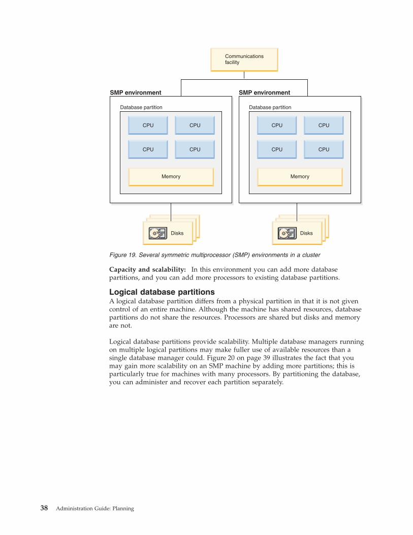
Capacity
and
scalability:
In
this
environment
you
can
add
more
database
partitions,
and
you
can
add
more
processors
to
existing
database
partitions.
Logical
database
partitions
A
logical
database
partition
differs
from
a
physical
partition
in
that
it
is
not
given
control
of
an
entire
machine.
Although
the
machine
has
shared
resources,
database
partitions
do
not
share
the
resources.
Processors
are
shared
but
disks
and
memory
are
not.
Logical
database
partitions
provide
scalability.
Multiple
database
managers
running
on
multiple
logical
partitions
may
make
fuller
use
of
available
resources
than
a
single
database
manager
could.
Figure
20
on
page
39
illustrates
the
fact
that
you
may
gain
more
scalability
on
an
SMP
machine
by
adding
more
partitions;
this
is
particularly
true
for
machines
with
many
processors.
By
partitioning
the
database,
you
can
administer
and
recover
each
partition
separately.
CPU
CPU
CPU
CPU
Memory
CPU
CPU
CPU
CPU
Memory
Communicationsfacility
SMP environment SMP environment
Disks Disks
Database partition Database partition
Figure
19.
Several
symmetric
multiprocessor
(SMP)
environments
in
a
cluster
38
Administration
Guide:
Planning

Figure
21
on
page
40
illustrates
the
fact
that
you
can
multiply
the
configuration
shown
in
Figure
20
to
increase
processing
power.
Disks Disks
Big SMP environment
Databasepartition 1
Databasepartition 2
Memory Memory
CPU CPU
CPU CPU
Communicationsfacility
Figure
20.
Partitioned
database
with
symmetric
multiprocessor
environment
Chapter
2.
Parallel
database
systems
39

Note:
The
ability
to
have
two
or
more
partitions
coexist
on
the
same
machine
(regardless
of
the
number
of
processors)
allows
greater
flexibility
in
designing
high
availability
configurations
and
failover
strategies.
Upon
machine
failure,
a
database
partition
can
be
automatically
moved
and
restarted
on
a
second
machine
that
already
contains
another
partition
of
the
same
database.
Summary
of
parallelism
best
suited
to
each
hardware
environment
The
following
table
summarizes
the
types
of
parallelism
best
suited
to
take
advantage
of
the
various
hardware
environments.
Table
3.
Types
of
Parallelism
Possible
in
Each
Hardware
Environment
Hardware
Environment
I/O
Parallelism
Intra-Query
Parallelism
Intra-
Partition
Parallelism
Inter-
Partition
Parallelism
Single
Partition,
Single
Processor
Yes
No(1)
No
Single
Partition,
Multiple
Processors
(SMP)
Yes
Yes
No
Multiple
Partitions,
One
Processor
(MPP)
Yes
No(1)
Yes
Communicationsfacility
Disks DisksDisks Disks
Big SMPenvironment
Big SMPenvironment
Databasepartition 1
Databasepartition 1
Databasepartition 2
Databasepartition 2
Memory MemoryMemory Memory
CPU CPUCPU CPU
CPU CPUCPU CPU
Communicationsfacility
Communicationsfacility
Figure
21.
Partitioned
database
with
symmetric
multiprocessor
environments
clustered
together
40
Administration
Guide:
Planning

Table
3.
Types
of
Parallelism
Possible
in
Each
Hardware
Environment
(continued)
Hardware
Environment
I/O
Parallelism
Intra-Query
Parallelism
Intra-
Partition
Parallelism
Inter-
Partition
Parallelism
Multiple
Partitions,
Multiple
Processors
(cluster
of
SMPs)
Yes
Yes
Yes
Logical
Database
Partitions
Yes
Yes
Yes
Note:
(1)
There
may
be
an
advantage
to
setting
the
degree
of
parallelism
(using
one
of
the
configuration
parameters)
to
some
value
greater
than
one,
even
on
a
single
processor
system,
especially
if
the
queries
you
execute
are
not
fully
utilizing
the
CPU
(for
example,
if
they
are
I/O
bound).
Related
concepts:
v
“Parallelism”
on
page
30
Chapter
2.
Parallel
database
systems
41

42
Administration
Guide:
Planning

Chapter
3.
About
data
warehousing
What
solutions
does
data
warehousing
provide?
The
systems
that
contain
operational
data
(the
data
that
runs
the
daily
transactions
of
your
business)
contain
information
that
is
useful
to
business
analysts.
For
example,
analysts
can
use
information
about
which
products
were
sold
in
which
regions
at
which
time
of
year
to
look
for
anomalies
or
to
project
future
sales.
However,
several
problems
can
arise
when
analysts
access
the
operational
data
directly:
v
Analysts
might
not
have
the
expertise
to
query
the
operational
database.
For
example,
querying
IMS™
databases
requires
an
application
program
that
uses
a
specialized
type
of
data
manipulation
language.
In
general,
the
programmers
who
have
the
expertise
to
query
the
operational
database
have
a
full-time
job
in
maintaining
the
database
and
its
applications.
v
Performance
is
critical
for
many
operational
databases,
such
as
databases
for
a
bank.
The
system
cannot
handle
users
making
ad
hoc
queries.
v
The
operational
data
generally
is
not
in
the
best
format
for
use
by
business
analysts.
For
example,
sales
data
that
is
summarized
by
product,
region,
and
season
is
much
more
useful
to
analysts
than
the
raw
data.
Data
warehousing
solves
these
problems.
In
data
warehousing,
you
create
stores
of
informational
data.
Informational
data
is
data
that
is
extracted
from
the
operational
data
and
then
transformed
for
decision
making.
For
example,
a
data
warehousing
tool
might
copy
all
the
sales
data
from
the
operational
database,
clean
the
data,
perform
calculations
to
summarize
the
data,
and
write
the
summarized
data
to
a
target
in
a
separate
database
from
the
operational
data.
Users
can
query
the
separate
database
(the
warehouse)
without
impacting
the
operational
databases.
Related
concepts:
v
“Data
warehouse
objects”
on
page
43
Data
warehouse
objects
The
following
sections
describe
the
objects
that
you
will
use
to
create
and
maintain
your
data
warehouse.
Operationaldata
ExtractCleanseTransform
Informationaldata
Dataanalysis
Figure
22.
The
path
from
operational
data
to
data
analysis
©
Copyright
IBM
Corp.
1993
-
2004
43

Subject
areas
A
subject
area
identifies
and
groups
the
processes
that
relate
to
a
logical
area
of
the
business.
For
example,
if
you
are
building
a
warehouse
of
marketing
and
sales
data,
you
define
a
Sales
subject
area
and
a
Marketing
subject
area.
You
then
add
the
processes
that
relate
to
sales
under
the
Sales
subject
area.
Similarly,
you
add
the
definitions
that
relate
to
the
marketing
data
under
the
Marketing
subject
area.
Warehouse
sources
Warehouse
sources
identify
the
tables
and
files
that
will
provide
data
to
your
warehouse.
The
Data
Warehouse
Center
uses
the
specifications
in
the
warehouse
sources
to
access
the
data.
The
sources
can
be
almost
any
relational
or
nonrelational
source
(table,
view,
or
file),
or
WebSphere®
Site
Analyzer
source
that
has
connectivity
to
your
network.
Warehouse
targets
Warehouse
targets
are
database
tables
or
files
that
contain
data
that
has
been
transformed.
You
can
use
warehouse
targets
to
provide
data
to
other
warehouse
targets.
For
example,
a
central
warehouse
can
provide
data
to
departmental
servers,
or
a
main
fact
table
in
the
warehouse
can
provide
data
to
summary
tables.
Warehouse
control
databases
The
warehouse
control
database
contains
the
control
tables
that
are
required
to
store
the
Data
Warehouse
Center
metadata.
Starting
in
the
Data
Warehouse
Center
Version
8.2,
the
warehouse
control
database
must
be
a
UTF-8
(Unicode
Transformation
Format,
or
Unicode)
database.
This
requirement
provides
expanded
language
support
for
the
Data
Warehouse
Center.
If
you
try
to
log
on
to
the
Data
Warehouse
Center
using
a
database
that
is
not
in
Unicode
format,
you
will
receive
an
error
message
that
you
cannot
log
on.
You
can
use
the
Warehouse
Control
Database
Management
tool
to
migrate
the
metadata
from
a
specified
database
into
a
new
Unicode
database.
Warehouse
agents
and
agent
sites
Warehouse
agents
manage
the
flow
of
data
between
the
data
sources
and
the
target
warehouses.
Warehouse
agents
are
available
on
the
AIX®,
Linux,
iSeries™,
z/OS™,
Windows®
NT,
Windows
2000,
and
Windows
XP
operating
systems,
and
for
the
Solaris™
Operating
Environment.
The
agents
use
Open
Database
Connectivity
(ODBC)
drivers
or
DB2®
CLI
to
communicate
with
different
databases.
Informationaldata
Warehousetarget
Warehousesource
Steps
Process
Subject area
Operationaldata
Figure
23.
The
hierarchy
of
subject
areas
44
Administration
Guide:
Planning
|
|||
|||||
|
|||||||||

Several
agents
can
handle
the
transfer
of
data
between
sources
and
target
warehouses.
The
number
of
agents
that
you
use
depends
on
your
existing
connectivity
configuration
and
the
volume
of
data
that
you
plan
to
move
to
your
warehouse.
Additional
instances
of
an
agent
can
be
generated
if
multiple
processes
that
require
the
same
agent
are
running
simultaneously.
Agents
can
be
local
or
remote.
A
local
warehouse
agent
is
an
agent
that
is
installed
on
the
same
workstation
as
the
warehouse
server.
A
remote
warehouse
agent
is
an
agent
that
is
installed
on
another
workstation
that
has
connectivity
to
the
warehouse
server.
An
agent
site
is
a
logical
name
for
a
workstation
where
agent
software
is
installed.
The
agent
site
name
is
not
the
same
as
the
TCP/IP
host
name.
A
single
workstation
can
have
only
one
TCP/IP
host
name.
However,
you
can
define
multiple
agent
sites
on
a
single
workstation.
A
logical
name
identifies
each
agent
site.
The
default
agent
site,
named
the
Default
DWC
Agent
Site,
is
a
local
agent
that
the
Data
Warehouse
Center
defines
during
initialization
of
the
warehouse
control
database.
Processes
and
steps
A
process
contains
a
series
of
steps
that
performs
a
transformation
and
movement
of
data
for
a
specific
warehouse
use.
In
general,
a
process
moves
source
data
into
the
warehouse.
Then,
the
data
is
aggregated
and
summarized
for
warehouse
use.
A
process
can
produce
a
single
flat
table
or
a
set
of
summary
tables.
A
process
might
also
perform
some
specific
type
of
data
transformation.
A
step
is
the
definition
of
a
single
operation
within
the
warehouse.
By
using
SQL
statements
or
calling
programs,
steps
define
how
you
move
data
and
transform
data.
When
you
run
a
step,
a
transfer
of
data
between
the
warehouse
source
and
the
warehouse
target,
or
any
transformation
of
that
data,
can
take
place.
A
step
is
a
logical
entity
in
the
Data
Warehouse
Center
that
defines:
v
A
link
to
its
source
data.
v
The
definition
of
and
a
link
to
the
output
table
or
file.
v
The
mechanism
(either
an
SQL
statement
or
a
program)
and
definition
for
populating
the
output
table
or
file.
Data WarehouseCenter GUI
Datasources
Agentslocal or remote
Targetwarehouse
Warehouseserver
Figure
24.
The
relationship
between
agents,
data
sources,
target
warehouses,
and
the
warehouse
server
Chapter
3.
About
data
warehousing
45
|||||
||||

v
The
processing
options
and
schedule
by
which
the
output
table
or
file
is
populated.
Suppose
that
you
want
Data
Warehouse
Center
to
perform
the
following
tasks:
1.
Extract
data
from
different
databases.
2.
Convert
the
data
to
a
single
format.
3.
Write
the
data
to
a
table
in
a
data
warehouse.
You
would
create
a
process
that
contains
several
steps.
Each
step
performs
a
separate
task,
such
as
extracting
the
data
from
a
database
or
converting
it
to
the
correct
format.
You
might
need
to
create
several
steps
to
completely
transform
and
format
the
data
and
put
it
into
its
final
table.
When
a
step
or
a
process
runs,
it
can
affect
the
target
in
the
following
ways:
v
Replace
all
the
data
in
the
warehouse
target
with
new
data
v
Append
the
new
data
to
the
existing
data
v
Append
a
separate
edition
of
data
v
Update
existing
data
You
can
run
a
step
on
demand,
or
you
can
schedule
a
step
to
run:
v
At
a
set
time
v
Only
one
time
v
Repeatedly,
such
as
every
Friday
v
In
Sequence,
so
that
when
one
step
finishes
running,
the
next
step
begins
running
v
Upon
completion,
either
successful
or
not
successful,
of
another
step
If
you
schedule
a
process,
the
first
step
in
the
process
runs
at
the
scheduled
time.
The
following
sections
describe
the
various
types
of
steps
that
you
will
find
in
the
Data
Warehouse
Center.
SQL
steps
The
Data
Warehouse
Center
provides
two
types
of
SQL
steps.
The
SQL
Select
and
Insert
step
uses
an
SQL
SELECT
statement
to
extract
data
from
a
warehouse
source
and
generates
an
INSERT
statement
to
insert
the
data
into
the
warehouse
target
table.
The
SQL
Select
and
Update
step
uses
an
SQL
SELECT
statement
to
extract
data
from
a
warehouse
source
and
update
existing
data
in
the
warehouse
target
table.
Program
steps
The
Data
Warehouse
Center
provides
several
types
of
program
steps:
DB2
for
iSeries
programs,
DB2
for
z/OS
programs,
DB2
Universal
Database™
programs,
Visual
Warehouse™
5.2
DB2
programs,
OLAP
Server
programs,
File
programs,
and
Replication
programs.
These
steps
run
predefined
programs
and
utilities.
The
warehouse
programs
for
a
particular
operating
system
are
packaged
with
the
agent
for
that
operating
system.
You
install
the
warehouse
programs
when
you
install
the
agent
code.
46
Administration
Guide:
Planning
|
|
|
||
|
||||||
|||||||

Transformer
steps
Transformer
steps
are
stored
procedures
and
user-defined
functions
that
specify
statistical
or
warehouse
transformers
that
you
can
use
to
transform
data.
You
can
use
transformers
to
clean,
invert,
and
pivot
data;
generate
primary
keys
and
period
tables;
and
calculate
various
statistics.
In
a
transformer
step,
you
specify
one
of
the
statistical
or
warehouse
transformers.
When
you
run
the
process,
the
transformer
step
writes
data
to
one
or
more
warehouse
targets.
User-defined
program
steps
A
user-defined
program
step
is
a
logical
entity
within
the
Data
Warehouse
Center
that
represents
a
business-specific
transformation
that
you
want
the
Data
Warehouse
Center
to
start.
Because
every
business
has
unique
data
transformation
requirements,
businesses
can
choose
to
write
their
own
program
steps
or
to
use
tools
such
as
those
provided
by
other
companies,
such
as
ETI
or
Vality.
For
example,
you
can
write
a
user-defined
program
that
will
perform
the
following
functions:
1.
Export
data
from
a
table.
2.
Manipulate
that
data.
3.
Write
the
data
to
a
temporary
output
resource
or
a
warehouse
target.
Related
concepts:
v
“What
solutions
does
data
warehousing
provide?”
on
page
43
v
“Warehouse
tasks”
on
page
47
v
“What
is
a
user-defined
program?”
in
the
Data
Warehouse
Center
Administration
Guide
v
“What
is
a
program
group?”
in
the
Data
Warehouse
Center
Administration
Guide
Warehouse
tasks
Creating
a
data
warehouse
involves
the
following
tasks:
v
Identifying
the
source
data
(or
operational
data)
and
defining
it
for
use
as
warehouse
sources.
v
Creating
a
database
to
use
as
the
warehouse
and
defining
warehouse
targets.
v
Defining
a
subject
area
for
groups
of
processes
that
you
will
define
in
your
warehouse.
v
Specifying
how
to
move
and
transform
the
source
data
into
its
format
for
the
warehouse
database
by
defining
steps
in
the
processes.
v
Testing
the
steps
that
you
define
and
scheduling
them
to
run
automatically.
v
Administering
the
warehouse
by
defining
security
and
monitoring
database
usage
using
the
Work
in
Progress
notebook.
If
you
have
DB2®
Warehouse
Manager,
you
can
create
an
information
catalog
of
the
data
in
the
warehouse.
An
information
catalog
is
a
database
that
contains
business
metadata.
Business
metadata
helps
users
identify
and
locate
data
and
information
available
to
them
in
the
organization.
Data
Warehouse
Metadata
can
be
published
to
the
information
catalog.
The
information
catalog
can
be
searched
to
determine
what
data
is
available
in
the
warehouse.
Chapter
3.
About
data
warehousing
47
||||||

You
can
also
define
a
star
schema
model
for
the
data
in
the
warehouse.
A
star
schema
is
a
specialized
design
that
consists
of
multiple
dimension
tables,
which
describe
aspects
of
a
business,
and
one
fact
table,
which
contains
the
facts
or
measurements
about
the
business.
For
example,
for
a
manufacturing
company,
some
dimension
tables
are
products,
markets,
and
time.
The
fact
table
contains
transaction
information
about
the
products
that
are
ordered
in
each
region
by
season.
Related
concepts:
v
“Warehouse
steps”
in
the
Data
Warehouse
Center
Administration
Guide
Related
tasks:
v
“Steps
and
tasks:
Data
Warehouse
Center
help”
48
Administration
Guide:
Planning
|||||||

Part
2.
Database
design
©
Copyright
IBM
Corp.
1993
-
2004
49

50
Administration
Guide:
Planning

Chapter
4.
Logical
database
design
Your
goal
in
designing
a
database
is
to
produce
a
representation
of
your
environment
that
is
easy
to
understand
and
that
will
serve
as
a
basis
for
expansion.
In
addition,
you
want
a
database
design
that
will
help
you
maintain
consistency
and
integrity
of
your
data.
You
can
do
this
by
producing
a
design
that
will
reduce
redundancy
and
eliminate
anomalies
that
can
occur
during
the
updating
of
your
database.
Database
design
is
not
a
linear
process;
you
will
probably
have
to
redo
steps
as
you
work
out
the
design.
What
to
record
in
a
database
The
first
step
in
developing
a
database
design
is
to
identify
the
types
of
data
to
be
stored
in
database
tables.
A
database
includes
information
about
the
entities
in
an
organization
or
business,
and
their
relationships
to
each
other.
In
a
relational
database,
entities
are
represented
as
tables.
An
entity
is
a
person,
object,
or
concept
about
which
you
want
to
store
information.
Some
of
the
entities
described
in
the
sample
tables
are
employees,
departments,
and
projects.
In
the
sample
employee
table,
the
entity
″employee″
has
attributes,
or
properties,
such
as
employee
number,
name,
work
department,
and
salary
amount.
Those
properties
appear
as
the
columns
EMPNO,
FIRSTNME,
LASTNAME,
WORKDEPT,
and
SALARY.
An
occurrence
of
the
entity
″employee″
consists
of
the
values
in
all
of
the
columns
for
one
employee.
Each
employee
has
a
unique
employee
number
(EMPNO)
that
can
be
used
to
identify
an
occurrence
of
the
entity
″employee″.
Each
row
in
a
table
represents
an
occurrence
of
an
entity
or
relationship.
For
example,
in
the
following
table
the
values
in
the
first
row
describe
an
employee
named
Haas.
Table
4.
Occurrences
of
Employee
Entities
and
their
Attributes
EMPNO
FIRSTNME
LASTNAME
WORKDEPT
JOB
000010
Christine
Haas
A00
President
000020
Michael
Thompson
B01
Manager
000120
Sean
O’Connell
A00
Clerk
000130
Dolores
Quintana
C01
Analyst
000030
Sally
Kwan
C01
Manager
000140
Heather
Nicholls
C01
Analyst
000170
Masatoshi
Yoshimura
D11
Designer
There
is
a
growing
need
to
support
non-traditional
database
applications
such
as
multimedia.
You
may
want
to
consider
attributes
to
support
multimedia
objects
such
as
documents,
video
or
mixed
media,
image,
and
voice.
©
Copyright
IBM
Corp.
1993
-
2004
51

Within
a
table,
each
column
of
a
row
is
related
in
some
way
to
all
the
other
columns
of
that
row.
Some
of
the
relationships
expressed
in
the
sample
tables
are:
v
Employees
are
assigned
to
departments
–
Dolores
Quintana
is
assigned
to
Department
C01v
Employees
perform
a
job
–
Dolores
works
as
an
Analystv
Employees
manage
departments
–
Sally
manages
department
C01.
″Employee″
and
″department″
are
entities;
Sally
Kwan
is
part
of
an
occurrence
of
″employee,″
and
C01
is
part
of
an
occurrence
of
″department″.
The
same
relationship
applies
to
the
same
columns
in
every
row
of
a
table.
For
example,
one
row
of
a
table
expresses
the
relationship
that
Sally
Kwan
manages
Department
C01;
another,
the
relationship
that
Sean
O’Connell
is
a
clerk
in
Department
A00.
The
information
contained
within
a
table
depends
on
the
relationships
to
be
expressed,
the
amount
of
flexibility
needed,
and
the
data
retrieval
speed
desired.
In
addition
to
identifying
the
entity
relationships
within
your
enterprise,
you
also
need
to
identify
other
types
of
information,
such
as
the
business
rules
that
apply
to
that
data.
Related
concepts:
v
“Database
relationships”
on
page
52
v
“Column
definitions”
on
page
55
Database
relationships
Several
types
of
relationships
can
be
defined
in
a
database.
Consider
the
possible
relationships
between
employees
and
departments.
One-to-many
and
many-to-one
relationships
An
employee
can
work
in
only
one
department;
this
relationship
is
single-valued
for
employees.
On
the
other
hand,
one
department
can
have
many
employees;
this
relationship
is
multi-valued
for
departments.
The
relationship
between
employees
(single-valued)
and
departments
(multi-valued)
is
a
one-to-many
relationship.
To
define
tables
for
each
one-to-many
and
each
many-to-one
relationship:
1.
Group
all
the
relationships
for
which
the
″many″
side
of
the
relationship
is
the
same
entity.
2.
Define
a
single
table
for
all
the
relationships
in
the
group.
In
the
following
example,
the
″many″
side
of
the
first
and
second
relationships
is
″employees″
so
an
employee
table,
EMPLOYEE,
is
defined.
Table
5.
Many-to-One
Relationships
Entity
Relationship
Entity
Employees
are
assigned
to
departments
Employees
work
at
jobs
Departments
report
to
(administrative)
departments
52
Administration
Guide:
Planning
||

In
the
third
relationship,
″departments″
is
on
the
″many″
side,
so
a
department
table,
DEPARTMENT,
is
defined.
The
following
tables
show
these
different
relationships.
The
EMPLOYEE
table:
EMPNO
WORKDEPT
JOB
000010
A00
President
000020
B01
Manager
000120
A00
Clerk
000130
C01
Analyst
000030
C01
Manager
000140
C01
Analyst
000170
D11
Designer
The
DEPARTMENT
table:
DEPTNO
ADMRDEPT
C01
A00
D01
A00
D11
D01
Many-to-many
relationships
A
relationship
that
is
multi-valued
in
both
directions
is
a
many-to-many
relationship.
An
employee
can
work
on
more
than
one
project,
and
a
project
can
have
more
than
one
employee.
The
questions
″What
does
Dolores
Quintana
work
on?″,
and
″Who
works
on
project
IF1000?″
both
yield
multiple
answers.
A
many-to-many
relationship
can
be
expressed
in
a
table
with
a
column
for
each
entity
(″employees″
and
″projects″),
as
shown
in
the
following
example.
The
following
table
shows
how
a
many-to-many
relationship
(an
employee
can
work
on
many
projects,
and
a
project
can
have
many
employees
working
on
it)
is
represented.
The
employee
activity
(EMP_ACT)
table:
EMPNO
PROJNO
000030
IF1000
000030
IF2000
000130
IF1000
000140
IF2000
000250
AD3112
One-to-one
relationships
One-to-one
relationships
are
single-valued
in
both
directions.
A
manager
manages
one
department;
a
department
has
only
one
manager.
The
questions,
″Who
is
the
manager
of
Department
C01?″,
and
″What
department
does
Sally
Kwan
manage?″
Chapter
4.
Logical
database
design
53
||
|
|||

both
have
single
answers.
The
relationship
can
be
assigned
to
either
the
DEPARTMENT
table
or
the
EMPLOYEE
table.
Because
all
departments
have
managers,
but
not
all
employees
are
managers,
it
is
most
logical
to
add
the
manager
to
the
DEPARTMENT
table,
as
shown
in
the
following
example.
The
following
table
shows
the
representation
of
a
one-to-one
relationship.
The
DEPARTMENT
table:
DEPTNO
MGRNO
A00
000010
B01
000020
D11
000060
Ensure
that
equal
values
represent
the
same
entity
You
can
have
more
than
one
table
describing
the
attributes
of
the
same
set
of
entities.
For
example,
the
EMPLOYEE
table
shows
the
number
of
the
department
to
which
an
employee
is
assigned,
and
the
DEPARTMENT
table
shows
which
manager
is
assigned
to
each
department
number.
To
retrieve
both
sets
of
attributes
simultaneously,
you
can
join
the
two
tables
on
the
matching
columns,
as
shown
in
the
following
example.
The
values
in
WORKDEPT
and
DEPTNO
represent
the
same
entity,
and
represent
a
join
path
between
the
DEPARTMENT
and
EMPLOYEE
tables.
The
DEPARTMENT
table:
DEPTNO
DEPTNAME
MGRNO
ADMRDEPT
D21
Administration
Support
000070
D01
The
EMPLOYEE
table:
EMPNO
FIRSTNAME
LASTNAME
WORKDEPT
JOB
000250
Daniel
Smith
D21
Clerk
When
you
retrieve
information
about
an
entity
from
more
than
one
table,
ensure
that
equal
values
represent
the
same
entity.
The
connecting
columns
can
have
different
names
(like
WORKDEPT
and
DEPTNO
in
the
previous
example),
or
they
can
have
the
same
name
(like
the
columns
called
DEPTNO
in
the
department
and
project
tables).
Related
concepts:
v
“What
to
record
in
a
database”
on
page
51
v
“Column
definitions”
on
page
55
54
Administration
Guide:
Planning
|

Column
definitions
To
define
a
column
in
a
relational
table:
1.
Choose
a
name
for
the
column.
Each
column
in
a
table
must
have
a
name
that
is
unique
for
that
table.
2.
State
what
kind
of
data
is
valid
for
the
column.
The
data
type
and
length
specify
the
type
of
data
and
the
maximum
length
that
are
valid
for
the
column.
Data
types
may
be
chosen
from
those
provided
by
the
database
manager
or
you
may
choose
to
create
your
own
user-defined
types.
Examples
of
data
type
categories
are:
numeric,
character
string,
double-byte
(or
graphic)
character
string,
date-time,
and
binary
string.
Large
object
(LOB)
data
types
support
multi-media
objects
such
as
documents,
video,
image
and
voice.
These
objects
are
implemented
using
the
following
data
types:
v
A
binary
large
object
(BLOB)
string.
Examples
of
BLOBs
are
photographs
of
employees,
voice,
and
video.
v
A
character
large
object
(CLOB)
string,
where
the
sequence
of
characters
can
be
either
single-
or
multi-byte
characters,
or
a
combination
of
both.
An
example
of
a
CLOB
is
an
employee’s
resume.
v
A
double-byte
character
large
object
(DBCLOB)
string,
where
the
sequence
of
characters
is
double-byte
characters.
An
example
of
a
DBCLOB
is
a
Japanese
resume.
A
user-defined
type
(UDT),
is
a
type
that
is
derived
from
an
existing
type.
You
may
need
to
define
types
that
are
derived
from
and
share
characteristics
with
existing
types,
but
that
are
nevertheless
considered
to
be
separate
and
incompatible.
A
structured
type
is
a
user-defined
type
whose
structure
is
defined
in
the
database.
It
contains
a
sequence
of
named
attributes,
each
of
which
has
a
data
type.
A
structured
type
may
be
defined
as
a
subtype
of
another
structured
type,
called
its
supertype.
A
subtype
inherits
all
the
attributes
of
its
supertype
and
may
have
additional
attributes
defined.
The
set
of
structured
types
that
are
related
to
a
common
supertype
is
called
a
type
hierarchy,
and
the
supertype
that
does
not
have
any
supertype
is
called
the
root
type
of
the
type
hierarchy.
A
structured
type
may
be
used
as
the
type
of
a
table
or
a
view.
The
names
and
data
types
of
the
attributes
of
the
structured
types,
together
with
the
object
identifier,
become
the
names
and
data
types
of
the
columns
of
this
typed
table
or
typed
view.
Rows
of
the
typed
table
or
typed
view
can
be
thought
of
as
a
representation
of
instances
of
the
structured
type.
A
structured
type
cannot
be
used
as
the
data
type
of
a
column
of
a
table
or
a
view.
There
is
also
no
support
for
retrieving
a
whole
structured
type
instance
into
a
host
variable
in
an
application
program.
A
reference
type
is
a
companion
type
to
the
structured
type.
Similar
to
a
distinct
type,
a
reference
type
is
a
scalar
type
that
shares
a
common
representation
with
one
of
the
built-in
data
types.
This
same
representation
is
shared
for
all
types
in
the
type
hierarchy.
The
reference
type
representation
is
defined
when
the
root
type
of
a
type
hierarchy
is
created.
When
using
a
reference
type,
a
structured
type
is
specified
as
a
parameter
of
the
type.
This
parameter
is
called
the
target
type
of
the
reference.
The
target
of
a
reference
is
always
a
row
in
a
typed
table
or
view.
When
a
reference
type
is
used,
it
may
have
a
scope
defined.
The
scope
identifies
a
table
(called
the
target
table)
or
view
(called
the
target
view)
that
contains
the
target
row
of
a
reference
value.
The
target
table
or
view
must
have
the
same
type
as
Chapter
4.
Logical
database
design
55

the
target
type
of
the
reference
type.
An
instance
of
a
scoped
reference
type
uniquely
identifies
a
row
in
a
typed
table
or
typed
view,
called
its
target
row.
A
user-defined
function
(UDF)
can
be
used
for
a
number
of
reasons,
including
invoking
routines
that
allow
comparison
or
conversion
between
user-defined
types.
UDFs
extend
and
add
to
the
support
provided
by
built-in
SQL
functions,
and
can
be
used
wherever
a
built-in
function
can
be
used.
There
are
two
types
of
UDFs:
v
An
external
function,
which
is
written
in
a
programming
language
v
A
sourced
function,
which
will
be
used
to
invoke
other
UDFs
For
example,
two
numeric
data
types
are
European
Shoe
Size
and
American
Shoe
Size.
Both
types
represent
shoe
size,
but
they
are
incompatible,
because
the
measurement
base
is
different
and
cannot
be
compared.
A
user-defined
function
can
be
invoked
to
convert
one
shoe
size
to
another.
3.
State
which
columns
might
need
default
values.
Some
columns
cannot
have
meaningful
values
in
all
rows
because:
v
A
column
value
is
not
applicable
to
the
row.
For
example,
a
column
containing
an
employee’s
middle
initial
is
not
applicable
to
an
employee
who
has
no
middle
initial.
v
A
value
is
applicable,
but
is
not
yet
known.
For
example,
the
MGRNO
column
might
not
contain
a
valid
manager
number
because
the
previous
manager
of
the
department
has
been
transferred,
and
a
new
manager
has
not
been
appointed
yet.
In
both
situations,
you
can
choose
between
allowing
a
NULL
value
(a
special
value
indicating
that
the
column
value
is
unknown
or
not
applicable),
or
allowing
a
non-NULL
default
value
to
be
assigned
by
the
database
manager
or
by
the
application.
Primary
keys
A
key
is
a
set
of
columns
that
can
be
used
to
identify
or
access
a
particular
row
or
rows.
The
key
is
identified
in
the
description
of
a
table,
index,
or
referential
constraint.
The
same
column
can
be
part
of
more
than
one
key.
A
unique
key
is
a
key
that
is
constrained
so
that
no
two
of
its
values
are
equal.
The
columns
of
a
unique
key
cannot
contain
NULL
values.
For
example,
an
employee
number
column
can
be
defined
as
a
unique
key,
because
each
value
in
the
column
identifies
only
one
employee.
No
two
employees
can
have
the
same
employee
number.
The
mechanism
used
to
enforce
the
uniqueness
of
the
key
is
called
a
unique
index.
The
unique
index
of
a
table
is
a
column,
or
an
ordered
collection
of
columns,
for
which
each
value
identifies
(functionally
determines)
a
unique
row.
A
unique
index
can
contain
NULL
values.
The
primary
key
is
one
of
the
unique
keys
defined
on
a
table,
but
is
selected
to
be
the
key
of
first
importance.
There
can
be
only
one
primary
key
on
a
table.
A
primary
index
is
automatically
created
for
the
primary
key.
The
primary
index
is
used
by
the
database
manager
for
efficient
access
to
table
rows,
and
allows
the
database
manager
to
enforce
the
uniqueness
of
the
primary
key.
(You
can
also
define
indexes
on
non-primary
key
columns
to
efficiently
access
data
when
processing
queries.)
56
Administration
Guide:
Planning

If
a
table
does
not
have
a
″natural″
unique
key,
or
if
arrival
sequence
is
the
method
used
to
distinguish
unique
rows,
using
a
time
stamp
as
part
of
the
key
can
be
helpful.
Primary
keys
for
some
of
the
sample
tables
are:
Table
Key
Column
Employee
table
EMPNO
Department
table
DEPTNO
Project
table
PROJNO
The
following
example
shows
part
of
the
PROJECT
table,
including
its
primary
key
column.
Table
6.
A
Primary
Key
on
the
PROJECT
Table
PROJNO
(Primary
Key)
PROJNAME
DEPTNO
MA2100
Weld
Line
Automation
D01
MA2110
Weld
Line
Programming
D11
If
every
column
in
a
table
contains
duplicate
values,
you
cannot
define
a
primary
key
with
only
one
column.
A
key
with
more
than
one
column
is
a
composite
key.
The
combination
of
column
values
should
define
a
unique
entity.
If
a
composite
key
cannot
be
easily
defined,
you
may
consider
creating
a
new
column
that
has
unique
values.
The
following
example
shows
a
primary
key
containing
more
than
one
column
(a
composite
key):
Table
7.
A
Composite
Primary
Key
on
the
EMP_ACT
Table
EMPNO
(Primary
Key)
PROJNO
(Primary
Key)
ACTNO
(Primary
Key)
EMPTIME
EMSTDATE
(Primary
Key)
000250
AD3112
60
1.0
1982-01-01
000250
AD3112
60
.5
1982-02-01
000250
AD3112
70
.5
1982-02-01
Identifying
candidate
key
columns
To
identify
candidate
keys,
select
the
smallest
number
of
columns
that
define
a
unique
entity.
There
may
be
more
than
one
candidate
key.
In
Table
8,
there
appear
to
be
many
candidate
keys.
The
EMPNO,
the
PHONENO,
and
the
LASTNAME
columns
each
uniquely
identify
the
employee.
Table
8.
EMPLOYEE
Table
EMPNO
(Primary
Key)
FIRSTNAME
LASTNAME
WORKDEPT
(Foreign
Key)
PHONENO
000010
Christine
Haas
A00
3978
000030
Sally
Kwan
C01
4738
000060
Irving
Stern
D11
6423
000120
Sean
O’Connell
A00
2167
000140
Heather
Nicholls
C01
1793
Chapter
4.
Logical
database
design
57

Table
8.
EMPLOYEE
Table
(continued)
EMPNO
(Primary
Key)
FIRSTNAME
LASTNAME
WORKDEPT
(Foreign
Key)
PHONENO
000170
Masatoshi
Yoshimura
D11
2890
The
criteria
for
selecting
a
primary
key
from
a
pool
of
candidate
keys
should
be
persistence,
uniqueness,
and
stability:
v
Persistence
means
that
a
primary
key
value
for
each
row
always
exists.
v
Uniqueness
means
that
the
key
value
for
each
row
is
different
from
all
the
others.
v
Stability
means
that
primary
key
values
never
change.
Of
the
three
candidate
keys
in
the
example,
only
EMPNO
satisfies
all
of
these
criteria.
An
employee
may
not
have
a
phone
number
when
joining
a
company.
Last
names
can
change,
and,
although
they
may
be
unique
at
one
point,
are
not
guaranteed
to
be
so.
The
employee
number
column
is
the
best
choice
for
the
primary
key.
An
employee
is
assigned
a
unique
number
only
once,
and
that
number
is
generally
not
updated
as
long
as
the
employee
remains
with
the
company.
Since
each
employee
must
have
a
number,
values
in
the
employee
number
column
are
persistent.
Related
concepts:
v
“Identity
columns”
on
page
58
Identity
columns
An
identity
column
provides
a
way
for
DB2®
Universal
Database
(DB2
UDB)
to
automatically
generate
a
unique
numeric
value
for
each
row
in
a
table.
A
table
can
have
a
single
column
that
is
defined
with
the
identity
attribute.
Examples
of
an
identity
column
include
order
number,
employee
number,
stock
number,
and
incident
number.
Values
for
an
identity
column
can
be
generated
always
or
by
default.
v
An
identity
column
that
is
defined
as
generated
always
is
guaranteed
to
be
unique
by
DB2
UDB.
Its
values
are
always
generated
by
DB2
UDB;
applications
are
not
allowed
to
provide
an
explicit
value.
v
An
identity
column
that
is
defined
as
generated
by
default
gives
applications
a
way
to
explicitly
provide
a
value
for
the
identity
column.
If
a
value
is
not
given,
DB2
UDB
generates
one,
but
cannot
guarantee
the
uniqueness
of
the
value
in
this
case.
DB2
UDB
guarantees
uniqueness
only
for
the
set
of
values
that
it
generates.
Generated
by
default
is
meant
to
be
used
for
data
propagation,
in
which
the
contents
of
an
existing
table
are
copied,
or
for
the
unloading
and
reloading
of
a
table.
Identity
columns
are
ideally
suited
to
the
task
of
generating
unique
primary
key
values.
Applications
can
use
identity
columns
to
avoid
the
concurrency
and
performance
problems
that
can
result
when
an
application
generates
its
own
unique
counter
outside
of
the
database.
For
example,
one
common
application-level
implementation
is
to
maintain
a
1-row
table
containing
a
counter.
Each
transaction
locks
this
table,
increments
the
number,
and
then
commits;
that
is,
only
one
transaction
at
a
time
can
increment
the
counter.
In
contrast,
if
the
counter
is
maintained
through
an
identity
column,
much
higher
levels
of
concurrency
can
58
Administration
Guide:
Planning
|||||
|||
|||||||

be
achieved
because
the
counter
is
not
locked
by
transactions.
One
uncommitted
transaction
that
has
incremented
the
counter
will
not
prevent
subsequent
transactions
from
also
incrementing
the
counter.
The
counter
for
the
identity
column
is
incremented
(or
decremented)
independently
of
the
transaction.
If
a
given
transaction
increments
an
identity
counter
two
times,
that
transaction
may
see
a
gap
in
the
two
numbers
that
are
generated
because
there
may
be
other
transactions
concurrently
incrementing
the
same
identity
counter
(that
is,
inserting
rows
into
the
same
table).
If
an
application
must
have
a
consecutive
range
of
numbers,
that
application
should
take
an
exclusive
lock
on
the
table
that
has
the
identity
column.
This
decision
must
be
weighed
against
the
resulting
loss
of
concurrency.
Furthermore,
it
is
possible
that
a
given
identity
column
can
appear
to
have
generated
gaps
in
the
number,
because
a
transaction
that
generated
a
value
for
the
identity
column
has
rolled
back,
or
the
database
that
has
cached
a
range
of
values
has
been
deactivated
before
all
of
the
cached
values
were
assigned.
The
sequential
numbers
that
are
generated
by
the
identity
column
have
the
following
additional
properties:
v
The
values
can
be
of
any
exact
numeric
data
type
with
a
scale
of
zero;
that
is,
SMALLINT,
INTEGER,
BIGINT,
or
DECIMAL
with
a
scale
of
zero.
(Single-
and
double-precision
floating-point
are
considered
to
be
approximate
numeric
data
types.)
v
Consecutive
values
can
differ
by
any
specified
integer
increment.
The
default
increment
is
1.
v
The
counter
value
for
the
identity
column
is
recoverable.
If
a
failure
occurs,
the
counter
value
is
reconstructed
from
the
logs,
thereby
guaranteeing
that
unique
values
continue
to
be
generated.
v
Identity
column
values
can
be
cached
to
give
better
performance.
Related
concepts:
v
“Primary
keys”
on
page
56
Normalization
Normalization
helps
eliminate
redundancies
and
inconsistencies
in
table
data.
It
is
the
process
of
reducing
tables
to
a
set
of
columns
where
all
the
non-key
columns
depend
on
the
primary
key
column.
If
this
is
not
the
case,
the
data
can
become
inconsistent
during
updates.
This
section
briefly
reviews
the
rules
for
first,
second,
third,
and
fourth
normal
form.
The
fifth
normal
form
of
a
table,
which
is
covered
in
many
books
on
database
design,
is
not
described
here.
Form
Description
First
At
each
row
and
column
position
in
the
table,
there
exists
one
value,
never
a
set
of
values.
Second
Each
column
that
is
not
part
of
the
key
is
dependent
upon
the
key.
Third
Each
non-key
column
is
independent
of
other
non-key
columns,
and
is
dependent
only
upon
the
key.
Fourth
No
row
contains
two
or
more
independent
multi-valued
facts
about
an
entity.
Chapter
4.
Logical
database
design
59

First
normal
form
A
table
is
in
first
normal
form
if
there
is
only
one
value,
never
a
set
of
values,
in
each
cell.
A
table
that
is
in
first
normal
form
does
not
necessarily
satisfy
the
criteria
for
higher
normal
forms.
For
example,
the
following
table
violates
first
normal
form
because
the
WAREHOUSE
column
contains
several
values
for
each
occurrence
of
PART.
Table
9.
Table
Violating
First
Normal
Form
PART
(Primary
Key)
WAREHOUSE
P0010
Warehouse
A,
Warehouse
B,
Warehouse
C
P0020
Warehouse
B,
Warehouse
D
The
following
example
shows
the
same
table
in
first
normal
form.
Table
10.
Table
Conforming
to
First
Normal
Form
PART
(Primary
Key)
WAREHOUSE
(Primary
Key)
QUANTITY
P0010
Warehouse
A
400®
P0010
Warehouse
B
543
P0010
Warehouse
C
329
P0020
Warehouse
B
200
P0020
Warehouse
D
278
Second
normal
form
A
table
is
in
second
normal
form
if
each
column
that
is
not
part
of
the
key
is
dependent
upon
the
entire
key.
Second
normal
form
is
violated
when
a
non-key
column
is
dependent
upon
part
of
a
composite
key,
as
in
the
following
example:
Table
11.
Table
Violating
Second
Normal
Form
PART
(Primary
Key)
WAREHOUSE
(Primary
Key)
QUANTITY
WAREHOUSE_ADDRESS
P0010
Warehouse
A
400
1608
New
Field
Road
P0010
Warehouse
B
543
4141
Greenway
Drive
P0010
Warehouse
C
329
171
Pine
Lane
P0020
Warehouse
B
200
4141
Greenway
Drive
P0020
Warehouse
D
278
800
Massey
Street
The
primary
key
is
a
composite
key,
consisting
of
the
PART
and
the
WAREHOUSE
columns
together.
Because
the
WAREHOUSE_ADDRESS
column
depends
only
on
the
value
of
WAREHOUSE,
the
table
violates
the
rule
for
second
normal
form.
The
problems
with
this
design
are:
v
The
warehouse
address
is
repeated
in
every
record
for
a
part
stored
in
that
warehouse.
60
Administration
Guide:
Planning

v
If
the
address
of
a
warehouse
changes,
every
row
referring
to
a
part
stored
in
that
warehouse
must
be
updated.
v
Because
of
this
redundancy,
the
data
might
become
inconsistent,
with
different
records
showing
different
addresses
for
the
same
warehouse.
v
If
at
some
time
there
are
no
parts
stored
in
a
warehouse,
there
might
not
be
a
row
in
which
to
record
the
warehouse
address.
The
solution
is
to
split
the
table
into
the
following
two
tables:
Table
12.
PART_STOCK
Table
Conforming
to
Second
Normal
Form
PART
(Primary
Key)
WAREHOUSE
(Primary
Key)
QUANTITY
P0010
Warehouse
A
400
P0010
Warehouse
B
543
P0010
Warehouse
C
329
P0020
Warehouse
B
200
P0020
Warehouse
D
278
Table
13.
WAREHOUSE
Table
Conforms
to
Second
Normal
Form
WAREHOUSE
(Primary
Key)
WAREHOUSE_ADDRESS
Warehouse
A
1608
New
Field
Road
Warehouse
B
4141
Greenway
Drive
Warehouse
C
171
Pine
Lane
Warehouse
D
800
Massey
Street
There
is
a
performance
consideration
in
having
the
two
tables
in
second
normal
form.
Applications
that
produce
reports
on
the
location
of
parts
must
join
both
tables
to
retrieve
the
relevant
information.
Third
normal
form
A
table
is
in
third
normal
form
if
each
non-key
column
is
independent
of
other
non-key
columns,
and
is
dependent
only
on
the
key.
The
first
table
in
the
following
example
contains
the
columns
EMPNO
and
WORKDEPT.
Suppose
a
column
DEPTNAME
is
added
(see
Table
15
on
page
62).
The
new
column
depends
on
WORKDEPT,
but
the
primary
key
is
EMPNO.
The
table
now
violates
third
normal
form.
Changing
DEPTNAME
for
a
single
employee,
John
Parker,
does
not
change
the
department
name
for
other
employees
in
that
department.
Note
that
there
are
now
two
different
department
names
used
for
department
number
E11.
The
inconsistency
that
results
is
shown
in
the
updated
version
of
the
table.
Table
14.
Unnormalized
EMPLOYEE_DEPARTMENT
Table
Before
Update
EMPNO
(Primary
Key)
FIRSTNAME
LASTNAME
WORKDEPT
DEPTNAME
000290
John
Parker
E11
Operations
000320
Ramlal
Mehta
E21
Software
Support
000310
Maude
Setright
E11
Operations
Chapter
4.
Logical
database
design
61

Table
15.
Unnormalized
EMPLOYEE_DEPARTMENT
Table
After
Update.
Information
in
the
table
has
become
inconsistent.
EMPNO
(Primary
Key)
FIRSTNAME
LASTNAME
WORKDEPT
DEPTNAME
000290
John
Parker
E11
Installation
Mgmt
000320
Ramlal
Mehta
E21
Software
Support
000310
Maude
Setright
E11
Operations
The
table
can
be
normalized
by
creating
a
new
table,
with
columns
for
WORKDEPT
and
DEPTNAME.
An
update
like
changing
a
department
name
is
now
much
easier;
only
the
new
table
needs
to
be
updated.
An
SQL
query
that
returns
the
department
name
along
with
the
employee
name
is
more
complex
to
write,
because
it
requires
joining
the
two
tables.
It
will
probably
also
take
longer
to
run
than
a
query
on
a
single
table.
Additional
storage
space
is
required,
because
the
WORKDEPT
column
must
appear
in
both
tables.
The
following
tables
are
defined
as
a
result
of
normalization:
Table
16.
EMPLOYEE
Table
After
Normalizing
the
EMPLOYEE_DEPARTMENT
Table
EMPNO
(Primary
Key)
FIRSTNAME
LASTNAME
WORKDEPT
000290
John
Parker
E11
000320
Ramlal
Mehta
E21
000310
Maude
Setright
E11
Table
17.
DEPARTMENT
Table
After
Normalizing
the
EMPLOYEE_DEPARTMENT
Table
DEPTNO
(Primary
Key)
DEPTNAME
E11
Operations
E21
Software
Support
Fourth
normal
form
A
table
is
in
fourth
normal
form
if
no
row
contains
two
or
more
independent
multi-valued
facts
about
an
entity.
Consider
these
entities:
employees,
skills,
and
languages.
An
employee
can
have
several
skills
and
know
several
languages.
There
are
two
relationships,
one
between
employees
and
skills,
and
one
between
employees
and
languages.
A
table
is
not
in
fourth
normal
form
if
it
represents
both
relationships,
as
in
the
following
example:
62
Administration
Guide:
Planning

Table
18.
Table
Violating
Fourth
Normal
Form
EMPNO
(Primary
Key)
SKILL
(Primary
Key)
LANGUAGE
(Primary
Key)
000130
Data
Modelling
English
000130
Database
Design
English
000130
Application
Design
English
000130
Data
Modelling
Spanish
000130
Database
Design
Spanish
000130
Application
Design
Spanish
Instead,
the
relationships
should
be
represented
in
two
tables:
Table
19.
EMPLOYEE_SKILL
Table
Conforming
to
Fourth
Normal
Form
EMPNO
(Primary
Key)
SKILL
(Primary
Key)
000130
Data
Modelling
000130
Database
Design
000130
Application
Design
Table
20.
EMPLOYEE_LANGUAGE
Table
Conforming
to
Fourth
Normal
Form
EMPNO
(Primary
Key)
LANGUAGE
(Primary
Key)
000130
English
000130
Spanish
If,
however,
the
attributes
are
interdependent
(that
is,
the
employee
applies
certain
languages
only
to
certain
skills),
the
table
should
not
be
split.
A
good
strategy
when
designing
a
database
is
to
arrange
all
data
in
tables
that
are
in
fourth
normal
form,
and
then
to
decide
whether
the
results
give
you
an
acceptable
level
of
performance.
If
they
do
not,
you
can
rearrange
the
data
in
tables
that
are
in
third
normal
form,
and
then
reassess
performance.
Constraints
A
constraint
is
a
rule
that
the
database
manager
enforces.
There
are
four
types
of
constraints:
v
A
unique
constraint
is
a
rule
that
forbids
duplicate
values
in
one
or
more
columns
within
a
table.
Unique
and
primary
keys
are
the
supported
unique
constraints.
For
example,
a
unique
constraint
can
be
defined
on
the
supplier
identifier
in
the
supplier
table
to
ensure
that
the
same
supplier
identifier
is
not
given
to
two
suppliers.
v
A
referential
constraint
is
a
logical
rule
about
values
in
one
or
more
columns
in
one
or
more
tables.
For
example,
a
set
of
tables
shares
information
about
a
corporation’s
suppliers.
Occasionally,
a
supplier’s
name
changes.
You
can
define
a
referential
constraint
stating
that
the
ID
of
the
supplier
in
a
table
must
match
a
supplier
ID
in
the
supplier
information.
This
constraint
prevents
insert,
update,
or
delete
operations
that
would
otherwise
result
in
missing
supplier
information.
Chapter
4.
Logical
database
design
63

v
A
table
check
constraint
sets
restrictions
on
data
added
to
a
specific
table.
For
example,
a
table
check
constraint
can
ensure
that
the
salary
level
for
an
employee
is
at
least
$20,000
whenever
salary
data
is
added
or
updated
in
a
table
containing
personnel
information.
v
An
informational
constraint
is
a
rule
that
can
be
used
by
the
SQL
compiler,
but
that
is
not
enforced
by
the
database
manager.
Referential
and
table
check
constraints
can
be
turned
on
or
off.
It
is
generally
a
good
idea,
for
example,
to
turn
off
the
enforcement
of
a
constraint
when
large
amounts
of
data
are
loaded
into
a
database.
Unique
constraints
A
unique
constraint
is
the
rule
that
the
values
of
a
key
are
valid
only
if
they
are
unique
within
a
table.
Unique
constraints
are
optional
and
can
be
defined
in
the
CREATE
TABLE
or
ALTER
TABLE
statement
using
the
PRIMARY
KEY
clause
or
the
UNIQUE
clause.
The
columns
specified
in
a
unique
constraint
must
be
defined
as
NOT
NULL.
The
database
manager
uses
a
unique
index
to
enforce
the
uniqueness
of
the
key
during
changes
to
the
columns
of
the
unique
constraint.
A
table
can
have
an
arbitrary
number
of
unique
constraints,
with
at
most
one
unique
constraint
defined
as
the
primary
key.
A
table
cannot
have
more
than
one
unique
constraint
on
the
same
set
of
columns.
A
unique
constraint
that
is
referenced
by
the
foreign
key
of
a
referential
constraint
is
called
the
parent
key.
When
a
unique
constraint
is
defined
in
a
CREATE
TABLE
statement,
a
unique
index
is
automatically
created
by
the
database
manager
and
designated
as
a
primary
or
unique
system-required
index.
When
a
unique
constraint
is
defined
in
an
ALTER
TABLE
statement
and
an
index
exists
on
the
same
columns,
that
index
is
designated
as
unique
and
system-required.
If
such
an
index
does
not
exist,
the
unique
index
is
automatically
created
by
the
database
manager
and
designated
as
a
primary
or
unique
system-required
index.
Note
that
there
is
a
distinction
between
defining
a
unique
constraint
and
creating
a
unique
index.
Although
both
enforce
uniqueness,
a
unique
index
allows
nullable
columns
and
generally
cannot
be
used
as
a
parent
key.
Referential
constraints
Referential
integrity
is
the
state
of
a
database
in
which
all
values
of
all
foreign
keys
are
valid.
A
foreign
keyis
a
column
or
a
set
of
columns
in
a
table
whose
values
are
required
to
match
at
least
one
primary
key
or
unique
key
value
of
a
row
in
its
parent
table.
A
referential
constraint
is
the
rule
that
the
values
of
the
foreign
key
are
valid
only
if
one
of
the
following
conditions
is
true:
v
They
appear
as
values
of
a
parent
key.
v
Some
component
of
the
foreign
key
is
null.
The
table
containing
the
parent
key
is
called
the
parent
table
of
the
referential
constraint,
and
the
table
containing
the
foreign
key
is
said
to
be
a
dependent
of
that
table.
64
Administration
Guide:
Planning

Referential
constraints
are
optional
and
can
be
defined
in
the
CREATE
TABLE
statement
or
the
ALTER
TABLE
statement.
Referential
constraints
are
enforced
by
the
database
manager
during
the
execution
of
INSERT,
UPDATE,
DELETE,
ALTER
TABLE,
ADD
CONSTRAINT,
and
SET
INTEGRITY
statements.
Referential
constraints
with
a
delete
or
an
update
rule
of
RESTRICT
are
enforced
before
all
other
referential
constraints.
Referential
constraints
with
a
delete
or
an
update
rule
of
NO
ACTION
behave
like
RESTRICT
in
most
cases.
Note
that
referential
constraints,
check
constraints,
and
triggers
can
be
combined.
Referential
integrity
rules
involve
the
following
concepts
and
terminology:
Parent
key
A
primary
key
or
a
unique
key
of
a
referential
constraint.
Parent
row
A
row
that
has
at
least
one
dependent
row.
Parent
table
A
table
that
contains
the
parent
key
of
a
referential
constraint.
A
table
can
be
a
parent
in
an
arbitrary
number
of
referential
constraints.
A
table
that
is
the
parent
in
a
referential
constraint
can
also
be
the
dependent
in
a
referential
constraint.
Dependent
table
A
table
that
contains
at
least
one
referential
constraint
in
its
definition.
A
table
can
be
a
dependent
in
an
arbitrary
number
of
referential
constraints.
A
table
that
is
the
dependent
in
a
referential
constraint
can
also
be
the
parent
in
a
referential
constraint.
Descendent
table
A
table
is
a
descendent
of
table
T
if
it
is
a
dependent
of
T
or
a
descendent
of
a
dependent
of
T.
Dependent
row
A
row
that
has
at
least
one
parent
row.
Descendent
row
A
row
is
a
descendent
of
row
r
if
it
is
a
dependent
of
r
or
a
descendent
of
a
dependent
of
r.
Referential
cycle
A
set
of
referential
constraints
such
that
each
table
in
the
set
is
a
descendent
of
itself.
Self-referencing
table
A
table
that
is
a
parent
and
a
dependent
in
the
same
referential
constraint.
The
constraint
is
called
a
self-referencing
constraint.
Self-referencing
row
A
row
that
is
a
parent
of
itself.
Insert
rule
The
insert
rule
of
a
referential
constraint
is
that
a
non-null
insert
value
of
the
foreign
key
must
match
some
value
of
the
parent
key
of
the
parent
table.
The
value
of
a
composite
foreign
key
is
null
if
any
component
of
the
value
is
null.
This
rule
is
implicit
when
a
foreign
key
is
specified.
Chapter
4.
Logical
database
design
65

Update
rule
The
update
rule
of
a
referential
constraint
is
specified
when
the
referential
constraint
is
defined.
The
choices
are
NO
ACTION
and
RESTRICT.
The
update
rule
applies
when
a
row
of
the
parent
or
a
row
of
the
dependent
table
is
updated.
In
the
case
of
a
parent
row,
when
a
value
in
a
column
of
the
parent
key
is
updated,
the
following
rules
apply:
v
If
any
row
in
the
dependent
table
matches
the
original
value
of
the
key,
the
update
is
rejected
when
the
update
rule
is
RESTRICT.
v
If
any
row
in
the
dependent
table
does
not
have
a
corresponding
parent
key
when
the
update
statement
is
completed
(excluding
AFTER
triggers),
the
update
is
rejected
when
the
update
rule
is
NO
ACTION.
In
the
case
of
a
dependent
row,
the
NO
ACTION
update
rule
is
implicit
when
a
foreign
key
is
specified.
NO
ACTION
means
that
a
non-null
update
value
of
a
foreign
key
must
match
some
value
of
the
parent
key
of
the
parent
table
when
the
update
statement
is
completed.
The
value
of
a
composite
foreign
key
is
null
if
any
component
of
the
value
is
null.
Delete
rule
The
delete
rule
of
a
referential
constraint
is
specified
when
the
referential
constraint
is
defined.
The
choices
are
NO
ACTION,
RESTRICT,
CASCADE,
or
SET
NULL.
SET
NULL
can
be
specified
only
if
some
column
of
the
foreign
key
allows
null
values.
The
delete
rule
of
a
referential
constraint
applies
when
a
row
of
the
parent
table
is
deleted.
More
precisely,
the
rule
applies
when
a
row
of
the
parent
table
is
the
object
of
a
delete
or
propagated
delete
operation
(defined
below),
and
that
row
has
dependents
in
the
dependent
table
of
the
referential
constraint.
Consider
an
example
where
P
is
the
parent
table,
D
is
the
dependent
table,
and
p
is
a
parent
row
that
is
the
object
of
a
delete
or
propagated
delete
operation.
The
delete
rule
works
as
follows:
v
With
RESTRICT
or
NO
ACTION,
an
error
occurs
and
no
rows
are
deleted.
v
With
CASCADE,
the
delete
operation
is
propagated
to
the
dependents
of
p
in
table
D.
v
With
SET
NULL,
each
nullable
column
of
the
foreign
key
of
each
dependent
of
p
in
table
D
is
set
to
null.
Each
referential
constraint
in
which
a
table
is
a
parent
has
its
own
delete
rule,
and
all
applicable
delete
rules
are
used
to
determine
the
result
of
a
delete
operation.
Thus,
a
row
cannot
be
deleted
if
it
has
dependents
in
a
referential
constraint
with
a
delete
rule
of
RESTRICT
or
NO
ACTION,
or
the
deletion
cascades
to
any
of
its
descendents
that
are
dependents
in
a
referential
constraint
with
the
delete
rule
of
RESTRICT
or
NO
ACTION.
The
deletion
of
a
row
from
parent
table
P
involves
other
tables
and
can
affect
rows
of
these
tables:
v
If
table
D
is
a
dependent
of
P
and
the
delete
rule
is
RESTRICT
or
NO
ACTION,
then
D
is
involved
in
the
operation
but
is
not
affected
by
the
operation.
v
If
D
is
a
dependent
of
P
and
the
delete
rule
is
SET
NULL,
then
D
is
involved
in
the
operation,
and
rows
of
D
can
be
updated
during
the
operation.
v
If
D
is
a
dependent
of
P
and
the
delete
rule
is
CASCADE,
then
D
is
involved
in
the
operation
and
rows
of
D
can
be
deleted
during
the
operation.
66
Administration
Guide:
Planning

If
rows
of
D
are
deleted,
then
the
delete
operation
on
P
is
said
to
be
propagated
to
D.
If
D
is
also
a
parent
table,
then
the
actions
described
in
this
list
apply,
in
turn,
to
the
dependents
of
D.
Any
table
that
can
be
involved
in
a
delete
operation
on
P
is
said
to
be
delete-connected
to
P.
Thus,
a
table
is
delete-connected
to
table
P
if
it
is
a
dependent
of
P,
or
a
dependent
of
a
table
to
which
delete
operations
from
P
cascade.
The
following
restrictions
apply
to
delete-connected
relationships:
v
When
a
table
is
delete-connected
to
itself
in
a
referential
cycle
of
more
than
one
table,
the
cycle
must
not
contain
a
delete
rule
of
either
RESTRICT
or
SET
NULL.
v
A
table
must
not
both
be
a
dependent
table
in
a
CASCADE
relationship
(self-referencing
or
referencing
another
table)
and
have
a
self-referencing
relationship
with
a
delete
rule
of
either
RESTRICT
or
SET
NULL.
v
When
a
table
is
delete-connected
to
another
table
through
multiple
relationships
where
such
relationships
have
overlapping
foreign
keys,
these
relationships
must
have
the
same
delete
rule
and
none
of
these
can
be
SET
NULL.
v
When
a
table
is
delete-connected
to
another
table
through
multiple
relationships
where
one
of
the
relationships
is
specified
with
delete
rule
SET
NULL,
the
foreign
key
definition
of
this
relationship
must
not
contain
any
partitioning
key
or
MDC
key
column.
v
When
two
tables
are
delete-connected
to
the
same
table
through
CASCADE
relationships,
the
two
tables
must
not
be
delete-connected
to
each
other
where
the
delete
connected
paths
end
with
delete
rule
RESTRICT
or
SET
NULL.
Table
check
constraints
A
table
check
constraint
is
a
rule
that
specifies
the
values
allowed
in
one
or
more
columns
of
every
row
in
a
table.
A
constraint
is
optional,
and
can
be
defined
using
the
CREATE
TABLE
or
the
ALTER
TABLE
statement.
Specifying
table
check
constraints
is
done
through
a
restricted
form
of
a
search
condition.
One
of
the
restrictions
is
that
a
column
name
in
a
table
check
constraint
on
table
T
must
identify
a
column
of
table
T.
A
table
can
have
an
arbitrary
number
of
table
check
constraints.
A
table
check
constraint
is
enforced
by
applying
its
search
condition
to
each
row
that
is
inserted
or
updated.
An
error
occurs
if
the
result
of
the
search
condition
is
false
for
any
row.
When
one
or
more
table
check
constraints
is
defined
in
the
ALTER
TABLE
statement
for
a
table
with
existing
data,
the
existing
data
is
checked
against
the
new
condition
before
the
ALTER
TABLE
statement
completes.
The
SET
INTEGRITY
statement
can
be
used
to
put
the
table
in
check
pending
state,
which
allows
the
ALTER
TABLE
statement
to
proceed
without
checking
the
data.
Informational
constraints
An
informational
constraint
is
a
rule
that
can
be
used
by
the
SQL
compiler
to
improve
the
access
path
to
data.
Informational
constraints
are
not
enforced
by
the
database
manager,
and
are
not
used
for
additional
verification
of
data;
rather,
they
are
used
to
improve
query
performance.
Use
the
CREATE
TABLE
or
ALTER
TABLE
statement
to
define
a
referential
or
table
check
constraint,
specifying
constraint
attributes
that
determine
whether
or
not
the
database
manager
is
to
enforce
the
constraint
and
whether
or
not
the
constraint
is
to
be
used
for
query
optimization.
Chapter
4.
Logical
database
design
67

Related
reference:
v
“SET
INTEGRITY
statement”
in
the
SQL
Reference,
Volume
2
v
“Interaction
of
triggers
and
constraints”
in
the
SQL
Reference,
Volume
1
Triggers
A
trigger
defines
a
set
of
actions
that
are
performed
in
response
to
an
insert,
update,
or
delete
operation
on
a
specified
table.
When
such
an
SQL
operation
is
executed,
the
trigger
is
said
to
have
been
activated.
Triggers
are
optional
and
are
defined
using
the
CREATE
TRIGGER
statement.
Triggers
can
be
used,
along
with
referential
constraints
and
check
constraints,
to
enforce
data
integrity
rules.
Triggers
can
also
be
used
to
cause
updates
to
other
tables,
automatically
generate
or
transform
values
for
inserted
or
updated
rows,
or
invoke
functions
to
perform
tasks
such
as
issuing
alerts.
Triggers
are
a
useful
mechanism
for
defining
and
enforcing
transitional
business
rules,
which
are
rules
that
involve
different
states
of
the
data
(for
example,
a
salary
that
cannot
be
increased
by
more
than
10
percent).
Using
triggers
places
the
logic
that
enforces
business
rules
inside
the
database.
This
means
that
applications
are
not
responsible
for
enforcing
these
rules.
Centralized
logic
that
is
enforced
on
all
of
the
tables
means
easier
maintenance,
because
changes
to
application
programs
are
not
required
when
the
logic
changes.
The
following
are
specified
when
creating
a
trigger:
v
The
subject
table
specifies
the
table
for
which
the
trigger
is
defined.
v
The
trigger
event
defines
a
specific
SQL
operation
that
modifies
the
subject
table.
The
event
can
be
an
insert,
update,
or
delete
operation.
v
The
trigger
activation
time
specifies
whether
the
trigger
should
be
activated
before
or
after
the
trigger
event
occurs.
The
statement
that
causes
a
trigger
to
be
activated
includes
a
set
of
affected
rows.
These
are
the
rows
of
the
subject
table
that
are
being
inserted,
updated,
or
deleted.
The
trigger
granularity
specifies
whether
the
actions
of
the
trigger
are
performed
once
for
the
statement
or
once
for
each
of
the
affected
rows.
The
triggered
action
consists
of
an
optional
search
condition
and
a
set
of
SQL
statements
that
are
executed
whenever
the
trigger
is
activated.
The
SQL
statements
are
only
executed
if
the
search
condition
evaluates
to
true.
If
the
trigger
activation
time
is
before
the
trigger
event,
triggered
actions
can
include
statements
that
select,
set
transition
variables,
or
signal
SQLstates.
If
the
trigger
activation
time
is
after
the
trigger
event,
triggered
actions
can
include
statements
that
select,
insert,
update,
delete,
or
signal
SQLstates.
The
triggered
action
can
refer
to
the
values
in
the
set
of
affected
rows
using
transition
variables.
Transition
variables
use
the
names
of
the
columns
in
the
subject
table,
qualified
by
a
specified
name
that
identifies
whether
the
reference
is
to
the
old
value
(before
the
update)
or
the
new
value
(after
the
update).
The
new
value
can
also
be
changed
using
the
SET
Variable
statement
in
before,
insert,
or
update
triggers.
68
Administration
Guide:
Planning

Another
means
of
referring
to
the
values
in
the
set
of
affected
rows
is
to
use
transition
tables.
Transition
tables
also
use
the
names
of
the
columns
in
the
subject
table,
but
specify
a
name
to
allow
the
complete
set
of
affected
rows
to
be
treated
as
a
table.
Transition
tables
can
only
be
used
in
after
triggers,
and
separate
transition
tables
can
be
defined
for
old
and
new
values.
Multiple
triggers
can
be
specified
for
a
combination
of
table,
event,
or
activation
time.
The
order
in
which
the
triggers
are
activated
is
the
same
as
the
order
in
which
they
were
created.
Thus,
the
most
recently
created
trigger
is
the
last
trigger
to
be
activated.
The
activation
of
a
trigger
may
cause
trigger
cascading,
which
is
the
result
of
the
activation
of
one
trigger
that
executes
SQL
statements
that
cause
the
activation
of
other
triggers
or
even
the
same
trigger
again.
The
triggered
actions
may
also
cause
updates
resulting
from
the
application
of
referential
integrity
rules
for
deletions
that
can,
in
turn,
result
in
the
activation
of
additional
triggers.
With
trigger
cascading,
a
chain
of
triggers
and
referential
integrity
delete
rules
can
be
activated,
causing
significant
change
to
the
database
as
a
result
of
a
single
INSERT,
UPDATE,
or
DELETE
statement.
Related
reference:
v
“Interaction
of
triggers
and
constraints”
in
the
SQL
Reference,
Volume
1
Additional
database
design
considerations
When
designing
a
database,
it
is
important
to
consider
which
tables
users
should
be
able
to
access.
Access
to
tables
is
granted
or
revoked
through
authorizations.
The
highest
level
of
authority
is
system
administration
authority
(SYSADM).
A
user
with
SYSADM
authority
can
assign
other
authorizations,
including
database
administrator
authority
(DBADM).
For
audit
purposes,
you
may
have
to
record
every
update
made
to
your
data
for
a
specified
period.
For
example,
you
may
want
to
update
an
audit
table
each
time
an
employee’s
salary
is
changed.
Updates
to
this
table
could
be
made
automatically
if
an
appropriate
trigger
is
defined.
Audit
activities
can
also
be
carried
out
through
the
DB2®
Universal
Database
(DB2
UDB)
audit
facility.
For
performance
reasons,
you
may
only
want
to
access
a
selected
amount
of
data,
while
maintaining
the
base
data
as
history.
You
should
include
within
your
design,
the
requirements
for
maintaining
this
historical
data,
such
as
the
number
of
months
or
years
of
data
that
is
required
to
be
available
before
it
can
be
purged.
You
may
also
want
to
make
use
of
summary
information.
For
example,
you
may
have
a
table
that
has
all
of
your
employee
information
in
it.
However,
you
would
like
to
have
this
information
divided
into
separate
tables
by
division
or
department.
In
this
case,
a
materialized
query
table
for
each
division
or
department
based
on
the
data
in
the
original
table
would
be
helpful.
Security
implications
should
also
be
identified
within
your
design.
For
example,
you
may
decide
to
support
user
access
to
certain
types
of
data
through
security
tables.
You
can
define
access
levels
to
various
types
of
data,
and
who
can
access
this
data.
Confidential
data,
such
as
employee
and
payroll
data,
would
have
stringent
security
restrictions.
Chapter
4.
Logical
database
design
69
|||||

You
can
create
tables
that
have
a
structured
type
associated
with
them.
With
such
typed
tables,
you
can
establish
a
hierarchical
structure
with
a
defined
relationship
between
those
tables
called
a
type
hierarchy.
The
type
hierarchy
is
made
up
of
a
single
root
type,
supertypes,
and
subtypes.
A
reference
type
representation
is
defined
when
the
root
type
of
a
type
hierarchy
is
created.
The
target
of
a
reference
is
always
a
row
in
a
typed
table
or
view.
When
working
in
a
High
Availability
Disaster
Recovery
(HADR)
enviornment,
there
are
several
recommendations:
v
The
two
instances
of
the
HADR
environment
should
be
identical
in
hardware
and
software.
This
means:
–
The
host
computers
for
the
HADR
primary
and
standby
databases
should
be
identical.
–
The
operating
system
on
the
primary
and
standby
systems
should
have
the
same
version
including
patches.
(During
an
upgrade
this
may
not
be
possible.
However,
the
period
when
the
instances
are
out
of
step
should
be
kept
as
short
as
possible
to
limit
any
difficulties
arising
from
the
differences.
Those
differences
could
include
the
loss
of
support
for
new
features
during
a
failover
as
well
as
any
issues
affecting
normal
non-failover
operations.)
–
A
TCP/IP
interface
must
be
available
between
the
two
HADR
instances.
–
A
high
speed,
high
capacity
network
is
recommended.v
There
are
DB2
UDB
requirements
that
should
be
considered.
–
The
database
release
used
by
the
primary
and
the
standby
should
be
identical.
–
The
primary
and
standby
DB2
UDB
software
must
have
the
same
bit
size.
(That
is,
both
should
be
at
32-bit
or
at
64-bit.)
–
The
table
spaces
and
their
corresponding
containers
should
be
identical
on
the
primary
and
standby
databases.
Those
characteristics
that
must
be
symmetrical
for
the
table
spaces
include
(but
are
not
limited
to):
the
table
space
type
(DMS
or
SMS),
table
space
size,
the
container
paths,
the
container
sizes,
and
the
container
file
type
(raw
device
or
file
system).
Relative
container
paths
may
be
used,
in
which
case
the
relative
path
must
be
the
same
on
each
instance;
they
may
map
to
the
same
or
different
absolute
paths.
–
The
primary
and
standby
databases
need
not
have
the
same
database
path
(as
declared
when
using
the
CREATE
DATABASE
command).
–
Buffer
pool
operations
on
the
primary
are
replayed
on
the
standby,
which
suggests
the
importance
of
the
primary
and
standby
databases
having
the
same
amount
of
memory.
70
Administration
Guide:
Planning
||
||
||
||||||
|
|
||
||
|||||||
||
|||

Chapter
5.
Physical
database
design
After
you
have
completed
your
logical
database
design,
there
are
a
number
of
issues
you
should
consider
about
the
physical
environment
in
which
your
database
and
tables
will
reside.
These
include
understanding
the
files
that
will
be
created
to
support
and
manage
your
database,
understanding
how
much
space
will
be
required
to
store
your
data,
determining
how
you
should
use
the
table
spaces
that
are
required
to
store
your
data,
and
the
structure
of
the
tables
used
to
hold
the
data.
Database
directories
and
files
When
you
create
a
database,
information
about
the
database
including
default
information
is
stored
in
a
directory
hierarchy.
The
hierarchical
directory
structure
is
created
for
you
at
a
location
that
is
determined
by
the
information
you
provide
in
the
CREATE
DATABASE
command.
If
you
do
not
specify
the
location
of
the
directory
path
or
drive
when
you
create
the
database,
the
default
location
is
used.
It
is
recommended
that
you
explicitly
state
where
you
would
like
the
database
created.
In
the
directory
you
specify
in
the
CREATE
DATABASE
command,
a
subdirectory
that
uses
the
name
of
the
instance
is
created.
This
subdirectory
ensures
that
databases
created
in
different
instances
under
the
same
directory
do
not
use
the
same
path.
Below
the
instance-name
subdirectory,
a
subdirectory
named
NODE0000
is
created.
This
subdirectory
differentiates
partitions
in
a
logically
partitioned
database
environment.
Below
the
node-name
directory,
a
subdirectory
named
SQL00001
is
created.
This
name
of
this
subdirectory
uses
the
database
token
and
represents
the
database
being
created.
SQL00001
contains
objects
associated
with
the
first
database
created,
and
subsequent
databases
are
given
higher
numbers:
SQL00002,
and
so
on.
These
subdirectories
differentiate
databases
created
in
this
instance
on
the
directory
that
you
specified
in
the
CREATE
DATABASE
command.
The
directory
structure
appears
as
follows:
<your_directory>/<your_instance>/NODE0000/SQL00001/
The
database
directory
contains
the
following
files
that
are
created
as
part
of
the
CREATE
DATABASE
command.
v
The
files
SQLBP.1
and
SQLBP.2
contain
buffer
pool
information.
Each
file
has
a
duplicate
copy
to
provide
a
backup.
v
The
files
SQLSPCS.1
and
SQLSPCS.2
contain
table
space
information.
Each
file
has
a
duplicate
copy
to
provide
a
backup.
v
The
SQLDBCON
file
contains
database
configuration
information.
Do
not
edit
this
file.
To
change
configuration
parameters,
use
either
the
Control
Center
or
the
command-line
statements
UPDATE
DATABASE
CONFIGURATION
and
RESET
DATABASE
CONFIGURATION.
v
The
DB2RHIST.ASC
history
file
and
its
backup
DB2RHIST.BAK
contain
history
information
about
backups,
restores,
loading
of
tables,
reorganization
of
tables,
altering
of
a
table
space,
and
other
changes
to
a
database.
©
Copyright
IBM
Corp.
1993
-
2004
71
|||||||
The
DB2TSCHNG.HIS
file
contains
a
history
of
table
space
changes
at
a
log-file
level.
For
each
log
file,
DB2TSCHG.HIS
contains
information
that
helps
to
identify
which
table
spaces
are
affected
by
the
log
file.
Table
space
recovery
uses
information
from
this
file
to
determine
which
log
files
to
process
during
table
space
recovery.
You
can
examine
the
contents
of
both
history
files
in
a
text
editor.
v
The
log
control
files,
SQLOGCTL.LFH
and
SQLOGMIR.LFH,
contain
information
about
the
active
logs.
Recovery
processing
uses
information
from
this
file
to
determine
how
far
back
in
the
logs
to
begin
recovery.
The
SQLOGDIR
subdirectory
contains
the
actual
log
files.
Note:
You
should
ensure
the
log
subdirectory
is
mapped
to
different
disks
than
those
used
for
your
data.
A
disk
problem
could
then
be
restricted
to
your
data
or
the
logs
but
not
both.
This
can
provide
a
substantial
performance
benefit
because
the
log
files
and
database
containers
do
not
compete
for
movement
of
the
same
disk
heads.
To
change
the
location
of
the
log
subdirectory,
change
the
newlogpath
database
configuration
parameter.
v
The
SQLINSLK
file
helps
to
ensure
that
a
database
is
used
by
only
one
instance
of
the
database
manager.
At
the
same
time
a
database
is
created,
a
detailed
deadlocks
event
monitor
is
also
created.
The
detailed
deadlocks
event
monitor
files
are
stored
in
the
database
directory
of
the
catalog
node.
When
the
event
monitor
reaches
its
maximum
number
of
files
to
output,
it
will
deactivate
and
a
message
is
written
to
the
notification
log.
This
prevents
the
event
monitor
from
consuming
too
much
disk
space.
Removing
output
files
that
are
no
longer
needed
will
allow
the
event
monitor
to
activate
again
on
the
next
database
activation.
Additional
information
for
SMS
database
directories
The
SQLT*
subdirectories
contain
the
default
System
Managed
Space
(SMS)
table
spaces
required
for
an
operational
database.
Three
default
table
spaces
are
created:
v
SQLT0000.0
subdirectory
contains
the
catalog
table
space
with
the
system
catalog
tables.
v
SQLT0001.0
subdirectory
contains
the
default
temporary
table
space.
v
SQLT0002.0
subdirectory
contains
the
default
user
data
table
space.
Each
subdirectory
or
container
has
a
file
created
in
it
called
SQLTAG.NAM.
This
file
marks
the
subdirectory
as
being
in
use
so
that
subsequent
table
space
creation
does
not
attempt
to
use
these
subdirectories.
In
addition,
a
file
called
SQL*.DAT
stores
information
about
each
table
that
the
subdirectory
or
container
contains.
The
asterisk
(*)
is
replaced
by
a
unique
set
of
digits
that
identifies
each
table.
For
each
SQL*.DAT
file
there
might
be
one
or
more
of
the
following
files,
depending
on
the
table
type,
the
reorganization
status
of
the
table,
or
whether
indexes,
LOB,
or
LONG
fields
exist
for
the
table:
v
SQL*.BKM
(contains
block
allocation
information
if
it
is
an
MDC
table)
v
SQL*.LF
(contains
LONG
VARCHAR
or
LONG
VARGRAPHIC
data)
v
SQL*.LB
(contains
BLOB,
CLOB,
or
DBCLOB
data)
v
SQL*.LBA
(contains
allocation
and
free
space
information
about
SQL*.LB
files)
v
SQL*.INX
(contains
index
table
data)
v
SQL*.IN1
(contains
index
table
data)
72
Administration
Guide:
Planning
|
|

v
SQL*.DTR
(contains
temporary
data
for
a
reorganization
of
an
SQL*.DAT
file)
v
SQL*.LFR
(contains
temporary
data
for
a
reorganization
of
an
SQL*.LF
file)
v
SQL*.RLB
(contains
temporary
data
for
a
reorganization
of
an
SQL*.LB
file)
v
SQL*.RBA
(contains
temporary
data
for
a
reorganization
of
an
SQL*.LBA
file)
Related
concepts:
v
“Comparison
of
SMS
and
DMS
table
spaces”
on
page
109
v
“DMS
device
considerations”
in
the
Administration
Guide:
Performance
v
“SMS
table
spaces”
in
the
Administration
Guide:
Performance
v
“DMS
table
spaces”
in
the
Administration
Guide:
Performance
v
“Illustration
of
the
DMS
table-space
address
map”
in
the
Administration
Guide:
Performance
v
“Understanding
the
recovery
history
file”
in
the
Data
Recovery
and
High
Availability
Guide
and
Reference
Related
reference:
v
“CREATE
DATABASE
Command”
in
the
Command
Reference
Space
requirements
for
database
objects
Estimating
the
size
of
database
objects
is
an
imprecise
undertaking.
Overhead
caused
by
disk
fragmentation,
free
space,
and
the
use
of
variable
length
columns
makes
size
estimation
difficult,
because
there
is
such
a
wide
range
of
possibilities
for
column
types
and
row
lengths.
After
initially
estimating
your
database
size,
create
a
test
database
and
populate
it
with
representative
data.
From
the
Control
Center,
you
can
access
a
number
of
utilities
that
are
designed
to
assist
you
in
determining
the
size
requirements
of
various
database
objects:
v
You
can
select
an
object
and
then
use
the
″Estimate
Size″
utility.
This
utility
can
tell
you
the
current
size
of
an
existing
object,
such
as
a
table.
You
can
then
change
the
object,
and
the
utility
will
calculate
new
estimated
values
for
the
object.
The
utility
will
help
you
approximate
storage
requirements,
taking
future
growth
into
account.
It
gives
more
than
a
single
estimate
of
the
size
of
the
object.
It
also
provides
possible
size
ranges
for
the
object:
both
the
smallest
size,
based
on
current
values,
and
the
largest
possible
size.
v
You
can
determine
the
relationships
between
objects
by
using
the
″Show
Related″
window.
v
You
can
select
any
database
object
on
the
instance
and
request
″Generate
DDL″.
This
function
uses
the
db2look
utility
to
generate
data
definition
statements
for
the
database.
In
each
of
these
cases,
either
the
″Show
SQL″
or
the
″Show
Command″
button
is
available
to
you.
You
can
also
save
the
resulting
SQL
statements
or
commands
in
script
files
to
be
used
later.
All
of
these
utilities
have
online
help
to
assist
you.
Keep
these
utilities
in
mind
as
you
work
through
the
planning
of
your
physical
database
requirements.
When
estimating
the
size
of
a
database,
the
contribution
of
the
following
must
be
considered:
v
System
Catalog
Tables
v
User
Table
Data
Chapter
5.
Physical
database
design
73

v
Long
Field
Data
v
Large
Object
(LOB)
Data
v
Index
Space
v
Log
File
Space
v
Temporary
Work
Space
Space
requirements
related
to
the
following
are
not
discussed:
v
The
local
database
directory
file
v
The
system
database
directory
file
v
The
file
management
overhead
required
by
the
operating
system,
including:
–
file
block
size
–
directory
control
space
Related
concepts:
v
“Space
requirements
for
system
catalog
tables”
on
page
74
v
“Space
requirements
for
user
table
data”
on
page
75
v
“Space
requirements
for
long
field
data”
on
page
76
v
“Space
requirements
for
large
object
data”
on
page
77
v
“Space
requirements
for
indexes”
on
page
78
v
“Space
requirements
for
log
files”
on
page
80
v
“Space
requirements
for
temporary
tables”
on
page
81
Related
reference:
v
“db2look
-
DB2
Statistics
and
DDL
Extraction
Tool
Command”
in
the
Command
Reference
Space
requirements
for
system
catalog
tables
System
catalog
tables
are
created
when
a
database
is
created.
The
system
tables
grow
as
database
objects
and
privileges
are
added
to
the
database.
Initially,
they
use
approximately
3.5
MB
of
disk
space.
The
amount
of
space
allocated
for
the
catalog
tables
depends
on
the
type
of
table
space,
and
the
extent
size
of
the
table
space
containing
the
catalog
tables.
For
example,
if
a
DMS
table
space
with
an
extent
size
of
32
is
used,
the
catalog
table
space
will
initially
be
allocated
20
MB
of
space.
Note:
For
databases
with
multiple
partitions,
the
catalog
tables
reside
only
on
the
partition
from
which
the
CREATE
DATABASE
command
was
issued.
Disk
space
for
the
catalog
tables
is
only
required
for
that
partition.
Related
concepts:
v
“Space
requirements
for
database
objects”
on
page
73
v
“Definition
of
system
catalog
tables”
in
the
Administration
Guide:
Implementation
74
Administration
Guide:
Planning

Space
requirements
for
user
table
data
By
default,
table
data
is
stored
on
4
KB
pages.
Each
page
(regardless
of
page
size)
contains
68
bytes
of
overhead
for
the
database
manager.
This
leaves
4028
bytes
to
hold
user
data
(or
rows),
although
no
row
on
a
4
KB
page
can
exceed
4005
bytes
in
length.
A
row
will
not
span
multiple
pages.
You
can
have
a
maximum
of
500
columns
when
using
a
4
KB
page
size.
Table
data
pages
do
not
contain
the
data
for
columns
defined
with
LONG
VARCHAR,
LONG
VARGRAPHIC,
BLOB,
CLOB,
or
DBCLOB
data
types.
The
rows
in
a
table
data
page
do,
however,
contain
a
descriptor
for
these
columns.
Rows
are
usually
inserted
into
a
regular
table
in
first-fit
order.
The
file
is
searched
(using
a
free
space
map)
for
the
first
available
space
that
is
large
enough
to
hold
the
new
row.
When
a
row
is
updated,
it
is
updated
in
place,
unless
there
is
insufficient
space
left
on
the
page
to
contain
it.
If
this
is
the
case,
a
record
is
created
in
the
original
row
location
that
points
to
the
new
location
in
the
table
file
of
the
updated
row.
If
the
ALTER
TABLE
APPEND
ON
statement
is
invoked,
data
is
always
appended,
and
information
about
any
free
space
on
the
data
pages
is
not
kept.
If
the
table
has
a
clustering
index
defined
on
it,
DB2®
Universal
Database
(DB2
UDB)
will
attempt
to
physically
cluster
the
data
according
to
the
key
order
of
that
clustering
index.
When
a
row
is
inserted
into
the
table,
DB2
UDB
will
first
look
up
its
key
value
in
the
clustering
index.
If
the
key
value
is
found,
DB2
UDB
attempts
to
insert
the
record
on
the
data
page
pointed
to
by
that
key;
if
the
key
value
is
not
found,
the
next
higher
key
value
is
used,
so
that
the
record
is
inserted
on
the
page
containing
records
having
the
next
higher
key
value.
If
there
is
insufficient
space
on
the
“target”
page
in
the
table,
the
free
space
map
is
used
to
search
neighboring
pages
for
space.
Over
time,
as
space
on
the
data
pages
is
completely
used
up,
records
are
placed
further
and
further
from
the
“target”
page
in
the
table.
The
table
data
would
then
be
considered
unclustered,
and
a
table
reorganization
can
be
used
to
restore
clustered
order.
If
the
table
is
a
multidimensional
clustering
(MDC)
table,
DB2
UDB
will
guarantee
that
records
are
always
physically
clustered
along
one
or
more
defined
dimensions,
or
clustering
indexes.
When
an
MDC
table
is
defined
with
certain
dimensions,
a
block
index
is
created
for
each
of
the
dimensions,
and
a
composite
block
index
is
created
which
maps
cells
(unique
combinations
of
dimension
values)
to
blocks.
This
composite
block
index
is
used
to
determine
to
which
cell
a
particular
record
belongs,
and
exactly
which
blocks
or
extents
in
the
table
contains
records
belonging
to
that
cell.
As
a
result,
when
inserting
records,
DB2
UDB
searches
the
composite
block
index
for
the
list
of
blocks
containing
records
having
the
same
dimension
values,
and
limits
the
search
for
space
to
those
blocks
only.
If
the
cell
does
not
yet
exist,
or
if
there
is
insufficient
space
in
the
cell’s
existing
blocks,
then
another
block
is
assigned
to
the
cell
and
the
record
is
inserted
into
it.
A
free
space
map
is
still
used
within
blocks
to
quickly
find
available
space
in
the
blocks.
The
number
of
4
KB
pages
for
each
user
table
in
the
database
can
be
estimated
by
calculating:
ROUND
DOWN(4028/(average
row
size
+
10))
=
records_per_page
and
then
inserting
the
result
into:
(number_of_records/records_per_page)
*
1.1
=
number_of_pages
Chapter
5.
Physical
database
design
75
||||||
||||||||||||
|||||||||||||

where
the
average
row
size
is
the
sum
of
the
average
column
sizes,
and
the
factor
of
″1.1″
is
for
overhead.
Note:
This
formula
only
provides
an
estimate.
Accuracy
of
the
estimate
is
reduced
if
the
record
length
varies
because
of
fragmentation
and
overflow
records.
You
also
have
the
option
to
create
buffer
pools
or
table
spaces
that
have
an
8
KB,
16
KB,
or
32
KB
page
size.
All
tables
created
within
a
table
space
of
a
particular
size
have
a
matching
page
size.
A
single
table
or
index
object
can
be
as
large
as
512
GB,
assuming
a
32
KB
page
size.
You
can
have
a
maximum
of
1012
columns
when
using
an
8
KB,
16
KB,
or
32
KB
page
size.
The
maximum
number
of
columns
is
500
for
a
4
KB
page
size.
Maximum
row
lengths
also
vary,
depending
on
page
size:
v
When
the
page
size
is
4
KB,
the
row
length
can
be
up
to
4005
bytes.
v
When
the
page
size
is
8
KB,
the
row
length
can
be
up
to
8101
bytes.
v
When
the
page
size
is
16
KB,
the
row
length
can
be
up
to
16
293
bytes.
v
When
the
page
size
is
32
KB,
the
row
length
can
be
up
to
32
677
bytes.
Having
a
larger
page
size
facilitates
a
reduction
in
the
number
of
levels
in
any
index.
If
you
are
working
with
OLTP
(online
transaction
processing)
applications,
which
perform
random
row
reads
and
writes,
a
smaller
page
size
is
better,
because
it
wastes
less
buffer
space
with
undesired
rows.
If
you
are
working
with
DSS
(decision
support
system)
applications,
which
access
large
numbers
of
consecutive
rows
at
a
time,
a
larger
page
size
is
better,
because
it
reduces
the
number
of
I/O
requests
required
to
read
a
specific
number
of
rows.
An
exception
occurs
when
the
row
size
is
smaller
than
the
page
size
divided
by
255.
In
such
a
case,
there
is
wasted
space
on
each
page.
(There
is
a
maximum
of
only
255
rows
per
page.)
To
reduce
this
wasted
space,
a
smaller
page
size
may
be
more
appropriate.
You
cannot
restore
a
backup
to
a
different
page
size.
You
cannot
import
IXF
data
files
that
represent
more
than
755
columns.
Declared
temporary
tables
can
only
be
created
in
their
own
″user
temporary″
table
space
type.
There
is
no
default
user
temporary
table
space.
Temporary
tables
cannot
have
LONG
data.
The
tables
are
dropped
implicitly
when
an
application
disconnects
from
the
database,
and
estimates
of
their
space
requirements
should
take
this
into
account.
Related
concepts:
v
“Space
requirements
for
database
objects”
on
page
73
Space
requirements
for
long
field
data
Long
field
data
is
stored
in
a
separate
table
object
that
is
structured
differently
than
the
storage
space
for
other
data
types.
Data
is
stored
in
32
KB
areas
that
are
broken
up
into
segments
whose
sizes
are
″powers
of
two″
times
512
bytes.
(Hence
these
segments
can
be
512
bytes,
1024
bytes,
2048
bytes,
and
so
on,
up
to
32
768
bytes.)
Long
field
data
types
(LONG
VARCHAR
or
LONG
VARGRAPHIC)
are
stored
in
a
way
that
enables
free
space
to
be
reclaimed
easily.
Allocation
and
free
space
information
is
stored
in
4
KB
allocation
pages,
which
appear
infrequently
throughout
the
object.
76
Administration
Guide:
Planning
The
amount
of
unused
space
in
the
object
depends
on
the
size
of
the
long
field
data,
and
whether
this
size
is
relatively
constant
across
all
occurrences
of
the
data.
For
data
entries
larger
than
255
bytes,
this
unused
space
can
be
up
to
50
percent
of
the
size
of
the
long
field
data.
If
character
data
is
less
than
the
page
size,
and
it
fits
into
the
record
along
with
the
rest
of
the
data,
the
CHAR,
GRAPHIC,
VARCHAR,
or
VARGRAPHIC
data
types
should
be
used
instead
of
LONG
VARCHAR
or
LONG
VARGRAPHIC.
Related
concepts:
v
“Space
requirements
for
database
objects”
on
page
73
Space
requirements
for
large
object
data
Large
Object
(LOB)
data
is
stored
in
two
separate
table
objects
that
are
structured
differently
than
the
storage
space
for
other
data
types.
To
estimate
the
space
required
by
LOB
data,
you
need
to
consider
the
two
table
objects
used
to
store
data
defined
with
these
data
types:
v
LOB
Data
Objects
Data
is
stored
in
64
MB
areas
that
are
broken
up
into
segments
whose
sizes
are
″powers
of
two″
times
1024
bytes.
(Hence
these
segments
can
be
1024
bytes,
2048
bytes,
4096
bytes,
and
so
on,
up
to
64
MB.)
To
reduce
the
amount
of
disk
space
used
by
LOB
data,
you
can
specify
the
COMPACT
option
on
the
lob-options
clause
of
the
CREATE
TABLE
and
the
ALTER
TABLE
statements.
The
COMPACT
option
minimizes
the
amount
of
disk
space
required
by
allowing
the
LOB
data
to
be
split
into
smaller
segments.
This
process
does
not
involve
data
compression,
but
simply
uses
the
minimum
amount
of
space,
to
the
nearest
1
KB
boundary.
Using
the
COMPACT
option
may
result
in
reduced
performance
when
appending
to
LOB
values.
The
amount
of
free
space
contained
in
LOB
data
objects
is
influenced
by
the
amount
of
update
and
delete
activity,
as
well
as
the
size
of
the
LOB
values
being
inserted.
v
LOB
Allocation
Objects
Allocation
and
free
space
information
is
stored
in
4
KB
allocation
pages
that
are
separated
from
the
actual
data.
The
number
of
these
4
KB
pages
is
dependent
on
the
amount
of
data,
including
unused
space,
allocated
for
the
large
object
data.
The
overhead
is
calculated
as
follows:
one
4
KB
page
for
every
64
GB,
plus
one
4
KB
page
for
every
8
MB.
If
character
data
is
less
than
the
page
size,
and
it
fits
into
the
record
along
with
the
rest
of
the
data,
the
CHAR,
GRAPHIC,
VARCHAR,
or
VARGRAPHIC
data
types
should
be
used
instead
of
BLOB,
CLOB,
or
DBCLOB.
Related
concepts:
v
“Space
requirements
for
database
objects”
on
page
73
Related
reference:
v
“Large
objects
(LOBs)”
in
the
SQL
Reference,
Volume
1
Chapter
5.
Physical
database
design
77

Space
requirements
for
indexes
For
each
index,
the
space
needed
can
be
estimated
as:
(average
index
key
size
+
9)
*
number
of
rows
*
2
where:
v
The
″average
index
key
size″
is
the
byte
count
of
each
column
in
the
index
key.
(When
estimating
the
average
column
size
for
VARCHAR
and
VARGRAPHIC
columns,
use
an
average
of
the
current
data
size,
plus
two
bytes.
Do
not
use
the
maximum
declared
size.)
v
The
factor
of
″2″
is
for
overhead,
such
as
non-leaf
pages
and
free
space.
Notes:
1.
For
every
column
that
allows
NULLs,
add
one
extra
byte
for
the
null
indicator.
2.
For
block
indexes
created
internally
for
multidimensional
clustering
(MDC)
tables,
the
“number
of
rows”
would
be
replaced
by
the
“number
of
blocks”.
Temporary
space
is
required
when
creating
the
index.
The
maximum
amount
of
temporary
space
required
during
index
creation
can
be
estimated
as:
(average
index
key
size
+
9)
*
number
of
rows
*
3.2
where
the
factor
of
″3.2″
is
for
index
overhead,
and
space
required
for
sorting
during
index
creation.
Note:
In
the
case
of
non-unique
indexes,
only
five
bytes
are
required
to
store
duplicate
key
entries.
The
estimates
shown
above
assume
no
duplicates.
The
space
required
to
store
an
index
may
be
over-estimated
by
the
formula
shown
above.
The
following
two
formulas
can
be
used
to
estimate
the
number
of
leaf
pages
(the
second
provides
a
more
accurate
estimate).
The
accuracy
of
these
estimates
depends
largely
on
how
well
the
averages
reflect
the
actual
data.
Note:
For
SMS
table
spaces,
the
minimum
required
space
is
12
KB.
For
DMS
table
spaces,
the
minimum
is
an
extent.
v
A
rough
estimate
of
the
average
number
of
keys
per
leaf
page
is:
(.9
*
(U
-
(M*2)))
*
(D
+
1)
----------------------------
K
+
7
+
(5
*
D)
where:
–
U,
the
usable
space
on
a
page,
is
approximately
equal
to
the
page
size
minus
100.
For
a
page
size
of
4096,
U
is
3996.
–
M
=
U
/
(9
+
minimumKeySize)
–
D
=
average
number
of
duplicates
per
key
value
–
K
=
averageKeySize
Remember
that
minimumKeySize
and
averageKeysize
must
have
an
extra
byte
for
each
nullable
key
part,
and
an
extra
two
bytes
for
the
length
of
each
variable
length
key
part.
If
there
are
include
columns,
they
should
be
accounted
for
in
minimumKeySize
and
averageKeySize.
The
.9
can
be
replaced
by
any
(100
-
pctfree)/100
value,
if
a
percent
free
value
other
than
the
default
value
of
ten
percent
was
specified
during
index
creation.
78
Administration
Guide:
Planning
||

v
A
more
accurate
estimate
of
the
average
number
of
keys
per
leaf
page
is:
L
=
number
of
leaf
pages
=
X
/
(avg
number
of
keys
on
leaf
page)
where
X
is
the
total
number
of
rows
in
the
table.
You
can
estimate
the
original
size
of
an
index
as:
(L
+
2L/(average
number
of
keys
on
leaf
page))
*
pagesize
For
DMS
table
spaces,
add
together
the
sizes
of
all
indexes
on
a
table,
and
round
up
to
a
multiple
of
the
extent
size
for
the
table
space
on
which
the
index
resides.
You
should
provide
additional
space
for
index
growth
due
to
INSERT/UPDATE
activity,
which
may
result
in
page
splits.
Use
the
following
calculations
to
obtain
a
more
accurate
estimate
of
the
original
index
size,
as
well
as
an
estimate
of
the
number
of
levels
in
the
index.
(This
may
be
of
particular
interest
if
include
columns
are
being
used
in
the
index
definition.)
The
average
number
of
keys
per
non-leaf
page
is
roughly:
(.9
*
(U
-
(M*2)))
*
(D
+
1)
----------------------------
K
+
13
+
(9
*
D)
where:
–
U,
the
usable
space
on
a
page,
is
approximately
equal
to
the
page
size
minus
100.
For
a
page
size
of
4096,
U
is
3996.
–
D
is
the
average
number
of
duplicates
per
key
value
on
non-leaf
pages
(this
will
be
much
smaller
than
on
leaf
pages,
and
you
may
want
to
simplify
the
calculation
by
setting
the
value
to
0).
–
M
=
U
/
(9
+
minimumKeySize
for
non-leaf
pages)
–
K
=
averageKeySize
for
non-leaf
pages
The
minimumKeySize
and
the
averageKeySize
for
non-leaf
pages
will
be
the
same
as
for
leaf
pages,
except
when
there
are
include
columns.
Include
columns
are
not
stored
on
non-leaf
pages.
You
should
not
replace
.9
with
(100
-
pctfree)/100,
unless
this
value
is
greater
than
.9,
because
a
maximum
of
10
percent
free
space
will
be
left
on
non-leaf
pages
during
index
creation.
The
number
of
non-leaf
pages
can
be
estimated
as
follows:
if
L
>
1
then
{P++;
Z++}
While
(Y
>
1)
{
P
=
P
+
Y
Y
=
Y
/
N
Z++
}
where:
–
P
is
the
number
of
pages
(0
initially).
–
L
is
the
number
of
leaf
pages.
–
N
is
the
number
of
keys
for
each
non-leaf
page.
–
Y
=
L
/
N
–
Z
is
the
number
of
levels
in
the
index
tree
(1
initially).
Total
number
of
pages
is:
T
=
(L
+
P
+
2)
*
1.0002
The
additional
0.02
percent
is
for
overhead,
including
space
map
pages.
The
amount
of
space
required
to
create
the
index
is
estimated
as:
Chapter
5.
Physical
database
design
79

T
*
pagesize
Related
concepts:
v
“Indexes”
in
the
SQL
Reference,
Volume
1
v
“Space
requirements
for
database
objects”
on
page
73
v
“Index
cleanup
and
maintenance”
in
the
Administration
Guide:
Performance
Space
requirements
for
log
files
You
will
require
32
KB
of
space
for
log
control
files.
You
will
also
need
at
least
enough
space
for
your
active
log
configuration,
which
you
can
calculate
as
(logprimary
+
logsecond)
*
(logfilsiz
+
2
)
*
4096
where:
v
logprimary
is
the
number
of
primary
log
files,
defined
in
the
database
configuration
file
v
logsecond
is
the
number
of
secondary
log
files,
defined
in
the
database
configuration
file;
in
this
calculation,
logsecond
cannot
be
set
to
-1.
(When
logsecond
is
set
to
-1,
you
are
requesting
an
infinite
active
log
space.)
v
logfilsiz
is
the
number
of
pages
in
each
log
file,
defined
in
the
database
configuration
file
v
2
is
the
number
of
header
pages
required
for
each
log
file
v
4096
is
the
number
of
bytes
in
one
page.
If
the
database
is
enabled
for
circular
logging,
the
result
of
this
formula
will
provide
a
sufficient
amount
of
disk
space.
If
the
database
is
enabled
for
roll-forward
recovery,
special
log
space
requirements
should
be
taken
into
consideration:
v
With
the
logretain
configuration
parameter
enabled,
the
log
files
will
be
archived
in
the
log
path
directory.
The
online
disk
space
will
eventually
fill
up,
unless
you
move
the
log
files
to
a
different
location.
v
With
the
userexit
configuration
parameter
enabled,
a
user
exit
program
moves
the
archived
log
files
to
a
different
location.
Extra
log
space
is
still
required
to
allow
for:
–
Online
archived
logs
that
are
waiting
to
be
moved
by
the
user
exit
program
–
New
log
files
being
formatted
for
future
use.
If
the
database
is
enabled
for
infinite
logging
(that
is,
you
set
logsecond
to
-1),
the
userexit
configuration
parameter
must
be
enabled,
so
you
will
have
the
same
disk
space
considerations.
DB2®
Universal
Database
(DB2
UDB)
will
keep
at
least
the
number
of
active
log
files
specified
by
logprimary
in
the
log
path,
so
you
should
not
use
the
value
of
-1
for
logsecond
in
the
above
formula.
Ensure
you
provide
extra
disk
space
to
allow
the
delay
caused
by
archiving
log
files.
If
you
are
mirroring
the
log
path,
you
will
need
to
double
the
estimated
log
file
space
requirements.
Related
concepts:
v
“Space
requirements
for
database
objects”
on
page
73
80
Administration
Guide:
Planning
||||||

v
“Understanding
recovery
logs”
in
the
Data
Recovery
and
High
Availability
Guide
and
Reference
v
“Log
mirroring”
in
the
Data
Recovery
and
High
Availability
Guide
and
Reference
Related
reference:
v
“logfilsiz
-
Size
of
log
files
configuration
parameter”
in
the
Administration
Guide:
Performance
v
“logprimary
-
Number
of
primary
log
files
configuration
parameter”
in
the
Administration
Guide:
Performance
v
“logsecond
-
Number
of
secondary
log
files
configuration
parameter”
in
the
Administration
Guide:
Performance
v
“mirrorlogpath
-
Mirror
log
path
configuration
parameter”
in
the
Administration
Guide:
Performance
Space
requirements
for
temporary
tables
Some
SQL
statements
require
temporary
tables
for
processing
(such
as
a
work
file
for
sorting
operations
that
cannot
be
done
in
memory).
These
temporary
tables
require
disk
space;
the
amount
of
space
required
is
dependent
upon
the
size,
number,
and
nature
of
the
queries,
and
the
size
of
returned
tables.
Your
work
environment
is
unique
which
makes
the
determination
of
your
space
requirements
for
temporary
tables
difficult
to
estimate.
For
example,
more
space
may
appear
to
be
allocated
for
system
temporary
table
spaces
than
is
actually
in
use
due
to
the
longer
life
of
various
system
temporary
tables.
This
could
occur
when
DB2®_SMS_TRUNC_TMPTABLE_THRESH
is
used.
You
can
use
the
database
system
monitor
and
the
query
table
space
APIs
to
track
the
amount
of
work
space
being
used
during
the
normal
course
of
operations.
Related
concepts:
v
“Space
requirements
for
database
objects”
on
page
73
Related
reference:
v
“sqlbmtsq
-
Table
Space
Query”
in
the
Administrative
API
Reference
Database
partition
groups
A
database
partition
group
is
a
set
of
one
or
more
database
partitions.
When
you
want
to
create
tables
for
the
database,
you
first
create
the
database
partition
group
where
the
table
spaces
will
be
stored,
then
you
create
the
table
space
where
the
tables
will
be
stored.
You
can
define
named
subsets
of
one
or
more
database
partitions
in
a
database.
Each
subset
you
define
is
known
as
a
database
partition
group.
Each
subset
that
contains
more
than
one
database
partition
is
known
as
a
multipartition
database
partition
group.
Multipartition
database
partition
groups
can
only
be
defined
with
database
partitions
that
belong
to
the
same
instance.
Figure
25
on
page
82
shows
an
example
of
a
database
with
five
partitions
in
which:
v
A
database
partition
group
spans
all
but
one
of
the
database
partitions
(Database
Partition
Group
1).
Chapter
5.
Physical
database
design
81
|||||||||

v
A
database
partition
group
contains
one
database
partition
(Database
Partition
Group
2).
v
A
database
partition
group
contains
two
database
partitions.
(Database
Partition
Group
3).
v
The
database
partition
within
Database
Partition
Group
2
is
shared
(and
overlaps)
with
Database
Partition
Group
1.
v
There
is
a
single
database
partition
within
Database
Partition
Group
3
that
is
shared
(and
overlaps)
with
Database
Partition
Group
1.
You
create
a
new
database
partition
group
using
the
CREATE
DATABASE
PARTITION
GROUP
statement.
You
can
modify
it
using
the
ALTER
DATABASE
PARTITION
GROUP
statement.
Data
is
divided
across
all
the
partitions
in
a
database
partition
group,
and
you
can
add
or
drop
one
or
more
database
partitions
from
a
database
partition
group.
If
you
are
using
a
multipartition
database
partition
group,
you
must
look
at
several
database
partition
group
design
considerations.
Each
database
partition
that
is
part
of
the
database
system
configuration
must
already
be
defined
in
a
partition
configuration
file
called
db2nodes.cfg.
A
database
partition
group
can
contain
as
little
as
one
database
partition,
or
as
much
as
the
entire
set
of
database
partitions
defined
for
the
database
system.
When
a
database
partition
group
is
created
or
modified,
a
partitioning
map
is
associated
with
it.
A
partitioning
map,
in
conjunction
with
a
partitioning
key
and
a
hashing
algorithm,
is
used
by
the
database
manager
to
determine
which
database
partition
in
the
database
partition
group
will
store
a
given
row
of
data.
In
a
non-partitioned
database,
no
partitioning
key
or
partitioning
map
is
required.
A
database
partition
is
a
part
of
the
database,
complete
with
user
data,
indexes,
configuration
files,
and
transaction
logs.
Default
database
partition
groups
that
were
created
when
the
database
was
created,
are
used
by
the
database
manager.
IBMCATGROUP
is
the
default
database
partition
group
for
the
table
space
containing
the
system
catalogs.
IBMTEMPGROUP
is
the
default
database
partition
group
for
system
temporary
table
spaces.
IBMDEFAULTGROUP
is
the
default
database
partition
group
for
the
table
spaces
containing
the
user
defined
tables
that
you
may
choose
to
put
there.
A
user
temporary
table
space
for
a
declared
Database
Databasepartition
Databasepartition
Databasepartition group 2
Databasepartition group 3
Databasepartition group 1
Databasepartition
Databasepartition
Databasepartition
Figure
25.
Database
partition
groups
in
a
database
82
Administration
Guide:
Planning

temporary
table
can
be
created
in
IBMDEFAULTGROUP
or
any
user-created
database
partition
group,
but
not
in
IBMTEMPGROUP.
Related
concepts:
v
“Database
partition
group
design”
on
page
83
v
“Partitioning
maps”
on
page
84
v
“Partitioning
keys”
on
page
85
Related
reference:
v
“ALTER
DATABASE
PARTITION
GROUP
statement”
in
the
SQL
Reference,
Volume
2
v
“CREATE
DATABASE
PARTITION
GROUP
statement”
in
the
SQL
Reference,
Volume
2
Database
partition
group
design
There
are
no
database
partition
group
design
considerations
if
you
are
using
a
non-partitioned
database.
The
DB2®
Design
Advisor
is
a
tool
that
can
be
used
to
recommend
database
partition
groups.
The
DB2
Design
Advisor
can
be
accessed
from
the
Control
Center
and
using
db2advis
from
the
command
line
processor.
If
you
are
using
a
multiple
partition
database
partition
group,
consider
the
following
design
points:
v
In
a
multipartition
database
partition
group,
you
can
only
create
a
unique
index
if
it
is
a
superset
of
the
partitioning
key.
v
Depending
on
the
number
of
database
partitions
in
the
database,
you
may
have
one
or
more
single-partition
database
partition
groups,
and
one
or
more
multipartition
database
partition
groups
present.
v
Each
database
partition
must
be
assigned
a
unique
partition
number.
The
same
database
partition
may
be
found
in
one
or
more
database
partition
groups.
v
To
ensure
fast
recovery
of
the
database
partition
containing
system
catalog
tables,
avoid
placing
user
tables
on
the
same
database
partition.
This
is
accomplished
by
placing
user
tables
in
database
partition
groups
that
do
not
include
the
database
partition
in
the
IBMCATGROUP
database
partition
group.
You
should
place
small
tables
in
single-partition
database
partition
groups,
except
when
you
want
to
take
advantage
of
collocation
with
a
larger
table.
Collocation
is
the
placement
of
rows
from
different
tables
that
contain
related
data
in
the
same
database
partition.
Collocated
tables
allow
DB2
Universal
Database™
(DB2
UDB)
to
utilize
more
efficient
join
strategies.
Collocated
tables
can
reside
in
a
single-partition
database
partition
group.
Tables
are
considered
collocated
if
they
reside
in
a
multipartition
database
partition
group,
have
the
same
number
of
columns
in
the
partitioning
key,
and
if
the
data
types
of
the
corresponding
columns
are
partition
compatible.
Rows
in
collocated
tables
with
the
same
partitioning
key
value
are
placed
on
the
same
database
partition.
Tables
can
be
in
separate
table
spaces
in
the
same
database
partition
group,
and
still
be
considered
collocated.
You
should
avoid
extending
medium-sized
tables
across
too
many
database
partitions.
For
example,
a
100
MB
table
may
perform
better
on
a
16-partition
database
partition
group
than
on
a
32-partition
database
partition
group.
Chapter
5.
Physical
database
design
83
|||
||||||||||||

You
can
use
database
partition
groups
to
separate
online
transaction
processing
(OLTP)
tables
from
decision
support
(DSS)
tables,
to
ensure
that
the
performance
of
OLTP
transactions
is
not
adversely
affected.
Related
concepts:
v
“Database
partition
groups”
on
page
81
v
“Partitioning
maps”
on
page
84
v
“Partitioning
keys”
on
page
85
v
“Table
collocation”
on
page
87
v
“Partition
compatibility”
on
page
87
v
“Replicated
materialized
query
tables”
on
page
88
Related
reference:
v
“db2advis
-
DB2
Design
Advisor
Command”
in
the
Command
Reference
Partitioning
maps
In
a
partitioned
database
environment,
the
database
manager
must
have
a
way
of
knowing
which
table
rows
are
stored
on
which
database
partition.
The
database
manager
must
know
where
to
find
the
data
it
needs,
and
uses
a
map,
called
a
partitioning
map,
to
find
the
data.
A
partitioning
map
is
an
internally
generated
array
containing
either
4
096
entries
for
multiple-partition
database
partition
groups,
or
a
single
entry
for
single-partition
database
partition
groups.
For
a
single-partition
database
partition
group,
the
partitioning
map
has
only
one
entry
containing
the
partition
number
of
the
database
partition
where
all
the
rows
of
a
database
table
are
stored.
For
multiple-partition
database
partition
groups,
the
partition
numbers
of
the
database
partition
group
are
specified
in
a
round-robin
fashion.
Just
as
a
city
map
is
organized
into
sections
using
a
grid,
the
database
manager
uses
a
partitioning
key
to
determine
the
location
(the
database
partition)
where
the
data
is
stored.
For
example,
assume
that
you
have
a
database
created
on
four
database
partitions
(numbered
0–3).
The
partitioning
map
for
the
IBMDEFAULTGROUP
database
partition
group
of
this
database
would
be:
0
1
2
3
0
1
2
...
If
a
database
partition
group
had
been
created
in
the
database
using
database
partitions
1
and
2,
the
partitioning
map
for
that
database
partition
group
would
be:
1
2
1
2
1
2
1
...
If
the
partitioning
key
for
a
table
to
be
loaded
in
the
database
is
an
integer
that
has
possible
values
between
1
and
500
000,
the
partitioning
key
is
hashed
to
a
partition
number
between
0
and
4
095.
That
number
is
used
as
an
index
into
the
partitioning
map
to
select
the
database
partition
for
that
row.
Figure
26
on
page
85
shows
how
the
row
with
the
partitioning
key
value
(c1,
c2,
c3)
is
mapped
to
partition
2,
which,
in
turn,
references
database
partition
n5.
84
Administration
Guide:
Planning

A
partitioning
map
is
a
flexible
way
of
controlling
where
data
is
stored
in
a
partitioned
database.
If
you
have
a
need
at
some
future
time
to
change
the
data
distribution
across
the
database
partitions
in
your
database,
you
can
use
the
data
redistribution
utility.
This
utility
allows
you
to
rebalance
or
introduce
skew
into
the
data
distribution.
You
can
use
the
Get
Table
Partitioning
Information
(sqlugtpi)
API
to
obtain
a
copy
of
a
partitioning
map
that
you
can
view.
Related
concepts:
v
“Database
partition
groups”
on
page
81
v
“Database
partition
group
design”
on
page
83
v
“Partitioning
keys”
on
page
85
Related
reference:
v
“sqlugtpi
-
Get
Table
Partitioning
Information”
in
the
Administrative
API
Reference
Partitioning
keys
A
partitioning
key
is
a
column
(or
group
of
columns)
that
is
used
to
determine
the
partition
in
which
a
particular
row
of
data
is
stored.
A
partitioning
key
is
defined
on
a
table
using
the
CREATE
TABLE
statement.
If
a
partitioning
key
is
not
defined
for
a
table
in
a
table
space
that
is
divided
across
more
than
one
database
partition
in
a
database
partition
group,
one
is
created
by
default
from
the
first
column
of
the
primary
key.
If
no
primary
key
is
specified,
the
default
partitioning
key
is
the
first
non-long
field
column
defined
on
that
table.
(Long
includes
all
long
data
types
and
all
large
object
(LOB)
data
types).
If
you
are
creating
a
table
in
a
table
space
associated
with
a
single-partition
database
partition
group,
and
you
want
to
have
a
partitioning
key,
you
must
define
the
partitioning
key
explicitly.
One
is
not
created
by
default.
If
no
columns
satisfy
the
requirement
for
a
default
partitioning
key,
the
table
is
created
without
one.
Tables
without
a
partitioning
key
are
only
allowed
in
single-partition
database
partition
groups.
You
can
add
or
drop
partitioning
keys
at
a
later
time,
using
the
ALTER
TABLE
statement.
Altering
the
partition
key
can
only
be
done
to
a
table
whose
table
space
is
associated
with
a
single-partition
database
partition
group.
n0 n2 n5 n0 n6
1 2 3 40
. . .
. . . 4095
Row: (... c1, c2, c3, ...)
Partition number
Partitioning map
Partitioning key
Figure
26.
Data
distribution
using
a
partitioning
map
Chapter
5.
Physical
database
design
85

Choosing
a
good
partitioning
key
is
important.
You
should
take
into
consideration:
v
How
tables
are
to
be
accessed
v
The
nature
of
the
query
workload
v
The
join
strategies
employed
by
the
database
system.
If
collocation
is
not
a
major
consideration,
a
good
partitioning
key
for
a
table
is
one
that
spreads
the
data
evenly
across
all
database
partitions
in
the
database
partition
group.
The
partitioning
key
for
each
table
in
a
table
space
that
is
associated
with
a
database
partition
group
determines
if
the
tables
are
collocated.
Tables
are
considered
collocated
when:
v
The
tables
are
placed
in
table
spaces
that
are
in
the
same
database
partition
group
v
The
partitioning
keys
in
each
table
have
the
same
number
of
columns
v
The
data
types
of
the
corresponding
columns
are
partition-compatible.
These
characteristics
ensure
that
rows
of
collocated
tables
with
the
same
partitioning
key
values
are
located
on
the
same
partition.
An
inappropriate
partitioning
key
can
cause
uneven
data
distribution.
Columns
with
unevenly
distributed
data,
and
columns
with
a
small
number
of
distinct
values
should
not
be
chosen
as
a
partitioning
key.
The
number
of
distinct
values
must
be
great
enough
to
ensure
an
even
distribution
of
rows
across
all
database
partitions
in
the
database
partition
group.
The
cost
of
applying
the
partitioning
hash
algorithm
is
proportional
to
the
size
of
the
partitioning
key.
The
partitioning
key
cannot
be
more
than
16
columns,
but
fewer
columns
result
in
better
performance.
Unnecessary
columns
should
not
be
included
in
the
partitioning
key.
The
following
points
should
be
considered
when
defining
partitioning
keys:
v
Creation
of
a
multiple
partition
table
that
contains
only
long
data
types
(LONG
VARCHAR,
LONG
VARGRAPHIC,
BLOB,
CLOB,
or
DBCLOB)
is
not
supported.
v
The
partitioning
key
definition
cannot
be
altered.
v
The
partitioning
key
should
include
the
most
frequently
joined
columns.
v
The
partitioning
key
should
be
made
up
of
columns
that
often
participate
in
a
GROUP
BY
clause.
v
Any
unique
key
or
primary
key
must
contain
all
of
the
partitioning
key
columns.
v
In
an
online
transaction
processing
(OLTP)
environment,
all
columns
in
the
partitioning
key
should
participate
in
the
transaction
by
using
equal
(=)
predicates
with
constants
or
host
variables.
For
example,
assume
you
have
an
employee
number,
emp_no,
that
is
often
used
in
transactions
such
as:
UPDATE
emp_table
SET
...
WHERE
emp_no
=
host-variable
In
this
case,
the
EMP_NO
column
would
make
a
good
single
column
partitioning
key
for
EMP_TABLE.
Hash
partitioning
is
the
method
by
which
the
placement
of
each
row
in
the
partitioned
table
is
determined.
The
method
works
as
follows:
1.
The
hashing
algorithm
is
applied
to
the
value
of
the
partitioning
key,
and
generates
a
partition
number
between
zero
and
4095.
2.
The
partitioning
map
is
created
when
a
database
partition
group
is
created.
Each
of
the
partition
numbers
is
sequentially
repeated
in
a
round-robin
fashion
to
fill
the
partitioning
map.
86
Administration
Guide:
Planning

3.
The
partition
number
is
used
as
an
index
into
the
partitioning
map.
The
number
at
that
location
in
the
partitioning
map
is
the
number
of
the
database
partition
where
the
row
is
stored.
Related
concepts:
v
“Database
partition
groups”
on
page
81
v
“Database
partition
group
design”
on
page
83
v
“Partitioning
maps”
on
page
84
v
“The
Design
Advisor”
in
the
Administration
Guide:
Performance
Related
reference:
v
“ALTER
TABLE
statement”
in
the
SQL
Reference,
Volume
2
Table
collocation
You
may
discover
that
two
or
more
tables
frequently
contribute
data
in
response
to
certain
queries.
In
this
case,
you
will
want
related
data
from
such
tables
to
be
located
as
close
together
as
possible.
In
an
environment
where
the
database
is
physically
divided
among
two
or
more
database
partitions,
there
must
be
a
way
to
keep
the
related
pieces
of
the
divided
tables
as
close
together
as
possible.
The
ability
to
do
this
is
called
table
collocation.
Tables
are
collocated
when
they
are
stored
in
the
same
database
partition
group,
and
when
their
partitioning
keys
are
compatible.
Placing
both
tables
in
the
same
database
partition
group
ensures
a
common
partitioning
map.
The
tables
may
be
in
different
table
spaces,
but
the
table
spaces
must
be
associated
with
the
same
database
partition
group.
The
data
types
of
the
corresponding
columns
in
each
partitioning
key
must
be
partition-compatible.
DB2®
Universal
Database
(DB2
UDB)
has
the
ability
to
recognize,
when
accessing
more
than
one
table
for
a
join
or
a
subquery,
that
the
data
to
be
joined
is
located
at
the
same
database
partition.
When
this
happens,
DB2
can
choose
to
perform
the
join
or
subquery
at
the
database
partition
where
the
data
is
stored,
instead
of
having
to
move
data
between
database
partitions.
This
ability
to
carry
out
joins
or
subqueries
at
the
database
partition
has
significant
performance
advantages.
Related
concepts:
v
“Database
partition
groups”
on
page
81
v
“Database
partition
group
design”
on
page
83
v
“Partitioning
keys”
on
page
85
v
“Partition
compatibility”
on
page
87
Partition
compatibility
The
base
data
types
of
corresponding
columns
of
partitioning
keys
are
compared
and
can
be
declared
partition
compatible.
Partition
compatible
data
types
have
the
property
that
two
variables,
one
of
each
type,
with
the
same
value,
are
mapped
to
the
same
partition
number
by
the
same
partitioning
algorithm.
Partition
compatibility
has
the
following
characteristics:
v
A
base
data
type
is
compatible
with
another
of
the
same
base
data
type.
Chapter
5.
Physical
database
design
87
||||||

v
Internal
formats
are
used
for
DATE,
TIME,
and
TIMESTAMP
data
types.
They
are
not
compatible
with
each
other,
and
none
are
compatible
with
CHAR.
v
Partition
compatibility
is
not
affected
by
columns
with
NOT
NULL
or
FOR
BIT
DATA
definitions.
v
NULL
values
of
compatible
data
types
are
treated
identically;
those
of
non-compatible
data
types
may
not
be.
v
Base
data
types
of
a
user-defined
type
are
used
to
analyze
partition
compatibility.
v
Decimals
of
the
same
value
in
the
partitioning
key
are
treated
identically,
even
if
their
scale
and
precision
differ.
v
Trailing
blanks
in
character
strings
(CHAR,
VARCHAR,
GRAPHIC,
or
VARGRAPHIC)
are
ignored
by
the
hashing
algorithm.
v
BIGINT,
SMALLINT,
and
INTEGER
are
compatible
data
types.
v
REAL
and
FLOAT
are
compatible
data
types.
v
CHAR
and
VARCHAR
of
different
lengths
are
compatible
data
types.
v
GRAPHIC
and
VARGRAPHIC
are
compatible
data
types.
v
Partition
compatibility
does
not
apply
to
LONG
VARCHAR,
LONG
VARGRAPHIC,
CLOB,
DBCLOB,
and
BLOB
data
types,
because
they
are
not
supported
as
partitioning
keys.
Related
concepts:
v
“Database
partition
groups”
on
page
81
v
“Database
partition
group
design”
on
page
83
v
“Partitioning
keys”
on
page
85
Replicated
materialized
query
tables
A
materialized
query
table
is
a
table
that
is
defined
by
a
query
that
is
also
used
to
determine
the
data
in
the
table.
Materialized
query
tables
can
be
used
to
improve
the
performance
of
queries.
If
DB2®
Universal
Database
(DB2
UDB)
determines
that
a
portion
of
a
query
could
be
resolved
using
a
materialized
query
table,
the
query
may
be
rewritten
by
the
database
manager
to
use
the
materialized
query
table.
In
a
partitioned
database
environment,
you
can
replicate
materialized
query
tables.
You
can
use
replicated
materialized
query
tables
to
improve
query
performance.
A
replicated
materialized
query
table
is
based
on
a
table
that
may
have
been
created
in
a
single-partition
database
partition
group,
but
that
you
want
replicated
across
all
of
the
database
partitions
in
another
database
partition
group.
To
create
the
replicated
materialized
query
table,
invoke
the
CREATE
TABLE
statement
with
the
REPLICATED
keyword.
By
using
replicated
materialized
query
tables,
you
can
obtain
collocation
between
tables
that
are
not
typically
collocated.
Replicated
materialized
query
tables
are
particularly
useful
for
joins
in
which
you
have
a
large
fact
table
and
small
dimension
tables.
To
minimize
the
extra
storage
required,
as
well
as
the
impact
of
having
to
update
every
replica,
tables
that
are
to
be
replicated
should
be
small
and
infrequently
updated.
Note:
You
should
also
consider
replicating
larger
tables
that
are
infrequently
updated:
the
one-time
cost
of
replication
is
offset
by
the
performance
benefits
that
can
be
obtained
through
collocation.
88
Administration
Guide:
Planning
||||||
|||||||

By
specifying
a
suitable
predicate
in
the
subselect
clause
used
to
define
the
replicated
table,
you
can
replicate
selected
columns,
selected
rows,
or
both.
Related
concepts:
v
“Database
partition
group
design”
on
page
83
v
“The
Design
Advisor”
in
the
Administration
Guide:
Performance
Related
tasks:
v
“Creating
a
materialized
query
table”
in
the
Administration
Guide:
Implementation
Related
reference:
v
“CREATE
TABLE
statement”
in
the
SQL
Reference,
Volume
2
Table
space
design
A
table
space
is
a
storage
structure
containing
tables,
indexes,
large
objects,
and
long
data.
Table
spaces
reside
in
database
partition
groups.
They
allow
you
to
assign
the
location
of
database
and
table
data
directly
onto
containers.
(A
container
can
be
a
directory
name,
a
device
name,
or
a
file
name.)
This
can
provide
improved
performance
and
more
flexible
configuration.
Since
table
spaces
reside
in
database
partition
groups,
the
table
space
selected
to
hold
a
table
defines
how
the
data
for
that
table
is
distributed
across
the
database
partitions
in
a
database
partition
group.
A
single
table
space
can
span
several
containers.
It
is
possible
for
multiple
containers
(from
one
or
more
table
spaces)
to
be
created
on
the
same
physical
disk
(or
drive).
For
improved
performance,
each
container
should
use
a
different
disk.
Figure
27
illustrates
the
relationship
between
tables
and
table
spaces
within
a
database,
and
the
containers
associated
with
that
database.
Database partition group
Database
SCHEDtable space
HUMANREStable space
DEPARTMENTtable
PROJECTtable
EMPLOYEEtable
Container4
Container0
Container1
Container2
Container3
Figure
27.
Table
spaces
and
tables
in
a
database
Chapter
5.
Physical
database
design
89

The
EMPLOYEE
and
DEPARTMENT
tables
are
in
the
HUMANRES
table
space,
which
spans
containers
0,
1,
2
and
3.
The
PROJECT
table
is
in
the
SCHED
table
space
in
container
4.
This
example
shows
each
container
existing
on
a
separate
disk.
The
database
manager
attempts
to
balance
the
data
load
across
containers.
As
a
result,
all
containers
are
used
to
store
data.
The
number
of
pages
that
the
database
manager
writes
to
a
container
before
using
a
different
container
is
called
the
extent
size.
The
database
manager
does
not
always
start
storing
table
data
in
the
first
container.
Figure
28
shows
the
HUMANRES
table
space
with
an
extent
size
of
two
4
KB
pages,
and
four
containers,
each
with
a
small
number
of
allocated
extents.
The
DEPARTMENT
and
EMPLOYEE
tables
both
have
seven
pages,
and
span
all
four
containers.
A
database
must
contain
at
least
three
table
spaces:
v
One
catalog
table
space,
which
contains
all
of
the
system
catalog
tables
for
the
database.
This
table
space
is
called
SYSCATSPACE,
and
it
cannot
be
dropped.
IBMCATGROUP
is
the
default
database
partition
group
for
this
table
space.
v
One
or
more
user
table
spaces,
which
contain
all
user
defined
tables.
By
default,
one
table
space,
USERSPACE1,
is
created.
IBMDEFAULTGROUP
is
the
default
database
partition
group
for
this
table
space.
You
should
specify
a
table
space
name
when
you
create
a
table,
or
the
results
may
not
be
what
you
intend.
A
table’s
page
size
is
determined
either
by
row
size,
or
the
number
of
columns.
The
maximum
allowable
length
for
a
row
is
dependent
upon
the
page
size
of
the
table
space
in
which
the
table
is
created.
Possible
values
for
page
size
are
4
KB
(the
default),
8
KB,
16
KB,
and
32
KB.
You
can
use
a
table
space
with
one
page
size
for
the
base
table,
and
a
different
table
space
with
a
different
page
size
for
long
or
LOB
data.
(Recall
that
SMS
does
not
support
tables
that
span
table
spaces,
but
that
DMS
does.)
If
the
number
of
columns
or
the
row
size
exceeds
the
limits
for
a
table
space’s
page
size,
an
error
is
returned
(SQLSTATE
42997).
v
One
or
more
temporary
table
spaces,
which
contain
temporary
tables.
Temporary
table
spaces
can
be
system
temporary
table
spaces
or
user
temporary
table
spaces.
A
HUMANRES table space
DEPARTMENT DEPARTMENT
EMPLOYEE EMPLOYEEEMPLOYEE
Container 0 Container 1 Container 2 Container 3
Extent size
EMPLOYEE
DEPARTMENT
4 KB page
DEPARTMENT
Figure
28.
Containers
and
extents
in
a
table
space
90
Administration
Guide:
Planning

database
must
have
at
least
one
system
temporary
table
space;
by
default,
one
system
temporary
table
space
called
TEMPSPACE1
is
created
at
database
creation
time.
IBMTEMPGROUP
is
the
default
database
partition
group
for
this
table
space.
User
temporary
table
spaces
are
not
created
by
default
at
database
creation
time.
If
a
database
uses
more
than
one
temporary
table
space
and
a
new
temporary
object
is
needed,
the
optimizer
will
choose
an
appropriate
page
size
for
this
object.
That
object
will
then
be
allocated
to
the
temporary
table
space
with
the
corresponding
page
size.
If
there
is
more
than
one
temporary
table
space
with
that
page
size,
then
the
table
space
will
be
chosen
in
a
round-robin
fashion.
In
most
circumstances,
it
is
not
recommended
to
have
more
than
one
temporary
table
space
of
any
one
page
size.
If
queries
are
running
against
tables
in
table
spaces
that
are
defined
with
a
page
size
larger
than
the
4
KB
default
(for
example,
an
ORDER
BY
on
1012
columns),
some
of
them
may
fail.
This
will
occur
if
there
are
no
temporary
table
spaces
defined
with
a
larger
page
size.
You
may
need
to
create
a
temporary
table
space
with
a
larger
page
size
(8
KB,
16
KB,
or
32
KB).
Any
DML
(Data
Manipulation
Language)
statement
could
fail
unless
there
exists
a
temporary
table
space
with
the
same
page
size
as
the
largest
page
size
in
the
user
table
space.
You
should
define
a
single
SMS
temporary
table
space
with
a
page
size
equal
to
the
page
size
used
in
the
majority
of
your
user
table
spaces.
This
should
be
adequate
for
typical
environments
and
workloads.
In
a
partitioned
database
environment,
the
catalog
node
will
contain
all
three
default
table
spaces,
and
the
other
database
partitions
will
each
contain
only
TEMPSPACE1
and
USERSPACE1.
There
are
two
types
of
table
space,
both
of
which
can
be
used
in
a
single
database:
v
System
managed
space,
in
which
the
operating
system’s
file
manager
controls
the
storage
space.
v
Database
managed
space,
in
which
the
database
manager
controls
the
storage
space.
Related
concepts:
v
“Table
spaces
and
other
storage
structures”
in
the
SQL
Reference,
Volume
1
v
“System
managed
space”
on
page
92
v
“Database
managed
space”
on
page
94
v
“Comparison
of
SMS
and
DMS
table
spaces”
on
page
109
v
“Table
space
disk
I/O”
on
page
110
v
“Workload
considerations
in
table
space
design”
on
page
111
v
“Extent
size”
on
page
113
v
“Relationship
between
table
spaces
and
buffer
pools”
on
page
114
v
“Relationship
between
table
spaces
and
database
partition
groups”
on
page
115
v
“Temporary
table
space
design”
on
page
126
v
“Catalog
table
space
design”
on
page
128
Related
tasks:
v
“Creating
a
table
space”
in
the
Administration
Guide:
Implementation
v
“Optimizing
table
space
performance
when
data
is
on
RAID
devices”
on
page
129
Chapter
5.
Physical
database
design
91

Related
reference:
v
“CREATE
TABLE
statement”
in
the
SQL
Reference,
Volume
2
v
“CREATE
TABLESPACE
statement”
in
the
SQL
Reference,
Volume
2
System
managed
space
In
an
SMS
(System
Managed
Space)
table
space,
the
operating
system’s
file
system
manager
allocates
and
manages
the
space
where
the
table
is
stored.
The
storage
model
typically
consists
of
many
files,
representing
table
objects,
stored
in
the
file
system
space.
The
user
decides
on
the
location
of
the
files,
DB2®
Universal
Database
(DB2
UDB)
controls
their
names,
and
the
file
system
is
responsible
for
managing
them.
By
controlling
the
amount
of
data
written
to
each
file,
the
database
manager
distributes
the
data
evenly
across
the
table
space
containers.
By
default,
the
initial
table
spaces
created
at
database
creation
time
are
SMS.
Each
table
has
at
least
one
SMS
physical
file
associated
with
it.
If
you
need
improved
insert
performance,
you
should
consider
enabling
multipage
file
allocation.
This
allows
the
system
to
allocate
or
extend
the
file
by
a
full
extent
instead
of
one
page
at
a
time.
For
performance
reasons,
if
you
will
be
storing
multidimensional
(MDC)
tables
in
your
SMS
table
space,
you
should
enable
multipage
file
allocation.
Starting
in
version
8.2,
when
you
create
a
database
(including
a
partitioned
database),
multipage
file
allocation
is
enabled
by
default.
However,
multipage
file
allocation
may
not
be
the
default
when
creating
a
new
database
if
you
have
turned
on
the
DB2_NO_MPFA_FOR_NEW_DB
registry
variable.
The
db2empfa
utility
is
used
to
enable
multipage
file
allocation
for
a
database.
In
a
partitioned
database
environment,
this
utility
must
be
run
on
each
database
partition.
Once
multipage
file
allocation
is
enabled,
it
cannot
be
disabled.
SMS
table
spaces
are
defined
using
the
MANAGED
BY
SYSTEM
option
on
the
CREATE
DATABASE
command,
or
on
the
CREATE
TABLESPACE
statement.
You
must
consider
two
key
factors
when
you
design
your
SMS
table
spaces:
v
Containers
for
the
table
space.
You
must
specify
the
number
of
containers
that
you
want
to
use
for
your
table
space.
It
is
very
important
to
identify
all
the
containers
you
want
to
use,
because
you
cannot
add
or
delete
containers
after
an
SMS
table
space
is
created.
In
a
partitioned
database
environment,
when
a
new
partition
is
added
to
the
database
partition
group
for
an
SMS
table
space,
the
ALTER
TABLESPACE
statement
can
be
used
to
add
containers
for
the
new
partition.
Each
container
used
for
an
SMS
table
space
identifies
an
absolute
or
relative
directory
name.
Each
of
these
directories
can
be
located
on
a
different
file
system
(or
physical
disk).
The
maximum
size
of
the
table
space
can
be
estimated
by:
number
of
containers
*
(maximum
file
system
size
supported
by
the
operating
system)
This
formula
assumes
that
there
is
a
distinct
file
system
mapped
to
each
container,
and
that
each
file
system
has
the
maximum
amount
of
space
available.
In
practice,
this
may
not
be
the
case,
and
the
maximum
table
space
size
may
be
much
smaller.
There
are
also
SQL
limits
on
the
size
of
database
objects,
which
may
affect
the
maximum
size
of
a
table
space.
Note:
Care
must
be
taken
when
defining
the
containers.
If
there
are
existing
files
or
directories
on
the
containers,
an
error
(SQL0298N)
is
returned.
v
Extent
size
for
the
table
space.
92
Administration
Guide:
Planning
||||||||
|||||||||||

The
extent
size
can
only
be
specified
when
the
table
space
is
created.
Because
it
cannot
be
changed
later,
it
is
important
to
select
an
appropriate
value
for
the
extent
size.
If
you
do
not
specify
the
extent
size
when
creating
a
table
space,
the
database
manager
will
create
the
table
space
using
the
default
extent
size,
defined
by
the
dft_extent_sz
database
configuration
parameter.
This
configuration
parameter
is
initially
set
based
on
information
provided
when
the
database
is
created.
If
the
dft_extent_sz
parameter
is
not
specified
on
the
CREATE
DATABASE
command,
the
default
extent
size
will
be
set
to
32.
To
choose
appropriate
values
for
the
number
of
containers
and
the
extent
size
for
the
table
space,
you
must
understand:
v
The
limitation
that
your
operating
system
imposes
on
the
size
of
a
logical
file
system.
For
example,
some
operating
systems
have
a
2
GB
limit.
Therefore,
if
you
want
a
64
GB
table
object,
you
will
need
at
least
32
containers
on
this
type
of
system.
When
you
create
the
table
space,
you
can
specify
containers
that
reside
on
different
file
systems
and
as
a
result,
increase
the
amount
of
data
that
can
be
stored
in
the
database.
v
How
the
database
manager
manages
the
data
files
and
containers
associated
with
a
table
space.
The
first
table
data
file
(SQL00001.DAT)
is
created
in
the
first
container
specified
for
the
table
space,
and
this
file
is
allowed
to
grow
to
the
extent
size.
After
it
reaches
this
size,
the
database
manager
writes
data
to
SQL00001.DAT
in
the
next
container.
This
process
continues
until
all
of
the
containers
contain
SQL00001.DAT
files,
at
which
time
the
database
manager
returns
to
the
first
container.
This
process
(known
as
striping)
continues
through
the
container
directories
until
a
container
becomes
full
(SQL0289N),
or
no
more
space
can
be
allocated
from
the
operating
system
(disk
full
error).
Striping
is
also
used
for
index
(SQLnnnnn.INX),
long
field
(SQLnnnnn.LF),
and
LOB
(SQLnnnnn.LB
and
SQLnnnnn.LBA)
files.
Note:
The
SMS
table
space
is
full
as
soon
as
any
one
of
its
containers
is
full.
Thus,
it
is
important
to
have
the
same
amount
of
space
available
to
each
container.
To
help
distribute
data
across
the
containers
more
evenly,
the
database
manager
determines
which
container
to
use
first
by
taking
the
table
identifier
(SQL00001.DAT
in
the
above
example)
and
factoring
into
account
the
number
of
containers.
Containers
are
numbered
sequentially,
starting
at
0.
Related
concepts:
v
“Table
space
design”
on
page
89
v
“Database
managed
space”
on
page
94
v
“Comparison
of
SMS
and
DMS
table
spaces”
on
page
109
Related
reference:
v
“db2empfa
-
Enable
Multipage
File
Allocation
Command”
in
the
Command
Reference
Chapter
5.
Physical
database
design
93
||||

Database
managed
space
In
a
DMS
(Database
Managed
Space)
table
space,
the
database
manager
controls
the
storage
space.
The
storage
model
consists
of
a
limited
number
of
devices
or
files
whose
space
is
managed
by
DB2®
Universal
Database
(DB2
UDB).
The
database
administrator
decides
which
devices
and
files
to
use,
and
DB2
UDB
manages
the
space
on
those
devices
and
files.
The
table
space
is
essentially
an
implementation
of
a
special
purpose
file
system
designed
to
best
meet
the
needs
of
the
database
manager.
A
DMS
table
space
containing
user
defined
tables
and
data
can
be
defined
as:
v
A
regular
table
space
to
store
any
table
data
and
optionally
index
data
v
A
large
table
space
to
store
long
field
or
LOB
data
or
index
data.
When
designing
your
DMS
table
spaces
and
containers,
you
should
consider
the
following:
v
The
database
manager
uses
striping
to
ensure
an
even
distribution
of
data
across
all
containers.
v
The
maximum
size
of
regular
table
spaces
is
64
GB
for
4
KB
pages;
128
GB
for
8
KB
pages;
256
GB
for
16
KB
pages;
and
512
GB
for
32
KB
pages.
The
maximum
size
of
large
table
spaces
is
2
TB.
v
Unlike
SMS
table
spaces,
the
containers
that
make
up
a
DMS
table
space
do
not
need
to
be
the
same
size;
however,
this
is
not
normally
recommended,
because
it
results
in
uneven
striping
across
the
containers,
and
sub-optimal
performance.
If
any
container
is
full,
DMS
table
spaces
use
available
free
space
from
other
containers.
v
Because
space
is
pre-allocated,
it
must
be
available
before
the
table
space
can
be
created.
When
using
device
containers,
the
device
must
also
exist
with
enough
space
for
the
definition
of
the
container.
Each
device
can
have
only
one
container
defined
on
it.
To
avoid
wasted
space,
the
size
of
the
device
and
the
size
of
the
container
should
be
equivalent.
If,
for
example,
the
device
is
allocated
with
5
000
pages,
and
the
device
container
is
defined
to
allocate
3
000
pages,
2
000
pages
on
the
device
will
not
be
usable.
v
By
default,
one
extent
in
every
container
is
reserved
for
overhead.
Only
full
extents
are
used,
so
for
optimal
space
management,
you
can
use
the
following
formula
to
determine
an
appropriate
size
to
use
when
allocating
a
container:
extent_size
*
(n
+
1)
where
extent_size
is
the
size
of
each
extent
in
the
table
space,
and
n
is
the
number
of
extents
that
you
want
to
store
in
the
container.
v
The
minimum
size
of
a
DMS
table
space
is
five
extents.
Attempting
to
create
a
table
space
smaller
than
five
extents
will
result
in
an
error
(SQL1422N).
–
Three
extents
in
the
table
space
are
reserved
for
overhead.
–
At
least
two
extents
are
required
to
store
any
user
table
data.
(These
extents
are
required
for
the
regular
data
for
one
table,
and
not
for
any
index,
long
field
or
large
object
data,
which
require
their
own
extents.)v
Device
containers
must
use
logical
volumes
with
a
“character
special
interface,”
not
physical
volumes.
v
You
can
use
files
instead
of
devices
with
DMS
table
spaces.
No
operational
difference
exists
between
a
file
and
a
device;
however,
a
file
can
be
less
efficient
because
of
the
run-time
overhead
associated
with
the
file
system.
Files
are
useful
when:
94
Administration
Guide:
Planning
|||||||

–
Devices
are
not
directly
supported
–
A
device
is
not
available
–
Maximum
performance
is
not
required
–
You
do
not
want
to
set
up
devices.v
If
your
workload
involves
LOBs
or
LONG
VARCHAR
data,
you
may
derive
performance
benefits
from
file
system
caching.
Note
that
LOBs
and
LONG
VARCHARs
are
not
buffered
by
DB2
UDB’s
buffer
pool.
v
Some
operating
systems
allow
you
to
have
physical
devices
greater
than
2
GB
in
size.
You
should
consider
partitioning
the
physical
device
into
multiple
logical
devices,
so
that
no
container
is
larger
than
the
size
allowed
by
the
operating
system.
Related
concepts:
v
“Table
space
design”
on
page
89
v
“System
managed
space”
on
page
92
v
“Comparison
of
SMS
and
DMS
table
spaces”
on
page
109
v
“Table
space
maps”
on
page
95
v
“How
containers
are
added
and
extended
in
DMS
table
spaces”
on
page
98
Table
space
maps
A
table
space
map
is
DB2®
Universal
Database’s
(DB2
UDB’s)
internal
representation
of
a
DMS
table
space
that
describes
the
logical
to
physical
conversion
of
page
locations
in
a
table
space.
The
following
information
describes
why
a
table
space
map
is
useful,
and
where
the
information
in
a
table
space
map
comes
from.
In
a
DB2
UDB
database,
pages
in
a
DMS
table
space
are
logically
numbered
from
0
to
(N-1),
where
N
is
the
number
of
usable
pages
in
the
table
space.
The
pages
in
a
DMS
table
space
are
grouped
into
extents,
based
on
the
extent
size,
and
from
a
table
space
management
perspective,
all
object
allocation
is
done
on
an
extent
basis.
That
is,
a
table
might
use
only
half
of
the
pages
in
an
extent
but
the
whole
extent
is
considered
to
be
in
use
and
owned
by
that
object.
By
default,
one
extent
is
used
to
hold
the
container
tag,
and
the
pages
in
this
extent
cannot
be
used
to
hold
data.
However,
if
the
DB2_USE_PAGE_CONTAINER_TAG
registry
variable
is
turned
on,
only
one
page
is
used
for
the
container
tag.
Because
space
in
containers
is
allocated
by
extent,
pages
that
do
not
make
up
a
full
extent
will
not
be
used.
For
example,
if
you
have
a
205-page
container
with
an
extent
size
of
10,
one
extent
will
be
used
for
the
tag,
19
extents
will
be
available
for
data,
and
the
five
remaining
pages
are
wasted.
If
a
DMS
table
space
contains
a
single
container,
the
conversion
from
logical
page
number
to
physical
location
on
disk
is
a
straightforward
process
where
pages
0,
1,
2,
will
be
located
in
that
same
order
on
disk.
It
is
also
a
fairly
straightforward
process
in
the
case
where
there
is
more
than
one
container
and
each
of
the
containers
is
the
same
size.
The
first
extent
in
the
table
space
(containing
pages
0
to
(extent
size
-
1))
will
be
located
in
the
first
container,
the
second
extent
will
be
located
in
the
second
container,
and
so
on.
After
the
last
container,
the
process
repeats
in
a
round-robin
fashion,
starting
back
at
the
first
container.
Chapter
5.
Physical
database
design
95
|||
|||||
||

For
table
spaces
containing
containers
of
different
sizes,
a
simple
round-robin
approach
cannot
be
used
as
it
will
not
take
advantage
of
the
extra
space
in
the
larger
containers.
This
is
where
the
table
space
map
comes
in
–
it
dictates
how
extents
are
positioned
within
the
table
space,
ensuring
that
all
of
the
extents
in
the
physical
containers
are
available
for
use.
Note:
In
the
following
examples,
the
container
sizes
do
not
take
the
size
of
the
container
tag
into
account.
The
container
sizes
are
very
small,
and
are
just
used
for
the
purpose
of
illustration,
they
are
not
recommended
container
sizes.
The
examples
show
containers
of
different
sizes
within
a
table
space,
but
you
are
advised
to
use
containers
of
the
same
size.
Example
1:
There
are
3
containers
in
a
table
space,
each
container
contains
80
usable
pages,
and
the
extent
size
for
the
table
space
is
20.
Each
container
will
therefore
have
4
extents
(80
/
20)
for
a
total
of
12
extents.
These
extents
will
be
located
on
disk
as
shown
in
Figure
29.
To
see
a
table
space
map,
take
a
table
space
snapshot
using
the
snapshot
monitor.
In
Example
1
where
the
three
containers
are
of
equal
size,
the
table
space
map
looks
like
this:
Range
Stripe
Stripe
Max
Max
Start
End
Adj.
Containers
Number
Set
Offset
Extent
Page
Stripe
Stripe
[0]
[0]
0
11
239
0
3
0
3
(0,
1,
2)
A
range
is
the
piece
of
the
map
in
which
a
contiguous
range
of
stripes
all
contain
the
same
set
of
containers.
In
Example
1,
all
of
the
stripes
(0
to
3)
contain
the
same
set
of
3
containers
(0,
1,
and
2)
and
therefore
this
is
considered
a
single
range.
The
headings
in
the
table
space
map
are
Range
Number,
Stripe
Set,
Stripe
Offset,
Maximum
extent
number
addressed
by
the
range,
Maximum
page
number
addressed
by
the
range,
Start
Stripe,
End
Stripe,
Range
adjustment,
and
Container
list.
These
will
be
explained
in
more
detail
for
Example
2.
Container 0
Extent 0
Extent 3
Extent 6
Extent 9
Container 1
Extent 1
Extent 4
Extent 7
Extent 10
Container 2
Extent 2
Extent 5
Extent 8
Extent 11
Table space
Figure
29.
Table
space
with
three
containers
and
12
extents
96
Administration
Guide:
Planning

This
table
space
can
also
be
diagrammed
as
shown
in
Figure
30,
in
which
each
vertical
line
corresponds
to
a
container,
each
horizontal
line
is
called
a
stripe,
and
each
cell
number
corresponds
to
an
extent.
Example
2:
There
are
two
containers
in
the
table
space:
the
first
is
100
pages
in
size,
the
second
is
50
pages
in
size,
and
the
extent
size
is
25.
This
means
that
the
first
container
has
four
extents
and
the
second
container
has
two
extents.
The
table
space
can
be
diagrammed
as
shown
in
Figure
31.
Stripes
0
and
1
contain
both
of
the
containers
(0
and
1)
but
stripes
2
and
3
only
contain
the
first
container
(0).
Each
of
these
sets
of
stripes
is
a
range.
The
table
space
map,
as
shown
in
a
table
space
snapshot,
looks
like
this:
Range
Stripe
Stripe
Max
Max
Start
End
Adj.
Containers
Number
Set
Offset
Extent
Page
Stripe
Stripe
[0]
[0]
0
3
99
0
1
0
2
(0,
1)
[1]
[0]
0
5
149
2
3
0
1
(0)
0
0 1 2
1
2
3
Extent 0 Extent 1 Extent 2
Extent 5
Extent 8
Extent 11
Extent 4
Extent 7
Extent 10
Extent 3
Extent 6
Extent 9
Containers
Stripes
Figure
30.
Table
space
with
three
containers
and
12
extents,
with
stripes
highlighted
0
0 1
1
2
3
Extent 0 Extent 1
Extent 3Extent 2
Extent 4
Extent 5
Containers
Stripes
Range 0
Range 1
Figure
31.
Table
space
with
two
containers,
with
ranges
highlighted
Chapter
5.
Physical
database
design
97

There
are
four
extents
in
the
first
range,
and
therefore
the
maximum
extent
number
addressed
in
this
range
(Max
Extent)
is
3.
Each
extent
has
25
pages
and
therefore
there
are
100
pages
in
the
first
range.
Since
page
numbering
also
starts
at
0,
the
maximum
page
number
addressed
in
this
range
(Max
Page)
is
99.
The
first
stripe
(Start
Stripe)
in
this
range
is
0
and
the
last
stripe
(End
Stripe)
in
the
range
is
stripe
1.
There
are
two
containers
in
this
range
and
those
are
0
and
1.
The
stripe
offset
is
the
first
stripe
in
the
stripe
set,
which
in
this
case
is
0
because
there
is
only
one
stripe
set.
The
range
adjustment
(Adj.)
is
an
offset
used
when
data
is
being
rebalanced
in
a
table
space.
(A
rebalance
may
occur
when
space
is
added
or
dropped
from
a
table
space.)
While
a
rebalance
is
not
taking
place,
this
will
always
be
0.
There
are
two
extents
in
the
second
range
and
because
the
maximum
extent
number
addressed
in
the
previous
range
is
3,
the
maximum
extent
number
addressed
in
this
range
is
5.
There
are
50
pages
(2
extents
*
25
pages)
in
the
second
range
and
because
the
maximum
page
number
addressed
in
the
previous
range
is
99,
the
maximum
page
number
addressed
in
this
range
is
149.
This
range
starts
at
stripe
2
and
ends
at
stripe
3.
Related
concepts:
v
“Database
managed
space”
on
page
94
v
“Snapshot
monitor”
in
the
System
Monitor
Guide
and
Reference
v
“How
containers
are
added
and
extended
in
DMS
table
spaces”
on
page
98
v
“How
containers
are
dropped
and
reduced
in
DMS
table
spaces”
on
page
106
Related
reference:
v
“GET
SNAPSHOT
Command”
in
the
Command
Reference
How
containers
are
added
and
extended
in
DMS
table
spaces
When
a
table
space
is
created,
its
table
space
map
is
created
and
all
of
the
initial
containers
are
lined
up
such
that
they
all
start
in
stripe
0.
This
means
that
data
will
be
striped
evenly
across
all
of
the
table
space
containers
until
the
individual
containers
fill
up.
(See
“Example
1”
on
page
99.)
The
ALTER
TABLESPACE
statement
lets
you
add
a
container
to
an
existing
table
space
or
extend
a
container
to
increase
its
storage
capacity.
Adding
a
container
which
is
smaller
than
existing
containers
results
in
a
uneven
distribution
of
data.
This
can
cause
parallel
I/O
operations,
such
as
prefetching
data,
to
perform
less
efficiently
than
they
otherwise
could
on
containers
of
equal
size.
When
new
containers
are
added
to
a
table
space
or
existing
containers
are
extended,
a
rebalance
of
the
table
space
data
may
occur.
Rebalancing
The
process
of
rebalancing
when
adding
or
extending
containers
involves
moving
table
space
extents
from
one
location
to
another,
and
it
is
done
in
an
attempt
to
keep
data
striped
within
the
table
space.
Access
to
the
table
space
is
not
restricted
during
rebalancing;
objects
can
be
dropped,
created,
populated,
and
queried
as
usual.
However,
the
rebalancing
operation
can
have
a
significant
impact
on
performance.
If
you
need
to
add
more
98
Administration
Guide:
Planning

than
one
container,
and
you
plan
on
rebalancing
the
containers,
you
should
add
them
at
the
same
time
within
a
single
ALTER
TABLESPACE
statement
to
prevent
the
database
manager
from
having
to
rebalance
the
data
more
than
once.
The
table
space
high-water
mark
plays
a
key
part
in
the
rebalancing
process.
The
high-water
mark
is
the
page
number
of
the
highest
allocated
page
in
the
table
space.
For
example,
a
table
space
has
1000
pages
and
an
extent
size
of
10,
resulting
in
100
extents.
If
the
42nd
extent
is
the
highest
allocated
extent
in
the
table
space
that
means
that
the
high-water
mark
is
42
*
10
=
420
pages.
This
is
not
the
same
as
used
pages
because
some
of
the
extents
below
the
high-water
mark
may
have
been
freed
up
such
that
they
are
available
for
reuse.
Before
the
rebalance
starts,
a
new
table
space
map
is
built
based
on
the
container
changes
made.
The
rebalancer
will
move
extents
from
their
location
determined
by
the
current
map
into
the
location
determined
by
the
new
map.
The
rebalancer
starts
at
extent
0,
moving
one
extent
at
a
time
until
the
extent
holding
the
high-water
mark
has
been
moved.
As
each
extent
is
moved,
the
current
map
is
altered
one
piece
at
a
time
to
look
like
the
new
map.
At
the
point
that
the
rebalance
is
complete,
the
current
map
and
new
map
should
look
identical
up
to
the
stripe
holding
the
high-water
mark.
The
current
map
is
then
made
to
look
completely
like
the
new
map
and
the
rebalancing
process
is
complete.
If
the
location
of
an
extent
in
the
current
map
is
the
same
as
its
location
in
the
new
map,
then
the
extent
is
not
moved
and
no
I/O
takes
place.
When
adding
a
new
container,
the
placement
of
that
container
within
the
new
map
depends
on
its
size
and
the
size
of
the
other
containers
in
its
stripe
set.
If
the
container
is
large
enough
such
that
it
can
start
at
the
first
stripe
in
the
stripe
set
and
end
at
(or
beyond)
the
last
stripe
in
the
stripe
set,
then
it
will
be
placed
that
way
(see
“Example
2”
on
page
100).
If
the
container
is
not
large
enough
to
do
this,
it
will
be
positioned
in
the
map
such
that
it
ends
in
the
last
stripe
of
the
stripe
set
(see
“Example
4”
on
page
102.)
This
is
done
to
minimize
the
amount
of
data
that
needs
to
be
rebalanced.
Note:
In
the
following
examples,
the
container
sizes
do
not
take
the
size
of
the
container
tag
into
account.
The
container
sizes
are
very
small,
and
are
just
used
for
the
purpose
of
illustration,
they
are
not
recommended
container
sizes.
The
examples
show
containers
of
different
sizes
within
a
table
space,
but
you
are
advised
to
use
containers
of
the
same
size.
Example
1:
If
you
create
a
table
space
with
three
containers
and
an
extent
size
of
10,
and
the
containers
are
60,
40,
and
80
pages
respectively
(6,
4,
and
8
extents),
the
table
space
will
be
created
with
a
map
that
can
be
diagrammed
as
shown
in
Figure
32
on
page
100.
Chapter
5.
Physical
database
design
99

The
corresponding
table
space
map,
as
shown
in
a
table
space
snapshot,
looks
like
this:
Range
Stripe
Stripe
Max
Max
Start
End
Adj.
Containers
Number
Set
Offset
Extent
Page
Stripe
Stripe
[0]
[0]
0
11
119
0
3
0
3
(0,
1,
2)
[1]
[0]
0
15
159
4
5
0
2
(0,
2)
[2]
[0]
0
17
179
6
7
0
1
(2)
The
headings
in
the
table
space
map
are
Range
Number,
Stripe
Set,
Stripe
Offset,
Maximum
extent
number
addressed
by
the
range,
Maximum
page
number
addressed
by
the
range,
Start
Stripe,
End
Stripe,
Range
adjustment,
and
Container
list.
Example
2:
If
an
80-page
container
is
added
to
the
table
space
in
Example
1,
the
container
is
large
enough
to
start
in
the
first
stripe
(stripe
0)
and
end
in
the
last
stripe
(stripe
7).
It
is
positioned
such
that
it
starts
in
the
first
stripe.
The
resulting
table
space
can
be
diagrammed
as
shown
in
Figure
33
on
page
101.
0
0 1 2
1
2
3
4
5
6
7
Extent 0 Extent 1 Extent 2
Extent 5
Extent 8
Extent 11
Extent 13
Extent 15
Extent 16
Extent 17
Extent 4
Extent 7
Extent 10
Extent 3
Extent 6
Extent 9
Extent 12
Extent 14
Containers
Stripes
Figure
32.
Table
space
with
three
containers
and
18
extents
100
Administration
Guide:
Planning

The
corresponding
table
space
map,
as
shown
in
a
table
space
snapshot,
will
look
like
this:
Range
Stripe
Stripe
Max
Max
Start
End
Adj.
Containers
Number
Set
Offset
Extent
Page
Stripe
Stripe
[0]
[0]
0
15
159
0
3
0
4
(0,
1,
2,
3)
[1]
[0]
0
21
219
4
5
0
3
(0,
2,
3)
[2]
[0]
0
25
259
6
7
0
2
(2,
3)
If
the
high-water
mark
is
within
extent
14,
the
rebalancer
will
start
at
extent
0
and
will
move
all
of
the
extents
up
to
and
including
14.
The
location
of
extent
0
within
both
of
the
maps
is
the
same
so
this
extent
does
not
need
to
move.
The
same
goes
for
extents
1
and
2.
Extent
3
does
need
to
move
so
the
extent
is
read
from
the
old
location
(second
extent
within
container
0)
and
written
to
the
new
location
(first
extent
within
container
3).
Every
extent
after
this
up
to
and
including
extent
14
will
be
moved.
Once
extent
14
has
been
moved,
the
current
map
will
be
made
to
look
like
the
new
map
and
the
rebalancer
will
terminate.
If
the
map
is
altered
such
that
all
of
the
newly
added
space
comes
after
the
high-water
mark,
then
a
rebalance
is
not
necessary
and
all
of
the
space
is
available
immediately
for
use.
If
the
map
is
altered
such
that
some
of
the
space
comes
after
the
high-water
mark,
then
the
space
in
the
stripes
above
the
high-water
mark
will
be
available
for
use.
The
rest
will
not
be
available
until
the
rebalance
is
complete.
If
you
decide
to
extend
a
container,
the
function
of
the
rebalancer
is
similar.
If
a
container
is
extended
such
that
it
extends
beyond
the
last
stripe
in
its
stripe
set,
0
0 1 2 3
1
2
3
4
5
6
7
Extent 0 Extent 1 Extent 2
Extent 6
Extent 10
Extent 14 Extent 15
Extent 11
Extent 7
Extent 3
Extent 18
Extent 21
Extent 23
Extent 25
Extent 17
Extent 20
Extent 22
Extent 24
Extent 5
Extent 9
Extent 13
Extent 4
Extent 8
Extent 12
Extent 16
Extent 19
Containers
Stripes
Figure
33.
Table
space
with
four
containers
and
26
extents
Chapter
5.
Physical
database
design
101

the
stripe
set
will
expand
to
fit
this
and
the
following
stripe
sets
will
be
shifted
out
accordingly.
The
result
is
that
the
container
will
not
extend
into
any
stripe
sets
following
it.
Example
3:
Consider
the
table
space
from
Example
1.
If
you
extend
container
1
from
40
pages
to
80
pages,
the
new
table
space
will
look
like
Figure
34.
The
corresponding
table
space
map,
as
shown
in
a
table
space
snapshot,
will
look
like
this:
Range
Stripe
Stripe
Max
Max
Start
End
Adj.
Containers
Number
Set
Offset
Extent
Page
Stripe
Stripe
[0]
[0]
0
17
179
0
5
0
3
(0,
1,
2)
[1]
[0]
0
21
219
6
7
0
2
(1,
2)
Example
4:
Consider
the
table
space
from
“Example
1”
on
page
99.
If
a
50-page
(5-extent)
container
is
added
to
it,
the
container
will
be
added
to
the
new
map
in
the
following
way.
The
container
is
not
large
enough
to
start
in
the
first
stripe
(stripe
0)
and
end
at
or
beyond
the
last
stripe
(stripe
7),
so
it
is
positioned
such
that
it
ends
in
the
last
stripe.
(See
Figure
35
on
page
103.)
0
0 1 2
1
2
3
4
5
6
7
Extent 0 Extent 1 Extent 2
Extent 5
Extent 8
Extent 11
Extent 13
Extent 17
Extent 14
Extent 19
Extent 21
Extent 4
Extent 7
Extent 10
Extent 3
Extent 6
Extent 9
Extent 12
Extent 15 Extent 16
Extent 18
Extent 20
Containers
Stripes
Figure
34.
Table
space
with
three
containers
and
22
extents
102
Administration
Guide:
Planning

The
corresponding
table
space
map,
as
shown
in
a
table
space
snapshot,
will
look
like
this:
Range
Stripe
Stripe
Max
Max
Start
End
Adj.
Containers
Number
Set
Offset
Extent
Page
Stripe
Stripe
[0]
[0]
0
8
89
0
2
0
3
(0,
1,
2)
[1]
[0]
0
12
129
3
3
0
4
(0,
1,
2,
3)
[2]
[0]
0
18
189
4
5
0
3
(0,
2,
3)
[3]
[0]
0
22
229
6
7
0
2
(2,
3)
To
extend
a
container,
use
the
EXTEND
or
RESIZE
option
on
the
ALTER
TABLESPACE
statement.
To
add
containers
and
rebalance
the
data,
use
the
ADD
option
on
the
ALTER
TABLESPACE
statement.
If
you
are
adding
a
container
to
a
table
space
that
already
has
more
than
one
stripe
set,
you
can
specify
which
stripe
set
you
want
to
add
to.
To
do
this,
you
use
the
ADD
TO
STRIPE
SET
option
on
the
ALTER
TABLESPACE
statement.
If
you
do
not
specify
a
stripe
set,
the
default
behavior
will
be
to
add
the
container
to
the
current
stripe
set.
The
current
stripe
set
is
the
most
recently
created
stripe
set,
not
the
one
that
last
had
space
added
to
it.
Any
change
to
a
stripe
set
may
cause
a
rebalance
to
occur
to
that
stripe
set
and
any
others
following
it.
You
can
monitor
the
progress
of
a
rebalance
by
using
table
space
snapshots.
A
table
space
snapshot
can
provide
information
about
a
rebalance
such
as
the
start
time
of
the
rebalance,
how
many
extents
have
been
moved,
and
how
many
extents
need
to
move.
0
0 1 2 3
1
2
3
4
5
6
7
Extent 0 Extent 1 Extent 2
Extent 5
Extent 8
Extent 11 Extent 12
Extent 15
Extent 18
Extent 20
Extent 22
Extent 14
Extent 17
Extent 19
Extent 21
Extent 4
Extent 7
Extent 10
Extent 3
Extent 6
Extent 9
Extent 13
Extent 16
Containers
Stripes
Figure
35.
Table
space
with
four
containers
and
23
extents
Chapter
5.
Physical
database
design
103

Without
rebalancing
(using
stripe
sets)
If
you
add
or
extend
a
container,
and
the
space
added
is
above
the
table
space
high-water
mark,
a
rebalance
will
not
occur.
Adding
a
container
will
almost
always
add
space
below
the
high-water
mark.
In
other
words,
a
rebalance
is
often
necessary
when
you
add
a
container.
There
is
an
option
to
force
new
containers
to
be
added
above
the
high-water
mark,
which
allows
you
to
choose
not
to
rebalance
the
contents
of
the
table
space.
An
advantage
of
this
method
is
that
the
new
container
will
be
available
for
immediate
use.
The
option
not
to
rebalance
applies
only
when
you
add
containers,
not
when
you
extend
existing
containers.
When
you
extend
containers
you
can
only
avoid
rebalancing
if
the
space
you
add
is
above
the
high-water
mark.
For
example,
if
you
have
a
number
of
containers
that
are
the
same
size,
and
you
extend
each
of
them
by
the
same
amount,
the
relative
positions
of
the
extents
will
not
change,
and
a
rebalance
will
not
occur.
Adding
containers
without
rebalancing
is
done
by
adding
a
new
stripe
set.
A
stripe
set
is
a
set
of
containers
in
a
table
space
that
has
data
striped
across
it
separately
from
the
other
containers
that
belong
to
that
table
space.
You
use
a
new
stripe
set
when
you
want
to
add
containers
to
a
table
space
without
rebalancing
the
data.
The
existing
containers
in
the
existing
stripe
sets
remain
untouched,
and
the
containers
you
are
adding
become
part
of
a
new
stripe
set.
To
add
containers
without
rebalancing,
use
the
BEGIN
NEW
STRIPE
SET
option
on
the
ALTER
TABLESPACE
statement.
Example
5:
If
you
have
a
table
space
with
three
containers
and
an
extent
size
of
10,
and
the
containers
are
30,
40,
and
40
pages
(3,
4,
and
4
extents
respectively),
the
table
space
can
be
diagrammed
as
shown
in
Figure
36.
The
corresponding
table
space
map,
as
shown
in
a
table
space
snapshot,
will
look
like
this:
0
0 1 2
1
2
3
Extent 0 Extent 1 Extent 2
Extent 5
Extent 8
Extent 10
Extent 4
Extent 7
Extent 9
Extent 3
Extent 6
Containers
Stripes
Figure
36.
Table
space
with
three
containers
and
11
extents
104
Administration
Guide:
Planning

Range
Stripe
Stripe
Max
Max
Start
End
Adj.
Containers
Number
Set
Offset
Extent
Page
Stripe
Stripe
[0]
[0]
0
8
89
0
2
0
3
(0,
1,
2)
[1]
[0]
0
10
109
3
3
0
2
(1,
2)
Example
6:
When
you
add
two
new
containers
that
are
30
pages
and
40
pages
(3
and
4
extents
respectively)
with
the
BEGIN
NEW
STRIPE
SET
option,
the
existing
ranges
will
not
be
affected
and
instead
a
new
set
of
ranges
will
be
created.
This
new
set
of
ranges
is
a
stripe
set
and
the
most
recently
created
one
is
called
the
current
stripe
set.
After
the
two
new
containers
have
been
added,
the
table
space
will
look
like
Figure
37.
The
corresponding
table
space
map,
as
shown
in
a
table
space
snapshot,
will
look
like
this:
Range
Stripe
Stripe
Max
Max
Start
End
Adj.
Containers
Number
Set
Offset
Extent
Page
Stripe
Stripe
[0]
[0]
0
8
89
0
2
0
3
(0,
1,
2)
[1]
[0]
0
10
109
3
3
0
2
(1,
2)
[2]
[1]
4
16
169
4
6
0
2
(3,
4)
[3]
[1]
4
17
179
7
7
0
1
(4)
If
you
add
new
containers
to
a
table
space,
and
you
do
not
use
the
TO
STRIPE
SET
option
with
the
ADD
clause,
the
containers
will
be
added
to
the
current
stripe
set
(the
highest
stripe
set).
You
can
use
the
ADD
TO
STRIPE
SET
clause
to
add
containers
to
any
stripe
set
in
the
table
space.
You
must
specify
a
valid
stripe
set.
0
0 1 2 3 4
1
2
3
4
5
6
7
Extent 0 Extent 1 Extent 2
Extent 5
Extent 8
Extent 10
Extent 12
Extent 14
Extent 16
Extent 17
Extent 11
Extent 13
Extent 15
Extent 4
Extent 7
Extent 9
Extent 3
Extent 6
Containers
Stripes
Stripeset #0
Stripeset #1
Figure
37.
Table
space
with
two
stripe
sets
Chapter
5.
Physical
database
design
105
DB2®
Universal
Database
(DB2
UDB)
tracks
the
stripe
sets
using
the
table
space
map,
and
adding
new
containers
without
rebalancing
will
generally
cause
the
map
to
grow
faster
than
when
containers
are
rebalanced.
When
the
table
space
map
becomes
too
large,
you
will
receive
error
SQL0259N
when
you
try
to
add
more
containers.
Related
concepts:
v
“Table
space
maps”
on
page
95
Related
tasks:
v
“Adding
a
container
to
a
DMS
table
space”
in
the
Administration
Guide:
Implementation
v
“Modifying
containers
in
a
DMS
table
space”
in
the
Administration
Guide:
Implementation
Related
reference:
v
“ALTER
TABLESPACE
statement”
in
the
SQL
Reference,
Volume
2
v
“GET
SNAPSHOT
Command”
in
the
Command
Reference
v
“Table
space
activity
monitor
elements”
in
the
System
Monitor
Guide
and
Reference
How
containers
are
dropped
and
reduced
in
DMS
table
spaces
With
a
DMS
table
space,
you
can
drop
a
container
from
the
table
space
or
reduce
the
size
of
a
container.
You
use
the
ALTER
TABLESPACE
statement
to
accomplish
this.
Dropping
or
reducing
a
container
will
only
be
allowed
if
the
number
of
extents
being
dropped
by
the
operation
is
less
than
or
equal
to
the
number
of
free
extents
above
the
high-water
mark
in
the
table
space.
This
is
necessary
because
page
numbers
cannot
be
changed
by
the
operation
and
therefore
all
extents
up
to
and
including
the
high-water
mark
must
sit
in
the
same
logical
position
within
the
table
space.
Therefore,
the
resulting
table
space
must
have
enough
space
to
hold
all
of
the
data
up
to
and
including
the
high-water
mark.
In
the
situation
where
there
is
not
enough
free
space,
you
will
receive
an
error
immediately
upon
execution
of
the
statement.
The
high-water
mark
is
the
page
number
of
the
highest
allocated
page
in
the
table
space.
For
example,
a
table
space
has
1000
pages
and
an
extent
size
of
10,
resulting
in
100
extents.
If
the
42nd
extent
is
the
highest
allocated
extent
in
the
table
space
that
means
that
the
high-water
mark
is
42
*
10
=
420
pages.
This
is
not
the
same
as
used
pages
because
some
of
the
extents
below
the
high-water
mark
may
have
been
freed
up
such
that
they
are
available
for
reuse.
When
containers
are
dropped
or
reduced,
a
rebalance
will
occur
if
data
resides
in
the
space
being
dropped
from
the
table
space.
Before
the
rebalance
starts,
a
new
table
space
map
is
built
based
on
the
container
changes
made.
The
rebalancer
will
move
extents
from
their
location
determined
by
the
current
map
into
the
location
determined
by
the
new
map.
The
rebalancer
starts
with
the
extent
that
contains
the
high-water
mark,
moving
one
extent
at
a
time
until
extent
0
has
been
moved.
As
each
extent
is
moved,
the
current
map
is
altered
one
piece
at
a
time
to
look
like
the
new
map.
If
the
location
of
an
extent
in
the
current
map
is
the
same
as
its
location
in
the
new
map,
then
the
extent
is
not
moved
and
no
I/O
takes
place.
Because
the
rebalance
moves
extents
starting
with
the
highest
allocated
one,
ending
with
the
106
Administration
Guide:
Planning
|||||

first
extent
in
the
table
space,
it
is
called
a
reverse
rebalance
(as
opposed
to
the
forward
rebalance
that
occurs
when
space
is
added
to
the
table
space
after
adding
or
extending
containers).
When
containers
are
dropped,
the
remaining
containers
are
renumbered
such
that
their
container
IDs
start
at
0
and
increase
by
1.
If
all
of
the
containers
in
a
stripe
set
are
dropped,
the
stripe
set
will
be
removed
from
the
map
and
all
stripe
sets
following
it
in
the
map
will
be
shifted
down
and
renumbered
such
that
there
are
no
gaps
in
the
stripe
set
numbers.
Note:
In
the
following
examples,
the
container
sizes
do
not
take
the
size
of
the
container
tag
into
account.
The
container
sizes
are
very
small,
and
are
just
used
for
the
purpose
of
illustration,
they
are
not
recommended
container
sizes.
The
examples
show
containers
of
different
sizes
within
a
table
space,
but
this
is
just
for
the
purpose
of
illustration;
you
are
advised
to
use
containers
of
the
same
size.
For
example,
consider
a
table
space
with
three
containers
and
an
extent
size
of
10.
The
containers
are
20,
50,
and
50
pages
respectively
(2,
5,
and
5
extents).
The
table
space
diagram
is
shown
in
Figure
38.
An
X
indicates
that
there
is
an
extent
but
there
is
no
data
in
it.
If
you
want
to
drop
container
0,
which
has
two
extents,
there
must
be
at
least
two
free
extents
above
the
high-water
mark.
The
high-water
mark
is
in
extent
7,
leaving
four
free
extents,
therefore
you
can
drop
container
0.
The
corresponding
table
space
map,
as
shown
in
a
table
space
snapshot,
will
look
like
this:
Range
Stripe
Stripe
Max
Max
Start
End
Adj.
Containers
Number
Set
Offset
Extent
Page
Stripe
Stripe
[0]
[0]
0
5
59
0
1
0
3
(0,
1,
2)
[1]
[0]
0
11
119
2
4
0
2
(1,
2)
0
0 1 2
1
2
3
4
Extent 0 Extent 1 Extent 2
Extent 5
Extent 7
Extent 4
Extent 6
x
x
x
x
Extent 3
Containers
Stripes
Figure
38.
Table
space
with
12
extents,
including
four
extents
with
no
data
Chapter
5.
Physical
database
design
107

After
the
drop,
the
table
space
will
have
just
Container
0
and
Container
1.
The
new
table
space
diagram
is
shown
in
Figure
39.
The
corresponding
table
space
map,
as
shown
in
a
table
space
snapshot,
will
look
like
this:
Range
Stripe
Stripe
Max
Max
Start
End
Adj.
Containers
Number
Set
Offset
Extent
Page
Stripe
Stripe
[0]
[0]
0
9
99
0
4
0
2
(0,
1)
If
you
want
to
reduce
the
size
of
a
container,
the
rebalancer
works
in
a
similar
way.
To
reduce
a
container,
use
the
REDUCE
or
RESIZE
option
on
the
ALTER
TABLESPACE
statement.
To
drop
a
container,
use
the
DROP
option
on
the
ALTER
TABLESPACE
statement.
Related
concepts:
v
“Table
space
maps”
on
page
95
Related
tasks:
v
“Modifying
containers
in
a
DMS
table
space”
in
the
Administration
Guide:
Implementation
Related
reference:
v
“ALTER
TABLESPACE
statement”
in
the
SQL
Reference,
Volume
2
v
“GET
SNAPSHOT
Command”
in
the
Command
Reference
v
“Table
space
activity
monitor
elements”
in
the
System
Monitor
Guide
and
Reference
0
0 1
1
2
3
4
Extent 0 Extent 1
Extent 3
Extent 5
Extent 7
x x
Extent 2
Extent 4
Extent 6
Containers
Stripes
Figure
39.
Table
space
after
a
container
is
dropped
108
Administration
Guide:
Planning

Comparison
of
SMS
and
DMS
table
spaces
There
are
a
number
of
trade-offs
to
consider
when
determining
which
type
of
table
space
you
should
use
to
store
your
data.
Advantages
of
an
SMS
Table
Space:
v
Space
is
not
allocated
by
the
system
until
it
is
required.
v
Creating
a
table
space
requires
less
initial
work,
because
you
do
not
have
to
predefine
the
containers.
Advantages
of
a
DMS
Table
Space:
v
The
size
of
a
table
space
can
be
increased
by
adding
or
extending
containers,
using
the
ALTER
TABLESPACE
statement.
Existing
data
can
be
automatically
rebalanced
across
the
new
set
of
containers
to
retain
optimal
I/O
efficiency.
v
A
table
can
be
split
across
multiple
table
spaces,
based
on
the
type
of
data
being
stored:
–
Long
field
and
LOB
data
–
Indexes
–
Regular
table
data
You
might
want
to
separate
your
table
data
for
performance
reasons,
or
to
increase
the
amount
of
data
stored
for
a
table.
For
example,
you
could
have
a
table
with
64
GB
of
regular
table
data,
64
GB
of
index
data
and
2
TB
of
long
data.
If
you
are
using
8
KB
pages,
the
table
data
and
the
index
data
can
be
as
much
as
128
GB.
If
you
are
using
16
KB
pages,
it
can
be
as
much
as
256
GB.
If
you
are
using
32
KB
pages,
the
table
data
and
the
index
data
can
be
as
much
as
512
GB.
v
The
location
of
the
data
on
the
disk
can
be
controlled,
if
this
is
allowed
by
the
operating
system.
v
If
all
table
data
is
in
a
single
table
space,
a
table
space
can
be
dropped
and
redefined
with
less
overhead
than
dropping
and
redefining
a
table.
v
In
general,
a
well-tuned
set
of
DMS
table
spaces
will
outperform
SMS
table
spaces.
Note:
On
the
Solaris™
Operating
Environment,
DMS
table
spaces
with
raw
devices
are
strongly
recommended
for
performance-critical
workloads.
In
general,
small
personal
databases
are
easiest
to
manage
with
SMS
table
spaces.
On
the
other
hand,
for
large,
growing
databases
you
will
probably
only
want
to
use
SMS
table
spaces
for
the
temporary
table
spaces
and
catalog
table
space,
and
separate
DMS
table
spaces,
with
multiple
containers,
for
each
table.
In
addition,
you
will
probably
want
to
store
long
field
data
and
indexes
on
their
own
table
spaces.
If
you
choose
to
use
DMS
table
spaces
with
device
containers,
you
must
be
willing
to
tune
and
administer
your
environment.
Related
concepts:
v
“Table
space
design”
on
page
89
v
“System
managed
space”
on
page
92
v
“Database
managed
space”
on
page
94
Chapter
5.
Physical
database
design
109

Table
space
disk
I/O
The
type
and
design
of
your
table
space
determines
the
efficiency
of
the
I/O
performed
against
that
table
space.
Following
are
concepts
that
you
should
understand
before
considering
further
the
issues
surrounding
table
space
design
and
use:
Big-block
reads
A
read
where
several
pages
(usually
an
extent)
are
retrieved
in
a
single
request.
Reading
several
pages
at
once
is
more
efficient
than
reading
each
page
separately.
Prefetching
The
reading
of
pages
in
advance
of
those
pages
being
referenced
by
a
query.
The
overall
objective
is
to
reduce
response
time.
This
can
be
achieved
if
the
prefetching
of
pages
can
occur
asynchronously
to
the
execution
of
the
query.
The
best
response
time
is
achieved
when
either
the
CPU
or
the
I/O
subsystem
is
operating
at
maximum
capacity.
Page
cleaning
As
pages
are
read
and
modified,
they
accumulate
in
the
database
buffer
pool.
When
a
page
is
read
in,
it
is
read
into
a
buffer
pool
page.
If
the
buffer
pool
is
full
of
modified
pages,
one
of
these
modified
pages
must
be
written
out
to
the
disk
before
the
new
page
can
be
read
in.
To
prevent
the
buffer
pool
from
becoming
full,
page
cleaner
agents
write
out
modified
pages
to
guarantee
the
availability
of
buffer
pool
pages
for
future
read
requests.
Whenever
it
is
advantageous
to
do
so,
DB2®
Universal
Database
(DB2
UDB)
performs
big-block
reads.
This
typically
occurs
when
retrieving
data
that
is
sequential
or
partially
sequential
in
nature.
The
amount
of
data
read
in
one
read
operation
depends
on
the
extent
size
—
the
bigger
the
extent
size,
the
more
pages
can
be
read
at
one
time.
Sequential
prefetching
performance
can
be
further
enhanced
if
pages
can
be
read
from
disk
into
contiguous
pages
within
a
buffer
pool.
Since
buffer
pools
are
page-based
by
default,
there
is
no
guarantee
of
finding
a
set
of
contiguous
pages
when
reading
in
contiguous
pages
from
disk.
Block-based
buffer
pools
can
be
used
for
this
purpose
because
they
not
only
contain
a
page
area,
they
also
contain
a
block
area
for
sets
of
contiguous
pages.
Each
set
of
contiguous
pages
is
named
a
block
and
each
block
contains
a
number
of
pages
referred
to
as
blocksize.
The
size
of
the
page
and
block
area,
as
well
as
the
number
of
pages
in
each
block
is
configurable.
How
the
extent
is
stored
on
disk
affects
I/O
efficiency.
In
a
DMS
table
space
using
device
containers,
the
data
tends
to
be
contiguous
on
disk,
and
can
be
read
with
a
minimum
of
seek
time
and
disk
latency.
If
files
are
being
used,
however,
the
data
may
have
been
broken
up
by
the
file
system
and
stored
in
more
than
one
location
on
disk.
This
occurs
most
often
when
using
SMS
table
spaces,
where
files
are
extended
one
page
at
a
time,
making
fragmentation
more
likely.
A
large
file
that
has
been
pre-allocated
for
use
by
a
DMS
table
space
tends
to
be
contiguous
on
disk,
especially
if
the
file
was
allocated
in
a
clean
file
space.
You
can
control
the
degree
of
prefetching
by
changing
the
PREFETCHSIZE
option
on
the
CREATE
TABLESPACE
or
ALTER
TABLESPACE
statements.
(The
default
value
for
all
table
spaces
in
the
database
is
set
by
the
dft_prefetch_sz
database
configuration
parameter.)
The
PREFETCHSIZE
parameter
tells
DB2
UDB
how
many
pages
to
read
whenever
a
prefetch
is
triggered.
By
setting
PREFETCHSIZE
110
Administration
Guide:
Planning
|||||
|||||

to
be
a
multiple
of
the
EXTENTSIZE
parameter
on
the
CREATE
TABLESPACE
statement,
you
can
cause
multiple
extents
to
be
read
in
parallel.
(The
default
value
for
all
table
spaces
in
the
database
is
set
by
the
dft_extent_sz
database
configuration
parameter.)
The
EXTENTSIZE
parameter
specifies
the
number
of
4
KB
pages
that
will
be
written
to
a
container
before
skipping
to
the
next
container.
For
example,
suppose
you
had
a
table
space
that
used
three
devices.
If
you
set
the
PREFETCHSIZE
to
be
three
times
the
EXTENTSIZE,
DB2
UDB
can
do
a
big-block
read
from
each
device
in
parallel,
thereby
significantly
increasing
I/O
throughput.
This
assumes
that
each
device
is
a
separate
physical
device,
and
that
the
controller
has
sufficient
bandwidth
to
handle
the
data
stream
from
each
device.
Note
that
DB2
UDB
may
have
to
dynamically
adjust
the
prefetch
parameters
at
run
time
based
on
query
speed,
buffer
pool
utilization,
and
other
factors.
Some
file
systems
use
their
own
prefetching
method
(such
as
the
Journaled
File
System
on
AIX®).
In
some
cases,
file
system
prefetching
is
set
to
be
more
aggressive
than
DB2
UDB
prefetching.
This
may
cause
prefetching
for
SMS
and
DMS
table
spaces
with
file
containers
to
appear
to
outperform
prefetching
for
DMS
table
spaces
with
devices.
This
is
misleading,
because
it
is
likely
the
result
of
the
additional
level
of
prefetching
that
is
occurring
in
the
file
system.
DMS
table
spaces
should
be
able
to
outperform
any
equivalent
configuration.
For
prefetching
(or
even
reading)
to
be
efficient,
a
sufficient
number
of
clean
buffer
pool
pages
must
exist.
For
example,
there
could
be
a
parallel
prefetch
request
that
reads
three
extents
from
a
table
space,
and
for
each
page
being
read,
one
modified
page
is
written
out
from
the
buffer
pool.
The
prefetch
request
may
be
slowed
down
to
the
point
where
it
cannot
keep
up
with
the
query.
Page
cleaners
should
be
configured
in
sufficient
numbers
to
satisfy
the
prefetch
request.
Related
concepts:
v
“Table
space
design”
on
page
89
v
“Prefetching
data
into
the
buffer
pool”
in
the
Administration
Guide:
Performance
Related
reference:
v
“ALTER
TABLESPACE
statement”
in
the
SQL
Reference,
Volume
2
v
“CREATE
TABLESPACE
statement”
in
the
SQL
Reference,
Volume
2
Workload
considerations
in
table
space
design
The
primary
type
of
workload
being
managed
by
DB2®
Universal
Database
(DB2
UDB)
in
your
environment
can
affect
your
choice
of
what
table
space
type
to
use,
and
what
page
size
to
specify.
An
online
transaction
processing
(OLTP)
workload
is
characterized
by
transactions
that
need
random
access
to
data,
often
involve
frequent
insert
or
update
activity
and
queries
which
usually
return
small
sets
of
data.
Given
that
the
access
is
random,
and
involves
one
or
a
few
pages,
prefetching
is
less
likely
to
occur.
DMS
table
spaces
using
device
containers
perform
best
in
this
situation.
DMS
table
spaces
with
file
containers,
or
SMS
table
spaces,
are
also
reasonable
choices
for
OLTP
workloads
if
maximum
performance
is
not
required.
With
little
or
no
sequential
I/O
expected,
the
settings
for
the
EXTENTSIZE
and
the
PREFETCHSIZE
parameters
on
the
CREATE
TABLESPACE
statement
are
not
important
for
I/O
efficiency.
However,
setting
a
sufficient
number
of
page
cleaners,
using
the
chngpgs_thresh
configuration
parameter,
is
important.
Chapter
5.
Physical
database
design
111
|||||
|||||||
|||||||
|||||||

A
query
workload
is
characterized
by
transactions
that
need
sequential
or
partially
sequential
access
to
data,
and
that
usually
return
large
sets
of
data.
A
DMS
table
space
using
multiple
device
containers
(where
each
container
is
on
a
separate
disk)
offers
the
greatest
potential
for
efficient
parallel
prefetching.
The
value
of
the
PREFETCHSIZE
parameter
on
the
CREATE
TABLESPACE
statement
should
be
set
to
the
value
of
the
EXTENTSIZE
parameter,
multiplied
by
the
number
of
device
containers.
This
allows
DB2
UDB
to
prefetch
from
all
containers
in
parallel.
If
the
number
of
containers
changes,
or
there
is
a
need
to
make
prefetching
more
or
less
aggressive,
the
PREFETCHSIZE
value
can
be
changed
accordingly
by
using
the
ALTER
TABLESPACE
statement.
A
reasonable
alternative
for
a
query
workload
is
to
use
files,
if
the
file
system
has
its
own
prefetching.
The
files
can
be
either
of
DMS
type
using
file
containers,
or
of
SMS
type.
Note
that
if
you
use
SMS,
you
need
to
have
the
directory
containers
map
to
separate
physical
disks
to
achieve
I/O
parallelism.
Your
goal
for
a
mixed
workload
is
to
make
single
I/O
requests
as
efficient
as
possible
for
OLTP
workloads,
and
to
maximize
the
efficiency
of
parallel
I/O
for
query
workloads.
The
considerations
for
determining
the
page
size
for
a
table
space
are
as
follows:
v
For
OLTP
applications
that
perform
random
row
read
and
write
operations,
a
smaller
page
size
is
usually
preferable,
because
it
wastes
less
buffer
pool
space
with
unwanted
rows.
v
For
decision-support
system
(DSS)
applications
that
access
large
numbers
of
consecutive
rows
at
a
time,
a
larger
page
size
is
usually
better,
because
it
reduces
the
number
of
I/O
requests
that
are
required
to
read
a
specific
number
of
rows.
There
is,
however,
an
exception
to
this.
If
your
row
size
is
smaller
than:
pagesize
/
255
there
will
be
wasted
space
on
each
page
(there
is
a
maximum
of
255
rows
per
page).
In
this
situation,
a
smaller
page
size
may
be
more
appropriate.
v
Larger
page
sizes
may
allow
you
to
reduce
the
number
of
levels
in
the
index.
v
Larger
pages
support
rows
of
greater
length.
v
On
default
4
KB
pages,
tables
are
restricted
to
500
columns,
while
the
larger
page
sizes
(8
KB,
16
KB,
and
32
KB)
support
1012
columns.
v
The
maximum
size
of
the
table
space
is
proportional
to
the
page
size
of
the
table
space.
Related
concepts:
v
“System
managed
space”
on
page
92
v
“Database
managed
space”
on
page
94
Related
reference:
v
“chngpgs_thresh
-
Changed
pages
threshold
configuration
parameter”
in
the
Administration
Guide:
Performance
v
“ALTER
TABLESPACE
statement”
in
the
SQL
Reference,
Volume
2
v
“CREATE
TABLESPACE
statement”
in
the
SQL
Reference,
Volume
2
v
“SQL
limits”
in
the
SQL
Reference,
Volume
1
112
Administration
Guide:
Planning
||||||||||

Extent
size
The
extent
size
for
a
table
space
represents
the
number
of
pages
of
table
data
that
will
be
written
to
a
container
before
data
will
be
written
to
the
next
container.
When
selecting
an
extent
size,
you
should
consider:
v
The
size
and
type
of
tables
in
the
table
space.
Space
in
DMS
table
spaces
is
allocated
to
a
table
one
extent
at
a
time.
As
the
table
is
populated
and
an
extent
becomes
full,
a
new
extent
is
allocated.
DMS
table
space
container
storage
is
prereserved
which
means
that
new
extents
are
allocated
until
the
container
is
completely
used.
Space
in
SMS
table
spaces
is
allocated
to
a
table
either
one
extent
at
a
time
or
one
page
at
a
time.
As
the
table
is
populated
and
an
extent
or
page
becomes
full,
a
new
extent
or
page
is
allocated
until
all
of
the
extents
or
pages
in
the
file
system
are
used.
When
using
SMS
table
spaces,
multipage
file
allocation
is
allowed.
Multipage
file
allocation
allows
extents
to
be
allocated
instead
of
a
page
at
a
time.
Note:
Multipage
file
allocation
is
enabled
for
all
SMS
table
spaces
in
a
database
through
the
db2empfa
utility.
Once
multipage
file
allocation
is
enabled,
it
cannot
be
disabled.
Prior
to
Version
8.2,
databases
were
created
with
multipage
file
allocation
disabled
by
default.
In
Version
8.2,
this
default
has
changed
so
that
databases
are
created
with
multipage
file
allocation
enabled
by
default,
since
this
results
in
performance
improvements.
If
you
desire
the
pre-Version
8.2
behavior,
set
the
DB2®_NO_MPFA_FOR_NEW_DB
registry
variable
to
the
value
ON.
A
table
is
made
up
of
the
following
separate
table
objects:
–
A
data
object.
This
is
where
the
regular
column
data
is
stored.
–
An
index
object.
This
is
where
all
indexes
defined
on
the
table
are
stored.
–
A
long
field
object.
This
is
where
long
field
data,
if
your
table
has
one
or
more
LONG
columns,
is
stored.
–
Two
LOB
objects.
If
your
table
has
one
or
more
LOB
columns,
they
are
stored
in
these
two
table
objects:
-
One
table
object
for
the
LOB
data
-
A
second
table
object
for
metadata
describing
the
LOB
data.–
A
block
map
object
for
multidimensional
tables.Each
table
object
is
stored
separately,
and
each
object
allocates
new
extents
as
needed.
Each
DMS
table
object
is
also
paired
with
a
metadata
object
called
an
extent
map,
which
describes
all
of
the
extents
in
the
table
space
that
belong
to
the
table
object.
Space
for
extent
maps
is
also
allocated
one
extent
at
a
time.
Therefore,
the
initial
allocation
of
space
for
an
object
in
a
DMS
table
space
is
two
extents.
(The
initial
allocation
of
space
for
an
object
in
an
SMS
table
space
is
one
page.)
So,
if
you
have
many
small
tables
in
a
DMS
table
space,
you
may
have
a
relatively
large
amount
of
space
allocated
to
store
a
relatively
small
amount
of
data.
In
such
a
case,
you
should
specify
a
small
extent
size.
Otherwise,
if
you
have
a
very
large
table
that
has
a
high
growth
rate,
and
you
are
using
a
DMS
table
space
with
a
small
extent
size,
you
could
have
unnecessary
overhead
related
to
the
frequent
allocation
of
additional
extents.
v
The
type
of
access
to
the
tables.
If
access
to
the
tables
includes
many
queries
or
transactions
that
process
large
quantities
of
data,
prefetching
data
from
the
tables
may
provide
significant
performance
benefits.
Chapter
5.
Physical
database
design
113
||||
||||||
||||||||
|||||
|||

v
The
minimum
number
of
extents
required.
If
there
is
not
enough
space
in
the
containers
for
five
extents
of
the
table
space,
the
table
space
will
not
be
created.
Related
concepts:
v
“Table
space
design”
on
page
89
Related
reference:
v
“CREATE
TABLESPACE
statement”
in
the
SQL
Reference,
Volume
2
v
“db2empfa
-
Enable
Multipage
File
Allocation
Command”
in
the
Command
Reference
Relationship
between
table
spaces
and
buffer
pools
Each
table
space
is
associated
with
a
specific
buffer
pool.
The
default
buffer
pool
is
IBMDEFAULTBP.
If
another
buffer
pool
is
to
be
associated
with
a
table
space,
the
buffer
pool
must
exist
(it
is
defined
with
the
CREATE
BUFFERPOOL
statement),
it
must
have
the
same
page
size,
and
the
association
is
defined
when
the
table
space
is
created
(using
the
CREATE
TABLESPACE
statement).
The
association
between
the
table
space
and
the
buffer
pool
can
be
changed
using
the
ALTER
TABLESPACE
statement.
Having
more
than
one
buffer
pool
allows
you
to
configure
the
memory
used
by
the
database
to
improve
overall
performance.
For
example,
if
you
have
a
table
space
with
one
or
more
large
(larger
than
available
memory)
tables
that
are
accessed
randomly
by
users,
the
size
of
the
buffer
pool
can
be
limited,
because
caching
the
data
pages
might
not
be
beneficial.
The
table
space
for
an
online
transaction
application
might
be
associated
with
a
larger
buffer
pool,
so
that
the
data
pages
used
by
the
application
can
be
cached
longer,
resulting
in
faster
response
times.
Care
must
be
taken
in
configuring
new
buffer
pools.
Note:
If
you
have
determined
that
a
page
size
of
8
KB,
16
KB,
or
32
KB
is
required
by
your
database,
each
table
space
with
one
of
these
page
sizes
must
be
mapped
to
a
buffer
pool
with
the
same
page
size.
The
storage
required
for
all
the
buffer
pools
must
be
available
to
the
database
manager
when
the
database
is
started.
If
DB2®
Universal
Database
(DB2
UDB)
is
unable
to
obtain
the
required
storage,
the
database
manager
will
start
up
with
default
buffer
pools
(one
each
of
4
KB,
8
KB,
16
KB,
and
32
KB
page
sizes),
and
issue
a
warning.
In
a
partitioned
database
environment,
you
can
create
a
buffer
pool
of
the
same
size
for
all
partitions
in
the
database.
You
can
also
create
buffer
pools
of
different
sizes
on
different
partitions.
Related
concepts:
v
“Table
spaces
and
other
storage
structures”
in
the
SQL
Reference,
Volume
1
Related
reference:
v
“ALTER
BUFFERPOOL
statement”
in
the
SQL
Reference,
Volume
2
v
“ALTER
TABLESPACE
statement”
in
the
SQL
Reference,
Volume
2
v
“CREATE
BUFFERPOOL
statement”
in
the
SQL
Reference,
Volume
2
v
“CREATE
TABLESPACE
statement”
in
the
SQL
Reference,
Volume
2
114
Administration
Guide:
Planning
|||||

Relationship
between
table
spaces
and
database
partition
groups
In
a
partitioned
database
environment,
each
table
space
is
associated
with
a
specific
database
partition
group.
This
allows
the
characteristics
of
the
table
space
to
be
applied
to
each
partition
in
the
database
partition
group.
The
database
partition
group
must
exist
(it
is
defined
with
the
CREATE
DATABASE
PARTITION
GROUP
statement),
and
the
association
between
the
table
space
and
the
database
partition
group
is
defined
when
the
table
space
is
created
using
the
CREATE
TABLESPACE
statement.
You
cannot
change
the
association
between
table
space
and
database
partition
group
using
the
ALTER
TABLESPACE
statement.
You
can
only
change
the
table
space
specification
for
individual
partitions
within
the
database
partition
group.
In
a
single-partition
environment,
each
table
space
is
associated
with
the
default
database
partition
group.
The
default
database
partition
group,
when
defining
a
table
space,
is
IBMDEFAULTGROUP,
unless
a
system
temporary
table
space
is
being
defined;
then
IBMTEMPGROUP
is
used.
Related
concepts:
v
“Table
spaces
and
other
storage
structures”
in
the
SQL
Reference,
Volume
1
v
“Database
partition
groups”
on
page
81
v
“Table
space
design”
on
page
89
Related
reference:
v
“CREATE
DATABASE
PARTITION
GROUP
statement”
in
the
SQL
Reference,
Volume
2
v
“CREATE
TABLESPACE
statement”
in
the
SQL
Reference,
Volume
2
Storage
management
view
Use
the
Storage
Management
view
to
monitor
the
storage
state
of
a
partitioned
database.
The
Storage
Management
view
is
the
graphical
interface
to
the
Storage
Management
tool.
In
the
Storage
Management
view,
you
can
take
storage
snapshots
for
a
database,
a
database
partition
group,
or
a
table
space.
When
a
table
space
snapshot
is
taken,
statistical
information
is
collected
from
the
system
catalogs
and
database
monitor
for
tables,
indexes,
and
containers
defined
under
the
scope
of
the
given
table
space.
When
a
database
or
database
partition
group
snapshot
is
taken,
statistical
information
is
collected
for
all
the
table
spaces
defined
in
the
given
database
or
database
partition
group.
When
a
database
snapshot
is
taken,
statistical
information
is
collected
for
all
the
database
partition
groups
within
the
database.
Different
types
of
storage
snapshots
can
be
used
to
help
you
monitor
different
aspects
of
storage:
v
Space
usage
can
be
monitored
through
snapshots
of
table
spaces.
v
On
partitioned
databases
only:
Data
skew
(database
distribution)
can
be
monitored
best
through
snapshots
of
database
partition
groups.
v
Cluster
ratio
of
indexes
can
be
captured
through
both
database
partition
group
snapshots
and
table
space
snapshots.
The
cluster
ratio
of
indexes
is
presented
through
the
detail
view
of
the
index
folder.
The
Storage
Management
view
also
enables
you
to
set
thresholds
for
data
skew,
space
usage,
and
index
cluster
ratio.
If
a
target
object
exceeds
a
specified
threshold,
the
icons
beside
the
object
and
its
parent
object
in
the
Storage
Management
view
are
marked
with
a
warning
flag
or
an
alarm
flag.
Chapter
5.
Physical
database
design
115

Note:
You
can
only
set
data
skew
thresholds
for
partitioned
databases.
Related
reference:
v
“Stored
procedures
for
the
storage
management
tool”
on
page
116
v
“Storage
management
view
tables”
on
page
116
Stored
procedures
for
the
storage
management
tool
The
following
table
shows
the
stored
procedure
functions
that
are
created
for
the
storage
management
tool.
The
stored
procedures
are
automatically
created
when
the
database
is
created.
Also,
their
respective
packages
are
bound
on
demand.
Table
21.
Stored
procedures
for
the
storage
management
tool
Fully
qualified
name
Parameters
Functionality
SYSPROC.CREATE_STORAGEMGMT_TABLES
in_tbspace
VARCHAR(128)
input
-
table
space
name
Creates
all
storage
management
tables
under
a
fixed
″DB2TOOLS″
schema,
in
the
table
space
specified
by
input.
SYSPROC.DROP_STORAGEMGMT_TABLES
dropSpec
SMALLINT
input
-
0
/
1
Attempt
to
drop
all
storage
management
tables.
When
dropSpec=0,
the
process
will
stop
when
any
error
is
encountered;
when
dropSpec=1,
the
process
will
continue
ignoring
any
error
it
has
encountered.
SYSPROC.CAPTURE_STORAGEMGMT_INFO
in_rootType
SMALLINT
input
all
valid
values
are
given
in
STMG_OBJECT_TYPE
table
in_rootSchema
VARCHAR(128)
input
-
schema
name
of
the
storage
snapshot
root
object
in_rootName
VARCHAR(128)
input-
name
of
the
root
object
Attempt
to
collect
for
system
catalog
and
snapshot
the
storage-related
information
for
the
given
root
object,
as
well
as
its
the
storage
objects
defined
within
its
scope.
All
the
storage
objects
are
specified
in
STMG_OBJECT_TYPE
table.
Related
reference:
v
“Storage
management
view”
on
page
115
Storage
management
view
tables
STMG_OBJECT_TYPE
table:
The
STMG_OBJECT_TYPE
table
contains
one
row
for
each
supported
storage
type
that
can
be
monitored.
Table
22.
STMG_OBJECT_TYPE
table
Column
name
Data
type
Nullable
Description
OBJ_TYPE
INTEGER
N
Integer
value
corresponds
to
a
type
of
storage
object
116
Administration
Guide:
Planning
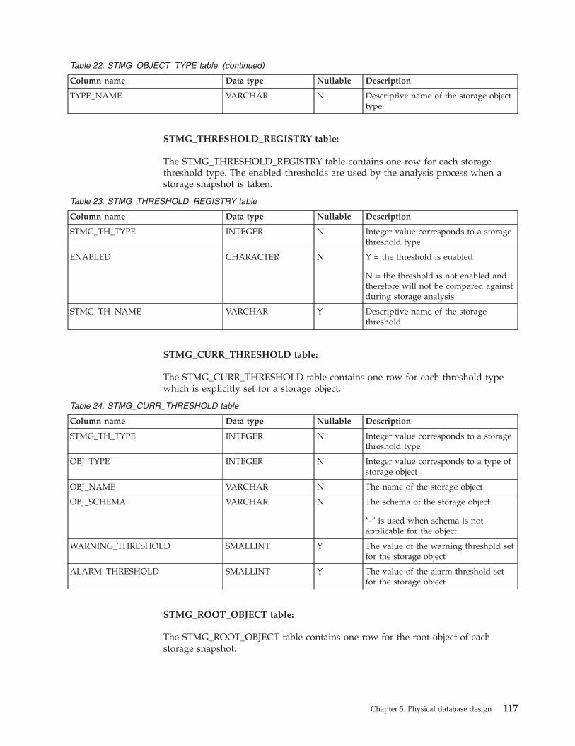
Table
22.
STMG_OBJECT_TYPE
table
(continued)
Column
name
Data
type
Nullable
Description
TYPE_NAME
VARCHAR
N
Descriptive
name
of
the
storage
object
type
STMG_THRESHOLD_REGISTRY
table:
The
STMG_THRESHOLD_REGISTRY
table
contains
one
row
for
each
storage
threshold
type.
The
enabled
thresholds
are
used
by
the
analysis
process
when
a
storage
snapshot
is
taken.
Table
23.
STMG_THRESHOLD_REGISTRY
table
Column
name
Data
type
Nullable
Description
STMG_TH_TYPE
INTEGER
N
Integer
value
corresponds
to
a
storage
threshold
type
ENABLED
CHARACTER
N
Y
=
the
threshold
is
enabled
N
=
the
threshold
is
not
enabled
and
therefore
will
not
be
compared
against
during
storage
analysis
STMG_TH_NAME
VARCHAR
Y
Descriptive
name
of
the
storage
threshold
STMG_CURR_THRESHOLD
table:
The
STMG_CURR_THRESHOLD
table
contains
one
row
for
each
threshold
type
which
is
explicitly
set
for
a
storage
object.
Table
24.
STMG_CURR_THRESHOLD
table
Column
name
Data
type
Nullable
Description
STMG_TH_TYPE
INTEGER
N
Integer
value
corresponds
to
a
storage
threshold
type
OBJ_TYPE
INTEGER
N
Integer
value
corresponds
to
a
type
of
storage
object
OBJ_NAME
VARCHAR
N
The
name
of
the
storage
object
OBJ_SCHEMA
VARCHAR
N
The
schema
of
the
storage
object.
″-″
is
used
when
schema
is
not
applicable
for
the
object
WARNING_THRESHOLD
SMALLINT
Y
The
value
of
the
warning
threshold
set
for
the
storage
object
ALARM_THRESHOLD
SMALLINT
Y
The
value
of
the
alarm
threshold
set
for
the
storage
object
STMG_ROOT_OBJECT
table:
The
STMG_ROOT_OBJECT
table
contains
one
row
for
the
root
object
of
each
storage
snapshot.
Chapter
5.
Physical
database
design
117

Table
25.
STMG_ROOT_OBJECT
table
Column
name
Data
type
Nullable
Description
STMG_TIMESTAMP
TIMESTAMP
N
The
timestamp
of
the
storage
snapshot.
It
indicates
when
the
data
capturing
process
started.
OBJ_TYPE
INTEGER
N
Integer
value
corresponds
to
a
type
of
storage
object
ROOT_ID
VARCHAR
N
The
ID
of
the
root
object
STMG_OBJECT
table:
The
STMG_OBJECT
table
contains
one
row
for
each
storage
object
that
is
analyzed
by
the
storage
snapshots
taken
so
far.
Table
26.
STMG_OBJECT
table
Column
name
Data
type
Nullable
Description
STMG_TIMESTAMP
TIMESTAMP
N
The
timestamp
of
the
storage
snapshot.
It
indicates
the
time
the
data
capturing
process
started.
ROOT_ID
CHARACTER
N
The
ID
of
the
root
object
OBJ_TYPE
INTEGER
N
Integer
value
corresponds
to
a
type
of
storage
object
OBJ_SCHEMA
VARCHAR
N
The
schema
of
the
storage
object.
″-″
is
used
when
schema
is
not
applicable
for
the
object
OBJ_NAME
VARCHAR
N
The
name
of
the
storage
object
DBPG_NAME
VARCHAR
Y
The
name
of
the
database
partition
group
the
object
residing
in.
Null
if
not
applicable.
TS_NAME
VARCHAR
Y
The
name
of
the
table
space
the
object
residing
in.
Null
if
not
applicable.
OBJ_ID
VARCHAR
N
The
unique
identifier
for
each
storage
object
under
a
given
storage
snapshot
timestamp
STMG_HIST_THRESHOLD
table:
The
STMG_HIST_THRESHOLD
table
contains
one
row
for
each
threshold
used
for
the
analyzing
the
storage
objects
at
the
time
the
storage
snapshots
are
taken.
Table
27.
STMG_HIST_THRESHOLD
table
Column
name
Data
type
Nullable
Description
STMG_TIMESTAMP
TIMESTAMP
N
The
timestamp
of
the
storage
snapshot.
It
indicates
the
time
the
data
capturing
process
started.
STMG_TH_TYPE
INTEGER
N
Integer
value
corresponds
to
a
storage
threshold
type
OBJ_ID
VARCHAR
N
The
unique
identifier
for
each
storage
object
under
a
given
storage
snapshot
timestamp
118
Administration
Guide:
Planning

Table
27.
STMG_HIST_THRESHOLD
table
(continued)
Column
name
Data
type
Nullable
Description
WARNING_THRESHOLD
SMALLINT
Y
The
value
of
the
warning
threshold
set
for
the
storage
object
at
the
time
the
storage
snapshot
was
taken.
ALARM_THRESHOLD
SMALLINT
Y
The
value
of
the
alarm
threshold
set
for
the
storage
object
at
the
time
the
storage
snapshot
was
taken
STMG_DATABASE
table:
The
STMG_DATABASE
table
contains
one
row
for
each
detailed
entry
of
database
storage
snapshots.
Table
28.
STMG_DATABASE
table
Column
name
Data
type
Nullable
Description
STMG_TIMESTAMP
TIMESTAMP
N
The
timestamp
of
the
storage
snapshot.
It
indicates
when
the
data
capturing
process
started.
OBJ_ID
VARCHAR
N
The
unique
identifier
for
each
storage
object
under
a
given
storage
snapshot
timestamp
COMPLETE_TIMESTAMP
TIMESTAMP
Y
The
timestamp
of
when
the
data
capturing
process
has
completed
for
the
database,
identified
by
OBJ_ID
column.
SPACE_THRESHOLD_EXCEEDED
SMALLINT
Y
A
flag
indicating
the
storage
space
usage
state
of
the
database.
0
=
normal
operational
state;
1
=
warning
threshold
exceeded;
2
=
alarm
threshold
exceeded.
SKEW_THRESHOLD_EXCEEDED
SMALLINT
Y
A
flag
indicating
the
data
distribution
state
of
the
database.
0
=
normal
operational
state;
1
=
warning
threshold
exceeded;
2
=
alarm
threshold
exceeded.
CR_THRESHOLD_EXCEEDED
SMALLINT
Y
A
flag
indicating
the
index
clustering
state
of
the
database.
0
=
normal
operational
state;
1
=
warning
threshold
exceeded;
2
=
alarm
threshold
exceeded.
STMG_DBPGROUP
table:
The
STMG_DBPGROUP
table
contains
one
row
for
each
detailed
entry
of
database
partition
group
storage
snapshots.
Chapter
5.
Physical
database
design
119

Table
29.
STMG_DBPGROUP
table
Column
name
Data
type
Nullable
Description
STMG_TIMESTAMP
TIMESTAMP
N
The
timestamp
of
the
storage
snapshot.
It
indicates
when
the
data
capturing
process
started.
OBJ_ID
VARCHAR
N
The
unique
identifier
for
each
storage
object
under
a
given
storage
snapshot
timestamp
COMPLETE_TIMESTAMP
TIMESTAMP
Y
The
timestamp
of
when
the
data
capturing
process
has
completed
for
the
database
partition
group,
identified
by
OBJ_ID
column.
SPACE_THRESHOLD_EXCEEDED
SMALLINT
Y
A
flag
indicating
the
storage
space
usage
state
of
the
database
partition
group.
0
=
normal
operational
state;
1
=
warning
threshold
exceeded;
2
=
alarm
threshold
exceeded.
SKEW_THRESHOLD_EXCEEDED
SMALLINT
Y
A
flag
indicating
the
data
distribution
state
of
the
database
partition
group.
0
=
normal
operational
state;
1
=
warning
threshold
exceeded;
2
=
alarm
threshold
exceeded.
PARTITON_COUNT
SMALLINT
Y
The
number
of
partitions
included
in
the
database
partition
group.
TARGET_LEVEL
BIGINT
Y
The
average
data
size,
in
bytes,
over
all
the
partitions
contained
by
the
database
partition
group.
It
is
the
target
level
of
even
data
distribution.
DATA_SKEW
SMALLINT
Y
A
percentage
of
the
maximum
data
size
deviation
from
the
TARGET_LEVEL
among
all
the
partitions.
This
value
is
used
during
data
capture
and
analysis
process
to
be
compared
against
the
data
distribution
skew
set
for
the
database
partition
group
in
the
STMG_CURR_THRESHOLD
table.
TOTAL_SIZE
BIGINT
Y
The
total
size,
in
bytes,
over
all
the
partitions
contained
by
the
database
partition
group.
It
is
the
sum
of
the
total
size
(number
of
pages
multiplied
by
page
size)
of
all
table
spaces
defined
under
the
database
partition
group.
For
DMS
table
spaces,
the
total
size
is
the
allocated
size;
for
SMS
table
spaces,
it
is
the
size
of
the
currently
used
by
the
table
space.
120
Administration
Guide:
Planning

Table
29.
STMG_DBPGROUP
table
(continued)
Column
name
Data
type
Nullable
Description
DATA_SIZE
BIGINT
Y
The
data
size,
in
bytes,
over
all
the
partitions
contained
by
the
database
partition
group.
It
is
the
sum
of
the
data
size
(number
of
data
pages
multiplied
by
page
size)
of
all
table
spaces
defined
under
the
database
partition
group.
PERCENT_USED
SMALLINT
Y
A
percentage
value
of
data
size
over
total
size.
This
value
is
compared
against
the
space
usage
threshold
during
the
data
capture
and
analysis
process.
In
the
case
of
SMS
table
spaces,
the
space
usage
threshold
for
the
table
space
or
its
parent
database
partition
group
should
be
set
to
100
to
avoid
unnecessary
alarms.
STMG_DBPARTITION
table:
The
STMG_DBPARTITION
table
contains
one
row
for
each
detailed
entry
of
database
partition
storage
snapshots.
This
is
meant
to
be
used
along
with
the
STMG_DBPGROUP
table.
Table
30.
STMG_DBPARTITION
table
Column
name
Data
type
Nullable
Description
STMG_TIMESTAMP
TIMESTAMP
N
The
timestamp
of
the
storage
snapshot.
It
indicates
when
the
data
capturing
process
started.
OBJ_ID
VARCHAR
N
The
unique
identifier
for
each
storage
object
under
a
given
storage
snapshot
timestamp
PARTITION_NUM
INTEGER
Y
The
database
partition
number.
COMPLETE_TIMESTAMP
TIMESTAMP
Y
The
timestamp
of
when
the
data
capturing
process
has
completed
for
the
database
partition,
identified
by
OBJ_ID
column.
DBPG_NAME
CHARACTER
Y
The
name
of
database
partition
group
IN_USE
CHARACTER
Y
Status
of
the
partition
at
the
time
of
the
storage
snapshot.
Same
as
IN_USE
column
in
SYSCAT.NODEGROUPDEF.
HOST_NAME
VARCHAR
Y
The
host
name
of
the
database
partition.
HOST_SYSTEM_SIZE
BIGINT
Y
NOT
AVAILABLE
EST_DATA_SIZE
BIGINT
Y
The
estimated
data
size
on
the
database
partition,
within
the
database
partition
group
scope.
This
value
is
calculated
as
the
sum
of
the
table
partition
data
size,
for
the
given
partition.
STMG_TABLESPACE
table:
Chapter
5.
Physical
database
design
121

The
STMG_TABLESPACE
table
contains
one
row
for
each
detailed
entry
of
table
space
storage
snapshots.
Table
31.
STMG_TABLESPACE
table
Column
name
Data
type
Nullable
Description
STMG_TIMESTAMP
TIMESTAMP
N
The
timestamp
of
the
storage
snapshot.
It
indicates
when
the
data
capturing
process
started.
OBJ_ID
VARCHAR
N
The
unique
identifier
for
each
storage
object
under
a
given
storage
snapshot
timestamp
COMPLETE_TIMESTAMP
TIMESTAMP
Y
The
timestamp
of
when
the
data
capturing
process
has
completed
for
the
table
space,
identified
by
OBJ_ID
column.
SPACE_THRESHOLD_EXCEEDED
SMALLINT
Y
A
flag
indicating
the
storage
space
usage
state
of
the
table
space.
0
=
normal
operational
state;
1
=
warning
threshold
exceeded;
2
=
alarm
threshold
exceeded
TYPE
CHARACTER
Y
As
defined
in
SYSCAT.TABLESPACES
DATATYPE
CHARACTER
Y
As
defined
in
SYSCAT.TABLESPACES
TOTAL_SIZE
BIGINT
Y
As
defined
in
SYSCAT.TABLESPACES
PERCENT_USED
SMALLINT
Y
As
defined
in
SYSCAT.TABLESPACES.
This
is
used
during
data
capture
and
analysis
process
to
be
compared
against
the
space
usage
threshold
in
the
STMG_CURR_THRESHOLD
table.
DATA_SIZE
BIGINT
Y
As
defined
in
SYSCAT.TABLESPACES
DATA_PAGE
BIGINT
Y
As
defined
in
SYSCAT.TABLESPACES
EXTENT_SIZE
INTEGER
Y
As
defined
in
SYSCAT.TABLESPACES
PREFETCH_SIZE
INTEGER
Y
As
defined
in
SYSCAT.TABLESPACES
OVERHEAD
DOUBLE
Y
As
defined
in
SYSCAT.TABLESPACES
TRANSFER_RATE
DOUBLE
Y
As
defined
in
SYSCAT.TABLESPACES
BUFFERPOOL_ID
INTEGER
Y
As
defined
in
SYSCAT.TABLESPACES
PAGE_SIZE
INTEGER
Y
As
defined
in
SYSCAT.TABLESPACES
STMG_CONTAINER
table:
The
STMG_CONTAINER
table
contains
one
row
for
each
detailed
entry
of
container
storage
snapshots.
Table
32.
STMG_CONTAINER
table
Column
name
Data
type
Nullable
Description
STMG_TIMESTAMP
TIMESTAMP
N
The
timestamp
of
the
storage
snapshot.
It
indicates
when
the
data
capturing
process
started.
OBJ_ID
VARCHAR
N
The
unique
identifier
for
each
storage
object
under
a
given
storage
snapshot
timestamp
122
Administration
Guide:
Planning

Table
32.
STMG_CONTAINER
table
(continued)
Column
name
Data
type
Nullable
Description
COMPLETE_TIMESTAMP
TIMESTAMP
Y
The
timestamp
of
when
the
data
capturing
process
has
completed
for
the
container,
identified
by
OBJ_ID
column.
TS_ID
INTEGER
Y
The
integer
ID
for
the
table
space
which
the
container
is
assigned
to.
SPACE_THRESHOLD_EXCEEDED
SMALLINT
Y
A
flag
indicating
the
storage
space
usage
state
of
the
container.
0
=
normal
operational
state;
1
=
warning
threshold
exceeded;
2
=
alarm
threshold
exceeded.
PARTITION_NUM
INTEGER
Y
The
partition
number
of
the
database
partition
where
the
container
resides.
TYPE
CHARACTER
Y
’P’
=
path
container;
’F’
=
file
container;
’D’
=
raw
device
container
TOTAL_PAGE
BIGINT
Y
Total
pages
allocated
for
the
container.
USABLE_PAGES
BIGINT
Y
Number
of
usable
pages
in
the
container.
PERCENT_USED
SMALLINT
Y
NOT
AVAILABLE.
This
is
to
be
used
during
data
capture
and
analysis
process
to
be
compared
against
the
space
usage
threshold
in
the
STMG_CURR_THRESHOLD
table.
DATA_SIZE
BIGINT
Y
NOT
AVAILABLE
DATA_PAGE
BIGINT
Y
NOT
AVAILABLE
STMG_TABLE
table:
The
STMG_TABLE
table
contains
one
row
for
each
detailed
entry
of
table
storage
snapshots.
Table
33.
STMG_TABLE
table
Column
name
Data
type
Nullable
Description
STMG_TIMESTAMP
TIMESTAMP
N
The
timestamp
of
the
storage
snapshot.
It
indicates
when
the
data
capturing
process
started.
OBJ_ID
VARCHAR
N
The
unique
identifier
for
each
storage
object
under
a
given
storage
snapshot
timestamp
COMPLETE_TIMESTAMP
TIMESTAMP
Y
The
timestamp
of
when
the
data
capturing
process
has
completed
for
the
table,
identified
by
OBJ_ID
column.
DBPG_NAME
VARCHAR
Y
The
name
of
the
database
partition
group
the
table
resides
in.
Chapter
5.
Physical
database
design
123

Table
33.
STMG_TABLE
table
(continued)
Column
name
Data
type
Nullable
Description
SKEW_THRESHOLD_EXCEEDED
SMALLINT
Y
A
flag
indicating
the
data
distribution
state
of
the
table.
0
=
normal
operational
state;
1
=
warning
threshold
exceeded;
2
=
alarm
threshold
exceeded.
TOTAL_ROW_COUNT
BIGINT
Y
Total
row
count
of
the
table
AVG_ROW_COUNT
BIGINT
Y
The
average
row
count
over
all
the
table
partitions
TARGET_LEVEL
BIGINT
Y
The
average
data
size
on
each
partition,
in
bytes
DATA_SKEW
SMALLINT
Y
The
maximum
percentage
of
the
ROW_COUNT
value
deviated
from
the
TARGET_LEVEL,
over
all
table
partitions,
for
the
given
table.
This
is
used
during
data
capture
and
analysis
process
to
be
compared
against
the
data
skew
threshold
in
the
STMG_CURR_THRESHOLD
table.
AVG_ROW_LENGTH
BIGINT
Y
The
average
row
length
of
the
table.
If
this
statistic
has
been
collected,
it
will
be
the
sum
of
the
average
column
length
of
all
the
columns
in
this
table;
when
there
is
no
statistical
data,
this
value
is
calculated
by
adding
the
fixed
columns’
length
with
the
percentage
of
the
variable
columns’
length.
COLCOUNT
INTEGER
Y
As
defined
in
SYSCAT.TABLES
ESTIMATED_SIZE
BIGINT
Y
As
defined
in
SYSCAT.TABLES
NPAGES
INTEGER
Y
As
defined
in
SYSCAT.TABLES
FPAGES
INTEGER
Y
As
defined
in
SYSCAT.TABLES
OVERFLOW
INTEGER
Y
As
defined
in
SYSCAT.TABLES
MAIN_TBSPACE
VARCHAR
Y
As
defined
in
SYSCAT.TABLES
INDEX_TBSPACE
VARCHAR
Y
As
defined
in
SYSCAT.TABLES
LONG_TBSPACE
VARCHAR
Y
As
defined
in
SYSCAT.TABLES
STMG_TBPARTITION
table:
The
STMG_TBPARTITION
table
contains
one
row
for
each
detailed
entry
of
table
partition
storage
snapshots.
Table
34.
STMG_TBPARTITION
table
Column
name
Data
type
Nullable
Description
STMG_TIMESTAMP
TIMESTAMP
N
The
timestamp
of
the
storage
snapshot.
It
indicates
when
the
data
capturing
process
started.
OBJ_ID
VARCHAR
N
The
unique
identifier
for
each
storage
object
under
a
given
storage
snapshot
timestamp
124
Administration
Guide:
Planning

Table
34.
STMG_TBPARTITION
table
(continued)
Column
name
Data
type
Nullable
Description
PARTITION_NUM
INTEGER
N
The
partition
number
of
the
database
partition
where
the
table
partition
resides.
COMPLETE_TIMESTAMP
TIMESTAMP
Y
The
timestamp
of
when
the
data
capturing
process
has
completed
for
the
table
partition,
identified
by
OBJ_ID
column.
DBPG_NAME
VARCHAR
Y
The
name
of
the
database
partition
group
where
the
table
resides.
ROWCOUNT
BIGINT
Y
The
number
of
rows
in
this
table
partition
STMG_INDEX
table:
The
STMG_INDEX
table
contains
one
row
for
each
detailed
entry
of
index
storage
snapshots.
Table
35.
STMG_INDEX
table
Column
name
Data
type
Nullable
Description
STMG_TIMESTAMP
TIMESTAMP
N
The
timestamp
of
the
storage
snapshot.
It
indicates
when
the
data
capturing
process
started.
OBJ_ID
VARCHAR
N
The
unique
identifier
for
each
storage
object
under
a
given
storage
snapshot
timestamp
COMPLETE_TIMESTAMP
TIMESTAMP
Y
The
timestamp
of
when
the
data
capturing
process
has
completed
for
the
index,
identified
by
OBJ_ID
column.
DBPG_NAME
VARCHAR
Y
The
name
of
the
database
partition
group
where
the
index
resides
in.
TB_SCHEMA
VARCHAR
Y
As
TABNAME
defined
in
SYSCAT.INDEXES
TB_NAME
VARCHAR
Y
As
TABSCHEMA
defined
in
SYSCAT.INDEXES
CR_THRESHOLD_EXCEEDED
SMALLINT
Y
A
flag
indicating
the
index
clustering
state.
0
=
normal
operational
state;
1
=
warning
threshold
exceeded;
2
=
alarm
threshold
exceeded.
COLCOUNT
INTEGER
Y
As
defined
in
SYSCAT.INDEXES
ESTIMATED_SIZE
BIGINT
Y
As
defined
in
SYSCAT.INDEXES
NLEAF
INTEGER
Y
As
defined
in
SYSCAT.INDEXES
NLEVELS
SMALLINT
Y
As
defined
in
SYSCAT.INDEXES
FIRSTKEYCARD
BIGINT
Y
As
defined
in
SYSCAT.INDEXES
FIRST2KEYCARD
BIGINT
Y
As
defined
in
SYSCAT.INDEXES
FIRST3KEYCARD
BIGINT
Y
As
defined
in
SYSCAT.INDEXES
Chapter
5.
Physical
database
design
125

Table
35.
STMG_INDEX
table
(continued)
Column
name
Data
type
Nullable
Description
FIRST4KEYCARD
BIGINT
Y
As
defined
in
SYSCAT.INDEXES
FULLKEYCARD
BIGINT
Y
As
defined
in
SYSCAT.INDEXES
CLUSTERRATIO
SMALLINT
Y
As
defined
in
SYSCAT.INDEXES,
this
is
used
during
data
capture
and
analysis
process
to
compare
against
the
threshold
set
for
the
given
index.
CLUSTERFACTOR
BIGINT
Y
As
defined
in
SYSCAT.INDEXES
SEQUENTIAL_PAGES
INTEGER
Y
As
defined
in
SYSCAT.INDEXES
DENSITY
INTEGER
Y
As
defined
in
SYSCAT.INDEXES
Related
reference:
v
“Storage
management
view”
on
page
115
Temporary
table
space
design
It
is
recommended
that
you
define
a
single
SMS
temporary
table
space
with
a
page
size
equal
to
the
page
size
used
in
the
majority
of
your
regular
table
spaces.
This
should
be
suitable
for
typical
environments
and
workloads.
However,
it
can
be
advantageous
to
experiment
with
different
temporary
table
space
configurations
and
workloads.
The
following
points
should
be
considered:
v
Temporary
tables
are
in
most
cases
accessed
in
batches
and
sequentially.
That
is,
a
batch
of
rows
is
inserted,
or
a
batch
of
sequential
rows
is
fetched.
Therefore,
a
larger
page
size
typically
results
in
better
performance,
because
fewer
logical
or
physical
page
I/O
requests
are
required
to
read
a
given
amount
of
data.
This
is
not
always
the
case
when
the
average
temporary
table
row
size
is
smaller
than
the
page
size
divided
by
255.
A
maximum
of
255
rows
can
exist
on
any
page,
regardless
of
the
page
size.
For
example,
a
query
that
requires
a
temporary
table
with
15-byte
rows
would
be
better
served
by
a
4
KB
temporary
table
space
page
size,
because
255
such
rows
can
all
be
contained
within
a
4
KB
page.
An
8
KB
(or
larger)
page
size
would
result
in
at
least
4
KB
(or
more)
bytes
of
wasted
space
on
each
temporary
table
page,
and
would
not
reduce
the
number
of
required
I/O
requests.
v
If
more
than
fifty
percent
of
the
regular
table
spaces
in
your
database
use
the
same
page
size,
it
can
be
advantageous
to
define
your
temporary
table
spaces
with
the
same
page
size.
The
reason
for
this
is
that
this
arrangement
enables
your
temporary
table
space
to
share
the
same
buffer
pool
space
with
most
or
all
of
your
regular
table
spaces.
This,
in
turn,
simplifies
buffer
pool
tuning.
v
When
reorganizing
a
table
using
a
temporary
table
space,
the
page
size
of
the
temporary
table
space
must
match
that
of
the
table.
For
this
reason,
you
should
ensure
that
there
are
temporary
table
spaces
defined
for
each
different
page
size
used
by
existing
tables
that
you
may
reorganize
using
a
temporary
table
space.
You
can
also
reorganize
without
a
temporary
table
space
by
reorganizing
the
table
directly
in
the
target
table
space.
Of
course,
this
type
of
reorganization
requires
that
there
be
extra
space
in
the
target
table
space
for
the
reorganization
process.
v
If
you
are
reliant
on
system
temporary
tables
in
SMS
system
temporary
table
spaces
because
of
your
work
envionment,
you
may
want
to
consider
using
the
registry
variable
DB2_SMS_TRUNC_TMPTABLE_THRESH.
In
the
past
when
system
temporary
tables
were
no
longer
needed,
they
were
truncated
to
a
file
126
Administration
Guide:
Planning
||||

size
of
zero.
The
need
for
a
new
system
temporary
table
would
have
a
performance
cost
associated
with
it.
Using
this
registry
variable
allows
for
leaving
non-zero
system
temporary
tables
on
the
system
to
avoid
the
performance
cost
of
repeated
creations
and
truncations
of
system
temporary
tables.
v
In
general,
when
temporary
table
spaces
of
differing
page
sizes
exist,
the
optimizer
will
most
often
choose
the
temporary
table
space
with
the
largest
buffer
pool.
In
such
cases,
it
is
often
wise
to
assign
an
ample
buffer
pool
to
one
of
the
temporary
table
spaces,
and
leave
any
others
with
a
smaller
buffer
pool.
Such
a
buffer
pool
assignment
will
help
ensure
efficient
utilization
of
main
memory.
For
example,
if
your
catalog
table
space
uses
4
KB
pages,
and
the
remaining
table
spaces
use
8
KB
pages,
the
best
temporary
table
space
configuration
may
be
a
single
8
KB
temporary
table
space
with
a
large
buffer
pool,
and
a
single
4
KB
table
space
with
a
small
buffer
pool.
Note:
Catalog
table
spaces
are
restricted
to
using
the
4
KB
page
size.
As
such,
the
database
manager
always
enforces
the
existence
of
a
4
KB
system
temporary
table
space
to
enable
catalog
table
reorganizations.
v
There
is
generally
no
advantage
to
defining
more
than
one
temporary
table
space
of
any
single
page
size.
v
SMS
is
almost
always
a
better
choice
than
DMS
for
temporary
table
spaces
because:
–
There
is
more
overhead
in
the
creation
of
a
temporary
table
when
using
DMS
versus
SMS.
–
Disk
space
is
allocated
on
demand
in
SMS,
whereas
it
must
be
pre-allocated
in
DMS.
Pre-allocation
can
be
difficult:
Temporary
table
spaces
hold
transient
data
that
can
have
a
very
large
peak
storage
requirement,
and
a
much
smaller
average
storage
requirement.
With
DMS,
the
peak
storage
requirement
must
be
pre-allocated,
whereas
with
SMS,
the
extra
disk
space
can
be
used
for
other
purposes
during
off-peak
hours.
–
The
database
manager
attempts
to
keep
temporary
table
pages
in
memory,
rather
than
writing
them
out
to
disk.
As
a
result,
the
performance
advantages
of
DMS
are
less
significant.
Related
concepts:
v
“Table
space
design”
on
page
89
v
“System
managed
space”
on
page
92
v
“Temporary
tables
in
SMS
table
spaces”
on
page
127
Related
reference:
v
“REORG
INDEXES/TABLE
Command”
in
the
Command
Reference
Temporary
tables
in
SMS
table
spaces
Temporary
tables
in
SMS
table
spaces
are
not
deleted
by
default
once
they
are
no
longer
needed.
Instead,
files
associated
with
temporary
tables
that
are
larger
than
one
extent
in
size
are
truncated
to
one
extent.
In
cases
where
temporary
tables
are
used
repeatedly,
this
avoids
some
of
the
performance
cost
of
deleting
and
recreating
temporary
tables.
This
reuse
of
temporary
tables
benefits
users
whose
workload
involves
dealing
with
many
small
temporary
tables
on
smaller
systems
such
as
Windows®
NT
Chapter
5.
Physical
database
design
127
|||||
|
|||||
||

where
the
file
system
calls
are
relatively
expensive;
and
users
whose
disk
storage
is
distributed,
requiring
network
messages
to
complete
file
system
operations.
By
default,
files
that
hold
temporary
tables
larger
than
one
extent
are
truncated
to
one
extent
once
they
are
no
longer
needed.
You
can
increase
this
amount
by
specifying
a
larger
value
for
the
DB2®_SMS_TRUNC_TMPTABLE_THRESH
registry
variable.
You
should
increase
the
value
associated
with
this
registry
variable
if
your
workload
repeatedly
uses
large
SMS
temporary
tables
and
you
can
afford
to
leave
space
allocated
between
uses.
You
can
turn
off
this
feature
by
specifying
a
value
of
0
for
the
DB2_SMS_TRUNC_TMPTABLE_THRESH
registry
variable.
You
might
want
to
do
this
if
your
system
has
restrictive
space
limitations
and
you
are
experiencing
repeated
out
of
disk
errors
for
SMS
temporary
table
spaces.
The
first
connection
to
the
database
deletes
any
previously
allocated
files.
If
you
want
to
clear
out
existing
temporary
tables,
you
should
drop
all
database
connections
and
reconnect,
or
deactivate
the
database
and
reactivate
it.
If
you
want
to
ensure
that
space
for
temporary
tables
stays
allocated,
use
the
ACTIVATE
DATABASE
command
to
start
the
database.
This
will
avoid
the
repeated
cost
of
startup
on
the
first
connect
to
the
database.
Related
concepts:
v
“Temporary
table
space
design”
on
page
126
Catalog
table
space
design
An
SMS
table
space
is
recommended
for
database
catalogs,
for
the
following
reasons:
v
The
database
catalog
consists
of
many
tables
of
varying
sizes.
When
using
a
DMS
table
space,
a
minimum
of
two
extents
are
allocated
for
each
table
object.
Depending
on
the
extent
size
chosen,
a
significant
amount
of
allocated
and
unused
space
may
result.
When
using
a
DMS
table
space,
a
small
extent
size
(two
to
four
pages)
should
be
chosen;
otherwise,
an
SMS
table
space
should
be
used.
v
There
are
large
object
(LOB)
columns
in
the
catalog
tables.
LOB
data
is
not
kept
in
the
buffer
pool
with
other
data,
but
is
read
from
disk
each
time
it
is
needed.
Reading
LOBs
from
disk
reduces
performance.
Since
a
file
system
usually
has
its
own
cache,
using
an
SMS
table
space,
or
a
DMS
table
space
built
on
file
containers,
makes
avoidance
of
I/O
possible
if
the
LOB
has
previously
been
referenced.
Given
these
considerations,
an
SMS
table
space
is
a
somewhat
better
choice
for
the
catalogs.
Another
factor
to
consider
is
whether
you
will
need
to
enlarge
the
catalog
table
space
in
the
future.
While
some
platforms
have
support
for
enlarging
the
underlying
storage
for
SMS
containers,
and
while
you
can
use
redirected
restore
to
enlarge
an
SMS
table
space,
the
use
of
a
DMS
table
space
facilitates
the
addition
of
new
containers.
Related
concepts:
v
“Definition
of
system
catalog
tables”
in
the
Administration
Guide:
Implementation
v
“Table
space
design”
on
page
89
128
Administration
Guide:
Planning
||
||||||
||||
||||||
|
|

v
“System
managed
space”
on
page
92
v
“Database
managed
space”
on
page
94
Optimizing
table
space
performance
when
data
is
on
RAID
devices
This
section
describes
how
to
optimize
performance
when
data
is
placed
on
Redundant
Array
of
Independent
Disks
(RAID)
devices.
Procedure:
You
should
do
the
following
for
each
table
space
that
uses
a
RAID
device:
v
Define
a
single
container
for
the
table
space
(using
the
RAID
device).
v
Make
the
EXTENTSIZE
of
the
table
space
equal
to,
or
a
multiple
of,
the
RAID
stripe
size.
v
Ensure
that
the
PREFETCHSIZE
of
the
table
space
is:
–
the
RAID
stripe
size
multiplied
by
the
number
of
RAID
parallel
devices
(or
a
whole
multiple
of
this
product),
and
–
a
multiple
of
the
EXTENTSIZE.v
Use
the
DB2_PARALLEL_IO
registry
variable
to
enable
parallel
I/O
for
the
table
space.
DB2_PARALLEL_IO:
When
reading
data
from,
or
writing
data
to
table
space
containers,
DB2
Universal
Database™
(DB2
UDB)
may
use
parallel
I/O
if
the
number
of
containers
in
the
database
is
greater
than
1.
However,
there
are
situations
when
it
would
be
beneficial
to
have
parallel
I/O
enabled
for
single
container
table
spaces.
For
example,
if
the
container
is
created
on
a
single
RAID
device
that
is
composed
of
more
than
one
physical
disk,
you
may
want
to
issue
parallel
read
and
write
calls.
To
force
parallel
I/O
for
a
table
space
that
has
a
single
container,
you
can
use
the
DB2_PARALLEL_IO
registry
variable.
This
variable
can
be
set
to
″*″
(asterisk),
meaning
every
table
space,
or
it
can
be
set
to
a
list
of
table
space
IDs
separated
by
commas.
For
example:
db2set
DB2_PARALLEL_IO=*
{turn
parallel
I/O
on
for
all
table
spaces}
db2set
DB2_PARALLEL_IO=1,2,4,8
{turn
parallel
I/O
on
for
table
spaces
1,
2,
4,
and
8}
After
setting
the
registry
variable,
DB2
UDB
must
be
stopped
(db2stop),
and
then
restarted
(db2start),
for
the
changes
to
take
effect.
DB2_PARALLEL_IO
also
affects
table
spaces
with
more
than
one
container
defined.
If
you
do
not
set
the
registry
variable,
the
I/O
parallelism
is
equal
to
the
number
of
containers
in
the
table
space.
If
you
set
the
registry
variable,
the
I/O
parallelism
is
equal
to
the
result
of
prefetch
size
divided
by
extent
size.
You
might
want
to
set
the
registry
variable
if
the
individual
containers
in
the
table
space
are
striped
across
multiple
physical
disks.
For
example,
a
table
space
has
two
containers
and
the
prefetch
size
is
four
times
the
extent
size.
If
the
registry
variable
is
not
set,
a
prefetch
request
for
this
table
space
will
be
broken
into
two
requests
(each
request
will
be
for
two
extents).
Provided
that
the
prefetchers
are
available
to
do
work,
two
prefetchers
can
be
working
on
these
requests
in
parallel.
In
the
case
where
the
registry
variable
is
set,
Chapter
5.
Physical
database
design
129
||||||

a
prefetch
request
for
this
table
space
will
be
broken
into
four
requests
(one
extent
per
request)
with
a
possibility
of
four
prefetchers
servicing
the
requests
in
parallel.
In
this
example,
if
each
of
the
two
containers
had
a
single
disk
dedicated
to
it,
setting
the
registry
variable
for
this
table
space
might
result
in
contention
on
those
disks
since
two
prefetchers
will
be
accessing
each
of
the
two
disks
at
once.
However,
if
each
of
the
two
containers
was
striped
across
multiple
disks,
setting
the
registry
variable
would
potentially
allow
access
to
four
different
disks
at
once.
DB2_USE_PAGE_CONTAINER_TAG:
By
default,
DB2
UDB
uses
the
first
extent
of
each
DMS
container
(file
or
device)
to
store
a
container
tag.
The
container
tag
is
DB2
UDB’s
metadata
for
the
container.
In
earlier
versions
of
DB2
UDB,
the
first
page
was
used
for
the
container
tag,
instead
of
the
first
extent,
and
as
a
result
less
space
in
the
container
was
used
to
store
the
tag.
(In
earlier
versions
of
DB2
UDB,
the
DB2_STRIPED_CONTAINERS
registry
variable
was
used
to
create
table
spaces
with
an
extent
sized
tag.
However,
because
this
is
now
the
default
behavior,
this
registry
variable
no
longer
has
any
affect.)
When
the
DB2_USE_PAGE_CONTAINER_TAG
registry
variable
is
set
to
ON,
any
new
DMS
containers
created
will
be
created
with
a
one-page
tag,
instead
of
a
one-extent
tag
(the
default).
There
will
be
no
impact
to
existing
containers
that
were
created
before
the
registry
variable
was
set.
Setting
this
registry
variable
to
ON
is
not
recommended
unless
you
have
very
tight
space
constraints,
or
you
require
behavior
consistent
with
pre-Version
8
databases.
Setting
this
registry
variable
to
ON
can
have
a
negative
impact
on
I/O
performance
if
RAID
devices
are
used
for
table
space
containers.
When
using
RAID
devices
for
table
space
containers,
it
is
suggested
that
the
table
space
be
created
with
an
extent
size
that
is
equal
to,
or
a
multiple
of,
the
RAID
stripe
size.
However,
if
this
registry
variable
is
set
to
ON,
a
one-page
container
tag
will
be
used
and
the
extents
will
not
line
up
with
the
RAID
stripes.
As
a
result
it
may
be
necessary
during
an
I/O
request
to
access
more
physical
disks
than
would
be
optimal.
Users
are
thus
strongly
advised
against
setting
this
registry
variable.
To
create
containers
with
one-page
container
tags,
set
this
registry
variable
to
ON,
and
then
stop
and
restart
the
instance:
db2set
DB2_USE_PAGE_CONTAINER_TAG=ON
db2stop
db2start
To
stop
creating
containers
with
one-page
container
tags,
reset
this
registry
variable,
and
then
stop
and
restart
the
instance.
db2set
DB2_USE_PAGE_CONTAINER_TAG=
db2stop
db2start
The
Control
Center,
the
LIST
TABLESPACE
CONTAINERS
command,
and
the
GET
SNAPSHOT
FOR
TABLESPACES
command
do
not
show
whether
a
container
has
been
created
with
a
page
or
extent
sized
tag.
They
use
the
label
“file”
or
“device,”
depending
on
how
the
container
was
created.
To
verify
whether
a
container
was
created
with
a
page-
or
extent-size
tag,
you
can
use
the
/DTSF
option
of
DB2DART
to
dump
table
space
and
container
information,
and
then
look
at
the
130
Administration
Guide:
Planning

type
field
for
the
container
in
question.
The
query
container
APIs
(sqlbftcq
and
sqlbtcq),
can
be
used
to
create
a
simple
application
that
will
display
the
type.
Related
concepts:
v
“Table
space
design”
on
page
89
Related
reference:
v
“System
environment
variables”
in
the
Administration
Guide:
Performance
Considerations
when
choosing
table
spaces
for
your
tables
When
determining
how
to
map
tables
to
table
spaces,
you
should
consider:
v
The
partitioning
of
your
tables.
At
a
minimum,
you
should
ensure
that
the
table
space
you
choose
is
in
a
database
partition
group
with
the
partitioning
you
want.
v
The
amount
of
data
in
the
table.
If
you
plan
to
store
many
small
tables
in
a
table
space,
consider
using
SMS
for
that
table
space.
The
DMS
advantages
with
I/O
and
space
management
efficiency
are
not
as
important
with
small
tables.
The
SMS
advantages
of
allocating
space
one
page
at
a
time,
and
only
when
needed,
are
more
attractive
with
smaller
tables.
If
one
of
your
tables
is
larger,
or
you
need
faster
access
to
the
data
in
the
tables,
a
DMS
table
space
with
a
small
extent
size
should
be
considered.
You
may
wish
to
use
a
separate
table
space
for
each
very
large
table,
and
group
all
small
tables
together
in
a
single
table
space.
This
separation
also
allows
you
to
select
an
appropriate
extent
size
based
on
the
table
space
usage.
v
The
type
of
data
in
the
table.
You
may,
for
example,
have
tables
containing
historical
data
that
is
used
infrequently;
the
end-user
may
be
willing
to
accept
a
longer
response
time
for
queries
executed
against
this
data.
In
this
situation,
you
could
use
a
different
table
space
for
the
historical
tables,
and
assign
this
table
space
to
less
expensive
physical
devices
that
have
slower
access
rates.
Alternatively,
you
may
be
able
to
identify
some
essential
tables
for
which
the
data
has
to
be
readily
available
and
for
which
you
require
fast
response
time.
You
may
want
to
put
these
tables
into
a
table
space
assigned
to
a
fast
physical
device
that
can
help
support
these
important
data
requirements.
Using
DMS
table
spaces,
you
can
also
distribute
your
table
data
across
three
different
table
spaces:
one
for
index
data;
one
for
LOB
and
long
field
data;
and
one
for
regular
table
data.
This
allows
you
to
choose
the
table
space
characteristics
and
the
physical
devices
supporting
those
table
spaces
to
best
suit
the
data.
For
example,
you
could
put
your
index
data
on
the
fastest
devices
you
have
available,
and
as
a
result,
obtain
significant
performance
improvements.
If
you
split
a
table
across
DMS
table
spaces,
you
should
consider
backing
up
and
restoring
those
table
spaces
together
if
roll-forward
recovery
is
enabled.
SMS
table
spaces
do
not
support
this
type
of
data
distribution
across
table
spaces.
v
Administrative
issues.
Some
administrative
functions
can
be
performed
at
the
table
space
level
instead
of
the
database
or
table
level.
For
example,
taking
a
backup
of
a
table
space
instead
of
a
database
can
help
you
make
better
use
of
your
time
and
resources.
It
allows
you
to
frequently
back
up
table
spaces
with
large
volumes
of
changes,
while
only
occasionally
backing
up
tables
spaces
with
very
low
volumes
of
changes.
Chapter
5.
Physical
database
design
131

You
can
restore
a
database
or
a
table
space.
If
unrelated
tables
do
not
share
table
spaces,
you
have
the
option
to
restore
a
smaller
portion
of
your
database
and
reduce
costs.
A
good
approach
is
to
group
related
tables
in
a
set
of
table
spaces.
These
tables
could
be
related
through
referential
constraints,
or
through
other
defined
business
constraints.
If
you
need
to
drop
and
redefine
a
particular
table
often,
you
may
want
to
define
the
table
in
its
own
table
space,
because
it
is
more
efficient
to
drop
a
DMS
table
space
than
it
is
to
drop
a
table.
Related
concepts:
v
“Database
partition
groups”
on
page
81
v
“System
managed
space”
on
page
92
v
“Database
managed
space”
on
page
94
v
“Comparison
of
SMS
and
DMS
table
spaces”
on
page
109
Tables
used
within
DB2
UDB
DB2®
Universal
Database
(DB2
UDB)
provides
the
following
types
of
tables:
v
Regular
tables,
which
are
implemented
as
a
heap
v
Append
mode
tables,
which
are
regular
tables
that
are
optimized
primarily
for
INSERTs
v
Multidimensional
clustering
(MDC)
tables,
which
are
implemented
as
tables
that
are
physically
clustered
on
more
than
one
key,
or
dimension,
at
the
same
time
v
Range-clustered
tables
(RCT),
which
are
implemented
as
sequential
clusters
of
data
that
provide
fast,
direct
access
Each
type
of
table
has
characteristics
that
make
it
useful
when
working
in
a
particular
business
environment.
For
each
table
that
you
use,
consider
which
table
types
would
best
suit
your
needs.
Regular
tables
with
indexes
are
the
“general
purpose”
table
choice.
Regular
tables
are
placed
into
append
mode
through
an
ALTER
TABLE
statement.
Append
mode
tables
are
suitable
where
you
need
to
add
new
data
and
retrieve
existing
data
such
as
where
you
are
dealing
with
customer
accounts
in
a
banking
environment.
There
you
record
each
change
to
the
account
through
debits,
credits,
and
transfers.
You
also
have
customers
who
want
to
review
the
history
of
changes
to
that
account.
Multidimensional
clustering
tables
are
used
in
data
warehousing
and
large
database
environments.
Clustering
indexes
on
regular
tables
support
single-dimensional
clustering
of
data.
MDC
tables
provide
the
benefits
of
data
clustering
across
more
than
one
dimension.
Range-clustered
tables
are
used
where
the
data
is
tightly
clustered
across
one
or
more
columns
in
the
table.
The
largest
and
smallest
values
in
the
columns
define
the
range
of
possible
values.
You
use
these
columns
to
access
records
in
the
table.
Related
concepts:
v
“Multidimensional
clustering
tables”
on
page
137
v
“Range-clustered
tables”
on
page
133
132
Administration
Guide:
Planning
|
|
|
||
||
||
|||
|
||||||
||||
|||
|
|
|

Related
tasks:
v
“Creating
and
populating
a
table”
in
the
Administration
Guide:
Implementation
v
“Creating
a
materialized
query
table”
in
the
Administration
Guide:
Implementation
Range-clustered
tables
A
range-clustered
table
(RCT)
is
a
table
layout
scheme
where
each
record
in
the
table
has
a
predetermined
record
ID
(RID)
which
is
an
internal
identifier
used
to
locate
a
record
in
a
table.
For
each
table
that
holds
your
data,
consider
which
of
the
possible
table
types
would
best
suit
your
needs.
For
example,
if
you
have
data
records
that
will
be
loosely
clustered
(not
monotonically
increasing),
consider
using
a
regular
table
and
indexes.
If
you
have
data
records
that
will
have
duplicate
(not
unique)
values
in
the
key,
you
should
not
use
a
range-clustered
table.
If
you
cannot
afford
to
preallocate
a
fixed
amount
of
storage
on
disk
for
the
range-clustered
tables
you
might
want,
you
should
not
use
this
type
of
table.
These
factors
will
help
you
to
determine
whether
you
have
data
that
can
be
used
as
a
range-clustered
table.
An
algorithm
is
used
to
equate
the
value
of
the
key
for
the
record
with
the
location
of
a
specific
row
within
a
table.
The
basic
algorithm
is
fairly
simple.
In
its
most
basic
form
(using
a
single
column
instead
of
two
or
more
columns
to
make
up
the
key),
the
algorithm
maps
a
sequence
number
to
a
logical
row
number.
The
algorithm
also
uses
the
record’s
key
to
determine
the
logical
page
number
and
slot
number.
This
process
provides
exceptionally
fast
access
to
records;
that
is,
to
specific
rows
in
the
table.
The
algorithm
does
not
involve
hashing
because
hashing
does
not
preserve
key-value
ordering.
Preserving
key-value
ordering
is
essential
because
it
eliminates
the
need
to
reorganize
the
table
data
over
time.
Each
record
key
in
the
table
should
have
the
following
characteristics:
v
Unique
v
Not
null
v
An
integer
(SMALLINT,
INTEGER,
or
BIGINT)
v
Monotonically
increasing
v
Within
a
predetermined
set
of
ranges
based
on
each
column
in
the
key
The
ALLOW
OVERFLOW
option
is
used
when
creating
the
table
to
allow
key
values
to
exceed
the
defined
range.
The
DISALLOW
OVERFLOW
option
is
used
when
creating
the
table
where
key
values
will
not
exceed
the
defined
range.
In
this
case,
if
a
record
is
inserted
out
of
the
boundary
indicated
by
the
range,
an
SQL
error
message
is
returned.
Applications
where
tightly
clustered
(dense)
sequence
key
ranges
are
likely
are
excellent
candidates
for
range-clustered
tables.
When
using
this
type
of
key
to
create
a
range-clustered
table,
the
key
is
used
to
generate
the
logical
location
of
a
row
in
a
table.
This
process
avoids
the
need
for
a
separate
index.
Advantages
associated
with
a
range-clustered
table
structure
include
the
following
factors:
v
Direct
access
Access
is
through
a
range-clustered
table
key-to-RID
mapping
function.
v
Less
maintenance
Chapter
5.
Physical
database
design
133
|
|
|
|||
||||||||
|||||||
|||
|
|
|
|
|
|
|||||
||||
||
|
|
|

A
secondary
structure
such
as
a
B+
tree
does
not
need
to
be
updated
for
every
INSERT,
UPDATE,
or
DELETE.
v
Less
logging
There
is
less
logging
done
for
range-clustered
tables
when
compared
to
a
similarly
sized
regular
table
and
associated
B+
tree
index.
v
Less
buffer
pool
memory
required
There
is
no
additional
memory
required
to
store
a
secondary
structure.
v
Order
properties
of
B+
tree
tables
The
ordering
of
the
records
is
the
same
as
what
was
achieved
by
B+
tree
tables
without
requiring
extra
levels
or
B+
tree
next-key
locking
schemes.
With
RCT,
the
code
path
length
is
reduced
compared
to
regular
B+
tree
indexes.
To
obtain
this
advantage,
however,
the
range-clustered
table
must
be
created
with
DISALLOW
OVERFLOW
and
the
data
must
be
dense,
not
sparse.
v
One
less
index
Mapping
each
key
to
a
location
on
disk
means
that
the
table
can
be
created
with
one
less
index
than
would
have
been
necessary
otherwise.
With
range-clustered
tables,
the
application
requirements
for
accessing
the
data
in
the
table
might
make
a
second,
separate
index
unnecessary.
You
may
still
choose
to
create
regular
indexes,
especially
if
the
application
requires
it.
Indexes
are
used
to
perform
the
following
functions:
v
Locate
a
record
based
on
a
key
from
the
record
v
Apply
start
and
stop
key
scans
v
Partition
vertically
By
using
an
RCT,
the
only
property
of
an
index
that
is
not
accounted
for
is
vertical
partitioning.
When
deciding
to
use
range-clustered
tables,
consider
the
following
characteristics
which
differentiate
them
from
regular
tables:
v
Range-clustered
tables
have
no
free-space
control
records
(FSCR).
v
Space
is
preallocated.
Space
for
the
table
is
preallocated
and
reserved
for
use
by
the
table
even
when
records
for
the
table
are
not
filled
in.
At
table
creation
time,
there
are
no
records
in
the
table;
however,
the
entire
range
of
pages
is
preallocated.
Preallocation
is
based
on
the
record
size
and
the
maximum
number
of
records
to
be
stored.
–
If
variable
length
fields
such
as
VARCHAR
are
used
in
each
record,
the
maximum
length
of
the
field
is
used
and
the
overall
record
size
is
a
fixed
length.
The
overall
fixed
length
of
each
record
is
used
with
the
maximum
number
of
records
to
determine
the
space
required.
–
This
can
result
in
additional
space
being
allocated
that
cannot
be
effectively
utilized.
–
If
key
values
are
sparse,
there
is
unused
space
and
poor
range
scan
performance.
–
Range
scans
must
visit
all
possible
records
within
a
range
even
if
the
rows
containing
those
key
values
have
not
yet
been
inserted
into
the
database.v
No
schema
modifications
permitted.
If
a
schema
modification
is
required
on
a
range-clustered
table,
the
table
must
be
recreated
to
include
the
new
schema
name
for
the
table
and
all
the
data
from
the
old
table.
In
particular:
–
Altering
a
key
range
is
not
supported.
134
Administration
Guide:
Planning
||
|
||
|
|
|
|||||
|
|||||
|
|
|
|
||
||
|
||||
||||
||
||
||
|
|||
|

This
is
important
since
if
a
table’s
ranges
need
to
be
altered,
a
new
table
with
the
desired
ranges
must
be
created
and
the
new
table
populated
with
the
data
from
the
old
table.v
Duplicate
key
values
are
not
allowed.
v
Key
values
outside
the
defined
range
are
not
allowed.
This
is
true
for
range-clustered
tables
defined
to
DISALLOW
OVERFLOW
only.
–
NULL
values
are
explicitly
disallowed.v
Range-cluster
index
is
not
materialized
An
index
with
RCT
key
properties
is
indicated
in
the
system
catalogs
and
can
be
selected
by
the
optimizer,
but
the
index
is
not
materialized
on
disk.
With
a
regular
table,
space
also
needs
to
be
given
to
each
index
associated
with
a
table.
With
a
RCT,
no
space
is
required
for
the
RCT
index.
The
optimizer
uses
the
information
in
the
system
catalogs
that
refers
to
this
RCT
index
to
ensure
that
the
correct
access
method
for
the
table
can
be
chosen.
v
Creating
a
primary
or
a
unique
key
on
the
same
definition
as
the
range-clustered
table
index
is
not
permitted
since
it
would
be
redundant.
v
Range-clustered
tables
retain
the
original
key
value
ordering,
a
feature
that
guarantees
the
clustering
of
rows
within
a
table.
In
addition
to
those
considerations,
there
are
some
incompatibilities
that
either
limit
places
where
range-clustered
tables
can
be
used,
or
other
utilities
that
do
not
work
with
these
tables.
The
limitations
on
range-clustered
tables
include:
v
Declared
global
temporary
tables
(DGTT)
are
not
supported.
These
temp
tables
are
not
allowed
to
use
the
range
cluster
property.
v
Automatic
summary
tables
(AST)
are
not
supported.
These
tables
are
not
allowed
to
use
the
range
cluster
property.
v
Load
utility
is
not
supported.
Rows
must
be
inserted
one
at
a
time
through
an
import
operation
or
a
parallel
inserting
application.
v
REORG
TABLE
utility
is
not
supported.
Range-clustered
tables
that
are
defined
to
DISALLOW
OVERFLOW
will
not
need
to
be
reorganized.
Those
range-clustered
tables
defined
to
ALLOW
OVERFLOW
are
still
not
permitted
to
have
the
data
in
this
overflow
region
reorganized.
v
Range-clustered
tables
on
one
logical
machine
only.
On
the
Enterprise
Server
Edition
(ESE)
with
the
Database
Partitioning
Feature
(DPF),
a
range-clustered
table
cannot
exist
in
a
database
partition
group
containing
more
than
one
database
partition.
This
is
prevented
by
not
allowing
the
creation
of
a
range-clustered
table
in
a
database
partition
group
with
more
than
one
partition.
In
addition,
the
redistribution
of
a
database
partition
group
containing
a
range-clustered
table
in
one
of
its
table
spaces
is
not
allowed.
v
The
design
advisor
will
not
recommend
range-clustered
tables.
v
Range-clustered
tables
are,
by
definition,
already
clustered.
This
means
that
the
following
clustering
schemes
are
incompatible
with
range-clustered
tables:
–
Multi-dimensional
clustered
(MDC)
table
–
Clustering
indexesv
Value
and
default
compression
are
not
supported.
v
Reverse
scans
on
the
range-clustered
table
are
not
supported.
Chapter
5.
Physical
database
design
135
|||
|
|
|
|
|
||||||
||
||
|||
|
|
|
|
|
||
|
||||
|
||||||
|
|
||
|
|
|
|

v
The
REPLACE
option
on
the
IMPORT
command
is
not
supported.
v
The
WITH
EMPTY
TABLE
option
on
the
ALTER
TABLE
...
ACTIVATE
NOT
LOGGED
INITIALLY
statement
is
not
supported.
Related
concepts:
v
“Range-clustered
tables
and
out-of-range
record
key
values”
on
page
136
v
“Examples
of
range-clustered
tables”
in
the
Administration
Guide:
Implementation
Range-clustered
tables
and
out-of-range
record
key
values
You
control
the
behavior
of
a
range-clustered
table
(RCT)
that
allows
overflow
records
by
using
the
CREATE
TABLE
statement
and
the
ALLOW
OVERFLOW
option.
In
this
way,
you
ensure
that
all
of
the
pages
required
by
the
table
within
the
defined
range
are
allocated
immediately.
Once
created,
any
records
with
keys
that
fall
into
the
defined
range
work
the
same
way,
regardless
of
whether
the
table
is
created
with
the
overflow
option
allowed
or
disallowed.
The
difference
occurs
when
there
is
a
record
with
a
key
that
falls
outside
of
the
defined
range.
In
this
case,
when
the
table
allows
overflow
records,
the
record
is
placed
in
the
overflow
area,
which
is
dynamically
allocated.
As
more
records
are
added
from
outside
the
defined
range,
they
are
placed
into
the
growing
overflow
area.
Actions
against
the
table
that
involve
this
overflow
area
will
require
longer
processing
time
because
the
overflow
area
must
be
accessed
as
part
of
the
action.
The
larger
the
overflow
area,
the
longer
it
will
take
to
access
the
overflow
area.
After
prolonged
use
of
the
overflow
area,
consider
reducing
its
size
by
exporting
the
data
from
the
table
to
a
new
range-clustered
table
that
you
have
defined
using
new,
extended
ranges.
There
might
be
times
when
you
do
not
want
records
placed
into
a
range-clustered
table
to
have
record
key
values
falling
outside
of
an
allowed
or
defined
range.
For
this
type
of
RCT
to
exist,
you
must
use
the
DISALLOW
OVERFLOW
option
on
the
CREATE
TABLE
statement.
Once
you
have
created
this
type
of
RCT,
you
might
have
to
accept
error
messages
if
a
record
key
value
falls
outside
of
the
allowed
or
defined
range.
Related
reference:
v
“CREATE
TABLE
statement”
in
the
SQL
Reference,
Volume
2
Range-clustered
table
locks
Within
normal
processing,
locking
of
records
takes
place
to
ensure
that
only
one
application
or
user
has
access
to
a
record
or
group
of
records
at
any
given
time.
With
range-clustered
tables,
instead
of
key
and
next-key
locking,
“discrete
locking”
is
used.
This
method
locks
all
records
that
are
effected
by,
or
might
be
effected
by,
the
operation
requested
by
the
application
or
user.
The
number
of
locks
that
are
obtained
depends
on
the
isolation
level.
Qualifying
rows
in
range-clustered
tables
that
are
currently
empty
but
have
been
preallocated
are
locked.
This
avoids
the
need
for
next-key
locking.
As
a
result,
fewer
locks
are
required
for
a
dense,
range-clustered
table.
Related
concepts:
v
“Locks
and
concurrency
control”
in
the
Administration
Guide:
Performance
136
Administration
Guide:
Planning
|
||
|
||||
||||||||||||
||||||
|
|
|
||||||
|||
|
|

Multidimensional
clustering
tables
Multidimensional
clustering
(MDC)
provides
an
elegant
method
for
clustering
data
in
tables
along
multiple
dimensions
in
a
flexible,
continuous,
and
automatic
way.
MDC
can
significantly
improve
query
performance,
in
addition
to
significantly
reducing
the
overhead
of
data
maintenance
operations,
such
as
reorganization,
and
index
maintenance
operations
during
insert,
update,
and
delete
operations.
MDC
is
primarily
intended
for
data
warehousing
and
large
database
environments,
and
it
can
also
be
used
in
online
transaction
processing
(OLTP)
environments.
Comparison
of
regular
and
MDC
tables:
Regular
tables
have
indexes
that
are
record-based.
Any
clustering
of
the
indexes
is
restricted
to
a
single
dimension.
Prior
to
Version
8,
DB2®
Universal
Database
(DB2
UDB)
supported
only
single-dimensional
clustering
of
data,
through
clustering
indexes.
Using
a
clustering
index,
DB2
UDB
attempts
to
maintain
the
physical
order
of
data
on
pages
in
the
key
order
of
the
index
when
records
are
inserted
and
updated
in
the
table.
Clustering
indexes
greatly
improve
the
performance
of
range
queries
that
have
predicates
containing
the
key
(or
keys)
of
the
clustering
index.
Performance
is
improved
with
a
good
clustering
index
because
only
a
portion
of
the
table
needs
to
be
accessed,
and
more
efficient
prefetching
can
be
performed.
Data
clustering
using
a
clustering
index
has
some
drawbacks,
however.
First,
because
space
is
filled
up
on
data
pages
over
time,
clustering
is
not
guaranteed.
An
insert
operation
will
attempt
to
add
a
record
to
a
page
nearby
to
those
having
the
same
or
similar
clustering
key
values,
but
if
no
space
can
be
found
in
the
ideal
location,
it
will
be
inserted
elsewhere
in
the
table.
Therefore,
periodic
table
reorganizations
may
be
necessary
to
re-cluster
the
table
and
to
setup
pages
with
additional
free
space
to
accommodate
future
clustered
insert
requests.
Second,
only
one
index
can
be
designated
as
the
“clustering”
index,
and
all
other
indexes
will
be
unclustered,
because
the
data
can
only
be
physically
clustered
along
one
dimension.
This
limitation
is
related
to
the
fact
that
the
clustering
index
is
record-based,
as
all
indexes
have
been
prior
to
Version
8.1.
Third,
because
record-based
indexes
contain
a
pointer
for
every
single
record
in
the
table,
they
can
be
very
large
in
size.
Chapter
5.
Physical
database
design
137
|||||||
|
|||||||||
|||||||
||||
|||

The
table
in
Figure
40
has
two
record-based
indexes
defined
on
it:
v
A
clustering
index
on
“Region”
v
Another
index
on
“Year”
The
“Region”
index
is
a
clustering
index
which
means
that
as
keys
are
scanned
in
the
index,
the
corresponding
records
should
be
found
for
the
most
part
on
the
same
or
neighboring
pages
in
the
table.
In
contrast,
the
“Year”
index
is
unclustered
which
means
that
as
keys
are
scanned
in
that
index,
the
corresponding
records
will
likely
be
found
on
random
pages
throughout
the
table.
Scans
on
the
clustering
index
will
exhibit
better
I/O
performance
and
will
benefit
more
from
sequential
prefetching,
the
more
clustered
the
data
is
to
that
index.
MDC
introduces
indexes
that
are
block-based.
“Block
indexes”
point
to
blocks
or
groups
of
records
instead
of
to
individual
records.
By
physically
organizing
data
in
an
MDC
table
into
blocks
according
to
clustering
values,
and
then
accessing
these
blocks
using
block
indexes,
MDC
is
able
not
only
to
address
all
of
the
drawbacks
of
clustering
indexes,
but
to
provide
significant
additional
performance
benefits.
First,
MDC
enables
a
table
to
be
physically
clustered
on
more
than
one
key,
or
dimension,
simultaneously.
With
MDC,
the
benefits
of
single-dimensional
clustering
are
therefore
extended
to
multiple
dimensions,
or
clustering
keys.
Query
performance
is
improved
where
there
is
clustering
of
one
or
more
specified
dimensions
of
a
table.
Not
only
will
these
queries
access
only
those
pages
having
records
with
the
correct
dimension
values,
these
qualifying
pages
will
be
grouped
into
blocks,
or
extents.
Second,
although
a
table
with
a
clustering
index
can
become
unclustered
over
time,
an
MDC
table
is
able
to
maintain
and
guarantee
its
clustering
over
all
dimensions
automatically
and
continuously.
This
eliminates
the
need
to
reorganize
MDC
tables
to
restore
the
physical
order
of
the
data.
Table
Clustering index
ClusteringindexRegion
Unclusteredindex
Year
Figure
40.
A
regular
table
with
a
clustering
index
138
Administration
Guide:
Planning
|
||||
|
|
|||||||
|||||
|||||||
||||

Third,
in
MDC
the
clustering
indexes
are
block-based.
These
indexes
are
drastically
smaller
than
regular
record-based
indexes,
so
take
up
much
less
disk
space
and
are
faster
to
scan.
Block
indexes:
The
MDC
table
Figure
41
is
physically
organized
such
that
records
having
the
same
“Region”
and
“Year”
values
are
grouped
together
into
separate
blocks,
or
extents.
An
extent
is
a
set
of
contiguous
pages
on
disk,
so
these
groups
of
records
are
clustered
on
physically
contiguous
data
pages.
Each
table
page
belongs
to
exactly
one
block,
and
all
blocks
are
of
equal
size
(that
is,
an
equal
number
of
pages).
The
size
of
a
block
is
equal
to
the
extent
size
of
the
table
space,
so
that
block
boundaries
line
up
with
extent
boundaries.
In
this
case,
two
block
indexes
are
created,
one
for
the
“Region”
dimension,
and
another
for
the
“Year”
dimension.
These
block
indexes
contain
pointers
only
to
the
blocks
in
the
table.
A
scan
of
the
“Region”
block
index
for
all
records
having
“Region”
equal
to
“East”
will
find
two
blocks
that
qualify.
All
records,
and
only
those
records,
having
“Region”
equal
to
“East”
will
be
found
in
these
two
blocks,
and
will
be
clustered
on
those
two
sets
of
contiguous
pages
or
extents.
At
the
same
time,
and
completely
independently,
a
scan
of
the
“Year”
index
for
records
between
1999
and
2000
will
find
three
blocks
that
qualify.
A
data
scan
of
each
of
these
three
blocks
will
return
all
records
and
only
those
records
that
are
between
1999
and
2000,
and
will
find
these
records
clustered
on
the
sequential
pages
within
each
of
the
blocks.
In
addition
to
these
clustering
improvements,
MDC
tables
provide
the
following
benefits:
v
Probes
and
scans
of
block
indexes
are
much
faster
due
to
their
incredibly
small
size
in
relation
to
record-based
indexes
v
Block
indexes
and
the
corresponding
organization
of
data
allows
for
fine-grained
“partition
elimination”,
or
selective
table
access
v
Queries
that
utilize
the
block
indexes
benefit
from
the
reduced
index
size,
optimized
prefetching
of
blocks,
and
guaranteed
clustering
of
the
corresponding
data
Multidimensional clustering index
East
97
East
99
North
98
South
99
West
00
YearBlock
BlockindexRegion
Figure
41.
A
multidimensional
clustering
table
Chapter
5.
Physical
database
design
139
|
|||
||||
|||||||||||||||||
||
||
||
|||

v
Reduced
locking
and
predicate
evaluation
is
possible
for
some
queries
v
Block
indexes
have
much
less
overhead
associated
with
them
for
logging
and
maintenance
because
they
only
need
to
be
updated
when
adding
the
first
record
to
a
block,
or
removing
the
last
record
from
a
block
v
Data
rolled
in
can
reuse
the
contiguous
space
left
by
data
previously
rolled
out.
Note:
An
MDC
table
defined
with
even
just
a
single
dimension
can
benefit
from
these
MDC
attributes,
and
can
be
a
viable
alternative
to
a
regular
table
with
a
clustering
index.
This
decision
should
be
based
on
many
factors,
including
the
queries
that
make
up
the
workload,
and
the
nature
and
distribution
of
the
data
in
the
table.
Refer
to
“Considerations
when
choosing
dimensions”
and
“MDC
Advisor
Feature
on
the
DB2
Advisor”.
When
you
create
a
table,
you
can
specify
one
or
more
keys
as
dimensions
along
which
to
cluster
the
data.
Each
of
these
MDC
dimensions
can
consist
of
one
or
more
columns
similar
to
regular
index
keys.
A
dimension
block
index
will
be
automatically
created
for
each
of
the
dimensions
specified,
and
it
will
be
used
by
the
optimizer
to
quickly
and
efficiently
access
data
along
each
dimension.
A
composite
block
index
will
also
automatically
be
created,
containing
all
all
columns
across
all
dimensions,
and
will
be
used
to
maintain
the
clustering
of
data
over
insert
and
update
activity.
A
composite
block
index
will
only
be
created
if
a
single
dimension
does
not
already
contain
all
the
dimension
key
columns.
The
composite
block
index
may
also
be
selected
by
the
optimizer
to
efficiently
access
data
that
satisfies
values
from
a
subset,
or
from
all,
of
the
column
dimensions.
Note:
The
usefulness
of
this
index
during
query
processing
depends
on
the
order
of
its
key
parts.
The
key
part
order
is
determined
by
the
order
of
the
columns
encountered
by
the
parser
when
parsing
the
dimensions
specified
in
the
ORGANIZE
BY
clause
of
the
CREATE
TABLE
statement.
Refer
to
section
“Block
index
considerations
for
MDC
tables”
for
more
information.
Block
indexes
are
structurally
the
same
as
regular
indexes,
except
that
they
point
to
blocks
instead
of
records.
Block
indexes
are
smaller
than
regular
indexes
by
a
factor
of
the
block
size
multiplied
by
the
average
number
of
records
on
a
page.
The
number
of
pages
in
a
block
is
equal
to
the
extent
size
of
the
table
space,
which
can
range
from
2
to
256
pages.
The
page
size
can
be
4
KB,
8
KB,
16
KB,
or
32
KB.
140
Administration
Guide:
Planning
|
|||
|
||||||
|||||||||||
|||||
|||||

As
seen
in
Figure
42,
in
a
block
index
there
is
a
single
index
entry
for
each
block
compared
to
a
single
entry
for
each
row.
As
a
result,
a
block
index
provides
a
significant
reduction
in
disk
usage
and
significantly
faster
data
access.
In
an
MDC
table,
every
unique
combination
of
dimension
values
form
a
logical
cell,
which
may
be
physically
made
up
of
one
or
more
blocks
of
pages.
The
logical
cell
will
only
have
enough
blocks
associated
with
it
to
store
the
records
having
the
dimension
values
of
that
logical
cell.
If
there
are
no
records
in
the
table
having
the
dimension
values
of
a
particular
logical
cell,
no
blocks
will
be
allocated
for
that
logical
cell.
The
set
of
blocks
that
contain
data
having
a
particular
dimension
key
value
is
called
a
slice.
Working
with
an
MDC
table:
For
example,
we
will
imagine
an
MDC
table
called
“Sales”
that
records
sales
data
for
a
national
retailer.
The
table
is
clustered
along
the
dimensions
“YearAndMonth”
and
“Region”.
Records
in
the
table
are
stored
in
blocks,
which
contain
enough
consecutive
pages
on
disk
to
fill
an
extent.
In
Figure
43
on
page
142,
a
block
is
represented
by
an
rectangle,
and
is
numbered
according
to
the
logical
order
of
allocated
extents
in
the
table.
The
grid
in
the
diagram
represents
the
logical
partitioning
of
these
blocks,
and
each
square
represents
a
logical
cell.
A
column
or
row
in
the
grid
represents
a
slice
for
a
particular
dimension.
For
example,
all
records
containing
the
value
’South-central’
in
the
“Region”
column
are
found
in
the
blocks
contained
in
the
slice
defined
by
the
’South-central’
column
in
the
grid.
In
fact,
each
block
in
this
slice
also
only
contains
records
having
’South-central’
in
the
“Region”
field.
Thus,
a
block
is
contained
in
this
slice
or
column
of
the
grid
if
and
only
if
it
contains
records
having
’South-central’
in
the
“Region”
field.
…
Row index Block index
Figure
42.
How
row
indexes
differ
from
block
indexes
Chapter
5.
Physical
database
design
141
|
||||||
|||||||
||||||||||||||

To
determine
which
blocks
comprise
a
slice,
or
equivalently,
which
blocks
contain
all
records
having
a
particular
dimension
key
value,
a
dimension
block
index
is
automatically
created
for
each
dimension
when
the
table
is
created.
In
Figure
44
on
page
143,
a
dimension
block
index
is
created
on
the
“YearAndMonth”
dimension,
and
another
on
the
“Region”
dimension.
Each
dimension
block
index
is
structured
in
the
same
manner
as
a
traditional
RID
index,
except
that
at
the
leaf
level
the
keys
point
to
a
block
identifier
(BID)
instead
of
a
record
identifier
(RID).
A
RID
identifies
the
location
of
a
record
in
the
table
by
a
physical
page
number
and
a
slot
number
—
the
slot
on
the
page
where
the
record
is
found.
A
BID
represents
a
block
by
the
physical
page
number
of
the
first
page
of
that
extent,
and
a
dummy
slot
(0).
Because
all
pages
in
the
block
are
physically
consecutive
starting
from
that
one,
and
we
know
the
size
of
the
block,
all
records
in
the
block
can
be
found
using
this
BID.
A
slice,
or
the
set
of
blocks
containing
pages
with
all
records
having
a
particular
key
value
in
a
dimension,
will
be
represented
in
the
associated
dimension
block
index
by
a
BID
list
for
that
key
value.
= block 1
Legend
1
Region
Year
An
dM
on
th
9901
9903
9904
9902
Northwest NortheastSouthwest South-central
1
5
3 16 204
2
34 4524
30
12
14 31
50 54
56
18
32 33
36
11
6
7
10
13
22 26
15
38 5125
8 17
44 53
43
9
39
19
41
42
Figure
43.
Multidimensional
table
with
dimensions
of
’Region’
and
’YearAndMonth’
that
is
called
Sales
142
Administration
Guide:
Planning
|||
||||||||||

Figure
45
shows
how
a
key
from
the
dimension
block
index
on
“Region”
would
appear.
The
key
is
made
up
of
a
key
value,
namely
’South-central’,
and
a
list
of
BIDs.
Each
BID
contains
a
block
location.
In
Figure
45,
the
block
numbers
listed
are
the
same
that
are
found
in
the
’South-central’
slice
found
in
the
grid
for
the
Sales
table
(see
Figure
43
on
page
142).
Similarly,
to
find
the
list
of
blocks
containing
all
records
having
’9902’
for
the
“YearAndMonth”
dimension,
look
up
this
value
in
the
“YearAndMonth”
dimension
block
index,
shown
in
Figure
46
on
page
144.
= block 1
Legend
1
Region
Year
An
dM
on
th
9901
9903
9904
9902
Northwest NortheastSouthwest South-central
1
5
3 16 204
2
34 4524
30
12
14 31
50 54
56
18
32 33
36
11
6
7
10
13
22 26
15
38 5125
8 17
44 53
43
9
39
19
41
42
Dimension blockindex on Region
Dimensionblock index onYearAndMonth
Figure
44.
Sales
table
with
dimensions
of
’Region’
and
’YearAndMonth’
showing
dimension
block
indexes
South-central 9 16 18 19 22 24 25 30 36 39 41 42
Key value BID list
Block ID (BID)
Figure
45.
Key
from
the
dimension
block
index
on
’Region’
Chapter
5.
Physical
database
design
143
|||

Block
indexes
and
query
performance:
Scans
on
any
of
the
block
indexes
of
an
MDC
table
provide
clustered
data
access,
because
each
BID
corresponds
to
a
set
of
sequential
pages
in
the
table
that
is
guaranteed
to
contain
data
having
the
specified
dimension
value.
Moreover,
dimensions
or
slices
can
be
accessed
independently
from
each
other
through
their
block
indexes
without
compromising
the
cluster
factor
of
any
other
dimension
or
slice.
This
provides
the
multidimensionality
of
multidimensional
clustering.
Queries
that
take
advantage
of
block
index
access
can
benefit
from
a
number
of
factors
that
improve
performance.
First,
the
block
index
is
so
much
smaller
than
a
regular
index,
the
block
index
scan
is
very
efficient.
Second,
prefetching
of
the
data
pages
does
not
rely
on
sequential
detection
when
block
indexes
are
used.
DB2
UDB
looks
ahead
in
the
index,
prefetching
the
data
pages
of
the
blocks
into
memory
using
big-block
I/O,
and
ensuring
that
the
scan
does
not
incur
the
I/O
when
the
data
pages
are
accessed
in
the
table.
Third,
the
data
in
the
table
is
clustered
on
sequential
pages,
optimizing
I/O
and
localizing
the
result
set
to
a
selected
portion
of
the
table.
Fourth,
if
a
block-based
buffer
pool
is
used
with
its
block
size
being
the
extent
size,
then
MDC
blocks
will
be
prefetched
from
sequential
pages
on
disk
into
sequential
pages
in
memory,
further
increasing
the
effect
of
clustering
on
performance.
Finally,
the
records
from
each
block
are
retrieved
using
a
mini-relational
scan
of
its
data
pages,
which
is
often
a
faster
method
of
scanning
data
than
through
RID-based
retrieval.
Queries
use
can
use
block
indexes
to
narrow
down
a
portion
of
the
table
having
a
particular
dimension
value
or
range
of
values.
This
provides
a
fine-grained
form
of
“partition
elimination”,
that
is,
block
elimination.
This
can
translate
into
better
concurrency
for
the
table,
because
other
queries,
loads,
inserts,
updates
and
deletes
may
access
other
blocks
in
the
table
without
interacting
with
this
query’s
data
set.
If
the
Sales
table
is
clustered
on
three
dimensions,
the
individual
dimension
block
indexes
can
also
be
used
to
find
the
set
of
blocks
containing
records
which
satisfy
a
query
on
a
subset
of
all
of
the
dimensions
of
the
table.
If
the
table
has
dimensions
of
“YearAndMonth”,
“Region”
and
“Product”,
this
can
be
thought
of
as
a
logical
cube,
as
illustrated
in
Figure
47
on
page
145.
9902 2 5 7 8 14 15 17 18 31 32 33 43
Key value BID list
Block ID (BID)
Figure
46.
Key
from
the
dimension
block
index
on
’YearAndMonth’
144
Administration
Guide:
Planning
|
||||||
||||||||||||||
|||||
||||||

Four
block
indexes
will
be
created
for
the
MDC
table
shown
in
Figure
47:
one
for
each
of
the
individual
dimensions,
“YearAndMonth”,
“Region”,
and
“Product”;
and
another
with
all
of
these
dimension
columns
as
its
key.
To
retrieve
all
records
having
a
“Product”
equal
to
“ProductA”
and
“Region”
equal
to
“Northeast”,
DB2
UDB
would
first
search
for
the
ProductA
key
from
the
“Product”
dimension
block
index.
(See
Figure
48.)
DB2
UDB
then
determines
the
blocks
containing
all
records
having
“Region”
equal
to
“Northeast”,
by
looking
up
the
“Northeast”
key
in
the
“Region”
dimension
block
index.
(See
Figure
49.)
Product
APro
duct B
1
5
3 16 204
2
34 4524
9
30
39
12
14 31
50 54
56
18
32 33
42
36
11
6
7
10
13
22 26
15
38 5125
8 17
44 53
43
19
41
= block 1
Legend
1
Region
Year
An
dM
on
th
9901
9903
9904
9902
Northwest NortheastSouthwest South-central
28
37
27
23
46
40
35
47
Product
Figure
47.
Multidimensional
table
with
dimensions
of
’Region’,
’YearAndMonth’,
and
’Product’
Product A 1 2 3 11 20 22 24 2625 30 56. . . . . .. . .
Figure
48.
Key
from
dimension
block
index
on
’Product’
Northeast 11 20 23 26 27 28 35 37 40 45 46 47 51 5453 56
Figure
49.
Key
from
dimension
block
index
on
’Region’
Chapter
5.
Physical
database
design
145
||||||||||

Block
index
scans
can
be
combined
through
the
use
of
the
logical
AND
and
logical
OR
operators
and
the
resulting
list
of
blocks
to
scan
also
provides
clustered
data
access.
Using
the
example
above,
in
order
to
find
the
set
of
blocks
containing
all
records
having
both
dimension
values,
you
have
to
find
the
intersection
of
the
two
slices.
This
is
done
by
using
the
logical
AND
operation
on
the
BID
lists
from
the
two
block
index
keys.
The
common
BID
values
are
11,
20,
26,
45,
54,
51,
53,
and
56.
The
following
example
illustrates
how
using
the
logical
OR
operation
with
block
indexes
to
satisfy
a
query
having
predicates
that
involve
two
dimensions.
Figure
50
assumes
an
MDC
table
where
the
two
dimensions
are
“Color”
and
“Nation”.
The
goal
is
to
retrieve
all
those
records
in
the
MDC
table
that
meet
the
conditions
of
having
“Color”
of
“blue”
or
having
a
“Nation”
name
“USA”.
This
diagram
shows
how
the
result
of
two
separate
block
index
scans
are
combined
to
determine
the
range
of
values
that
meet
the
predicate
restrictions.
Key from the dimension block index on Colour
Key from the dimension block index on Nation
Resulting block ID (BID) list of blocks to scan
Blue
USA
4,0
4,0
12,0
12,0
12,0
48,0
48,0
92,0
52,0
52,0
76,0
92,076,0
76,0
100,0
100,0 112,0 216,0 276,0
100,0 112,0
216,0
216,0 276,0
(OR)
Figure
50.
How
the
logical
OR
operation
can
be
used
with
block
indexes
146
Administration
Guide:
Planning
|||
||||
||||||
||

Based
on
the
predicates
from
the
SELECT
statement,
two
separate
dimension
block
index
scans
are
done;
one
for
the
blue
slice,
and
another
for
the
USA
slice.
A
logical
OR
operation
is
done
in
memory
in
order
to
find
the
union
of
the
two
slices,
and
determine
the
combined
set
of
blocks
found
in
both
slices
(including
the
removal
of
duplicate
blocks).
Once
DB2
UDB
has
list
of
blocks
to
scan,
DB2
UDB
can
do
a
mini-relational
scan
of
each
block.
Prefetching
of
the
blocks
can
be
done,
and
will
involve
just
one
I/O
per
block,
as
each
block
is
stored
as
an
extent
on
disk
and
can
be
read
into
the
buffer
pool
as
a
unit.
If
predicates
need
to
be
applied
to
the
data,
dimension
predicates
need
only
be
applied
to
one
record
in
the
block,
because
all
records
in
the
block
are
guaranteed
to
have
the
same
dimension
key
values.
If
other
predicates
are
present,
DB2
UDB
only
needs
to
check
these
on
the
remaining
records
in
the
block.
MDC
tables
also
support
regular
RID-based
indexes.
Both
RID
and
block
indexes
can
be
combined
using
a
logical
AND
operation,
or
a
logical
OR
operation,
with
the
index.
Block
indexes
provide
the
optimizer
with
additional
access
plans
to
choose
from,
and
do
not
prevent
the
use
of
traditional
access
plans
(RID
scans,
joins,
table
scans,
and
others).
Block
index
plans
will
be
costed
by
the
optimizer
along
with
all
other
possible
access
plans
for
a
particular
query,
and
the
most
inexpensive
plan
will
be
chosen.
The
DB2
Design
Advisor
can
help
to
recommend
RID-based
indexes
on
MDC
tables,
or
to
recommend
MDC
dimensions
for
a
table.
Maintaining
clustering
automatically
during
INSERT
operations:
Automatic
maintenance
of
data
clustering
in
an
MDC
table
is
ensured
using
the
composite
block
index.
It
is
used
to
dynamically
manage
and
maintain
the
physical
clustering
of
data
along
the
dimensions
of
the
table
over
the
course
of
INSERT
operations.
A
key
is
found
in
this
composite
block
index
only
for
each
of
those
logical
cells
of
the
table
that
contain
records.
This
block
index
is
therefore
used
during
an
INSERT
to
quickly
and
efficiently
determine
if
a
logical
cell
exists
in
the
table,
and
only
if
so,
determine
exactly
which
blocks
contain
records
having
that
cell’s
particular
set
of
dimension
values.
When
an
insert
occurs:
v
The
composite
block
index
is
probed
for
the
logical
cell
corresponding
to
the
dimension
values
of
the
record
to
be
inserted.
v
If
the
key
of
the
logical
cell
is
found
in
the
index,
its
list
of
block
ID
(BIDs)
gives
the
complete
list
of
blocks
in
the
table
having
the
dimension
values
of
the
logical
cell.
(See
Figure
51
on
page
148.)
This
limits
the
numbers
of
extents
of
the
table
to
search
for
space
to
insert
the
record.
v
If
the
key
of
the
logical
cell
is
not
found
in
the
index;
or,
if
the
extents
containing
these
values
are
full,
a
new
block
is
assigned
to
the
logical
cell.
If
possible,
the
reuse
of
an
empty
block
in
the
table
occurs
first
before
extending
the
table
by
another
new
extent
of
pages
(a
new
block).
Chapter
5.
Physical
database
design
147
|||||
||||||||
|||||||
||
|
||||||||
|
||
||||
||||
|

Recall
that
data
records
having
particular
dimension
values
are
guaranteed
to
be
found
in
a
set
of
blocks
that
contain
only
and
all
the
records
having
those
values.
Blocks
are
made
up
of
consecutive
pages
on
disk.
As
a
result,
access
to
these
records
is
sequential,
providing
clustering.
This
clustering
is
automatically
maintained
over
time
by
ensuring
that
records
are
only
inserted
into
blocks
from
cells
with
the
record’s
dimension
values.
When
existing
blocks
in
a
logical
cell
are
full,
an
empty
block
is
reused
or
a
new
block
is
allocated
and
added
to
the
set
of
blocks
for
that
logical
cell.
When
a
block
is
emptied
of
data
records,
the
block
ID
(BID)
is
removed
from
the
block
indexes.
This
disassociates
the
block
from
any
logical
cell
values
so
that
it
can
be
reused
by
another
logical
cell
in
the
future.
Thus,
cells
and
their
associated
block
index
entries
are
dynamically
added
and
removed
from
the
table
as
needed
to
accommodate
only
the
data
that
exists
in
the
table.
The
composite
block
index
is
used
to
manage
this,
because
it
maps
logical
cell
values
to
the
blocks
containing
records
having
those
values.
Because
clustering
is
automatically
maintained
in
this
way,
reorganization
of
an
MDC
table
is
never
needed
to
re-cluster
data.
However,
reorganization
can
still
be
used
to
reclaim
space.
For
example,
if
cells
have
many
sparse
blocks
where
data
could
fit
on
fewer
blocks,
or
if
the
table
has
many
pointer-overflow
pairs,
a
reorganization
of
the
table
would
compact
records
belonging
to
each
logical
cell
into
the
minimum
number
of
blocks
needed,
as
well
as
remove
pointer-overflow
pairs.
The
following
example
illustrates
how
the
composite
block
index
can
be
used
for
query
processing.
If
you
want
to
find
all
records
in
the
Sales
table
having
“Region”
of
’Northwest’
and
“YearAndMonth”
of
’9903’,
DB2
UDB
would
look
up
the
key
value
9903,
Northwest
in
the
composite
block
index,
as
shown
in
Figure
52
on
page
149.
The
key
is
made
up
a
key
value,
namely
’9903,
Northwest’,
and
a
list
of
BIDs.
You
can
see
that
the
only
BIDs
listed
are
3
and
10,
and
indeed
there
are
only
two
blocks
in
the
Sales
table
containing
records
having
these
two
particular
values.
…
9902,Northwest
9902,Southwest
9902,South-central
9901,South-central
9901,Northeast
9903,Northwest
1 5 329
39
12 14 31 18
32 33
42 11
6 7 1015
8 17 43
19
41
= block 1
Legend
1
9901,Northwest
Composite block index on YearAndMonth, Region
Figure
51.
Composite
block
index
on
’YearAndMonth’,
’Region’
148
Administration
Guide:
Planning
||||||||||||||
|||||||
||||||||

To
illustrate
the
use
of
the
composite
block
index
during
insert,
take
the
example
of
inserting
another
record
with
dimension
values
9903
and
Northwest.
DB2
UDB
would
look
up
this
key
value
in
the
composite
block
index
and
find
BIDs
for
blocks
3
and
10.
These
blocks
contain
all
records
and
the
only
records
having
these
dimension
key
values.
If
there
is
space
available,
DB2
UDB
inserts
the
new
record
into
one
of
these
blocks.
If
there
is
no
space
on
any
pages
in
these
blocks,
DB2
UDB
allocates
a
new
block
for
the
table,
or
uses
a
previously
emptied
block
in
the
table.
Note
that,
in
this
example,
block
48
is
currently
not
in
use
by
the
table.
DB2
UDB
inserts
the
record
into
the
block
and
associates
this
block
to
the
current
logical
cell
by
adding
the
BID
of
the
block
to
the
composite
block
index
and
to
each
dimension
block
index.
See
Figure
53
for
an
illustration
of
the
keys
of
the
dimension
block
indexes
after
the
addition
of
Block
48.
The
block
map:
When
a
block
is
emptied,
it
is
disassociated
from
its
current
logical
cell
values
by
removing
its
BID
from
the
block
indexes.
The
block
can
then
be
reused
by
another
logical
cell.
This
reduces
the
need
to
extend
the
table
with
new
blocks.
When
a
new
block
is
needed,
previously
emptied
blocks
need
to
be
found
quickly
without
having
to
search
the
table
for
them.
The
block
map
is
a
new
structure
used
to
facilitate
locating
empty
blocks
in
the
MDC
table.
The
block
map
is
stored
as
a
separate
object:
v
In
SMS,
as
a
separate
.BKM
file
v
In
DMS,
as
a
new
object
descriptor
in
the
object
table.
The
block
map
is
an
array
containing
an
entry
for
each
block
of
the
table.
Each
entry
comprises
a
set
of
status
bits
for
a
block.
The
status
bits
include:
v
In
use.
The
block
is
assigned
to
a
logical
cell.
v
Load.
The
block
is
recently
loaded;
not
yet
visible
by
scans.
v
Constraint.
The
block
is
recently
loaded;
constraint
checking
is
still
to
be
done.
v
Refresh.
The
block
is
recently
loaded;
materialized
query
views
still
need
to
be
refreshed.
9903, Northwest 3 10
Key value BID list
Block ID (BID)
Figure
52.
Key
from
composite
block
index
on
’YearAndMonth’,
’Region’
Northwest
9903
9903, Northwest
1
3
3
3
4
5 6 7 8 10
10
10 48
16 20 22 26 30 36 48
1312 14 32 48
Figure
53.
Keys
from
the
dimension
block
indexes
after
addition
of
Block
48
Chapter
5.
Physical
database
design
149
|||||||||||||
|
|||||
||
|
|
||
|
|
|
||

The
left
side
of
the
artwork
shows
the
block
map
array
with
different
entries
for
each
block
in
the
table.
The
right
side
of
the
artwork
shows
how
each
extent
of
the
table
is
being
used:
some
are
free,
most
are
in
use,
and
records
are
only
found
in
blocks
marked
free
in
the
block
map.
For
simplicity,
only
one
of
the
two
dimension
block
indexes
is
shown
in
the
diagram.
Notes:
1.
There
are
pointers
in
the
block
index
only
to
blocks
which
are
marked
IN
USE
in
the
block
map.
2.
The
first
block
is
reserved.
This
block
contains
system
records
for
the
table.
Free
blocks
are
found
easily
for
use
in
a
cell,
by
scanning
the
block
map
for
FREE
blocks,
that
is,
those
without
any
bits
set.
Table
scans
also
use
the
block
map
to
access
only
extents
currently
containing
data.
Any
extents
not
in
use
do
not
need
to
be
included
in
the
table
scan
at
all.
To
illustrate,
a
table
scan
in
this
example
(Figure
54)
would
start
from
the
third
extent
(extent
2)
in
the
table,
skipping
the
first
reserved
extent
and
the
following
empty
extent,
scan
blocks
2,
3
and
4
in
the
table,
skip
the
next
extent
(not
touching
any
of
that
extent’s
data
pages),
and
then
continue
scanning
from
there.
Deletes
in
MDC
tables:
Reserved Free — no statusbits set
In use — dataassigned to a cell
Legend
Extents in the tableBlockmap
00 X
X
11 F
F
22 U
33 U
44 U
U
55 F
66 U
……
North,1996
North, 1997
South, 1999
East, 1996
Year
Figure
54.
How
a
block
map
works
150
Administration
Guide:
Planning
|
|||
|
|||||
|
||
|
||
||||||
|

When
a
record
is
deleted
in
an
MDC
table,
if
it
is
not
the
last
record
in
the
block,
DB2
UDB
merely
deletes
the
record
and
removes
its
RID
from
any
record-based
indexes
defined
on
the
table.
When
a
delete
removes
the
last
record
in
a
block,
however,
DB2
UDB
frees
the
block
by
changing
its
IN_USE
status
bit
and
removing
the
block’s
BID
from
all
block
indexes.
Again,
if
there
are
record-based
indexes
as
well,
the
RID
is
removed
from
them.
Note:
Therefore,
block
index
entries
need
only
be
removed
once
per
entire
block
and
only
if
the
block
is
completely
emptied,
instead
of
once
per
deleted
row
in
a
record-based
index.
Updates
in
MDC
tables:
In
an
MDC
table,
updates
of
non-dimension
values
are
done
in
place
just
as
they
are
done
with
regular
tables.
If
the
update
affects
a
variable
length
column
and
the
record
no
longer
fits
on
the
page,
another
page
with
sufficient
space
is
found.
The
search
for
this
new
page
begins
within
the
same
block.
If
there
is
no
space
in
that
block,
the
algorithm
to
insert
a
new
record
is
used
to
find
a
page
in
the
logical
cell
with
enough
space.
There
is
no
need
to
update
the
block
indexes,
unless
no
space
is
found
in
the
cell
and
a
new
block
needs
to
be
added
to
the
cell.
Updates
of
dimension
values
are
treated
as
a
delete
of
the
current
record
followed
by
an
insert
of
the
changed
record,
because
the
record
is
changing
the
logical
cell
to
which
it
belongs.
If
the
deletion
of
the
current
record
causes
a
block
to
be
emptied,
the
block
index
needs
to
be
updated.
Similarly,
if
the
insert
of
the
new
record
requires
it
to
be
inserted
into
a
new
block,
the
block
index
needs
to
be
updated.
Block
indexes
only
need
to
be
updated
when
inserting
the
first
record
into
a
block
or
when
deleting
the
last
record
from
a
block.
Index
overhead
associated
with
block
indexes
for
maintenance
and
logging
is
therefore
much
less
than
the
index
overhead
associated
with
regular
indexes.
For
every
block
index
that
would
have
otherwise
been
a
regular
index,
the
maintenance
and
logging
overhead
is
greatly
reduced.
MDC
tables
are
treated
like
any
existing
table;
that
is,
triggers,
referential
integrity,
views,
and
materialized
query
tables
can
all
be
defined
upon
them.
Load
considerations
for
MDC
tables:
If
you
roll
data
in
to
your
data
warehouse
on
a
regular
basis,
you
can
use
MDC
tables
to
your
advantage.
In
MDC
tables,
load
will
first
reuse
previously
emptied
blocks
in
the
table
before
extending
the
table
and
adding
new
blocks
for
the
remaining
data.
After
you
have
deleted
a
set
of
data,
for
example,
all
the
data
for
a
month,
you
can
use
the
load
utility
to
roll
in
the
next
month
of
data
and
it
can
reuse
the
blocks
that
have
been
emptied
after
the
(committed)
deletion.
When
loading
data
into
MDC
tables,
the
input
data
can
be
either
sorted
or
unsorted.
If
unsorted,
consider
doing
the
following:
v
Increase
the
util_heap
configuration
parameter.
Increasing
the
utility
heap
size
will
affect
all
load
operations
in
the
database
(as
well
as
backup
and
restore
operations).
v
Increase
the
value
given
with
the
DATA
BUFFER
clause
of
the
LOAD
command.
Chapter
5.
Physical
database
design
151
||||||
|||
|
|||||||
||||||
||||||
||
|
||||||
||
|
||
|

Increasing
this
value
will
affect
a
single
load
request.
The
utility
heap
size
must
be
large
enough
to
accommodate
the
possibility
of
multiple
concurrent
load
requests.
v
Ensure
the
page
size
used
for
the
buffer
pool
is
the
same
as
the
largest
page
size
for
the
temporary
table
space.
Load
begins
at
a
block
boundary,
so
it
is
best
used
for
data
belonging
to
new
cells
or
for
the
initial
populating
of
a
table.
Logging
considerations
for
MDC
tables:
In
cases
where
columns
previously
or
otherwise
indexed
by
RID
indexes
are
now
dimensions
and
so
are
indexed
with
block
indexes,
index
maintenance
and
logging
are
significantly
reduced.
Only
when
the
last
record
in
an
entire
block
is
deleted
does
DB2
UDB
need
to
remove
the
BID
from
the
block
indexes
and
log
this
index
operation.
Similarly,
only
when
a
record
is
inserted
to
a
new
block
(if
it
is
the
first
record
of
a
logical
cell
or
an
insert
to
a
logical
cell
of
currently
full
blocks)
does
DB2
UDB
need
to
insert
a
BID
in
the
block
indexes
and
log
that
operation.
Because
blocks
can
be
between
2
and
256
pages
of
records,
this
block
index
maintenance
and
logging
will
be
relatively
small.
Inserts
and
deletes
to
the
table
and
to
RID
indexes
will
still
be
logged.
Block
index
considerations
for
MDC
tables:
When
you
define
dimensions
for
an
MDC
table,
dimension
block
indexes
are
created.
In
addition,
a
composite
block
index
may
also
be
created
when
multiple
dimensions
are
defined.
If
you
have
defined
only
one
dimension
for
your
MDC
table,
however,
DB2
UDB
will
create
only
one
block
index,
which
will
serve
both
as
the
dimension
block
index
and
as
the
composite
block
index.
Similarly,
if
you
create
an
MDC
table
that
has
dimensions
on
column
A,
and
on
(column
A,
column
B),
DB2
UDB
will
create
a
dimension
block
index
on
column
A
and
a
dimension
block
index
on
column
A,
column
B.
Because
a
composite
block
index
is
a
block
index
of
all
the
dimensions
in
the
table,
the
dimension
block
index
on
column
A,
column
B
will
also
serve
as
the
composite
block
index.
The
composite
block
index
is
also
used
in
query
processing
to
access
data
in
the
table
having
specific
dimension
values.
Note
that
the
order
of
key
parts
in
the
composite
block
index
may
affect
its
use
or
applicability
for
query
processing.
The
order
of
its
key
parts
is
determined
by
the
order
of
columns
found
in
the
entire
ORGANIZE
BY
DIMENSIONS
clause
used
when
creating
the
MDC
table.
For
example,
if
a
table
is
created
using
the
statement
CREATE
TABLE
t1
(c1
int,
c2
int,
c3
int,
c4
int)
ORGANIZE
BY
DIMENSIONS
(c1,
c4,
(c3,c1),
c2)
then
the
composite
block
index
will
be
created
on
columns
(c1,c4,c3,c2).
Note
that
although
c1
is
specified
twice
in
the
dimensions
clause,
it
is
used
only
once
as
a
key
part
for
the
composite
block
index,
and
in
the
order
in
which
it
is
first
found.
The
order
of
key
parts
in
the
composite
block
index
makes
no
difference
for
insert
processing,
but
may
do
so
for
query
processing.
Therefore,
if
it
is
more
desirable
to
have
the
composite
block
index
with
column
order
(c1,c2,c3,c4),
then
the
table
should
be
created
using
the
statement
CREATE
TABLE
t1
(c1
int,
c2
int,
c3
int,
c4
int)
ORGANIZE
BY
DIMENSIONS
(c1,
c2,
(c3,c1),
c4)
Related
concepts:
152
Administration
Guide:
Planning
|||
||
||
|
||||||||||
|
||||||||||
||||||
|||
|||||||
||
|

v
“Indexes”
in
the
SQL
Reference,
Volume
1
v
“Multidimensional
clustering
considerations”
in
the
Data
Movement
Utilities
Guide
and
Reference
v
“Designing
multidimensional
clustering
(MDC)
tables”
on
page
153
v
“Table
and
index
management
for
MDC
tables”
in
the
Administration
Guide:
Performance
v
“Optimization
strategies
for
MDC
tables”
in
the
Administration
Guide:
Performance
v
“Multidimensional
clustering
(MDC)
table
creation,
placement,
and
use”
on
page
160
Related
reference:
v
“Lock
modes
for
table
and
RID
index
scans
of
MDC
tables”
in
the
Administration
Guide:
Performance
v
“Locking
for
block
index
scans
for
MDC
tables”
in
the
Administration
Guide:
Performance
Designing
multidimensional
clustering
(MDC)
tables
Once
you
have
decided
to
work
with
multidimensional
clustering
tables,
the
dimensions
that
you
choose
will
depend
not
only
on
the
type
of
queries
that
will
use
the
tables
and
benefit
from
block-level
clustering,
but
even
more
importantly
on
the
amount
and
distribution
of
your
actual
data.
What
follows
is
a
discussion
of
these
aspects
of
designing
MDC
tables
and
some
guidance
regarding
the
selection
of
appropriate
dimensions
and
block
sizes.
Queries
that
will
benefit
from
MDC:
The
first
consideration
when
choosing
clustering
dimensions
for
your
table
is
the
determination
of
which
queries
will
benefit
from
clustering
at
a
block
level.
Typically,
there
will
be
several
candidates
when
choosing
dimensions
based
on
the
queries
that
make
up
the
work
to
be
done
on
the
data.
The
ranking
of
these
candidates
is
important.
Columns,
especially
those
with
low
cardinalities,
that
are
involved
in
equality
or
range
predicate
queries
will
show
the
greatest
benefit
from,
and
should
be
considered
as
candidates
for,
clustering
dimensions.
You
will
also
want
to
consider
creating
dimensions
for
foreign
keys
in
an
MDC
fact
table
involved
in
star
joins
with
dimension
tables.
You
should
keep
in
mind
the
performance
benefits
of
automatic
and
continuous
clustering
on
more
than
one
dimension,
and
of
clustering
at
an
extent
or
block
level.
There
are
many
queries
that
can
take
advantage
of
multidimensional
clustering.
Examples
of
such
queries
follow.
In
some
of
these
examples,
assume
that
there
is
an
MDC
table
t1
with
dimensions
c1,
c2,
and
c3.
In
the
other
examples,
assume
that
there
is
an
MDC
table
mdctable
with
dimensions
color
and
nation.
Example
1:
SELECT
....
FROM
t1
WHERE
c3
<
5000
This
query
involves
a
range
predicate
on
a
single
dimension,
so
it
can
be
internally
rewritten
to
access
the
table
using
the
dimension
block
index
on
c3.
The
index
is
scanned
for
block
identifiers
(BIDs)
of
keys
having
values
less
than
5000,
and
a
mini-relational
scan
is
applied
to
the
resulting
set
of
blocks
to
retrieve
the
actual
records.
Chapter
5.
Physical
database
design
153
||||||
|||||||||||
||||

Example
2:
SELECT
....
FROM
t1
WHERE
c2
IN
(1,2037)
This
query
involves
an
IN
predicate
on
a
single
dimension,
and
can
trigger
block
index
based
scans.
This
query
can
be
internally
rewritten
to
access
the
table
using
the
dimension
block
index
on
c2.
The
index
is
scanned
for
BIDs
of
keys
having
values
of
1
and
2037,
and
a
mini-relational
scan
is
applied
to
the
resulting
set
of
blocks
to
retrieve
the
actual
records.
Example
3:
SELECT
*
FROM
MDCTABLE
WHERE
COLOR=’BLUE’
AND
NATION=’USA’
To
carry
out
this
query
request,
the
following
is
done
(and
is
shown
in
Figure
55):
v
A
dimension
block
index
lookup
is
done:
one
for
the
Blue
slice
and
another
for
the
USA
slice.
Key from the dimension block index on Colour
Key from the dimension block index on Nation
Resulting block ID (BID) list of blocks to scan
Blue
USA
4,0
12,0
12,0
12,0
76,0
48,0
92,0
52,0 76,0
76,0
100,0
100,0
100,0 112,0
216,0
216,0 276,0
216,0
(AND)
Figure
55.
A
query
request
that
uses
a
logical
AND
operation
with
two
block
indexes
154
Administration
Guide:
Planning
|
|||
|
|
|
||

v
A
block
logical
AND
operation
is
carried
out
to
determine
the
intersection
of
the
two
slices.
That
is,
the
logical
AND
operation
determines
only
those
blocks
that
are
found
in
both
slices.
v
A
mini-relation
scan
of
the
resulting
blocks
in
the
table
is
carried
out.
Example
4:
SELECT
...
FROM
t1
WHERE
c2
>
100
AND
c1
=
’16/03/1999’
AND
c3
>
1000
AND
c3
<
5000
This
query
involves
range
predicates
on
c2
and
c3
and
an
equality
predicate
on
c1,
along
with
a
logical
AND
operation.
This
can
be
internally
rewritten
to
access
the
table
on
each
of
the
dimension
block
indexes:
v
A
scan
of
the
c2
block
index
is
done
to
find
BIDs
of
keys
having
values
greater
than
100
v
A
scan
of
the
c3
block
index
is
done
to
find
BIDs
of
keys
having
values
between
1000
and
5000
v
A
scan
of
the
c1
block
index
is
done
to
find
BIDs
of
keys
having
the
value
’16/03/1999’.
A
logical
AND
operation
is
then
done
on
the
resulting
BIDs
from
each
block
scan,
to
find
their
intersection,
and
a
mini-relational
scan
is
applied
to
the
resulting
set
of
blocks
to
find
the
actual
records.
Example
5:
SELECT
*
FROM
MDCTABLE
WHERE
COLOR=’BLUE’
OR
NATION=’USA’
To
carry
out
this
query
request,
the
following
is
done
(and
is
shown
in
Figure
50
on
page
146):
v
A
dimension
block
index
lookup
is
done:
one
for
each
slice.
v
A
logical
OR
operation
is
done
to
find
the
union
of
the
two
slices.
v
A
mini-relation
scan
of
the
resulting
blocks
in
the
table
is
carried
out.
Example
6:
SELECT
....
FROM
t1
WHERE
c1
<
5000
OR
c2
IN
(1,2,3)
This
query
involves
a
range
predicate
on
the
c1
dimension
and
a
IN
predicate
on
the
c2
dimension,
as
well
as
a
logical
OR
operation.
This
can
be
internally
rewritten
to
access
the
table
on
the
dimension
block
indexes
c1
and
c2.
A
scan
of
the
c1
dimension
block
index
is
done
to
find
values
less
than
5000
and
another
scan
of
the
c2
dimension
block
index
is
done
to
find
values
1,
2,
and
3.
A
logical
OR
operation
is
done
on
the
resulting
BIDs
from
each
block
index
scan,
then
a
mini-relational
scan
is
applied
to
the
resulting
set
of
blocks
to
find
the
actual
records.
Example
7:
SELECT
....
FROM
t1
WHERE
c1
=
15
AND
c4
<
12
This
query
involves
an
equality
predicate
on
the
c1
dimension
and
another
range
predicate
on
a
column
that
is
not
a
dimension,
along
with
a
logical
AND
operation.
This
can
be
internally
rewritten
to
access
the
dimension
block
index
on
c1,
to
get
the
list
of
blocks
from
the
slice
of
the
table
having
value
15
for
c1.
If
there
is
a
RID
index
on
c4,
an
index
scan
can
be
done
to
retrieve
the
RIDs
of
records
having
c4
less
than
12,
and
then
the
resulting
list
of
blocks
undergoes
a
logical
AND
operation
with
this
list
of
records.
This
intersection
eliminates
RIDs
Chapter
5.
Physical
database
design
155
|||
|
|
|
||
|
|
|

not
found
in
the
blocks
having
c1
of
15,
and
only
those
listed
RIDs
found
in
the
blocks
that
qualify
are
retrieved
from
the
table.
If
there
is
no
RID
index
on
c4,
then
the
block
index
can
be
scanned
for
the
list
of
qualifying
blocks,
and
during
the
mini-relational
scan
of
each
block,
the
predicate
c4
<
12
can
be
applied
to
each
record
found.
Example
8:
Given
a
scenario
where
there
are
dimensions
for
color,
year,
nation
and
a
row
ID
(RID)
index
on
the
part
number,
the
following
query
is
possible.
SELECT
*
FROM
MDCTABLE
WHERE
COLOR=’BLUE’
AND
PARTNO
<
1000
To
carry
out
this
query
request,
the
following
is
done
(and
is
shown
in
Figure
56):
v
A
dimension
block
index
lookup
and
a
RID
index
lookup
are
done.
Key from the dimension block index on Colour
Row IDs (RID) from RID index on Partno
Resulting row IDs to fetch
Blue
6,4
4,0
8,12
6,4
12,0
50,1
50,1
48,0
77,3
52,0 76,0
107,0
77,3
100,0
115,0
216,0
219,5
219,5
276,9
(AND)
Figure
56.
A
query
request
that
uses
a
logical
AND
operation
on
a
block
index
and
a
row
ID
(RID)
index
156
Administration
Guide:
Planning
|
|||
|
||
|
|
|

v
A
logical
AND
operation
is
used
with
the
blocks
and
RIDs
to
determine
the
intersection
of
the
slice
and
those
rows
meeting
the
predicate
condition.
v
The
result
is
only
those
RIDs
that
also
belong
to
the
qualifying
blocks.
Example
9:
SELECT
*
FROM
MDCTABLE
WHERE
COLOR=’BLUE’
OR
PARTNO
<
1000
To
carry
out
this
query
request,
the
following
is
done
(and
is
shown
in
Figure
57):
v
A
dimension
block
index
lookup
and
a
RID
index
lookup
are
done.
v
A
logical
OR
operation
is
used
with
the
blocks
and
RIDs
to
determine
the
union
of
the
slice
and
those
rows
meeting
the
predicate
condition.
v
The
result
is
all
of
the
rows
in
the
qualifying
blocks,
plus
additional
RIDs
that
fall
outside
the
qualifying
blocks
that
meet
the
predicate
condition.
A
Key from the dimension block index on Colour
Row IDs (RID) from RID index on Partno
Resulting blocks and RIDs to fetch
Blue
6,4
4,0
4,0
8,12
12,0
8,12
12,0
50,1
48,0
107,0
48,0
77,3
52,0
52,0 76,0
107,0
76,0
115,0
100,0
115,0
100,0
216,0
219,5
216.0
276,9
276,9
,
(OR)
Figure
57.
How
block
index
and
row
ID
using
a
logical
OR
operation
works
Chapter
5.
Physical
database
design
157
|
|||
||
|
|
|
|
||
||

mini-relational
scan
of
each
of
the
blocks
is
performed
to
retrieve
their
records,
and
the
additional
records
outside
these
blocks
are
retrieved
individually.
Example
10:
SELECT
...
FROM
t1
WHERE
c1
<
5
OR
c4
=
100
This
query
involves
a
range
predicate
on
dimension
c1
and
an
equality
predicate
on
a
non-dimension
column
c4,
as
well
as
a
logical
OR
operation.
If
there
is
a
RID
index
on
the
c4
column,
this
may
be
internally
rewritten
to
do
a
logical
OR
operation
using
the
dimension
block
index
on
c1
and
the
RID
index
on
c4.
If
there
is
no
index
on
c4,
a
table
scan
may
be
chosen
instead,
since
all
records
must
be
checked.
The
logical
OR
operation
would
use
a
block
index
scan
on
c1
for
values
less
than
4,
as
well
as
a
RID
index
scan
on
c4
for
values
of
100.
A
mini-relational
scan
is
performed
on
each
block
that
qualifies,
because
all
records
within
those
blocks
will
qualify,
and
any
additional
RIDs
for
records
outside
of
those
blocks
are
retrieved
as
well.
Example
11:
SELECT
....
FROM
t1,d1,d2,d3
WHERE
t1.c1
=
d1.c1
and
d1.region
=
’NY’
AND
t2.c2
=
d2.c3
and
d2.year=’1994’
AND
t3.c3
=
d3.c3
and
d3.product=’basketball’
This
query
involves
a
star
join.
In
this
example,
t1
is
the
fact
table
and
it
has
foreign
keys
c1,
c2,
and
c3,
corresponding
to
the
primary
keys
of
d1,
d2,
and
d3,
the
dimension
tables.
The
dimension
tables
do
not
have
to
be
MDC
tables.
Region,
year,
and
product
are
columns
of
the
respective
dimension
tables
which
can
be
indexed
using
regular
or
block
indexes
(if
the
dimension
tables
are
MDC
tables).
When
accessing
the
fact
table
on
c1,
c2,
and
c3
values,
block
index
scans
of
the
dimension
block
indexes
on
these
columns
can
be
done,
followed
by
a
logical
AND
operation
using
the
resulting
BIDs.
When
there
is
a
list
of
blocks,
a
mini-relational
scan
can
be
done
on
each
block
to
get
the
records.
Density
of
cells:
The
choices
made
for
the
appropriate
dimensions
and
for
the
extent
size
are
of
critical
importance
to
MDC
design.
These
factors
determine
the
table’s
expected
cell
density.
They
are
important
because
an
extent
is
allocated
for
every
existing
cell,
regardless
of
the
number
of
records
in
the
cell.
The
right
choices
will
take
advantage
of
block-based
indexing
and
multidimensional
clustering,
resulting
in
performance
gains.
The
goal
is
to
have
densely-filled
blocks
to
get
the
most
benefit
from
multidimensional
clustering,
and
to
get
optimal
space
utilization.
Thus,
a
very
important
consideration
when
designing
a
multidimensional
table
is
the
expected
density
of
cells
in
the
table,
based
on
present
and
anticipated
data.
You
can
choose
a
set
of
dimensions,
based
on
query
performance,
that
cause
the
potential
number
of
cells
in
the
table
to
be
very
large,
based
on
the
number
of
possible
values
for
each
of
the
dimensions.
The
number
of
possible
cells
in
the
table
is
equal
to
the
Cartesian
product
of
the
cardinalities
of
each
of
the
dimensions.
For
example,
if
you
cluster
the
table
on
dimensions
Day,
Region
and
Product
and
the
data
covers
5
years,
you
might
have
1821
days
*
12
regions
*
5
products
=
109
260
different
possible
cells
in
the
table.
Any
cell
that
contains
only
a
few
records
will
still
require
an
entire
block
of
pages
allocated
to
it,
in
order
to
store
the
records
for
that
cell.
If
the
block
size
is
large,
this
table
could
end
up
being
much
larger
than
it
really
needs
to
be.
158
Administration
Guide:
Planning
||
|||||||||
|||||||
||||||||||||

There
are
several
design
factors
that
can
contribute
to
optimal
cell
density:
v
Varying
the
number
of
dimensions.
v
Varying
the
granularity
of
one
or
more
dimensions.
v
Varying
the
block
(extent)
size
and
page
size
of
the
table
space.
Carry
out
the
following
steps
to
achieve
the
best
design
possible:
1.
Identify
candidate
dimensions.
Determine
which
queries
will
benefit
from
block-level
clustering.
Examine
the
potential
workload
for
columns
which
have
some
or
all
of
the
following
characteristics:
v
Range
and
equality
of
any
IN-list
predicates
v
Roll-in
or
roll-out
of
data
v
Group-by
and
order-by
clauses
v
Join
clauses
(especially
in
star
schema
environments).2.
Estimate
the
number
of
cells.
Identify
how
many
potential
cells
are
possible
in
a
table
organized
along
a
set
of
candidate
dimensions.
Determine
the
number
of
unique
combinations
of
the
dimension
values
that
occur
in
the
data.
If
the
table
exists,
an
exact
number
can
be
determined
for
the
current
data
by
simply
selecting
the
number
of
distinct
values
in
each
of
the
columns
that
will
be
dimensions
for
the
table.
Alternatively,
an
approximation
can
be
determined
if
you
only
have
the
statistics
for
a
table,
by
multiplying
the
column
cardinalities
for
the
dimension
candidates.
Note:
If
your
table
is
in
a
partitioned
database
environment,
and
the
partitioning
key
is
not
related
to
any
of
the
dimensions
considered,
you
will
have
to
determine
an
average
amount
of
data
per
cell
by
taking
all
of
the
data
and
dividing
by
the
number
of
partitions.
3.
Estimate
the
space
occupancy
or
density.
On
average,
consider
that
each
cell
has
one
partially-filled
block
where
only
a
few
rows
are
stored.
There
will
be
more
partially-filled
blocks
as
the
number
of
rows
per
cell
becomes
smaller.
Also,
note
that
on
average
(assuming
little
or
no
data
skew),
the
number
of
records
per
cell
can
be
found
by
dividing
the
number
of
records
in
the
table
by
the
number
of
cells.
However,
if
your
table
is
in
a
partitioned
database
environment,
you
need
to
consider
how
many
records
there
are
per
cell
on
each
partition,
as
blocks
are
allocated
for
data
on
a
partition
basis.
When
estimating
the
space
occupancy
and
density
in
a
data
partitioned
environment,
you
need
to
consider
the
number
of
records
per
cell
on
average
on
each
partition,
not
across
the
entire
table.
See
the
section
called
“Multidimensional
clustering
(MDC)
table
creation,
placement,
and
use”
for
more
information.
There
are
several
ways
to
improve
the
density:
v
Reduce
the
block
size
so
that
partially-filled
blocks
take
up
less
space.
Reduce
the
size
of
each
block
by
making
the
extent
size
appropriately
small.
Each
cell
that
has
a
partially-filled
block,
or
that
contains
only
one
block
with
few
records
on
it,
wastes
less
space.
The
trade-off,
however,
is
that
for
those
cells
having
many
records,
more
blocks
are
needed
to
contain
them.
This
increases
the
number
of
block
identifiers
(BIDs)
for
these
cells
in
the
block
indexes,
making
these
indexes
larger
and
potentially
resulting
in
more
inserts
and
deletes
to
these
indexes
as
blocks
are
more
quickly
emptied
and
filled.
It
Chapter
5.
Physical
database
design
159
|
|
|
|
|
|
|||
|
|
|
|
|
||||||||
||||
|
||||||||||||
|
|
|||||||

also
results
in
more
small
groupings
of
clustered
data
in
the
table
for
these
more
populated
cell
values,
versus
a
smaller
number
of
larger
groupings
of
clustered
data.
v
Reduce
the
number
of
cells
by
reducing
the
number
of
dimensions,
or
by
increasing
the
granularity
of
the
cells
with
a
generated
column.
You
can
roll
up
one
or
more
dimensions
to
a
coarser
granularity
in
order
to
give
it
a
lower
cardinality.
For
example,
you
can
continue
to
cluster
the
data
in
the
previous
example
on
Region
and
Product,
but
replace
the
dimension
of
Day
with
a
dimension
of
YearAndMonth.
This
gives
cardinalities
of
60
(12
months
times
5
years),
12,
and
5
for
YearAndMonth,
Region,
and
Product,
with
a
possible
number
of
cells
of
3600.
Each
cell
then
holds
a
greater
range
of
values
and
is
less
likely
to
contain
only
a
few
records.
You
should
also
take
into
account
predicates
commonly
used
on
the
columns
involved,
such
as
whether
many
are
on
Month
of
Date,
or
Quarter,
or
Day.
This
affects
the
desirability
of
changing
the
granularity
of
the
dimension.
If,
for
example,
most
predicates
are
on
particular
days
and
you
have
clustered
the
table
on
Month,
DB2®
Universal
Database
(DB2
UDB)
can
use
the
block
index
on
YearAndMonth
to
quickly
narrow
down
which
months
contain
the
days
desired
and
access
only
those
associated
blocks.
When
scanning
the
blocks,
however,
the
Day
predicate
must
be
applied
to
determine
which
days
qualify.
However,
if
you
cluster
on
Day
(and
Day
has
high
cardinality),
the
block
index
on
Day
can
be
used
to
determine
which
blocks
to
scan,
and
the
Day
predicate
only
has
to
be
reapplied
to
the
first
record
of
each
cell
that
qualifies.
In
this
case,
it
may
be
better
to
consider
rolling
up
one
of
the
other
dimensions
to
increase
the
density
of
cells,
as
in
rolling
up
the
Region
column,
which
contains
12
different
values,
to
Regions
West,
North,
South
and
East,
using
a
user-defined
function.
Related
concepts:
v
“The
Design
Advisor”
in
the
Administration
Guide:
Performance
v
“Multidimensional
clustering
tables”
on
page
137
v
“Multidimensional
clustering
(MDC)
table
creation,
placement,
and
use”
on
page
160
Multidimensional
clustering
(MDC)
table
creation,
placement,
and
use
There
are
many
factors
that
should
be
considered
when
creating
MDC
tables.
The
following
sections
are
discuss
of
how
your
decisions
on
how
to
create,
place,
and
use
your
MDC
tables
could
be
influenced
by
your
current
database
environment
(for
example,
whether
you
have
a
partitioned
database
or
not),
and
by
your
choices
of
dimensions
for
your
MDC
table.
Also
discussed
is
the
DB2®
Design
Advisor,
and
how
it
can
be
used
to
provide
advice
on
some
of
these
issues.
Moving
data
from
an
existing
table
to
a
multidimensional
clustering
(MDC)
table:
To
improve
query
performance
and
reduce
the
overhead
of
data
maintenance
operations
in
a
data
warehouse
or
large
database
environment,
you
can
move
data
from
regular
tables
into
multidimensional
clustering
(MDC)
tables.
To
move
data
from
an
existing
table
to
an
MDC
table:
export
your
data,
drop
the
original
table
(optional),
create
a
multidimensional
clustering
(MDC)
table
(using
the
CREATE
TABLE
statement
with
the
ORGANIZE
BY
DIMENSIONS
clause),
and
load
the
MDC
table
with
your
data.
160
Administration
Guide:
Planning
|||
||
|||||||
|||||||||||||||
||||||
|||||||

An
ALTER
TABLE
procedure
called
SYSPROC.ALTOBJ
can
be
used
to
carry
out
the
translation
of
data
from
an
existing
table
to
an
MDC
table.
The
procedure
is
called
from
the
DB2
Design
Advisor.
The
time
required
to
translate
the
data
between
the
tables
can
be
significant
and
depends
on
the
size
of
the
table
and
the
amount
of
data
that
needs
to
be
translated.
The
ALTOBJ
procedure
does
the
following
when
altering
a
table:
v
Drop
all
dependent
objects
of
the
table
v
Rename
the
table
v
Create
the
table
using
the
new
definition
v
Recreate
all
dependent
objects
of
the
table
v
Transform
existing
data
in
the
table
into
the
data
required
in
the
new
table.
That
is,
the
selecting
of
data
from
the
old
table
and
loading
that
data
into
the
new
one
where
column
functions
may
be
used
to
transform
from
a
old
data
type
to
a
new
data
type.
Multidimensional
clustering
(MDC)
tables
in
SMS
table
spaces:
If
you
plan
to
store
MDC
tables
in
an
SMS
table
space,
we
strongly
recommend
that
you
use
multipage
file
allocation.
Note:
Multipage
file
allocation
is
the
default
for
newly
created
databases
in
Version
8.2
and
later.
The
reason
for
this
recommendation
is
that
MDC
tables
are
always
extended
by
whole
extents,
and
it
is
important
that
all
the
pages
in
these
extents
are
physically
consecutive.
Therefore,
there
are
no
space
advantage
to
disabling
multipage
file
allocation;
and
furthermore,
enabling
it
will
significantly
increase
the
chances
that
the
pages
in
each
extent
are
physically
consecutive.
MDC
Advisor
feature
on
the
DB2
Design
Advisor:
The
DB2
Design
Advisor
(db2advis),
formerly
known
as
the
Index
Advisor,
has
an
MDC
feature.
This
feature
recommends
clustering
dimensions
for
use
in
an
MDC
table,
including
coarsifications
on
base
columns
in
order
to
improve
workload
performance.
The
term
coarsification
refers
to
a
mathematic
expression
to
reduce
the
cardinality
(the
number
of
distinct
values)
of
a
clustering
dimension.
A
common
example
of
a
coarsification
is
the
date
where
coarsification
could
be
by
date,
week
of
the
date,
month
of
the
date,
or
quarter
of
the
year.
The
recommendation
includes
identifying
potential
generated
columns
that
define
coarsification
of
dimensions.
The
recommendation
does
not
include
possible
block
sizes.
The
extent
size
of
the
table
space
is
used
when
making
recommendations
for
MDC
tales.
The
assumption
is
that
the
recommended
MDC
table
will
be
created
in
the
same
table
space
as
the
existing
table,
and
will
therefore
have
the
same
extent
size.
The
recommendations
for
MDC
dimensions
would
change
depending
on
the
extent
size
of
the
table
space
since
the
extent
size
impacts
the
number
of
records
that
can
fit
into
a
block
or
cell.
This
directly
affects
the
density
of
the
cells.
Only
single-column
dimensions,
and
not
composite-column
dimensions,
are
considered,
although
single
or
multiple
dimensions
may
be
recommended
for
the
table.
The
MDC
feature
will
recommend
coarsifications
for
most
supported
data
types
with
the
goal
of
reducing
the
cardinality
of
cells
in
the
resulting
MDC
solution.
The
data
type
exceptions
include:
CHAR,
VARCHAR,
GRAPHIC,
and
Chapter
5.
Physical
database
design
161
|||||
|
|
|
|
|
||||
|
||
||
|||||
|
|||||||
||||||||
|||||

VARGRAPH
data
types.
All
supported
data
types
are
cast
to
INTEGER
and
are
coarsified
through
a
generated
expression.
The
goal
of
the
MDC
feature
of
the
DB2
Design
Advisor
is
to
select
MDC
solutions
that
result
in
improved
performance.
A
secondary
goal
is
to
keep
the
storage
expansion
of
the
database
constrained
to
a
modest
level.
A
statistical
method
is
used
to
determine
the
maximum
storage
expansion
on
each
table.
The
analysis
operation
within
the
advisor
includes
not
only
the
benefits
of
block
index
access
but
also
the
impact
of
MDC
on
insert,
update,
and
delete
operations
against
dimensions
of
the
table.
These
actions
on
the
table
have
the
potential
to
cause
records
to
be
moved
between
cells.
The
analysis
operation
also
models
the
potential
performance
impact
of
any
table
expansion
resulting
from
the
organization
of
data
along
particular
MDC
dimensions.
The
MDC
feature
is
enabled
using
the
-m
<advise
type>
flag
on
the
db2advis
utility.
The
“C”
advise
type
is
used
to
indicate
multidimensional
clustering
tables.
The
advise
types
are:
“I”
for
index,
“M”
for
materialized
query
tables,
“C”
for
MDC,
and
“P”
for
database
partitioning.
The
advise
types
can
be
used
in
combination
with
each
other.
Note:
The
DB2
Design
Advisor
will
not
explore
tables
that
are
less
than
12
extents
in
size.
The
advisor
will
analyze
both
MQTs
and
regular
base
tables
when
coming
up
with
recommendations.
The
output
from
the
MDC
feature
includes:
v
Generated
column
expressions
for
each
table
for
coarsified
dimensions
that
appear
in
the
MDC
solution.
v
An
ORGANIZE
BY
clause
recommended
for
each
table.
The
recommendations
are
reported
both
to
stdout
and
to
the
ADVISE
tables
that
are
part
of
the
explain
facility.
Multidimensional
clustering
(MDC)
tables
and
database
partitioning:
Multidimensional
clustering
can
be
used
in
conjunction
with
database
partitioning.
In
fact,
MDC
can
complement
database
partitioning.
Database
partitioning
is
used
to
distribute
data
from
a
table
across
multiple
physical
or
logical
nodes
in
order
to:
v
Take
advantage
of
multiple
machines
to
increase
processing
requests
in
parallel.
v
Increase
the
physical
size
of
the
table
beyond
a
single
partition’s
limits.
v
Improve
the
scalability
of
the
database.
The
reason
for
partitioning
a
table
is
independent
of
whether
the
table
is
an
MDC
table
or
a
regular
table.
For
example,
the
rules
for
the
selection
of
columns
to
make
up
the
partitioning
key
are
the
same.
The
partitioning
key
for
an
MDC
table
can
involve
any
column,
whether
those
columns
make
up
part
of
a
dimension
of
the
table
or
not.
If
the
partitioning
key
is
identical
to
a
dimension
from
the
table,
then
each
database
partition
will
contain
a
different
portion
of
the
table.
For
example,
if
our
example
MDC
table
is
partitioned
by
color
across
two
partitions,
then
the
Color
column
will
be
used
to
divide
the
data.
As
a
result,
the
Red
and
Blue
slices
may
be
found
on
one
partition
and
the
Yellow
slice
on
the
other.
If
the
partitioning
key
is
162
Administration
Guide:
Planning
||
||||
||||||
|||||
||
||
|
||
|
||
|
|||
|
|
|
|||||
|||||

not
identical
to
the
dimensions
from
the
table,
then
each
database
partition
will
have
a
subset
of
data
from
each
slice.
When
choosing
dimensions
and
estimating
cell
occupancy
(see
the
section
called
“Density
of
cells”),
note
that
on
average
the
total
amount
of
data
per
cell
is
determined
by
taking
all
of
the
data
and
dividing
by
the
number
of
partitions.
Multidimensional
clustering
(MDC)
tables
with
multiple
dimensions:
If
you
know
that
certain
predicates
will
be
heavily
used
in
queries,
you
can
cluster
the
table
on
the
columns
involved,
using
the
ORGANIZE
BY
DIMENSIONS
clause.
Example
1:
CREATE
TABLE
T1
(c1
DATE,
c2
INT,
c3
INT,
c4
DOUBLE)
ORGANIZE
BY
DIMENSIONS
(c1,
c3,
c4)
The
table
in
Example
1
is
clustered
on
the
values
within
three
native
columns
forming
a
logical
cube
(that
is,
having
three
dimensions).
The
table
can
now
be
logically
sliced
up
during
query
processing
on
one
or
more
of
these
dimensions
such
that
only
the
blocks
in
the
appropriate
slices
or
cells
will
be
processed
by
the
relational
operators
involved.
Note
that
the
size
of
a
block
(the
number
of
pages)
will
be
the
extent
size
of
the
table.
Multidimensional
clustering
(MDC)
tables
with
dimensions
based
on
more
than
one
column:
Each
dimension
can
be
made
up
of
one
or
more
columns.
As
an
example,
you
can
create
a
table
that
is
clustered
on
a
dimension
containing
two
columns.
Example
2:
CREATE
TABLE
T1
(c1
DATE,
c2
INT,
c3
INT,
c4
DOUBLE)
ORGANIZE
BY
DIMENSIONS
(c1,
(c3,
c4))
In
Example
2,
the
table
will
be
clustered
on
two
dimensions,
c1
and
(c3,c4).
Thus,
in
query
processing,
the
table
can
be
logically
sliced
up
on
either
the
c1
dimension,
or
on
the
composite
(c3,
c4)
dimension.
The
table
will
have
the
same
number
of
blocks
as
the
table
in
Example
1,
but
one
less
dimension
block
index.
In
Example
1,
there
will
be
three
dimension
block
indexes,
one
for
each
of
the
columns
c1,
c3,
and
c4.
In
Example
2,
there
will
be
two
dimension
block
indexes,
one
on
the
column
c1
and
the
other
on
the
columns
c3
and
c4.
The
main
differences
between
these
two
approaches
is
that,
in
Example
1,
queries
involving
just
c4
can
use
the
dimension
block
index
on
c4
to
quickly
and
directly
access
blocks
of
relevant
data.
In
Example
2,
c4
is
a
second
key
part
in
a
dimension
block
index,
so
queries
involving
just
c4
involve
more
processing.
However,
in
Example
2
DB2
Universal
Database™
(UDB)
will
have
one
less
block
index
to
maintain
and
store.
The
DB2
Design
Advisor
does
not
make
recommendations
for
dimensions
containing
more
than
one
column.
Multidimensional
clustering
(MDC)
tables
with
column
expressions
as
dimensions:
Column
expressions
can
also
be
used
for
clustering
dimensions.
The
ability
to
cluster
on
column
expressions
is
useful
for
rolling
up
dimensions
to
a
coarser
granularity,
such
as
rolling
up
an
address
to
a
geographic
location
or
region,
or
rolling
up
a
date
to
a
week,
month,
or
year.
In
order
to
implement
the
rolling
up
of
dimensions
in
this
way,
you
can
use
generated
columns.
This
type
of
column
Chapter
5.
Physical
database
design
163
|||||
||||||
||
||

definition
will
allow
the
creation
of
columns
using
expressions
that
can
represent
dimensions.
In
Example
3,
the
statement
creates
a
table
clustered
on
one
base
column
and
two
column
expressions.
Example
3:
CREATE
TABLE
T1(c1
DATE,
c2
INT,
c3
INT,
c4
DOUBLE,
c5
DOUBLE
GENERATED
ALWAYS
AS
(c3
+
c4),
c6
INT
GENERATED
ALWAYS
AS
(MONTH(C1))
ORGANIZE
BY
DIMENSIONS
(c2,
c5,
c6)
In
Example
3,
column
c5
is
an
expression
based
on
columns
c3
and
c4,
while
column
c6
rolls
up
column
c1
to
a
coarser
granularity
in
time.
This
statement
will
cluster
the
table
based
on
the
values
in
columns
c2,
c5,
and
c6.
Range
queries
on
a
generated
column
dimension
require
monotonic
column
functions:
Expressions
must
be
monotonic
to
derive
range
predicates
for
dimensions
on
generated
columns.
If
you
create
a
dimension
on
a
generated
column,
queries
on
the
base
column
will
be
able
to
take
advantage
of
the
block
index
on
the
generated
column
to
improve
performance,
with
one
exception.
For
range
queries
on
the
base
column
(date,
for
example)
to
use
a
range
scan
on
the
dimension
block
index,
the
expression
used
to
generate
the
column
in
the
CREATE
TABLE
statement
must
be
monotonic.
Although
a
column
expression
can
include
any
valid
expression
(including
user-defined
functions
(UDFs)),
if
the
expression
is
non-monotonic,
only
equality
or
IN
predicates
are
able
to
use
the
block
index
to
satisfy
the
query
when
these
predicates
are
on
the
base
column.
As
an
example,
assume
that
we
create
an
MDC
table
with
dimensions
on
the
generated
column
month,
where
month
=
INTEGER
(date)/100.
For
queries
on
the
dimension
(month),
block
index
scans
can
be
done.
For
queries
on
the
base
column
(date),
block
index
scans
can
also
be
done
to
narrow
down
which
blocks
to
scan,
and
then
apply
the
predicates
on
date
to
the
rows
in
those
blocks
only.
The
compiler
generates
additional
predicates
to
be
used
in
the
block
index
scan.
For
example,
with
the
query:
SELECT
*
FROM
MDCTABLE
WHERE
DATE
>
"19999/03/03"
AND
DATE
<
"2000/01/15"
the
compiler
generates
the
additional
predicates:
“month
>=
199903”
and
“month
<
200001”
which
can
be
used
as
predicates
for
a
dimension
block
index
scan.
When
scanning
the
resulting
blocks,
the
original
predicates
are
applied
to
the
rows
in
the
blocks.
A
non-monotonic
expression
will
only
allow
equality
predicates
to
be
applied
to
that
dimension.
A
good
example
of
a
non-monotonic
function
is
MONTH(
)
as
seen
in
the
definition
of
column
c6
in
Example
3.
If
the
c1
column
is
a
date,
timestamp,
or
valid
string
representation
of
a
date
or
timestamp,
then
the
function
returns
an
integer
value
in
the
range
of
1
to
12.
Even
though
the
output
of
the
function
is
deterministic,
it
actually
produces
output
similar
to
a
step
function
(that
is,
a
cyclic
pattern):
MONTH(date(’99/01/05’))
=
1
MONTH(date(’99/02/08’))
=
2
MONTH(date(’99/03/24’))
=
3
MONTH(date(’99/04/30’))
=
4
...
164
Administration
Guide:
Planning
|
||
||||||||||
|||||
||
|
||||
|||||||
|||||

MONTH(date(’99/12/09’))
=
12
MONTH(date(’00/01/18’))
=
1
MONTH(date(’00/02/24’))
=
2
...
Although
date
in
this
example
is
continually
increasing,
MONTH(date)
is
not.
More
specifically,
it
is
not
guaranteed
that
whenever
date1
is
larger
than
date2,
MONTH(date1)
is
greater
than
or
equal
to
MONTH(date2).
It
is
this
condition
that
is
required
for
monotonicity.
This
non-monotonicity
is
allowed,
but
it
limits
the
dimension
in
that
a
range
predicate
on
the
base
column
cannot
generate
a
range
predicate
on
the
dimension.
However,
a
range
predicate
on
the
expression
is
fine,
for
example,
where
month(c1)
between
4
and
6.
This
can
use
the
index
on
the
dimension
in
the
usual
way,
with
a
starting
key
of
4
and
a
stop
key
of
6.
To
make
this
function
monotonic,
you
would
have
to
include
the
year
as
the
high
order
part
of
the
month.
DB2
UDB
provides
an
extension
to
the
INTEGER
built-in
function
to
help
in
defining
a
monotonic
expression
on
date.
INTEGER(date)
returns
an
integer
representation
of
the
date,
which
then
can
be
divided
to
find
an
integer
representation
of
the
year
and
month.
For
example,
INTEGER(date(’2000/05/24’))
returns
20000524,
and
therefore
INTEGER(date(’2000/05/24’))/100
=
200005.
The
function
INTEGER(date)/100
is
monotonic.
Similarly,
the
built-in
functions
DECIMAL
and
BIGINT
also
have
extensions
so
that
you
can
derive
monotonic
functions.
DECIMAL(timestamp)
returns
a
decimal
representation
of
a
timestamp,
and
this
can
be
used
in
monotonic
expressions
to
derive
increasing
values
for
month,
day,
hour,
minute,
and
so
on.
BIGINT(date)
returns
a
big
integer
representation
of
the
date,
similar
to
INTEGER(date).
DB2
UDB
will
determine
the
monotonicity
of
an
expression,
where
possible,
when
creating
the
generated
column
for
the
table,
or
when
creating
a
dimension
from
an
expression
in
the
dimensions
clause.
Certain
functions
can
be
recognized
as
monotonicity-preserving,
such
as
DATENUM(
),
DAYS(
),
YEAR(
).
Also,
various
mathematical
expressions
such
as
division,
multiplication,
or
addition
of
a
column
and
a
constant
are
monotonicity-preserving.
Where
DB2
UDB
determines
that
an
expression
is
not
monotonicity-preserving,
or
if
it
cannot
determine
this,
the
dimension
will
only
support
the
use
of
equality
predicates
on
its
base
column.
Related
concepts:
v
“Extent
size”
on
page
113
v
“Multidimensional
clustering
considerations”
in
the
Data
Movement
Utilities
Guide
and
Reference
v
“Multidimensional
clustering
tables”
on
page
137
v
“Designing
multidimensional
clustering
(MDC)
tables”
on
page
153
Related
tasks:
v
“Defining
dimensions
on
a
table”
in
the
Administration
Guide:
Implementation
Related
reference:
v
“CREATE
TABLE
statement”
in
the
SQL
Reference,
Volume
2
v
“db2empfa
-
Enable
Multipage
File
Allocation
Command”
in
the
Command
Reference
Chapter
5.
Physical
database
design
165
||||
||||||||
||||||||
|||||
||||||||

166
Administration
Guide:
Planning

Chapter
6.
Designing
distributed
databases
Updating
a
single
database
in
a
transaction
The
simplest
form
of
transaction
is
to
read
from
and
write
to
only
one
database
within
a
single
unit
of
work.
This
type
of
database
access
is
called
a
remote
unit
of
work.
Figure
58
shows
a
database
client
running
a
funds
transfer
application
that
accesses
a
database
containing
checking
and
savings
account
tables,
as
well
as
a
banking
fee
schedule.
The
application
must:
v
Accept
the
amount
to
transfer
from
the
user
interface
v
Subtract
the
amount
from
the
savings
account,
and
determine
the
new
balance
v
Read
the
fee
schedule
to
determine
the
transaction
fee
for
a
savings
account
with
the
given
balance
v
Subtract
the
transaction
fee
from
the
savings
account
v
Add
the
amount
of
the
transfer
to
the
checking
account
v
Commit
the
transaction
(unit
of
work).
Procedure:
To
set
up
such
an
application,
you
must:
1.
Create
the
tables
for
the
savings
account,
checking
account
and
banking
fee
schedule
in
the
same
database
2.
If
physically
remote,
set
up
the
database
server
to
use
the
appropriate
communications
protocol
3.
If
physically
remote,
catalog
the
node
and
the
database
to
identify
the
database
on
the
database
server
4.
Precompile
your
application
program
to
specify
a
type
1
connection;
that
is,
specify
CONNECT
1
(the
default)
on
the
PRECOMPILE
PROGRAM
command.
Related
concepts:
v
“Units
of
work”
on
page
26
Savings account
Checking account
Transaction fee
Database client
Update
Update
Read
Database
Figure
58.
Using
a
single
database
in
a
transaction
©
Copyright
IBM
Corp.
1993
-
2004
167

Related
tasks:
v
“Updating
a
single
database
in
a
multi-database
transaction”
on
page
168
v
“Updating
multiple
databases
in
a
transaction”
on
page
169
Related
reference:
v
“PRECOMPILE
Command”
in
the
Command
Reference
Using
multiple
databases
in
a
single
transaction
When
using
multiple
databases
in
a
single
transaction,
the
requirements
for
setting
up
and
administering
your
environment
are
different,
depending
on
the
number
of
databases
that
are
being
updated
in
the
transaction.
Updating
a
single
database
in
a
multi-database
transaction
If
your
data
is
distributed
across
multiple
databases,
you
may
wish
to
update
one
database
while
reading
from
one
or
more
other
databases.
This
type
of
access
can
be
performed
within
a
single
unit
of
work
(transaction).
Figure
59
shows
a
database
client
running
a
funds
transfer
application
that
accesses
two
database
servers:
one
containing
the
checking
and
savings
accounts,
and
another
containing
the
banking
fee
schedule.
Procedure:
To
set
up
a
funds
transfer
application
for
this
environment,
you
must:
1.
Create
the
necessary
tables
in
the
appropriate
databases
2.
If
physically
remote,
set
up
the
database
servers
to
use
the
appropriate
communications
protocols
3.
If
physically
remote,
catalog
the
nodes
and
the
databases
to
identify
the
databases
on
the
database
servers
4.
Precompile
your
application
program
to
specify
a
type
2
connection
(that
is,
specify
CONNECT
2
on
the
PRECOMPILE
PROGRAM
command),
and
one-phase
commit
(that
is,
specify
SYNCPOINT
ONEPHASE
on
the
PRECOMPILE
PROGRAM
command).
Database client
Update
Read Transaction fee
Database
Savings account
Database
Checking account
Update
Figure
59.
Using
multiple
databases
in
a
single
transaction
168
Administration
Guide:
Planning

If
databases
are
located
on
a
host
or
iSeries
database
server,
you
require
DB2
Connect™
for
connectivity
to
these
servers.
Related
concepts:
v
“Units
of
work”
on
page
26
Related
tasks:
v
“Updating
a
single
database
in
a
transaction”
on
page
167
v
“Updating
multiple
databases
in
a
transaction”
on
page
169
Related
reference:
v
“PRECOMPILE
Command”
in
the
Command
Reference
Updating
multiple
databases
in
a
transaction
If
your
data
is
distributed
across
multiple
databases,
you
may
want
to
read
and
update
several
databases
in
a
single
transaction.
This
type
of
database
access
is
called
a
multisite
update.
Figure
60
shows
a
database
client
running
a
funds
transfer
application
that
accesses
three
database
servers:
one
containing
the
checking
account,
another
containing
the
savings
account,
and
the
third
containing
the
banking
fee
schedule.
Procedure:
To
set
up
a
funds
transfer
application
for
this
environment,
you
have
two
options:
1.
With
the
DB2
Universal
Database™
(DB2
UDB)
transaction
manager
(TM):
a.
Create
the
necessary
tables
in
the
appropriate
databases
b.
If
physically
remote,
set
up
the
database
servers
to
use
the
appropriate
communications
protocols
c.
If
physically
remote,
catalog
the
nodes
and
the
databases
to
identify
the
databases
on
the
database
servers
Transaction fee
Database
Checking account
Database
Savings account
Database
Database client
Update
Update
Read
Figure
60.
Updating
multiple
databases
in
a
single
transaction
Chapter
6.
Designing
distributed
databases
169
|
|
||
||
d.
Precompile
your
application
program
to
specify
a
type
2
connection
(that
is,
specify
CONNECT
2
on
the
PRECOMPILE
PROGRAM
command),
and
two-phase
commit
(that
is,
specify
SYNCPOINT
TWOPHASE
on
the
PRECOMPILE
PROGRAM
command)
e.
Configure
the
DB2
UDB
transaction
manager
(TM).2.
Using
an
XA-compliant
transaction
manager:
a.
Create
the
necessary
tables
in
the
appropriate
databases
b.
If
physically
remote,
set
up
the
database
servers
to
use
the
appropriate
communications
protocols
c.
If
physically
remote,
catalog
the
nodes
and
the
databases
to
identify
the
databases
on
the
database
servers
d.
Precompile
your
application
program
to
specify
a
type
2
connection
(that
is,
specify
CONNECT
2
on
the
PRECOMPILE
PROGRAM
command),
and
one-phase
commit
(that
is,
specify
SYNCPOINT
ONEPHASE
on
the
PRECOMPILE
PROGRAM
command)
e.
Configure
the
XA-compliant
transaction
manager
to
use
the
DB2
UDB
databases.
Related
concepts:
v
“Units
of
work”
on
page
26
v
“DB2
transaction
manager”
on
page
170
Related
tasks:
v
“Updating
a
single
database
in
a
transaction”
on
page
167
v
“Updating
a
single
database
in
a
multi-database
transaction”
on
page
168
Related
reference:
v
“PRECOMPILE
Command”
in
the
Command
Reference
DB2
transaction
manager
The
DB2®
Universal
Database
(DB2
UDB)
transaction
manager
(TM)
assigns
identifiers
to
transactions,
monitors
their
progress,
and
takes
responsibility
for
transaction
completion
and
failure.
DB2
UDB
and
DB2
Connect™
provide
a
transaction
manager.
The
DB2
UDB
TM
stores
transaction
information
in
the
designated
TM
database.
The
database
manager
provides
transaction
manager
functions
that
can
be
used
to
coordinate
the
updating
of
several
databases
within
a
single
unit
of
work.
The
database
client
automatically
coordinates
the
unit
of
work,
and
uses
a
transaction
manager
database
to
register
each
transaction
and
track
its
completion
status.
You
can
use
the
DB2
UDB
transaction
manager
with
DB2
UDB
databases.
If
you
have
resources
other
than
DB2
UDB
databases
that
you
want
to
participate
in
a
two-phase
commit
transaction,
you
can
use
an
XA-compliant
transaction
manager.
Related
concepts:
v
“Units
of
work”
on
page
26
v
“DB2
Universal
Database
transaction
manager
configuration”
on
page
171
v
“Two-phase
commit”
on
page
174
170
Administration
Guide:
Planning
||||
|
||
|||||
||||
|||

DB2
Universal
Database
transaction
manager
configuration
If
you
are
using
an
XA-compliant
transaction
manager,
such
as
IBM®
WebSphere®,
BEA
Tuxedo,
or
Microsoft®
Transaction
Server,
you
should
follow
the
configuration
instructions
for
that
product.
When
using
DB2®
Universal
Database
(DB2
UDB)
for
UNIX®-based
systems
or
the
Windows®
operating
system
to
coordinate
your
transactions,
you
must
fulfill
certain
configuration
requirements.
If
you
use
TCP/IP
exclusively
for
communications,
and
DB2
UDB
for
UNIX,
Windows,
iSeries™
V5,
z/OS™
or
OS/390®
are
the
only
database
servers
involved
in
your
transactions,
configuration
is
straightforward.
DB2
Connect™
no
longer
supports
SNA
two
phase
commit
access
to
host
or
iSeries
servers.
DB2
Universal
Database
for
UNIX
and
Windows
and
DB2
for
z/OS,
OS/390,
and
iSeries
V5
using
TCP/IP
Connectivity
If
each
of
the
following
statements
is
true
for
your
environment,
the
configuration
steps
for
multisite
update
are
straightforward.
v
All
communications
with
remote
database
servers
(including
DB2
UDB
for
z/OS,
OS/390,
and
iSeries
V5)
use
TCP/IP
exclusively.
v
DB2
UDB
for
UNIX
based
systems,
Windows
operating
systems,
z/OS,
OS/390
or
iSeries
V5
are
the
only
database
servers
involved
in
the
transaction.
The
database
that
will
be
used
as
the
transaction
manager
database
is
determined
at
the
database
client
by
the
database
manager
configuration
parameter
tm_database.
Consider
the
following
factors
when
setting
this
configuration
parameter:
v
The
transaction
manager
database
can
be:
–
A
DB2
UDB
for
UNIX
or
Windows
Version
8
database
–
A
DB2
for
z/OS
and
OS/390
Version
7
database
or
a
DB2
for
OS/390
Version
5
or
6
database
–
A
DB2
for
iSeries
V5
database
DB2
for
z/OS,
OS/390,
and
iSeries
V5
are
the
recommended
database
servers
to
use
as
the
transaction
manager
database.
z/OS,
OS/390,
and
iSeries
V5
systems
are,
generally,
more
secure
than
workstation
servers,
reducing
the
possibility
of
accidental
power
downs,
reboots,
and
so
on.
Therefore
the
recovery
logs,
used
in
the
event
of
resynchronization,
are
more
secure.v
If
a
value
of
1ST_CONN
is
specified
for
the
tm_database
configuration
parameter,
the
first
database
to
which
an
application
connects
is
used
as
the
transaction
manager
database.
Care
must
be
taken
when
using
1ST_CONN.
You
should
only
use
this
configuration
if
it
is
easy
to
ensure
that
all
involved
databases
are
cataloged
correctly;
that
is,
if
the
database
client
initiating
the
transaction
is
in
the
same
instance
that
contains
the
participating
databases,
including
the
transaction
manager
database.
Note
that
if
your
application
attempts
to
disconnect
from
the
database
being
used
as
the
transaction
manager
database,
you
will
receive
a
warning
message,
and
the
connection
will
be
held
until
the
unit
of
work
is
committed.
Chapter
6.
Designing
distributed
databases
171
||||||
||
|||||

Configuration
parameters
You
should
consider
the
following
configuration
parameters
when
you
are
setting
up
your
environment.
Database
Manager
Configuration
Parameters
v
tm_database
This
parameter
identifies
the
name
of
the
Transaction
Manager
(TM)
database
for
each
DB2
UDB
instance.
v
spm_name
This
parameter
identifies
the
name
of
the
DB2
Connect
sync
point
manager
instance
to
the
database
manager.
For
resynchronization
to
be
successful,
the
name
must
be
unique
across
your
network.
v
resync_interval
This
parameter
identifies
the
time
interval
(in
seconds)
after
which
the
DB2
Transaction
Manager,
the
DB2
UDB
server
database
manager,
and
the
DB2
Connect
sync
point
manager
or
the
DB2
UDB
sync
point
manager
should
retry
the
recovery
of
any
outstanding
indoubt
transactions.
v
spm_log_file_sz
This
parameter
specifies
the
size
(in
4
KB
pages)
of
the
SPM
log
file.
v
spm_max_resync
This
parameter
identifies
the
number
of
agents
that
can
simultaneously
perform
resynchronization
operations.
v
spm_log_path
This
parameter
identifies
the
log
path
for
the
SPM
log
files.
Database
Configuration
Parameters
v
maxappls
This
parameter
specifies
the
maximum
permitted
number
of
active
applications.
Its
value
must
be
equal
to
or
greater
than
the
sum
of
the
connected
applications,
plus
the
number
of
these
applications
that
may
be
concurrently
in
the
process
of
completing
a
two-phase
commit
or
rollback,
plus
the
anticipated
number
of
indoubt
transactions
that
might
exist
at
any
one
time.
v
autorestart
This
database
configuration
parameter
specifies
whether
the
RESTART
DATABASE
routine
will
be
invoked
automatically
when
needed.
The
default
value
is
YES
(that
is,
enabled).
A
database
containing
indoubt
transactions
requires
a
restart
database
operation
to
start
up.
If
autorestart
is
not
enabled
when
the
last
connection
to
the
database
is
dropped,
the
next
connection
will
fail
and
require
an
explicit
RESTART
DATABASE
invocation.
This
condition
will
exist
until
the
indoubt
transactions
have
been
removed,
either
by
the
transaction
manager’s
resynchronization
operation,
or
through
a
heuristic
operation
initiated
by
the
administrator.
When
the
RESTART
DATABASE
command
is
issued,
a
message
is
returned
if
there
are
any
indoubt
transactions
in
the
database.
The
administrator
can
then
use
the
LIST
INDOUBT
TRANSACTIONS
command
and
other
Command
Line
Processor
(CLP)
commands
to
find
get
information
about
those
indoubt
transactions.
Related
concepts:
v
“DB2
transaction
manager”
on
page
170
172
Administration
Guide:
Planning
||
||||

Related
tasks:
v
“Configuring
IBM
TXSeries
CICS”
on
page
198
v
“Configuring
IBM
TXSeries
Encina”
on
page
198
v
“Configuring
BEA
Tuxedo”
on
page
200
v
“Configuring
IBM
WebSphere
Application
Server”
on
page
198
Related
reference:
v
“spm_log_path
-
Sync
point
manager
log
file
path
configuration
parameter”
in
the
Administration
Guide:
Performance
v
“autorestart
-
Auto
restart
enable
configuration
parameter”
in
the
Administration
Guide:
Performance
v
“maxappls
-
Maximum
number
of
active
applications
configuration
parameter”
in
the
Administration
Guide:
Performance
v
“resync_interval
-
Transaction
resync
interval
configuration
parameter”
in
the
Administration
Guide:
Performance
v
“tm_database
-
Transaction
manager
database
name
configuration
parameter”
in
the
Administration
Guide:
Performance
v
“spm_name
-
Sync
point
manager
name
configuration
parameter”
in
the
Administration
Guide:
Performance
v
“spm_log_file_sz
-
Sync
point
manager
log
file
size
configuration
parameter”
in
the
Administration
Guide:
Performance
v
“spm_max_resync
-
Sync
point
manager
resync
agent
limit
configuration
parameter”
in
the
Administration
Guide:
Performance
Updating
a
database
from
a
host
or
iSeries
client
Applications
executing
on
host
or
iSeries
can
access
data
residing
on
DB2
Universal
Database™
(DB2
UDB)
database
servers.
TCP/IP
is
the
only
protocol
used
for
this
access.
DB2
UDB
servers
on
all
platforms
no
longer
support
SNA
access
from
remote
clients.
Previous
to
version
8,
TCP/IP
access
from
host
or
iSeries
clients
only
supported
one-phase
commit
access.
DB2
UDB
now
allows
TCP/IP
two-phase
commit
access
from
host
or
iSeries
clients.
There
is
no
need
to
use
the
Syncpoint
Manager
(SPM)
when
using
TCP/IP
two-phase
commit
access.
The
DB2
UDB
TCP/IP
listener
must
be
active
on
the
server
to
be
accessed
by
the
host
or
iSeries
client.
You
can
check
that
the
TCP/IP
listener
is
active
by
using
the
db2set
command
to
validate
that
the
registry
variable
DB2COMM
has
a
value
of
“tcpip”;
and
that
the
database
manager
configuration
parameter
svcename
is
set
to
the
service
name
by
using
the
GET
DBM
CFG
command.
If
the
listener
is
not
active,
it
can
be
made
active
by
using
the
db2set
command
and
the
UPDATE
DBM
CFG
command.
Related
reference:
v
“spm_name
-
Sync
point
manager
name
configuration
parameter”
in
the
Administration
Guide:
Performance
v
“Communications
variables”
in
the
Administration
Guide:
Performance
Chapter
6.
Designing
distributed
databases
173
||||
||||
|||||||

Two-phase
commit
Figure
61
illustrates
the
steps
involved
in
a
multisite
update.
Understanding
how
a
transaction
is
managed
will
help
you
to
resolve
the
problem
if
an
error
occurs
during
the
two-phase
commit
process.
�0�
The
application
is
prepared
for
two-phase
commit.
This
can
be
accomplished
through
precompilation
options.
This
can
also
be
accomplished
through
DB2®
Universal
Database
(DB2
UDB)
CLI
(Call
Level
Interface)
configuration.
�1�
When
the
database
client
wants
to
connect
to
the
SAVINGS_DB
database,
it
first
internally
connects
to
the
transaction
manager
(TM)
database.
The
TM
database
returns
an
acknowledgment
to
the
database
client.
If
the
ClientSavingsaccount
Checkingaccount
Transactionfee
Transactionmanager
Connect
Connect
Connect
Update
Commit
Connect
Update
Select
Update
11
2
34
5
7
9
10
13
12
1
6
8
Figure
61.
Updating
multiple
databases
174
Administration
Guide:
Planning
|||||
database
manager
configuration
parameter
tm_database
is
set
to
1ST_CONN,
SAVINGS_DB
becomes
the
transaction
manager
database
for
the
duration
of
this
application
instance.
�2�
The
connection
to
the
SAVINGS_DB
database
takes
place
and
is
acknowledged.
�3�
The
database
client
begins
the
update
to
the
SAVINGS_ACCOUNT
table.
This
begins
the
unit
of
work.
The
TM
database
responds
to
the
database
client,
providing
a
transaction
ID
for
the
unit
of
work.
Note
that
the
registration
of
a
unit
of
work
occurs
when
the
first
SQL
statement
in
the
unit
of
work
is
run,
not
during
the
establishment
of
a
connection.
�4�
After
receiving
the
transaction
ID,
the
database
client
registers
the
unit
of
work
with
the
database
containing
the
SAVINGS_ACCOUNT
table.
A
response
is
sent
back
to
the
client
to
indicate
that
the
unit
of
work
has
been
registered
successfully.
�5�
SQL
statements
issued
against
the
SAVINGS_DB
database
are
handled
in
the
normal
manner.
The
response
to
each
statement
is
returned
in
the
SQLCA
when
working
with
SQL
statements
embedded
in
a
program.
�6�
The
transaction
ID
is
registered
at
the
FEE_DB
database
containing
the
TRANSACTION_FEE
table,
during
the
first
access
to
that
database
within
the
unit
of
work.
�7�
Any
SQL
statements
against
the
FEE_DB
database
are
handled
in
the
normal
way.
�8�
Additional
SQL
statements
can
be
run
against
the
SAVINGS_DB
database
by
setting
the
connection,
as
appropriate.
Since
the
unit
of
work
has
already
been
registered
with
the
SAVINGS_DB
database
�4�,
the
database
client
does
not
need
to
perform
the
registration
step
again.
�9�
Connecting
to,
and
using
the
CHECKING_DB
database
follows
the
same
rules
described
in
�6�
and
�7�.
�10�
When
the
database
client
requests
that
the
unit
of
work
be
committed,
a
prepare
message
is
sent
to
all
databases
participating
in
the
unit
of
work.
Each
database
writes
a
″PREPARED″
record
to
its
log
files,
and
replies
to
the
database
client.
�11�
After
the
database
client
receives
a
positive
response
from
all
of
the
databases,
it
sends
a
message
to
the
transaction
manager
database,
informing
it
that
the
unit
of
work
is
now
ready
to
be
committed
(PREPARED).
The
transaction
manager
database
writes
a
″PREPARED″
record
to
its
log
file,
and
sends
a
reply
to
inform
the
client
that
the
second
phase
of
the
commit
process
can
be
started.
�12�
During
the
second
phase
of
the
commit
process,
the
database
client
sends
a
message
to
all
participating
databases
to
tell
them
to
commit.
Each
database
writes
a
″COMMITTED″
record
to
its
log
file,
and
releases
the
locks
that
were
held
for
this
unit
of
work.
When
the
database
has
completed
committing
the
changes,
it
sends
a
reply
to
the
client.
�13�
After
the
database
client
receives
a
positive
response
from
all
participating
databases,
it
sends
a
message
to
the
transaction
manager
database,
informing
it
that
the
unit
of
work
has
been
completed.
The
transaction
manager
database
then
writes
a
″COMMITTED″
record
to
its
log
file,
indicating
that
the
unit
of
work
is
complete,
and
replies
to
the
client,
indicating
that
it
has
finished.
Chapter
6.
Designing
distributed
databases
175
Related
concepts:
v
“Units
of
work”
on
page
26
v
“DB2
transaction
manager”
on
page
170
Error
recovery
during
two-phase
commit
Recovering
from
error
conditions
is
a
normal
task
associated
with
application
programming,
system
administration,
database
administration
and
system
operation.
Distributing
databases
over
several
remote
servers
increases
the
potential
for
error
resulting
from
network
or
communications
failures.
To
ensure
data
integrity,
the
database
manager
provides
the
two-phase
commit
process.
The
following
explains
how
the
database
manager
handles
errors
during
the
two-phase
commit
process:
v
First
Phase
Error
If
a
database
communicates
that
it
has
failed
to
prepare
to
commit
the
unit
of
work,
the
database
client
will
roll
back
the
unit
of
work
during
the
second
phase
of
the
commit
process.
A
prepare
message
will
not
be
sent
to
the
transaction
manager
database
in
this
case.
During
the
second
phase,
the
client
sends
a
rollback
message
to
all
participating
databases
that
successfully
prepared
to
commit
during
the
first
phase.
Each
database
then
writes
an
″ABORT″
record
to
its
log
file,
and
releases
the
locks
that
were
held
for
this
unit
of
work.
v
Second
Phase
Error
Error
handling
at
this
stage
is
dependent
upon
whether
the
second
phase
will
commit
or
roll
back
the
transaction.
The
second
phase
will
only
roll
back
the
transaction
if
the
first
phase
encountered
an
error.
If
one
of
the
participating
databases
fails
to
commit
the
unit
of
work
(possibly
due
to
a
communications
failure),
the
transaction
manager
database
will
retry
the
commit
on
the
failed
database.
The
application,
however,
will
be
informed
that
the
commit
was
successful
through
the
SQLCA.
DB2®
Universal
Database
(DB2
UDB)
will
ensure
that
the
uncommitted
transaction
in
the
database
server
is
committed.
The
database
manager
configuration
parameter
resync_interval
is
used
to
specify
how
long
the
transaction
manager
database
should
wait
between
attempts
to
commit
the
unit
of
work.
All
locks
are
held
at
the
database
server
until
the
unit
of
work
is
committed.
If
the
transaction
manager
database
fails,
it
will
resynchronize
the
unit
of
work
when
it
is
restarted.
The
resynchronization
process
will
attempt
to
complete
all
indoubt
transactions;
that
is,
those
transactions
that
have
finished
the
first
phase,
but
have
not
completed
the
second
phase
of
the
commit
process.
The
database
manager
associated
with
the
transaction
manager
database
performs
the
resynchronization
by:
1.
Connecting
to
the
databases
that
indicated
they
were
″PREPARED″
to
commit
during
the
first
phase
of
the
commit
process.
2.
Attempting
to
commit
the
indoubt
transactions
at
those
databases.
(If
the
indoubt
transactions
cannot
be
found,
the
database
manager
assumes
that
the
database
successfully
committed
the
transactions
during
the
second
phase
of
the
commit
process.)
3.
Committing
the
indoubt
transactions
in
the
transaction
manager
database,
after
all
indoubt
transactions
have
been
committed
in
the
participating
databases.
If
one
of
the
participating
databases
fails
and
is
restarted,
the
database
manager
for
this
database
will
query
the
transaction
manager
database
for
the
status
of
176
Administration
Guide:
Planning
|||||||
|||||||||
||||||
||
||||
|||
||

this
transaction,
to
determine
whether
the
transaction
should
be
rolled
back.
If
the
transaction
is
not
found
in
the
log,
the
database
manager
assumes
that
the
transaction
was
rolled
back,
and
will
roll
back
the
indoubt
transaction
in
this
database.
Otherwise,
the
database
waits
for
a
commit
request
from
the
transaction
manager
database.
If
the
transaction
was
coordinated
by
a
transaction
processing
monitor
(XA-compliant
transaction
manager),
the
database
will
always
depend
on
the
TP
monitor
to
initiate
the
resynchronization.
If,
for
some
reason,
you
cannot
wait
for
the
transaction
manager
to
automatically
resolve
indoubt
transactions,
there
are
actions
you
can
take
to
manually
resolve
them.
This
manual
process
is
sometimes
referred
to
as
″making
a
heuristic
decision″.
Error
recovery
if
autorestart=off
If
the
autorestart
database
configuration
parameter
is
set
to
OFF,
and
there
are
indoubt
transactions
in
either
the
TM
or
RM
databases,
the
RESTART
DATABASE
command
is
required
to
start
the
resynchronization
process.
When
issuing
the
RESTART
DATABASE
command
from
the
command
line
processor,
use
different
sessions.
If
you
restart
a
different
database
from
the
same
session,
the
connection
established
by
the
previous
invocation
will
be
dropped,
and
must
be
restarted
once
again.
Issue
the
TERMINATE
command
to
drop
the
connection
after
no
more
indoubt
transactions
are
returned
by
the
LIST
INDOUBT
TRANSACTIONS
command.
Related
concepts:
v
“Two-phase
commit”
on
page
174
Related
tasks:
v
“Manually
resolving
indoubt
transactions”
on
page
191
Related
reference:
v
“autorestart
-
Auto
restart
enable
configuration
parameter”
in
the
Administration
Guide:
Performance
v
“LIST
INDOUBT
TRANSACTIONS
Command”
in
the
Command
Reference
v
“TERMINATE
Command”
in
the
Command
Reference
v
“RESTART
DATABASE
Command”
in
the
Command
Reference
Chapter
6.
Designing
distributed
databases
177
|||||

178
Administration
Guide:
Planning

Chapter
7.
Designing
for
XA-compliant
transaction
managers
You
may
want
to
use
your
databases
with
an
XA-compliant
transaction
manager
if
you
have
resources
other
than
DB2
databases
that
you
want
to
participate
in
a
two-phase
commit
transaction.
If
your
transactions
only
access
DB2
databases,
you
should
use
the
DB2
transaction
manager,
described
in
“Updating
multiple
databases
in
a
transaction”
on
page
169.
The
following
topics
will
assist
you
in
using
the
database
manager
with
an
XA-compliant
transaction
manager,
such
as
IBM
WebSphere
or
BEA
Tuxedo.
v
“X/Open
distributed
transaction
processing
model”
v
“Resource
manager
setup”
on
page
183
v
“xa_open
string
formats”
on
page
185
v
“Manually
resolving
indoubt
transactions”
on
page
191
v
“Security
considerations
for
XA
transaction
managers”
on
page
193
v
“Configuration
considerations
for
XA
transaction
managers”
on
page
194
v
“XA
function
supported
by
DB2
Universal
Database”
on
page
195
v
“XA
interface
problem
determination”
on
page
197
v
“Configuring
IBM
WebSphere
Application
Server”
on
page
198
v
“Configuring
IBM
TXSeries
CICS”
on
page
198
v
“Configuring
IBM
TXSeries
Encina”
on
page
198
v
“Configuring
BEA
Tuxedo”
on
page
200
If
you
are
looking
for
information
about
Microsoft
Transaction
Server,
see
the
CLI
Guide
and
Reference,
Volume
1.
If
you
are
using
an
XA-compliant
transaction
manager,
or
are
implementing
one,
more
information
is
available
from
our
technical
support
web
site:
http://www.ibm.com/software/data/db2/udb/winos2unix/support
Once
there,
choose
″DB2
Universal
Database″,
then
search
the
web
site
using
the
keyword
″XA″
for
the
latest
available
information
on
XA-compliant
transaction
managers.
X/Open
distributed
transaction
processing
model
The
X/Open
Distributed
Transaction
Processing
(DTP)
model
includes
three
interrelated
components:
v
Application
program
(AP)
v
Transaction
manager
(TM)
v
Resources
managers
(RM)
Figure
62
on
page
180
illustrates
this
model,
and
shows
the
relationship
among
these
components.
©
Copyright
IBM
Corp.
1993
-
2004
179

Application
program
(AP)
The
application
program
(AP)
defines
transaction
boundaries,
and
defines
the
application-specific
actions
that
make
up
the
transaction.
For
example,
a
CICS®*
application
program
might
want
to
access
resource
managers
(RMs),
such
as
a
database
and
a
CICS
Transient
Data
Queue,
and
use
programming
logic
to
manipulate
the
data.
Each
access
request
is
passed
to
the
appropriate
resource
managers
through
function
calls
specific
to
that
RM.
In
the
case
of
DB2®
Universal
Database
(DB2
UDB),
these
could
be
function
calls
generated
by
the
DB2
UDB
precompiler
for
each
SQL
statement,
or
database
calls
coded
directly
by
the
programmer
using
the
APIs.
A
transaction
manager
(TM)
product
usually
includes
a
transaction
processing
(TP)
monitor
to
run
the
user
application.
The
TP
monitor
provides
APIs
to
allow
an
application
to
start
and
end
a
transaction,
and
to
perform
application
scheduling
and
load
balancing
among
the
many
users
who
want
to
run
the
application.
The
application
program
in
a
distributed
transaction
processing
(DTP)
environment
is
really
a
combination
of
the
user
application
and
the
TP
monitor.
To
facilitate
an
efficient
online
transaction
processing
(OLTP)
environment,
the
TP
monitor
pre-allocates
a
number
of
server
processes
at
startup,
and
then
schedules
and
reuses
them
among
the
many
user
transactions.
This
conserves
system
resources,
by
allowing
more
concurrent
users
to
be
supported
with
a
smaller
number
of
server
processes
and
their
corresponding
RM
processes.
Reusing
these
processes
also
avoids
the
overhead
of
starting
up
a
process
in
the
TM
and
RMs
for
each
user
transaction
or
program.
(A
program
invokes
one
or
more
transactions.)
This
also
means
that
the
server
processes
are
the
actual
″user
processes″
to
the
TM
and
the
RMs.
This
has
implications
for
security
administration
and
application
programming.
The
following
types
of
transactions
are
possible
from
a
TP
monitor:
1 - AP uses resources from a set of RMs2 - AP defines transaction boundaries through
TM interfaces3 - TM and RMs exchange transaction information
Legend
Resourcemanagers (RMs)
Transactionmanager (TM)
1 2
3
Application program (AP)
Figure
62.
X/Open
distributed
transaction
processing
(DTP)
model
180
Administration
Guide:
Planning
|||||||

v
Non-XA
transactions
These
transactions
involve
RMs
that
are
not
defined
to
the
TM,
and
are
therefore
not
coordinated
under
the
two-phase
commit
protocol
of
the
TM.
This
might
be
necessary
if
the
application
needs
to
access
an
RM
that
does
not
support
the
XA
interface.
The
TP
monitor
simply
provides
efficient
scheduling
of
applications
and
load
balancing.
Since
the
TM
does
not
explicitly
″open″
the
RM
for
XA
processing,
the
RM
treats
this
application
as
any
other
application
that
runs
in
a
non-DTP
environment.
v
Global
transactions
These
transactions
involve
RMs
that
are
defined
to
the
TM,
and
are
under
the
TM’s
two-phase
commit
control.
A
global
transaction
is
a
unit
of
work
that
could
involve
one
or
more
RMs.
A
transaction
branch
is
the
part
of
work
between
a
TM
and
an
RM
that
supports
the
global
transaction.
A
global
transaction
could
have
multiple
transaction
branches
when
multiple
RMs
are
accessed
through
one
or
more
application
processes
that
are
coordinated
by
the
TM.
Loosely
coupled
global
transactions
exist
when
each
of
a
number
of
application
processes
accesses
the
RMs
as
if
they
are
in
a
separate
global
transaction,
but
those
applications
are
under
the
coordination
of
the
TM.
Each
application
process
will
have
its
own
transaction
branch
within
an
RM.
When
a
commit
or
rollback
is
requested
by
any
one
of
the
APs,
TM,
or
RMs,
the
transaction
branches
are
completed
altogether.
It
is
the
application’s
responsibility
to
ensure
that
resource
deadlock
does
not
occur
among
the
branches.
(Note
that
the
transaction
coordination
performed
by
the
DB2
UDB
transaction
manager
for
applications
prepared
with
the
SYNCPOINT(TWOPHASE)
option
is
roughly
equivalent
to
these
loosely
coupled
global
transactions.
Tightly
coupled
global
transactions
exist
when
multiple
application
processes
take
turns
to
do
work
under
the
same
transaction
branch
in
an
RM.
To
the
RM,
the
two
application
processes
are
a
single
entity.
The
RM
must
ensure
that
resource
deadlock
does
not
occur
within
the
transaction
branch.
Transaction
manager
(TM)
The
transaction
manager
(TM)
assigns
identifiers
to
transactions,
monitors
their
progress,
and
takes
responsibility
for
transaction
completion
and
failure.
The
transaction
branch
identifiers
(known
as
XIDs)
are
assigned
by
the
TM
to
identify
both
the
global
transaction,
and
the
specific
branch
within
an
RM.
This
is
the
correlation
token
between
the
log
in
a
TM
and
the
log
in
an
RM.
The
XID
is
needed
for
two-phase
commit,
or
rollback,
to
perform
the
resynchronization
operation
(also
known
as
a
resync)
on
system
startup,
or
to
let
the
administrator
perform
a
heuristic
operation
(also
known
as
manual
intervention),
if
necessary.
After
a
TP
monitor
is
started,
it
asks
the
TM
to
open
all
the
RMs
that
a
set
of
application
servers
have
defined.
The
TM
passes
xa_open
calls
to
the
RMs,
so
that
they
can
be
initialized
for
DTP
processing.
As
part
of
this
startup
procedure,
the
TM
performs
a
resync
to
recover
all
indoubt
transactions.
An
indoubt
transaction
is
a
global
transaction
that
was
left
in
an
uncertain
state.
This
occurs
when
the
TM
(or
at
least
one
RM)
becomes
unavailable
after
successfully
completing
the
first
phase
(that
is,
the
prepare
phase)
of
the
two-phase
commit
protocol.
The
RM
will
not
know
whether
to
commit
or
roll
back
its
branch
of
the
transaction
until
the
TM
can
reconcile
its
own
log
with
the
RM
logs
when
they
become
available
again.
To
perform
the
resync
operation,
the
TM
issues
a
xa_recover
call
one
or
more
times
to
each
of
the
RMs
to
identify
all
the
indoubt
transactions.
The
TM
compares
the
replies
with
the
information
in
its
own
log
to
determine
whether
it
should
inform
the
RMs
to
xa_commit
or
xa_rollback
those
transactions.
If
an
RM
has
already
Chapter
7.
Designing
for
XA-compliant
transaction
managers
181
committed
or
rolled
back
its
branch
of
an
indoubt
transaction
through
a
heuristic
operation
by
its
administrator,
the
TM
issues
an
xa_forget
call
to
that
RM
to
complete
the
resync
operation.
When
a
user
application
requests
a
commit
or
a
rollback,
it
must
use
the
API
provided
by
the
TP
monitor
or
TM,
so
that
the
TM
can
coordinate
the
commit
and
rollback
among
all
the
RMs
involved.
For
example,
when
a
CICS
application
issues
the
CICS
SYNCPOINT
request
to
commit
a
transaction,
the
CICS
XA
TM
(implemented
in
the
Encina®
Server)
will
in
turn
issue
XA
calls,
such
as
xa_end,
xa_prepare,
xa_commit,
or
xa_rollback
to
request
the
RM
to
commit
or
roll
back
the
transaction.
The
TM
could
choose
to
use
one-phase
instead
of
two-phase
commit
if
only
one
RM
is
involved,
or
if
an
RM
replies
that
its
branch
is
read-only.
Resource
managers
(RM)
A
resource
manager
(RM)
provides
access
to
shared
resources,
such
as
databases.
DB2
UDB,
as
resource
manager
of
a
database,
can
participate
in
a
global
transaction
that
is
being
coordinated
by
an
XA-compliant
TM.
As
required
by
the
XA
interface,
the
database
manager
provides
a
db2xa_switch
external
C
variable
of
type
xa_switch_t
to
return
the
XA
switch
structure
to
the
TM.
This
data
structure
contains
the
addresses
of
the
various
XA
routines
to
be
invoked
by
the
TM,
and
the
operating
characteristics
of
the
RM.
There
are
two
methods
by
which
the
RM
can
register
its
participation
in
each
global
transaction:
static
registration
and
dynamic
registration:
v
Static
registration
requires
the
TM
to
issue
(for
every
transaction)
the
xa_start,
xa_end,
and
xa_prepare
series
of
calls
to
all
the
RMs
defined
for
the
server
application,
regardless
of
whether
a
given
RM
is
used
by
the
transaction.
This
is
inefficient
if
not
every
RM
is
involved
in
every
transaction,
and
the
degree
of
inefficiency
is
proportional
to
the
number
of
defined
RMs.
v
Dynamic
registration
(used
by
DB2
UDB)
is
flexible
and
efficient.
An
RM
registers
with
the
TM
using
an
ax_reg
call
only
when
the
RM
receives
a
request
for
its
resource.
Note
that
there
is
no
performance
disadvantage
with
this
method,
even
when
there
is
only
one
RM
defined,
or
when
every
RM
is
used
by
every
transaction,
because
the
ax_reg
and
the
xa_start
calls
have
similar
paths
in
the
TM.
The
XA
interface
provides
two-way
communication
between
a
TM
and
an
RM.
It
is
a
system-level
interface
between
the
two
DTP
software
components,
not
an
ordinary
application
program
interface
to
which
an
application
developer
codes.
However,
application
developers
should
be
familiar
with
the
programming
restrictions
that
the
DTP
software
components
impose.
Although
the
XA
interface
is
invariant,
each
XA-compliant
TM
may
have
product-specific
ways
of
integrating
an
RM.
For
information
about
integrating
your
DB2
UDB
product
as
a
resource
manager
with
a
specific
transaction
manager,
see
the
appropriate
TM
product
documentation.
Related
concepts:
v
“Security
considerations
for
XA
transaction
managers”
on
page
193
v
“XA
function
supported
by
DB2
Universal
Database”
on
page
195
v
“X/Open
XA
Interface
Programming
Considerations”
in
the
Application
Development
Guide:
Programming
Client
Applications
182
Administration
Guide:
Planning
||||||

Related
tasks:
v
“Updating
multiple
databases
in
a
transaction”
on
page
169
Resource
manager
setup
Each
database
is
defined
as
a
separate
resource
manager
(RM)
to
the
transaction
manager
(TM),
and
the
database
must
be
identified
with
an
xa_open
string.
When
setting
up
a
database
as
a
resource
manager,
you
do
not
need
the
xa_close
string.
If
provided,
this
string
will
be
ignored
by
the
database
manager.
Database
connection
considerations
Automatic
client
reroute
(ACR)
Whenever
a
server
crashes,
each
client
that
is
connected
to
that
server
gets
a
communication
error
which
terminates
the
connection
and
concludes
in
an
application
error.
In
application
environments
where
availability
is
important,
the
user
will
either
have
a
redundant
setup
or
will
fail
the
server
over
to
a
standby
node.
In
either
case,
the
DB2®
Universal
Database
(DB2
UDB)
client
code
will
attempt
to
re-establish
the
connection
to
either
the
original
database
(which
may
be
running
on
a
failover
node
where
the
IP
address
fails
over
as
well),
or
to
a
new
database
on
a
different
server.
The
application
is
then
notified
using
an
SQLCODE
to
indicate
that
the
connection
has
been
rerouted
and
that
the
specific
transaction
being
run
has
been
rolled
back.
At
that
point,
the
application
can
choose
to
rerun
that
transaction
or
continue
on.
Data
consistency
between
the
failed
primary
database
and
the
″failed
to″
standby
database
when
using
ACR
is
very
dependent
upon
the
state
of
the
database
logs
in
the
database
to
which
the
connection
has
been
rerouted.
For
the
purposes
of
this
discussion,
we
will
call
this
database
the
″standby
database″
and
the
server
on
which
this
standby
database
resides
the
″standby
server″.
If
the
standby
database
is
an
exact
copy
of
the
failed
primary
database
at
the
point
in
time
of
the
failure
then
the
data
at
the
standby
database
will
be
consistent
and
there
will
be
no
data
integrity
issues.
However,
if
the
standby
database
is
not
an
exact
copy
of
the
failed
primary
database
then
there
may
be
data
integrity
issues
resulting
from
inconsistent
transaction
outcomes
for
transactions
which
have
been
prepared
by
the
XA
Transaction
Manager
but
yet
to
be
committed.
These
are
known
as
indoubt
transactions.
The
Database
Administrator
and
application
developers
who
are
using
the
ACR
function
must
be
aware
of
the
risk
of
data
integrity
problems
when
using
this
capability.
The
following
sections
describe
the
various
DB2
UDB
database
environments
and
the
risks
of
data
integrity
problems
in
each.
High
availability
disaster
recovery
(HADR):
DB2
UDB’s
High
Availability
Disaster
Recovery
feature
(HADR)
can
be
used
to
control
the
level
of
log
duplication
between
the
primary
and
secondary
databases
when
the
application
regains
connectivity
after
a
primary
database
failure.
The
database
configuration
parameter
which
controls
the
level
of
log
duplication
is
called
hadr_syncmode.
There
are
three
possible
values
for
this
parameter:
v
SYNC
This
mode
provides
the
greatest
protection
against
transaction
loss
at
the
cost
of
longest
transaction
response
time
among
the
three
modes.
As
the
name
of
this
Chapter
7.
Designing
for
XA-compliant
transaction
managers
183
||||||||||||
||||||||||||||
||
|
|||||
|
||

mode
suggests,
SYNC
is
used
to
synchronize
the
writing
of
the
transaction
log
in
the
primary
database
and
in
the
standby
database.
Synchronization
is
accomplished
when
the
primary
database
has
written
its
own
log
files
and
it
has
received
acknowledgement
from
the
standby
database
that
the
logs
have
also
been
written
on
the
standby
database.
If
an
XA
Transaction
Manager
is
being
used
to
coordinate
transactions
involving
DB2
UDB
resources,
then
it
is
strongly
recommended
that
SYNC
mode
be
used.
SYNC
mode
will
guarantee
data
integrity
as
well
as
transaction
resynchronization
integrity
when
a
client
is
rerouted
to
the
secondary
database
since
it
is
an
exact
replica
of
the
primary
database.
v
NEARSYNC
This
mode
provides
slightly
less
protection
against
transaction
loss,
in
exchange
for
a
shorter
transaction
response
time
when
compared
with
SYNC
mode.
The
primary
database
considers
log
write
successful
only
when
logs
have
been
written
to
its
own
log
files
and
it
has
received
acknowledgement
from
the
secondary
database
that
the
logs
have
also
been
written
to
main
memory
on
the
standby
database.
If
the
standby
database
crashes
before
it
can
copy
the
logs
from
memory
to
disk,
the
logs
are
lost
on
the
standby
database
in
the
short
term.
Given
the
possibility
that
database
logs
are
lost,
and
the
situation
where
the
standby
database
is
not
an
exact
replica
of
the
primary
database,
it
is
possible
that
data
integrity
will
be
compromised.
The
compromise
occurs
if
the
given
transaction
was
indoubt
and
then
the
primary
database
crashes.
Assume
the
transaction
outcome
is
COMMIT.
When
the
XA
TM
issues
the
subsequent
XA_COMMIT
request,
it
will
fail
since
the
primary
database
has
crashed.
Since
the
XA_COMMIT
request
has
failed,
the
XA
TM
will
need
to
recover
this
transaction
on
this
database
by
issuing
an
XA_RECOVER
request.
The
standby
database
will
respond
by
returning
the
list
of
all
its
transactions
which
are
INDOUBT.
If
the
standby
database
were
to
crash
and
restart
before
the
“in
memory,”
database
logs
were
written
to
disk,
and
before
the
XA_RECOVER
request
was
issued
by
the
XA
TM,
the
standby
database
would
have
lost
the
log
information
about
the
transaction
and
could
not
return
it
in
response
to
the
XA_RECOVER
request.
The
XA
TM
would
then
assume
the
database
committed
this
transaction.
But,
what
has
really
occurred
is
the
data
manipulation
will
have
been
lost
and
the
appearance
that
the
transaction
was
rolled
back.
This
results
in
a
data
integrity
issue
since
all
other
resources
involved
in
this
transaction
were
COMMITTED
by
the
XA
TM.
Using
NEARSYNC
is
a
good
compromise
between
data
integrity
and
transaction
response
time
since
the
likelihood
of
both
the
primary
and
standby
databases
crashing
should
be
low.
However,
a
database
administrator
still
needs
to
understand
that
there
is
a
possibility
of
data
integrity
problems.
v
ASYNC
This
mode
has
the
greatest
chance
of
transaction
loss
in
the
event
of
primary
failure,
in
exchange
for
the
shortest
transaction
response
time
among
the
three
modes.
The
primary
database
considers
log
write
successful
only
when
logs
have
been
written
to
its
own
log
files
and
the
logs
have
been
delivered
to
the
TCP
layer
on
the
primary
database’s
host
machine.
The
primary
database
does
not
wait
for
acknowledgement
of
any
kind
from
the
standby
database.
The
logs
may
be
still
on
their
way
to
the
standby
database
when
the
primary
database
considers
relevant
transactions
committed.
If
the
same
scenario
as
described
in
NEARSYNC
occurs,
the
likelihood
of
loss
of
transaction
information
is
higher
than
with
NEARSYNC.
Therefore,
the
likelihood
of
data
integrity
issues
is
higher
than
with
NEARSYNC
and,
obviously,
with
SYNC.
184
Administration
Guide:
Planning
|||||
|||||
|
||||||||
||||||||||||||||||
||||
|
||||||||
||||
DB2
UDB
ESE
Database
Partitioned
Environments:
The
use
of
ACR
in
partitioned
environments
can
also
lead
to
data
integrity
issues.
If
the
standby
database
is
defined
to
be
a
different
partition
of
the
same
database,
then
recovery
of
indoubt
transactions
in
scenarios
as
described
in
the
High
Availability
Disaster
Recovery
NEARSYNC
section
above,
may
result
in
data
integrity
problems.
This
occurs
because
the
partitions
do
not
share
database
transaction
logs.
Therefore
the
standby
database
(partition
B)
will
have
no
knowledge
of
indoubt
transactions
that
exist
at
the
primary
database
(partition
A).
DB2
UDB
ESE
Database
Non
Partitioned
Environments:
The
use
of
ACR
in
non-partitioned
environments
can
also
lead
to
data
integrity
issues.
Assuming
disk
failover
technology,
such
as
IBM®
AIX®
High
Availability
Cluster
Multiprocessor
(HACMP),
Microsoft®
Cluster
Service
(MSCS),
or
HP’s
Service
Guard,
is
not
in
use
then
the
secondary
database
will
not
have
the
database
transaction
logs
that
existed
on
the
primary
database
when
it
failed.
Therefore,
the
recovery
of
indoubt
transactions
in
scenarios
as
described
in
the
High
Availability
Disaster
Recovery
NEARSYNC
section
above,
can
result
in
data
integrity
problems.
Transactions
accessing
partitioned
databases
In
a
partitioned
database
environment,
user
data
may
be
distributed
across
database
partitions.
An
application
accessing
the
database
connects
and
sends
requests
to
one
of
the
database
partitions
(the
coordinator
node).
Different
applications
can
connect
to
different
database
partitions,
and
the
same
application
can
choose
different
database
partitions
for
different
connections.
For
transactions
against
a
database
in
a
partitioned
database
environment,
all
access
must
be
through
the
same
database
partition.
That
is,
the
same
database
partition
must
be
used
from
the
start
of
the
transaction
until
(and
including)
the
time
that
the
transaction
is
committed.
Any
transaction
against
the
partitioned
database
must
be
committed
before
disconnecting.
Related
concepts:
v
“X/Open
distributed
transaction
processing
model”
on
page
179
v
“High
availability
disaster
recovery
overview”
in
the
Data
Recovery
and
High
Availability
Guide
and
Reference
Related
reference:
v
“xa_open
string
formats”
on
page
185
xa_open
string
formats
xa_open
string
format
for
DB2
Universal
Database™
(DB2
UDB)
and
DB2
Connect™
Version
8
FixPak
3
and
later
This
is
the
format
for
the
xa_open
string:
parm_id1
=
<parm
value>,parm_id2
=
<parm
value>,
...
It
does
not
matter
in
what
order
these
parameters
are
specified.
Valid
values
for
parm_id
are
described
in
the
following
table.
Chapter
7.
Designing
for
XA-compliant
transaction
managers
185
|
|||||||
|
||||||||

Table
36.
Valid
Values
for
parm_id
Parameter
Name
Value
Mandatory?
Case
Sensitive?
Default
Value
DB
Database
alias
Yes
No
None
Database
alias
used
by
the
application
to
access
the
database.
UID
User
ID
No
Yes
None
User
ID
that
has
authority
to
connect
to
the
database.
Required
if
a
password
is
specified.
PWD
Password
No
Yes
None
A
password
that
is
associated
with
the
user
ID.
Required
if
a
user
ID
is
specified.
TPM
Transaction
processing
monitor
name
No
No
None
Name
of
the
TP
monitor
being
used.
For
supported
values,
see
the
next
table.
This
parameter
can
be
specified
to
allow
multiple
TP
monitors
to
use
a
single
DB2
UDB
instance.
The
specified
value
will
override
the
value
specified
in
the
tp_mon_name
database
manager
configuration
parameter.
AXLIB
Library
that
contains
the
TP
monitor’s
ax_reg
and
ax_unreg
functions.
No
Yes
None
This
value
is
used
by
DB2
UDB
to
obtain
the
addresses
of
the
required
ax_reg
and
ax_unreg
functions.
It
can
be
used
to
override
assumed
values
based
on
the
TPM
parameter,
or
it
can
be
used
by
TP
monitors
that
do
not
appear
on
the
list
for
TPM.
On
AIX,
if
the
library
is
an
archive
library,
the
archive
member
should
be
specified
in
addition
to
the
library
name.
For
example:
AXLIB=/usr/mqm/lib/libmqmax_r.a(libmqmax_r.o).
CHAIN_END
xa_end
chaining
flag.
Valid
values
are
T,
F,
or
no
value.
No
No
F
XA_END
chaining
is
an
optimization
that
can
be
used
by
DB2
UDB
to
reduce
network
flows.
If
the
TP
monitor
environment
is
such
that
it
can
be
guaranteed
that
xa_prepare
will
be
invoked
within
the
same
thread
or
process
immediately
following
the
call
to
xa_end,
and
if
CHAIN_END
is
on,
the
xa_end
flag
will
be
chained
with
the
xa_prepare
command,
thus
eliminating
one
network
flow.
A
value
of
T
means
that
CHAIN_END
is
on;
a
value
of
F
means
that
CHAIN_END
is
off;
no
specified
value
means
that
CHAIN_END
is
on.
This
parameter
can
be
used
to
override
the
setting
derived
from
a
specified
TPM
value.
SUSPEND_
CURSOR
Specifies
whether
cursors
are
to
be
kept
when
a
transaction
thread
of
control
is
suspended.
Valid
values
are
T,
F,
or
no
value.
No
No
F
186
Administration
Guide:
Planning
|||||
|

Table
36.
Valid
Values
for
parm_id
(continued)
Parameter
Name
Value
Mandatory?
Case
Sensitive?
Default
Value
TP
monitors
that
suspend
a
transaction
branch
can
reuse
the
suspended
thread
or
process
for
other
transactions.
If
SUSPEND_CURSOR
is
off,
all
cursors
except
cursors
with
hold
attributes
are
closed.
On
resumption
of
the
suspended
transaction,
the
application
must
obtain
the
cursors
again.
If
SUSPEND_CURSOR
is
on,
any
open
cursors
are
not
closed,
and
are
available
to
the
suspended
transaction
on
resumption.
A
value
of
T
means
that
SUSPEND_CURSOR
is
on;
a
value
of
F
means
that
SUSPEND_CURSOR
is
off;
no
specified
value
means
that
SUSPEND_CURSOR
is
on.
This
parameter
can
be
used
to
override
the
setting
derived
from
a
specified
TPM
value.
HOLD_CURSOR
Specifies
whether
cursors
are
held
across
transaction
commits.
Valid
values
are
T,
F,
or
no
value.
No
No
F
TP
monitors
typically
reuse
threads
or
processes
for
multiple
applications.
To
ensure
that
a
newly
loaded
application
does
not
inherit
cursors
opened
by
a
previous
application,
cursors
are
closed
after
a
commit.
If
HOLD_CURSORS
is
on,
cursors
with
hold
attributes
are
not
closed,
and
will
persist
across
transaction
commit
boundaries.
When
using
this
option,
the
global
transaction
must
be
committed
or
rolled
back
from
the
same
thread
of
control.
If
HOLD_CURSOR
is
off,
the
opening
of
any
cursors
with
hold
attributes
will
be
rejected.
A
value
of
T
means
that
HOLD_CURSOR
is
on;
a
value
of
F
means
that
HOLD_CURSOR
is
off;
no
specified
value
means
that
HOLD_CURSOR
is
on.
This
parameter
can
be
used
to
override
the
setting
derived
from
a
specified
TPM
value.
TOC
The
entity
(“Thread
of
Control”)
to
which
all
DB2
UDB
XA
Connections
are
bound.
Valid
values
are
T,
or
P,
or
not
set.
No
No
T
(OS
Thread)
TOC
(Thread
of
Control)
is
the
entity
where
all
DB2
UDB
XA
Connections
are
bound.
All
DB2
UDB
XA
Connections
formed
within
an
entity
must
be
unique.
That
is,
they
cannot
have
two
connections
to
the
same
database
within
the
entity.
The
TOC
has
two
parameters:
T
(OS
Thread)
and
P
(OS
Process).
When
set
to
a
value
of
T,
all
DB2
UDB
XA
Connections
formed
under
a
particular
OS
Thread
are
unique
to
that
thread
only.
Multiple
threads
cannot
share
DB2
UDB
XA
Connections.
Each
OS
thread
has
to
form
it’s
own
set
of
DB2
UDB
XA
Connections.
When
set
to
a
value
of
P,
all
DB2
UDB
XA
Connections
are
unique
to
the
OS
Process
and
all
XA
Connections
can
be
shared
between
OS
threads.
SREG
Static
Registration.
Valid
values
are
T,
or
F,
or
no
value.
No
No
F
DB2
UDB
supports
two
methods
of
registering
a
global
transaction.
The
first
is
Dynamic
Registeration,
where
DB2
UDB
calls
the
TP’s
ax_reg
function
to
register
the
transaction
(see
AXLIB).
The
second
method
is
Static
Registeration,
where
the
TP
calls
the
XA
API
xa_start
to
initiate
a
global
transaction.
Please
note
both
dynamic
and
static
registration
are
mutally
exclusive.
Chapter
7.
Designing
for
XA-compliant
transaction
managers
187
||||||||||
|||
||||||||
||||||
|||
|||||

Table
36.
Valid
Values
for
parm_id
(continued)
Parameter
Name
Value
Mandatory?
Case
Sensitive?
Default
Value
CREG
xa_start
chaining
flag.
Valid
values
are
T,
or
F,
or
no
value.
No
No
F
xa_start
chaining
is
an
optimization
that
is
used
by
DB2
UDB
to
reduce
network
flows.
The
parameter
is
only
valid
if
the
TP
monitor
is
using
static
registration
(see
SREG).
The
TP
monitor
environment
is
such
that
it
can
guarantee
that
an
SQL
statement
will
be
invoked
immediately
after
the
call
to
the
XA
API
xa_start.
If
CREG
is
set
to
T,
the
SQL
statement
is
chained
to
the
xa_start
request,
thus
eliminating
one
network
flow.
This
parameter
can
be
used
to
override
the
setting
derived
from
a
specified
TPM
value.
TPM
and
tp_mon_name
values
The
xa_open
string
TPM
parameter
and
the
tp_mon_name
database
manager
configuration
parameter
are
used
to
indicate
to
DB2
UDB
which
TP
monitor
is
being
used.
The
tp_mon_name
value
applies
to
the
entire
DB2
UDB
instance.
The
TPM
parameter
applies
only
to
the
specific
XA
resource
manager.
The
TPM
value
overrides
the
tp_mon_name
parameter.
Valid
values
for
the
TPM
and
tp_mon_name
parameters
are
as
follows:
Table
37.
Valid
Values
for
TPM
and
tp_mon_name
TPM
Value
TP
Monitor
Product
Internal
Settings
CICS
IBM
TxSeries
CICS
AXLIB=libEncServer
(for
Windows)
=/usr/lpp/encina/lib/libEncServer
(for
UNIX
based
systems)
HOLD_CURSOR=T
CHAIN_END=T
SUSPEND_CURSOR=F
ENCINA
IBM
TxSeries
Encina
Monitor
AXLIB=libEncServer
(for
Windows)
=/usr/lpp/encina/lib/libEncServer
(for
UNIX
based
systems)
HOLD_CURSOR=F
CHAIN_END=T
SUSPEND_CURSOR=F
MQ
IBM
MQSeries
AXLIB=mqmax
(for
Windows)
=/usr/mqm/lib/libmqmax_r.a
(for
AIX
threaded
applications)
=/usr/mqm/lib/libmqmax.a
(for
AIX
non-threaded
applications)
=/opt/mqm/lib/libmqmax.so
(for
Solaris)
=/opt/mqm/lib/libmqmax_r.sl
(for
HP
threaded
applications)
=/opt/mqm/lib/libmqmax.sl
(for
HP
non-threaded
applications)
=/opt/mqm/lib/libmqmax_r.so
(for
Linux
threaded
applications)
=/opt/mqm/lib/libmqmax.so
(for
Linux
non-threaded
applications)
HOLD_CURSOR=F
CHAIN_END=F
SUSPEND_CURSOR=F
188
Administration
Guide:
Planning
|||||
|||
||||||
|||||||||||||||||||

Table
37.
Valid
Values
for
TPM
and
tp_mon_name
(continued)
TPM
Value
TP
Monitor
Product
Internal
Settings
CB
IBM
Component
Broker
AXLIB=somtrx1i
(for
Windows)
=libsomtrx1
(for
UNIX
based
systems)
HOLD_CURSOR=F
CHAIN_END=T
SUSPEND_CURSOR=F
SF
IBM
San
Francisco
AXLIB=ibmsfDB2
HOLD_CURSOR=F
CHAIN_END=T
SUSPEND_CURSOR=F
TUXEDO
BEA
Tuxedo
AXLIB=libtux
HOLD_CURSOR=F
CHAIN_END=F
SUSPEND_CURSOR=F
MTS
Microsoft
Transaction
Server
It
is
not
necessary
to
configure
DB2
UDB
for
MTS.
MTS
is
automatically
detected
by
DB2
UDB’s
ODBC
driver.
JTA
Java
Transaction
API
It
is
not
necessary
to
configure
DB2
UDB
for
Enterprise
Java
Servers
(EJS)
such
as
IBM
WebSphere.
DB2
UDB’s
JDBC
driver
automatically
detects
this
environment.
Therefore
this
TPM
value
is
ignored.
xa_open
string
format
for
earlier
versions
Earlier
versions
of
DB2
UDB
used
the
xa_open
string
format
described
here.
This
format
is
still
supported
for
compatibility
reasons.
Applications
should
be
migrated
to
the
new
format
when
possible.
Each
database
is
defined
as
a
separate
resource
manager
(RM)
to
the
transaction
manager
(TM),
and
the
database
must
be
identified
with
an
xa_open
string
that
has
the
following
syntax:
"database_alias<,userid,password>"
The
database_alias
is
required
to
specify
the
alias
name
of
the
database.
The
alias
name
is
the
same
as
the
database
name
unless
you
have
explicitly
cataloged
an
alias
name
after
you
created
the
database.
The
user
name
and
password
are
optional
and,
depending
on
the
authentication
method,
are
used
to
provide
authentication
information
to
the
database.
Examples
1.
You
are
using
IBM
TxSeries
CICS
on
Windows
NT.
The
TxSeries
documentation
indicates
that
you
need
to
configure
tp_mon_name
with
a
value
of
libEncServer:C.
This
is
still
an
acceptable
format;
however,
with
DB2
UDB
or
DB2
Connect™
Version
8
FixPak
3
and
later,
you
have
the
option
of:
v
Specifying
a
tp_mon_name
of
CICS
(recommended
for
this
scenario):
db2
update
dbm
cfg
using
tp_mon_name
CICS
For
each
database
defined
to
CICS
in
the
Region—>
Resources—>
Product—>
XAD—>
Resource
manager
initialization
string,
specify:
db=dbalias,uid=userid,pwd=password
Chapter
7.
Designing
for
XA-compliant
transaction
managers
189

v
For
each
database
defined
to
CICS
in
the
Region—>
Resources—>
Product—>
XAD—>
Resource
manager
initialization
string,
specify:
db=dbalias,uid=userid,pwd=password,tpm=cics
2.
You
are
using
IBM
MQSeries
on
Windows
NT.
The
MQSeries
documentation
indicates
that
you
need
to
configure
tp_mon_name
with
a
value
of
mqmax.
This
is
still
an
acceptable
format;
however,
with
DB2
UDB
or
DB2
Connect
Version
8
FixPak
3
and
later,
you
have
the
option
of:
v
Specifying
a
tp_mon_name
of
MQ
(recommended
for
this
scenario):
db2
update
dbm
cfg
using
tp_mon_name
MQ
For
each
database
defined
to
CICS
in
the
Region—>
Resources—>
Product—>
XAD—>
Resource
manager
initialization
string,
specify:
uid=userid,db=dbalias,pwd=password
v
For
each
database
defined
to
CICS
in
the
Region—>
Resources—>
Product—>
XAD—>
Resource
manager
initialization
string,
specify:
uid=userid,db=dbalias,pwd=password,tpm=mq
3.
You
are
using
both
IBM
TxSeries
CICS
and
IBM
MQSeries
on
WIndows
NT.
A
single
DB2
UDB
instance
is
being
used.
In
this
scenario,
you
would
configure
as
follows:
a.
For
each
database
defined
to
CICS
in
the
Region—>
Resources—>
Product—>
XAD—>
Resource
manager
initialization
string,
specify:
pwd=password,uid=userid,tpm=cics,db=dbalias
b.
For
each
database
defined
as
a
resource
in
the
queue
manager
properties,
specify
an
XaOpenString
as:
db=dbalias,uid=userid,pwd=password,tpm=mq
4.
You
are
developing
your
own
XA-compliant
transaction
manager
(XA
TM)
on
Windows
NT,
and
you
want
to
tell
DB2
UDB
that
library
″myaxlib″
has
the
required
functions
ax_reg
and
ax_unreg.
Library
″myaxlib″
is
in
a
directory
specified
in
the
PATH
statement.
You
have
the
option
of:
v
Specifying
a
tp_mon_name
of
myaxlib:
db2
update
dbm
cfg
using
tp_mon_name
myaxlib
and,
for
each
database
defined
to
the
XA
TM,
specifying
an
xa_open
string:
db=dbalias,uid=userid,pwd=password
v
For
each
database
defined
to
the
XA
TM,
specifying
an
xa_open
string:
db=dbalias,uid=userid,pwd=password,axlib=myaxlib
5.
You
are
developing
your
own
XA-compliant
transaction
manager
(XA
TM)
on
Windows
NT,
and
you
want
to
tell
DB2
UDB
that
library
″myaxlib″
has
the
required
functions
ax_reg
and
ax_unreg.
Library
″myaxlib″
is
in
a
directory
specified
in
the
PATH
statement.
You
also
want
to
enable
XA
END
chaining.
You
have
the
option
of:
v
For
each
database
defined
to
the
XA
TM,
specifying
an
xa_open
string:
db=dbalias,uid=userid,pwd=password,axlib=myaxlib,chain_end=T
v
For
each
database
defined
to
the
XA
TM,
specifying
an
xa_open
string:
db=dbalias,uid=userid,pwd=password,axlib=myaxlib,chain_end
Related
concepts:
v
“X/Open
distributed
transaction
processing
model”
on
page
179
Related
reference:
190
Administration
Guide:
Planning

v
“tp_mon_name
-
Transaction
processor
monitor
name
configuration
parameter”
in
the
Administration
Guide:
Performance
Updating
host
or
iSeries
database
servers
with
an
XA-compliant
transaction
manager
Host
and
iSeries
database
servers
may
be
updatable
depending
upon
the
architecture
of
the
XA
Transaction
Manager.
Procedure:
To
support
commit
sequences
from
different
processes,
the
DB2
Connect™
connection
concentrator
must
be
enabled.
To
enable
the
DB2
Connect
connection
concentrator,
set
the
database
manager
configuration
parameter
max_connections
to
a
value
greater
then
maxagents.
Note
that
the
DB2
Connect
connection
concentrator
requires
a
DB2
Universal
Database™
(DB2
UDB)
Version
7.1
client
or
later
to
support
XA
commit
sequences
from
different
processes.
You
will
also
require
DB2
Connect
with
the
DB2
UDB
sync
point
manager
(SPM)
configured.
Related
reference:
v
“maxagents
-
Maximum
number
of
agents
configuration
parameter”
in
the
Administration
Guide:
Performance
v
“max_connections
-
Maximum
number
of
client
connections
configuration
parameter”
in
the
Administration
Guide:
Performance
Manually
resolving
indoubt
transactions
An
XA-compliant
transaction
manager
(Transaction
Processing
Monitor)
uses
a
two-phase
commit
process
similar
to
that
used
by
the
DB2
Universal
Database™
(DB2
UDB)
transaction
manager.
The
principal
difference
between
the
two
environments
is
that
the
TP
monitor
provides
the
function
of
logging
and
controlling
the
transaction,
instead
of
the
DB2
UDB
transaction
manager
and
the
transaction
manager
database.
Errors
similar
to
those
that
occur
for
the
DB2
UDB
transaction
manager
can
occur
when
using
an
XA-compliant
transaction
manager.
Similar
to
the
DB2
UDB
transaction
manager,
an
XA-compliant
transaction
manager
will
attempt
to
resynchronize
indoubt
transactions.
If,
for
some
reason,
you
cannot
wait
for
the
transaction
manager
to
automatically
resolve
indoubt
transactions,
there
are
actions
you
can
take
to
manually
resolve
them.
This
manual
process
is
sometimes
referred
to
as
″making
a
heuristic
decision″.
The
LIST
INDOUBT
TRANSACTIONS
command
(using
the
WITH
PROMPTING
option),
or
the
related
set
of
APIs,
allows
you
to
query,
commit,
and
roll
back
indoubt
transactions.
In
addition,
it
also
allows
you
to
″forget″
transactions
that
have
been
heuristically
committed
or
rolled
back,
by
removing
the
log
records
and
releasing
the
log
space.
Restrictions:
Chapter
7.
Designing
for
XA-compliant
transaction
managers
191
||||||
||
||||||

Use
these
commands
(or
related
APIs)
with
extreme
caution,
and
only
as
a
last
resort.
The
best
strategy
is
to
wait
for
the
transaction
manager
to
drive
the
resynchronization
process.
You
could
experience
data
integrity
problems
if
you
manually
commit
or
roll
back
a
transaction
in
one
of
the
participating
databases,
and
the
opposite
action
is
taken
against
another
participating
database.
Recovering
from
data
integrity
problems
requires
you
to
understand
the
application
logic,
to
identify
the
data
that
was
changed
or
rolled
back,
and
then
to
perform
a
point-in-time
recovery
of
the
database,
or
manually
undo
or
reapply
the
changes.
If
you
cannot
wait
for
the
transaction
manager
to
initiate
the
resynchronization
process,
and
you
must
release
the
resources
tied
up
by
an
indoubt
transaction,
heuristic
operations
are
necessary.
This
situation
could
occur
if
the
transaction
manager
will
not
be
available
for
an
extended
period
of
time
to
perform
the
resynchronization,
and
the
indoubt
transaction
is
tying
up
resources
that
are
urgently
needed.
An
indoubt
transaction
ties
up
the
resources
that
were
associated
with
this
transaction
before
the
transaction
manager
or
resource
managers
became
unavailable.
For
the
database
manager,
these
resources
include
locks
on
tables
and
indexes,
log
space,
and
storage
taken
up
by
the
transaction.
Each
indoubt
transaction
also
decreases
(by
one)
the
maximum
number
of
concurrent
transactions
that
can
be
handled
by
the
database.
Moreover,
an
offline
backup
cannot
be
taken
unless
all
indoubt
transactions
have
been
resolved.
The
heuristic
forget
function
is
required
in
the
following
situations:
v
when
a
heuristically
committed
or
rolled
back
transaction
causes
a
log
full
condition,
indicated
in
output
from
the
LIST
INDOUBT
TRANSACTIONS
command
v
when
an
offline
backup
is
to
be
taken
The
heuristic
forget
function
releases
the
log
space
occupied
by
an
indoubt
transaction.
The
implication
is
that
if
a
transaction
manager
eventually
performs
a
resynchronization
operation
for
this
indoubt
transaction,
it
could
potentially
make
the
wrong
decision
to
commit
or
roll
back
other
resource
managers,
because
there
is
no
log
record
for
the
transaction
in
this
resource
manager.
In
general
a
″missing″
log
record
implies
that
the
resource
manager
has
rolled
back
the
transaction.
Procedure:
Although
there
is
no
foolproof
way
to
perform
heuristic
operations,
the
following
provides
some
general
guidelines:
1.
Connect
to
the
database
for
which
you
require
all
transactions
to
be
complete.
2.
Use
the
LIST
INDOUBT
TRANSACTIONS
command
to
display
the
indoubt
transactions.
The
xid
represents
the
global
transaction
ID,
and
is
identical
to
the
xid
used
by
the
transaction
manager
and
by
other
resource
managers
participating
in
the
transaction.
3.
For
each
indoubt
transaction,
use
your
knowledge
about
the
application
and
the
operating
environment
to
determine
the
other
participating
resource
managers.
4.
Determine
if
the
transaction
manager
is
available:
v
If
the
transaction
manager
is
available,
and
the
indoubt
transaction
in
a
resource
manager
was
caused
by
the
resource
manager
not
being
available
in
the
second
commit
phase,
or
for
an
earlier
resynchronization
process,
you
should
check
the
transaction
manager’s
log
to
determine
what
action
has
been
taken
against
the
other
resource
managers.
You
should
then
take
the
192
Administration
Guide:
Planning
||||||||||||
same
action
against
the
database;
that
is,
using
the
LIST
INDOUBT
TRANSACTIONS
command,
either
heuristically
commit
or
heuristically
roll
back
the
transaction.
v
If
the
transaction
manager
is
not
available,
you
will
need
to
use
the
status
of
the
transaction
in
the
other
participating
resource
managers
to
determine
what
action
you
should
take:
–
If
at
least
one
of
the
other
resource
managers
has
committed
the
transaction,
you
should
heuristically
commit
the
transaction
in
all
the
resource
managers.
–
If
at
least
one
of
the
other
resource
managers
has
rolled
back
the
transaction,
you
should
heuristically
roll
back
the
transaction.
–
If
the
transaction
is
in
″prepared″
(indoubt)
state
in
all
of
the
participating
resource
managers,
you
should
heuristically
roll
back
the
transaction.
–
If
one
or
more
of
the
other
resource
managers
is
not
available,
you
should
heuristically
roll
back
the
transaction.
To
obtain
indoubt
transaction
information
from
DB2
UDB
on
UNIX
or
Windows,
connect
to
the
database
and
issue
the
LIST
INDOUBT
TRANSACTIONS
WITH
PROMPTING
command,
or
the
equivalent
API.
For
indoubt
transaction
information
with
respect
to
host
or
iSeries
database
servers,
you
have
two
choices:
v
You
can
obtain
indoubt
information
directly
from
the
host
or
iSeries
server.
To
obtain
indoubt
information
directly
from
DB2
for
z/OS
and
OS/390,
invoke
the
DISPLAY
THREAD
TYPE(INDOUBT)
command.
Use
the
RECOVER
command
to
make
a
heuristic
decision.
To
obtain
indoubt
information
directly
from
DB2
for
iSeries,
invoke
the
wrkcmtdfn
command.
v
You
can
obtain
indoubt
information
from
the
DB2
Connect
server
used
to
access
the
host
or
iSeries
database
server.
To
obtain
indoubt
information
from
the
DB2
Connect
server,
first
connect
to
the
DB2
UDB
sync
point
manager
by
connecting
to
the
DB2
UDB
instance
represented
by
the
value
of
the
spm_name
database
manager
configuration
parameter.
Then
issue
the
LIST
DRDA
INDOUBT
TRANSACTIONS
WITH
PROMPTING
command
to
display
indoubt
transactions
and
to
make
heuristic
decisions.
Related
concepts:
v
“Two-phase
commit”
on
page
174
Related
reference:
v
“LIST
INDOUBT
TRANSACTIONS
Command”
in
the
Command
Reference
v
“LIST
DRDA
INDOUBT
TRANSACTIONS
Command”
in
the
Command
Reference
Related
samples:
v
“dbxamon.c
--
Show
and
roll
back
indoubt
transactions.”
Security
considerations
for
XA
transaction
managers
The
TP
monitor
pre-allocates
a
set
of
server
processes
and
runs
the
transactions
from
different
users
under
the
IDs
of
the
server
processes.
To
the
database,
each
server
process
appears
as
a
big
application
that
has
many
units
of
work,
all
being
run
under
the
same
ID
associated
with
the
server
process.
Chapter
7.
Designing
for
XA-compliant
transaction
managers
193
For
example,
in
an
AIX®
environment
using
CICS®,
when
a
TXSeries®
CICS
region
is
started,
it
is
associated
with
the
AIX
user
name
under
which
it
is
defined.
All
the
CICS
Application
Server
processes
are
also
being
run
under
this
TXSeries
CICS
″master″
ID,
which
is
usually
defined
as
″cics″.
CICS
users
can
invoke
CICS
transactions
under
their
DCE
login
ID,
and
while
in
CICS,
they
can
also
change
their
ID
using
the
CESN
signon
transaction.
In
either
case,
the
end
user’s
ID
is
not
available
to
the
RM.
Consequently,
a
CICS
Application
Process
might
be
running
transactions
on
behalf
of
many
users,
but
they
appear
to
the
RM
as
a
single
program
with
many
units
of
work
from
the
same
″cics″
ID.
Optionally,
you
can
specify
a
user
ID
and
password
on
the
xa_open
string,
and
that
user
ID
will
be
used,
instead
of
the
″cics″
ID,
to
connect
to
the
database.
There
is
not
much
impact
on
static
SQL
statements,
because
the
binder’s
privileges,
not
the
end
user’s
privileges,
are
used
to
access
the
database.
This
does
mean,
however,
that
the
EXECUTE
privilege
of
the
database
packages
must
be
granted
to
the
server
ID,
and
not
to
the
end
user
ID.
For
dynamic
statements,
which
have
their
access
authentication
done
at
run
time,
access
privileges
to
the
database
objects
must
be
granted
to
the
server
ID
and
not
to
the
actual
user
of
those
objects.
Instead
of
relying
on
the
database
to
control
the
access
of
specific
users,
you
must
rely
on
the
TP
monitor
system
to
determine
which
users
can
run
which
programs.
The
server
ID
must
be
granted
all
privileges
that
its
SQL
users
require.
To
determine
who
has
accessed
a
database
table
or
view,
you
can
perform
the
following
steps:
1.
From
the
SYSCAT.PACKAGEDEP
catalog
view,
obtain
a
list
of
all
packages
that
depend
on
the
table
or
view.
2.
Determine
the
names
of
the
server
programs
(for
example,
CICS
programs)
that
correspond
to
these
packages
through
the
naming
convention
used
in
your
installation.
3.
Determine
the
client
programs
(for
example,
CICS
transaction
IDs)
that
could
invoke
these
programs,
and
then
use
the
TP
monitor’s
log
(for
example,
the
CICS
log)
to
determine
who
has
run
these
transactions
or
programs,
and
when.
Related
concepts:
v
“X/Open
distributed
transaction
processing
model”
on
page
179
Configuration
considerations
for
XA
transaction
managers
You
should
consider
the
following
configuration
parameters
when
you
are
setting
up
your
TP
monitor
environment:
v
tp_mon_name
This
database
manager
configuration
parameter
identifies
the
name
of
the
TP
monitor
product
being
used
(″CICS″,
or
″ENCINA″,
for
example).
v
tpname
This
database
manager
configuration
parameter
identifies
the
name
of
the
remote
transaction
program
that
the
database
client
must
use
when
issuing
an
allocate
request
to
the
database
server,
using
the
APPC
communications
protocol.
The
value
is
set
in
the
configuration
file
at
the
server,
and
must
be
the
same
as
the
transaction
processor
(TP)
name
configured
in
the
SNA
transaction
program.
v
tm_database
194
Administration
Guide:
Planning

Because
DB2®
Universal
Database
(DB2
UDB)
does
not
coordinate
transactions
in
the
XA
environment,
this
database
manager
configuration
parameter
is
not
used
for
XA-coordinated
transactions.
v
maxappls
This
database
configuration
parameter
specifies
the
maximum
number
of
active
applications
allowed.
The
value
of
this
parameter
must
be
equal
to
or
greater
than
the
sum
of
the
connected
applications,
plus
the
number
of
these
applications
that
may
be
concurrently
in
the
process
of
completing
a
two-phase
commit
or
rollback.
This
sum
should
then
be
increased
by
the
anticipated
number
of
indoubt
transactions
that
might
exist
at
any
one
time.
For
a
TP
monitor
environment
(for
example,
TXSeries®
CICS®),
you
may
need
to
increase
the
value
of
the
maxappls
parameter.
This
would
help
to
ensure
that
all
TP
monitor
processes
can
be
accommodated.
v
autorestart
This
database
configuration
parameter
specifies
whether
the
RESTART
DATABASE
routine
will
be
invoked
automatically
when
needed.
The
default
value
is
YES
(that
is,
enabled).
A
database
containing
indoubt
transactions
requires
a
restart
database
operation
to
start
up.
If
autorestart
is
not
enabled
when
the
last
connection
to
the
database
is
dropped,
the
next
connection
will
fail
and
require
an
explicit
RESTART
DATABASE
invocation.
This
condition
will
exist
until
the
indoubt
transactions
have
been
removed,
either
by
the
transaction
manager’s
resync
operation,
or
through
a
heuristic
operation
initiated
by
the
administrator.
When
the
RESTART
DATABASE
command
is
issued,
a
message
is
returned
if
there
are
any
indoubt
transactions
in
the
database.
The
administrator
can
then
use
the
LIST
INDOUBT
TRANSACTIONS
command
and
other
command
line
processor
commands
to
find
get
information
about
those
indoubt
transactions.
Related
concepts:
v
“X/Open
distributed
transaction
processing
model”
on
page
179
Related
reference:
v
“autorestart
-
Auto
restart
enable
configuration
parameter”
in
the
Administration
Guide:
Performance
v
“tpname
-
APPC
transaction
program
name
configuration
parameter”
in
the
Administration
Guide:
Performance
v
“maxappls
-
Maximum
number
of
active
applications
configuration
parameter”
in
the
Administration
Guide:
Performance
v
“tm_database
-
Transaction
manager
database
name
configuration
parameter”
in
the
Administration
Guide:
Performance
v
“tp_mon_name
-
Transaction
processor
monitor
name
configuration
parameter”
in
the
Administration
Guide:
Performance
v
“LIST
INDOUBT
TRANSACTIONS
Command”
in
the
Command
Reference
v
“RESTART
DATABASE
Command”
in
the
Command
Reference
XA
function
supported
by
DB2
Universal
Database
DB2®
Universal
Database
(DB2
UDB)
supports
the
XA91
specification
defined
in
X/Open
CAE
Specification
Distributed
Transaction
Processing:
The
XA
Specification,
with
the
following
exceptions:
v
Asynchronous
services
Chapter
7.
Designing
for
XA-compliant
transaction
managers
195
|||

The
XA
specification
allows
the
interface
to
use
asynchronous
services,
so
that
the
result
of
a
request
can
be
checked
at
a
later
time.
The
database
manager
requires
that
the
requests
be
invoked
in
synchronous
mode.
v
Static
registration
The
XA
interface
allows
two
ways
to
register
an
RM:
static
registration
and
dynamic
registration.
DB2
UDB
supports
only
dynamic
registration,
which
is
more
advanced
and
efficient.
v
Association
migration
DB2
UDB
does
not
support
transaction
migration
between
threads
of
control.
XA
switch
usage
and
location
As
required
by
the
XA
interface,
the
database
manager
provides
a
db2xa_switch
external
C
variable
of
type
xa_switch_t
to
return
the
XA
switch
structure
to
the
TM.
Other
than
the
addresses
of
various
XA
functions,
the
following
fields
are
returned:
Field
Value
name
The
product
name
of
the
database
manager.
For
example,
DB2
for
AIX®.
flags
TMREGISTER
|
TMNOMIGRATE
Explicitly
states
that
DB2
UDB
uses
dynamic
registration,
and
that
the
TM
should
not
use
association
migration.
Implicitly
states
that
asynchronous
operation
is
not
supported.
version
Must
be
zero.
Using
the
DB2
Universal
Database
XA
switch
The
XA
architecture
requires
that
a
Resource
Manager
(RM)
provide
a
switch
that
gives
the
XA
Transaction
Manager
(TM)
access
to
the
RM’s
xa_
routines.
An
RM
switch
uses
a
structure
called
xa_switch_t.
The
switch
contains
the
RM’s
name,
non-NULL
pointers
to
the
RM’s
XA
entry
points,
a
flag,
and
a
version
number.
UNIX-based
systems
DB2
UDB’s
switch
can
be
obtained
through
either
of
the
following
two
ways:
v
Through
one
additional
level
of
indirection.
In
a
C
program,
this
can
be
accomplished
by
defining
the
macro:
#define
db2xa_switch
(*db2xa_switch)
prior
to
using
db2xa_switch.
v
By
calling
db2xacic
DB2
UDB
provides
this
API,
which
returns
the
address
of
the
db2xa_switch
structure.
This
function
is
prototyped
as:
struct
xa_switch_t
*
SQL_API_FN
db2xacic(
)
With
either
method,
you
must
link
your
application
with
libdb2.
Windows
NT
The
pointer
to
the
xa_switch
structure,
db2xa_switch,
is
exported
as
DLL
data.
This
implies
that
a
Windows®
NT
application
using
this
structure
must
reference
it
in
one
of
three
ways:
v
Through
one
additional
level
of
indirection.
In
a
C
program,
this
can
be
accomplished
by
defining
the
macro:
196
Administration
Guide:
Planning
|||

#define
db2xa_switch
(*db2xa_switch)
prior
to
using
db2xa_switch.
v
If
using
the
Microsoft®
Visual
C++
compiler,
db2xa_switch
can
be
defined
as:
extern
__declspec(dllimport)
struct
xa_switch_t
db2xa_switch
v
By
calling
db2xacic
DB2
UDB
provides
this
API,
which
returns
the
address
of
the
db2xa_switch
structure.
This
function
is
prototyped
as:
struct
xa_switch_t
*
SQL_API_FN
db2xacic(
)
With
any
of
these
methods,
you
must
link
your
application
with
db2api.lib.
Example
C
Code
The
following
code
illustrates
the
different
ways
in
which
the
db2xa_switch
can
be
accessed
via
a
C
program
on
any
DB2
UDB
platform.
Be
sure
to
link
your
application
with
the
appropriate
library.
#include
<stdio.h>
#include
<xa.h>
struct
xa_switch_t
*
SQL_API_FN
db2xacic(
);
#ifdef
DECLSPEC_DEFN
extern
__declspec(dllimport)
struct
xa_switch_t
db2xa_switch;
#else
#define
db2xa_switch
(*db2xa_switch)
extern
struct
xa_switch_t
db2xa_switch;
#endif
main(
)
{
struct
xa_switch_t
*foo;
printf
(
"%s
\n",
db2xa_switch.name
);
foo
=
db2xacic();
printf
(
"%s
\n",
foo—>name
);
return
;
}
Related
concepts:
v
“X/Open
distributed
transaction
processing
model”
on
page
179
XA
interface
problem
determination
When
an
error
is
detected
during
an
XA
request
from
the
TM,
the
application
program
may
not
be
able
to
get
the
error
code
from
the
TM.
If
your
program
abends,
or
gets
a
cryptic
return
code
from
the
TP
monitor
or
the
TM,
you
should
check
the
First
Failure
Service
Log,
which
reports
XA
error
information
when
diagnostic
level
3
or
greater
is
in
effect.
You
should
also
consult
the
console
message,
TM
error
file,
or
other
product-specific
information
about
the
external
transaction
processing
software
that
you
are
using.
The
database
manager
writes
all
XA-specific
errors
to
the
First
Failure
Service
Log
with
SQLCODE
-998
(transaction
or
heuristic
errors)
and
the
appropriate
reason
codes.
Following
are
some
of
the
more
common
errors:
v
Invalid
syntax
in
the
xa_open
string.
Chapter
7.
Designing
for
XA-compliant
transaction
managers
197
|||
|

v
Failure
to
connect
to
the
database
specified
in
the
open
string
as
a
result
of
one
of
the
following:
–
The
database
has
not
been
cataloged.
–
The
database
has
not
been
started.
–
The
server
application’s
user
name
or
password
is
not
authorized
to
connect
to
the
database.v
Communications
error.
Related
concepts:
v
“X/Open
distributed
transaction
processing
model”
on
page
179
Related
reference:
v
“xa_open
string
formats”
on
page
185
XA
transaction
manager
configuration
Configuring
IBM
WebSphere
Application
Server
IBM®
WebSphere™
Application
Server
is
a
Java-based
application
server.
It
can
use
the
DB2
Universal
Database™
(DB2
UDB)
XA
support
via
the
Java
Transaction
API
(JTA)
provided
by
the
DB2
JDBC
driver.
Refer
to
IBM
WebSphere
documentation
regarding
how
to
use
the
Java
Transaction
API
with
WebSphere
Application
Server.
WebSphere
Application
Server
documentation
can
be
viewed
online
at
http://www.ibm.com/software/webservers/appserv/infocenter.html.
Configuring
IBM
TXSeries
CICS
For
information
about
how
to
configure
IBM
TXSeries
CICS®
to
use
DB2
Universal
Database™
(DB2
UDB)
as
a
resource
manager,
refer
to
your
IBM
TXSeries
CICS
Administration
Guide.
TXSeries
documentation
can
be
viewed
online
at
http://www.transarc.com/Library/documentation/websphere/WAS-EE/en_US/html/.
Host
and
iSeries
database
servers
can
participate
in
CICS-coordinated
transactions.
Configuring
IBM
TXSeries
Encina
Following
are
the
various
APIs
and
configuration
parameters
required
for
the
integration
of
Encina
Monitor
and
DB2
Universal
Database™
(DB2
UDB)
servers,
or
DB2
for
z/OS
and
OS/390,
DB2
for
iSeries,
or
DB2
for
VSE
&
VM
when
accessed
through
DB2
Connect™.
TXSeries
documentation
can
be
viewed
online
at
http://www.transarc.com/Library/documentation/websphere/WAS-EE/en_US/html/.
Host
and
iSeries
database
servers
can
participate
in
Encina-coordinated
transactions.
Configuring
DB2
Universal
Database
To
configure
DB2
Universal
Database™
(DB2
UDB):
1.
Each
database
name
must
be
defined
in
the
DB2
UDB
database
directory.
If
the
database
is
a
remote
database,
a
node
directory
entry
must
also
be
defined.
You
can
perform
the
configuration
using
the
Configuration
Assistant,
or
the
DB2
UDB
command
line
processor
(CLP).
For
example:
198
Administration
Guide:
Planning
||
|
|
||
|
||||||
|||||
|
||||

DB2
CATALOG
DATABASE
inventdb
AS
inventdb
AT
NODE
host1
AUTH
SERVER
DB2
CATALOG
TCPIP
NODE
host1
REMOTE
hostname1
SERVER
svcname1
2.
The
DB2
UDB
client
can
optimize
its
internal
processing
for
Encina
if
it
knows
that
it
is
dealing
with
Encina.
You
can
specify
this
by
setting
the
tp_mon_name
database
manager
configuration
parameter
to
ENCINA.
The
default
behavior
is
no
special
optimization.
If
tp_mon_name
is
set,
the
application
must
ensure
that
the
thread
that
performs
the
unit
of
work
also
immediately
commits
the
work
after
ending
it.
No
other
unit
of
work
may
be
started.
If
this
is
not
your
environment,
ensure
that
the
tp_mon_name
value
is
NONE
(or,
through
the
CLP,
that
the
value
is
set
to
NULL).
The
parameter
can
be
updated
through
the
Control
Center
or
the
CLP.
The
CLP
command
is:
db2
update
dbm
cfg
using
tp_mon_name
ENCINA
Configuring
Encina
for
Each
Resource
Manager
To
configure
Encina
for
each
resource
manager
(RM),
an
administrator
must
define
the
Open
String,
Close
String,
and
Thread
of
Control
Agreement
for
each
DB2
UDB
database
as
a
resource
manager
before
the
resource
manager
can
be
registered
for
transactions
in
an
application.
The
configuration
can
be
performed
using
the
Enconcole
full
screen
interface,
or
the
Encina
command
line
interface.
For
example:
monadmin
create
rm
inventdb
-open
"db=inventdb,uid=user1,pwd=password1"
There
is
one
resource
manager
configuration
for
each
DB2
UDB
database,
and
each
resource
manager
configuration
must
have
an
rm
name
(″logical
RM
name″).
To
simplify
the
situation,
you
should
make
it
identical
to
the
database
name.
The
xa_open
string
contains
information
that
is
required
to
establish
a
connection
to
the
database.
The
content
of
the
string
is
RM-specific.
The
xa_open
string
of
DB2
UDB
contains
the
alias
name
of
the
database
to
be
opened,
and
optionally,
a
user
ID
and
password
to
be
associated
with
the
connection.
Note
that
the
database
name
defined
here
must
also
be
cataloged
into
the
regular
database
directory
required
for
all
database
access.
The
xa_close
string
is
not
used
by
DB2
UDB.
The
Thread
of
Control
Agreement
determines
if
an
application
agent
thread
can
handle
more
than
one
transaction
at
a
time.
If
you
are
accessing
DB2
for
z/OS
and
OS/390,
DB2
for
iSeries,
or
DB2
for
VSE
&
VM,
you
must
use
the
DB2
Syncpoint
Manager.
Referencing
a
DB2
UDB
database
from
an
Encina
application
To
reference
a
DB2
UDB
database
from
an
Encina
application:
1.
Use
the
Encina
Scheduling
Policy
API
to
specify
how
many
application
agents
can
be
run
from
a
single
TP
monitor
application
process.
For
example:
rc
=
mon_SetSchedulingPolicy
(MON_EXCLUSIVE)
2.
Use
the
Encina
RM
Registration
API
to
provide
the
XA
switch
and
the
logical
RM
name
to
be
used
by
Encina
when
referencing
the
RM
in
an
application
process.
For
example:
rc
=
mon_RegisterRmi
(
&db2xa_switch,
/*
xa
switch
*/
"inventdb",
/*
logical
RM
name
*/
&rmiId
);
/*
internal
RM
ID
*/
The
XA
switch
contains
the
addresses
of
the
XA
routines
in
the
RM
that
the
TM
can
call,
and
it
also
specifies
the
functionality
that
is
provided
by
the
RM.
The
Chapter
7.
Designing
for
XA-compliant
transaction
managers
199
||
|||||||||
|
XA
switch
of
DB2
UDB
is
db2xa_switch,
and
it
resides
in
the
DB2
UDB
client
library
(db2app.dll
on
Windows
operating
systems
and
libdb2
on
UNIX
based
systems).
The
logical
RM
name
is
the
one
used
by
Encina,
and
is
not
the
actual
database
name
that
is
used
by
the
SQL
application
that
runs
under
Encina.
The
actual
database
name
is
specified
in
the
xa_open
string
in
the
Encina
RM
Registration
API.
The
logical
RM
name
is
set
to
be
the
same
as
the
database
name
in
this
example.
The
third
parameter
returns
an
internal
identifier
or
handle
that
is
used
by
the
TM
to
reference
this
connection.
Related
concepts:
v
“DB2
Connect
and
transaction
processing
monitors”
in
the
DB2
Connect
User’s
Guide
Related
reference:
v
“tp_mon_name
-
Transaction
processor
monitor
name
configuration
parameter”
in
the
Administration
Guide:
Performance
v
“xa_open
string
formats”
on
page
185
Configuring
BEA
Tuxedo
Procedure:
To
configure
Tuxedo
to
use
DB2
Universal
Database™
(DB2
UDB)
as
a
resource
manager,
perform
the
following
steps:
1.
Install
Tuxedo
as
specified
in
the
documentation
for
that
product.
Ensure
that
you
perform
all
basic
Tuxedo
configuration,
including
the
log
files
and
environment
variables.
You
also
require
a
compiler
and
the
DB2
UDB
Application
Development
Client.
Install
these
if
necessary.
2.
At
the
Tuxedo
server
ID,
set
the
DB2INSTANCE
environment
variable
to
reference
the
instance
that
contains
the
databases
that
you
want
Tuxedo
to
use.
Set
the
PATH
variable
to
include
the
DB2
UDB
program
directories.
Confirm
that
the
Tuxedo
server
ID
can
connect
to
the
DB2
UDB
databases.
3.
Update
the
tp_mon_name
database
manager
configuration
parameter
with
the
value
TUXEDO.
4.
Add
a
definition
for
DB2
UDB
to
the
Tuxedo
resource
manager
definition
file.
In
the
examples
that
follow,
UDB_XA
is
the
locally-defined
Tuxedo
resource
manager
name
for
DB2
UDB,
and
db2xa_switch
is
the
DB2-defined
name
for
a
structure
of
type
xa_switch_t:
v
For
AIX.
In
the
file
${TUXDIR}/udataobj/RM,
add
the
definition:
#
DB2
UDB
UDB_XA:db2xa_switch:-L${DB2DIR}
/lib
-ldb2
where
{TUXDIR}
is
the
directory
where
you
installed
Tuxedo,
and
{DB2DIR}
is
the
DB2
UDB
instance
directory.
v
For
Windows
NT.
In
the
file
%TUXDIR%\udataobj\rm,
add
the
definition:
#
DB2
UDB
UDB_XA;db2xa_switch;%DB2DIR%\lib\db2api.lib
where
%TUXDIR%
is
the
directory
where
you
installed
Tuxedo,
and
%DB2DIR%
is
the
DB2
UDB
instance
directory.
200
Administration
Guide:
Planning
||
5.
Build
the
Tuxedo
transaction
monitor
server
program
for
DB2
UDB:
v
For
AIX:
${TUXDIR}/bin/buildtms
-r
UDB_XA
-o
${TUXDIR}/bin/TMS_UDB
where
{TUXDIR}
is
the
directory
where
you
installed
Tuxedo.
v
For
Windows
NT:
%TUXDIR%\bin\buildtms
-r
UDB_XA
-o
%TUXDIR%\bin\TMS_UDB
6.
Build
the
application
servers.
In
the
examples
that
follow,
the
-r
option
specifies
the
resource
manager
name,
the
-f
option
(used
one
or
more
times)
specifies
the
files
that
contain
the
application
services,
the
-s
option
specifies
the
application
service
names
for
this
server,
and
the
-o
option
specifies
the
output
server
file
name:
v
For
AIX:
${TUXDIR}/bin/buildserver
-r
UDB_XA
-f
svcfile.o
-s
SVC1,SVC2
-o
UDBserver
where
{TUXDIR}
is
the
directory
where
you
installed
Tuxedo.
v
For
Windows
NT:
%TUXDIR%\bin\buildserver
-r
UDB_XA
-f
svcfile.o
-s
SVC1,SVC2
-o
UDBserver
where
%TUXDIR%
is
the
directory
where
you
installed
Tuxedo.7.
Set
up
the
Tuxedo
configuration
file
to
reference
the
DB2
UDB
server.
In
the
*GROUPS
section
of
the
UDBCONFIG
file,
add
an
entry
similar
to:
UDB_GRP
LMID=simp
GRPNO=3
TMSNAME=TMS_UDB
TMSCOUNT=2
OPENINFO="UDB_XA:db=sample,uid=db2_user,pwd=db2_user_pwd"
where
the
TMSNAME
parameter
specifies
the
transaction
monitor
server
program
that
you
built
previously,
and
the
OPENINFO
parameter
specifies
the
resource
manager
name.
This
is
followed
by
the
database
name,
and
the
DB2
UDB
user
ID
and
password,
which
are
used
for
authentication.
The
application
servers
that
you
built
previously
are
referenced
in
the
*SERVERS
section
of
the
Tuxedo
configuration
file.
8.
If
the
application
is
accessing
data
residing
on
DB2
for
z/OS
and
OS/390,
DB2
for
iSeries,
or
DB2
for
VM&VSE,
the
DB2
Connect
XA
concentrator
will
be
required.
9.
Start
Tuxedo:
tmboot
-y
After
the
command
completes,
Tuxedo
messages
should
indicate
that
the
servers
are
started.
In
addition,
if
you
issue
the
DB2
UDB
command
LIST
APPLICATIONS
ALL,
you
should
see
two
connections
(in
this
situation)
specified
by
the
TMSCOUNT
parameter
in
the
UDB
group
in
the
Tuxedo
configuration
file,
UDBCONFIG.
Related
concepts:
v
“DB2
Connect
and
transaction
processing
monitors”
in
the
DB2
Connect
User’s
Guide
Related
reference:
v
“tp_mon_name
-
Transaction
processor
monitor
name
configuration
parameter”
in
the
Administration
Guide:
Performance
Chapter
7.
Designing
for
XA-compliant
transaction
managers
201

v
“LIST
APPLICATIONS
Command”
in
the
Command
Reference
202
Administration
Guide:
Planning

Part
3.
Appendixes
©
Copyright
IBM
Corp.
1993
-
2004
203

204
Administration
Guide:
Planning
Appendix
A.
Incompatibilities
between
releases
This
section
identifies
the
incompatibilities
that
exist
between
the
current
release
of
DB2
Universal
Database™
(DB2
UDB)
and
previous
releases
of
DB2
Universal
Database.
An
incompatibility
is
a
part
of
DB2
Universal
Database
that
works
differently
than
it
did
in
a
previous
release
of
DB2
Universal
Database.
If
used
in
an
existing
application,
it
will
produce
an
unexpected
result,
necessitate
a
change
to
the
application,
or
reduce
performance.
In
this
context,
″application″
refers
to:
v
Application
program
code
v
Third-party
utilities
v
Interactive
SQL
queries
v
Command
or
API
invocation.
Incompatibilities
introduced
with
DB2
Universal
Database
Version
7
and
Version
8
are
described.
They
are
grouped
according
to
the
following
categories:
v
System
Catalog
Information
v
Application
Programming
v
SQL
v
Database
Security
and
Tuning
v
Utilities
and
Tools
v
Connectivity
and
Coexistence
v
Messages
v
Configuration
Parameters.
Each
incompatibility
section
includes
a
description
of
the
incompatibility,
the
symptom
or
effect
of
the
incompatibility,
and
possible
resolutions.
There
is
also
an
indicator
at
the
beginning
of
each
incompatibility
description
that
identifies
the
operating
system
to
which
the
incompatibility
applies:
Windows
Microsoft
Windows®
platforms
supported
by
DB2
Universal
Database
UNIX
UNIX®-based
platforms
supported
by
DB2
Universal
Database
OS/2
OS/2®
(for
DB2
Universal
Database
Version
7
only)
DB2
Universal
Database
planned
incompatibilities
This
section
describes
future
incompatibilities
that
users
of
DB2
Universal
Database™
(DB2
UDB)
should
keep
in
mind
when
coding
new
applications,
or
when
modifying
existing
applications.
This
will
facilitate
migration
to
future
versions
of
DB2
UDB.
©
Copyright
IBM
Corp.
1993
-
2004
205
|||
||||
|
|
|
|
||
||
||

System
catalog
information
PK_COLNAMES
and
FK_COLNAMES
in
a
future
version
of
DB2
Universal
Database
WIN
UNIX
Change:
The
SYSCAT.REFERENCES
columns
PK_COLNAMES
and
FK_COLNAMES
will
no
longer
be
available.
Symptom:
Column
does
not
exist
and
an
error
is
returned.
Explanation:
Tools
or
applications
are
coded
to
use
the
obsolete
PK_COLNAMES
and
FK_COLNAMES
columns.
Resolution:
Change
the
tool
or
application
to
use
the
SYSCAT.KEYCOLUSE
view
instead.
COLNAMES
no
longer
available
in
a
future
version
of
DB2
Universal
Database
WIN
UNIX
Change:
The
SYSCAT.INDEXES
column
COLNAMES
will
no
longer
be
available.
Symptom:
Column
does
not
exist
and
an
error
is
returned.
Explanation:
Tools
or
applications
are
coded
to
use
the
obsolete
COLNAMES
column.
Resolution:
Change
the
tool
or
application
to
use
the
SYSCAT.INDEXCOLUSE
view
instead.
Utilities
and
tools
Support
for
re-creation
of
type-1
indexes
will
be
removed
WIN
UNIX
Change:
A
new
type
of
index
is
introduced
in
Version
8,
called
a
type-2
index.
In
type-1
indexes,
that
is
indexes
created
prior
to
Version
8,
a
key
is
physically
removed
from
a
leaf
page
as
part
of
the
deletion
or
update
of
a
table
row.
In
type-2
indexes,
keys
are
marked
as
deleted
when
a
row
is
deleted
or
updated,
but
they
are
not
physically
removed
until
after
the
deletion
or
update
has
committed.
When
support
for
re-creation
of
type-1
indexes
is
removed,
you
will
not
have
to
rebuild
your
indexes
manually.
Type-1
indexes
will
continue
to
function
correctly.
All
actions
that
result
in
the
re-creation
of
indexes
will
automatically
convert
type-1
indexes
to
type-2
indexes.
In
a
future
version,
support
for
type-1
indexes
will
be
removed.
Explanation:
Type-2
indexes
have
advantages
over
type-1
indexes:
v
a
type-2
index
can
be
created
on
columns
whose
length
is
greater
than
255
bytes
v
the
use
of
next-key
locking
is
reduced
to
a
minimum,
which
improves
concurrency.
206
Administration
Guide:
Planning

Resolution:
Develop
a
plan
to
convert
your
existing
indexes
to
type-2
indexes
over
time.
The
Online
Index
Reorganization
capability
can
help
do
this
while
minimizing
availability
outages.
Increase
index
table
space
size
if
needed.
Consider
creating
new
indexes
in
large
table
spaces
and
moving
existing
indexes
to
large
table
spaces.
Version
8
incompatibilities
with
previous
releases
System
catalog
information
IMPLEMENTED
column
in
catalog
tables
Windows
UNIX
Change:
In
previous
versions,
the
column
IMPLEMENTED
in
SYSIBM.SYSFUNCTIONS
and
SYSCAT.SYSFUNCTIONS
had
values
of
Y,
M,
H,
and
N.
In
Version
8,
the
values
are
Y
and
N.
Resolution:
Recode
your
applications
to
use
only
the
values
Y
and
N.
OBJCAT
views
renamed
to
SYSCAT
views
Windows
UNIX
Change:
The
following
OBJCAT
views
have
been
renamed
to
SYSCAT
views:
TRANSFORMS,
INDEXEXTENSIONS,
INDEXEXTENSIONMETHODS,
INDEXEXTENSIONDEP,
INDEXEXTENSIONPARMS,
PREDICATESPECS,
INDEXEXPLOITRULES.
Resolution:
Recode
your
applications
to
use
the
SYSCAT
views.
SYSCAT
views
are
now
read-only
Windows
UNIX
Change:
As
of
Version
8,
the
SYSCAT
views
are
read-only.
Symptom:
An
UPDATE
or
INSERT
operation
on
a
view
in
the
SYSCAT
schema
now
fails.
Explanation:
The
SYSSTAT
views
are
the
recommended
way
to
update
the
system
catalog
information.
Some
SYSCAT
views
were
unintentionally
updatable
and
this
has
now
been
fixed.
Resolution:
Change
your
applications
to
reference
the
updatable
SYSSTAT
views
instead.
Application
programming
Audit
context
records
statement
size
has
grown
Windows
UNIX
Change:
The
statement
limit
has
been
raised
to
2
MB.
Appendix
A.
Incompatibilities
between
releases
207
|
||||
|

Symptom:
The
audit
context
record
statement
text
is
too
large
to
fit
into
the
table.
Explanation:
The
existing
tables
used
to
record
auditing
context
records
only
allow
32
KB
for
the
statement
text.
The
new
statement
limit
is
2
MB.
If
you
do
not
use
long
statement
lengths,
this
will
not
affect
you.
Resolution:
Create
a
new
table
to
hold
audit
context
records
with
a
CLOB(2M)
value
for
the
statement
text
column.
If
desired,
populate
the
new
table
with
data
from
the
old
table,
then
drop
the
old
table
and
use
the
new
one.
The
new
table
may
be
renamed
to
the
same
name
as
the
old
table.
Rebind
any
applications
that
use
the
new
table.
Applications
run
multithreaded
by
default
Windows
UNIX
Change:
In
Version
8,
applications
run
in
multithreaded
mode
by
default.
In
previous
versions,
the
default
was
to
run
applications
in
single-threaded
mode.
This
change
means
that
calls
to
the
sqleSetTypeCtx
API
will
have
no
effect.
The
Version
8
multithreaded
mode
is
equivalent
to
calling
the
sqleSetTypeCtx
API
with
the
SQL_CTX_MULTI_MANUAL
option
in
a
pre-Version
8
application.
A
Version
7
client
can
still
run
an
application
in
single-threaded
mode.
Explanation:
In
Version
7,
if
you
wanted
to
run
an
application
in
multithreaded
mode,
you
had
to
call
context
APIs
and
manage
the
contexts.
In
Version
8,
this
is
not
necessary
since
DB2
Universal
Database™
(DB2
UDB)
will
manage
contexts
internally.
However,
in
Version
8
you
are
still
able
to
manage
contexts
for
applications
if
you
want
to,
through
external
context
APIs.
SQL0818N
error
not
returned
when
using
VERSION
option
Windows
UNIX
Change:
If
you
use
the
new
VERSION
option
on
the
PRECOMPILE,
BIND,
REBIND,
and
DROP
PACKAGE
commands,
requests
to
execute
may
now
return
an
SQL0805N
error
instead
of
an
SQL0818N
error.
Symptom:
Applications
coded
to
react
to
an
SQL0818N
error
may
not
behave
as
before.
Resolution:
Recode
your
applications
to
react
to
both
SQL0805N
and
SQL0818N
errors.
SQL0306N
error
not
returned
to
the
precompiler
when
a
host
variable
is
not
defined
Windows
UNIX
Change:
If
a
host
variable
is
not
declared
in
the
BEGIN
DECLARE
section
and
is
used
in
the
EXEC
SQL
section,
SQL0306N
will
not
be
returned
by
the
precompiler.
If
the
variable
is
declared
elsewhere
in
the
application,
application
runtime
will
return
SQL0804N.
If
the
variable
is
not
declared
anywhere
in
the
application,
the
compiler
will
return
an
error
at
compilation
time.
208
Administration
Guide:
Planning
|
|||
|||||
|||||

Symptom:
Applications
coded
to
react
to
an
SQL0306N
error
at
precompilation
time
may
not
behave
as
before.
Resolution:
Host
variables
should
be
declared
in
the
BEGIN
DECLARE
section.
If
host
variables
are
declared
in
a
section
other
than
the
BEGIN
DECLARE
section,
you
should
recode
your
application
to
handle
SQL0804
return
codes.
Data
types
not
supported
for
use
with
scrollable
cursors
Windows
UNIX
Change:
Scrollable
cursors
using
LONG
VARCHAR,
LONG
VARGRAPHIC,
DATALINK
and
LOB
types,
distinct
types
on
any
of
these
types,
or
structured
types
will
not
be
supported
in
Version
8.
Any
of
these
data
types
supported
for
Version
7
scrollable
cursors
will
no
longer
be
supported.
Symptom:
If
any
columns
with
these
data
types
are
specified
in
the
select
list
of
a
scrollable
cursor,
SQL0270N
Reason
Code
53
is
returned.
Resolution:
Modify
the
select-list
of
the
scrollable
cursor
so
it
does
not
include
a
column
with
any
of
these
types.
Euro
version
of
code
page
conversion
tables
Windows
UNIX
Change:
The
Version
8
code
page
conversion
tables,
which
provide
support
for
the
euro
symbol,
are
slightly
different
from
the
conversion
tables
supplied
with
previous
versions
of
DB2
UDB.
Resolution:
If
you
want
to
use
the
pre-Version
8
code
page
conversion
tables,
they
are
provided
in
the
directory
sqllib/conv/v7.
Switching
between
a
LOB
locator
and
a
LOB
value
Windows
UNIX
Change:
The
ability
to
switch
between
a
large
object
(LOB)
locator
and
a
LOB
value
has
been
changed
during
bindout
on
a
cursor
statement.
When
an
application
is
bound
with
SQLRULES
DB2
(the
default
behavior),
the
user
will
not
be
able
to
switch
between
LOB
locators
and
LOB
values.
Resolution:
If
you
want
to
switch
between
a
LOB
locator
and
a
LOB
value
during
bindout
of
a
cursor
statement,
precompile
your
application
with
SQLRULES
STD.
Uncommitted
units
of
work
on
UNIX
platforms
UNIX
Change:
In
Version
8,
all
application
terminations
implicitly
roll
back
outstanding
units
of
work.
Windows-based
applications
will
not
change
as
they
already
perform
an
implicit
ROLLBACK
for
normal
or
abnormal
application
termination.
Prior
to
version
8,
UNIX-based
applications
that
did
not
use
either
explicit
or
implicit
context
support
would
commit
an
outstanding
unit
of
work
if
the
application
terminated
normally
without
directly
invoking
either
a
CONNECT
Appendix
A.
Incompatibilities
between
releases
209

RESET,
COMMIT,
or
ROLLBACK
statement.
CLI,
ODBC,
and
Java-based
applications
(implicit
context
support)
and
applications
that
would
explicitly
create
application
contexts
would
always
roll
back
any
outstanding
unit
of
work
if
the
application
terminated.
Abnormal
application
termination
would
also
lead
to
an
implicit
ROLLBACK
for
the
outstanding
unit
of
work.
Resolution:
In
order
to
ensure
that
transactions
are
committed,
the
application
should
perform
either
an
explicit
COMMIT
or
a
CONNECT
RESET
before
terminating.
Change
to
savepoint
naming
Windows
UNIX
Change:
Savepoint
names
can
no
longer
start
with
″SYS″.
Symptom:
Creating
a
savepoint
with
a
name
that
starts
with
″SYS″
will
fail
with
error
SQL0707N.
Explanation:
Savepoint
names
that
start
with
″SYS″
are
reserved
for
use
by
the
system.
Resolution:
Rename
any
savepoints
that
start
with
″SYS″
to
another
name
that
does
not
start
with
″SYS″.
Code
page
conversion
errors
and
byte
substitution
Windows
UNIX
Change:
Character
data
in
input
host
variables
will
be
converted
to
the
database
code
page,
when
necessary,
before
being
used
in
the
SQL
statement
where
the
host
variable
appears.
During
code
page
conversion,
data
expansion
may
occur.
Previously,
when
code
page
conversion
was
detected
for
data
in
a
host
variable,
the
actual
length
assumed
for
the
host
variable
was
increased
to
handle
the
expansion.
This
assumed
increase
in
length
is
no
longer
performed,
to
mitigate
the
impact
of
the
change
of
the
data
type
length
on
other
SQL
operations.
Note:
None
of
this
applies
to
host
variables
that
are
used
in
the
context
of
FOR
BIT
DATA.
The
data
in
these
host
variables
will
not
be
converted
before
being
used
as
for
bit
data.
Symptom:
If
the
host
variable
is
not
large
enough
to
hold
the
expanded
length
after
code
page
conversion,
an
error
is
returned
(SQLSTATE
22001,
SQLCODE
-302).
Explanation:
Since
expansion
or
contraction
can
occur
during
code
page
conversion,
operations
that
depend
on
the
length
of
the
data
in
the
host
variable
can
produce
different
results
or
an
error
situation.
Resolution:
Alternatives
that
can
be
considered
include:
v
Coding
the
application
to
handle
the
possibility
of
code
page
conversion
causing
the
length
of
the
data
to
change
by
increasing
the
length
of
character
host
variables
v
Changing
the
data
to
avoid
characters
that
cause
expansion
210
Administration
Guide:
Planning

v
Changing
the
application
code
page
to
match
the
database
code
page
so
that
code
page
conversion
does
not
occur.
Code
page
conversion
for
host
variables
Windows
UNIX
Change:
Code
page
conversion,
when
necessary,
will
now
be
performed
during
the
bind
in
phase.
Symptom:
Different
results.
Explanation:
Now
that
code
page
conversion,
when
necessary,
will
always
be
done
for
host
variables,
predicate
evaluation
will
always
occur
in
the
database
code
page
and
not
the
application
code
page.
For
example,
SELECT
*
FROM
table
WHERE
:hv1
>
:hv2
will
be
done
using
the
database
code
page
rather
than
the
application
code
page.
The
collation
used
continues
to
be
the
database
collation.
Resolution:
Verify
that
the
results
in
previous
versions
were
indeed
the
desired
results.
If
they
were,
then
change
the
predicate
to
produce
the
desired
result
given
that
the
database
collation
and
code
page
are
used.
Alternatively,
change
the
application
code
page
or
the
database
code
page.
Expansion
and
contraction
of
data
in
host
variables
Windows
UNIX
Change:
Code
page
conversion,
when
necessary,
will
now
be
performed
during
a
bind
operation.
Symptom:
Data
from
host
variables
have
a
different
length.
Explanation:
Since
expansion
or
contraction
can
occur
during
code
page
conversion,
operations
that
depend
on
the
length
of
the
data
in
the
host
variable
can
produce
different
results
or
an
error
situation.
Resolution:
Change
the
data,
the
application
code
page
or
the
database
code
page
so
that
code
page
conversion
does
not
produce
changes
in
length
of
the
converted
data,
or
code
the
application
to
handle
the
possibility
of
code
page
conversion
causing
the
length
of
the
data
to
change.
Length
of
host
variables
after
code
page
conversion
Windows
UNIX
Change:
Code
page
conversion
will
no
longer
cause
result
length
to
increase
for
host
variables
or
parameter
markers
due
to
expansion.
Symptom:
Data
truncation
errors.
Explanation:
The
length
of
the
character
data
type
determined
for
the
untyped
parameter
marker
is
no
longer
increased
to
account
for
potential
expansion
from
code
page
conversion.
The
result
length
will
be
shorter
for
operations
that
Appendix
A.
Incompatibilities
between
releases
211

determine
result
length
using
the
length
of
the
untyped
parameter
marker.
For
example,
given
that
C1
is
a
CHAR(10)
column:
VALUES
CONCAT
(?,
C1)
no
longer
has
a
result
data
type
and
length
of
CHAR(40)
for
a
database
where
3
times
expansion
is
possible
when
converting
from
the
application
code
page
to
the
database
code
page,
but
will
have
a
result
data
type
and
length
of
CHAR(20).
Resolution:
Use
a
CAST
to
give
the
untyped
parameter
marker
the
type
desired
or
change
the
operand
that
determines
the
type
of
the
untyped
parameter
marker
to
a
data
type
or
length
that
would
accommodate
the
expansion
of
the
data
due
to
code
page
conversion.
Change
to
output
of
DESCRIBE
statement
Windows
UNIX
Change:
Code
page
conversion
will
no
longer
cause
result
length
to
increase
for
host
variables
or
parameter
markers
due
to
expansion.
Symptom:
Output
from
DESCRIBE
statement
changes.
Explanation:
Since
the
result
length
is
not
increased
due
to
potential
expansion
on
code
page
conversion,
the
output
of
a
DESCRIBE
statement
that
describes
such
a
result
length
will
now
be
different.
Resolution:
If
necessary,
change
the
application
to
handle
the
new
values
returned
from
the
DESCRIBE
statement.
Error
when
using
SUBSTR
function
with
host
variables
Windows
UNIX
Change:
Code
page
conversion
will
no
longer
cause
result
length
to
increase
for
host
variables
or
parameter
markers
due
to
expansion.
Symptom:
Error
SQL0138N
from
SUBSTR.
Explanation:
Potential
expansion
due
to
code
page
conversion
was
taken
into
account
by
increasing
the
length
set
aside
for
the
host
variable.
This
allowed,
for
example,
SUBSTR
(:hv,19,1)
to
work
successfully
for
a
host
variable
with
a
length
of
10.
This
will
no
longer
work.
Resolution:
Increase
the
length
of
the
host
variable
to
account
for
the
length
of
the
converted
data
or
change
the
SUBSTR
invocation
to
specify
positions
within
the
length
of
the
host
variable.
Non-thread
safe
libraries
are
no
longer
supported
on
Solaris
UNIX
Change:
The
non-thread
safe
library
libdb2_noth.so
is
no
longer
available.
Symptom:
Tools
or
applications
that
require
libdb2_noth.so
will
not
work.
212
Administration
Guide:
Planning

Explanation:
Since
support
for
the
obsolete
non-thread
safe
libraries
is
no
longer
required,
the
libdb2_noth.so
library
is
not
included
with
DB2
UDB
for
Solaris
Operating
Environment™.
Resolution:
Change
the
tool
or
application
to
use
the
thread-safe
libdb2.so
library
instead.
Re-link
your
applications
with
the
-mt
parameter.
Importing
or
exporting
a
DBCLOB
when
connected
to
a
Unicode
database
Windows
UNIX
Change:
Prior
to
Version
8,
if
you
exported
data
that
contained
a
DBCLOB
from
a
Unicode
database
(UTF-8),
and
used
the
LOBSINFILE
file
type
modifier,
the
DBCLOB
would
be
exported
in
code
page
1200
(the
Unicode
graphic
code
page).
If
you
imported
data
that
contained
a
DBCLOB,
and
used
the
LOBSINFILE
file
type
modifier,
the
DBCLOB
would
be
imported
in
code
page
1200
(the
Unicode
graphic
code
page).
This
behavior
is
maintained
in
Version
8
if
you
set
the
DB2GRAPHICUNICODESERVER
registry
variable
to
ON.
In
Version
8,
the
default
setting
of
the
DB2GRAPHICUNICODESERVER
registry
variable
is
OFF.
If
you
export
data
containing
a
DBCLOB
and
using
the
LOBSINFILE
file
type
modifier,
the
DBCLOB
will
be
exported
in
the
application’s
graphic
code
page.
If
you
import
data
containing
a
DBCLOB
and
using
the
LOBSINFILE
file
type
modifier,
the
DBCLOB
will
be
imported
in
the
application’s
graphic
code
page.
If
your
application
code
page
is
IBM-eucJP
(954)
or
IBM-eucTW
(964),
and
you
export
data
containing
a
DBCLOB
and
using
the
LOBSINFILE
file
type
modifier,
the
DBCLOB
will
be
exported
in
the
application’s
character
code
page.
If
you
import
data
containing
a
DBCLOB
and
using
the
LOBSINFILE
file
type
modifier,
the
DBCLOB
will
be
imported
in
the
application’s
character
code
page.
Symptom:
When
importing
data
with
the
LOBSINFILE
file
type
modifier
into
a
Unicode
database,
the
character
data
will
be
converted
correctly,
but
the
DBCLOB
data
is
corrupted.
Resolution:
If
you
are
moving
data
between
a
Version
8
database
and
an
earlier
database,
set
the
DB2GRAPHICUNICODESERVER
registry
variable
to
ON
to
retain
the
previous
behavior.
SQL
Identical
specific
names
not
permitted
for
functions
and
procedures
Windows
UNIX
Change:
The
name
space
for
SPECIFICNAME
has
been
unified.
Previous
versions
of
DB2
UDB
would
allow
a
function
and
a
procedure
to
have
the
same
specific
name,
but
Version
8
does
not
allow
this.
Symptom:
If
you
are
migrating
a
database
to
Version
8,
the
db2ckmig
utility
will
check
for
functions
and
procedures
with
the
same
specific
name.
If
duplicate
names
are
encountered
during
migration,
the
migration
will
fail.
Appendix
A.
Incompatibilities
between
releases
213

Resolution:
Drop
the
procedure
and
recreate
it
with
a
different
specific
name.
EXECUTE
privilege
on
functions
and
procedures
Windows
UNIX
Change:
Previously,
a
user
only
had
to
create
a
routine
for
others
to
be
able
to
use
it.
Now
after
creating
a
routine,
a
user
has
to
GRANT
EXECUTE
on
it
first
before
others
can
use
it.
In
previous
versions,
there
were
no
authorization
checks
on
procedures,
but
the
invoker
had
to
have
EXECUTE
privilege
on
any
package
invoked
from
the
procedure.
For
an
embedded
application
precompiled
with
CALL_RESOLUTION
IMMEDIATE
in
Version
8,
and
for
a
CLI
cataloged
procedure,
the
invoker
has
to
have
EXECUTE
privilege
on
the
procedure
and
only
the
definer
of
the
procedure
has
to
have
EXECUTE
privilege
on
any
packages.
Symptom:
1.
An
application
may
not
work
correctly.
2.
An
existing
procedure
that
is
made
up
of
multiple
packages,
and
for
which
the
definer
of
the
procedure
does
not
have
access
to
all
the
packages,
will
not
work
correctly.
Resolution:
1.
Issue
the
required
GRANT
EXECUTE
statements.
If
all
the
routines
are
in
a
single
schema,
the
privileges
for
each
type
of
routine
can
be
granted
with
a
single
statement,
for
example:
GRANT
EXECUTE
ON
FUNCTION
schema1.*
TO
PUBLIC
2.
If
one
package
is
usable
by
everyone
but
another
package
is
restricted
to
a
few
privileged
users,
a
stored
procedure
that
uses
both
packages
will
watch
for
an
authority
error
when
it
tries
to
access
the
second
package.
If
it
sees
the
authority
error,
it
knows
that
the
user
is
not
a
privileged
user
and
the
procedure
bypasses
part
of
its
logic.
You
can
resolve
this
in
several
ways:
a.
When
precompiling
a
program,
CALL_RESOLUTION
DEFERRED
should
be
set
to
indicate
that
the
program
will
be
executed
as
an
invocation
of
the
deprecated
sqleproc()
API
when
the
precompiler
fails
to
resolve
a
procedure
on
a
CALL
statement.
b.
The
CLI
keyword
UseOldStpCall
can
be
added
to
the
db2cli.ini
file
to
control
the
way
in
which
procedures
are
invoked.
It
can
have
two
values:
A
value
of
0
means
procedures
will
not
be
invoked
using
the
old
call
method,
while
a
value
of
1
means
procedures
will
be
invoked
using
the
old
call
method.
c.
Grant
EXECUTE
privilege
to
everyone
who
executes
the
package.
Adding
a
foreign
key
constraint
to
a
table
Windows
UNIX
Change:
In
previous
versions,
if
you
created
a
foreign
key
constraint
that
referenced
a
table
in
check
pending
state,
the
dependent
table
would
also
be
put
into
check
pending
state.
In
Version
8,
if
you
create
a
foreign
key
constraint
that
references
a
table
in
check
pending
state,
there
are
two
possible
results:
214
Administration
Guide:
Planning
1.
If
the
foreign
key
constraint
is
added
upon
creation
of
the
dependent
table,
the
creation
of
the
table
and
the
addition
of
the
constraint
will
be
successful
because
the
table
will
be
created
empty,
and
therefore
no
rows
will
violate
the
constraint.
2.
If
a
foreign
key
is
added
to
an
existing
table,
you
will
receive
error
SQL0668N.
Resolution:
Use
the
SET
INTEGRITY
...
IMMEDIATE
CHECKED
statement
to
turn
on
integrity
checking
for
the
table
that
is
in
check
pending
state,
before
adding
the
foreign
key
that
references
the
table.
Change
to
SET
INTEGRITY
...
IMMEDIATE
CHECKED
Windows
UNIX
Change:
In
previous
releases,
a
table
that
had
the
SET
INTEGRITY
...
UNCHECKED
statement
issued
on
it
(i.e.
with
some
’U’
bytes
in
the
const_checked
column
of
SYSCAT.TABLES)
would
by
default
be
fully
processed
upon
the
next
SET
INTEGRITY
...
IMMEDIATE
CHECKED
statement,
meaning
all
records
would
be
checked
for
constraint
violations.
You
had
to
explicitly
specify
INCREMENTAL
to
avoid
full
processing.
In
Version
8,
when
the
SET
INTEGRITY
...
IMMEDIATE
CHECKED
statement
is
issued,
the
default
is
to
leave
the
unchecked
data
alone
(i.e.
keeping
the
’U’
bytes)
by
doing
only
incremental
processing.
(A
warning
will
be
returned
that
old
data
remains
unverified.)
Explanation:
This
change
is
made
to
avoid
having
the
default
behavior
be
a
constraint
check
of
all
records,
which
usually
consumes
more
resources.
Resolution:
You
will
have
to
explicitly
specify
NOT
INCREMENTAL
to
force
full
processing.
Decimal
separator
for
CHAR
function
Windows
UNIX
Change:
Dynamic
applications
that
run
on
servers
with
a
locale
that
uses
the
comma
as
the
decimal
separator
and
include
unqualified
invocations
of
the
CHAR
function
with
an
argument
of
type
REAL
or
DOUBLE,
will
return
a
period
as
the
separator
character
in
the
result
of
the
CHAR(double)
function.
This
incompatibility
will
also
be
visible
when
objects
like
views
and
triggers
are
re-created
in
Version
8
or
when
static
packages
are
explicitly
rebound.
Explanation:
This
is
a
result
of
resolving
to
the
new
SYSIBM.CHAR(double)
function
signature
instead
of
the
SYSFUN.CHAR(double)
signature.
Resolution:
To
maintain
the
behavior
from
earlier
versions
of
DB2
UDB,
the
application
will
need
to
explicitly
invoke
the
function
with
SYSFUN.CHAR
instead
of
allowing
function
resolution
to
select
the
SYSIBM.CHAR
signature.
Changes
to
CALL
statement
Windows
UNIX
Appendix
A.
Incompatibilities
between
releases
215
Change:
In
Version
8,
an
application
precompiled
with
CALL_RESOLUTION
IMMEDIATE
and
a
CLI
cataloged
procedure
have
several
key
differences
compared
to
previous
versions:
v
Host
variable
support
has
been
replaced
by
support
for
dynamic
CALL.
v
Support
for
compilation
of
applications
that
call
uncataloged
stored
procedures
has
been
removed.
Uncataloged
stored
procedure
support
will
be
removed
entirely
in
a
future
version
of
DB2
UDB.
v
Variable
argument
list
stored
procedure
support
has
been
deprecated.
v
There
are
different
rules
for
loading
the
stored
procedure
library.
Resolution:
The
CALL
statement
as
supported
prior
to
Version
8
will
continue
to
be
available
and
can
be
accessed
using
the
CALL_RESOLUTION
DEFERRED
option
on
the
PRECOMPILE
PROGRAM
command.
Existing
applications
(built
prior
to
Version
8)
will
continue
to
work.
If
applications
are
re-precompiled
without
the
CALL_RESOLUTION
DEFERRED
option,
then
source
code
changes
may
be
necessary.
Support
for
the
CALL_RESOLUTION
DEFERRED
statement
will
be
removed
in
a
future
version.
Output
from
UDFs
returning
fixed-length
strings
Windows
UNIX
Change:
A
UDF
(scalar
or
table
function)
can
be
defined
to
return
a
fixed-length
string
(CHAR(n)
or
GRAPHIC(n)).
In
previous
versions,
if
the
returned
value
contains
an
imbedded
null
character,
the
result
would
simply
be
n
bytes
(or
2n
bytes
for
GRAPHIC
data
types)
including
the
null
character
and
any
bytes
to
the
right
of
the
null
character.
In
Version
8,
DB2
UDB
looks
for
the
null
character
and
returns
blanks
from
that
point
(the
null
character)
to
the
end
of
the
value.
Resolution:
If
you
want
to
continue
the
pre-Version
8
behavior,
change
the
definition
of
the
returned
value
from
CHAR(n)
to
CHAR(n)
FOR
BIT
DATA.
There
is
no
method
to
continue
the
pre-Version
8
behavior
for
GRAPHIC
data.
Change
in
database
connection
behavior
Windows
UNIX
Change:
In
Version
7,
if
you
use
embedded
SQL
to
connect
to
a
database,
and
then
attempt
a
connection
to
a
non-existent
database,
the
attempt
to
connect
to
the
non-existent
database
will
fail
with
SQL1013N.
The
connection
to
the
first
database
still
exists.
In
Version
8,
the
attempt
to
connect
to
the
non-existent
database
will
result
in
a
disconnection
from
the
first
database.
This
will
result
in
the
application
being
left
with
no
connection.
Resolution:
Code
your
embedded
SQL
to
reconnect
to
the
initial
database
following
an
unsuccessful
attempt
to
connect
to
another
database.
Revoking
CONTROL
on
packages
Windows
UNIX
216
Administration
Guide:
Planning

Change:
A
user
can
grant
privileges
on
a
package
using
the
CONTROL
privilege.
In
DB2
UDB
Version
8,
the
WITH
GRANT
OPTION
provides
a
mechanism
to
determine
a
user’s
authorization
to
grant
privileges
on
packages
to
other
users.
This
mechanism
is
used
in
place
of
CONTROL
to
determine
whether
a
user
may
grant
privileges
to
others.
When
CONTROL
is
revoked,
users
will
continue
to
be
able
to
grant
privileges
to
others.
Symptom:
A
user
can
still
grant
privileges
on
a
package,
following
the
revocation
of
CONTROL
privilege.
Resolution:
If
a
user
should
no
longer
be
authorized
to
grant
privileges
on
packages
to
others,
revoke
all
privileges
on
the
package
and
grant
only
those
required.
Error
when
casting
a
FOR
BIT
DATA
character
string
to
a
CLOB
Windows
UNIX
Change:
Casting
a
character
string
defined
as
FOR
BIT
DATA
to
a
CLOB
(using
the
CAST
specification
or
the
CLOB
function)
now
returns
an
error
(SQLSTATE
42846).
Symptom:
Casting
to
a
CLOB
now
returns
an
error
where
previously
it
did
not.
Explanation:
FOR
BIT
DATA
is
not
supported
for
the
CLOB
data
type.
The
result
of
using
the
CAST
specification
or
the
CLOB
function
when
a
FOR
BIT
DATA
string
is
given
as
an
argument
is
not
defined.
This
situation
in
now
caught
as
an
error.
Resolution:
Change
the
argument
to
the
CAST
specification
or
the
CLOB
function
so
that
it
is
not
a
FOR
BIT
DATA
string.
This
can
be
done
by
using
the
CAST
specification
to
cast
the
FOR
BIT
DATA
string
to
a
FOR
SBCS
DATA
string
or
a
FOR
MIXED
DATA
string.
For
example,
if
C1FBD
is
a
VARCHAR(20)
column
declared
as
FOR
BIT
DATA,
in
a
non-DBCS
database,
the
following
would
be
a
valid
argument
to
the
CLOB
function:
CAST
(C1FBD
AS
VARCHAR(20)
FOR
SBCS
DATA)
Output
from
CHR
function
Windows
UNIX
Change:
CHR(0)
returns
a
blank
(X’20’)
instead
of
the
character
with
code
point
X’00’.
Symptom:
Output
from
the
CHR
function
with
X’00’
as
the
argument
returns
different
results.
Explanation:
String
handling
when
invoking
and
returning
from
user-defined
functions
interprets
X’00’
as
end
of
string.
Resolution:
Change
the
application
code
to
handle
the
new
output
value.
Alternatively,
define
a
user-defined
function
that
returns
CHAR(1)
FOR
BIT
DATA
which
is
sourced
on
the
SYSFUN
CHR
function,
and
place
this
function
before
SYSFUN
on
the
SQL
path.
Appendix
A.
Incompatibilities
between
releases
217

TABLE_NAME
and
TABLE_SCHEMA
functions
cannot
be
used
in
generated
columns
or
check
constraints
Windows
UNIX
Change:
The
definitions
for
the
TABLE_NAME
and
TABLE_SCHEMA
functions
have
been
corrected,
and
can
now
not
be
used
in
generated
columns
or
check
constraints.
Symptom:
The
bind
will
fail
with
an
SQLCODE
-548/SQLSTATE
42621
stating
that
TABLE_NAME
or
TABLE_SCHEMA
is
invalid
in
the
context
of
a
check
constraint.
Explanation:
The
TABLE_NAME
and
TABLE_SCHEMA
functions
retrieve
data
from
catalog
views.
They
are
of
the
class
READS
SQL
DATA;
functions
of
class
READS
SQL
DATA
are
not
permitted
in
GENERATED
COLUMN
expressions
and
check
constraints,
since
DB2
UDB
cannot
enforce
the
correctness
of
the
constraint
over
time.
Resolution:
Update
any
columns
that
contain
generated
column
expressions
and
check
constraints
to
remove
the
use
of
TABLE_NAME
and
TABLE_SCHEMA.
To
alter
a
generated
column,
use
the
ALTER
TABLE
statement
to
SET
a
new
expression.
To
remove
a
check
constraint,
use
the
ALTER
TABLE
statement
with
the
DROP
CONSTRAINT
clause.
This
will
allow
you
to
BIND
and
continue
accessing
the
tables
that
contain
the
affected
columns.
Database
security
and
tuning
Authority
for
CREATE
FUNCTION,
CREATE
METHOD
and
CREATE
PROCEDURE
statements
Windows
UNIX
Change:
The
CREATE_EXTERNAL_ROUTINE
authority
is
introduced
in
Version
8.
Symptom:
CREATE
FUNCTION,
CREATE
METHOD
and
CREATE
PROCEDURE
statements
with
the
EXTERNAL
option
may
fail.
Resolution:
Grant
CREATE_EXTERNAL_ROUTINE
authority
to
users
who
issue
CREATE
FUNCTION,
CREATE
METHOD,
and
CREATE
PROCEDURE
statements
with
the
EXTERNAL
option.
Utilities
and
tools
Changes
when
monitoring
performance
using
the
Control
Center
Windows
UNIX
Symptom:
When
looking
within
the
Control
Center,
you
do
not
find
any
references
to
the
performance
monitor.
Explanation:
The
performance
monitor
capability
of
the
Control
Center
has
be
removed.
218
Administration
Guide:
Planning
|
||||
||
||

Resolution:
When
working
with
DB2
Universal
Database™
(DB2
UDB)
for
Windows®,
there
are
tools
that
can
be
used
to
monitor
performance:
v
DB2
Performance
Expert
The
separately
purchased
DB2
Performance
Expert
for
Multiplatforms,
Version
1.1
consolidates,
reports,
analyzes
and
recommends
self-managing
and
resource
tuning
changes
based
on
DB2
UDB
performance-related
information.
v
DB2
UDB
Health
Center
The
functions
of
the
Health
Center
provide
you
with
different
methods
to
work
with
performance-related
information.
These
functions
somewhat
replace
the
performance
monitor
capability
of
the
Control
Center.
v
Windows
Performance
Monitor
The
Windows
Performance
Monitor
enables
you
to
monitor
both
database
and
system
performance,
retrieving
information
from
any
of
the
performance
data
providers
registered
with
the
system.
Windows
also
provides
performance
information
data
on
all
aspects
of
machine
operation
including:
–
CPU
usage
–
Memory
utilization
–
Disk
activity
–
Network
activity
Running
online
utilities
at
the
same
time
Windows
UNIX
Symptom:
When
online
utilities
are
used
at
the
same
time,
the
utilities
may
take
a
long
time
to
complete.
Explanation:
The
locks
required
by
one
utility
affect
the
progress
of
the
other
utilities
running
at
the
same
time.
Resolution:
When
there
is
a
potential
for
conflict
between
the
locking
requirements
of
utilities
that
are
being
run
at
the
same
time,
you
should
consider
altering
your
scheduling
for
the
utilities
you
wish
to
run.
The
utilities
(like
online
backup
table
space,
load
table,
or
inplace
reorganization
of
tables)
use
locking
mechanisms
to
prevent
conflicts
between
the
utilities.
The
utilities
use
table
locks,
table
space
locks,
and
table
space
states
at
different
times
to
control
what
needs
to
be
done
in
the
database.
When
locks
are
held
by
a
utility,
the
other
utilities
requesting
similar
or
related
locks
must
wait
until
the
locks
are
released.
For
example,
the
last
phase
of
an
inplace
table
reorganization
cannot
start
while
an
online
backup
is
running
that
includes
the
table
being
reorganized.
You
can
pause
the
reorganization
request
if
you
require
the
backup
to
complete.
In
another
example,
the
online
load
utility
will
not
work
with
another
online
load
request
on
the
same
table.
If
different
tables
are
being
loaded,
then
the
load
requests
will
not
block
each
other.
Changes
to
db2move
summary
output
Windows
UNIX
Appendix
A.
Incompatibilities
between
releases
219
||
|
|||
|
|||
|
||||
|
|
|
|
|
||||
||
||
||||||||
|||
|||
|
||||

Change:
In
Version
8.2,
the
summary
output
generated
by
db2move
is
improved
by
being
made
more
descriptive.
However,
the
change
in
the
summary
output
may
cause
a
script
written
to
analyze
the
old
output
to
fail.
Symptom:
A
script
written
to
analyze
the
old
output
generated
by
db2move
fails.
Explanation:
The
summary
output
generated
by
db2move
is
improved.
When
db2move
is
run
with
the
“IMPORT”
option,
the
old
output
appeared
as:
IMPORT:
-Rows
read:
5;
-Rows
committed:
5;
Table
"DSCIARA2"."T20"
The
new
output
appears
as:
*
IMPORT:
table
"DSCIARA2"."T20"
-Rows
read:
5
-Inserted:
4
-Rejected:
1
-Committed:
5
When
db2move
is
run
with
the
“LOAD”
option,
the
old
output
appeared
as:
*
LOAD:
table
"DSCIARA2"."T20"
-Rows
read:
5;
-Loaded:
4;
-Rejected
1
-Deleted
0
-Committed
5
The
new
output
appears
as:
*
IMPORT:
table
"DSCIARA2"."T20"
-Rows
read:
5
-Loaded:
4
-Rejected:
1
-Deleted:
0
-Committed:
5
Resolution:
Your
script
used
to
analyze
the
db2move
output
will
need
to
be
modified
to
account
for
the
changes
in
the
layout
and
content.
Changes
to
the
explain
facility
tables
Windows
UNIX
Change:
In
Version
8,
there
are
changes
to
the
existing
explain
facility
tables
including
two
new
tables:
ADVISE_MQT
and
ADVISE_PARTITION.
Symptom:
The
DB2
Design
Advisor,
when
asked
to
make
recommendations
for
materialized
query
tables
(MQTs),
or
for
database
partitions,
will
return
error
messages
if
the
explain
tables
have
not
been
created.
Explanation:
The
new
tables
ADVISE_MQT
and
ADVISE_PARTITION
have
not
been
created.
Resolution:
Use
the
db2exmig
command
to
move
the
Version
7
and
Version
8.1
explain
tables
to
Version
8.2.
This
command
has
the
necessary
EXPLAIN
DLL
to
create
all
of
the
needed
explain
facility
tables.
Changes
to
the
db2diag.log
message
format
Windows
UNIX
Change:
In
Version
8,
the
db2diag.log
message
format
is
changed.
220
Administration
Guide:
Planning
|||
|
|
|
|
|
|||||
|
||
|
||||||
||
|
||||
||
|||
||
|||
||||
|

Symptom:
You
will
notice
that
the
format
has
changed
when
reviewing
the
db2diag.log
messages.
The
changes
include
the
following
examples:
each
message
will
have
a
diagnostic
log
record
header,
record
fields
will
be
preceded
by
the
field
name
and
column,
and
message
and
data
portions
of
the
logging
record
will
be
clearly
marked.
All
of
the
changes
to
the
format
will
make
the
logging
record
easier
to
use
and
to
understand.
Explanation:
The
DB2
UDB
diagnostic
logs
are
being
reworked.
The
db2diag.log
file
will
be
parsable.
Downlevel
CREATE
DATABASE
and
DROP
DATABASE
not
supported
Windows
UNIX
Change:
In
Version
8,
the
CREATE
DATABASE
and
DROP
DATABASE
commands
are
not
supported
from
downlevel
clients
or
to
downlevel
servers.
Symptom:
You
will
receive
error
SQL0901N
when
you
issue
one
of
these
commands.
Explanation:
The
CREATE
DATABASE
and
DROP
DATABASE
commands
are
both
only
supported
from
Version
8
clients
to
Version
8
servers.
You
cannot
issue
these
commands
from
a
Version
6
or
Version
7
client
to
a
Version
8
server.
You
cannot
issue
these
commands
from
a
Version
8
client
to
a
Version
7
server.
Resolution:
Create
or
drop
a
Version
8
database
from
a
Version
8
client.
Create
or
drop
a
Version
7
database
from
a
Version
6
or
Version
7
client.
Mode
change
to
tables
after
a
load
Windows
UNIX
Change:
In
previous
versions,
a
table
that
has
been
loaded
with
the
INSERT
option
and
has
immediate
materialized
query
tables
(also
known
as
summary
tables)
would
be
in
Normal
(Full
Access)
state
after
a
subsequent
SET
INTEGRITY
IMMEDIATE
CHECKED
statement
on
it.
In
Version
8,
the
table
will
be
in
No
Data
Movement
mode
after
the
SET
INTEGRITY
IMMEDIATE
CHECKED
statement.
Explanation:
Access
to
a
table
in
No
Data
Movement
mode
is
very
similar
to
a
table
in
Normal
(Full
Access)
mode,
except
for
some
statements
and
utilities
that
involve
data
movement
within
the
table
itself.
Resolution:
You
can
force
the
base
table
that
has
been
loaded
and
has
dependent
immediate
summary
tables
to
bypass
the
No
Data
Movement
mode
and
to
go
directly
into
Full
Access
mode
by
issuing
a
SET
INTEGRITY
...
IMMEDIATE
CHECKED
FULL
ACCESS
statement
on
the
base
table.
However,
use
of
this
option
is
not
recommended
as
it
will
force
a
full
refresh
of
the
dependent
immediate
materialized
query
tables
(also
known
as
summary
tables).
Load
utility
in
insert
or
replace
mode
Windows
UNIX
Appendix
A.
Incompatibilities
between
releases
221
|
|

Change:
In
previous
versions,
when
using
the
load
utility
in
insert
or
replace
mode,
the
default
option
was
CASCADE
IMMEDIATE
when
integrity
checking
was
turned
off;
when
the
table
was
put
into
check
pending
state,
all
of
its
dependent
foreign
key
tables
and
dependent
materialized
query
tables
(also
known
as
summary
tables)
were
also
immediately
put
into
check
pending
state.
For
Version
8,
when
using
the
load
utility
in
insert
or
replace
mode,
the
default
is
CASCADE
DEFERRED
when
integrity
checking
has
been
turned
off.
Resolution:
You
can
put
dependent
foreign
key
tables
and
dependent
materialized
query
tables
into
check
pending
state
along
with
their
parent
tables
by
using
the
CHECK
PENDING
CASCADE
IMMEDIATE
option
of
the
LOAD
command.
DB2_LIKE_VARCHAR
does
not
control
collection
of
sub-element
statistics
Windows
UNIX
Change:
In
Version
7,
the
DB2_LIKE_VARCHAR
registry
variable
controlled
collection
of
sub-element
statistics
as
well
as
the
use
of
these
statistics.
In
Version
8,
DB2_LIKE_VARCHAR
does
not
control
collection
of
sub-element
statistics;
instead,
collection
of
sub-element
statistics
is
controlled
by
the
LIKE
STATISTICS
option
of
the
RUNSTATS
command
or
the
DB2RUNSTATS_COLUMN_LIKE_STATS
value
of
the
iColumnflags
parameter
of
the
db2Runstats
API.
Symptom:
After
invoking
the
RUNSTATS
command
or
calling
the
db2Runstats
API,
sub-element
statistics
are
set
to
-1
(the
default)
in
the
system
catalog;
this
can
be
observed
with
a
query
like
the
following:
SELECT
SUBSTR(TABSCHEMA,1,18),
SUBSTR(TABNAME,1,18),
SUBSTR(COLNAME,1,18),
COLCARD,
AVGCOLLEN,
SUB_COUNT,
SUB_DELIM_LENGTH
FROM
SYSSTAT.COLUMNS
WHERE
COLNAME
IN
(’P_TYPE’,
’P_NAME’)
ORDER
BY
1,2,3
(Replace
P_TYPE
and
P_NAME
with
the
appropriate
column
names.)
If
the
result
for
a
column
has
a
non-negative
value
for
COLCARD
and
AVGCOLLEN
but
a
value
of
-1
for
SUB_COUNT
and
SUB_DELIM_LENGTH,
this
indicates
that
basic
statistics
have
been
gathered
for
the
column,
but
sub-element
statistics
have
not
been
gathered.
Resolution:
If
you
specified
DB2_LIKE_VARCHAR=?,Y
(where
?
is
any
value)
in
Version
7,
then
you
should
specify
the
LIKE
STATISTICS
option
on
the
RUNSTATS
command
or
DB2RUNSTATS_COLUMN_LIKE_STATS
on
the
db2Runstats
API
to
collect
these
statistics
for
appropriate
columns.
Connectivity
and
coexistence
Down
level
server
support
Windows
UNIX
Change:
As
you
move
your
environment
from
Version
7
to
Version
8,
if
you
are
in
a
situation
where
you
migrate
your
client
machines
to
Version
8
before
you
222
Administration
Guide:
Planning

migrate
all
of
your
servers
to
Version
8,
there
are
several
restrictions
and
limitations.
These
restrictions
and
limitations
are
not
associated
with
DB2
Connect;
nor
with
zSeries,
OS/390,
or
iSeries
database
servers.
Resolution:
For
Version
8
clients
to
work
with
Version
7
servers,
you
need
to
configure/enable
the
use
of
DRDA
Application
Server
capability
on
the
Version
7
server.
For
information
on
how
to
do
this,
refer
to
the
Version
7
Installation
and
Configuration
Supplement.
To
avoid
the
known
restrictions
and
limitations,
you
should
migrate
all
of
your
servers
to
Version
8
before
you
migrate
any
of
your
client
machines
to
Version
8.
If
this
is
not
possible,
then
you
should
know
that
when
accessing
Version
7
servers
from
Version
8
clients,
there
is
no
support
available
for:
v
Some
data
types:
–
Large
object
(LOB)
data
types.
–
User-defined
distinct
types
(UDTs).
–
DATALINK
data
types.v
Some
security
capabilities:
–
Authentication
type
SERVER_ENCRYPT.
–
Changing
passwords.
You
are
not
able
to
change
passwords
on
the
DB2
UDB
Version
7
server
from
a
DB2
UDB
Version
8
client.v
Certain
connections
and
communication
protocols:
–
Instance
requests
that
require
an
ATTACH
instead
of
a
connection.
–
The
ATTACH
statement
is
not
supported
from
a
DB2
UDB
Version
8
client
to
a
DB2
UDB
Version
7
server.
–
The
only
supported
network
protocol
is
TCP/IP.
–
Other
network
protocols
like
SNA,
NetBIOS,
IPX/SPX,
and
others
are
not
supported.v
Some
application
features
and
tasks:
–
The
DESCRIBE
INPUT
statement
is
not
supported
with
one
exception
for
ODBC/JDBC
applications.
In
order
to
support
DB2
UDB
Version
8
clients
running
ODBC/JDBC
applications
accessing
DB2
UDB
Version
7
servers,
a
fix
for
DESCRIBE
INPUT
support
must
be
applied
to
all
DB2
UDB
Version
7
servers
where
this
type
of
access
is
required.
This
fix
is
associated
with
APAR
IY30655
and
will
be
available
before
the
DB2
UDB
Version
8
General
Availability
date.
Use
the
“Contacting
IBM”
information
in
any
DB2
UDB
document
to
find
out
how
to
get
the
fix
associated
with
APAR
IY30655.
The
DESCRIBE
INPUT
statement
is
a
performance
and
usability
enhancement
to
allow
an
application
requestor
to
obtain
a
description
of
input
parameter
markers
in
a
prepared
statement.
For
a
CALL
statement,
this
includes
the
parameter
markers
associated
with
the
IN
and
INOUT
parameters
for
the
stored
procedure.
–
Using
Result.getObject(1)
will
return
a
BigDecimal
instead
of
a
Java
Long
datatype
as
required
by
the
JDBC
specification.
The
DB2
UDB
Version
7
DRDA
server
maps
BIGINT
to
DEC(19,0)
when
it
responds
to
a
DESCRIBE
INPUT
request
and
when
it
retrieves
data.
This
behavior
occurs
because
the
DB2
UDB
Version
7
server
operates
at
a
DRDA
level
where
BIGINT
is
not
defined.
–
Query
interrupts
are
not
supported.
This
affects
the
CLI/ODBC
SQL_QUERY_TIMEOUT
connection
attribute
as
well
as
the
interrupt
APIs.
–
Two-phase
commit.
The
DB2
UDB
Version
7
server
cannot
be
used
as
a
transaction
manager
database
when
using
coordinated
transactions
that
Appendix
A.
Incompatibilities
between
releases
223

involve
DB2
UDB
Version
8
clients.
Nor
can
a
DB2
UDB
Version
7
server
participate
in
a
coordinated
transaction
where
a
DB2
UDB
Version
8
server
may
be
the
transaction
manager
database.
–
XA-compliant
transaction
managers.
An
application
using
a
DB2
UDB
Version
8
client
cannot
use
a
DB2
UDB
Version
7
server
as
an
XA
resource.
This
includes
WebSphere,
Microsoft
COM+/MTS,
BEA
WebLogic,
and
others
that
are
part
of
a
transaction
management
arrangement.
–
Monitoring.
Monitor
functions
are
not
supported
from
a
DB2
UDB
Version
8
client
to
a
DB2
UDB
Version
7
server.
–
Utilities.
Those
utilities
that
can
be
initiated
by
a
client
to
a
server
are
not
supported
when:
1.
The
client
is
at
DB2
UDB
Version
8
and
the
server
is
at
DB2
UDB
Version
7.
2.
SQL
statements
greater
than
32
KB
in
size.–
Query
interrupts
are
not
supported.
This
affects
the
CLI/ODBC
SQL_QUERY_TIMEOUT
connection
attribute
as
well
as
the
interrupt
APIs.
In
addition
to
these
limitations
and
restrictions
for
DB2
UDB
Version
8
clients
working
with
DB2
UDB
Version
7
servers,
there
are
also
similar
limitations
and
restrictions
for
DB2
UDB
Version
8
tools
working
with
DB2
UDB
Version
7
servers.
The
following
DB2
UDB
Version
8
tools
support
only
DB2
UDB
Version
8
servers:
v
Control
Center
v
Task
Center
v
Journal
v
Satellite
Administration
Center
v
Information
Catalog
Center
(including
the
Web-version
of
this
center)
v
Health
Center
(including
the
Web-version
of
this
center)
v
License
Center
v
Spatial
Extender
v
Tools
Settings
v
Development
Center.
You
should
use
Stored
Procedure
Builder
to
develop
server
objects
on
pre-Version
8
servers.
The
following
DB2
UDB
Version
8
tools
support
DB2
UDB
Version
7
servers
(with
some
restrictions)
and
DB2
UDB
Version
8
servers:
v
Configuration
Assistant
It
is
possible
to
discover
a
DB2
UDB
Version
7
server
and
catalog
it.
However,
even
though
cataloged,
no
function
will
work
if
attempting
to
access
the
DB2
UDB
Version
7
server.
Also,
you
are
able
to
import
a
DB2
UDB
Version
7
profile
to
a
DB2
UDB
Version
8
server,
or
import
a
DB2
UDB
Version
8
profile
to
a
DB2
UDB
Version
7
server.
However,
all
other
Configuration
Assistant
functions
will
not
work
with
DB2
UDB
Version
7
servers.
v
Data
Warehouse
Center
v
Replication
Center
v
Command
Editor
(the
replacement
for
the
Command
Center,
including
the
Web-version
of
this
center)
Importing
and
saving
scripts
to
and
from
DB2
UDB
Version
7
servers
is
not
possible.
Any
utility
requiring
an
ATTACH
will
not
work.
v
SQL
Assist
v
Visual
Explain
224
Administration
Guide:
Planning
||
||

In
general,
any
DB2
UDB
Version
8
tool
that
is
only
launched
from
within
the
navigation
tree
of
the
Control
Center,
or
any
details
view
based
on
these
tools,
will
not
be
available
or
accessible
to
DB2
UDB
Version
7
and
earlier
servers.
You
should
consider
using
the
DB2
UDB
Version
7
tools
when
working
with
DB2
UDB
Version
7
or
earlier
servers.
Scrollable
cursor
support
Windows
UNIX
Change:
In
Version
8,
scrollable
cursor
functionality
will
not
be
supported
from
a
Version
8
DB2
UDB
for
Unix
and
Windows
client
to
a
Version
7
DB2
UDB
for
Unix
and
Windows
server.
Support
for
scrollable
cursors
will
only
be
available
from
a
Version
8
DB2
UDB
for
Unix
and
Windows
client
to
a
DB2
UDB
for
Unix
and
Windows
Version
8
server
or
to
a
DB2
UDB
for
z/OS
and
OS/390
Version
7
server.
DB2
UDB
for
Unix
and
Windows
Version
7
clients
will
continue
to
support
existing
scrollable
cursor
functionality
to
Version
8
DB2
UDB
for
Unix
and
Windows
servers.
Resolution:
Upgrade
servers
to
Version
8.
Version
7
server
access
via
a
DB2
Connect
Version
8
server
Windows
UNIX
Change:
In
Version
8,
access
from
a
DB2
UDB
for
Unix
and
Windows
client
to
a
Version
7
DB2
UDB
server
will
not
be
supported
through
a
Version
8
server,
where
the
functionality
is
provided
either
by
DB2
Connect
Enterprise
Edition
Version
8
or
by
DB2
UDB
Enterprise
Server
Edition
Version
8.
Resolution:
Upgrade
servers
to
Version
8.
Type
1
connection
with
CLP
and
embedded
SQL
Windows
UNIX
Change:
In
previous
versions
of
DB2
UDB,
when
using
the
Command
Line
Processor
(CLP)
or
embedded
SQL
and
connected
to
a
database
with
a
Type
1
connection,
an
attempt
to
connect
to
another
database
during
a
unit
of
work
would
fail
with
an
SQL0752N
error.
In
Version
8,
the
unit
of
work
is
committed,
the
connection
is
reset,
and
the
connection
to
the
second
database
is
allowed.
The
unit
of
work
will
be
committed
and
the
connection
will
be
reset
even
if
AUTOCOMMIT
is
off.
Messages
DB2
Connect
messages
returned
instead
of
DB2
UDB
messages
Windows
UNIX
Change:
In
Version
8,
conditions
that
would
have
returned
a
DB2
UDB
message
in
previous
releases
may
now
return
a
DB2
Connect
message.
Appendix
A.
Incompatibilities
between
releases
225

The
messages
affected
by
this
change
are
related
to
bind,
connection,
or
security
errors.
SQL
errors
for
queries
and
other
SQL
requests
are
not
affected
by
this
change.
Examples:
v
SQLCODE
-30081
will
be
returned
instead
of
SQLCODE
-1224
v
SQLCODE
-30082
will
be
returned
instead
of
SQLCODE
-1403
v
SQLCODE
-30104
will
be
returned
instead
of
SQLCODE
-4930
Symptom:
Applications
coded
to
react
to
DB2
UDB
messages
may
not
behave
as
before.
Configuration
parameters
Obsolete
database
manager
configuration
parameters
Windows
UNIX
Change:
The
following
database
manager
configuration
parameters
are
obsolete:
v
backbufsz:
In
previous
versions
you
could
perform
a
backup
operation
using
a
default
buffer
size,
and
the
value
of
backbufsz
would
be
taken
as
the
default.
In
Version
8
you
should
explicitly
specify
the
size
of
your
backup
buffers
when
you
use
the
backup
utility.
v
dft_client_adpt:
DCE
directory
services
are
no
longer
supported
v
dft_client_comm:
DCE
directory
services
are
no
longer
supported
v
dir_obj_name:
DCE
directory
services
are
no
longer
supported
v
dir_path_name:
DCE
directory
services
are
no
longer
supported
v
dir_type:
DCE
directory
services
are
no
longer
supported
v
dos_rqrioblk
v
drda_heap_sz
v
fcm_num_anchors,
fcm_num_connect,
and
fcm_num_rqb:
DB2
UDB
will
now
adjust
message
anchors,
connection
entries,
and
request
blocks
dynamically
and
automatically,
so
you
will
not
have
to
adjust
these
parameters
v
fileserver:
IPX/SPX
is
no
longer
supported
v
initdari_jvm:
Java
stored
procedures
will
now
run
multithreaded
by
default,
and
are
run
in
separate
processes
from
other
language
routines,
so
this
parameter
is
no
longer
supported
v
ipx_socket:
IPX/SPX
is
no
longer
supported
v
jdk11_path:
replaced
by
jdk_path
database
manager
configuration
parameter
v
keepdari:
replaced
by
keepfenced
database
manager
configuration
parameter
v
max_logicagents:
replaced
by
max_connections
database
manager
configuration
parameter
v
maxdari:
replaced
by
fenced_pool
database
manager
configuration
parameter
v
num_initdaris:
replaced
by
num_initfenced
database
manager
configuration
parameter
v
objectname:
IPX/SPX
is
no
longer
supported
v
restbufsz:
In
previous
versions
you
could
perform
a
restore
operation
using
a
default
buffer
size,
and
the
value
of
restbufsz
would
be
taken
as
the
default.
In
Version
8
you
should
explicitly
specify
the
size
of
your
restore
buffers
when
use
restore
utility.
226
Administration
Guide:
Planning
|||

v
route_obj_name:
DCE
directory
services
are
no
longer
supported
v
ss_logon:
this
is
an
OS/2
parameter,
and
OS/2
is
no
longer
supported
v
udf_mem_sz:
UDFs
no
longer
pass
data
in
shared
memory,
so
this
parameter
is
not
supported
Resolution:
Remove
all
references
to
these
parameters
from
your
applications.
Obsolete
database
configuration
parameters
Windows
UNIX
Change:
The
following
database
configuration
parameters
are
obsolete:
v
buffpage:
In
previous
versions,
you
could
create
or
alter
a
buffer
pool
using
a
default
size,
and
the
value
of
buffpage
would
be
taken
as
the
default.
In
Version
8,
you
should
explicitly
specify
the
size
of
your
buffer
pools,
using
the
SIZE
keyword
on
the
ALTER
BUFFERPOOL
or
CREATE
BUFFERPOOL
statements.
v
copyprotect
v
indexsort
Resolution:
Remove
all
references
to
these
parameters
from
your
applications.
Version
7
incompatibilities
with
previous
releases
Application
Programming
Query
Patroller
Universal
Client
WIN
UNIX
OS/2
Change:
This
new
version
of
the
client
application
enabler
(CAE)
will
only
work
with
Query
Patroller
Server
Version
7,
because
there
are
new
stored
procedures.
CAE
is
the
application
interface
to
Db2
Universal
Database™
(DB2
UDB)
through
which
all
applications
must
eventually
pass
to
access
the
database.
Symptom:
If
this
CAE
is
run
against
a
back-level
server,
message
SQL29001
is
returned.
Object
Transform
Functions
and
Structured
Types
WIN
UNIX
OS/2
Change:
There
is
a
minor
and
remotely
possible
incompatibility
between
a
pre-Version
7
client
and
a
Version
7
server
that
relates
to
changes
that
have
been
made
to
the
SQLDA.
Byte
8
of
the
second
SQLVAR
can
now
take
on
the
value
X’12’
(in
addition
to
the
values
X’00’
and
X’01’).
Applications
that
do
not
anticipate
the
new
value
may
be
affected
by
this
extension.
Resolution:
Because
there
may
be
other
extensions
to
this
field
in
future
releases,
developers
are
advised
to
only
test
for
explicitly
defined
values.
Versions
of
Class
and
Jar
Files
Used
by
the
JVM
WIN
UNIX
OS/2
Appendix
A.
Incompatibilities
between
releases
227
||||

Change:
Previously,
once
a
Java
stored
procedure
or
user-defined
function
(UDF)
was
started,
the
Java
Virtual
Machine
(JVM)
locked
all
files
given
in
the
CLASSPATH
(including
those
in
sqllib/function).
The
JVM
used
these
files
until
the
database
manager
was
stopped.
Depending
on
the
environment
in
which
you
run
a
stored
procedure
or
UDF
(that
is,
depending
on
the
value
of
the
keepdari
database
manager
configuration
parameter,
and
whether
or
not
the
stored
procedure
is
fenced),
refreshing
classes
will
let
you
replace
class
and
jar
files
without
stopping
the
database
manager.
This
is
different
from
the
previous
behavior.
Changed
Functionality
of
Install,
Replace,
and
Remove
Jar
Commands
WIN
UNIX
OS/2
Change:
Previously,
installation
of
a
jar
caused
the
flushing
of
all
DARI
(Database
Application
Remote
Interface)
processes.
This
way,
a
new
stored
procedure
class
was
guaranteed
to
be
picked
up
on
the
next
call.
Currently,
no
jar
commands
flush
DARI
processes.
To
ensure
that
classes
from
newly
installed
or
replaced
jars
are
picked
up,
you
must
explicitly
issue
the
SQLEJ.REFRESH_CLASSES
command.
Another
incompatibility
introduced
by
not
flushing
DARI
processes
is
the
fact
that
for
fenced
stored
procedures,
with
the
value
of
the
keepdari
database
manager
configuration
parameter
set
to
″YES″,
clients
may
get
different
versions
of
the
jar
files.
Consider
the
following
scenario:
1.
User
A
replaces
a
jar
and
does
not
refresh
classes.
2.
User
A
then
calls
a
stored
procedure
from
the
jar.
Assuming
that
this
call
uses
the
same
DARI
process,
User
A
will
get
an
old
version
of
the
jar
file.
3.
User
B
calls
the
same
stored
procedure.
This
call
uses
a
new
DARI,
which
means
that
the
newly
created
class
loader
will
pick
up
the
new
version
of
the
jar
file.
In
other
words,
if
classes
are
not
refreshed
after
jar
operations,
a
stored
procedure
from
different
versions
of
jars
may
be
called,
depending
on
which
DARI
processes
are
used.
This
differs
from
the
previous
behavior,
which
ensured
(by
flushing
DARI
processes)
that
new
classes
were
always
used.
32-bit
Application
Incompatibility
UNIX
Change:
32-bit
executables
(DB2
UDB
applications)
will
not
run
against
the
new
64-bit
database
engine.
Symptom:
The
application
fails
to
link.
When
you
attempt
to
link
32-bit
objects
against
the
64-bit
DB2
UDB
application
library,
an
operating
system
linker
error
message
is
displayed.
Resolution:
The
application
must
be
recompiled
as
a
64-bit
executable,
and
relinked
against
the
new
64-bit
DB2
UDB
libraries.
Changing
the
Length
Field
of
the
Scratchpad
WIN
UNIX
OS/2
228
Administration
Guide:
Planning

Change:
Any
user-defined
function
(UDF)
that
changes
the
length
field
of
the
scratchpad
passed
to
the
UDF
will
now
receive
SQLCODE
-450.
Symptom:
A
UDF
that
changes
the
length
field
of
the
scratchpad
fails.
The
invoking
statement
receives
SQLCODE
-450,
with
the
schema
and
the
specific
name
of
the
function
filled
in.
Resolution:
Rewrite
the
UDF
body
to
not
change
the
length
field
of
the
scratchpad.
SQL
Applications
that
Use
Regular
Tables
Qualified
by
the
Schema
SESSION
WIN
UNIX
OS/2
Change:
The
schema
SESSION
is
the
only
schema
allowed
for
temporary
tables,
and
is
now
used
by
DB2
UDB
to
indicate
that
a
SESSION-qualified
table
may
refer
to
a
temporary
table.
However,
SESSION
is
not
a
keyword
reserved
for
temporary
tables,
and
can
be
used
as
a
schema
for
regular
base
tables.
An
application,
therefore,
may
find
a
SESSION.T1
real
table
and
a
SESSION.T1
declared
temporary
table
existing
simultaneously.
If,
when
a
package
is
being
bound,
a
static
statement
that
includes
a
table
reference
qualified
(explicitly
or
implicitly)
by
″SESSION″
is
encountered,
neither
a
section
nor
dependencies
for
this
statement
are
stored
in
the
catalogs.
Instead,
this
section
will
need
to
be
incrementally
bound
at
run
time.
This
will
place
a
copy
of
the
section
in
the
dynamic
SQL
cache,
where
the
cached
copy
will
be
private
only
to
the
unique
instance
of
the
application.
If,
at
run
time,
a
declared
temporary
table
matching
the
table
name
exists,
the
declared
temporary
table
is
used,
even
if
a
permanent
base
table
of
the
same
name
exists.
Symptom:
In
Version
6
(and
earlier),
any
package
with
static
statements
involving
tables
qualified
by
SESSION
would
always
refer
to
a
permanent
base
table.
When
binding
the
package,
a
section,
as
well
as
relevant
dependency
records
for
that
statement,
would
be
saved
in
the
catalogs.
In
Version
7,
these
statements
are
not
bound
at
bind
time,
and
could
resolve
to
a
declared
temporary
table
of
the
same
name
at
run
time.
Thus,
the
following
situations
can
arise:
v
Migrating
from
Version
5.
If
such
a
package
existed
in
Version
5,
it
will
be
bound
again
in
Version
6,
and
the
static
statements
will
now
be
incrementally
bound.
This
could
affect
performance,
because
these
incrementally
bound
sections
behave
like
cached
dynamic
SQL,
except
that
the
cached
dynamic
section
cannot
be
shared
among
other
applications
(even
different
instances
of
the
same
application
executable).
v
Migrating
from
Version
6
to
Version
7.
If
such
a
package
existed
in
Version
6,
it
will
not
necessarily
be
bound
again
in
Version
7.
Instead,
the
statements
will
still
execute
as
regular
static
SQL,
using
the
section
that
was
saved
in
the
catalog
at
original
bind
time.
However,
if
this
package
is
rebound
(either
implicitly
or
explicitly),
the
statements
in
the
package
with
SESSION-qualified
table
references
will
no
longer
be
stored,
and
will
require
incremental
binding.
This
could
degrade
performance.
To
summarize,
any
packages
bound
in
Version
7
with
static
statements
referring
to
SESSION-qualified
tables
will
no
longer
perform
like
static
SQL,
because
they
require
incremental
binding.
If,
in
fact,
the
application
process
issues
a
DECLARE
GLOBAL
TEMPORARY
TABLE
statement
for
a
table
that
has
the
same
name
as
an
Appendix
A.
Incompatibilities
between
releases
229

existing
SESSION-qualified
table,
view,
or
alias,
references
to
those
objects
will
always
be
taken
to
refer
to
the
declared
temporary
table.
Resolution:
If
possible,
change
the
schema
names
of
permanent
tables
so
that
they
are
not
″SESSION″.
Otherwise,
there
is
no
recourse
but
to
be
aware
of
the
performance
implications,
and
the
possible
conflict
with
declared
temporary
tables
that
may
occur.
The
following
query
can
be
used
to
identify
tables,
views,
and
aliases
that
may
be
affected
if
an
application
uses
temporary
tables:
select
tabschema,
tabname
from
SYSCAT.TABLES
where
tabschema
=
’SESSION’
The
following
query
can
be
used
to
identify
Version
7
bound
packages
that
have
static
sections
stored
in
the
catalogs,
and
whose
behavior
might
change
if
the
package
is
rebound
(only
relevant
when
moving
from
Version
6
to
Version
7):
select
pkgschema,
pkgname,
bschema,
bname
from
syscat.packagedep
where
bschema
=
’SESSION’
and
btype
in
(’T’,
’V’,
’I’)
Utilities
and
Tools
db2set
on
AIX
and
Solaris
UNIX
Change:
The
command
″db2set
-ul
(user
level)″
and
its
related
functions
are
not
ported
to
AIX
or
Solaris.
Connectivity
and
Coexistence
32-bit
Client
Incompatibility
WIN
UNIX
OS/2
Change:
32-bit
clients
cannot
attach
to
instances
or
connect
to
databases
on
64-bit
servers.
Symptom:
If
both
the
client
and
the
server
are
running
Version
7
code,
SQL1434N
is
returned;
otherwise,
the
attachment
or
connection
fails
with
SQLCODE
-30081.
Resolution:
Use
64-bit
clients.
230
Administration
Guide:
Planning

Appendix
B.
National
language
support
(NLS)
This
section
contains
information
about
the
national
language
support
(NLS)
provided
by
DB2
Universal
Database™
(DB2
UDB),
including
information
about
territories,
languages,
and
code
pages
(code
sets)
supported,
and
how
to
configure
and
use
DB2
UDB
NLS
features
in
your
databases
and
applications.
National
language
versions
DB2
Universal
Database™
(DB2
UDB)
Version
8
is
available
in
Simplified
Chinese,
Traditional
Chinese,
Czech,
Danish,
English,
Finnish,
French,
German,
Italian,
Japanese,
Korean,
Norwegian,
Polish,
Brazilian
Portuguese,
Russian,
Spanish,
and
Swedish.
The
DB2
UDB
Run-Time
Client
is
available
in
these
additional
languages:
Arabic,
Bulgarian,
Croatian,
Dutch,
Greek,
Hebrew,
Hungarian,
Portuguese,
Romanian,
Slovak,
Slovenian,
and
Turkish.
Related
reference:
v
“Supported
territory
codes
and
code
pages”
on
page
231
Supported
territory
codes
and
code
pages
The
following
tables
show
the
languages
and
code
sets
supported
by
the
database
servers,
and
how
these
values
are
mapped
to
territory
code
and
code
page
values
that
are
used
by
the
database
manager.
The
following
is
an
explanation
of
the
columns
in
the
tables:
v
Code
page
shows
the
IBM-defined
code
page
as
mapped
from
the
operating
system
code
set.
v
Group
shows
whether
a
code
page
is
single-byte
(″S″),
double-byte
(″D″),
or
neutral
(″N″).
The
″-n″
is
a
number
used
to
create
a
letter-number
combination.
Matching
combinations
show
where
connection
and
conversion
is
allowed
by
DB2
Universal
Database™
(DB2
UDB).
For
example,
all
″S-1″
groups
can
work
together.
However,
if
the
group
is
neutral,
then
connection
and
conversion
with
any
other
code
page
listed
is
allowed.
v
Code
set
shows
the
code
set
associated
with
the
supported
language.
The
code
set
is
mapped
to
the
DB2
UDB
code
page.
v
Territory
code
shows
the
code
that
is
used
by
the
database
manager
internally
to
provide
region-specific
support.
v
Locale
shows
the
locale
values
supported
by
the
database
manager.
v
Operating
system
shows
the
operating
system
that
supports
the
languages
and
code
sets.
Table
38.
Unicode
Code
page
Group
Code
set
Territory
code
Locale
Operating
system
1200
N-1
16-bit
Unicode
Any
Any
Any
©
Copyright
IBM
Corp.
1993
-
2004
231
||||
||||
|||
||||||

Table
38.
Unicode
(continued)
Code
page
Group
Code
set
Territory
code
Locale
Operating
system
1208
N-1
UTF-8
encoding
of
Unicode
Any
Any
Any
Table
39.
Albania,
territory
identifier:
AL
Code
page
Group
Code
set
Territory
code
Locale
Operating
system
819
S-1
ISO8859-1
355
sq_AL
AIX
850
S-1
IBM-850
355
-
AIX
923
S-1
ISO8859-15
355
sq_AL.8859-15
AIX
1208
N-1
UTF-8
355
SQ_AL
AIX
37
S-1
IBM-37
355
-
Host
1140
S-1
IBM-1140
355
-
Host
819
S-1
iso88591
355
-
HP-UX
923
S-1
iso885915
355
-
HP-UX
1051
S-1
roman8
355
-
HP-UX
437
S-1
IBM-437
355
-
OS/2
850
S-1
IBM-850
355
-
OS/2
819
S-1
ISO8859-1
355
-
Solaris
923
S-1
ISO8859-15
355
-
Solaris
1252
S-1
1252
355
-
Windows
Table
40.
Arabic
countries/regions,
territory
identifier:
AA
Code
page
Group
Code
set
Territory
code
Locale
Operating
system
1046
S-6
IBM-1046
785
Ar_AA
AIX
1089
S-6
ISO8859-6
785
ar_AA
AIX
1208
N-1
UTF-8
785
AR_AA
AIX
420
S-6
IBM-420
785
-
Host
425
S-6
IBM-425
785
-
Host
1089
S-6
iso88596
785
ar_SA.iso88596
HP-UX
864
S-6
IBM-864
785
-
OS/2
1256
S-6
1256
785
-
Windows
Table
41.
Australia,
territory
identifier:
AU
Code
page
Group
Code
set
Territory
code
Locale
Operating
system
819
S-1
ISO8859-1
61
en_AU
AIX
850
S-1
IBM-850
61
-
AIX
923
S-1
ISO8859-15
61
en_AU.8859-15
AIX
1208
N-1
UTF-8
61
EN_AU
AIX
37
S-1
IBM-37
61
-
Host
1140
S-1
IBM-1140
61
-
Host
819
S-1
iso88591
61
-
HP-UX
923
S-1
iso885915
61
-
HP-UX
1051
S-1
roman8
61
-
HP-UX
437
S-1
IBM-437
61
-
OS/2
850
S-1
IBM-850
61
-
OS/2
819
S-1
ISO8859-1
61
en_AU
SCO
232
Administration
Guide:
Planning

Table
41.
Australia,
territory
identifier:
AU
(continued)
Code
page
Group
Code
set
Territory
code
Locale
Operating
system
819
S-1
ISO8859-1
61
en_AU
Solaris
923
S-1
ISO8859-15
61
-
Solaris
1252
S-1
1252
61
-
Windows
Table
42.
Austria,
territory
identifier:
AT
Code
page
Group
Code
set
Territory
code
Locale
Operating
system
819
S-1
ISO8859-1
43
-
AIX
850
S-1
IBM-850
43
-
AIX
923
S-1
ISO8859-15
43
-
AIX
1208
N-1
UTF-8
43
-
AIX
37
S-1
IBM-37
43
-
Host
1140
S-1
IBM-1140
43
-
Host
819
S-1
iso88591
43
-
HP-UX
923
S-1
iso885915
43
-
HP-UX
1051
S-1
roman8
43
-
HP-UX
819
S-1
ISO-8859-1
43
de_AT
Linux
923
S-1
ISO-8859-15
43
de_AT@euro
Linux
437
S-1
IBM-437
43
-
OS/2
850
S-1
IBM-850
43
-
OS/2
819
S-1
ISO8859-1
43
de_AT
SCO
819
S-1
ISO8859-1
43
de_AT
Solaris
923
S-1
ISO8859-15
43
de_AT.ISO8859-15
Solaris
1252
S-1
1252
43
-
Windows
Table
43.
Belarus,
territory
identifier:
BY
Code
page
Group
Code
set
Territory
code
Locale
Operating
system
1167
S-5
KOI8-RU
375
–
–
915
S-5
ISO8859-5
375
be_BY
AIX
1208
N-1
UTF-8
375
BE_BY
AIX
1025
S-5
IBM-1025
375
-
Host
1154
S-5
IBM-1154
375
-
Host
915
S-5
ISO8859-5
375
-
OS/2
1131
S-5
IBM-1131
375
-
OS/2
1251
S-5
1251
375
-
Windows
Table
44.
Belgium,
territory
identifier:
BE
Code
page
Group
Code
set
Territory
code
Locale
Operating
system
819
S-1
ISO8859-1
32
fr_BE
AIX
819
S-1
ISO8859-1
32
nl_BE
AIX
850
S-1
IBM-850
32
Fr_BE
AIX
850
S-1
IBM-850
32
Nl_BE
AIX
923
S-1
ISO8859-15
32
fr_BE.8859-15
AIX
923
S-1
ISO8859-15
32
nl_BE.8859-15
AIX
1208
N-1
UTF-8
32
FR_BE
AIX
1208
N-1
UTF-8
32
NL_BE
AIX
274
S-1
IBM-274
32
-
Host
Appendix
B.
National
language
support
(NLS)
233
||||||

Table
44.
Belgium,
territory
identifier:
BE
(continued)
Code
page
Group
Code
set
Territory
code
Locale
Operating
system
500
S-1
IBM-500
32
-
Host
1148
S-1
IBM-1148
32
-
Host
819
S-1
iso88591
32
-
HP-UX
923
S-1
iso885915
32
-
HP-UX
819
S-1
ISO-8859-1
32
fr_BE
Linux
819
S-1
ISO-8859-1
32
nl_BE
Linux
923
S-1
ISO-8859-15
32
fr_BE@euro
Linux
923
S-1
ISO-8859-15
32
nl_BE@euro
Linux
437
S-1
IBM-437
32
-
OS/2
850
S-1
IBM-850
32
-
OS/2
819
S-1
ISO8859-1
32
fr_BE
SCO
819
S-1
ISO8859-1
32
nl_BE
SCO
819
S-1
ISO8859-1
32
fr_BE
Solaris
819
S-1
ISO8859-1
32
nl_BE
Solaris
923
S-1
ISO8859-15
32
fr_BE.ISO8859-15
Solaris
923
S-1
ISO8859-15
32
nl_BE.ISO8859-15
Solaris
1252
S-1
1252
32
-
Windows
Table
45.
Bulgaria,
territory
identifier:
BG
Code
page
Group
Code
set
Territory
code
Locale
Operating
system
915
S-5
ISO8859-5
359
bg_BG
AIX
1208
N-1
UTF-8
359
BG_BG
AIX
1025
S-5
IBM-1025
359
-
Host
1154
S-5
IBM-1154
359
-
Host
915
S-5
iso88595
359
bg_BG.iso88595
HP-UX
855
S-5
IBM-855
359
-
OS/2
915
S-5
ISO8859-5
359
-
OS/2
1251
S-5
1251
359
-
Windows
Table
46.
Brazil,
territory
identifier:
BR
Code
page
Group
Code
set
Territory
code
Locale
Operating
system
819
S-1
ISO8859-1
55
pt_BR
AIX
850
S-1
IBM-850
55
-
AIX
923
S-1
ISO8859-15
55
pt_BR.8859-15
AIX
1208
N-1
UTF-8
55
PT_BR
AIX
37
S-1
IBM-37
55
-
Host
1140
S-1
IBM-1140
55
-
Host
819
S-1
ISO8859-1
55
-
HP-UX
923
S-1
ISO8859-15
55
-
HP-UX
819
S-1
ISO-8859-1
55
pt_BR
Linux
923
S-1
ISO-8859-15
55
-
Linux
850
S-1
IBM-850
55
-
OS/2
819
S-1
ISO8859-1
55
pt_BR
SCO
819
S-1
ISO8859-1
55
pt_BR
Solaris
923
S-1
ISO8859-15
55
-
Solaris
1252
S-1
1252
55
-
Windows
234
Administration
Guide:
Planning

Table
47.
Canada,
territory
identifier:
CA
Code
page
Group
Code
set
Territory
code
Locale
Operating
system
819
S-1
ISO8859-1
1
fr_CA
AIX
850
S-1
IBM-850
1
Fr_CA
AIX
923
S-1
ISO8859-15
1
fr_CA.8859-15
AIX
1208
N-1
UTF-8
1
FR_CA
AIX
37
S-1
IBM-37
1
-
Host
1140
S-1
IBM-1140
1
-
Host
819
S-1
iso88591
1
fr_CA.iso88591
HP-UX
923
S-1
iso885915
1
-
HP-UX
1051
S-1
roman8
1
fr_CA.roman8
HP-UX
819
S-1
ISO-8859-1
1
en_CA
Linux
923
S-1
ISO-8859-15
1
-
Linux
850
S-1
IBM-850
1
-
OS/2
819
S-1
ISO8859-1
1
en_CA
SCO
819
S-1
ISO8859-1
1
fr_CA
SCO
819
S-1
ISO8859-1
1
en_CA
Solaris
923
S-1
ISO8859-15
1
-
Solaris
1252
S-1
1252
1
-
Windows
Table
48.
Canada
(French),
territory
identifier:
CA
Code
page
Group
Code
set
Territory
code
Locale
Operating
system
863
S-1
IBM-863
2
-
OS/2
Table
49.
China
(PRC),
territory
identifier:
CN
Code
page
Group
Code
set
Territory
code
Locale
Operating
system
1383
D-4
IBM-eucCN
86
zh_CN
AIX
1386
D-4
GBK
86
Zh_CN.GBK
AIX
1208
N-1
UTF-8
86
ZH_CN
AIX
935
D-4
IBM-935
86
-
Host
1388
D-4
IBM-1388
86
-
Host
1383
D-4
hp15CN
86
zh_CN.hp15CN
HP-UX
1383
D-4
GBK
86
zh_CN.GBK
Linux
1381
D-4
IBM-1381
86
-
OS/2
1386
D-4
GBK
86
-
OS/2
1383
D-4
eucCN
86
zh_CN
SCO
1383
D-4
eucCN
86
zh_CN.eucCN
SCO
1383
D-4
gb2312
86
zh
Solaris
1208
N-1
UTF-8
86
zh.UTF-8
Solaris
1381
D-4
IBM-1381
86
-
Windows
1386
D-4
GBK
86
-
Windows
1392/5488
D-4
86
-
See
note
1
on
page
250.
Table
50.
Croatia,
territory
identifier:
HR
Code
page
Group
Code
set
Territory
code
Locale
Operating
system
912
S-2
ISO8859-2
385
hr_HR
AIX
1208
N-1
UTF-8
385
HR_HR
AIX
Appendix
B.
National
language
support
(NLS)
235

Table
50.
Croatia,
territory
identifier:
HR
(continued)
Code
page
Group
Code
set
Territory
code
Locale
Operating
system
870
S-2
IBM-870
385
-
Host
1153
S-2
IBM-1153
385
-
Host
912
S-2
iso88592
385
hr_HR.iso88592
HP-UX
912
S-2
ISO-8859-2
385
hr_HR
Linux
852
S-2
IBM-852
385
-
OS/2
912
S-2
ISO8859-2
385
hr_HR.ISO8859-2
SCO
1250
S-2
1250
385
-
Windows
Table
51.
Czech
Republic,
territory
identifier:
CZ
Code
page
Group
Code
set
Territory
code
Locale
Operating
system
912
S-2
ISO8859-2
421
cs_CZ
AIX
1208
N-1
UTF-8
421
CS_CZ
AIX
870
S-2
IBM-870
421
-
Host
1153
S-2
IBM-1153
421
-
Host
912
S-2
iso88592
421
cs_CZ.iso88592
HP-UX
912
S-2
ISO-8859-2
421
cs_CZ
Linux
852
S-2
IBM-852
421
-
OS/2
912
S-2
ISO8859-2
421
cs_CZ.ISO8859-2
SCO
1250
S-2
1250
421
-
Windows
Table
52.
Denmark,
territory
identifier:
DK
Code
page
Group
Code
set
Territory
code
Locale
Operating
system
819
S-1
ISO8859-1
45
da_DK
AIX
850
S-1
IBM-850
45
Da_DK
AIX
923
S-1
ISO8859-15
45
da_DK.8859-15
AIX
1208
N-1
UTF-8
45
DA_DK
AIX
277
S-1
IBM-277
45
-
Host
1142
S-1
IBM-1142
45
-
Host
819
S-1
iso88591
45
da_DK.iso88591
HP-UX
923
S-1
iso885915
45
_
HP-UX
1051
S-1
roman8
45
da_DK.roman8
HP-UX
819
S-1
ISO-8859-1
45
da_DK
Linux
923
S-1
ISO-8859-15
45
-
Linux
850
S-1
IBM-850
45
-
OS/2
819
S-1
ISO8859-1
45
da
SCO
819
S-1
ISO8859-1
45
da_DA
SCO
819
S-1
ISO8859-1
45
da_DK
SCO
819
S-1
ISO8859-1
45
da
Solaris
923
S-1
ISO8859-15
45
da.ISO8859-15
Solaris
1252
S-1
1252
45
-
Windows
Table
53.
Estonia,
territory
identifier:
EE
Code
page
Group
Code
set
Territory
code
Locale
Operating
system
922
S-10
IBM-922
372
Et_EE
AIX
1208
N-1
UTF-8
372
ET_EE
AIX
1122
S-10
IBM-1122
372
-
Host
236
Administration
Guide:
Planning

Table
53.
Estonia,
territory
identifier:
EE
(continued)
Code
page
Group
Code
set
Territory
code
Locale
Operating
system
1157
S-10
IBM-1157
372
-
Host
922
S-10
IBM-922
372
-
OS/2
1257
S-10
1257
372
-
Windows
Table
54.
Finland,
territory
identifier:
FI
Code
page
Group
Code
set
Territory
code
Locale
Operating
system
819
S-1
ISO8859-1
358
fi_FI
AIX
850
S-1
IBM-850
358
Fi_FI
AIX
923
S-1
ISO8859-15
358
fi_FI.8859-15
AIX
1208
N-1
UTF-8
358
FI_FI
AIX
278
S-1
IBM-278
358
-
Host
1143
S-1
IBM-1143
358
-
Host
819
S-1
iso88591
358
fi_FI.iso88591
HP-UX
923
S-1
iso885915
358
-
HP-UX
1051
S-1
roman8
358
fi-FI.roman8
HP-UX
819
S-1
ISO-8859-1
358
fi_FI
Linux
923
S-1
ISO-8859-15
358
fi_FI@euro
Linux
437
S-1
IBM-437
358
-
OS/2
850
S-1
IBM-850
358
-
OS/2
819
S-1
ISO8859-1
358
SCO
819
S-1
ISO8859-1
358
fi_FI
SCO
819
S-1
ISO8859-1
358
sv_FI
SCO
819
S-1
ISO8859-1
358
-
Solaris
923
S-1
ISO8859-15
358
fi.ISO8859-15
Solaris
1252
S-1
1252
358
-
Windows
Table
55.
FYR
Macedonia,
territory
identifier:
MK
Code
page
Group
Code
set
Territory
code
Locale
Operating
system
915
S-5
ISO8859-5
389
mk_MK
AIX
1208
N-1
UTF-8
389
MK_MK
AIX
1025
S-5
IBM-1025
389
-
Host
1154
S-5
IBM-1154
389
-
Host
915
S-5
iso88595
389
-
HP-UX
855
S-5
IBM-855
389
-
OS/2
915
S-5
ISO8859-5
389
-
OS/2
1251
S-5
1251
389
-
Windows
Table
56.
France,
territory
identifier:
FR
Code
page
Group
Code
set
Territory
code
Locale
Operating
system
819
S-1
ISO8859-1
33
fr_FR
AIX
850
S-1
IBM-850
33
Fr_FR
AIX
923
S-1
ISO8859-15
33
fr_FR.8859-15
AIX
1208
N-1
UTF-8
33
FR_FR
AIX
297
S-1
IBM-297
33
-
Host
1147
S-1
IBM-1147
33
-
Host
819
S-1
iso88591
33
fr_FR.iso88591
HP-UX
Appendix
B.
National
language
support
(NLS)
237

Table
56.
France,
territory
identifier:
FR
(continued)
Code
page
Group
Code
set
Territory
code
Locale
Operating
system
923
S-1
iso885915
33
-
HP-UX
1051
S-1
roman8
33
fr_FR.roman8
HP-UX
819
S-1
ISO-8859-1
33
fr_FR
Linux
923
S-1
ISO-8859-15
33
fr_FR@euro
Linux
437
S-1
IBM-437
33
-
OS/2
850
S-1
IBM-850
33
-
OS/2
819
S-1
ISO8859-1
33
SCO
819
S-1
ISO8859-1
33
fr_FR
SCO
819
S-1
ISO8859-1
33
Solaris
923
S-1
ISO8859-15
33
fr.ISO8859-15
Solaris
1208
N-1
UTF-8
33
fr.UTF-8
Solaris
1252
S-1
1252
33
-
Windows
Table
57.
Germany,
territory
identifier:
DE
Code
page
Group
Code
set
Territory
code
Locale
Operating
system
819
S-1
ISO8859-1
49
de_DE
AIX
850
S-1
IBM-850
49
De_DE
AIX
923
S-1
ISO8859-15
49
de_DE.8859-15
AIX
1208
N-1
UTF-8
49
DE_DE
AIX
273
S-1
IBM-273
49
-
Host
1141
S-1
IBM-1141
49
-
Host
819
S-1
iso88591
49
de_DE.iso88591
HP-UX
923
S-1
iso885915
49
_
HP-UX
1051
S-1
roman8
49
de_DE.roman8
HP-UX
819
S-1
ISO-8859-1
49
de_DE
Linux
923
S-1
ISO-8859-15
49
de_DE@euro
Linux
437
S-1
IBM-437
49
-
OS/2
850
S-1
IBM-850
49
-
OS/2
819
S-1
ISO8859-1
49
SCO
819
S-1
ISO8859-1
49
de_DE
SCO
819
S-1
ISO8859-1
49
Solaris
923
S-1
ISO8859-15
49
de.ISO8859-15
Solaris
1208
N-1
UTF-8
49
de.UTF-8
Solaris
1252
S-1
1252
49
-
Windows
Table
58.
Greece,
territory
identifier:
GR
Code
page
Group
Code
set
Territory
code
Locale
Operating
system
813
S-7
ISO8859-7
30
el_GR
AIX
1208
N-1
UTF-8
30
EL_GR
AIX
423
S-7
IBM-423
30
-
Host
875
S-7
IBM-875
30
-
Host
813
S-7
iso88597
30
el_GR.iso88597
HP-UX
813
S-7
ISO-8859-7
30
el_GR
Linux
813
S-7
ISO8859-7
30
-
OS/2
869
S-7
IBM-869
30
-
OS/2
813
S-7
ISO8859-7
30
el_GR.ISO8859-7
SCO
737
S-7
737
30
-
Windows
1253
S-7
1253
30
-
Windows
238
Administration
Guide:
Planning

Table
59.
Hungary,
territory
identifier:
HU
Code
page
Group
Code
set
Territory
code
Locale
Operating
system
912
S-2
ISO8859-2
36
hu_HU
AIX
1208
N-1
UTF-8
36
HU_HU
AIX
870
S-2
IBM-870
36
-
Host
1153
S-2
IBM-1153
36
-
Host
912
S-2
iso88592
36
hu_HU.iso88592
HP-UX
912
S-2
ISO-8859-2
36
hu_HU
Linux
852
S-2
IBM-852
36
-
OS/2
912
S-2
ISO8859-2
36
hu_HU.ISO8859-2
SCO
1250
S-2
1250
36
-
Windows
Table
60.
Iceland,
territory
identifier:
IS
Code
page
Group
Code
set
Territory
code
Locale
Operating
system
819
S-1
ISO8859-1
354
is_IS
AIX
850
S-1
IBM-850
354
Is_IS
AIX
923
S-1
ISO8859-15
354
is_IS.8859-15
AIX
1208
N-1
UTF-8
354
IS_IS
AIX
871
S-1
IBM-871
354
-
Host
1149
S-1
IBM-1149
354
-
Host
819
S-1
iso88591
354
is_IS.iso88591
HP-UX
923
S-1
iso885915
354
-
HP-UX
1051
S-1
roman8
354
is_IS.roman8
HP-UX
819
S-1
ISO-8859-1
354
is_IS
Linux
923
S-1
ISO-8859-15
354
-
Linux
850
S-1
IBM-850
354
-
OS/2
819
S-1
ISO8859-1
354
SCO
819
S-1
ISO8859-1
354
is_IS
SCO
819
S-1
ISO8859-1
354
-
Solaris
923
S-1
ISO8859-15
354
-
Solaris
1252
S-1
1252
354
-
Windows
Table
61.
India,
territory
identifier:
IN
Code
page
Group
Code
set
Territory
code
Locale
Operating
system
806
S-13
IBM-806
91
hi_IN
-
1137
S-13
IBM-1137
91
-
Host
Table
62.
Indonesia,
territory
identifier:
ID
Code
page
Group
Code
set
Territory
code
Locale
Operating
system
1252
S-1
1252
62
-
Windows
Table
63.
Ireland,
territory
identifier:
IE
Code
page
Group
Code
set
Territory
code
Locale
Operating
system
819
S-1
ISO8859-1
353
-
AIX
Appendix
B.
National
language
support
(NLS)
239
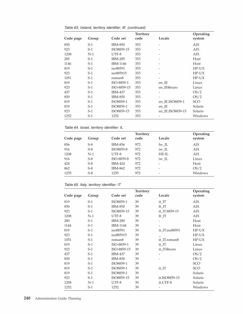
Table
63.
Ireland,
territory
identifier:
IE
(continued)
Code
page
Group
Code
set
Territory
code
Locale
Operating
system
850
S-1
IBM-850
353
-
AIX
923
S-1
ISO8859-15
353
-
AIX
1208
N-1
UTF-8
353
-
AIX
285
S-1
IBM-285
353
-
Host
1146
S-1
IBM-1146
353
-
Host
819
S-1
iso88591
353
-
HP-UX
923
S-1
iso885915
353
-
HP-UX
1051
S-1
roman8
353
-
HP-UX
819
S-1
ISO-8859-1
353
en_IE
Linux
923
S-1
ISO-8859-15
353
en_IE@euro
Linux
437
S-1
IBM-437
353
-
OS/2
850
S-1
IBM-850
353
-
OS/2
819
S-1
ISO8859-1
353
en_IE.ISO8859-1
SCO
819
S-1
ISO8859-1
353
en_IE
Solaris
923
S-1
ISO8859-15
353
en_IE.ISO8859-15
Solaris
1252
S-1
1252
353
-
Windows
Table
64.
Israel,
territory
identifier:
IL
Code
page
Group
Code
set
Territory
code
Locale
Operating
system
856
S-8
IBM-856
972
Iw_IL
AIX
916
S-8
ISO8859-8
972
iw_IL
AIX
1208
N-1
UTF-8
972
HE-IL
AIX
916
S-8
ISO-8859-8
972
iw_IL
Linux
424
S-8
IBM-424
972
-
Host
862
S-8
IBM-862
972
-
OS/2
1255
S-8
1255
972
-
Windows
Table
65.
Italy,
territory
identifier:
IT
Code
page
Group
Code
set
Territory
code
Locale
Operating
system
819
S-1
ISO8859-1
39
it_IT
AIX
850
S-1
IBM-850
39
It_IT
AIX
923
S-1
ISO8859-15
39
it_IT.8859-15
AIX
1208
N-1
UTF-8
39
It_IT
AIX
280
S-1
IBM-280
39
-
Host
1144
S-1
IBM-1144
39
-
Host
819
S-1
iso88591
39
it_IT.iso88591
HP-UX
923
S-1
iso885915
39
_
HP-UX
1051
S-1
roman8
39
it_IT.roman8
HP-UX
819
S-1
ISO-8859-1
39
it_IT
Linux
923
S-1
ISO-8859-15
39
it_IT@euro
Linux
437
S-1
IBM-437
39
-
OS/2
850
S-1
IBM-850
39
-
OS/2
819
S-1
ISO8859-1
39
SCO
819
S-1
ISO8859-1
39
it_IT
SCO
819
S-1
ISO8859-1
39
Solaris
923
S-1
ISO8859-15
39
it.ISO8859-15
Solaris
1208
N-1
UTF-8
39
it.UTF-8
Solaris
1252
S-1
1252
39
-
Windows
240
Administration
Guide:
Planning

Table
66.
Japan,
territory
identifier:
JP
Code
page
Group
Code
set
Territory
code
Locale
Operating
system
932
D-1
IBM-932
81
Ja_JP
AIX
943
D-1
IBM-943
81
Ja_JP
AIX
See
note
2
on
page
250.
954
D-1
IBM-eucJP
81
ja_JP
AIX
1208
N-1
UTF-8
81
JA_JP
AIX
930
D-1
IBM-930
81
-
Host
939
D-1
IBM-939
81
-
Host
5026
D-1
IBM-5026
81
-
Host
5035
D-1
IBM-5035
81
-
Host
1390
D-1
81
-
Host
1399
D-1
81
-
Host
954
D-1
eucJP
81
ja_JP.eucJP
HP-UX
5039
D-1
SJIS
81
ja_JP.SJIS
HP-UX
954
D-1
EUC-JP
81
ja_JP
Linux
932
D-1
IBM-932
81
-
OS/2
942
D-1
IBM-942
81
-
OS/2
943
D-1
IBM-943
81
-
OS/2
954
D-1
eucJP
81
ja
SCO
954
D-1
eucJP
81
ja_JP
SCO
954
D-1
eucJP
81
ja_JP.EUC
SCO
954
D-1
eucJP
81
ja_JP.eucJP
SCO
943
D-1
IBM-943
81
ja_JP.PCK
Solaris
954
D-1
eucJP
81
ja
Solaris
954
D-1
eucJP
81
japanese
Solaris
1208
N-1
UTF-8
81
ja_JP.UTF-8
Solaris
943
D-1
IBM-943
81
-
Windows
1394
D-1
81
-
See
note
3
on
page
250.
Table
67.
Kazakhstan,
territory
identifier:
KZ
Code
page
Group
Code
set
Territory
code
Locale
Operating
system
1251
S-5
1251
7
-
Windows
Table
68.
Korea,
South,
territory
identifier:
KR
Code
page
Group
Code
set
Territory
code
Locale
Operating
system
970
D-3
IBM-eucKR
82
ko_KR
AIX
1208
N-1
UTF-8
82
KO_KR
AIX
933
D-3
IBM-933
82
-
Host
1364
D-3
IBM-1364
82
-
Host
970
D-3
eucKR
82
ko_KR.eucKR
HP-UX
970
D-3
EUC-KR
82
ko_KR
Linux
949
D-3
IBM-949
82
-
OS/2
970
D-3
eucKR
82
ko_KR.eucKR
SGI
970
D-3
5601
82
ko
Solaris
1208
N-1
UTF-8
82
ko.UTF-8
Solaris
1363
D-3
1363
82
-
Windows
Appendix
B.
National
language
support
(NLS)
241

Table
69.
Latin
America,
territory
identifier:
Lat
Code
page
Group
Code
set
Territory
code
Locale
Operating
system
819
S-1
ISO8859-1
3
-
AIX
850
S-1
IBM-850
3
-
AIX
923
S-1
ISO8859-15
3
-
AIX
1208
N-1
UTF-8
3
-
AIX
284
S-1
IBM-284
3
-
Host
1145
S-1
IBM-1145
3
-
Host
819
S-1
iso88591
3
-
HP-UX
923
S-1
iso885915
3
-
HP-UX
1051
S-1
roman8
3
-
HP-UX
819
S-1
ISO-8859-1
3
-
Linux
923
S-1
ISO-8859-15
3
-
Linux
437
S-1
IBM-437
3
-
OS/2
850
S-1
IBM-850
3
-
OS/2
819
S-1
ISO8859-1
3
-
Solaris
923
S-1
ISO8859-15
3
-
Solaris
1252
S-1
1252
3
-
Windows
Table
70.
Latvia,
territory
identifier:
LV
Code
page
Group
Code
set
Territory
code
Locale
Operating
system
921
S-10
IBM-921
371
Lv_LV
AIX
1208
N-1
UTF-8
371
LV_LV
AIX
1112
S-10
IBM-1112
371
-
Host
1156
S-10
IBM-1156
371
-
Host
921
S-10
IBM-921
371
-
OS/2
1257
S-10
1257
371
-
Windows
Table
71.
Lithunia,
territory
identifier:
LT
Code
page
Group
Code
set
Territory
code
Locale
Operating
system
921
S-10
IBM-921
370
Lt_LT
AIX
1208
N-1
UTF-8
370
LT_LT
AIX
1112
S-10
IBM-1112
370
-
Host
1156
S-10
IBM-1156
370
-
Host
921
S-10
IBM-921
370
-
OS/2
1257
S-10
1257
370
-
Windows
Table
72.
Malaysia,
territory
identifier:
ID
Code
page
Group
Code
set
Territory
code
Locale
Operating
system
1252
S-1
1252
60
-
Windows
Table
73.
Netherlands,
territory
identifier:
NL
Code
page
Group
Code
set
Territory
code
Locale
Operating
system
819
S-1
ISO8859-1
31
nl_NL
AIX
850
S-1
IBM-850
31
Nl_NL
AIX
923
S-1
ISO8859-15
31
nl_NL.8859-15
AIX
242
Administration
Guide:
Planning

Table
73.
Netherlands,
territory
identifier:
NL
(continued)
Code
page
Group
Code
set
Territory
code
Locale
Operating
system
1208
N-1
UTF-8
31
NL_NL
AIX
37
S-1
IBM-37
31
-
Host
1140
S-1
IBM-1140
31
-
Host
819
S-1
iso88591
31
nl_NL.iso88591
HP-UX
923
S-1
iso885915
31
_
HP-UX
1051
S-1
roman8
31
nl_NL.roman8
HP-UX
819
S-1
ISO-8859-1
31
nl_NL
Linux
923
S-1
ISO-8859-15
31
nl_NL@euro
Linux
437
S-1
IBM-437
31
-
OS/2
850
S-1
IBM-850
31
-
OS/2
819
S-1
ISO8859-1
31
nl
SCO
819
S-1
ISO8859-1
31
nl_NL
SCO
819
S-1
ISO8859-1
31
nl
Solaris
923
S-1
ISO8859-15
31
nl.ISO8859-15
Solaris
1252
S-1
1252
31
-
Windows
Table
74.
New
Zealand,
territory
identifier:
NZ
Code
page
Group
Code
set
Territory
code
Locale
Operating
system
819
S-1
ISO8859-1
64
-
AIX
850
S-1
IBM-850
64
-
AIX
923
S-1
ISO8859-15
64
-
AIX
1208
N-1
UTF-8
64
-
AIX
37
S-1
IBM-37
64
-
Host
1140
S-1
IBM-1140
64
-
Host
819
S-1
ISO8859-1
64
-
HP-UX
923
S-1
ISO8859-15
64
-
HP-UX
850
S-1
IBM-850
64
-
OS/2
819
S-1
ISO8859-1
64
en_NZ
SCO
819
S-1
ISO8859-1
64
en_NZ
Solaris
923
S-1
ISO8859-15
64
-
Solaris
1252
S-1
1252
64
-
Windows
Table
75.
Norway,
territory
identifier:
NO
Code
page
Group
Code
set
Territory
code
Locale
Operating
system
819
S-1
ISO8859-1
47
no_NO
AIX
850
S-1
IBM-850
47
No_NO
AIX
923
S-1
ISO8859-15
47
no_NO.8859-15
AIX
1208
N-1
UTF-8
47
NO_NO
AIX
277
S-1
IBM-277
47
-
Host
1142
S-1
IBM-1142
47
-
Host
819
S-1
iso88591
47
no_NO.iso88591
HP-UX
923
S-1
iso885915
47
-
HP-UX
1051
S-1
roman8
47
no_NO.roman8
HP-UX
819
S-1
ISO-8859-1
47
no_NO
Linux
923
S-1
ISO-8859-15
47
-
Linux
850
S-1
IBM-850
47
-
OS/2
819
S-1
ISO8859-1
47
no
SCO
819
S-1
ISO8859-1
47
no_NO
SCO
Appendix
B.
National
language
support
(NLS)
243

Table
75.
Norway,
territory
identifier:
NO
(continued)
Code
page
Group
Code
set
Territory
code
Locale
Operating
system
819
S-1
ISO8859-1
47
no
Solaris
923
S-1
ISO8859-15
47
-
Solaris
1252
S-1
1252
47
-
Windows
Table
76.
Poland,
territory
identifier:
PL
Code
page
Group
Code
set
Territory
code
Locale
Operating
system
912
S-2
ISO8859-2
48
pl_PL
AIX
1208
N-1
UTF-8
48
PL_PL
AIX
870
S-2
IBM-870
48
-
Host
1153
S-2
IBM-1153
48
-
Host
912
S-2
iso88592
48
pl_PL.iso88592
HP-UX
912
S-2
ISO-8859-2
48
pl_PL
Linux
852
S-2
IBM-852
48
-
OS/2
912
S-2
ISO8859-2
48
pl_PL.ISO8859-2
SCO
1250
S-2
1250
48
-
Windows
Table
77.
Portugal,
territory
identifier:
PT
Code
page
Group
Code
set
Territory
code
Locale
Operating
system
819
S-1
ISO8859-1
351
pt_PT
AIX
850
S-1
IBM-850
351
Pt_PT
AIX
923
S-1
ISO8859-15
351
pt_PT.8859-15
AIX
1208
N-1
UTF-8
351
PT_PT
AIX
37
S-1
IBM-37
351
-
Host
1140
S-1
IBM-1140
351
-
Host
819
S-1
iso88591
351
pt_PT.iso88591
HP-UX
923
S-1
iso885915
351
-
HP-UX
1051
S-1
roman8
351
pt_PT.roman8
HP-UX
819
S-1
ISO-8859-1
351
pt_PT
Linux
923
S-1
ISO-8859-15
351
pt_PT@euro
Linux
850
S-1
IBM-850
351
-
OS/2
860
S-1
IBM-860
351
-
OS/2
819
S-1
ISO8859-1
351
pt
SCO
819
S-1
ISO8859-1
351
pt_PT
SCO
819
S-1
ISO8859-1
351
pt
Solaris
923
S-1
ISO8859-15
351
pt.ISO8859-15
Solaris
1252
S-1
1252
351
-
Windows
Table
78.
Romania,
territory
identifier:
RO
Code
page
Group
Code
set
Territory
code
Locale
Operating
system
912
S-2
ISO8859-2
40
ro_RO
AIX
1208
N-1
UTF-8
40
RO_RO
AIX
870
S-2
IBM-870
40
-
Host
1153
S-2
IBM-1153
40
-
Host
912
S-2
iso88592
40
ro_RO.iso88592
HP-UX
912
S-2
ISO-8859-2
40
ro_RO
Linux
852
S-2
IBM-852
40
-
OS/2
244
Administration
Guide:
Planning

Table
78.
Romania,
territory
identifier:
RO
(continued)
Code
page
Group
Code
set
Territory
code
Locale
Operating
system
912
S-2
ISO8859-2
40
ro_RO.ISO8859-2
SCO
1250
S-2
1250
40
-
Windows
Table
79.
Russia,
territory
identifier:
RU
Code
page
Group
Code
set
Territory
code
Locale
Operating
system
915
S-5
ISO8859-5
7
ru_RU
AIX
1208
N-1
UTF-8
7
RU_RU
AIX
1025
S-5
IBM-1025
7
-
Host
1154
S-5
IBM-1154
7
-
Host
915
S-5
iso88595
7
ru_RU.iso88595
HP-UX
878
S-5
KOI8-R
7
ru_RU.koi8-r
Linux,
Solaris
915
S-5
ISO-8859-5
7
ru_RU
Linux
866
S-5
IBM-866
7
-
OS/2
915
S-5
ISO8859-5
7
-
OS/2
915
S-5
ISO8859-5
7
ru_RU.ISO8859-5
SCO
1251
S-5
1251
7
-
Windows
Table
80.
Serbia/Montenegro,
territory
identifier:
SP
Code
page
Group
Code
set
Territory
code
Locale
Operating
system
915
S-5
ISO8859-5
381
sr_SP
AIX
1208
N-1
UTF-8
381
SR_SP
AIX
1025
S-5
IBM-1025
381
-
Host
1154
S-5
IBM-1154
381
-
Host
915
S-5
iso88595
381
-
HP-UX
855
S-5
IBM-855
381
-
OS/2
915
S-5
ISO8859-5
381
-
OS/2
1251
S-5
1251
381
-
Windows
Table
81.
Slovakia,
territory
identifier:
SK
Code
page
Group
Code
set
Territory
code
Locale
Operating
system
912
S-2
ISO8859-2
422
sk_SK
AIX
1208
N-1
UTF-8
422
SK_SK
AIX
870
S-2
IBM-870
422
-
Host
1153
S-2
IBM-1153
422
-
Host
912
S-2
iso88592
422
sk_SK.iso88592
HP-UX
852
S-2
IBM-852
422
-
OS/2
912
S-2
ISO8859-2
422
sk_SK.ISO8859-2
SCO
1250
S-2
1250
422
-
Windows
Table
82.
Slovenia,
territory
identifier:
SI
Code
page
Group
Code
set
Territory
code
Locale
Operating
system
912
S-2
ISO8859-2
386
sl_SI
AIX
1208
N-1
UTF-8
386
SL_SI
AIX
Appendix
B.
National
language
support
(NLS)
245
|||||||

Table
82.
Slovenia,
territory
identifier:
SI
(continued)
Code
page
Group
Code
set
Territory
code
Locale
Operating
system
870
S-2
IBM-870
386
-
Host
1153
S-2
IBM-1153
386
-
Host
912
S-2
iso88592
386
sl_SI.iso88592
HP-UX
912
S-2
ISO-8859-2
386
sl_SI
Linux
852
S-2
IBM-852
386
-
OS/2
912
S-2
ISO8859-2
386
sl_SI.ISO8859-2
SCO
1250
S-2
1250
386
-
Windows
Table
83.
South
Africa,
territory
identifier:
ZA
Code
page
Group
Code
set
Territory
code
Locale
Operating
system
819
S-1
ISO8859-1
27
en_ZA
AIX
850
S-1
IBM-850
27
En_ZA
AIX
923
S-1
ISO8859-15
27
en_ZA.8859-15
AIX
1208
N-1
UTF-8
27
EN_ZA
AIX
285
S-1
IBM-285
27
-
Host
1146
S-1
IBM-1146
27
-
Host
819
S-1
iso88591
27
-
HP-UX
923
S-1
iso885915
27
-
HP-UX
1051
S-1
roman8
27
-
HP-UX
437
S-1
IBM-437
27
-
OS/2
850
S-1
IBM-850
27
-
OS/2
819
S-1
ISO8859-1
27
en_ZA.ISO8859-1
SCO
819
S-1
ISO8859-1
27
-
Solaris
923
S-1
ISO8859-15
27
-
Solaris
1252
S-1
1252
27
-
Windows
Table
84.
Spain,
territory
identifier:
ES
Code
page
Group
Code
set
Territory
code
Locale
Operating
system
819
S-1
ISO8859-1
34
es_ES
AIX
850
S-1
IBM-850
34
Es_ES
AIX
923
S-1
ISO8859-15
34
es_ES.8859-15
AIX
1208
N-1
UTF-8
34
ES_ES
AIX
284
S-1
IBM-284
34
-
Host
1145
S-1
IBM-1145
34
-
Host
819
S-1
iso88591
34
es_ES.iso88591
HP-UX
923
S-1
iso885915
34
-
HP-UX
1051
S-1
roman8
34
es_ES.roman8
HP-UX
819
S-1
ISO-8859-1
34
es_ES
Linux
923
S-1
ISO-8859-15
34
es_ES@euro
Linux
437
S-1
IBM-437
34
-
OS/2
850
S-1
IBM-850
34
-
OS/2
819
S-1
ISO8859-1
34
es
SCO
819
S-1
ISO8859-1
34
es_ES
SCO
819
S-1
ISO8859-1
34
es
Solaris
923
S-1
ISO8859-15
34
es.ISO8859-15
Solaris
1208
N-1
UTF-8
34
es.UTF-8
Solaris
1252
S-1
1252
34
-
Windows
246
Administration
Guide:
Planning

Table
85.
Spain
(Catalan),
territory
identifier:
ES
Code
page
Group
Code
set
Territory
code
Locale
Operating
system
819
S-1
ISO8859-1
34
ca_ES
AIX
850
S-1
IBM-850
34
Ca_ES
AIX
923
S-1
ISO8859-15
34
ca_ES.8859-15
AIX
1208
N-1
UTF-8
34
CA_ES
AIX
Table
86.
Sweden,
territory
identifier:
SE
Code
page
Group
Code
set
Territory
code
Locale
Operating
system
819
S-1
ISO8859-1
46
sv_SE
AIX
850
S-1
IBM-850
46
Sv_SE
AIX
923
S-1
ISO8859-15
46
sv_SE.8859-15
AIX
1208
N-1
UTF-8
46
SV_SE
AIX
278
S-1
IBM-278
46
-
Host
1143
S-1
IBM-1143
46
-
Host
819
S-1
iso88591
46
sv_SE.iso88591
HP-UX
923
S-1
iso885915
46
-
HP-UX
1051
S-1
roman8
46
sv_SE.roman8
HP-UX
819
S-1
ISO-8859-1
46
sv_SE
Linux
923
S-1
ISO-8859-15
46
-
Linux
437
S-1
IBM-437
46
-
OS/2
850
S-1
IBM-850
46
-
OS/2
819
S-1
ISO8859-1
46
sv
SCO
819
S-1
ISO8859-1
46
sv_SE
SCO
819
S-1
ISO8859-1
46
sv
Solaris
923
S-1
ISO8859-15
46
sv.ISO8859-15
Solaris
1208
N-1
UTF-8
46
sv.UTF-8
Solaris
1252
S-1
1252
46
-
Windows
Table
87.
Switzerland,
territory
identifier:
CH
Code
page
Group
Code
set
Territory
code
Locale
Operating
system
819
S-1
ISO8859-1
41
de_CH
AIX
850
S-1
IBM-850
41
De_CH
AIX
923
S-1
ISO8859-15
41
de_CH.8859-15
AIX
1208
N-1
UTF-8
41
DE_CH
AIX
500
S-1
IBM-500
41
-
Host
1148
S-1
IBM-1148
41
-
Host
819
S-1
iso88591
41
-
HP-UX
923
S-1
iso885915
41
-
HP-UX
1051
S-1
roman8
41
-
HP-UX
819
S-1
ISO-8859-1
41
de_CH
Linux
923
S-1
ISO-8859-15
41
-
Linux
437
S-1
IBM-437
41
-
OS/2
850
S-1
IBM-850
41
-
OS/2
819
S-1
ISO8859-1
41
de_CH
SCO
819
S-1
ISO8859-1
41
fr_CH
SCO
819
S-1
ISO8859-1
41
it_CH
SCO
819
S-1
ISO8859-1
41
de_CH
Solaris
923
S-1
ISO8859-15
41
-
Solaris
1252
S-1
1252
41
-
Windows
Appendix
B.
National
language
support
(NLS)
247

Table
88.
Taiwan,
territory
identifier:
TW
Code
page
Group
Code
set
Territory
code
Locale
Operating
system
950
D-2
big5
88
Zh_TW
AIX
See
note
8
on
page
251.
964
D-2
IBM-eucTW
88
zh_TW
AIX
1208
N-1
UTF-8
88
ZH_TW
AIX
937
D-2
IBM-937
88
-
Host
1371
D-2
IBM-1371
88
-
Host
950
D-2
big5
88
zh_TW.big5
HP-UX
964
D-2
eucTW
88
zh_TW.eucTW
HP-UX
950
D-2
BIG5
88
zh_TW
Linux
938
D-2
IBM-938
88
-
OS/2
948
D-2
IBM-948
88
-
OS/2
950
D-2
big5
88
-
OS/2
950
D-2
big5
88
zh_TW.BIG5
Solaris
964
D-2
cns11643
88
zh_TW
Solaris
1208
N-1
UTF-8
88
zh_TW.UTF-8
Solaris
950
D-2
big5
88
-
Windows
See
note
8
on
page
251.
Table
89.
Thailand,
territory
identifier:
TH
Code
page
Group
Code
set
Territory
code
Locale
Operating
system
874
S-20
TIS620-1
66
th_TH
AIX
1208
N-1
UTF-8
66
TH_TH
AIX
838
S-20
IBM-838
66
-
Host
1160
S-20
IBM-1160
66
-
Host
874
S-20
tis620
66
th_TH.tis620
HP-UX
874
S-20
TIS620-1
66
-
OS/2
874
S-20
TIS620-1
66
-
Windows
Table
90.
Turkey,
territory
identifier:
TR
Code
page
Group
Code
set
Territory
code
Locale
Operating
system
920
S-9
ISO8859-9
90
tr_TR
AIX
1208
N-1
UTF-8
90
TR_TR
AIX
1026
S-9
IBM-1026
90
-
Host
1155
S-9
IBM-1155
90
-
Host
920
S-9
iso88599
90
tr_TR.iso88599
HP-UX
920
S-9
ISO-8859-9
90
tr_TR
Linux
857
S-9
IBM-857
90
-
OS/2
920
S-9
ISO8859-9
90
tr_TR.ISO8859-9
SCO
1254
S-9
1254
90
-
Windows
Table
91.
United
Kingdom,
territory
identifier:
GB
Code
page
Group
Code
set
Territory
code
Locale
Operating
system
819
S-1
ISO8859-1
44
en_GB
AIX
850
S-1
IBM-850
44
En_GB
AIX
248
Administration
Guide:
Planning

Table
91.
United
Kingdom,
territory
identifier:
GB
(continued)
Code
page
Group
Code
set
Territory
code
Locale
Operating
system
923
S-1
ISO8859-15
44
en_GB.8859-15
AIX
1208
N-1
UTF-8
44
EN_GB
AIX
285
S-1
IBM-285
44
-
Host
1146
S-1
IBM-1146
44
-
Host
819
S-1
iso88591
44
en_GB.iso88591
HP-UX
923
S-1
iso885915
44
-
HP-UX
1051
S-1
roman8
44
en_GB.roman8
HP-UX
819
S-1
ISO-8859-1
44
en_GB
Linux
923
S-1
ISO-8859-15
44
-
Linux
437
S-1
IBM-437
44
-
OS/2
850
S-1
IBM-850
44
-
OS/2
819
S-1
ISO8859-1
44
en_GB
SCO
819
S-1
ISO8859-1
44
en
SCO
819
S-1
ISO8859-1
44
en_GB
Solaris
923
S-1
ISO8859-15
44
en_GB.ISO8859-15
Solaris
1252
S-1
1252
44
-
Windows
Table
92.
Ukraine,
territory
identifier:
UA
Code
page
Group
Code
set
Territory
code
Locale
Operating
system
1124
S-12
IBM-1124
380
Uk_UA
AIX
1208
N-1
UTF-8
380
UK_UA
AIX
1123
S-12
IBM-1123
380
-
Host
1158
S-12
IBM-1158
380
-
Host
1168
S-12
KOI8-U
380
uk_UA.koi8u
Linux
1125
S-12
IBM-1125
380
-
OS/2
1251
S-12
1251
380
-
Windows
Table
93.
United
States
of
America,
territory
identifier:
US
Code
page
Group
Code
set
Territory
code
Locale
Operating
system
819
S-1
ISO8859-1
1
en_US
AIX
850
S-1
IBM-850
1
En_US
AIX
923
S-1
ISO8859-15
1
en_US.8859-15
AIX
1208
N-1
UTF-8
1
EN_US
AIX
37
S-1
IBM-37
1
-
Host
1140
S-1
IBM-1140
1
-
Host
819
S-1
iso88591
1
en_US.iso88591
HP-UX
923
S-1
iso885915
1
-
HP-UX
1051
S-1
roman8
1
en_US.roman8
HP-UX
819
S-1
ISO-8859-1
1
en_US
Linux
923
S-1
ISO-8859-15
1
-
Linux
437
S-1
IBM-437
1
-
OS/2
850
S-1
IBM-850
1
-
OS/2
819
S-1
ISO8859-1
1
en_US
SCO
819
S-1
ISO8859-1
1
en_US
SGI
819
S-1
ISO8859-1
1
en_US
Solaris
923
S-1
ISO8859-15
1
en_US.ISO8859-15
Solaris
1208
N-1
UTF-8
1
en_US.UTF-8
Solaris
1252
S-1
1252
1
-
Windows
Appendix
B.
National
language
support
(NLS)
249
||||||

Table
94.
Vietnam,
territory
identifier:
VN
Code
page
Group
Code
set
Territory
code
Locale
Operating
system
1129
S-11
IBM-1129
84
Vi_VN
AIX
1208
N-1
UTF-8
84
VI_VN
AIX
1130
S-11
IBM-1130
84
-
Host
1164
S-11
IBM-1164
84
-
Host
1129
S-11
IBM-1129
84
-
OS/2
1258
S-11
1258
84
-
Windows
Notes:
1.
CCSIDs
1392
and
5488
(GB
18030)
can
only
be
used
with
the
load
or
import
utilities
to
move
data
from
CCSIDs
1392
and
5488
to
a
DB2
UDB
Unicode
database,
or
to
export
from
a
DB2
UDB
Unicode
database
to
CCSIDs
1392
or
5488.
2.
On
AIX
4.3
or
later
the
code
page
is
943.
If
you
are
using
AIX
4.2
or
earlier,
the
code
page
is
932.
3.
Code
page
1394
(Shift
JIS
X0213)
can
only
be
used
with
the
load
or
import
utilities
to
move
data
from
code
page
1394
to
a
DB2
UDB
Unicode
database,
or
to
export
from
a
DB2
UDB
Unicode
database
to
code
page
1394.
4.
The
following
map
to
Arabic
Countries/Regions
(AA):
v
Arabic
(Saudi
Arabia)
v
Arabic
(Iraq)
v
Arabic
(Egypt)
v
Arabic
(Libya)
v
Arabic
(Algeria)
v
Arabic
(Morocco)
v
Arabic
(Tunisia)
v
Arabic
(Oman)
v
Arabic
(Yemen)
v
Arabic
(Syria)
v
Arabic
(Jordan)
v
Arabic
(Lebanon)
v
Arabic
(Kuwait)
v
Arabic
(United
Arab
Emirates)
v
Arabic
(Bahrain)
v
Arabic
(Qatar)5.
The
following
map
to
English
(US):
v
English
(Jamaica)
v
English
(Caribbean)6.
The
following
map
to
Latin
America
(Lat):
v
Spanish
(Mexican)
v
Spanish
(Guatemala)
v
Spanish
(Costa
Rica)
v
Spanish
(Panama)
v
Spanish
(Dominican
Republic)
250
Administration
Guide:
Planning

v
Spanish
(Venezuela)
v
Spanish
(Colombia)
v
Spanish
(Peru)
v
Spanish
(Argentina)
v
Spanish
(Ecuador)
v
Spanish
(Chile)
v
Spanish
(Uruguay)
v
Spanish
(Paraguay)
v
Spanish
(Bolivia)7.
The
following
Indic
scripts
are
supported
through
Unicode:
Hindi,
Gujarati,
Kannada,
Konkani,
Marathi,
Punjabi,
Sanskrit,
Tamil
and
Telugu.
8.
Code
page
950
is
also
known
as
Big5.
Microsoft
code
page
950
differs
from
IBM
code
page
950
in
the
following
ways:
Range
Description
IBM
Microsoft
Difference
X’8140’
to
X’8DFE’
User
defined
characters
User
defined
area
User
defined
area
Same
X’8E40’
to
X’A0FE’
User
defined
characters
User
defined
area
User
defined
area
Same
X’A140’
to
X’A3BF’
Special
symbols
System
characters
System
characters
Same
X’A3C0’
to
X’A3E0’
Control
symbols
System
characters
Empty
Different
X’A3E1’
to
X’A3FE’
Reserved
Empty
Empty
Same
X’A440’
to
X’C67E’
Primary
use
characters
System
characters
System
characters
Same
X’C6A1’
to
X’C878’
Eten
added
symbols
System
characters
User
defined
area
Different
X’C879’
to
X’C8CC’
Eten
added
symbols
Empty
User
defined
area
Different
X’C8CD’
to
X’C8D3’
Eten
added
symbols
System
characters
User
defined
area
Different
X’C8D4’
to
X’C8FD’
Reserved
System
characters
User
defined
area
Different
X’C8FE’
Invalid/
undefined
character
System
characters
User
defined
area
Different
X’C940’
to
X’F9D5’
Secondary
use
characters
System
characters
System
characters
Same
X’F9D6’
to
X’F9FE’
Eten
extension
for
Big-5
User
defined
area
System
characters
Different
X’FA40’
to
X’FEFE’
User
defined
characters
User
defined
area
User
defined
area
Same
X’8181’
to
X’8C82’
User
defined
characters
User
defined
area
Empty
Different
X’F286’
to
X’F9A0’
IBM
select
characters
System
characters
Empty
Different
Total
characters
14
060
13
502
Total
user
defined
characters
6
204
6
217
Total
defined
code
points
20
264
19
719
Appendix
B.
National
language
support
(NLS)
251

Related
tasks:
v
“Installing
the
previous
tables
for
converting
between
code
page
1394
and
Unicode”
on
page
280
Enabling
and
disabling
euro
symbol
support
DB2
Universal
Database™
(DB2
UDB)
provides
support
for
the
euro
currency
symbol.
The
euro
symbol
has
been
added
to
numerous
code
pages.
Many
DB2
UDB
internal
code
page
conversion
tables,
and
many
external
code
page
conversion
table
files
located
in
the
sqllib/conv/
directory
have
been
enhanced
to
support
the
euro
symbol.
Microsoft
ANSI
code
pages
have
been
modified
to
include
the
euro
currency
symbol
in
position
X’80’.
Code
page
850
has
been
modified
to
replace
the
character
DOTLESS
I
(found
at
position
X’D5’)
with
the
euro
currency
symbol.
DB2
UDB
internal
code
page
conversion
routines
use
these
revised
code
page
definitions
as
the
default
to
provide
euro
symbol
support.
However,
if
you
want
to
use
the
non-euro
definitions
of
the
code
page
conversion
tables,
follow
the
procedure
below
after
installation
is
complete.
Prerequisites:
For
replacing
existing
external
code
page
conversion
table
files,
you
may
want
to
back
up
the
current
files
before
copying
the
non-euro
versions
over
them.
The
files
are
located
in
the
directory
sqllib/conv/.
On
UNIX,
sqllib/conv/
is
linked
to
the
install
path
of
DB2
UDB.
Procedure:
To
disable
euro-symbol
support:
1.
Stop
the
DB2
UDB
instance.
2.
Download
the
appropriate
conversion
table
files,
in
binary:
v
For
big-endian
platforms
from
ftp://ftp.software.ibm.com/ps/products/db2/info/vr8/conv/BigEndian/.
This
ftp
server
is
anonymous,
so
if
you
are
connecting
via
the
command
line,
log
in
as
user
″anonymous″
and
use
your
address
as
your
password.
After
logging
in,
change
to
the
conversion
tables
directory:
cd
ps/products/db2/info/vr8/conv/BigEndian/
v
For
little-endian
platforms
from
ftp://ftp.software.ibm.com/ps/products/db2/info/vr8/conv/LittleEndian/.
This
ftp
server
is
anonymous,
so
if
you
are
connecting
via
the
command
line,
log
in
as
user
″anonymous″
and
use
your
address
as
your
password.
After
logging
in,
change
to
the
conversion
tables
directory:
cd
ps/products/db2/info/vr8/conv/LittleEndian3.
Copy
the
files
to
your
sqllib/conv/
directory.
4.
Restart
the
DB2
UDB
instance.
Code
pages
819
and
1047:
For
code
pages
819
(ISO
8859-1
Latin
1
ASCII)
and
1047
(Latin
1
Open
System
EBCDIC),
the
euro
replacement
code
pages,
923
(ISO
8859-15
Latin
9
ASCII)
and
924
(Latin
9
Open
System
EBCDIC)
respectively,
contain
not
just
the
euro
symbol
252
Administration
Guide:
Planning
|||||
|
||||||
||||||

but
also
several
new
characters.
DB2
UDB
continues
to
use
the
old
(non-euro)
definitions
of
these
two
code
pages
and
conversion
tables,
namely
819
and
1047,
by
default.
There
are
two
ways
to
activate
the
new
923/924
code
page
and
the
associated
conversion
tables:
v
Create
a
new
database
that
uses
the
new
code
page.
For
example,
DB2
CREATE
DATABASE
dbname
USING
CODESET
ISO8859-15
TERRITORY
US
v
Rename
or
copy
the
923
or
924
conversion
table
file
in
the
sqllib/conv/
directory
to
819
or
1047,
respectively.
Related
concepts:
v
“Character
conversion”
in
the
SQL
Reference,
Volume
1
Related
reference:
v
“Conversion
tables
for
code
pages
923
and
924”
on
page
260
v
“Conversion
table
files
for
euro-enabled
code
pages”
on
page
253
Conversion
table
files
for
euro-enabled
code
pages
The
following
tables
list
the
conversion
tables
that
have
been
enhanced
to
support
the
euro
currency
symbol.
If
you
want
to
disable
euro
symbol
support,
download
the
conversion
table
file
indicated
in
the
column
titled
″Conversion
table
file″.
Arabic:
Database
server
CCSIDs/CPGIDs
Database
client
CCSIDs/CPGIDs
Conversion
table
files
420,
16804
1046,
9238
04201046.cnv,
IBM00420.ucs
420,
16804
1256,
5352
04201256.cnv,
IBM00420.ucs
420,
16804
1200,
1208,
13488,
17584
IBM00420.ucs
864,
17248
1046,
9238
08641046.cnv,
10460864.cnv,
IBM00864.ucs
864,
17248
1256,
5352
08641256.cnv,
12560864.cnv,
IBM00864.ucs
864,
17248
1200,
1208,
13488,
17584
IBM00864.ucs
1046,
9238
864,
17248
10460864.cnv,
08641046.cnv,
IBM01046.ucs
1046,
9238
1089
10461089.cnv,
10891046.cnv,
IBM01046.ucs
1046,
9238
1256,
5352
10461256.cnv,
12561046.cnv,
IBM01046.ucs
1046,
9238
1200,
1208,
13488,
17584
IBM01046.ucs
1089
1046,
9238
10891046.cnv,
10461089.cnv
1256,
5352
864,
17248
12560864.cnv,
08641256.cnv,
IBM01256.ucs
1256,
5352
1046,
9238
12561046.cnv,
10461256.cnv,
IBM01256.ucs
1256,
5352
1200,
1208,
13488,
17584
IBM01256.ucs
Appendix
B.
National
language
support
(NLS)
253
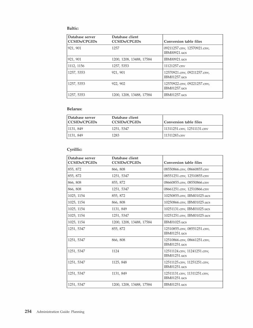
Baltic:
Database
server
CCSIDs/CPGIDs
Database
client
CCSIDs/CPGIDs
Conversion
table
files
921,
901
1257
09211257.cnv,
12570921.cnv,
IBM00921.ucs
921,
901
1200,
1208,
13488,
17584
IBM00921.ucs
1112,
1156
1257,
5353
11121257.cnv
1257,
5353
921,
901
12570921.cnv,
09211257.cnv,
IBM01257.ucs
1257,
5353
922,
902
12570922.cnv,
09221257.cnv,
IBM01257.ucs
1257,
5353
1200,
1208,
13488,
17584
IBM01257.ucs
Belarus:
Database
server
CCSIDs/CPGIDs
Database
client
CCSIDs/CPGIDs
Conversion
table
files
1131,
849
1251,
5347
11311251.cnv,
12511131.cnv
1131,
849
1283
11311283.cnv
Cyrillic:
Database
server
CCSIDs/CPGIDs
Database
client
CCSIDs/CPGIDs
Conversion
table
files
855,
872
866,
808
08550866.cnv,
08660855.cnv
855,
872
1251,
5347
08551251.cnv,
12510855.cnv
866,
808
855,
872
08660855.cnv,
08550866.cnv
866,
808
1251,
5347
08661251.cnv,
12510866.cnv
1025,
1154
855,
872
10250855.cnv,
IBM01025.ucs
1025,
1154
866,
808
10250866.cnv,
IBM01025.ucs
1025,
1154
1131,
849
10251131.cnv,
IBM01025.ucs
1025,
1154
1251,
5347
10251251.cnv,
IBM01025.ucs
1025,
1154
1200,
1208,
13488,
17584
IBM01025.ucs
1251,
5347
855,
872
12510855.cnv,
08551251.cnv,
IBM01251.ucs
1251,
5347
866,
808
12510866.cnv,
08661251.cnv,
IBM01251.ucs
1251,
5347
1124
12511124.cnv,
11241251.cnv,
IBM01251.ucs
1251,
5347
1125,
848
12511125.cnv,
11251251.cnv,
IBM01251.ucs
1251,
5347
1131,
849
12511131.cnv,
11311251.cnv,
IBM01251.ucs
1251,
5347
1200,
1208,
13488,
17584
IBM01251.ucs
254
Administration
Guide:
Planning
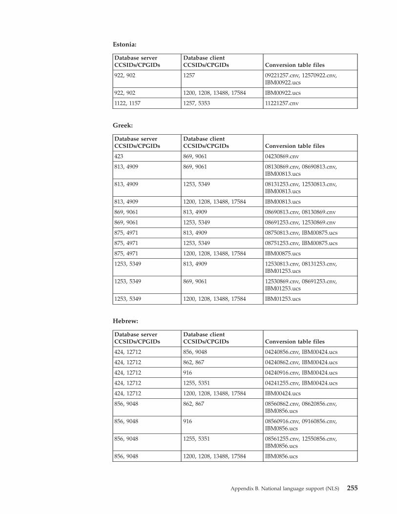
Estonia:
Database
server
CCSIDs/CPGIDs
Database
client
CCSIDs/CPGIDs
Conversion
table
files
922,
902
1257
09221257.cnv,
12570922.cnv,
IBM00922.ucs
922,
902
1200,
1208,
13488,
17584
IBM00922.ucs
1122,
1157
1257,
5353
11221257.cnv
Greek:
Database
server
CCSIDs/CPGIDs
Database
client
CCSIDs/CPGIDs
Conversion
table
files
423
869,
9061
04230869.cnv
813,
4909
869,
9061
08130869.cnv,
08690813.cnv,
IBM00813.ucs
813,
4909
1253,
5349
08131253.cnv,
12530813.cnv,
IBM00813.ucs
813,
4909
1200,
1208,
13488,
17584
IBM00813.ucs
869,
9061
813,
4909
08690813.cnv,
08130869.cnv
869,
9061
1253,
5349
08691253.cnv,
12530869.cnv
875,
4971
813,
4909
08750813.cnv,
IBM00875.ucs
875,
4971
1253,
5349
08751253.cnv,
IBM00875.ucs
875,
4971
1200,
1208,
13488,
17584
IBM00875.ucs
1253,
5349
813,
4909
12530813.cnv,
08131253.cnv,
IBM01253.ucs
1253,
5349
869,
9061
12530869.cnv,
08691253.cnv,
IBM01253.ucs
1253,
5349
1200,
1208,
13488,
17584
IBM01253.ucs
Hebrew:
Database
server
CCSIDs/CPGIDs
Database
client
CCSIDs/CPGIDs
Conversion
table
files
424,
12712
856,
9048
04240856.cnv,
IBM00424.ucs
424,
12712
862,
867
04240862.cnv,
IBM00424.ucs
424,
12712
916
04240916.cnv,
IBM00424.ucs
424,
12712
1255,
5351
04241255.cnv,
IBM00424.ucs
424,
12712
1200,
1208,
13488,
17584
IBM00424.ucs
856,
9048
862,
867
08560862.cnv,
08620856.cnv,
IBM0856.ucs
856,
9048
916
08560916.cnv,
09160856.cnv,
IBM0856.ucs
856,
9048
1255,
5351
08561255.cnv,
12550856.cnv,
IBM0856.ucs
856,
9048
1200,
1208,
13488,
17584
IBM0856.ucs
Appendix
B.
National
language
support
(NLS)
255

Database
server
CCSIDs/CPGIDs
Database
client
CCSIDs/CPGIDs
Conversion
table
files
862,
867
856,
9048
08620856.cnv,
08560862.cnv,
IBM00862.ucs
862,
867
916
08620916.cnv,
09160862.cnv,
IBM00862.ucs
862,
867
1255,
5351
08621255.cnv,
12550862.cnv,
IBM00862.ucs
862,
867
1200,
1208,
13488,
17584
IBM00862.ucs
916
856,
9048
09160856.cnv,
08560916.cnv
916
862,
867
09160862.cnv,
08620916.cnv
1255,
5351
856,
9048
12550856.cnv,
08561255.cnv,
IBM01255.ucs
1255,
5351
862,
867
12550862.cnv,
08621255.cnv,
IBM01255.ucs
1255,
5351
1200,
1208,
13488,
17584
IBM01255.ucs
Japanese:
Database
server
CCSIDs/CPGIDs
Database
client
CCSIDs/CPGIDs
Conversion
table
files
290,
8482
850,
858
02900850.cnv
1027,
5123
850,
858
10270850.cnv
Latin-1:
Database
server
CCSIDs/CPGIDs
Database
client
CCSIDs/CPGIDs
Conversion
table
files
37,
1140
437
00370437.cnv,
IBM00037.ucs
37,
1140
850,
858
00370850.cnv,
IBM00037.ucs
37,
1140
860
00370860.cnv,
IBM00037.ucs
37,
1140
1051
00371051.cnv,
IBM00037.ucs
37,
1140
1252,
5348
00371252.cnv,
IBM00037.ucs
37,
1140
1275
00371275.cnv,
IBM00037.ucs
37,
1140
1200,
1208,
13488,
17584
IBM00037.ucs
273,
1141
437
02730437.cnv,
IBM00273.ucs
273,
1141
850,
858
02730850.cnv,
IBM00273.ucs
273,
1141
1051
02731051.cnv,
IBM00273.ucs
273,
1141
1252,
5348
02731252.cnv,
IBM00273.ucs
273,
1141
1275
02731275.cnv,
IBM00273.ucs
273,
1141
1200,
1208,
13488,
17584
IBM00273.ucs
277,
1142
437
02770437.cnv,
IBM00277.ucs
277,
1142
850,
858
02770850.cnv,
IBM00277.ucs
277,
1142
1051
02771051.cnv,
IBM00277.ucs
277,
1142
1252,
5348
02771252.cnv,
IBM00277.ucs
256
Administration
Guide:
Planning

Database
server
CCSIDs/CPGIDs
Database
client
CCSIDs/CPGIDs
Conversion
table
files
277,
1142
1275
02771275.cnv,
IBM00277.ucs
277,
1142
1200,
1208,
13488,
17584
IBM00277.ucs
278,
1143
437
02780437.cnv,
IBM00278.ucs
278,
1143
850,
858
02780850.cnv,
IBM00278.ucs
278,
1143
1051
02781051.cnv,
IBM00278.ucs
278,
1143
1252,
5348
02781252.cnv,
IBM00278.ucs
278,
1143
1275
02781275.cnv,
IBM00278.ucs
278,
1143
1200,
1208,
13488,
17584
IBM00278.ucs
280,
1144
437
02800437.cnv,
IBM00280.ucs
280,
1144
850,
858
02800850.cnv,
IBM00280.ucs
280,
1144
1051
02801051.cnv,
IBM00280.ucs
280,
1144
1252,
5348
02801252.cnv,
IBM00280.ucs
280,
1144
1275
02801275.cnv,
IBM00280.ucs
280,
1144
1200,
1208,
13488,
17584
IBM00280.ucs
284,
1145
437
02840437.cnv,
IBM00284.ucs
284,
1145
850,
858
02840850.cnv,
IBM00284.ucs
284,
1145
1051
02841051.cnv,
IBM00284.ucs
284,
1145
1252,
5348
02841252.cnv,
IBM00284.ucs
284,
1145
1275
02841275.cnv,
IBM00284.ucs
284,
1145
1200,
1208,
13488,
17584
IBM00284.ucs
285,
1146
437
02850437.cnv,
IBM00285.ucs
285,
1146
850,
858
02850850.cnv,
IBM00285.ucs
285,
1146
1051
02851051.cnv,
IBM00285.ucs
285,
1146
1252,
5348
02851252.cnv,
IBM00285.ucs
285,
1146
1275
02851275.cnv,
IBM00285.ucs
285,
1146
1200,
1208,
13488,
17584
IBM00285.ucs
297,
1147
437
02970437.cnv,
IBM00297.ucs
297,
1147
850,
858
02970850.cnv,
IBM00297.ucs
297,
1147
1051
02971051.cnv,
IBM00297.ucs
297,
1147
1252,
5348
02971252.cnv,
IBM00297.ucs
297,
1147
1275
02971275.cnv,
IBM00297.ucs
297,
1147
1200,
1208,
13488,
17584
IBM00297.ucs
437
850,
858
04370850.cnv,
08500437.cnv
500,
1148
437
05000437.cnv,
IBM00500.ucs
500,
1148
850,
858
05000850.cnv,
IBM00500.ucs
500,
1148
857,
9049
05000857.cnv,
IBM00500.ucs
500,
1148
920
05000920.cnv,
IBM00500.ucs
500,
1148
1051
05001051.cnv,
IBM00500.ucs
500,
1148
1114,
5210
05001114.cnv,
IBM00500.ucs
500,
1148
1252,
5348
05001252.cnv,
IBM00500.ucs
Appendix
B.
National
language
support
(NLS)
257

Database
server
CCSIDs/CPGIDs
Database
client
CCSIDs/CPGIDs
Conversion
table
files
500,
1148
1254,
5350
05001254.cnv,
IBM00500.ucs
500,
1148
1275
05001275.cnv,
IBM00500.ucs
500,
1148
1200,
1208,
13488,
17584
IBM00500.ucs
850,
858
437
08500437.cnv,
04370850.cnv
850,
858
860
08500860.cnv,
08600850.cnv
850,
858
1114,
5210
08501114.cnv,
11140850.cnv
850,
858
1275
08501275.cnv,
12750850.cnv
860
850,
858
08600850.cnv,
08500860.cnv
871,
1149
437
08710437.cnv,
IBM00871.ucs
871,
1149
850,
858
08710850.cnv,
IBM00871.ucs
871,
1149
1051
08711051.cnv,
IBM00871.ucs
871,
1149
1252,
5348
08711252.cnv,
IBM00871.ucs
871,
1149
1275
08711275.cnv,
IBM00871.ucs
871,
1149
1200,
1208,
13488,
17584
IBM00871.ucs
1275
850,
858
12750850.cnv,
08501275.cnv
Latin-2:
Database
server
CCSIDs/CPGIDs
Database
client
CCSIDs/CPGIDs
Conversion
table
files
852,
9044
1250,
5346
08521250.cnv,
12500852.cnv
870,
1153
852,
9044
08700852.cnv,
IBM00870.ucs
870,
1153
1250,
5346
08701250.cnv,
IBM00870.ucs
870,
1153
1200,
1208,
13488,
17584
IBM00870.ucs
1250,
5346
852,
9044
12500852.cnv,
08521250.cnv,
IBM01250.ucs
1250,
5346
1200,
1208,
13488,
17584
IBM01250.ucs
Simplified
Chinese:
Database
server
CCSIDs/CPGIDs
Database
client
CCSIDs/CPGIDs
Conversion
table
files
837,
935,
1388
1200,
1208,
13488,
17584
1388ucs2.cnv
1386
1200,
1208,
13488,
17584
1386ucs2.cnv,
ucs21386.cnv
Traditional
Chinese:
Database
server
CCSIDs/CPGIDs
Database
client
CCSIDs/CPGIDs
Conversion
table
files
937,
835,
1371
950,
1370
09370950.cnv,
0937ucs2.cnv
937,
835,
1371
1200,
1208,
13488,
17584
0937ucs2.cnv
1114,
5210
850,
858
11140850.cnv,
08501114.cnv
258
Administration
Guide:
Planning

Thailand:
Database
server
CCSIDs/CPGIDs
Database
client
CCSIDs/CPGIDs
Conversion
table
files
838,
1160
874,
1161
08380874.cnv,
IBM00838.ucs
838,
1160
1200,
1208,
13488,
17584
IBM00838.ucs
874,
1161
1200,
1208,
13488,
17584
IBM00874.ucs
Turkish:
Database
server
CCSIDs/CPGIDs
Database
client
CCSIDs/CPGIDs
Conversion
table
files
857,
9049
1254,
5350
08571254.cnv,
12540857.cnv
1026,
1155
857,
9049
10260857.cnv,
IBM01026.ucs
1026,
1155
1254,
5350
10261254.cnv,
IBM01026.ucs
1026,
1155
1200,
1208,
13488,
17584
IBM01026.ucs
1254,
5350
857,
9049
12540857.cnv,
08571254.cnv,
IBM01254.ucs
1254,
5350
1200,
1208,
13488,
17584
IBM01254.ucs
Ukraine:
Database
server
CCSIDs/CPGIDs
Database
client
CCSIDs/CPGIDs
Conversion
table
files
1123,
1158
1124
11231124.cnv
1123,
1158
1125,
848
11231125.cnv
1123,
1158
1251,
5347
11231251.cnv
1124
1251,
5347
11241251.cnv,
12511124.cnv
1125,
848
1251,
5347
11251251.cnv,
12511125.cnv
Unicode:
Database
server
CCSIDs/CPGIDs
Database
client
CCSIDs/CPGIDs
Conversion
table
files
1200,
1208,
13488,
17584
813,
4909
IBM00813.ucs
1200,
1208,
13488,
17584
862,
867
IBM00862.ucs
1200,
1208,
13488,
17584
864,
17248
IBM00864.ucs
1200,
1208,
13488,
17584
874,
1161
IBM00874.ucs
1200,
1208,
13488,
17584
921,
901
IBM00921.ucs
1200,
1208,
13488,
17584
922,
902
IBM00922.ucs
1200,
1208,
13488,
17584
1046,
9238
IBM01046.ucs
1200,
1208,
13488,
17584
1250,
5346
IBM01250.ucs
1200,
1208,
13488,
17584
1251,
5347
IBM01251.ucs
1200,
1208,
13488,
17584
1253,
5349
IBM01253.ucs
1200,
1208,
13488,
17584
1254,
5350
IBM01254.ucs
1200,
1208,
13488,
17584
1255,
5351
IBM01255.ucs
Appendix
B.
National
language
support
(NLS)
259

Database
server
CCSIDs/CPGIDs
Database
client
CCSIDs/CPGIDs
Conversion
table
files
1200,
1208,
13488,
17584
1256,
5352
IBM01256.ucs
1200,
1208,
13488,
17584
1386
ucs21386.cnv,
1386ucs2.cnv
Vietnamese:
Database
server
CCSIDs/CPGIDs
Database
client
CCSIDs/CPGIDs
Conversion
table
files
1130,
1164
1258,
5354
11301258.cnv
1258,
5354
1129,
1163
12581129.cnv
Related
concepts:
v
“Character
conversion”
in
the
SQL
Reference,
Volume
1
Related
tasks:
v
“Enabling
and
disabling
euro
symbol
support”
on
page
252
Conversion
tables
for
code
pages
923
and
924
The
following
is
a
list
of
all
the
code
page
conversion
table
files
that
are
associated
with
code
pages
923
and
924.
Each
file
is
of
the
form
XXXXYYYY.cnv
or
ibmZZZZZ.ucs,
where
XXXXX
is
the
source
code
page
number
and
YYYY
is
the
target
code
page
number.
The
file
ibmZZZZZ.ucs
supports
conversion
between
code
page
ZZZZZ
and
Unicode.
To
activate
a
particular
code
page
conversion
table,
rename
or
copy
that
conversion
table
file
to
its
new
name
as
shown
in
the
second
column.
For
example,
to
support
the
euro
symbol
when
connecting
a
8859-1/15
(Latin
1/9)
client
to
a
Windows
1252
database,
you
need
to
rename
or
copy
the
following
code
page
conversion
table
files
in
the
sqllib/conv/
directory:
v
09231252.cnv
to
08191252.cnv
v
12520923.cnv
to
12520819.cnv
v
ibm00923.ucs
to
ibm00819.ucs
923
and
924
conversion
table
files
in
the
sqlllib/conv/
directory
New
name
00370923.cnv
00370819.cnv
02730923.cnv
02730819.cnv
02770923.cnv
02770819.cnv
02780923.cnv
02780819.cnv
02800923.cnv
02800819.cnv
02840923.cnv
02840819.cnv
02850923.cnv
02850819.cnv
02970923.cnv
02970819.cnv
04370923.cnv
04370819.cnv
05000923.cnv
05000819.cnv
260
Administration
Guide:
Planning

923
and
924
conversion
table
files
in
the
sqlllib/conv/
directory
New
name
08500923.cnv
08500819.cnv
08600923.cnv
08600819.cnv
08630923.cnv
08630819.cnv
08710923.cnv
08710819.cnv
09230437.cnv
08190437.cnv
09230500.cnv
08190500.cnv
09230850.cnv
08190850.cnv
09230860.cnv
08190860.cnv
09230863.cnv
08190863.cnv
09231043.cnv
08191043.cnv
09231051.cnv
08191051.cnv
09231114.cnv
08191114.cnv
09231252.cnv
08191252.cnv
09231275.cnv
08191275.cnv
09241252.cnv
10471252.cnv
10430923.cnv
10430819.cnv
10510923.cnv
10510819.cnv
11140923.cnv
11140819.cnv
12520923.cnv
12520819.cnv
12750923.cnv
12750819.cnv
ibm00923.ucs
ibm00819.ucs
Related
concepts:
v
“Character
conversion”
in
the
SQL
Reference,
Volume
1
Related
tasks:
v
“Enabling
and
disabling
euro
symbol
support”
on
page
252
Choosing
a
language
for
your
database
When
you
create
a
database,
you
have
to
decide
what
language
your
data
will
be
stored
in.
When
you
create
a
database,
you
can
specify
the
territory
and
code
set.
The
territory
and
code
set
may
be
different
from
the
current
operating
system
settings.
If
you
do
not
explicitly
choose
a
territory
and
code
set
at
database
creation
time,
the
database
will
be
created
using
the
current
locale.
When
you
are
choosing
a
code
set,
make
sure
it
can
encode
all
the
characters
in
the
language
you
will
be
using.
Another
option
is
to
store
data
in
a
Unicode
database,
which
means
that
you
do
not
have
to
choose
a
specific
language;
Unicode
encoding
includes
characters
from
almost
all
of
the
living
languages
in
the
world.
Appendix
B.
National
language
support
(NLS)
261

Locale
setting
for
the
DB2
Administration
Server
Ensure
that
the
locale
of
the
DB2
Administration
Server
instance
is
compatible
with
the
locale
of
the
DB2
Universal
Database™
(DB2
UDB)
instance.
Otherwise,
the
DB2
UDB
instance
cannot
communicate
with
the
DB2
Administration
Server.
If
the
LANG
environment
variable
is
not
set
in
the
user
profile
of
the
DB2
Administration
Server,
the
DB2
Administration
Server
will
be
started
with
the
default
system
locale.
If
the
default
system
locale
is
not
defined,
the
DB2
Administration
Server
will
be
started
with
code
page
819.
If
the
DB2
UDB
instance
uses
one
of
the
DBCS
locales,
and
the
DB2
Administration
Server
is
started
with
code
page
819,
the
instance
will
not
be
able
to
communicate
with
the
DB2
Administration
Server.
The
locale
of
the
DB2
Administration
Server
and
the
locale
of
the
DB2
UDB
instance
must
be
compatible.
For
example,
on
a
Simplified
Chinese
Linux
system,
LANG=zh_CN
should
be
set
in
the
DB2
Administration
Server’s
user
profile.
Enabling
bidirectional
support
Bidirectional
layout
transformations
are
implemented
in
DB2
Universal
Database
using
the
new
Coded
Character
Set
Identifier
(CCSID)
definitions.
For
the
new
bidirectional-specific
CCSIDs,
layout
transformations
are
performed
instead
of,
or
in
addition
to,
code
page
conversions.
To
use
this
support,
the
DB2BIDI
registry
variable
must
be
set
to
YES.
By
default,
this
variable
is
not
set.
It
is
used
by
the
server
for
all
conversions,
and
can
only
be
set
when
the
server
is
started.
Setting
DB2BIDI
to
YES
may
have
some
performance
impact
because
of
additional
checking
and
layout
transformations.
Restrictions:
The
following
restrictions
apply:
v
If
you
select
a
CCSID
that
is
not
appropriate
for
the
code
page
or
string
type
of
your
client
platform,
you
may
get
unexpected
results.
If
you
select
an
incompatible
CCSID
(for
example,
the
Hebrew
CCSID
for
connection
to
an
Arabic
database),
or
if
DB2BIDI
has
not
been
set
for
the
server,
you
will
receive
an
error
message
when
you
try
to
connect.
v
The
DB2
Universal
Database™
(DB2
UDB)
Command
Line
Processor
on
the
Windows
operating
system
does
not
have
bidirectional
support.
v
CCSID
override
is
not
supported
for
cases
where
the
HOST
EBCDIC
platform
is
the
client,
and
DB2
UDB
is
the
server.
When
converting
from
one
Arabic
CCSID
to
another
Arabic
CCSID,
DB2
UDB
employs
the
following
logic
to
deshape
(or
expand)
the
lam-alef
ligature.
Deshaping
will
occur
when
the
Text
Shaping
attribute
of
the
source
Arabic
CCSID
is
shaped
but
the
Text
Shaping
attribute
of
the
target
Arabic
CCSID
is
unshaped.
The
logic
to
deshape
the
lam-alef
ligature
is:
1.
If
the
last
character
of
the
data
stream
is
a
blank
character,
then
every
character
after
the
lam-alef
ligature
will
be
shifted
to
the
end
of
the
data
stream,
therefore
making
available
an
empty
position
for
the
current
lam-alef
ligature
to
be
deshaped
(expanded)
into
its
two
constituent
characters:
lam
and
alef.
2.
Otherwise,
if
the
first
character
of
the
data
stream
is
a
blank
character,
then
every
character
before
the
lam-alef
ligature
will
be
shifted
to
the
beginning
of
262
Administration
Guide:
Planning
|||
||

the
data
stream,
therefore
making
available
an
empty
position
for
the
current
lam-alef
ligature
to
be
deshaped
(expanded)
into
its
two
constituent
characters:
lam
and
alef.
3.
Otherwise,
there
is
no
blank
character
at
the
beginning
and
end
of
the
data
stream,
and
the
lam-alef
ligature
cannot
be
deshaped.
If
the
target
CCSID
does
have
the
lam-alef
ligature,
then
the
lam-alef
ligature
remains
as
is;
otherwise,
the
lam-alef
ligature
is
replaced
by
the
target
CCSID’s
SUBstitution
character.
Conversely
when
converting
from
an
Arabic
CCSID
whose
Text
Shaping
attribute
is
unshaped
to
an
Arabic
CCSID
whose
Text
Shaping
attribute
is
shaped,
the
source
lam
and
alef
characters
will
be
contracted
to
one
ligature
character,
and
a
blank
character
is
inserted
at
the
end
of
the
target
area
data
stream.
Procedure:
To
specify
a
particular
bidirectional
CCSID
in
a
non-DRDA
environment:
v
Ensure
the
DB2BIDI
registry
variable
is
set
to
YES.
v
Select
the
CCSID
that
matches
the
characteristics
of
your
client,
and
set
DB2CODEPAGE
to
that
value.
v
If
you
already
have
a
connection
to
the
database,
you
must
issue
a
TERMINATE
command,
and
then
reconnect
to
allow
the
new
setting
for
DB2CODEPAGE
to
take
effect.
For
DRDA
environments,
if
the
HOST
EBCDIC
platform
also
supports
these
bidirectional
CCSIDs,
you
only
need
to
set
the
DB2CODEPAGE
value.
Note
that
you
must
not
further
specify
the
same
CCSID
on
the
BIDI
parameter
in
the
PARMS
field
of
the
DCS
database
directory
entry
for
the
server
database,
otherwise
an
extra
bidi
layout
conversion
would
occur,
and
render
any
Arabic
data
to
be
incorrectly
reversed.
However,
if
the
HOST
platform
does
not
support
these
CCSIDs,
you
must
also
specify
a
CCSID
override
for
the
HOST
database
server
to
which
you
are
connecting.
This
is
accomplished
through
the
use
of
the
BIDI
parameter
in
the
PARMS
field
of
the
DCS
database
directory
entry
for
the
server
database.
The
override
is
necessary
because,
in
a
DRDA
environment,
code
page
conversions
and
layout
transformations
are
performed
by
the
receiver
of
data.
However,
if
the
HOST
server
does
not
support
these
bidirectional
CCSIDs,
it
does
not
perform
layout
transformation
on
the
data
that
it
receives
from
DB2
UDB.
If
you
use
a
CCSID
override,
the
DB2
UDB
client
performs
layout
transformation
on
the
outbound
data
as
well.
Related
concepts:
v
“Bidirectional
support
with
DB2
Connect”
on
page
266
v
“Handling
BiDi
data”
in
the
DB2
Connect
User’s
Guide
Related
reference:
v
“Bidirectional-specific
CCSIDs”
on
page
263
v
“General
registry
variables”
in
the
Administration
Guide:
Performance
Bidirectional-specific
CCSIDs
The
following
bidirectional
attributes
are
required
for
correct
handling
of
bidirectional
data
on
different
platforms:
v
Text
type
v
Numeric
shaping
Appendix
B.
National
language
support
(NLS)
263
|||||||||||||||

v
Orientation
v
Text
shaping
v
Symmetric
swapping
Because
default
values
on
different
platforms
are
not
the
same,
problems
can
occur
when
DB2
Universal
Database™
(DB2
UDB)
data
is
moved
from
one
platform
to
another.
For
example,
the
Windows
operating
system
uses
LOGICAL
UNSHAPED
data,
while
z/OS
and
OS/390
usually
use
SHAPED
VISUAL
data.
Therefore,
without
support
for
bidirectional
attributes,
data
sent
from
DB2
Universal
Database
for
z/OS
and
OS/390
to
DB2
UDB
on
Windows
32-bit
operating
systems
may
display
incorrectly.
DB2
UDB
supports
bidirectional
data
attributes
through
special
bidirectional
Coded
Character
Set
Identifiers
(CCSIDs).
The
following
bidirectional
CCSIDs
have
been
defined
and
are
implemented
with
DB2
UDB
as
shown
in
Table
95.
CDRA
string
types
are
defined
as
shown
in
Table
96
on
page
265.
Table
95.
Bidirectional
CCSIDs
CCSID
Code
Page
String
Type
420
420
4
424
424
4
856
856
5
862
862
4
864
864
5
867
862
4
916
916
5
1046
1046
5
1089
1089
5
1200
1200
10
1208
1208
10
1255
1255
5
1256
1256
5
5351
1255
5
5352
1256
5
8612
420
5
8616
424
10
9048
856
5
9238
1046
5
12712
424
4
13488
13488
10
16804
420
4
17248
864
5
62208
856
4
62209
862
10
62210
916
4
62211
424
5
264
Administration
Guide:
Planning
|||||||

Table
95.
Bidirectional
CCSIDs
(continued)
CCSID
Code
Page
String
Type
62213
862
5
62215
1255
4
62218
864
4
62220
856
6
62221
862
6
62222
916
6
62223
1255
6
62224
420
6
62225
864
6
62226
1046
6
62227
1089
6
62228
1256
6
62229
424
8
62230
856
8
62231
862
8
62232
916
8
62233
420
8
62234
420
9
62235
424
6
62236
856
10
62237
1255
8
62238
916
10
62239
1255
10
62240
424
11
62241
856
11
62242
862
11
62243
916
11
62244
1255
11
62245
424
10
62246
1046
8
62247
1046
9
62248
1046
4
62249
1046
12
62250
420
12
Table
96.
CDRA
string
types
String
type
Text
type
Numeric
shaping
Orientation
Text
shaping
Symmetrical
swapping
4
Visual
Passthrough
LTR
Shaped
Off
5
Implicit
Arabic
LTR
Unshaped
On
Appendix
B.
National
language
support
(NLS)
265

Table
96.
CDRA
string
types
(continued)
String
type
Text
type
Numeric
shaping
Orientation
Text
shaping
Symmetrical
swapping
6
Implicit
Arabic
RTL
Unshaped
On
7*
Visual
Passthrough
Contextual*
Unshaped
ligature
Off
8
Visual
Passthrough
RTL
Shaped
Off
9
Visual
Passthrough
RTL
Shaped
On
10
Implicit
Arabic
Contextual
LTR
Unshaped
On
11
Implicit
Arabic
Contextual
RTL
Unshaped
On
12
Implicit
Arabic
RTL
Shaped
Off
Note:
*
String
orientation
is
left-to-right
(LTR)
when
the
first
alphabetic
character
is
a
Latin
character,
and
right-to-left
(RTL)
when
it
is
an
Arabic
or
Hebrew
character.
Characters
are
unshaped,
but
LamAlef
ligatures
are
kept
and
are
not
broken
into
constituents.
Related
concepts:
v
“Bidirectional
support
with
DB2
Connect”
on
page
266
Related
tasks:
v
“Enabling
bidirectional
support”
on
page
262
Bidirectional
support
with
DB2
Connect
When
data
is
exchanged
between
DB2®
Connect
and
a
database
on
the
server,
it
is
usually
the
receiver
that
performs
conversion
on
the
incoming
data.
The
same
convention
would
normally
apply
to
bidirectional
layout
transformations,
and
is
in
addition
to
the
usual
code
page
conversion.
DB2
Connect™
has
the
optional
ability
to
perform
bidirectional
layout
transformation
on
data
it
is
about
to
send
to
the
server
database,
in
addition
to
data
received
from
the
server
database.
In
order
for
DB2
Connect
to
perform
bidirectional
layout
transformation
on
outgoing
data
for
a
server
database,
the
bidirectional
CCSID
of
the
server
database
must
be
overridden.
This
is
accomplished
through
the
use
of
the
BIDI
parameter
in
the
PARMS
field
of
the
DCS
database
directory
entry
for
the
server
database.
Note:
If
you
want
DB2
Connect
to
perform
layout
transformation
on
the
data
it
is
about
to
send
to
the
DB2
Universal
Database™
(DB2
UDB)
host
or
iSeries™
database,
even
though
you
do
not
have
to
override
its
CCSID,
you
must
still
add
the
BIDI
parameter
to
the
PARMS
field
of
the
DCS
database
directory.
In
this
case,
the
CCSID
that
you
should
provide
is
the
default
DB2
UDB
host
or
iSeries
database
CCSID.
The
BIDI
parameter
is
to
be
specified
as
the
ninth
parameter
in
the
PARMS
field,
along
with
the
bidirectional
CCSID
with
which
you
want
to
override
the
default
server
database
bidirectional
CCSID:
",,,,,,,,BIDI=xyz"
266
Administration
Guide:
Planning
||||||
||||||

where
xyz
is
the
CCSID
override.
Note:
The
registry
variable
DB2BIDI
must
be
set
to
YES
for
the
BIDI
parameter
to
take
effect.
The
use
of
this
feature
is
best
described
with
an
example.
Suppose
you
have
a
Hebrew
DB2
UDB
client
running
CCSID
62213
(bidirectional
string
type
5),
and
you
want
to
access
a
DB2
UDB
host
or
iSeries
database
running
CCSID
00424
(bidirectional
string
type
4).
However,
you
know
that
the
data
contained
in
the
DB2
UDB
host
or
iSeries
database
is
based
on
CCSID
08616
(bidirectional
string
type
6).
There
are
two
problems
here:
The
first
is
that
the
DB2
UDB
host
or
iSeries
database
does
not
know
the
difference
in
the
bidirectional
string
types
with
CCSIDs
00424
and
08616.
The
second
problem
is
that
the
DB2
UDB
host
or
iSeries
database
does
not
recognize
the
DB2
UDB
client
CCSID
(62213).
It
only
supports
CCSID
00862,
which
is
based
on
the
same
code
page
as
CCSID
62213.
You
will
need
to
ensure
that
data
sent
to
the
DB2
UDB
host
or
iSeries
database
is
in
bidirectional
string
type
6
format
to
begin
with,
and
also
let
DB2
Connect
know
that
it
has
to
perform
bidirectional
transformation
on
data
it
receives
from
the
DB2
UDB
host
or
iSeries
database.
You
will
need
to
use
following
catalog
command
for
the
DB2
UDB
host
or
iSeries
database:
db2
catalog
dcs
database
nydb1
as
telaviv
parms
",,,,,,,,BIDI=08616"
This
command
tells
DB2
Connect
to
override
the
DB2
UDB
host
or
iSeries
database
CCSID
of
00424
with
08616.
This
override
includes
the
following
processing:
1.
DB2
Connect
connects
to
the
DB2
UDB
host
or
iSeries
database
using
CCSID
00862.
2.
DB2
Connect
performs
bidirectional
layout
transformation
on
the
data
it
is
about
to
send
to
the
DB2
UDB
host
or
iSeries
database.
The
transformation
is
from
CCSID
62213
(bidirectional
string
type
5)
to
CCSID
62221
(bidirectional
string
type
6).
3.
DB2
Connect
performs
bidirectional
layout
transformation
on
data
it
receives
from
the
DB2
UDB
host
or
iSeries
database.
This
transformation
is
from
CCSID
08616
(bidirectional
string
type
6)
to
CCSID
62213
(bidirectional
string
type
5).
Note:
In
some
cases,
use
of
a
bidirectional
CCSID
may
cause
the
SQL
query
itself
to
be
modified
in
such
a
way
that
it
is
not
recognized
by
the
DB2
UDB
server.
Specifically,
you
should
avoid
using
IMPLICIT
CONTEXTUAL
and
IMPLICIT
RIGHT-TO-LEFT
CCSIDs
when
a
different
string
type
can
be
used.
CONTEXTUAL
CCSIDs
can
produce
unpredictable
results
if
the
SQL
query
contains
quoted
strings.
Avoid
using
quoted
strings
in
SQL
statements;
use
host
variables
whenever
possible.
If
a
specific
bidirectional
CCSID
is
causing
problems
that
cannot
be
rectified
by
following
these
recommendations,
set
DB2BIDI
to
NO.
Related
concepts:
v
“Handling
BiDi
data”
in
the
DB2
Connect
User’s
Guide
Related
reference:
v
“Bidirectional-specific
CCSIDs”
on
page
263
Appendix
B.
National
language
support
(NLS)
267

Collating
sequences
The
database
manager
compares
character
data
using
a
collating
sequence.
This
is
an
ordering
for
a
set
of
characters
that
determines
whether
a
particular
character
sorts
higher,
lower,
or
the
same
as
another.
Note:
Character
string
data
defined
with
the
FOR
BIT
DATA
attribute,
and
BLOB
data,
is
sorted
using
the
binary
sort
sequence.
For
example,
a
collating
sequence
can
be
used
to
indicate
that
lowercase
and
uppercase
versions
of
a
particular
character
are
to
be
sorted
equally.
The
database
manager
allows
databases
to
be
created
with
custom
collating
sequences.
For
Unicode
databases,
the
various
collating
sequences
supported
are
described
in
the
“Unicode
implementation
in
DB2
Universal
Database”
topic.
The
following
sections
help
you
determine
and
implement
a
particular
collating
sequence
for
a
database.
Each
single-byte
character
in
a
database
is
represented
internally
as
a
unique
number
between
0
and
255
(in
hexadecimal
notation,
between
X'00'
and
X'FF').
This
number
is
referred
to
as
the
code
point
of
the
character;
the
assignment
of
numbers
to
characters
in
a
set
is
collectively
called
a
code
page.
A
collating
sequence
is
a
mapping
between
the
code
point
and
the
desired
position
of
each
character
in
a
sorted
sequence.
The
numeric
value
of
the
position
is
called
the
weight
of
the
character
in
the
collating
sequence.
In
the
simplest
collating
sequence,
the
weights
are
identical
to
the
code
points.
This
is
called
the
identity
sequence.
For
example,
suppose
the
characters
B
and
b
have
the
code
points
X'42'
and
X'62',
respectively.
If
(according
to
the
collating
sequence
table)
they
both
have
a
sort
weight
of
X'42'
(B),
they
collate
the
same.
If
the
sort
weight
for
B
is
X'9E',
and
the
sort
weight
for
b
is
X'9D',
b
will
be
sorted
before
B.
The
collation
sequence
table
specifies
the
weight
of
each
character.
The
table
is
different
from
a
code
page,
which
specifies
the
code
point
of
each
character.
Consider
the
following
example.
The
ASCII
characters
A
through
Z
are
represented
by
X'41'
through
X'5A'.
To
describe
a
collating
sequence
in
which
these
characters
are
sorted
consecutively
(no
intervening
characters),
you
can
write:
X'41',
X'42',
...
X'59',
X'5A'.
The
hexadecimal
value
of
a
multi-byte
character
is
also
used
as
the
weight.
For
example,
suppose
the
code
points
for
the
double-byte
characters
A
and
B
are
X'8260'
and
X'8261'
respectively,
then
the
collation
weights
for
X'82',
X'60',
and
X'61'
are
used
to
sort
these
two
characters
according
to
their
code
points.
The
weights
in
a
collating
sequence
need
not
be
unique.
For
example,
you
could
give
uppercase
letters
and
their
lowercase
equivalents
the
same
weight.
Specifying
a
collating
sequence
can
be
simplified
if
the
collating
sequence
provides
weights
for
all
256
code
points.
The
weight
of
each
character
can
be
determined
using
the
code
point
of
the
character.
In
all
cases,
DB2
Universal
Database™
(DB2
UDB)
uses
the
collation
table
that
was
specified
at
database
creation
time.
If
you
want
the
multi-byte
characters
to
be
sorted
the
way
that
they
appear
in
their
code
point
table,
you
must
specify
IDENTITY
as
the
collation
sequence
when
you
create
the
database.
268
Administration
Guide:
Planning
|||
|||||
||||
Note:
For
Unicode
databases,
the
various
collating
sequences
supported
are
described
in
the
“Unicode
implementation
in
DB2
Universal
Database”
topic.
Once
a
collating
sequence
is
defined,
all
future
character
comparisons
for
that
database
will
be
performed
with
that
collating
sequence.
Except
for
character
data
defined
as
FOR
BIT
DATA
or
BLOB
data,
the
collating
sequence
will
be
used
for
all
SQL
comparisons
and
ORDER
BY
clauses,
and
also
in
setting
up
indexes
and
statistics.
Potential
problems
can
occur
in
the
following
cases:
v
An
application
merges
sorted
data
from
a
database
with
application
data
that
was
sorted
using
a
different
collating
sequence.
v
An
application
merges
sorted
data
from
one
database
with
sorted
data
from
another,
but
the
databases
have
different
collating
sequences.
v
An
application
makes
assumptions
about
sorted
data
that
are
not
true
for
the
relevant
collating
sequence.
For
example,
numbers
collating
lower
than
alphabetics
may
or
may
not
be
true
for
a
particular
collating
sequence.
A
final
point
to
remember
is
that
the
results
of
any
sort
based
on
a
direct
comparison
of
character
code
points
will
only
match
query
results
that
are
ordered
using
an
identity
collating
sequence.
Related
concepts:
v
“Character
conversion”
in
the
SQL
Reference,
Volume
1
v
“Unicode
implementation
in
DB2
Universal
Database”
on
page
274
v
“Character
comparisons
based
on
collating
sequences”
in
the
Application
Development
Guide:
Programming
Client
Applications
Collating
Thai
characters
Thai
contains
special
vowels
(″leading
vowels″),
tonal
marks
and
other
special
characters
that
are
not
sorted
sequentially.
Restrictions:
You
must
either
create
your
database
with
a
Thai
locale
and
code
set,
or
create
a
Unicode
database.
Procedure:
When
you
create
a
database
using
Thai
and
corresponding
code
set,
use
the
COLLATE
USING
NLSCHAR
clause
on
the
CREATE
DATABASE
command.
When
you
create
a
Unicode
database,
use
the
COLLATE
USING
UCA400_LTH
clause
on
the
CREATE
DATABASE
command.
Related
concepts:
v
“Collating
sequences”
on
page
268
Related
reference:
v
“CREATE
DATABASE
Command”
in
the
Command
Reference
Appendix
B.
National
language
support
(NLS)
269
|||
||
||||

Date
and
time
formats
by
territory
code
The
character
string
representation
of
date
and
time
formats
is
the
default
format
of
datetime
values
associated
with
the
territory
code
of
the
application.
This
default
format
can
be
overridden
by
specifying
the
DATETIME
format
option
when
the
program
is
precompiled
or
bound
to
the
database.
Following
is
a
description
of
the
input
and
output
formats
for
date
and
time:
v
Input
Time
Format
–
There
is
no
default
input
time
format
–
All
time
formats
are
allowed
as
input
for
all
territory
codes.v
Output
Time
Format
–
The
default
output
time
format
is
equal
to
the
local
time
format.v
Input
Date
Format
–
There
is
no
default
input
date
format
–
Where
the
local
format
for
date
conflicts
with
an
ISO,
JIS,
EUR,
or
USA
date
format,
the
local
format
is
recognized
for
date
input.
For
example,
see
the
UK
entry
in
Table
97.v
Output
Date
Format
–
The
default
output
date
format
is
shown
in
Table
97.
Note:
Table
97
also
shows
a
listing
of
the
string
formats
for
the
various
territory
codes.
Table
97.
Date
and
Time
Formats
by
Territory
Code
Territory
Code
Local
Date
Format
Local
Time
Format
Default
Output
Date
Format
Input
Date
Formats
355
Albania
yyyy-mm-dd
JIS
LOC
LOC,
USA,
EUR,
ISO
785
Arabic
dd/mm/yyyy
JIS
LOC
LOC,
EUR,
ISO
001
Australia
(1)
mm-dd-yyyy
JIS
LOC
LOC,
USA,
EUR,
ISO
061
Australia
dd-mm-yyyy
JIS
LOC
LOC,
USA,
EUR,
ISO
032
Belgium
dd/mm/yyyy
JIS
LOC
LOC,
EUR,
ISO
055
Brazil
dd.mm.yyyy
JIS
LOC
LOC,
EUR,
ISO
359
Bulgaria
dd.mm.yyyy
JIS
EUR
LOC,
USA,
EUR,
ISO
001
Canada
mm-dd-yyyy
JIS
USA
LOC,
USA,
EUR,
ISO
002
Canada
(French)
dd-mm-yyyy
ISO
ISO
LOC,
USA,
EUR,
ISO
385
Croatia
yyyy-mm-dd
JIS
ISO
LOC,
USA,
EUR,
ISO
042
Czech
Republic
yyyy-mm-dd
JIS
ISO
LOC,
USA,
EUR,
ISO
045
Denmark
dd-mm-yyyy
ISO
ISO
LOC,
USA,
EUR,
ISO
358
Finland
dd/mm/yyyy
ISO
EUR
LOC,
EUR,
ISO
270
Administration
Guide:
Planning

Table
97.
Date
and
Time
Formats
by
Territory
Code
(continued)
Territory
Code
Local
Date
Format
Local
Time
Format
Default
Output
Date
Format
Input
Date
Formats
389
FYR
Macedonia
dd.mm.yyyy
JIS
EUR
LOC,
USA,
EUR,
ISO
033
France
dd/mm/yyyy
JIS
EUR
LOC,
EUR,
ISO
049
Germany
dd/mm/yyyy
ISO
ISO
LOC,
EUR,
ISO
030
Greece
dd/mm/yyyy
JIS
LOC
LOC,
EUR,
ISO
036
Hungary
yyyy-mm-dd
JIS
ISO
LOC,
USA,
EUR,
ISO
354
Iceland
dd-mm-yyyy
JIS
LOC
LOC,
USA,
EUR,
ISO
091
India
dd/mm/yyyy
JIS
LOC
LOC,
EUR,
ISO
972
Israel
dd/mm/yyyy
JIS
LOC
LOC,
EUR,
ISO
039
Italy
dd/mm/yyyy
JIS
LOC
LOC,
EUR,
ISO
081
Japan
mm/dd/yyyy
JIS
ISO
LOC,
USA,
EUR,
ISO
082
Korea
mm/dd/yyyy
JIS
ISO
LOC,
USA,
EUR,
ISO
001
Latin
America
(1)
mm-dd-yyyy
JIS
LOC
LOC,
USA,
EUR,
ISO
003
Latin
America
dd-mm-yyyy
JIS
LOC
LOC,
EUR,
ISO
031
Netherlands
dd-mm-yyyy
JIS
LOC
LOC,
USA,
EUR,
ISO
047
Norway
dd/mm/yyyy
ISO
EUR
LOC,
EUR,
ISO
048
Poland
yyyy-mm-dd
JIS
ISO
LOC,
USA,
EUR,
ISO
351
Portugal
dd/mm/yyyy
JIS
LOC
LOC,
EUR,
ISO
086
People’s
Republic
of
China
mm/dd/yyyy
JIS
ISO
LOC,
USA,
EUR,
ISO
040
Romania
yyyy-mm-dd
JIS
ISO
LOC,
USA,
EUR,
ISO
007
Russia
dd/mm/yyyy
ISO
LOC
LOC,
EUR,
ISO
381
Serbia/
Montenegro
yyyy-mm-dd
JIS
ISO
LOC,
USA,
EUR,
ISO
042
Slovakia
yyyy-mm-dd
JIS
ISO
LOC,
USA,
EUR,
ISO
386
Slovenia
yyyy-mm-dd
JIS
ISO
LOC,
USA,
EUR,
ISO
034
Spain
dd/mm/yyyy
JIS
LOC
LOC,
EUR,
ISO
046
Sweden
dd/mm/yyyy
ISO
ISO
LOC,
EUR,
ISO
041
Switzerland
dd/mm/yyyy
ISO
EUR
LOC,
EUR,
ISO
088
Taiwan
mm-dd-yyyy
JIS
ISO
LOC,
USA,
EUR,
ISO
066
Thailand
(2)
dd/mm/yyyy
JIS
LOC
LOC,
EUR,
ISO
Appendix
B.
National
language
support
(NLS)
271

Table
97.
Date
and
Time
Formats
by
Territory
Code
(continued)
Territory
Code
Local
Date
Format
Local
Time
Format
Default
Output
Date
Format
Input
Date
Formats
090
Turkey
dd/mm/yyyy
JIS
LOC
LOC,
EUR,
ISO
044
UK
dd/mm/yyyy
JIS
LOC
LOC,
EUR,
ISO
001
USA
mm-dd-yyyy
JIS
USA
LOC,
USA,
EUR,
ISO
084
Vietnam
dd/mm/yyyy
JIS
LOC
LOC,
EUR,
ISO
Notes:
1.
Countries/Regions
using
the
default
C
locale
are
assigned
territory
code
001.
2.
yyyy
in
Buddhist
era
is
equivalent
to
Gregorian
+
543
years
(Thailand
only).
Related
reference:
v
“BIND
Command”
in
the
Command
Reference
v
“PRECOMPILE
Command”
in
the
Command
Reference
Unicode
character
encoding
The
Unicode
character
encoding
standard
is
a
fixed-length,
character
encoding
scheme
that
includes
characters
from
almost
all
of
the
living
languages
of
the
world.
Information
on
Unicode
can
be
found
in
the
latest
edition
of
The
Unicode
Standard
book,
and
from
The
Unicode
Consortium
web
site
(www.unicode.org).
Unicode
uses
two
encoding
forms:
8-bit
and
16-bit.
The
default
encoding
form
is
16-bit,
that
is,
each
character
is
16
bits
(two
bytes)
wide,
and
is
usually
shown
as
U+hhhh,
where
hhhh
is
the
hexadecimal
code
point
of
the
character.
While
the
resulting
65
000+
code
elements
are
sufficient
for
encoding
most
of
the
characters
of
the
major
languages
of
the
world,
the
Unicode
standard
also
provides
an
extension
mechanism
that
allows
the
encoding
of
as
many
as
one
million
more
characters.
The
extension
mechanism
uses
a
pair
of
high
and
low
surrogate
characters
to
encode
one
extended
or
supplementary
character.
The
first
(or
high)
surrogate
character
has
a
code
value
between
U+D800
and
U+DBFF,
and
the
second
(or
low)
surrogate
character
has
a
code
value
between
U+DC00
and
U+DFFF.
UCS-2
The
International
Standards
Organization
(ISO)
and
the
International
Electrotechnical
Commission
(IEC)
standard
10646
(ISO/IEC
10646)
specifies
the
Universal
Multiple-Octet
Coded
Character
Set
(UCS)
that
has
a
16-bit
(two-byte)
version
(UCS-2)
and
a
32-bit
(four-byte)
version
(UCS-4).
UCS-2
is
identical
to
the
Unicode
16-bit
form
without
surrogates.
UCS-2
can
encode
all
the
(16-bit)
characters
defined
in
the
Unicode
version
3.0
repertoire.
Two
UCS-2
characters
—
a
high
followed
by
a
low
surrogate
—
are
required
to
encode
each
of
the
new
supplementary
characters
introduced
starting
in
Unicode
version
3.1.
These
supplementary
characters
are
defined
outside
the
original
16-bit
Basic
Multilingual
Plane
(BMP
or
Plane
0).
272
Administration
Guide:
Planning
||

UTF-8
Sixteen-bit
Unicode
characters
pose
a
major
problem
for
byte-oriented
ASCII-based
applications
and
file
systems.
For
example,
non-Unicode
aware
applications
may
misinterpret
the
leading
8
zero
bits
of
the
uppercase
character
’A’
(U+0041)
as
the
single-byte
ASCII
NULL
character.
UTF-8
(UCS
Transformation
Format
8)
is
an
algorithmic
transformation
that
transforms
fixed-length
Unicode
characters
into
variable-length
ASCII-safe
byte
strings.
In
UTF-8,
ASCII
and
control
characters
are
represented
by
their
usual
single-byte
codes,
and
other
characters
become
two
or
more
bytes
long.
UTF-8
can
encode
both
non-supplementary
and
supplementary
characters.
UTF-16
ISO/IEC
10646
also
defines
an
extension
technique
for
encoding
some
UCS-4
characters
using
two
UCS-2
characters.
This
extension,
called
UTF-16,
is
identical
to
the
Unicode
16-bit
encoding
form
with
surrogates.
In
summary,
the
UTF-16
character
repertoire
consists
of
all
the
UCS-2
characters
plus
the
additional
one
million
characters
accessible
via
the
surrogate
pairs.
When
serializing
16-bit
Unicode
characters
into
bytes,
some
processors
place
the
most
significant
byte
in
the
initial
position
(known
as
big-endian
order),
while
others
place
the
least
significant
byte
first
(known
as
little-endian
order).
The
default
byte
ordering
for
Unicode
is
big-endian.
The
number
of
bytes
for
each
UTF-16
character
in
UTF-8format
can
be
determined
from
Table
98.
Table
98.
UTF-8
Bit
Distribution
Code
Value
(binary)
UTF-16
(binary)
1st
byte
(binary)
2nd
byte
(binary)
3rd
byte
(binary)
4th
byte
(binary)
00000000
0xxxxxxx
00000000
0xxxxxxx
0xxxxxxx
00000yyy
yyxxxxxx
00000yyy
yyxxxxxx
110yyyyy
10xxxxxx
zzzzyyyy
yyxxxxxx
zzzzyyyy
yyxxxxxx
1110zzzz
10yyyyyy
10xxxxxx
uuuuu
zzzzyyyy
yyxxxxxx
110110ww
wwzzzzyy
110111yy
yyxxxxxx
11110uuu
(where
uuuuu
=
wwww+1)
10uuzzzz
10yyyyyy
10xxxxxx
In
each
of
the
above,
the
series
of
u’s,
w’s,
x’s,
y’s,
and
z’s
is
the
bit
representation
of
the
character.
For
example,
U+0080
transforms
into
11000010
10000000
in
binary,
and
the
surrogate
character
pair
U+D800
U+DC00
becomes
11110000
10010000
10000000
10000000
in
binary.
Related
concepts:
v
“Unicode
implementation
in
DB2
Universal
Database”
on
page
274
Appendix
B.
National
language
support
(NLS)
273

v
“Unicode
handling
of
data
types”
on
page
276
v
“Unicode
literals”
on
page
278
Related
tasks:
v
“Creating
a
Unicode
database”
on
page
278
Unicode
implementation
in
DB2
Universal
Database
DB2®
Universal
Database
(DB2
UDB)
supports
UTF-8
and
UCS-2.
When
a
Unicode
database
is
created,
CHAR,
VARCHAR,
LONG
VARCHAR,
and
CLOB
data
are
stored
in
UTF-8
form,
and
GRAPHIC,
VARGRAPHIC,
LONG
VARGRAPHIC,
and
DBCLOB
data
are
stored
in
UCS-2
big-endian
form.
In
versions
of
DB2
UDB
prior
to
Version
7.2
FixPak
4,
DB2
UDB
treats
the
two
characters
in
a
surrogate
pair
as
two
independent
Unicode
characters.
Therefore
transforming
the
pair
from
UTF-16/UCS-2
to
UTF-8
results
in
two
three-byte
sequences.
Starting
in
DB2
UDB
Version
7.2
FixPak
4,
DB2
UDB
recognizes
surrogate
pairs
when
transforming
between
UTF-16/UCS-2
and
UTF-8,
thus
a
pair
of
UTF-16
surrogates
will
become
one
UTF-8
four-byte
sequence.
In
other
usages,
DB2
UDB
continues
to
treat
a
surrogate
pair
as
two
independent
UCS-2
characters.
You
can
safely
store
supplementary
characters
in
DB2
UDB
Unicode
databases,
provided
you
know
how
to
distinguish
them
from
the
non-supplementary
characters.
DB2
UDB
treats
each
Unicode
character,
including
those
(non-spacing)
characters
such
as
the
COMBINING
ACUTE
ACCENT
character
(U+0301),
as
an
individual
character.
Therefore
DB2
UDB
would
not
recognize
that
the
character
LATIN
SMALL
LETTER
A
WITH
ACUTE
(U+00E1)
is
canonically
equivalent
to
the
character
LATIN
SMALL
LETTER
A
(U+0061)
followed
by
the
character
COMBINING
ACUTE
ACCENT
(U+0301).
The
default
collating
sequence
for
a
UCS-2
Unicode
database
is
IDENTITY,
which
orders
the
characters
by
their
code
points.
Therefore,
by
default,
all
Unicode
characters
are
ordered
and
compared
according
to
their
code
points.
For
non-supplementary
Unicode
characters,
their
binary
collation
orders
when
encoded
in
UTF-8
and
UCS-2
are
the
same.
But
if
you
have
any
supplementary
character
that
requires
a
pair
of
surrogate
characters
to
encode,
then
in
UTF-8
encoding
the
character
will
be
collated
towards
the
end,
but
in
UCS-2
encoding
the
same
character
will
be
collated
somewhere
in
the
middle,
and
its
two
surrogate
characters
can
be
separated.
The
reason
is
the
extended
character,
when
encoded
in
UTF-8,
has
a
four-byte
binary
code
value
of
11110xxx
10xxxxxx
10xxxxxx
10xxxxxx,
which
is
greater
than
the
UTF-8
encoding
of
U+FFFF,
namely
X’EFBFBF’.
But
in
UCS-2,
the
same
supplementary
character
is
encoded
as
a
pair
of
UCS-2
high
and
low
surrogate
characters,
and
has
the
binary
form
of
1101
1000
xxxx
xxxx
1101
1100
xxxx
xxxx,
which
is
less
than
the
UCS-2
encoding
of
U+FFFF.
A
Unicode
database
can
also
be
created
with
the
IDENTITY_16BIT
collation
option.
The
IDENTITY_16BIT
collator
implements
the
CESU-8
Compatibility
Encoding
Scheme
for
UTF-16:
8-Bit
algorithm
as
specified
in
the
Unicode
Technical
Report
#26
available
at
the
Unicode
Technical
Consortium
web
site
(www.unicode.org).
CESU-8
is
binary
identical
to
UTF-8
except
for
the
Unicode
supplementary
characters,
that
is,
those
characters
that
are
defined
outside
the
16-bit
Basic
Multilingual
Plane
(BMP
or
Plane
0).
In
UTF-8
encoding,
a
supplementary
character
is
represented
by
one
four-byte
sequence,
but
the
same
character
in
274
Administration
Guide:
Planning
|
|||
||||||||
CESU-8
requires
two
three-byte
sequences.
Using
the
IDENTITY_16BIT
collation
option
will
yield
the
same
collation
order
for
both
character
and
graphic
data.
DB2
UDB
Version
8.2
supports
two
new
collation
sequence
keywords
for
Unicode
databases:
UCA400_NO
and
UCA400_LTH.
The
UCA400_NO
collator
implements
the
UCA
(Unicode
Collation
Algorithm)
based
on
the
Unicode
Standard
version
4.00
with
normalization
implicitly
set
to
on.
The
UCA400_LTH
collator
also
implements
the
UCA
version
4.00,
but
will
sort
all
Thai
characters
as
per
the
Royal
Thai
Dictionary
order.
Details
of
the
UCA
can
be
found
in
the
Unicode
Technical
Standard
#10
available
at
the
Unicode
Consortium
web
site
(www.unicode.org).
All
culturally
sensitive
parameters,
such
as
date
or
time
format,
decimal
separator,
and
others,
are
based
on
the
current
territory
of
the
client.
A
Unicode
database
allows
connection
from
every
code
page
supported
by
DB2
UDB.
The
database
manager
automatically
performs
code
page
conversion
for
character
and
graphic
strings
between
the
client’s
code
page
and
Unicode.
Every
client
is
limited
by
the
character
repertoire,
the
input
method,
and
the
fonts
supported
by
its
environment,
but
the
UCS-2
database
itself
accepts
and
stores
all
UCS-2
characters.
Therefore,
every
client
usually
works
with
a
subset
of
UCS-2
characters,
but
the
database
manager
allows
the
entire
repertoire
of
UCS-2
characters.
When
characters
are
converted
from
a
local
code
page
to
Unicode,
there
may
be
expansion
in
the
number
of
bytes.
Prior
to
Version
8,
based
on
the
semantics
of
SQL
statements,
character
data
may
have
been
marked
as
being
encoded
in
the
client’s
code
page,
and
the
database
server
would
have
manipulated
the
entire
statement
in
the
client’s
code
page.
This
manipulation
could
have
resulted
in
potential
expansion
of
the
data.
Starting
in
Version
8,
once
an
SQL
statement
enters
the
database
server,
it
operates
only
on
the
database
server’s
code
page.
In
this
case
there
is
no
size
change.
Code
Page/CCSID
Numbers
Within
IBM®,
the
UCS-2
code
page
has
been
registered
as
code
page
1200,
with
a
growing
character
set;
that
is,
when
new
characters
are
added
to
a
code
page,
the
code
page
number
does
not
change.
Code
page
1200
always
refers
to
the
current
version
of
Unicode.
A
specific
version
of
the
UCS
standard,
as
defined
by
Unicode
2.0
and
ISO/IEC
10646-1,
has
also
been
registered
within
IBM
as
CCSID
13488.
This
CCSID
has
been
used
internally
by
DB2
UDB
for
storing
graphic
string
data
in
IBM
eucJP
(Japan)
and
IBM
eucTW
(Taiwan)
databases.
CCSID
13488
and
code
page
1200
both
refer
to
UCS-2,
and
are
handled
the
same
way,
except
for
the
value
of
their
″double-byte″
(DBCS)
space:
CP/CCSID
Single-byte
(SBCS)
space
Double-byte
(DBCS)
space
1200
N/A
U+0020
13488
N/A
U+3000
Note:
In
a
UCS-2
database,
U+3000
has
no
special
meaning.
Regarding
the
conversion
tables,
since
code
page
1200
is
a
superset
of
CCSID
13488,
the
same
(superset)
tables
are
used
for
both.
Appendix
B.
National
language
support
(NLS)
275
||
|||||||
Within
IBM,
UTF-8
has
been
registered
as
CCSID
1208
with
growing
character
set
(sometimes
also
referred
to
as
code
page
1208).
As
new
characters
are
added
to
the
standard,
this
number
(1208)
will
not
change.
The
MBCS
code
page
number
is
1208,
which
is
the
database
code
page
number,
and
the
code
page
of
character
string
data
within
the
database.
The
double-byte
code
page
number
for
UCS-2
is
1200,
which
is
the
code
page
of
graphic
string
data
within
the
database.
Thai
and
Unicode
collation
algorithm
differences
The
collation
algorithm
used
in
a
Thai
Industrial
Standard
(TIS)
TIS620-1
(code
page
874)
Thai
database
with
the
NLSCHAR
collation
option
is
similar,
but
not
identical
to,
the
collation
algorithm
used
in
a
Unicode
database
with
the
UCA400_LTH
collation
option.
The
differences
are
as
follows:
v
When
sorting
TIS620-1
data,
each
character
only
has
one
weight,
and
that
weight
is
used
to
compare
with
another
character’s
weight
during
collation.
When
sorting
Unicode
data,
each
character
has
several
weights,
and
all
the
weights
of
that
character
can
be
used
during
collation.
v
When
sorting
TIS620-1
data,
the
space
character
X’20’,
hyphen
character
X’2D’,
and
full
stop
character
X’2E’
all
have
smaller
weights
than
all
the
Thai
characters.
When
sorting
Unicode
data,
however,
those
three
characters
are
considered
as
punctuation
marks;
and
are
used
for
comparison
only
when
all
other
characters
in
the
two
strings
being
compared
are
equal.
v
The
Paiyannoi
character
X’CF’
and
the
Maiyamok
character
X’E6’
in
a
TIS620-1
database
are
treated
as
punctuation
marks
when
they
follow
other
Thai
characters,
and
as
normal
characters,
with
their
own
weights,
when
they
appear
at
the
beginning
of
a
string.
The
same
two
characters
in
a
Unicode
database
(U+0E2F
and
U+0E46
respectively)
are
always
treated
as
punctuation
marks,
and
will
be
used
for
comparison
when
all
other
characters
in
the
two
strings
being
compared
are
equal.
More
information
on
Thai
characters
can
be
found
in
chapter
10.1
Thai
of
the
Unicode
Standard
book,
version
4.0,
ISBN
0-321-18578-1.
Related
concepts:
v
“Unicode
character
encoding”
on
page
272
v
“Unicode
handling
of
data
types”
on
page
276
v
“Unicode
literals”
on
page
278
Related
tasks:
v
“Creating
a
Unicode
database”
on
page
278
Unicode
handling
of
data
types
All
data
types
supported
by
DB2®
Universal
Database
(DB2
UDB)
are
also
supported
in
a
UCS-2
database.
In
particular,
graphic
string
data
is
supported
for
a
UCS-2
database,
and
is
stored
in
UCS-2/Unicode.
Every
client,
including
SBCS
clients,
can
work
with
graphic
string
data
types
in
UCS-2/Unicode
when
connected
to
a
UCS-2
database.
A
UCS-2
database
is
like
any
MBCS
database
where
character
string
data
is
measured
in
number
of
bytes.
When
working
with
character
string
data
in
UTF-8,
one
should
not
assume
that
each
character
is
one
byte.
In
multibyte
UTF-8
276
Administration
Guide:
Planning
||||
||||
|||||
|||||||
||
|||||

encoding,
each
ASCII
character
is
one
byte,
but
non-ASCII
characters
take
two
to
four
bytes
each.
This
should
be
taken
into
account
when
defining
CHAR
fields.
Depending
on
the
ratio
of
ASCII
to
non-ASCII
characters,
a
CHAR
field
of
size
n
bytes
can
contain
anywhere
from
n/4
to
n
characters.
Using
character
string
UTF-8
encoding
versus
the
graphic
string
UCS-2
data
type
also
has
an
impact
on
the
total
storage
requirements.
In
a
situation
where
the
majority
of
characters
are
ASCII,
with
some
non-ASCII
characters
in
between,
storing
UTF-8
data
may
be
a
better
alternative,
because
the
storage
requirements
are
closer
to
one
byte
per
character.
On
the
other
hand,
in
situations
where
the
majority
of
characters
are
non-ASCII
characters
that
expand
to
three-
or
four-byte
UTF-8
sequences
(for
example
ideographic
characters),
the
UCS-2
graphic-string
format
may
be
a
better
alternative,
because
every
three-byte
UTF-8
sequence
becomes
a
16-bit
UCS-2
character,
while
each
four-byte
UTF-8
sequence
becomes
two
16-bit
UCS-2
characters.
In
MBCS
environments,
SQL
functions
that
operate
on
character
strings,
such
as
LENGTH,
SUBSTR,
POSSTR,
MAX,
MIN,
and
the
like,
operate
on
the
number
of
″bytes″
rather
than
number
of
″characters″.
The
behavior
is
the
same
in
a
UCS-2
database,
but
you
should
take
extra
care
when
specifying
offsets
and
lengths
for
a
UCS-2
database,
because
these
values
are
always
defined
in
the
context
of
the
database
code
page.
That
is,
in
the
case
of
a
UCS-2
database,
these
offsets
should
be
defined
in
UTF-8.
Since
some
single-byte
characters
require
more
than
one
byte
in
UTF-8,
SUBSTR
indexes
that
are
valid
for
a
single-byte
database
may
not
be
valid
for
a
UCS-2
database.
If
you
specify
incorrect
indexes,
SQLCODE
-191
(SQLSTATE
22504)
is
returned.
SQL
CHAR
data
types
are
supported
(in
the
C
language)
by
the
char
data
type
in
user
programs.
SQL
GRAPHIC
data
types
are
supported
by
sqldbchar
in
user
programs.
Note
that,
for
a
UCS-2
database,
sqldbchar
data
is
always
in
big-endian
(high
byte
first)
format.
When
an
application
program
is
connected
to
a
UCS-2
database,
character
string
data
is
converted
between
the
application
code
page
and
UTF-8,
and
graphic
string
data
is
converted
between
the
application
graphic
code
page
and
UCS-2
by
DB2
UDB.
When
retrieving
data
from
a
Unicode
database
to
an
application
that
does
not
use
an
SBCS,
EUC,
or
Unicode
code
page,
the
defined
substitution
character
is
returned
for
each
blank
padded
to
a
graphic
column.
DB2
UDB
pads
fixed-length
Unicode
graphic
columns
with
ASCII
blanks
(U+0200),
a
character
that
has
no
equivalent
in
pure
DBCS
code
pages.
As
a
result,
each
ASCII
blank
used
in
the
padding
of
the
graphic
column
is
converted
to
the
substitution
character
on
retrieval.
Similarly,
in
a
DATE,
TIME
or
TIMESTAMP
string,
any
SBCS
character
that
does
not
have
a
pure
DBCS
equivalent
is
also
converted
to
the
substitution
character
when
retrieved
from
a
Unicode
database
to
an
application
that
does
not
use
an
SBCS,
EUC,
or
Unicode
code
page.
Note:
Prior
to
Version
8,
graphic
string
data
was
always
assumed
to
be
in
UCS-2.
To
provide
backward
compatibility
to
applications
that
depend
on
the
previous
behavior
of
DB2
UDB,
the
registry
variable
DB2GRAPHICUNICODESERVER
has
been
introduced.
Its
default
value
is
OFF.
Changing
the
value
of
this
variable
to
ON
will
cause
DB2
UDB
to
use
its
earlier
behavior
and
assume
that
graphic
string
data
is
always
in
UCS-2.
Additionally,
the
DB2
UDB
server
will
check
the
version
of
DB2
UDB
running
on
the
client,
and
will
simulate
Version
7
behavior
if
the
client
is
running
Version
7.
Appendix
B.
National
language
support
(NLS)
277

Related
concepts:
v
“Unicode
character
encoding”
on
page
272
v
“Unicode
implementation
in
DB2
Universal
Database”
on
page
274
Creating
a
Unicode
database
Procedure:
By
default,
databases
are
created
in
the
code
page
of
the
application
creating
them.
Therefore,
if
you
create
your
database
from
a
Unicode
(UTF-8)
client
(for
example,
the
UNIVERSAL
locale
of
AIX
or
if
the
DB2CODEPAGE
registry
variable
on
the
client
is
set
to
1208),
your
database
will
be
created
as
a
Unicode
database.
Alternatively,
you
can
explicitly
specify
″UTF-8″
as
the
CODESET
name,
and
use
any
valid
TERRITORY
code
supported
by
DB2
Universal
Database™
(DB2
UDB).
To
create
a
Unicode
database
with
the
territory
code
for
the
United
States
of
America:
DB2
CREATE
DATABASE
dbname
USING
CODESET
UTF-8
TERRITORY
US
To
create
a
Unicode
database
using
the
sqlecrea
API,
you
should
set
the
values
in
sqledbterritoryinfo
accordingly.
For
example,
set
SQLDBCODESET
to
UTF-8,
and
SQLDBLOCALE
to
any
valid
territory
code
(for
example,
US).
Related
concepts:
v
“Unicode
implementation
in
DB2
Universal
Database”
on
page
274
Related
reference:
v
“sqlecrea
-
Create
Database”
in
the
Administrative
API
Reference
v
“CREATE
DATABASE
Command”
in
the
Command
Reference
Unicode
literals
Unicode
literals
can
be
specified
in
two
ways:
v
As
a
graphic
string
constant,
using
the
G’...’
or
N’....’
format.
Any
literal
specified
in
this
way
will
be
converted
by
the
database
manager
from
the
application
code
page
to
16-bit
Unicode.
v
As
a
Unicode
hexadecimal
string,
using
the
UX’....’
or
GX’....’
format.
The
constant
specified
between
the
quotation
marks
after
UX
or
GX
must
be
a
multiple
of
four
hexadecimal
digits
in
big-endian
order.
Each
four-digit
group
represents
one
16-bit
Unicode
code
point.
Note
that
surrogate
characters
always
appear
in
pairs,
therefore
you
need
two
four-digit
groups
to
represent
the
high
and
low
surrogate
characters.
When
using
the
command
line
processor
(CLP),
the
first
method
is
easier
if
the
UCS-2
character
exists
in
the
local
application
code
page
(for
example,
when
entering
any
code
page
850
character
from
a
terminal
that
is
using
code
page
850).
The
second
method
should
be
used
for
characters
that
are
outside
of
the
application
code
page
repertoire
(for
example,
when
specifying
Japanese
characters
from
a
terminal
that
is
using
code
page
850).
Related
concepts:
v
“Unicode
character
encoding”
on
page
272
278
Administration
Guide:
Planning
||||||

v
“Unicode
implementation
in
DB2
Universal
Database”
on
page
274
Related
reference:
v
“Constants”
in
the
SQL
Reference,
Volume
1
String
comparisons
in
a
Unicode
database
Pattern
matching
is
one
area
where
the
behavior
of
existing
MBCS
databases
is
slightly
different
from
the
behavior
of
a
UCS-2
database.
For
MBCS
databases
in
DB2®
Universal
Database
(DB2
UDB),
the
current
behavior
is
as
follows:
If
the
match-expression
contains
MBCS
data,
the
pattern
can
include
both
SBCS
and
non-SBCS
characters.
The
special
characters
in
the
pattern
are
interpreted
as
follows:
v
An
SBCS
halfwidth
underscore
refers
to
one
SBCS
character.
v
A
non-SBCS
fullwidth
underscore
refers
to
one
non-SBCS
character.
v
A
percent
(either
SBCS
halfwidth
or
non-SBCS
fullwidth)
refers
to
zero
or
more
SBCS
or
non-SBCS
characters.
In
a
Unicode
database,
there
is
really
no
distinction
between
″single-byte″
and
″non-single-byte″
characters.
Although
the
UTF-8
format
is
a
″mixed-byte″
encoding
of
Unicode
characters,
there
is
no
real
distinction
between
SBCS
and
non-SBCS
characters
in
UTF-8.
Every
character
is
a
Unicode
character,
regardless
of
the
number
of
bytes
in
UTF-8
format.
In
a
Unicode
graphic
column,
every
non-supplementary
character,
including
the
halfwidth
underscore
(U+005F)
and
halfwidth
percent
(U+0025),
is
two
bytes
in
width.
For
Unicode
databases,
the
special
characters
in
the
pattern
are
interpreted
as
follows:
v
For
character
strings,
a
halfwidth
underscore
(X’5F’)
or
a
fullwidth
underscore
(X’EFBCBF’)
refers
to
one
Unicode
character.
A
halfwidth
percent
(X’25’)
or
a
fullwidth
percent
(X’EFBC85’)
refers
to
zero
or
more
Unicode
characters.
v
For
graphic
strings,
a
halfwidth
underscore
(U+005F)
or
a
fullwidth
underscore
(U+FF3F)
refers
to
one
Unicode
character.
A
halfwidth
percent
(U+0025)
or
a
fullwidth
percent
(U+FF05)
refers
to
zero
or
more
Unicode
characters.
Note:
You
need
two
underscores
to
match
a
Unicode
supplementary
graphic
character
because
such
a
character
is
represented
by
two
UCS-2
characters
in
a
GRAPHIC
column.
Only
one
underscore
is
needed
to
match
a
Unicode
supplementary
character
in
a
CHAR
column.
For
the
optional
″escape
expression″,
which
specifies
a
character
to
be
used
to
modify
the
special
meaning
of
the
underscore
and
percent
sign
characters,
the
expression
can
be
specified
by
any
one
of:
v
A
constant
v
A
special
register
v
A
host
variable
v
A
scalar
function
whose
operands
are
any
of
the
above
v
An
expression
concatenating
any
of
the
above
with
the
restrictions
that:
v
No
element
in
the
expression
can
be
of
type
LONG
VARCHAR,
CLOB,
LONG
VARGRAPHIC,
or
DBCLOB.
In
addition,
it
cannot
be
a
BLOB
file
reference
variable.
Appendix
B.
National
language
support
(NLS)
279
||||
|
|
||
||||||||
|||
|||
||||
|||
|
|
|
|
|
|
|||
v
For
CHAR
columns,
the
result
of
the
expression
must
be
one
character
or
a
binary
string
containing
exactly
one
(1)
byte
(SQLSTATE
22019).
For
GRAPHIC
columns,
the
result
of
the
expression
must
be
one
character
(SQLSTATE
22019).
Related
concepts:
v
“Unicode
character
encoding”
on
page
272
v
“Unicode
implementation
in
DB2
Universal
Database”
on
page
274
Related
reference:
v
“Character
strings”
in
the
SQL
Reference,
Volume
1
v
“Graphic
strings”
in
the
SQL
Reference,
Volume
1
Installing
the
previous
tables
for
converting
between
code
page
1394
and
Unicode
The
conversion
tables
for
code
page
1394
(also
known
as
Shift
JIS
X0213)
and
Unicode
have
been
enhanced.
The
conversion
between
Japanese
Shift
JIS
X0213
(1394)
and
Unicode
now
conforms
to
the
final
ISO/IEC
10646-1:2000
Amendment-1
for
JIS
X0213
characters.
The
previous
version
of
the
conversion
tables
is
available
via
FTP
from
ftp://ftp.software.ibm.com/ps/products/db2/info/vr8/conv/.
Procedure:
To
install
the
previous
definitions
for
converting
between
Shift
JIS
X0213
and
Unicode:
1.
Stop
the
DB2
Universal
Database™
(DB2
UDB)
instance.
2.
Point
your
Web
browser
to
ftp://ftp.software.ibm.com/ps/products/db2/info/vr8/conv/
or
use
FTP
to
connect
to
the
ftp.software.ibm.com
site.
This
FTP
server
is
anonymous.
3.
If
you
are
connecting
via
the
command
line,
log
in
by
entering
anonymous
as
your
user
ID
and
your
address
as
your
password.
4.
After
logging
in,
change
to
the
conversion
tables
directory:
cd
ps/products/db2/info/vr8/conv
5.
Copy
the
two
files,
1394ucs4.cnv
and
ucs41394.cnv,
in
binary
form
to
your
sqllib/conv/
directory.
6.
Restart
the
DB2
UDB
instance.
Related
concepts:
v
“Unicode
implementation
in
DB2
Universal
Database”
on
page
274
Related
reference:
v
“Supported
territory
codes
and
code
pages”
on
page
231
Alternative
Unicode
conversion
tables
for
the
coded
character
set
identifier
(CCSID)
943
Some
characters
in
the
coded
character
set
identifier
(CCSID)
943
have
two
code
points
each.
One
of
the
code
points
is
commonly
called
the
NEC
code
point.
The
other
is
commonly
known
as
the
IBM®
code
point.
Other
characters
in
CCSID
943
also
have
two
code
points,
an
NEC
code
point
and
a
JIS
code
point.
For
example,
the
Roman
numeral
1
can
be
referred
to
by
both
X’8754’
(the
NEC
code
point)
and
280
Administration
Guide:
Planning
|||
|
|
|
|||||

X’FA4A’
(the
IBM
code
point).
Similarly,
the
mathematics
symbol
for
the
union
set
operation
can
be
represented
by
both
X’879C’
(the
NEC
code
point),
and
X’81BE’
(the
JIS
code
point).
When
using
the
DB2®
Universal
Database
(DB2
UDB)
default
CCSID
943
to
Unicode
conversion
tables,
if
a
symbol
can
be
represented
by
two
code
points,
both
code
points
are
converted
to
the
same
Unicode
character.
When
converting
from
Unicode
to
CCSID
943,
the
characters
are
converted
only
to
the
IBM
or
JIS
code
points.
For
example,
if
you
are
using
the
default
conversion
tables
to
convert
the
Roman
numeral
1
from
CCSID
943
into
Unicode
and
then
back
again,
the
following
happens:
v
X’FA4A’
(the
IBM
code
point)
is
converted
to
U+2160,
and
then
converted
back
to
X’FA4A’
v
But
X’8754’
(the
NEC
code
point)
is
also
converted
to
U+2160,
and
then
converted
back
to
X’FA4A’.
Similarly,
carrying
out
the
same
conversion
using
the
Microsoft®
version
of
the
Unicode
conversion
tables
for
CCSID
943
will
end
up
mapping
both
X’FA4A’
and
X’8754’
onto
X’8754’.
In
addition,
there
are
characters
in
CCSID
943
that
can
be
converted
into
different
Unicode
characters,
depending
on
which
conversion
tables
are
used.
For
example,
the
CCSID
943
character
X’815C’
is
converted
to
the
Unicode
character
U+2014
using
the
DB2
UDB
default
conversion
tables,
but
is
converted
to
U+2015
when
using
the
Microsoft
conversion
tables.
If
you
want
DB2
UDB
to
use
the
Microsoft
version
of
the
conversion
tables,
you
have
to
replace
the
DB2
UDB
conversion
tables
with
the
Microsoft
conversion
tables.
The
use
of
these
Microsoft
conversion
tables
is
restricted
to
closed
environments
between
a
DB2
UDB
database
of
CCSID
943
and
DB2
UDB
clients
of
CCSID
943
where
both
the
clients
and
the
database
are
using
the
Microsoft
version
of
the
conversion
tables.
If
you
have
a
DB2
UDB
client
using
the
default
DB2
UDB
conversion
tables,
and
another
DB2
UDB
client
using
the
Microsoft
version
of
the
conversion
tables,
and
both
clients
are
connected
to
the
same
DB2
UDB
database
of
CCSID
943,
then
the
same
character
may
be
stored
as
two
different
code
points
in
the
database.
Related
concepts:
v
“Unicode
character
encoding”
on
page
272
Related
tasks:
v
“Replacing
the
Unicode
conversion
tables
for
coded
character
set
(CCSID)
943
with
the
Microsoft
conversion
tables”
on
page
281
Replacing
the
Unicode
conversion
tables
for
coded
character
set
(CCSID)
943
with
the
Microsoft
conversion
tables
When
you
convert
between
CCSID
943
and
Unicode,
the
DB2
Universal
Database™
(DB2
UDB)
default
code
page
conversion
tables
are
used.
If
you
want
to
use
a
different
version
of
the
conversion
tables,
such
as
the
Microsoft
version,
you
must
manually
replace
the
default
conversion
table
(.cnv)
files.
Prerequisites:
Appendix
B.
National
language
support
(NLS)
281
|||
|||||||
||
||
|||
|||||||
||||||||
|
|
|
||
|
|
||||
|

Before
replacing
the
existing
code
page
conversion
table
files
in
the
sqllib/conv
directory,
you
should
back
up
the
files
in
case
you
want
to
change
them
back.
On
UNIX,
sqllib/conv
is
linked
to
the
install
path
of
DB2
UDB.
Restrictions:
For
this
to
be
effective,
every
DB2
UDB
client
that
connects
to
the
same
database
must
have
its
conversion
table
changed.
Otherwise
the
different
clients
might
store
the
same
character
using
different
code
points.
Procedure:
To
replace
the
DB2
UDB
default
conversion
tables
for
converting
between
CCSID
943
and
Unicode:
1.
Copy
sqllib/conv/ms/0943ucs2.cnv
to
sqllib/conv/0943ucs2.cnv.
2.
Copy
sqllib/conv/ms/ucs20943.cnv
to
sqllib/conv/ucs20943.cnv.
3.
Restart
DB2
UDB.
Related
concepts:
v
“Alternative
Unicode
conversion
tables
for
the
coded
character
set
identifier
(CCSID)
943”
on
page
280
282
Administration
Guide:
Planning
|||
|
|||
|
||
|
|
|
|
||

Appendix
C.
Enabling
large
page
support
in
a
64-bit
environment
(AIX)
In
addition
to
the
traditional
page
size
of
4
KB,
the
POWER4
processor
in
the
IBM
eServer
pSeries
systems
also
supports
a
new
16
MB
page
size.
AIX
5L
for
POWER
Version
5.1
with
the
5100-02
Recommended
Maintenance
package,
or
Version
5.2,
contain
support
for
pages
with
a
16
MB
size.
When
running
under
this
environment,
DB2
Universal
Database™
(DB2
UDB)
for
AIX
64-bit
Edition
can
be
enabled
to
use
these
large
pages.
Large
page
usage
is
primarily
intended
to
provide
performance
improvements
to
high
performance
computing
applications.
Applications
that
require
intensive
memory
access
and
that
use
large
amounts
of
virtual
memory
may
obtain
performance
improvements
by
using
large
pages.
Notes:
1.
For
detail
instructions
on
how
to
run
the
vmtune
or
the
vmo
command,
refer
to
your
AIX
manuals.
2.
You
should
be
extremely
cautious
when
configuring
your
system
for
pinning
memory
and
supporting
large
pages.
Pinning
too
much
memory
results
in
heavy
paging
activities
for
the
memory
pages
that
are
not
pinned.
Allocating
too
much
physical
memory
to
large
pages
will
degrade
system
performance
if
there
is
insufficient
memory
to
support
the
4
KB
pages.
3.
Setting
the
DB2_LGPAGE_BP
registry
variable
also
implies
that
the
memory
is
pinned.
Prerequisites:
You
are
working
in
an
AIX
5.x
or
later
64-bit
environment.
You
must
have
root
authority
to
work
with
the
AIX
operating
system
commands.
Procedure:
To
enable
large
page
support,
you
must:
1.
Configure
your
AIX
server
for
large
page
support:
For
AIX
5.1
operating
systems:
Issue
the
vmtune
command
with
the
following
flags:
vmtune
-g
<LargePageSize>
-L
<LargePages>
For
AIX
5.2
operating
systems:
Issue
the
vmo
command
with
the
following
flags:
vmo
-r
-o
lgpg_size=<LargePageSize>
lgpg_regions=<LargePages>
where
<LargePageSize>
Specifies
the
size
in
bytes
of
the
hardware-supported
large
pages.
<LargePages>
Specifies
the
number
of
large
pages
to
reserve.
For
example,
if
you
need
to
allocate
25
GB
for
large
page
support,
run
the
command
as
follows:
For
AIX
5.1
operating
systems:
vmtune
-g
16777216
-L
1600
©
Copyright
IBM
Corp.
1993
-
2004
283
||||||

On
AIX
5.2
operating
systems:
vmo
-r
-o
lgpg_size=16777216
lgpg_regions=1600
2.
Run
the
bosboot
command
so
that
the
previously
run
vmtune
command
or
vmo
command
will
take
effect
following
the
next
system
boot.
3.
After
the
server
comes
up,
enable
it
for
pinned
memory:
For
AIX
5.1
operating
systems:
Issue
the
vmtune
command
with
the
following
flags:
vmtune
-S
1
For
AIX
5.2
operating
systems:
Issue
the
vmo
command
with
the
following
flags:
vmo
-o
v_pinshm=1
4.
Use
the
db2set
command
to
set
the
DB2_LGPAGE_BP
registry
variable
to
“YES”,
then
start
DB2
UDB:
db2set
DB2_LGPAGE_BP=YES
db2start
Related
concepts:
v
“Table
space
design”
on
page
89
v
“System
managed
space”
on
page
92
v
“Database
managed
space”
on
page
94
284
Administration
Guide:
Planning

Appendix
D.
DB2
Universal
Database
technical
information
DB2
documentation
and
help
DB2®
technical
information
is
available
through
the
following
tools
and
methods:
v
DB2
Information
Center
–
Topics
–
Help
for
DB2
tools
–
Sample
programs
–
Tutorialsv
Downloadable
files,
files
on
CD,
and
printed
books
–
Guides
–
Reference
manualsv
Command
line
help
–
Command
help
–
Message
help
–
SQL
state
helpv
Installed
source
code
–
Sample
programs
You
can
access
additional
DB2
Universal
Database™
technical
information
such
as
technotes,
white
papers,
and
Redbooks™
online
at
ibm.com®.
Access
the
DB2
Information
Management
software
library
site
at
www.ibm.com/software/data/pubs/.
DB2
documentation
updates
IBM®
may
periodically
make
documentation
FixPaks
and
other
documentation
updates
to
the
DB2
Information
Center
available.
If
you
access
the
DB2
Information
Center
at
http://publib.boulder.ibm.com/infocenter/db2help/,
you
will
always
be
viewing
the
most
up-to-date
information.
If
you
have
installed
the
DB2
Information
Center
locally,
then
you
need
to
install
any
updates
manually
before
you
can
view
them.
Documentation
updates
allow
you
to
update
the
information
that
you
installed
from
the
DB2
Information
Center
CD
when
new
information
becomes
available.
The
Information
Center
is
updated
more
frequently
than
either
the
or
the
hardcopy
books.
To
get
the
most
current
DB2
technical
information,
install
the
documentation
updates
as
they
become
available
or
go
to
the
DB2
Information
Center
at
the
www.ibm.com
site.
Related
concepts:
v
“CLI
sample
programs”
in
the
CLI
Guide
and
Reference,
Volume
1
v
“Java
sample
programs”
in
the
Application
Development
Guide:
Building
and
Running
Applications
v
“DB2
Information
Center”
on
page
286
Related
tasks:
v
“Invoking
contextual
help
from
a
DB2
tool”
on
page
303
©
Copyright
IBM
Corp.
1993
-
2004
285
|
||||||||
||||

v
“Updating
the
DB2
Information
Center
installed
on
your
computer
or
intranet
server”
on
page
295
v
“Invoking
message
help
from
the
command
line
processor”
on
page
304
v
“Invoking
command
help
from
the
command
line
processor”
on
page
304
v
“Invoking
SQL
state
help
from
the
command
line
processor”
on
page
305
Related
reference:
v
“DB2
and
printed
documentation”
on
page
297
DB2
Information
Center
The
DB2®
Information
Center
gives
you
access
to
all
of
the
information
you
need
to
take
full
advantage
of
DB2
family
products,
including
DB2
Universal
Database™,
DB2
Connect™,
DB2
Information
Integrator
and
DB2
Query
Patroller™.
The
DB2
Information
Center
also
contains
information
for
major
DB2
features
and
components
including
replication,
data
warehousing,
and
the
DB2
extenders.
The
DB2
Information
Center
has
the
following
features
if
you
view
it
in
Mozilla
1.0
or
later
or
Microsoft®
Internet
Explorer
5.5
or
later.
Some
features
require
you
to
enable
support
for
JavaScript™:
Flexible
installation
options
You
can
choose
to
view
the
DB2
documentation
using
the
option
that
best
meets
your
needs:
v
To
effortlessly
ensure
that
your
documentation
is
always
up
to
date,
you
can
access
all
of
your
documentation
directly
from
the
DB2
Information
Center
hosted
on
the
IBM®
Web
site
at
http://publib.boulder.ibm.com/infocenter/db2help/
v
To
minimize
your
update
efforts
and
keep
your
network
traffic
within
your
intranet,
you
can
install
the
DB2
documentation
on
a
single
server
on
your
intranet
v
To
maximize
your
flexibility
and
reduce
your
dependence
on
network
connections,
you
can
install
the
DB2
documentation
on
your
own
computer
Search
You
can
search
all
of
the
topics
in
the
DB2
Information
Center
by
entering
a
search
term
in
the
Search
text
field.
You
can
retrieve
exact
matches
by
enclosing
terms
in
quotation
marks,
and
you
can
refine
your
search
with
wildcard
operators
(*,
?)
and
Boolean
operators
(AND,
NOT,
OR).
Task-oriented
table
of
contents
You
can
locate
topics
in
the
DB2
documentation
from
a
single
table
of
contents.
The
table
of
contents
is
organized
primarily
by
the
kind
of
tasks
you
may
want
to
perform,
but
also
includes
entries
for
product
overviews,
goals,
reference
information,
an
index,
and
a
glossary.
v
Product
overviews
describe
the
relationship
between
the
available
products
in
the
DB2
family,
the
features
offered
by
each
of
those
products,
and
up
to
date
release
information
for
each
of
these
products.
v
Goal
categories
such
as
installing,
administering,
and
developing
include
topics
that
enable
you
to
quickly
complete
tasks
and
develop
a
deeper
understanding
of
the
background
information
for
completing
those
tasks.
286
Administration
Guide:
Planning
||||
||||
|||
||||

v
Reference
topics
provide
detailed
information
about
a
subject,
including
statement
and
command
syntax,
message
help,
and
configuration
parameters.
Show
current
topic
in
table
of
contents
You
can
show
where
the
current
topic
fits
into
the
table
of
contents
by
clicking
the
Refresh
/
Show
Current
Topic
button
in
the
table
of
contents
frame
or
by
clicking
the
Show
in
Table
of
Contents
button
in
the
content
frame.
This
feature
is
helpful
if
you
have
followed
several
links
to
related
topics
in
several
files
or
arrived
at
a
topic
from
search
results.
Index
You
can
access
all
of
the
documentation
from
the
index.
The
index
is
organized
in
alphabetical
order
by
index
term.
Glossary
You
can
use
the
glossary
to
look
up
definitions
of
terms
used
in
the
DB2
documentation.
The
glossary
is
organized
in
alphabetical
order
by
glossary
term.
Integrated
localized
information
The
DB2
Information
Center
displays
information
in
the
preferred
language
set
in
your
browser
preferences.
If
a
topic
is
not
available
in
your
preferred
language,
the
DB2
Information
Center
displays
the
English
version
of
that
topic.
For
iSeries™
technical
information,
refer
to
the
IBM
eServer™
iSeries
information
center
at
www.ibm.com/eserver/iseries/infocenter/.
Related
concepts:
v
“DB2
Information
Center
installation
scenarios”
on
page
287
Related
tasks:
v
“Updating
the
DB2
Information
Center
installed
on
your
computer
or
intranet
server”
on
page
295
v
“Displaying
topics
in
your
preferred
language
in
the
DB2
Information
Center”
on
page
296
v
“Invoking
the
DB2
Information
Center”
on
page
294
v
“Installing
the
DB2
Information
Center
using
the
DB2
Setup
wizard
(UNIX)”
on
page
290
v
“Installing
the
DB2
Information
Center
using
the
DB2
Setup
wizard
(Windows)”
on
page
292
DB2
Information
Center
installation
scenarios
Different
working
environments
can
pose
different
requirements
for
how
to
access
DB2®
information.
The
DB2
Information
Center
can
be
accessed
on
the
IBM®
Web
site,
on
a
server
on
your
organization’s
network,
or
on
a
version
installed
on
your
computer.
In
all
three
cases,
the
documentation
is
contained
in
the
DB2
Information
Center,
which
is
an
architected
web
of
topic-based
information
that
you
view
with
a
browser.
By
default,
DB2
products
access
the
DB2
Information
Center
on
the
IBM
Web
site.
However,
if
you
want
to
access
the
DB2
Information
Center
on
an
intranet
server
or
on
your
own
computer,
you
must
install
the
DB2
Information
Center
using
the
DB2
Information
Center
CD
found
in
your
product
Media
Pack.
Refer
to
the
summary
of
options
for
accessing
DB2
documentation
which
follows,
along
with
the
three
installation
scenarios,
to
help
determine
which
Appendix
D.
DB2
Universal
Database
technical
information
287
|||
||||||
|||||
|
|||||||||||

method
of
accessing
the
DB2
Information
Center
works
best
for
you
and
your
work
environment,
and
what
installation
issues
you
might
need
to
consider.
Summary
of
options
for
accessing
DB2
documentation:
The
following
table
provides
recommendations
on
which
options
are
possible
in
your
work
environment
for
accessing
the
DB2
product
documentation
in
the
DB2
Information
Center.
Internet
access
Intranet
access
Recommendation
Yes
Yes
Access
the
DB2
Information
Center
on
the
IBM
Web
site,
or
access
the
DB2
Information
Center
installed
on
an
intranet
server.
Yes
No
Access
the
DB2
Information
Center
on
the
IBM
Web
site.
No
Yes
Access
the
DB2
Information
Center
installed
on
an
intranet
server.
No
No
Access
the
DB2
Information
Center
on
a
local
computer.
Scenario:
Accessing
the
DB2
Information
Center
on
your
computer:
Tsu-Chen
owns
a
factory
in
a
small
town
that
does
not
have
a
local
ISP
to
provide
him
with
Internet
access.
He
purchased
DB2
Universal
Database™
to
manage
his
inventory,
his
product
orders,
his
banking
account
information,
and
his
business
expenses.
Never
having
used
a
DB2
product
before,
Tsu-Chen
needs
to
learn
how
to
do
so
from
the
DB2
product
documentation.
After
installing
DB2
Universal
Database
on
his
computer
using
the
typical
installation
option,
Tsu-Chen
tries
to
access
the
DB2
documentation.
However,
his
browser
gives
him
an
error
message
that
the
page
he
tried
to
open
cannot
be
found.
Tsu-Chen
checks
the
installation
manual
for
his
DB2
product
and
discovers
that
he
has
to
install
the
DB2
Information
Center
if
he
wants
to
access
DB2
documentation
on
his
computer.
He
finds
the
DB2
Information
Center
CD
in
the
media
pack
and
installs
it.
From
the
application
launcher
for
his
operating
system,
Tsu-Chen
now
has
access
to
the
DB2
Information
Center
and
can
learn
how
to
use
his
DB2
product
to
increase
the
success
of
his
business.
Scenario:
Accessing
the
DB2
Information
Center
on
the
IBM
Web
site:
Colin
is
an
information
technology
consultant
with
a
training
firm.
He
specializes
in
database
technology
and
SQL
and
gives
seminars
on
these
subjects
to
businesses
all
over
North
America
using
DB2
Universal
Database.
Part
of
Colin’s
seminars
includes
using
DB2
documentation
as
a
teaching
tool.
For
example,
while
teaching
courses
on
SQL,
Colin
uses
the
DB2
documentation
on
SQL
as
a
way
to
teach
basic
and
advanced
syntax
for
database
queries.
Most
of
the
businesses
at
which
Colin
teaches
have
Internet
access.
This
situation
influenced
Colin’s
decision
to
configure
his
mobile
computer
to
access
the
DB2
Information
Center
on
the
IBM
Web
site
when
he
installed
the
latest
version
of
DB2
Universal
Database.
This
configuration
allows
Colin
to
have
online
access
to
the
latest
DB2
documentation
during
his
seminars.
288
Administration
Guide:
Planning
||
|
|||
||||
|||||
||||
||||
|||||
|
|||||
|||||||
|||
|
||||||
|||||

However,
sometimes
while
travelling
Colin
does
not
have
Internet
access.
This
posed
a
problem
for
him,
especially
when
he
needed
to
access
to
DB2
documentation
to
prepare
for
seminars.
To
avoid
situations
like
this,
Colin
installed
a
copy
of
the
DB2
Information
Center
on
his
mobile
computer.
Colin
enjoys
the
flexibility
of
always
having
a
copy
of
DB2
documentation
at
his
disposal.
Using
the
db2set
command,
he
can
easily
configure
the
registry
variables
on
his
mobile
computer
to
access
the
DB2
Information
Center
on
either
the
IBM
Web
site,
or
his
mobile
computer,
depending
on
his
situation.
Scenario:
Accessing
the
DB2
Information
Center
on
an
intranet
server:
Eva
works
as
a
senior
database
administrator
for
a
life
insurance
company.
Her
administration
responsibilities
include
installing
and
configuring
the
latest
version
of
DB2
Universal
Database
on
the
company’s
UNIX®
database
servers.
Her
company
recently
informed
its
employees
that,
for
security
reasons,
it
would
not
provide
them
with
Internet
access
at
work.
Because
her
company
has
a
networked
environment,
Eva
decides
to
install
a
copy
of
the
DB2
Information
Center
on
an
intranet
server
so
that
all
employees
in
the
company
who
use
the
company’s
data
warehouse
on
a
regular
basis
(sales
representatives,
sales
managers,
and
business
analysts)
have
access
to
DB2
documentation.
Eva
instructs
her
database
team
to
install
the
latest
version
of
DB2
Universal
Database
on
all
of
the
employee’s
computers
using
a
response
file,
to
ensure
that
each
computer
is
configured
to
access
the
DB2
Information
Center
using
the
host
name
and
the
port
number
of
the
intranet
server.
However,
through
a
misunderstanding
Migual,
a
junior
database
administrator
on
Eva’s
team,
installs
a
copy
of
the
DB2
Information
Center
on
several
of
the
employee
computers,
rather
than
configuring
DB2
Universal
Database
to
access
the
DB2
Information
Center
on
the
intranet
server.
To
correct
this
situation
Eva
tells
Migual
to
use
the
db2set
command
to
change
the
DB2
Information
Center
registry
variables
(DB2_DOCHOST
for
the
host
name,
and
DB2_DOCPORT
for
the
port
number)
on
each
of
these
computers.
Now
all
of
the
appropriate
computers
on
the
network
have
access
to
the
DB2
Information
Center,
and
employees
can
find
answers
to
their
DB2
questions
in
the
DB2
documentation.
Related
concepts:
v
“DB2
Information
Center”
on
page
286
Related
tasks:
v
“Updating
the
DB2
Information
Center
installed
on
your
computer
or
intranet
server”
on
page
295
v
“Installing
the
DB2
Information
Center
using
the
DB2
Setup
wizard
(UNIX)”
on
page
290
v
“Installing
the
DB2
Information
Center
using
the
DB2
Setup
wizard
(Windows)”
on
page
292
Related
reference:
v
“db2set
-
DB2
Profile
Registry
Command”
in
the
Command
Reference
Appendix
D.
DB2
Universal
Database
technical
information
289
||||
||||
|
|||||||||
||||
|||||||||
|
|
|
||
||
||
|
|

Installing
the
DB2
Information
Center
using
the
DB2
Setup
wizard
(UNIX)
DB2
product
documentation
can
be
accessed
in
three
ways:
on
the
IBM
Web
site,
on
an
intranet
server,
or
on
a
version
installed
on
your
computer.
By
default,
DB2
products
access
DB2
documentation
on
the
IBM
Web
site.
If
you
want
to
access
the
DB2
documentation
on
an
intranet
server
or
on
your
own
computer,
you
must
install
the
documentation
from
the
DB2
Information
Center
CD.
Using
the
DB2
Setup
wizard,
you
can
define
your
installation
preferences
and
install
the
DB2
Information
Center
on
a
computer
that
uses
a
UNIX
operating
system.
Prerequisites:
This
section
lists
the
hardware,
operating
system,
software,
and
communication
requirements
for
installing
the
DB2
Information
Center
on
UNIX
computers.
v
Hardware
requirements
You
require
one
of
the
following
processors:
–
PowerPC
(AIX)
–
HP
9000
(HP-UX)
–
Intel
32–bit
(Linux)
–
Solaris
UltraSPARC
computers
(Solaris
Operating
Environment)v
Operating
system
requirements
You
require
one
of
the
following
operating
systems:
–
IBM
AIX
5.1
(on
PowerPC)
–
HP-UX
11i
(on
HP
9000)
–
Red
Hat
Linux
8.0
(on
Intel
32–bit)
–
SuSE
Linux
8.1
(on
Intel
32–bit)
–
Sun
Solaris
Version
8
(on
Solaris
Operating
Environment
UltraSPARC
computers)
Note:
The
DB2
Information
Center
runs
on
a
subset
of
the
UNIX
operating
systems
on
which
DB2
clients
are
supported.
It
is
therefore
recommended
that
you
either
access
the
DB2
Information
Center
from
the
IBM
Web
site,
or
that
you
install
and
access
the
DB2
Information
Center
on
an
intranet
server.
v
Software
requirements
–
The
following
browser
is
supported:
-
Mozilla
Version
1.0
or
greaterv
The
DB2
Setup
wizard
is
a
graphical
installer.
You
must
have
an
implementation
of
the
X
Window
System
software
capable
of
rendering
a
graphical
user
interface
for
the
DB2
Setup
wizard
to
run
on
your
computer.
Before
you
can
run
the
DB2
Setup
wizard
you
must
ensure
that
you
have
properly
exported
your
display.
For
example,
enter
the
following
command
at
the
command
prompt:
export
DISPLAY=9.26.163.144:0.
v
Communication
requirements
–
TCP/IP
Procedure:
To
install
the
DB2
Information
Center
using
the
DB2
Setup
wizard:
290
Administration
Guide:
Planning
|
|
|||||||
|
||
|
|
|
|
|
|
|
|
|
|
|
|
||
|||||
|
|
|
|||||
|
|
|
|
|

1.
Log
on
to
the
system.
2.
Insert
and
mount
the
DB2
Information
Center
product
CD
on
your
system.
3.
Change
to
the
directory
where
the
CD
is
mounted
by
entering
the
following
command:
cd
/cd
where
/cd
represents
the
mount
point
of
the
CD.
4.
Enter
the
./db2setup
command
to
start
the
DB2
Setup
wizard.
5.
The
IBM
DB2
Setup
Launchpad
opens.
To
proceed
directly
to
the
installation
of
the
DB2
Information
Center,
click
Install
Product.
Online
help
is
available
to
guide
you
through
the
remaining
steps.
To
invoke
the
online
help,
click
Help.
You
can
click
Cancel
at
any
time
to
end
the
installation.
6.
On
the
Select
the
product
you
would
like
to
install
page,
click
Next.
7.
Click
Next
on
the
Welcome
to
the
DB2
Setup
wizard
page.
The
DB2
Setup
wizard
will
guide
you
through
the
program
setup
process.
8.
To
proceed
with
the
installation,
you
must
accept
the
license
agreement.
On
the
License
Agreement
page,
select
I
accept
the
terms
in
the
license
agreement
and
click
Next.
9.
Select
Install
DB2
Information
Center
on
this
computer
on
the
Select
the
installation
action
page.
If
you
want
to
use
a
response
file
to
install
the
DB2
Information
Center
on
this
or
other
computers
at
a
later
time,
select
Save
your
settings
in
a
response
file.
Click
Next.
10.
Select
the
languages
in
which
the
DB2
Information
Center
will
be
installed
on
Select
the
languages
to
install
page.
Click
Next.
11.
Configure
the
DB2
Information
Center
for
incoming
communication
on
the
Specify
the
DB2
Information
Center
port
page.
Click
Next
to
continue
the
installation.
12.
Review
the
installation
choices
you
have
made
in
the
Start
copying
files
page.
To
change
any
settings,
click
Back.
Click
Install
to
copy
the
DB2
Information
Center
files
onto
your
computer.
You
can
also
install
the
DB2
Information
Center
using
a
response
file.
The
installation
logs
db2setup.his,
db2setup.log,
and
db2setup.err
are
located,
by
default,
in
the
/tmp
directory.
The
db2setup.log
file
captures
all
DB2
product
installation
information,
including
errors.
The
db2setup.his
file
records
all
DB2
product
installations
on
your
computer.
DB2
appends
the
db2setup.log
file
to
the
db2setup.his
file.
The
db2setup.err
file
captures
any
error
output
that
is
returned
by
Java,
for
example,
exceptions
and
trap
information.
When
the
installation
is
complete,
the
DB2
Information
Center
will
be
installed
in
one
of
the
following
directories,
depending
upon
your
UNIX
operating
system:
v
AIX:
/usr/opt/db2_08_01
v
HP-UX:
/opt/IBM/db2/V8.1
v
Linux:
/opt/IBM/db2/V8.1
v
Solaris
Operating
Environment:
/opt/IBM/db2/V8.1
Related
concepts:
v
“DB2
Information
Center”
on
page
286
v
“DB2
Information
Center
installation
scenarios”
on
page
287
Appendix
D.
DB2
Universal
Database
technical
information
291
|
|
||
|
|
|
||||
|
||
|||
||||
||
|||
|||
|
||
|||||
||
|
|
|
|
|
|
|

Related
tasks:
v
“Installing
DB2
using
a
response
file
(UNIX)”
in
the
Installation
and
Configuration
Supplement
v
“Updating
the
DB2
Information
Center
installed
on
your
computer
or
intranet
server”
on
page
295
v
“Displaying
topics
in
your
preferred
language
in
the
DB2
Information
Center”
on
page
296
v
“Invoking
the
DB2
Information
Center”
on
page
294
v
“Installing
the
DB2
Information
Center
using
the
DB2
Setup
wizard
(Windows)”
on
page
292
Installing
the
DB2
Information
Center
using
the
DB2
Setup
wizard
(Windows)
DB2
product
documentation
can
be
accessed
in
three
ways:
on
the
IBM
Web
site,
on
an
intranet
server,
or
on
a
version
installed
on
your
computer.
By
default,
DB2
products
access
DB2
documentation
on
the
IBM
Web
site.
If
you
want
to
access
the
DB2
documentation
on
an
intranet
server
or
on
your
own
computer,
you
must
install
the
DB2
documentation
from
the
DB2
Information
Center
CD.
Using
the
DB2
Setup
wizard,
you
can
define
your
installation
preferences
and
install
the
DB2
Information
Center
on
a
computer
that
uses
a
Windows
operating
system.
Prerequisites:
This
section
lists
the
hardware,
operating
system,
software,
and
communication
requirements
for
installing
the
DB2
Information
Center
on
Windows.
v
Hardware
requirements
You
require
one
of
the
following
processors:
–
32-bit
computers:
a
Pentium
or
Pentium
compatible
CPUv
Operating
system
requirements
You
require
one
of
the
following
operating
systems:
–
Windows
2000
–
Windows
XP
Note:
The
DB2
Information
Center
runs
on
a
subset
of
the
Windows
operating
systems
on
which
DB2
clients
are
supported.
It
is
therefore
recommended
that
you
either
access
the
DB2
Information
Center
on
the
IBM
Web
site,
or
that
you
install
and
access
the
DB2
Information
Center
on
an
intranet
server.
v
Software
requirements
–
The
following
browsers
are
supported:
-
Mozilla
1.0
or
greater
-
Internet
Explorer
Version
5.5
or
6.0
(Version
6.0
for
Windows
XP)v
Communication
requirements
–
TCP/IP
Restrictions:
v
You
require
an
account
with
administrative
privileges
to
install
the
DB2
Information
Center.
292
Administration
Guide:
Planning
|
||
||
||
|
||
|
|
|||||||
|
||
|
|
|
|
|
|
|
|||||
|
|
|
|
|
|
|
||

Procedure:
To
install
the
DB2
Information
Center
using
the
DB2
Setup
wizard:
1.
Log
on
to
the
system
with
the
account
that
you
have
defined
for
the
DB2
Information
Center
installation.
2.
Insert
the
CD
into
the
drive.
If
enabled,
the
auto-run
feature
starts
the
IBM
DB2
Setup
Launchpad.
3.
The
DB2
Setup
wizard
determines
the
system
language
and
launches
the
setup
program
for
that
language.
If
you
want
to
run
the
setup
program
in
a
language
other
than
English,
or
the
setup
program
fails
to
auto-start,
you
can
start
the
DB2
Setup
wizard
manually.
To
start
the
DB2
Setup
wizard
manually:
a.
Click
Start
and
select
Run.
b.
In
the
Open
field,
type
the
following
command:
x:\setup.exe
/i
2-letter
language
identifier
where
x:
represents
your
CD
drive,
and
2-letter
language
identifier
represents
the
language
in
which
the
setup
program
will
be
run.
c.
Click
OK.
4.
The
IBM
DB2
Setup
Launchpad
opens.
To
proceed
directly
to
the
installation
of
the
DB2
Information
Center,
click
Install
Product.
Online
help
is
available
to
guide
you
through
the
remaining
steps.
To
invoke
the
online
help,
click
Help.
You
can
click
Cancel
at
any
time
to
end
the
installation.
5.
On
the
Select
the
product
you
would
like
to
install
page,
click
Next.
6.
Click
Next
on
the
Welcome
to
the
DB2
Setup
wizard
page.
The
DB2
Setup
wizard
will
guide
you
through
the
program
setup
process.
7.
To
proceed
with
the
installation,
you
must
accept
the
license
agreement.
On
the
License
Agreement
page,
select
I
accept
the
terms
in
the
license
agreement
and
click
Next.
8.
Select
Install
DB2
Information
Center
on
this
computer
on
the
Select
the
installation
action
page.
If
you
want
to
use
a
response
file
to
install
the
DB2
Information
Center
on
this
or
other
computers
at
a
later
time,
select
Save
your
settings
in
a
response
file.
Click
Next.
9.
Select
the
languages
in
which
the
DB2
Information
Center
will
be
installed
on
Select
the
languages
to
install
page.
Click
Next.
10.
Configure
the
DB2
Information
Center
for
incoming
communication
on
the
Specify
the
DB2
Information
Center
port
page.
Click
Next
to
continue
the
installation.
11.
Review
the
installation
choices
you
have
made
in
the
Start
copying
files
page.
To
change
any
settings,
click
Back.
Click
Install
to
copy
the
DB2
Information
Center
files
onto
your
computer.
You
can
install
the
DB2
Information
Center
using
a
response
file.
You
can
also
use
the
db2rspgn
command
to
generate
a
response
file
based
on
an
existing
installation.
For
information
on
errors
encountered
during
installation,
see
the
db2.log
and
db2wi.log
files
located
in
the
’My
Documents’\DB2LOG\
directory.
The
location
of
the
’My
Documents’
directory
will
depend
on
the
settings
on
your
computer.
The
db2wi.log
file
captures
the
most
recent
DB2
installation
information.
The
db2.log
captures
the
history
of
DB2
product
installations.
Appendix
D.
DB2
Universal
Database
technical
information
293
|
|
||
||
||||
|
|
|
|
||
|
||||
|
||
|||
||||
||
|||
|||
|||
|||
||

Related
concepts:
v
“DB2
Information
Center”
on
page
286
v
“DB2
Information
Center
installation
scenarios”
on
page
287
Related
tasks:
v
“Installing
a
DB2
product
using
a
response
file
(Windows)”
in
the
Installation
and
Configuration
Supplement
v
“Updating
the
DB2
Information
Center
installed
on
your
computer
or
intranet
server”
on
page
295
v
“Displaying
topics
in
your
preferred
language
in
the
DB2
Information
Center”
on
page
296
v
“Invoking
the
DB2
Information
Center”
on
page
294
v
“Installing
the
DB2
Information
Center
using
the
DB2
Setup
wizard
(UNIX)”
on
page
290
Related
reference:
v
“db2rspgn
-
Response
File
Generator
Command
(Windows)”
in
the
Command
Reference
Invoking
the
DB2
Information
Center
The
DB2
Information
Center
gives
you
access
to
all
of
the
information
that
you
need
to
use
DB2
products
for
Linux,
UNIX,
and
Windows
operating
systems
such
as
DB2
Universal
Database,
DB2
Connect,
DB2
Information
Integrator,
and
DB2
Query
Patroller.
You
can
invoke
the
DB2
Information
Center
from
one
of
the
following
places:
v
Computers
on
which
a
DB2
UDB
client
or
server
is
installed
v
An
intranet
server
or
local
computer
on
which
the
DB2
Information
Center
installed
v
The
IBM
Web
site
Prerequisites:
Before
you
invoke
the
DB2
Information
Center:
v
Optional:
Configure
your
browser
to
display
topics
in
your
preferred
language
v
Optional:
Configure
your
DB2
client
to
use
the
DB2
Information
Center
installed
on
your
computer
or
intranet
server
Procedure:
To
invoke
the
DB2
Information
Center
on
a
computer
on
which
a
DB2
UDB
client
or
server
is
installed:
v
From
the
Start
Menu
(Windows
operating
system):
Click
Start
—�
Programs
—�
IBM
DB2
—�
Information
—�
Information
Center.
v
From
the
command
line
prompt:
–
For
Linux
and
UNIX
operating
systems,
issue
the
db2icdocs
command.
–
For
the
Windows
operating
system,
issue
the
db2icdocs.exe
command.
To
open
the
DB2
Information
Center
installed
on
an
intranet
server
or
local
computer
in
a
Web
browser:
294
Administration
Guide:
Planning
|
|
|
|
||
||
||
|
||
|
||
||||
|
||

v
Open
the
Web
page
at
http://<host-name>:<port-number>/,
where
<host-name>
represents
the
host
name
and
<port-number>
represents
the
port
number
on
which
the
DB2
Information
Center
is
available.
To
open
the
DB2
Information
Center
on
the
IBM
Web
site
in
a
Web
browser:
v
Open
the
Web
page
at
publib.boulder.ibm.com/infocenter/db2help/.
Related
concepts:
v
“DB2
Information
Center”
on
page
286
Related
tasks:
v
“Displaying
topics
in
your
preferred
language
in
the
DB2
Information
Center”
on
page
296
v
“Invoking
contextual
help
from
a
DB2
tool”
on
page
303
v
“Updating
the
DB2
Information
Center
installed
on
your
computer
or
intranet
server”
on
page
295
v
“Invoking
message
help
from
the
command
line
processor”
on
page
304
v
“Invoking
command
help
from
the
command
line
processor”
on
page
304
v
“Invoking
SQL
state
help
from
the
command
line
processor”
on
page
305
Updating
the
DB2
Information
Center
installed
on
your
computer
or
intranet
server
The
DB2
Information
Center
available
from
http://publib.boulder.ibm.com/infocenter/db2help/
will
be
periodically
updated
with
new
or
changed
documentation.
IBM
may
also
make
DB2
Information
Center
updates
available
to
download
and
install
on
your
computer
or
intranet
server.
Updating
the
DB2
Information
Center
does
not
update
DB2
client
or
server
products.
Prerequisites:
You
must
have
access
to
a
computer
that
is
connected
to
the
Internet.
Procedure:
To
update
the
DB2
Information
Center
installed
on
your
computer
or
intranet
server:
1.
Open
the
DB2
Information
Center
hosted
on
the
IBM
Web
site
at:
http://publib.boulder.ibm.com/infocenter/db2help/
2.
In
the
Downloads
section
of
the
welcome
page
under
the
Service
and
Support
heading,
click
the
DB2
Universal
Database
documentation
link.
3.
Determine
if
the
version
of
your
DB2
Information
Center
is
out
of
date
by
comparing
the
latest
refreshed
documentation
image
level
to
the
documentation
level
you
have
installed.
The
documentation
level
you
have
installed
is
listed
on
the
DB2
Information
Center
welcome
page.
4.
If
a
more
recent
version
of
the
DB2
Information
Center
is
available,
download
the
latest
refreshed
DB2
Information
Center
image
applicable
to
your
operating
system.
5.
To
install
the
refreshed
DB2
Information
Center
image,
follow
the
instructions
provided
on
the
Web
page.
Appendix
D.
DB2
Universal
Database
technical
information
295

Related
concepts:
v
“DB2
Information
Center
installation
scenarios”
on
page
287
Related
tasks:
v
“Invoking
the
DB2
Information
Center”
on
page
294
v
“Installing
the
DB2
Information
Center
using
the
DB2
Setup
wizard
(UNIX)”
on
page
290
v
“Installing
the
DB2
Information
Center
using
the
DB2
Setup
wizard
(Windows)”
on
page
292
Displaying
topics
in
your
preferred
language
in
the
DB2
Information
Center
The
DB2
Information
Center
attempts
to
display
topics
in
the
language
specified
in
your
browser
preferences.
If
a
topic
has
not
been
translated
into
your
preferred
language,
the
DB2
Information
Center
displays
the
topic
in
English.
Procedure:
To
display
topics
in
your
preferred
language
in
the
Internet
Explorer
browser:
1.
In
Internet
Explorer,
click
the
Tools
—>
Internet
Options
—>
Languages...
button.
The
Language
Preferences
window
opens.
2.
Ensure
your
preferred
language
is
specified
as
the
first
entry
in
the
list
of
languages.
v
To
add
a
new
language
to
the
list,
click
the
Add...
button.
Note:
Adding
a
language
does
not
guarantee
that
the
computer
has
the
fonts
required
to
display
the
topics
in
the
preferred
language.
v
To
move
a
language
to
the
top
of
the
list,
select
the
language
and
click
the
Move
Up
button
until
the
language
is
first
in
the
list
of
languages.3.
Refresh
the
page
to
display
the
DB2
Information
Center
in
your
preferred
language.
To
display
topics
in
your
preferred
language
in
the
Mozilla
browser:
1.
In
Mozilla,
select
the
Edit
—>
Preferences
—>
Languages
button.
The
Languages
panel
is
displayed
in
the
Preferences
window.
2.
Ensure
your
preferred
language
is
specified
as
the
first
entry
in
the
list
of
languages.
v
To
add
a
new
language
to
the
list,
click
the
Add...
button
to
select
a
language
from
the
Add
Languages
window.
v
To
move
a
language
to
the
top
of
the
list,
select
the
language
and
click
the
Move
Up
button
until
the
language
is
first
in
the
list
of
languages.3.
Refresh
the
page
to
display
the
DB2
Information
Center
in
your
preferred
language.
Related
concepts:
v
“DB2
Information
Center”
on
page
286
296
Administration
Guide:
Planning
|
|
|||
|
|
||
||
|
||
||
||
|
||
||
||
||
||
|
|
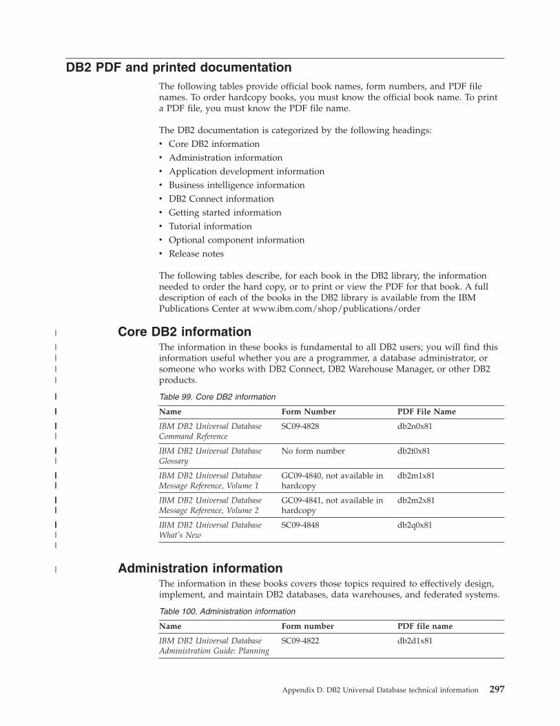
DB2
and
printed
documentation
The
following
tables
provide
official
book
names,
form
numbers,
and
file
names.
To
order
hardcopy
books,
you
must
know
the
official
book
name.
To
a
file,
you
must
know
the
file
name.
The
DB2
documentation
is
categorized
by
the
following
headings:
v
Core
DB2
information
v
Administration
information
v
Application
development
information
v
Business
intelligence
information
v
DB2
Connect
information
v
Getting
started
information
v
Tutorial
information
v
Optional
component
information
v
Release
notes
The
following
tables
describe,
for
each
book
in
the
DB2
library,
the
information
needed
to
order
the
hard
copy,
or
to
or
view
the
for
that
book.
A
full
description
of
each
of
the
books
in
the
DB2
library
is
available
from
the
IBM
Publications
Center
at
www.ibm.com/shop/publications/order
Core
DB2
information
The
information
in
these
books
is
fundamental
to
all
DB2
users;
you
will
find
this
information
useful
whether
you
are
a
programmer,
a
database
administrator,
or
someone
who
works
with
DB2
Connect,
DB2
Warehouse
Manager,
or
other
DB2
products.
Table
99.
Core
DB2
information
Name
Form
Number
File
Name
IBM
DB2
Universal
Database
Command
Reference
SC09-4828
db2n0x81
IBM
DB2
Universal
Database
Glossary
No
form
number
db2t0x81
IBM
DB2
Universal
Database
Message
Reference,
Volume
1
GC09-4840,
not
available
in
hardcopy
db2m1x81
IBM
DB2
Universal
Database
Message
Reference,
Volume
2
GC09-4841,
not
available
in
hardcopy
db2m2x81
IBM
DB2
Universal
Database
What’s
New
SC09-4848
db2q0x81
Administration
information
The
information
in
these
books
covers
those
topics
required
to
effectively
design,
implement,
and
maintain
DB2
databases,
data
warehouses,
and
federated
systems.
Table
100.
Administration
information
Name
Form
number
file
name
IBM
DB2
Universal
Database
Administration
Guide:
Planning
SC09-4822
db2d1x81
Appendix
D.
DB2
Universal
Database
technical
information
297
|
||||
||
|||
||||
||||
|||||
|||||
||||
|
|

Table
100.
Administration
information
(continued)
Name
Form
number
file
name
IBM
DB2
Universal
Database
Administration
Guide:
Implementation
SC09-4820
db2d2x81
IBM
DB2
Universal
Database
Administration
Guide:
Performance
SC09-4821
db2d3x81
IBM
DB2
Universal
Database
Administrative
API
Reference
SC09-4824
db2b0x81
IBM
DB2
Universal
Database
Data
Movement
Utilities
Guide
and
Reference
SC09-4830
db2dmx81
IBM
DB2
Universal
Database
Data
Recovery
and
High
Availability
Guide
and
Reference
SC09-4831
db2hax81
IBM
DB2
Universal
Database
Data
Warehouse
Center
Administration
Guide
SC27-1123
db2ddx81
IBM
DB2
Universal
Database
SQL
Reference,
Volume
1
SC09-4844
db2s1x81
IBM
DB2
Universal
Database
SQL
Reference,
Volume
2
SC09-4845
db2s2x81
IBM
DB2
Universal
Database
System
Monitor
Guide
and
Reference
SC09-4847
db2f0x81
Application
development
information
The
information
in
these
books
is
of
special
interest
to
application
developers
or
programmers
working
with
DB2
Universal
Database
(DB2
UDB).
You
will
find
information
about
supported
languages
and
compilers,
as
well
as
the
documentation
required
to
access
DB2
UDB
using
the
various
supported
programming
interfaces,
such
as
embedded
SQL,
ODBC,
JDBC,
SQLJ,
and
CLI.
If
you
are
using
the
DB2
Information
Center,
you
can
also
access
HTML
versions
of
the
source
code
for
the
sample
programs.
Table
101.
Application
development
information
Name
Form
number
file
name
IBM
DB2
Universal
Database
Application
Development
Guide:
Building
and
Running
Applications
SC09-4825
db2axx81
IBM
DB2
Universal
Database
Application
Development
Guide:
Programming
Client
Applications
SC09-4826
db2a1x81
IBM
DB2
Universal
Database
Application
Development
Guide:
Programming
Server
Applications
SC09-4827
db2a2x81
IBM
DB2
Universal
Database
Call
Level
Interface
Guide
and
Reference,
Volume
1
SC09-4849
db2l1x81
298
Administration
Guide:
Planning

Table
101.
Application
development
information
(continued)
Name
Form
number
file
name
IBM
DB2
Universal
Database
Call
Level
Interface
Guide
and
Reference,
Volume
2
SC09-4850
db2l2x81
IBM
DB2
Universal
Database
Data
Warehouse
Center
Application
Integration
Guide
SC27-1124
db2adx81
IBM
DB2
XML
Extender
Administration
and
Programming
SC27-1234
db2sxx81
Business
intelligence
information
The
information
in
these
books
describes
how
to
use
components
that
enhance
the
data
warehousing
and
analytical
capabilities
of
DB2
Universal
Database.
Table
102.
Business
intelligence
information
Name
Form
number
file
name
IBM
DB2
Warehouse
Manager
Standard
Edition
Information
Catalog
Center
Administration
Guide
SC27-1125
db2dix81
IBM
DB2
Warehouse
Manager
Standard
Edition
Installation
Guide
GC27-1122
db2idx81
IBM
DB2
Warehouse
Manager
Standard
Edition
Managing
ETI
Solution
Conversion
Programs
with
DB2
Warehouse
Manager
SC18-7727
iwhe1mstx80
DB2
Connect
information
The
information
in
this
category
describes
how
to
access
data
on
mainframe
and
midrange
servers
using
DB2
Connect
Enterprise
Edition
or
DB2
Connect
Personal
Edition.
Table
103.
DB2
Connect
information
Name
Form
number
file
name
IBM
Connectivity
Supplement
No
form
number
db2h1x81
IBM
DB2
Connect
Quick
Beginnings
for
DB2
Connect
Enterprise
Edition
GC09-4833
db2c6x81
IBM
DB2
Connect
Quick
Beginnings
for
DB2
Connect
Personal
Edition
GC09-4834
db2c1x81
IBM
DB2
Connect
User’s
Guide
SC09-4835
db2c0x81
Getting
started
information
The
information
in
this
category
is
useful
when
you
are
installing
and
configuring
servers,
clients,
and
other
DB2
products.
Appendix
D.
DB2
Universal
Database
technical
information
299

Table
104.
Getting
started
information
Name
Form
number
file
name
IBM
DB2
Universal
Database
Quick
Beginnings
for
DB2
Clients
GC09-4832,
not
available
in
hardcopy
db2itx81
IBM
DB2
Universal
Database
Quick
Beginnings
for
DB2
Servers
GC09-4836
db2isx81
IBM
DB2
Universal
Database
Quick
Beginnings
for
DB2
Personal
Edition
GC09-4838
db2i1x81
IBM
DB2
Universal
Database
Installation
and
Configuration
Supplement
GC09-4837,
not
available
in
hardcopy
db2iyx81
IBM
DB2
Universal
Database
Quick
Beginnings
for
DB2
Data
Links
Manager
GC09-4829
db2z6x81
Tutorial
information
Tutorial
information
introduces
DB2
features
and
teaches
how
to
perform
various
tasks.
Table
105.
Tutorial
information
Name
Form
number
file
name
Business
Intelligence
Tutorial:
Introduction
to
the
Data
Warehouse
No
form
number
db2tux81
Business
Intelligence
Tutorial:
Extended
Lessons
in
Data
Warehousing
No
form
number
db2tax81
Information
Catalog
Center
Tutorial
No
form
number
db2aix81
Video
Central
for
e-business
Tutorial
No
form
number
db2twx81
Visual
Explain
Tutorial
No
form
number
db2tvx81
Optional
component
information
The
information
in
this
category
describes
how
to
work
with
optional
DB2
components.
Table
106.
Optional
component
information
Name
Form
number
file
name
IBM
DB2
Cube
Views
Guide
and
Reference
SC18–7298
db2aax81
IBM
DB2
Query
Patroller
Guide:
Installation,
Administration
and
Usage
Guide
GC09–7658
db2dwx81
IBM
DB2
Spatial
Extender
and
Geodetic
Extender
User’s
Guide
and
Reference
SC27-1226
db2sbx81
300
Administration
Guide:
Planning

Table
106.
Optional
component
information
(continued)
Name
Form
number
file
name
IBM
DB2
Universal
Database
Data
Links
Manager
Administration
Guide
and
Reference
SC27-1221
db2z0x82
DB2
Net
Search
Extender
Administration
and
User’s
Guide
Note:
HTML
for
this
document
is
not
installed
from
the
HTML
documentation
CD.
SH12-6740
N/A
Release
notes
The
release
notes
provide
additional
information
specific
to
your
product’s
release
and
FixPak
level.
The
release
notes
also
provide
summaries
of
the
documentation
updates
incorporated
in
each
release,
update,
and
FixPak.
Table
107.
Release
notes
Name
Form
number
file
name
DB2
Release
Notes
See
note.
See
note.
DB2
Installation
Notes
Available
on
product
CD-ROM
only.
Not
available.
Note:
The
Release
Notes
are
available
in:
v
XHTML
and
Text
format,
on
the
product
CDs
v
format,
on
the
Documentation
CD
In
addition
the
portions
of
the
Release
Notes
that
discuss
Known
Problems
and
Workarounds
and
Incompatibilities
Between
Releases
also
appear
in
the
DB2
Information
Center.
To
view
the
Release
Notes
in
text
format
on
UNIX-based
platforms,
see
the
Release.Notes
file.
This
file
is
located
in
the
DB2DIR/Readme/%L
directory,
where
%L
represents
the
locale
name
and
DB2DIR
represents:
v
For
AIX
operating
systems:
/usr/opt/db2_08_01
v
For
all
other
UNIX-based
operating
systems:
/opt/IBM/db2/V8.1
Related
concepts:
v
“DB2
documentation
and
help”
on
page
285
Related
tasks:
v
“Printing
DB2
books
from
files”
on
page
302
v
“Ordering
printed
DB2
books”
on
page
302
v
“Invoking
contextual
help
from
a
DB2
tool”
on
page
303
Appendix
D.
DB2
Universal
Database
technical
information
301

Printing
DB2
books
from
files
You
can
DB2
books
from
the
files
on
the
DB2
Documentation
CD.
Using
Adobe
Acrobat
Reader,
you
can
either
the
entire
book
or
a
specific
range
of
pages.
Prerequisites:
Ensure
that
you
have
Adobe
Acrobat
Reader
installed.
If
you
need
to
install
Adobe
Acrobat
Reader,
it
is
available
from
the
Adobe
Web
site
at
www.adobe.com
Procedure:
To
a
DB2
book
from
a
file:
1.
Insert
the
DB2
Documentation
CD.
On
UNIX
operating
systems,
mount
the
DB2
Documentation
CD.
Refer
to
your
Quick
Beginnings
book
for
details
on
how
to
mount
a
CD
on
UNIX
operating
systems.
2.
Open
index.htm.
The
file
opens
in
a
browser
window.
3.
Click
on
the
title
of
the
you
want
to
see.
The
will
open
in
Acrobat
Reader.
4.
Select
File
→
to
any
portions
of
the
book
that
you
want.
Related
concepts:
v
“DB2
Information
Center”
on
page
286
Related
tasks:
v
“Mounting
the
CD-ROM
(AIX)”
in
the
Quick
Beginnings
for
DB2
Servers
v
“Mounting
the
CD-ROM
(HP-UX)”
in
the
Quick
Beginnings
for
DB2
Servers
v
“Mounting
the
CD-ROM
(Linux)”
in
the
Quick
Beginnings
for
DB2
Servers
v
“Ordering
printed
DB2
books”
on
page
302
v
“Mounting
the
CD-ROM
(Solaris
Operating
Environment)”
in
the
Quick
Beginnings
for
DB2
Servers
Related
reference:
v
“DB2
and
printed
documentation”
on
page
297
Ordering
printed
DB2
books
If
you
prefer
to
use
hardcopy
books,
you
can
order
them
in
one
of
three
ways.
Procedure:
Printed
books
can
be
ordered
in
some
countries
or
regions.
Check
the
IBM
Publications
website
for
your
country
or
region
to
see
if
this
service
is
available
in
your
country
or
region.
When
the
publications
are
available
for
ordering,
you
can:
v
Contact
your
IBM
authorized
dealer
or
marketing
representative.
To
find
a
local
IBM
representative,
check
the
IBM
Worldwide
Directory
of
Contacts
at
www.ibm.com/planetwide
v
Phone
1-800-879-2755
in
the
United
States
or
1-800-IBM-4YOU
in
Canada.
302
Administration
Guide:
Planning
|||
|||
|
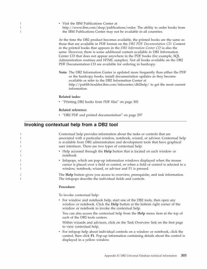
v
Visit
the
IBM
Publications
Center
at
http://www.ibm.com/shop/publications/order.
The
ability
to
order
books
from
the
IBM
Publications
Center
may
not
be
available
in
all
countries.
At
the
time
the
DB2
product
becomes
available,
the
printed
books
are
the
same
as
those
that
are
available
in
format
on
the
DB2
Documentation
CD.
Content
in
the
printed
books
that
appears
in
the
DB2
Information
Center
CD
is
also
the
same.
However,
there
is
some
additional
content
available
in
DB2
Information
Center
CD
that
does
not
appear
anywhere
in
the
books
(for
example,
SQL
Administration
routines
and
HTML
samples).
Not
all
books
available
on
the
DB2
Documentation
CD
are
available
for
ordering
in
hardcopy.
Note:
The
DB2
Information
Center
is
updated
more
frequently
than
either
the
or
the
hardcopy
books;
install
documentation
updates
as
they
become
available
or
refer
to
the
DB2
Information
Center
at
http://publib.boulder.ibm.com/infocenter/db2help/
to
get
the
most
current
information.
Related
tasks:
v
“Printing
DB2
books
from
files”
on
page
302
Related
reference:
v
“DB2
and
printed
documentation”
on
page
297
Invoking
contextual
help
from
a
DB2
tool
Contextual
help
provides
information
about
the
tasks
or
controls
that
are
associated
with
a
particular
window,
notebook,
wizard,
or
advisor.
Contextual
help
is
available
from
DB2
administration
and
development
tools
that
have
graphical
user
interfaces.
There
are
two
types
of
contextual
help:
v
Help
accessed
through
the
Help
button
that
is
located
on
each
window
or
notebook
v
Infopops,
which
are
pop-up
information
windows
displayed
when
the
mouse
cursor
is
placed
over
a
field
or
control,
or
when
a
field
or
control
is
selected
in
a
window,
notebook,
wizard,
or
advisor
and
F1
is
pressed.
The
Help
button
gives
you
access
to
overview,
prerequisite,
and
task
information.
The
infopops
describe
the
individual
fields
and
controls.
Procedure:
To
invoke
contextual
help:
v
For
window
and
notebook
help,
start
one
of
the
DB2
tools,
then
open
any
window
or
notebook.
Click
the
Help
button
at
the
bottom
right
corner
of
the
window
or
notebook
to
invoke
the
contextual
help.
You
can
also
access
the
contextual
help
from
the
Help
menu
item
at
the
top
of
each
of
the
DB2
tools
centers.
Within
wizards
and
advisors,
click
on
the
Task
Overview
link
on
the
first
page
to
view
contextual
help.
v
For
infopop
help
about
individual
controls
on
a
window
or
notebook,
click
the
control,
then
click
F1.
Pop-up
information
containing
details
about
the
control
is
displayed
in
a
yellow
window.
Appendix
D.
DB2
Universal
Database
technical
information
303
|||
||||
||
|||
||

Note:
To
display
infopops
simply
by
holding
the
mouse
cursor
over
a
field
or
control,
select
the
Automatically
display
infopops
check
box
on
the
Documentation
page
of
the
Tool
Settings
notebook.
Similar
to
infopops,
diagnosis
pop-up
information
is
another
form
of
context-sensitive
help;
they
contain
data
entry
rules.
Diagnosis
pop-up
information
is
displayed
in
a
purple
window
that
appears
when
data
that
is
not
valid
or
that
is
insufficient
is
entered.
Diagnosis
pop-up
information
can
appear
for:
–
Compulsory
fields.
–
Fields
whose
data
follows
a
precise
format,
such
as
a
date
field.
Related
tasks:
v
“Invoking
the
DB2
Information
Center”
on
page
294
v
“Invoking
message
help
from
the
command
line
processor”
on
page
304
v
“Invoking
command
help
from
the
command
line
processor”
on
page
304
v
“Invoking
SQL
state
help
from
the
command
line
processor”
on
page
305
v
“How
to
use
the
DB2
UDB
help:
Common
GUI
help”
Invoking
message
help
from
the
command
line
processor
Message
help
describes
the
cause
of
a
message
and
describes
any
action
you
should
take
in
response
to
the
error.
Procedure:
To
invoke
message
help,
open
the
command
line
processor
and
enter:
?
XXXnnnnn
where
XXXnnnnn
represents
a
valid
message
identifier.
For
example,
?
SQL30081
displays
help
about
the
SQL30081
message.
Related
concepts:
v
“Introduction
to
messages”
in
the
Message
Reference
Volume
1
Related
reference:
v
“db2
-
Command
Line
Processor
Invocation
Command”
in
the
Command
Reference
Invoking
command
help
from
the
command
line
processor
Command
help
explains
the
syntax
of
commands
in
the
command
line
processor.
Procedure:
To
invoke
command
help,
open
the
command
line
processor
and
enter:
?
command
where
command
represents
a
keyword
or
the
entire
command.
For
example,
?
catalog
displays
help
for
all
of
the
CATALOG
commands,
while
?
catalog
database
displays
help
only
for
the
CATALOG
DATABASE
command.
304
Administration
Guide:
Planning
|||||
|
|
|
||
|
|
|
|
|
|
|
|
||
|
|
|
|
|
|
||

Related
tasks:
v
“Invoking
contextual
help
from
a
DB2
tool”
on
page
303
v
“Invoking
the
DB2
Information
Center”
on
page
294
v
“Invoking
message
help
from
the
command
line
processor”
on
page
304
v
“Invoking
SQL
state
help
from
the
command
line
processor”
on
page
305
Related
reference:
v
“db2
-
Command
Line
Processor
Invocation
Command”
in
the
Command
Reference
Invoking
SQL
state
help
from
the
command
line
processor
DB2
Univerrsal
Database
returns
an
SQLSTATE
value
for
conditions
that
could
be
the
result
of
an
SQL
statement.
SQLSTATE
help
explains
the
meanings
of
SQL
states
and
SQL
state
class
codes.
Procedure:
To
invoke
SQL
state
help,
open
the
command
line
processor
and
enter:
?
sqlstate
or
?
class
code
where
sqlstate
represents
a
valid
five-digit
SQL
state
and
class
code
represents
the
first
two
digits
of
the
SQL
state.
For
example,
?
08003
displays
help
for
the
08003
SQL
state,
and
?
08
displays
help
for
the
08
class
code.
Related
tasks:
v
“Invoking
the
DB2
Information
Center”
on
page
294
v
“Invoking
message
help
from
the
command
line
processor”
on
page
304
v
“Invoking
command
help
from
the
command
line
processor”
on
page
304
DB2
tutorials
The
DB2®
tutorials
help
you
learn
about
various
aspects
of
DB2
Universal
Database.
The
tutorials
provide
lessons
with
step-by-step
instructions
in
the
areas
of
developing
applications,
tuning
SQL
query
performance,
working
with
data
warehouses,
managing
metadata,
and
developing
Web
services
using
DB2.
Before
you
begin:
You
can
view
the
XHTML
versions
of
the
tutorials
from
the
Information
Center
at
http://publib.boulder.ibm.com/infocenter/db2help/.
Some
tutorial
lessons
use
sample
data
or
code.
See
each
tutorial
for
a
description
of
any
prerequisites
for
its
specific
tasks.
DB2
Universal
Database
tutorials:
Click
on
a
tutorial
title
in
the
following
list
to
view
that
tutorial.
Appendix
D.
DB2
Universal
Database
technical
information
305
|
|
|
|
|
|
||
|
|||
|
|
|
||
||
|
|
|
|

Business
Intelligence
Tutorial:
Introduction
to
the
Data
Warehouse
Center
Perform
introductory
data
warehousing
tasks
using
the
Data
Warehouse
Center.
Business
Intelligence
Tutorial:
Extended
Lessons
in
Data
Warehousing
Perform
advanced
data
warehousing
tasks
using
the
Data
Warehouse
Center.
Information
Catalog
Center
Tutorial
Create
and
manage
an
information
catalog
to
locate
and
use
metadata
using
the
Information
Catalog
Center.
Visual
Explain
Tutorial
Analyze,
optimize,
and
tune
SQL
statements
for
better
performance
using
Visual
Explain.
DB2
troubleshooting
information
A
wide
variety
of
troubleshooting
and
problem
determination
information
is
available
to
assist
you
in
using
DB2®
products.
DB2
documentation
Troubleshooting
information
can
be
found
throughout
the
DB2
Information
Center,
as
well
as
throughout
the
books
that
make
up
the
DB2
library.
You
can
refer
to
the
″Support
and
troubleshooting″
branch
of
the
DB2
Information
Center
navigation
tree
(in
the
left
pane
of
your
browser
window)
to
see
a
complete
listing
of
the
DB2
troubleshooting
documentation.
DB2
Technical
Support
Web
site
Refer
to
the
DB2
Technical
Support
Web
site
if
you
are
experiencing
problems
and
want
help
finding
possible
causes
and
solutions.
The
Technical
Support
site
has
links
to
the
latest
DB2
publications,
TechNotes,
Authorized
Program
Analysis
Reports
(APARs),
FixPaks
and
the
latest
listing
of
internal
DB2
error
codes,
and
other
resources.
You
can
search
through
this
knowledge
base
to
find
possible
solutions
to
your
problems.
Access
the
DB2
Technical
Support
Web
site
at
http://www.ibm.com/software/data/db2/udb/winos2unix/support
DB2
Problem
Determination
Tutorial
Series
Refer
to
the
DB2
Problem
Determination
Tutorial
Series
Web
site
to
find
information
on
how
to
quickly
identify
and
resolve
problems
you
might
encounter
while
working
with
DB2
products.
One
tutorial
introduces
you
to
the
DB2
problem
determination
facilities
and
tools
available,
and
helps
you
decide
when
to
use
them.
Other
tutorials
deal
with
related
topics,
such
as
″Database
Engine
Problem
Determination″,
″Performance
Problem
Determination″,
and
″Application
Problem
Determination″.
See
the
full
set
of
DB2
problem
determination
tutorials
on
the
DB2
Technical
Support
site
at
http://www.ibm.com/software/data/support/pdm/db2tutorials.html
Related
concepts:
v
“DB2
Information
Center”
on
page
286
v
“Introduction
to
problem
determination
-
DB2
Technical
Support
tutorial”
in
the
Troubleshooting
Guide
306
Administration
Guide:
Planning

Accessibility
Accessibility
features
help
users
with
physical
disabilities,
such
as
restricted
mobility
or
limited
vision,
to
use
software
products
successfully.
The
following
list
specifies
the
major
accessibility
features
in
DB2®
Version
8
products:
v
All
DB2
functionality
is
available
using
the
keyboard
for
navigation
instead
of
the
mouse.
For
more
information,
see
“Keyboard
input
and
navigation.”
v
You
can
customize
the
size
and
color
of
the
fonts
on
DB2
user
interfaces.
For
more
information,
see
“Accessible
display.”
v
DB2
products
support
accessibility
applications
that
use
the
Java™
Accessibility
API.
For
more
information,
see
“Compatibility
with
assistive
technologies”
on
page
308.
v
DB2
documentation
is
provided
in
an
accessible
format.
For
more
information,
see
“Accessible
documentation”
on
page
308.
Keyboard
input
and
navigation
Keyboard
input
You
can
operate
the
DB2
tools
using
only
the
keyboard.
You
can
use
keys
or
key
combinations
to
perform
operations
that
can
also
be
done
using
a
mouse.
Standard
operating
system
keystrokes
are
used
for
standard
operating
system
operations.
For
more
information
about
using
keys
or
key
combinations
to
perform
operations,
see
Keyboard
shortcuts
and
accelerators:
Common
GUI
help.
Keyboard
navigation
You
can
navigate
the
DB2
tools
user
interface
using
keys
or
key
combinations.
For
more
information
about
using
keys
or
key
combinations
to
navigate
the
DB2
Tools,
see
Keyboard
shortcuts
and
accelerators:
Common
GUI
help.
Keyboard
focus
In
UNIX®
operating
systems,
the
area
of
the
active
window
where
your
keystrokes
will
have
an
effect
is
highlighted.
Accessible
display
The
DB2
tools
have
features
that
improve
accessibility
for
users
with
low
vision
or
other
visual
impairments.
These
accessibility
enhancements
include
support
for
customizable
font
properties.
Font
settings
You
can
select
the
color,
size,
and
font
for
the
text
in
menus
and
dialog
windows,
using
the
Tools
Settings
notebook.
For
more
information
about
specifying
font
settings,
see
Changing
the
fonts
for
menus
and
text:
Common
GUI
help.
Non-dependence
on
color
You
do
not
need
to
distinguish
between
colors
in
order
to
use
any
of
the
functions
in
this
product.
Appendix
D.
DB2
Universal
Database
technical
information
307
||||
||

Compatibility
with
assistive
technologies
The
DB2
tools
interfaces
support
the
Java
Accessibility
API,
which
enables
you
to
use
screen
readers
and
other
assistive
technologies
with
DB2
products.
Accessible
documentation
Documentation
for
DB2
is
provided
in
XHTML
1.0
format,
which
is
viewable
in
most
Web
browsers.
XHTML
allows
you
to
view
documentation
according
to
the
display
preferences
set
in
your
browser.
It
also
allows
you
to
use
screen
readers
and
other
assistive
technologies.
Syntax
diagrams
are
provided
in
dotted
decimal
format.
This
format
is
available
only
if
you
are
accessing
the
online
documentation
using
a
screen-reader.
Related
concepts:
v
“Dotted
decimal
syntax
diagrams”
on
page
308
Dotted
decimal
syntax
diagrams
Syntax
diagrams
are
provided
in
dotted
decimal
format
for
users
accessing
the
Information
Center
using
a
screen
reader.
In
dotted
decimal
format,
each
syntax
element
is
written
on
a
separate
line.
If
two
or
more
syntax
elements
are
always
present
together
(or
always
absent
together),
they
can
appear
on
the
same
line,
because
they
can
be
considered
as
a
single
compound
syntax
element.
Each
line
starts
with
a
dotted
decimal
number;
for
example,
3
or
3.1
or
3.1.1.
To
hear
these
numbers
correctly,
make
sure
that
your
screen
reader
is
set
to
read
out
punctuation.
All
the
syntax
elements
that
have
the
same
dotted
decimal
number
(for
example,
all
the
syntax
elements
that
have
the
number
3.1)
are
mutually
exclusive
alternatives.
If
you
hear
the
lines
3.1
USERID
and
3.1
SYSTEMID,
you
know
that
your
syntax
can
include
either
USERID
or
SYSTEMID,
but
not
both.
The
dotted
decimal
numbering
level
denotes
the
level
of
nesting.
For
example,
if
a
syntax
element
with
dotted
decimal
number
3
is
followed
by
a
series
of
syntax
elements
with
dotted
decimal
number
3.1,
all
the
syntax
elements
numbered
3.1
are
subordinate
to
the
syntax
element
numbered
3.
Certain
words
and
symbols
are
used
next
to
the
dotted
decimal
numbers
to
add
information
about
the
syntax
elements.
Occasionally,
these
words
and
symbols
might
occur
at
the
beginning
of
the
element
itself.
For
ease
of
identification,
if
the
word
or
symbol
is
a
part
of
the
syntax
element,
it
is
preceded
by
the
backslash
(\)
character.
The
*
symbol
can
be
used
next
to
a
dotted
decimal
number
to
indicate
that
the
syntax
element
repeats.
For
example,
syntax
element
*FILE
with
dotted
decimal
number
3
is
given
the
format
3
\*
FILE.
Format
3*
FILE
indicates
that
syntax
element
FILE
repeats.
Format
3*
\*
FILE
indicates
that
syntax
element
*
FILE
repeats.
Characters
such
as
commas,
which
are
used
to
separate
a
string
of
syntax
elements,
are
shown
in
the
syntax
just
before
the
items
they
separate.
These
characters
can
appear
on
the
same
line
as
each
item,
or
on
a
separate
line
with
the
same
dotted
decimal
number
as
the
relevant
items.
The
line
can
also
show
another
symbol
giving
information
about
the
syntax
elements.
For
example,
the
lines
5.1*,
5.1
LASTRUN,
and
5.1
DELETE
mean
that
if
you
use
more
than
one
of
the
308
Administration
Guide:
Planning
|
||
||||
||||||
||||
|||||||||
||||||

LASTRUN
and
DELETE
syntax
elements,
the
elements
must
be
separated
by
a
comma.
If
no
separator
is
given,
assume
that
you
use
a
blank
to
separate
each
syntax
element.
If
a
syntax
element
is
preceded
by
the
%
symbol,
this
indicates
a
reference
that
is
defined
elsewhere.
The
string
following
the
%
symbol
is
the
name
of
a
syntax
fragment
rather
than
a
literal.
For
example,
the
line
2.1
%OP1
means
that
you
should
refer
to
separate
syntax
fragment
OP1.
The
following
words
and
symbols
are
used
next
to
the
dotted
decimal
numbers:
v
?
means
an
optional
syntax
element.
A
dotted
decimal
number
followed
by
the
?
symbol
indicates
that
all
the
syntax
elements
with
a
corresponding
dotted
decimal
number,
and
any
subordinate
syntax
elements,
are
optional.
If
there
is
only
one
syntax
element
with
a
dotted
decimal
number,
the
?
symbol
is
displayed
on
the
same
line
as
the
syntax
element,
(for
example
5?
NOTIFY).
If
there
is
more
than
one
syntax
element
with
a
dotted
decimal
number,
the
?
symbol
is
displayed
on
a
line
by
itself,
followed
by
the
syntax
elements
that
are
optional.
For
example,
if
you
hear
the
lines
5
?,
5
NOTIFY,
and
5
UPDATE,
you
know
that
syntax
elements
NOTIFY
and
UPDATE
are
optional;
that
is,
you
can
choose
one
or
none
of
them.
The
?
symbol
is
equivalent
to
a
bypass
line
in
a
railroad
diagram.
v
!
means
a
default
syntax
element.
A
dotted
decimal
number
followed
by
the
!
symbol
and
a
syntax
element
indicates
that
the
syntax
element
is
the
default
option
for
all
syntax
elements
that
share
the
same
dotted
decimal
number.
Only
one
of
the
syntax
elements
that
share
the
same
dotted
decimal
number
can
specify
a
!
symbol.
For
example,
if
you
hear
the
lines
2?
FILE,
2.1!
(KEEP),
and
2.1
(DELETE),
you
know
that
(KEEP)
is
the
default
option
for
the
FILE
keyword.
In
this
example,
if
you
include
the
FILE
keyword
but
do
not
specify
an
option,
default
option
KEEP
will
be
applied.
A
default
option
also
applies
to
the
next
higher
dotted
decimal
number.
In
this
example,
if
the
FILE
keyword
is
omitted,
default
FILE(KEEP)
is
used.
However,
if
you
hear
the
lines
2?
FILE,
2.1,
2.1.1!
(KEEP),
and
2.1.1
(DELETE),
the
default
option
KEEP
only
applies
to
the
next
higher
dotted
decimal
number,
2.1
(which
does
not
have
an
associated
keyword),
and
does
not
apply
to
2?
FILE.
Nothing
is
used
if
the
keyword
FILE
is
omitted.
v
*
means
a
syntax
element
that
can
be
repeated
0
or
more
times.
A
dotted
decimal
number
followed
by
the
*
symbol
indicates
that
this
syntax
element
can
be
used
zero
or
more
times;
that
is,
it
is
optional
and
can
be
repeated.
For
example,
if
you
hear
the
line
5.1*
data
area,
you
know
that
you
can
include
one
data
area,
more
than
one
data
area,
or
no
data
area.
If
you
hear
the
lines
3*,
3
HOST,
and
3
STATE,
you
know
that
you
can
include
HOST,
STATE,
both
together,
or
nothing.
Notes:
1.
If
a
dotted
decimal
number
has
an
asterisk
(*)
next
to
it
and
there
is
only
one
item
with
that
dotted
decimal
number,
you
can
repeat
that
same
item
more
than
once.
2.
If
a
dotted
decimal
number
has
an
asterisk
next
to
it
and
several
items
have
that
dotted
decimal
number,
you
can
use
more
than
one
item
from
the
list,
but
you
cannot
use
the
items
more
than
once
each.
In
the
previous
example,
you
could
write
HOST
STATE,
but
you
could
not
write
HOST
HOST.
3.
The
*
symbol
is
equivalent
to
a
loop-back
line
in
a
railroad
syntax
diagram.v
+
means
a
syntax
element
that
must
be
included
one
or
more
times.
A
dotted
decimal
number
followed
by
the
+
symbol
indicates
that
this
syntax
element
must
be
included
one
or
more
times;
that
is,
it
must
be
included
at
least
once
Appendix
D.
DB2
Universal
Database
technical
information
309
|||
||||
|
|||||||||||
||||||||||||||
|||||||
|
|||
||||
|
|||

and
can
be
repeated.
For
example,
if
you
hear
the
line
6.1+
data
area,
you
must
include
at
least
one
data
area.
If
you
hear
the
lines
2+,
2
HOST,
and
2
STATE,
you
know
that
you
must
include
HOST,
STATE,
or
both.
Similar
to
the
*
symbol,
the
+
symbol
can
only
repeat
a
particular
item
if
it
is
the
only
item
with
that
dotted
decimal
number.
The
+
symbol,
like
the
*
symbol,
is
equivalent
to
a
loop-back
line
in
a
railroad
syntax
diagram.
Related
concepts:
v
“Accessibility”
on
page
307
Related
tasks:
v
“Contents
:
Common
help”
Related
reference:
v
“How
to
read
the
syntax
diagrams”
in
the
SQL
Reference,
Volume
2
Common
Criteria
certification
of
DB2
Universal
Database
products
DB2
Universal
Database
is
being
evaluated
for
certification
under
the
Common
Criteria
at
evaluation
assurance
level
4
(EAL4).
For
more
information
about
Common
Criteria,
see
the
Common
Criteria
web
site
at:
http://niap.nist.gov/cc-scheme/.
310
Administration
Guide:
Planning
||||||
|
|
|
|
|
|
|
||||

Appendix
E.
Notices
IBM
may
not
offer
the
products,
services,
or
features
discussed
in
this
document
in
all
countries.
Consult
your
local
IBM
representative
for
information
on
the
products
and
services
currently
available
in
your
area.
Any
reference
to
an
IBM
product,
program,
or
service
is
not
intended
to
state
or
imply
that
only
that
IBM
product,
program,
or
service
may
be
used.
Any
functionally
equivalent
product,
program,
or
service
that
does
not
infringe
any
IBM
intellectual
property
right
may
be
used
instead.
However,
it
is
the
user’s
responsibility
to
evaluate
and
verify
the
operation
of
any
non-IBM
product,
program,
or
service.
IBM
may
have
patents
or
pending
patent
applications
covering
subject
matter
described
in
this
document.
The
furnishing
of
this
document
does
not
give
you
any
license
to
these
patents.
You
can
send
license
inquiries,
in
writing,
to:
IBM
Director
of
Licensing
IBM
Corporation
North
Castle
Drive
Armonk,
NY
10504-1785
U.S.A.
For
license
inquiries
regarding
double-byte
(DBCS)
information,
contact
the
IBM
Intellectual
Property
Department
in
your
country/region
or
send
inquiries,
in
writing,
to:
IBM
World
Trade
Asia
Corporation
Licensing
2-31
Roppongi
3-chome,
Minato-ku
Tokyo
106,
Japan
The
following
paragraph
does
not
apply
to
the
United
Kingdom
or
any
other
country/region
where
such
provisions
are
inconsistent
with
local
law:
INTERNATIONAL
BUSINESS
MACHINES
CORPORATION
PROVIDES
THIS
PUBLICATION
“AS
IS”
WITHOUT
WARRANTY
OF
ANY
KIND,
EITHER
EXPRESS
OR
IMPLIED,
INCLUDING,
BUT
NOT
LIMITED
TO,
THE
IMPLIED
WARRANTIES
OF
NON-INFRINGEMENT,
MERCHANTABILITY,
OR
FITNESS
FOR
A
PARTICULAR
PURPOSE.
Some
states
do
not
allow
disclaimer
of
express
or
implied
warranties
in
certain
transactions;
therefore,
this
statement
may
not
apply
to
you.
This
information
could
include
technical
inaccuracies
or
typographical
errors.
Changes
are
periodically
made
to
the
information
herein;
these
changes
will
be
incorporated
in
new
editions
of
the
publication.
IBM
may
make
improvements
and/or
changes
in
the
product(s)
and/or
the
program(s)
described
in
this
publication
at
any
time
without
notice.
Any
references
in
this
information
to
non-IBM
Web
sites
are
provided
for
convenience
only
and
do
not
in
any
manner
serve
as
an
endorsement
of
those
Web
sites.
The
materials
at
those
Web
sites
are
not
part
of
the
materials
for
this
IBM
product,
and
use
of
those
Web
sites
is
at
your
own
risk.
IBM
may
use
or
distribute
any
of
the
information
you
supply
in
any
way
it
believes
appropriate
without
incurring
any
obligation
to
you.
©
Copyright
IBM
Corp.
1993
-
2004
311

Licensees
of
this
program
who
wish
to
have
information
about
it
for
the
purpose
of
enabling:
(i)
the
exchange
of
information
between
independently
created
programs
and
other
programs
(including
this
one)
and
(ii)
the
mutual
use
of
the
information
that
has
been
exchanged,
should
contact:
IBM
Canada
Limited
Office
of
the
Lab
Director
8200
Warden
Avenue
Markham,
Ontario
L6G
1C7
CANADA
Such
information
may
be
available,
subject
to
appropriate
terms
and
conditions,
including
in
some
cases
payment
of
a
fee.
The
licensed
program
described
in
this
document
and
all
licensed
material
available
for
it
are
provided
by
IBM
under
terms
of
the
IBM
Customer
Agreement,
IBM
International
Program
License
Agreement,
or
any
equivalent
agreement
between
us.
Any
performance
data
contained
herein
was
determined
in
a
controlled
environment.
Therefore,
the
results
obtained
in
other
operating
environments
may
vary
significantly.
Some
measurements
may
have
been
made
on
development-level
systems,
and
there
is
no
guarantee
that
these
measurements
will
be
the
same
on
generally
available
systems.
Furthermore,
some
measurements
may
have
been
estimated
through
extrapolation.
Actual
results
may
vary.
Users
of
this
document
should
verify
the
applicable
data
for
their
specific
environment.
Information
concerning
non-IBM
products
was
obtained
from
the
suppliers
of
those
products,
their
published
announcements,
or
other
publicly
available
sources.
IBM
has
not
tested
those
products
and
cannot
confirm
the
accuracy
of
performance,
compatibility,
or
any
other
claims
related
to
non-IBM
products.
Questions
on
the
capabilities
of
non-IBM
products
should
be
addressed
to
the
suppliers
of
those
products.
All
statements
regarding
IBM’s
future
direction
or
intent
are
subject
to
change
or
withdrawal
without
notice,
and
represent
goals
and
objectives
only.
This
information
may
contain
examples
of
data
and
reports
used
in
daily
business
operations.
To
illustrate
them
as
completely
as
possible,
the
examples
include
the
names
of
individuals,
companies,
brands,
and
products.
All
of
these
names
are
fictitious,
and
any
similarity
to
the
names
and
addresses
used
by
an
actual
business
enterprise
is
entirely
coincidental.
COPYRIGHT
LICENSE:
This
information
may
contain
sample
application
programs,
in
source
language,
which
illustrate
programming
techniques
on
various
operating
platforms.
You
may
copy,
modify,
and
distribute
these
sample
programs
in
any
form
without
payment
to
IBM
for
the
purposes
of
developing,
using,
marketing,
or
distributing
application
programs
conforming
to
the
application
programming
interface
for
the
operating
platform
for
which
the
sample
programs
are
written.
These
examples
have
not
been
thoroughly
tested
under
all
conditions.
IBM,
therefore,
cannot
guarantee
or
imply
reliability,
serviceability,
or
function
of
these
programs.
Each
copy
or
any
portion
of
these
sample
programs
or
any
derivative
work
must
include
a
copyright
notice
as
follows:
312
Administration
Guide:
Planning

©
(your
company
name)
(year).
Portions
of
this
code
are
derived
from
IBM
Corp.
Sample
Programs.
©
Copyright
IBM
Corp.
_enter
the
year
or
years_.
All
rights
reserved.
Trademarks
The
following
terms
are
trademarks
of
International
Business
Machines
Corporation
in
the
United
States,
other
countries,
or
both,
and
have
been
used
in
at
least
one
of
the
documents
in
the
DB2
UDB
documentation
library.
ACF/VTAM
AISPO
AIX
AIXwindows
AnyNet
APPN
AS/400
BookManager
C
Set++
C/370
CICS
Database
2
DataHub
DataJoiner
DataPropagator
DataRefresher
DB2
DB2
Connect
DB2
Extenders
DB2
OLAP
Server
DB2
Information
Integrator
DB2
Query
Patroller
DB2
Universal
Database
Distributed
Relational
Database
Architecture
DRDA
eServer
Extended
Services
FFST
First
Failure
Support
Technology
IBM
IMS
IMS/ESA
iSeries
LAN
Distance
MVS
MVS/ESA
MVS/XA
Net.Data
NetView
OS/390
OS/400
PowerPC
pSeries
QBIC
QMF
RACF
RISC
System/6000
RS/6000
S/370
SP
SQL/400
SQL/DS
System/370
System/390
SystemView
Tivoli
VisualAge
VM/ESA
VSE/ESA
VTAM
WebExplorer
WebSphere
WIN-OS/2
z/OS
zSeries
The
following
terms
are
trademarks
or
registered
trademarks
of
other
companies
and
have
been
used
in
at
least
one
of
the
documents
in
the
DB2
UDB
documentation
library:
Microsoft,
Windows,
Windows
NT,
and
the
Windows
logo
are
trademarks
of
Microsoft
Corporation
in
the
United
States,
other
countries,
or
both.
Intel
and
Pentium
are
trademarks
of
Intel
Corporation
in
the
United
States,
other
countries,
or
both.
Java
and
all
Java-based
trademarks
are
trademarks
of
Sun
Microsystems,
Inc.
in
the
United
States,
other
countries,
or
both.
Appendix
E.
Notices
313

UNIX
is
a
registered
trademark
of
The
Open
Group
in
the
United
States
and
other
countries.
Other
company,
product,
or
service
names
may
be
trademarks
or
service
marks
of
others.
314
Administration
Guide:
Planning

Index
Aaccessibility
dotted
decimal
syntax
diagrams
308
features
307
agentsdata
warehouse
43
described
47
AIXlarge
page
support
283
system
commandsvmo
283
vmtune
283
append
mode
tables
132
application
designcollating
sequences,
guidelines
268
applicationsincompatibility
207
audit
activities
69
audit
context
recordsincompatibility
207
authenticationdescription
25
authorityincompatibility
207
authorizationdatabase
design
considerations
69
description
25
automatic
client
reroute
183
automatic
maintenance
18
backup
15
Bbackup
automatic
18
backupsautomated
15
BEA
Tuxedo,
configuring
200
bidirectional
CCSID
supportDB2
262
DB2
Connect
266
list
of
CCSIDs
263
block
indexes
137
buffer
poolsdescription
3
IBMDEFAULTBP
114
business
rulesdescription
12
transitional
68
CCALL
statementincompatibility
207
capacityfor
each
environment
34
casting
FOR
BIT
DATAincompatibility
207
catalog
table
spaces
89,
128
CCSID
(coded
character
set
identifier)
280,
281
bidirectional
supportDB2
262
DB2
Connect
266
types
listed
263
CHAR
functionincompatibility
207
character
stringsUnicode
276
check
constraintsas
business
rules
12
check
pending
state
63
choosingextent
size
113
multidimensional
table
dimensions
153
table
spaces
89
CHR
functionincompatibility
207
client
rerouteautomatic
183
clustering,
data
137
code
page
950IBM
and
Microsoft
differences
231
code
page
conversionincompatibility
207
code
pages923
and
924
252,
260
converting
1394
to
Unicode,
previous
conversion
tables
280
converting
Shift
JIS
X0213
to
Unicode,
previous
conversion
tables
280
DB2
supported
231
with
euro
symbol
252,
253
code
point
268,
280
code
setsDB2
supported
231
coded
character
set
identifier
943considerations
when
using
280
collating
algorithm
differencesThai
and
Unicode
274
collating
sequencescode
point
268
concerns,
general
268
identity
sequence
268
multi-byte
characters
268
overview
268
Thai
characters
269
Unicode
274
collocation,
table
87
column
expressions,
multidimensional
tables
160
columnsdefining
for
a
table
55
command
helpinvoking
304
commiterrors
during
two-phase
176
two-phase
174
compatibilitypartition
87
composite
block
indexes
137
composite
keysprimary
keys
56
configuration
filesdescription
11
location
11
configuration
parametersDB2
transaction
manager
considerations
171
description
11
incompatibility
207
configurationsmultiple
partition
34
configure
automatic
maintenance
wizard
18
connection
failureautomatic
client
reroute
183
constantsUnicode
278
constraintscheck
12
foreign
key
12
informational
12,
63
NOT
NULL
12
primary
key
12
referential
63
table
check
63
unique
12,
63
containersdescription
3
DMS
table
spacesaddition
of
containers
to
98
dropping
containers
from
106
extension
of
containers
in
98
reduction
of
containers
in
106
CONTROL
privilege
on
packagesincompatibility
207
conversionsUnicode
to
CCSID
943
280,
281
coordinator
node
29
CREATE
TABLEOVERFLOW
clause
136
creatingmultidimensional
tables
160
Unicode
databases
278
Ddata
large
object
(LOB)
77
long
field
76
partitioning
29
data
typesdatabase
design
considerations
69
Unicode
handling
276
data
types
and
scrollable
cursorsincompatibility
207
data
warehouse
objects
43
©
Copyright
IBM
Corp.
1993
-
2004
315

data
warehousingdefined
43
informational
data
43
operational
data
43
database
connectionincompatibility
207
database
designadditional
considerations
69
logical
51
physical
71
database
directoriesstructure
described
71
database
objectsdatabase
partition
groups
3
databases
3
indexes
3
instances
3
recovery
history
file
15
recovery
log
file
15
schemas
3
system
catalog
tables
3
table
space
change
history
file
15
table
spaces
3
tables
3
views
3
database
partition
groupscollocation
83
description
3,
81
designing
83
determining
data
location
84
IBMCATGROUP
89
IBMDEFAULTGROUP
89
IBMTEMPGROUP
89
database
partitionsand
multidimensional
clustering
137
description
29
database-managed
space
(DMS)containers
98
description
94
overview
3
reducing
containers
106
databasesaccessing
in
a
single
transaction
168
description
3
distributed
26
estimating
size
requirements
73
host
system
168
language,
selecting
261
nonrecoverable
15
recoverable
15
datesformats
270
DB2
booksprinting
files
302
DB2
Connectfor
multisite
updates
168
incompatibility
207
DB2
Information
Center
286
invoking
294
DB2
sync
point
manager
(SPM)
173
DB2
transaction
manager
170
DB2
tutorials
305
DB2_LIKE_VARCHARincompatibility
207
DB2_NO_MPFA_FOR
_NEW_DB
92,
113,
160
DB2_PARALLEL_IO
registry
variable
129
DB2_SMS_TRUNC
_TMPTABLE_THRESH
81
DB2_SMS_TRUNC_TMPTABLE
_THRESH
127
DB2_USE_PAGE_CONTAINER_TAG
environment
variable
129
db2empfa
utility
92,
113,
160
declusteringpartial
29
definingcolumns
55
delete
rulewith
referential
constraint
63
dependent
row
63
dependent
table
63
descendent
row
63
descendent
table
63
DESCRIBE
statement
outputincompatibility
207
design
advisormultidemensional
clustering
137
designingdatabase
partition
groups
83
tables
spaces
89
dimension
block
indexes
137
dimensionsmultidimensional
tables
137,
153
disability
307
disablingeuro
symbol
support
252,
253
disaster
recoveryhigh
availability
feature
23
distributed
relational
databasesunits
of
work
26
distributed
transaction
processingapplication
program
179
configuration
considerations
194
database
connection
considerations
183
error
handling
191
resource
manager
179
security
considerations
193
transaction
manager
179
updating
host
and
iSeries
databases
191
DMS
(database
managed
space)
3,
94
DMS
table
spacesadding
containers
98
compared
to
SMS
table
spaces
109
dropping
containers
106
extending
containers
98
reducing
containers
106
documentationdisplaying
294
dotted
decimal
syntax
diagrams
308
downlevel
servers,
tools,
and
clientsincompatibility
207
DTP
(distributed
transaction
processing)
179
Eentities,
database
51
estimating
size
requirementsindex
space
78
estimating
size
requirements
(continued)large
object
(LOB)
data
77
log
file
space
80
long
field
data
76
euro
code
page
conversion
tablesincompatibility
207
euro
symbolconversion
table
files
253
enabling
and
disabling
252
EXECUTE
privilegeincompatibility
207
extent
sizechoosing
113
database
objects
3
description
89
Ffirst
normal
form
59
first-fit
order
75
foreign
key
constraintincompatibility
207
foreign
key
constraintsenforcing
business
rules
12
foreign
keysconstraints
63
fourth
normal
form
59
functions
and
proceduresincompatibility
207
Ggraphic
stringsUnicode
276
Hhardware
environments
34
logical
database
partitions
34
partitions
with
multiple
processors
34
partitions
with
one
processor
34
single
partition,
multiple
processors
34
single
partition,
single
processor
34
types
of
parallelism
34
helpdisplaying
294,
296
for
commandsinvoking
304
for
messagesinvoking
304
for
SQL
statementsinvoking
305
heuristic
decisions
191
heuristic
operations
191
high
availability
disaster
recovery
(HADR)database
design
considerations
69
overview
23
historical
datadatabase
design
considerations
69
host
databasesupdating
with
XA
transaction
managers
191
316
Administration
Guide:
Planning

host
variablesincompatibility
207
HTML
documentationupdating
295
II/O
considerationstable
space
110
I/O
parallelism
30
using
RAID
devices
129
IBM
TXSeries
CICSconfiguring
198
IBM
TXSeries
Encinaconfiguring
198
IBMCATGROUP
89
IBMDEFAULTGROUP
89
IBMTEMPGROUP
89
identifying
candidate
key
columns
56
identity
columnsoverview
58
identity
sequence
268
IMPLEMENTED
columnincompatibility
207
incompatibilitiesCOLNAMES
(planned)
205
description
205
FK_COLNAMES
(planned)
205
PK_COLNAMES
(planned)
205
planned
205
Version
7
227
Version
8
207
index
keys
3
index
spaceestimating
size
requirements
for
78
indexesblock
137
composite
block
137
description
3
dimension
block
137
unique
3
indoubt
transactionsrecovering
176,
179
resolving
191
resynchronizing
176
Information
Centerinstalling
287,
290,
292
informational
constraintsdescription
63
insert
rule
with
referential
constraint
63
installingInformation
Center
287,
290,
292
instancesdescription
3
inter-partition
parallelismused
with
intra-partition
parallelism
30
inter-query
parallelism
30
intra-partition
parallelismused
with
inter-partition
parallelism
30
intra-query
parallelism
30
invokingcommand
help
304
message
help
304
SQL
statement
help
305
iSeries
databasesupdating
with
XA
transaction
managers
191
Jjoins
paths
52
Kkey
columnsidentifying
56
keyboard
shortcutssupport
for
307
keysdescription
56
foreign
63
parent
63
partitioning
85
unique
63
Llanguages
available
231
compatibility
between
DAS
and
instance
261
DB2
supported
231
large
object
(LOB)
data
typescolumn
definition
55
estimating
data
size
requirements
77
large
page
supportAIX
64-bit
environment
283
LIST
INDOUBT
TRANSACTIONS
command
191
literalsUnicode
278
load
utilityincompatibility
207
loadingdata
into
multidimensional
tables
137
LOB
(large
object)
data
typescolumn
definition
55
estimating
size
requirements
77
LOB
locator
switchingincompatibility
207
localescompatibility
between
DAS
and
instance
261
lockingdiscrete
136
log
file
spaceestimating
size
requirements
80
loggingmultidimensional
tables
137
logical
database
designdeciding
what
data
to
record
51
defining
tables
52
relationships
52
logical
database
partitions
34
long
fieldsestimating
data
size
requirements
for
76
Mmapping
table
spaces
to
buffer
pools
114
table
spaces
to
database
partition
groups
115
tables
to
table
spaces
131
mapstable
space
95
materialized
query
tables
(MQT)database
design
considerations
69
replicated
88
MDC
(multidimensional
clustering)
137
MDC
tables
160
choosing
dimensions
153
message
helpinvoking
304
messagesincompatibility
207
mode
change
to
tablesincompatibility
207
monotonicity
160
moving
a
DBCLOBincompatibility
207
moving
and
transforming
datawarehouse
tasks
described
47
moving
datato
multidimensional
tables
160
MPP
environment
34
multi-partition
database
partition
group
81
multidimensional
clustering
(MDC)
137
multidimensional
clustering
tables
132
multidimensional
tables
160
cells
in
137
choosing
dimensions
153
density
of
values
153
in
SMS
table
spaces
160
moving
data
to
160
using
column
expressions
as
dimensions
160
multiple
partition
configurations
34
multisite
updates
168,
169
host
or
iSeries
applications
accessing
a
DB2
UDB
server
173
Nnational
language
support
(NLS)bidirectional
CCSID
support
263
national
languagesavailable
231
NLS
(national
language
support)bidirectional-specific
CCSIDs
263
non-recoverable
databasebackup
and
recovery
15
non-thread
safe
library
supportincompatibility
207
normalizing
tables
59
NOT
NULL
constraints
12
null
valuein
column
definitions
55
OOBJCAT
viewsincompatibility
207
Index
317

onlinehelp,
accessing
303
ordering
DB2
books
302
Pparallelism
and
different
hardware
environments
34
and
index
creation
30
database
backup
and
restore
utilities
30
I/O
30,
129
inter-partition
30
intra-partitiondescription
30
load
utility
30
overview
29
query
30
utility
30
parent
key
63
parent
row
63
parent
table
63
partial
declustering
29
partitioned
databasesdescription
29
transaction
access
183
partitioning
datadescription
29
partitioning
keysdescription
85
partitioning
mapsdescription
84
partitionscompatibility
87
database
29
with
multiple
processors
34
with
one
processor
34
pattern
matchingUnicode
databases
279
performancetable
space
129
physical
database
design
71
precompiler
and
host
variableincompatibility
207
primary
indexes
56
primary
keysconstraints
12
description
56
generating
unique
values
58
printed
books,
ordering
302
printingPDF
files
302
privilegesplanning
25
problem
determinationonline
information
306
tutorials
306
processesdata
warehouse
43
program
stepsdata
warehouse
43
Qqueries
parallelism
30
queries
that
benefit
from
multidimensional
clustering
153
RRAID
(Redundant
Array
of
Independent
Disks)
devicesoptimizing
performance
129
range-clustered
tables
132
advantages
133
description
133
locking
136
out-of-range
record
keys
136
recoverable
databases
15
recoveryhistory
file
15
log
file
15
objects
15
overview
15
table
space
change
history
file
15
Redundant
Array
of
Independent
Disks
(RAID)optimizing
performance
129
reference
typesdescription
55
referential
constraintsdescription
63
referential
integrityconstraints
63
registry
variablesDB2_NO_MPFA_FOR
_NEW_DB
92,
113,
160
DB2_SMS_TMPTABLE
_THRESH
126
DB2_SMS_TRUNC
_TMPTABLE_THRESH
81
DB2_SMS_TRUNC_TMPTABLE
_THRESH
127
regular
tables
132
relationshipsmany-to-many
52
many-to-one
52
one-to-many
52
one-to-one
52
release
to
release
incompatibilitiesdescription
205
remote
unit
of
workupdating
a
single
database
167
reorganizationautomatic
18
replicated
materialized
query
tables
88
resolving
indoubt
transactions
191
resource
managers
(RM)described
179
setting
up
a
database
as
183
root
types
55
rowsdependent
63
descendent
63
parent
63
self-referencing
63
Ssavepoint
namingincompatibility
207
scalability
34
schemasdescription
3
scopereference
type
55
scrollable
cursorsincompatibility
207
second
normal
form
59
securityauthentication
25
database
design
considerations
69
description
24
self-referencing
row
63
self-referencing
table
63
SET
INTEGRITYincompatibility
207
Shift
JIS
X0213
code
pageprevious
conversion
tables
280
single
partitionmultiple
processor
environment
34
single
processor
environment
34
size
requirementsestimating
73
temporary
tablesestimating
81
SMP
cluster
environment
34
SMS
(system
managed
space)
3
table
spacescompared
to
DMS
table
spaces
109
descriptions
92
SNA
(Systems
Network
Architecture)updating
databases
173
snapshotsstorage
115
sourcesdata
warehouse
43
described
47
SPM
(sync
point
manager)
171
SQL
optimizer
3
SQL
statement
helpinvoking
305
SQL
stepsdata
warehouse
43
SQLDBCON
configuration
file
11
statistics
collectionautomatic
18
statistics
profilingautomatic
18
stepsdescribed
47
STMG_CONTAINER
table
116
STMG_CURR_THRESHOLD
table
116
STMG_DATABASE
table
116
STMG_DBPARTITION
table
116
STMG_DBPGROUP
table
116
STMG_HIST_THRESHOLD
table
116
STMG_INDEX
table
116
STMG_OBJECT
table
116
STMG_OBJECT_TYPE
table
116
STMG_ROOT_OBJECT
table
116
STMG_TABLE
table
116
STMG_TABLESPACE
table
116
STMG_TBPARTITION
table
116
318
Administration
Guide:
Planning

STMG_THRESHOLD_REGISTRY
table
116
storage
management
snapshots
115
storage
management
toolstorage
management
view
115
stored
procedures
116
storage
management
viewtables
in
116
storage
objectsbuffer
pools
3
container
3
table
spaces
3
stored
proceduresfor
storage
management
tool
116
stringsUnicode
comparisons
279
stripe
sets
95
structured
typesdatabase
design
considerations
69
in
column
definitions
55
subject
areasdescribed
47
SUBSTR
functionincompatibility
207
subtypesinheritance
55
supertypesin
structured
type
hierarchies
55
surrogate
charactersUnicode
272,
274
sync
point
manager
(SPM)description
171
SYSCAT
viewsincompatibility
207
SYSCATSPACE
table
spaces
89
SYSPROC.CAPTURE_STORAGEMGMT
_INFO
stored
procedure
116
SYSPROC.CREATE_STORAGEMGMT
_TABLES
stored
procedure
116
SYSPROC.DROP_STORAGEMGMT
_TABLES
stored
procedure
116
system
catalog
tablesdescription
3
estimating
initial
size
74
system
managed
space
(SMS)
3,
92
system
temporary
table
spaces
89
Systems
Network
Architecture
(SNA)
173
Ttable
spacescatalogs
89,
128
choice
by
optimizer
89
database
managed
space
(DMS)
94
description
3
designdescription
89
OLTP
workload
111
query
workload
111
workload
considerations
111
disk
I/O
considerations
110
mapping
to
buffer
pools
114
mapping
to
database
partition
groups
115
maps
95
OLTP
workload
111
table
spaces
(continued)performance
129
query
workload
111
SYSCATSPACE
89
system
managed
space
(SMS)
92
temporary
89,
126
TEMPSPACE1
89
typesSMS
or
DMS
109
user
89
USERSPACE1
89
workload
considerations
111
tablesappend
mode
132
check
constraintstypes
63
collocation
87
dependent
63
descendent
63
description
3
estimating
size
requirements
73
introduction
132
mapping
to
table
spaces
131
multidimensional
clustering
132
normalization
59
parent
63
range-clustered
132,
133
regular
132
self-referencing
63
system
catalog
74
temporary
127
transition
68
user
75
targetsdata
warehouse
43
rows
55
tables
55
types
55
views
55
temporary
table
spacesdesign
89
recommendations
126
temporary
tablessize
requirements
81
SMS
table
spaces
127
temporary
work
spacessize
requirements
81
TEMPSPACE1
table
space
89
territory
codesDB2
supported
231
Thai
characterssorting
269
third
normal
form
59
timeformats
description
270
TPM
values
185
TPMONNAME
values
185
transaction
managersBEA
Tuxedo
200
DB2
transaction
manager
170
distributed
transaction
processing
179
IBM
TXSeries
CICS
198
IBM
TXSeries
Encina
198
IBM
WebSphere
Application
Server
198
transaction
managers
(continued)multiple
database
updates
169
problem
determination
197
XA
architecture
195
transaction
processing
monitorsBEA
Tuxedo
200
configuration
considerations
194
IBM
TXSeries
CICS
198
IBM
TXSeries
Encina
198
security
considerations
193
transactionsaccessing
partitioned
databases
183
description
26
global
179
loosely
coupled
179
non-XA
179
tightly
coupled
179
two-phase
commit
179
transformer
stepsdata
warehouse
43
transformersdescribed
47
triggersbusiness
rules
for
data
12
cascading
68
description
68
troubleshootingonline
information
306
tutorials
306
tutorials
305
troubleshooting
and
problem
determination
306
Tuxedoconfiguring
200
two-phase
commiterror
handling
176
process
174
updatinga
single
database
in
a
multi-database
transaction
168
multiple
databases
169
TXSeries
CICS
198
TXSeries
Encina
198
type
1
connectionincompatibility
207
type
hierarchy
55
typed
tablesdatabase
design
considerations
69
description
55
typed
viewsdescription
55
UUCS-2
see
Unicode
(UCS-2)
272
UDFs
(user-defined
functions)description
55
uncommitted
units
of
work
on
UNIXincompatibility
207
Unicode
(UCS-2)
272
CCSID
274
character
strings
276
code
page
274
constants
278
conversion
tables
281
Index
319

Unicode
(UCS-2)
(continued)converting
code
page
1394
toprevious
conversion
tables
280
converting
Shift
JIS
X0213
toprevious
conversion
tables
280
database
278
DB2
supported
274
graphic
strings
276
literals
278
pattern
matching
279
string
comparisons
279
surrogate
characters
272
uniprocessor
environment
34
unique
constraintsabout
12
definition
63
unique
keysdescription
56,
63
units
of
work
(UOW)
26
remote
167
update
rule,
with
referential
constraints
63
UpdatingHMTL
documentation
295
user
table
page
limits
75
user
table
spaces
89
user
temporary
table
spacesdesigning
89
user-defined
functions
(UDFs)description
55
incompatibility
207
user-defined
program
stepsdata
warehouse
43
user-defined
programsdescribed
47
user-defined
types
(UDTs)column
definition
55
USERSPACE1
table
space
89
UTF-16
272
UTF-8
272,
274
utility
parallelism
30
Vvariables
transition
68
VERSION
optionincompatibility
207
viewsdescription
3
vmoAIX
system
command
283
vmtuneAIX
system
command
283
Wwarehouse
agent
sitesdescribed
47
warehouse
agentsdescribed
47
warehouse
control
databasedata
warehouse
43
warehouse
objects
43
warehouse
programsdescribed
47
warehouse
tasks
47
warehousingoverview
43
WebSphere
Application
Serverconfiguring
198
weight,
definition
268
XX/Open
distributed
transaction
processing
(DTP)
model
179
XA
interfacedistributed
transaction
processing
model
179
XA
specification
195
XA
switch
195
XA
transaction
managersconfiguration
considerations
194
security
considerations
193
troubleshooting
197
updating
host
and
iSeries
databases
191
320
Administration
Guide:
Planning

Contacting
IBM
In
the
United
States,
call
one
of
the
following
numbers
to
contact
IBM:
v
1-800-IBM-SERV
(1-800-426-7378)
for
customer
service
v
1-888-426-4343
to
learn
about
available
service
options
v
1-800-IBM-4YOU
(426-4968)
for
DB2
marketing
and
sales
In
Canada,
call
one
of
the
following
numbers
to
contact
IBM:
v
1-800-IBM-SERV
(1-800-426-7378)
for
customer
service
v
1-800-465-9600
to
learn
about
available
service
options
v
1-800-IBM-4YOU
(1-800-426-4968)
for
DB2
marketing
and
sales
To
locate
an
IBM
office
in
your
country
or
region,
check
IBM’s
Directory
of
Worldwide
Contacts
on
the
web
at
http://www.ibm.com/planetwide
Product
information
Information
regarding
DB2
Universal
Database
products
is
available
by
telephone
or
by
the
World
Wide
Web
at
http://www.ibm.com/software/data/db2/udb
This
site
contains
the
latest
information
on
the
technical
library,
ordering
books,
product
downloads,
newsgroups,
FixPaks,
news,
and
links
to
web
resources.
If
you
live
in
the
U.S.A.,
then
you
can
call
one
of
the
following
numbers:
v
1-800-IBM-CALL
(1-800-426-2255)
to
order
products
or
to
obtain
general
information.
v
1-800-879-2755
to
order
publications.
For
information
on
how
to
contact
IBM
outside
of
the
United
States,
go
to
the
IBM
Worldwide
page
at
www.ibm.com/planetwide
©
Copyright
IBM
Corp.
1993
-
2004
321

322
Administration
Guide:
Planning


����
Printed
in
USA
SC09-4822-01

Spine
information:
��
�
IBM
®
DB
2
Uni
vers
al
Dat
abas
e™
Adm
inis
trat
ion
Gui
de:
Plan
ning
Vers
ion
8.2