IBM Db2 Graph: Supporting Synergistic andRetrofittable GraphQueries Inside IBM Db2Yuanyuan Tian

IBM ResearchEn Liang XuIBM Research

Wei ZhaoIBM Research

Mir Hamid PiraheshIBM Research

Sui Jun TongIBM Research

Wen SunIBM Research

Thomas KolankoIBM Cloud and Cognitive Software

Md. Shahidul Haque ApuIBM Cloud and Cognitive Software

Huijuan PengIBM Cloud and Cognitive Software

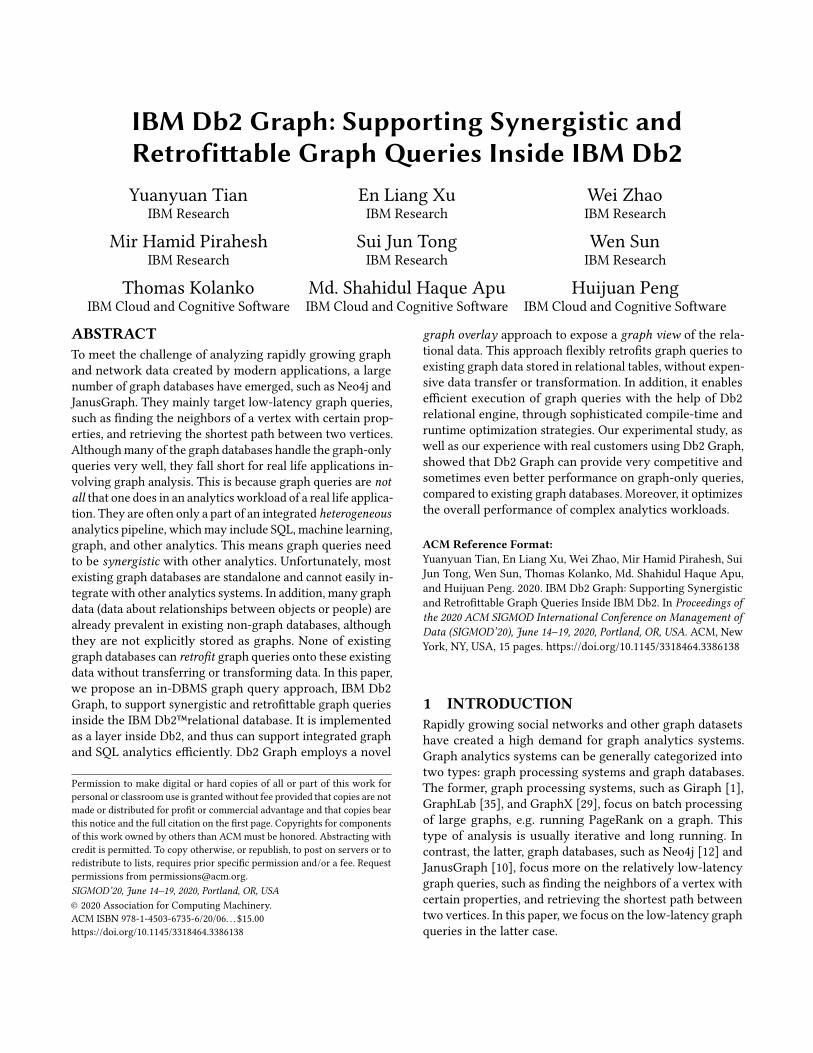
ABSTRACTTo meet the challenge of analyzing rapidly growing graphand network data created by modern applications, a largenumber of graph databases have emerged, such as Neo4j andJanusGraph. They mainly target low-latency graph queries,such as finding the neighbors of a vertex with certain prop-erties, and retrieving the shortest path between two vertices.Althoughmany of the graph databases handle the graph-onlyqueries very well, they fall short for real life applications in-volving graph analysis. This is because graph queries are notall that one does in an analytics workload of a real life applica-tion. They are often only a part of an integrated heterogeneousanalytics pipeline, whichmay include SQL, machine learning,graph, and other analytics. This means graph queries needto be synergistic with other analytics. Unfortunately, mostexisting graph databases are standalone and cannot easily in-tegrate with other analytics systems. In addition, many graphdata (data about relationships between objects or people) arealready prevalent in existing non-graph databases, althoughthey are not explicitly stored as graphs. None of existinggraph databases can retrofit graph queries onto these existingdata without transferring or transforming data. In this paper,we propose an in-DBMS graph query approach, IBM Db2Graph, to support synergistic and retrofittable graph queriesinside the IBM Db2™relational database. It is implementedas a layer inside Db2, and thus can support integrated graphand SQL analytics efficiently. Db2 Graph employs a novel

Permission to make digital or hard copies of all or part of this work forpersonal or classroom use is granted without fee provided that copies are notmade or distributed for profit or commercial advantage and that copies bearthis notice and the full citation on the first page. Copyrights for componentsof this work owned by others than ACMmust be honored. Abstracting withcredit is permitted. To copy otherwise, or republish, to post on servers or toredistribute to lists, requires prior specific permission and/or a fee. Requestpermissions from permissions@acm.org.SIGMOD’20, June 14–19, 2020, Portland, OR, USA© 2020 Association for Computing Machinery.ACM ISBN 978-1-4503-6735-6/20/06. . . $15.00https://doi.org/10.1145/3318464.3386138

graph overlay approach to expose a graph view of the rela-tional data. This approach flexibly retrofits graph queries toexisting graph data stored in relational tables, without expen-sive data transfer or transformation. In addition, it enablesefficient execution of graph queries with the help of Db2relational engine, through sophisticated compile-time andruntime optimization strategies. Our experimental study, aswell as our experience with real customers using Db2 Graph,showed that Db2 Graph can provide very competitive andsometimes even better performance on graph-only queries,compared to existing graph databases. Moreover, it optimizesthe overall performance of complex analytics workloads.

ACM Reference Format:Yuanyuan Tian, En Liang Xu, Wei Zhao, Mir Hamid Pirahesh, SuiJun Tong, Wen Sun, Thomas Kolanko, Md. Shahidul Haque Apu,and Huijuan Peng. 2020. IBM Db2 Graph: Supporting Synergisticand Retrofittable Graph Queries Inside IBM Db2. In Proceedings ofthe 2020 ACM SIGMOD International Conference on Management ofData (SIGMOD’20), June 14–19, 2020, Portland, OR, USA. ACM, NewYork, NY, USA, 15 pages. https://doi.org/10.1145/3318464.3386138

1 INTRODUCTIONRapidly growing social networks and other graph datasetshave created a high demand for graph analytics systems.Graph analytics systems can be generally categorized intotwo types: graph processing systems and graph databases.The former, graph processing systems, such as Giraph [1],GraphLab [35], and GraphX [29], focus on batch processingof large graphs, e.g. running PageRank on a graph. Thistype of analysis is usually iterative and long running. Incontrast, the latter, graph databases, such as Neo4j [12] andJanusGraph [10], focus more on the relatively low-latencygraph queries, such as finding the neighbors of a vertex withcertain properties, and retrieving the shortest path betweentwo vertices. In this paper, we focus on the low-latency graphqueries in the latter case.

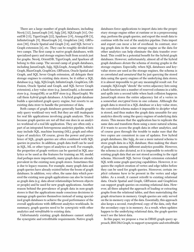
There are a large number of graph databases, includingNeo4j [12], JanusGraph [10], Sqlg [20], SQLGraph [41], Ori-entDB [15], TigerGraph [22], Sparksee [19], ArangoDB [3],InfiniteGraph [9], BlazeGraph [4], GraphGen [44], GRFu-sion [30], Oracle Spatial and Graph [14], and SQL Server’sGraph extension [6], etc. They can be roughly divided intotwo camps. The first camp is native graph databases, withspecialized query and storage engines built from scratch justfor graphs. Neo4j, OrientDB, TigerGraph, and Sparksee allbelong to this camp. The second camp of graph databases,including JanusGraph, Sqlg, SQLGraph, ArangoDB, Infinite-Graph, BlazeGraph, GraphGen, GRFusion, Oracle Spatial andGraph, and SQL Sever Graph extension, all delegate theirstorage engines to existing data stores, be it either a SQLdatabase (e.g. Sqlg, SQLGraph, InfiniteGraph, GraphGen, GR-Fusion, Oracle Spatial and Graph, and SQL Server Graphextension), a key-value store (e.g. JanusGraph), a documentstore (e.g. ArangoDB), or an RDF store (e.g. BlazeGraph). Wecall them hybrid graph databases. A hybrid graph databasebuilds a specialized graph query engine, but resorts to anexisting data store to handle the persistence of data.Both camps of graph databases generally handle graph-

only query workload very well. But they are still inadequatefor real life applications involving graph analysis. This isbecause graph queries are not all that one does in an analyt-ics workload of a real life application. They are often only apart of an integrated heterogeneous analytics pipeline, whichmay include SQL, machine learning (ML), graph and othertypes of analytics. Of course, given the power and preva-lence of SQL, graph queries are often combined with SQLqueries in practice. In addition, graph data itself can be usedin SQL, ML or other types of analytics as well. For example,the properties of graph vertices can be queried in SQL ana-lytics or be used as the features for training an ML model.And perhaps more importantly, many graph data are alreadyprevalent in the existing non-graph stores. Sometimes thisis due to legacy reasons. For example, many graph data andgraph queries have already existed before the boom of graphdatabases. In addition, very often, the same data which pow-ered the existing non-graph applications can also be treatedas graph data (e.g. data about relationships between objectsor people) and be used for new graph applications. Anotherreason behind the prevalence of graph data in non-graphstores is that the applications made conscious decisions tomanage graph queries themselves instead of using special-ized graph databases to achieve the good performance of theoverall applications with different analytics workloads. Insummary, graph queries need to be synergistic with otheranalytics and retrofittable to existing data.Unfortunately existing graph databases cannot satisfy

the synergistic and retrofittable requirements. Native graph

databases force applications to import data into the propri-etary storage engine either at runtime or in a preprocessingstep, perform the graph queries, and export the result data tocontinue with the rest of the analytics pipeline. Data importand export can incur a lot of overhead. In contrast, stor-ing graph data in the same storage engine as the data forother analytics can help eliminate the data transfer over-head. This could be a potential benefit for the hybrid graphdatabases. However, unfortunately, almost all of the hybridgraph databases dictate the schema of storing graphs in thestorage engines. Especially, when SQL databases and key-value stores are used as the storage engines, the schema isso convoluted and unnatural that by just querying the storeddata using the query engines of the underlying data stores,it is almost impossible to get any meaningful result out. Forexample, SQLGraph “shreds" the vertex adjacency lists usinga hash function into a number of reserved columns in a table,and spills into a second table when hash collision happens.JanusGraph stores the entire adjacency list of a vertex ina somewhat encrypted form in one column. Although thegraph data is stored in a SQL database or a key-value store,the convoluted schema makes it impossible to decipher whatis stored, and thus makes the graph data unusable for anyanalytics directly using the query engines of underlying datastores. This means that the application has to replicate thesame data and transform them using a more natural schema,if it wants to access the graph data in other analytics, andof course goes through the trouble to make sure that thetwo copies are consistent in case of updates. Few hybridgraph databases, like Sqlg, do use a more natural schema tostore graph data in a SQL database, thus making the shareof graph data among different analytics possible. However,the schema is also dictated, so it is impossible to retrofit toexisting graph data that are not stored according to the rigidschema. Microsoft SQL Server Graph extension extendedSQL with some graph querying capabilities. However, it re-quires the explicit creation of vertex and edge tables beforethey can be used for graph queries. Moreover, certain im-plicit columns have to be present in the vertex and edgetables. As a result, it cannot retrofit to existing relationaldata. Oracle Spatial and Graph, GRFusion and GraphGencan support graph queries on existing relational data. How-ever, all three adopted the approach of loading or extractinggraphs from the relational tables, and then materializing thegraph structures in memory. Graph queries are only servedon the in-memory copy of the data. Essentially, this approachalso keeps a second, transformed, copy of the data, only thatthe secondary copy is in memory. As a result, when updateshappen to the underlying relational data, the graph querieswon’t see the latest data.

In this paper, we propose a true in-DBMS graph query ap-proach, IBMDb2Graph, to support synergistic and retrofittable

Db2 Db2 Graph

GraphSQL

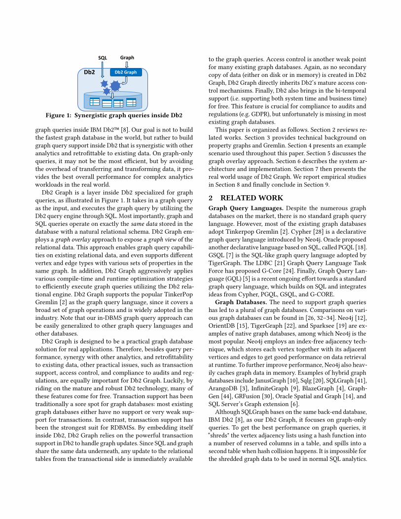
Figure 1: Synergistic graph queries inside Db2

graph queries inside IBM Db2™ [8]. Our goal is not to buildthe fastest graph database in the world, but rather to buildgraph query support inside Db2 that is synergistic with otheranalytics and retrofittable to existing data. On graph-onlyqueries, it may not be the most efficient, but by avoidingthe overhead of transferring and transforming data, it pro-vides the best overall performance for complex analyticsworkloads in the real world.

Db2 Graph is a layer inside Db2 specialized for graphqueries, as illustrated in Figure 1. It takes in a graph queryas the input, and executes the graph query by utilizing theDb2 query engine through SQL. Most importantly, graph andSQL queries operate on exactly the same data stored in thedatabase with a natural relational schema. Db2 Graph em-ploys a graph overlay approach to expose a graph view of therelational data. This approach enables graph query capabili-ties on existing relational data, and even supports differentvertex and edge types with various sets of properties in thesame graph. In addition, Db2 Graph aggressively appliesvarious compile-time and runtime optimization strategiesto efficiently execute graph queries utilizing the Db2 rela-tional engine. Db2 Graph supports the popular TinkerPopGremlin [2] as the graph query language, since it covers abroad set of graph operations and is widely adopted in theindustry. Note that our in-DBMS graph query approach canbe easily generalized to other graph query languages andother databases.Db2 Graph is designed to be a practical graph database

solution for real applications. Therefore, besides query per-formance, synergy with other analytics, and retrofittabilityto existing data, other practical issues, such as transactionsupport, access control, and compliance to audits and reg-ulations, are equally important for Db2 Graph. Luckily, byriding on the mature and robust Db2 technology, many ofthese features come for free. Transaction support has beentraditionally a sore spot for graph databases: most existinggraph databases either have no support or very weak sup-port for transactions. In contrast, transaction support hasbeen the strongest suit for RDBMSs. By embedding itselfinside Db2, Db2 Graph relies on the powerful transactionsupport in Db2 to handle graph updates. Since SQL and graphshare the same data underneath, any update to the relationaltables from the transactional side is immediately available

to the graph queries. Access control is another weak pointfor many existing graph databases. Again, as no secondarycopy of data (either on disk or in memory) is created in Db2Graph, Db2 Graph directly inherits Db2’s mature access con-trol mechanisms. Finally, Db2 also brings in the bi-temporalsupport (i.e. supporting both system time and business time)for free. This feature is crucial for compliance to audits andregulations (e.g. GDPR), but unfortunately is missing in mostexisting graph databases.This paper is organized as follows. Section 2 reviews re-

lated works. Section 3 provides technical background onproperty graphs and Gremlin. Section 4 presents an examplescenario used throughout this paper. Section 5 discusses thegraph overlay approach. Section 6 describes the system ar-chitecture and implementation. Section 7 then presents thereal world usage of Db2 Graph. We report empirical studiesin Section 8 and finally conclude in Section 9.

2 RELATEDWORKGraph Query Languages. Despite the numerous graphdatabases on the market, there is no standard graph querylanguage. However, most of the existing graph databasesadopt Tinkerpop Gremlin [2]. Cypher [28] is a declarativegraph query language introduced by Neo4j. Oracle proposedanother declarative language based on SQL, called PGQL [18].GSQL [7] is the SQL-like graph query language adopted byTigerGraph. The LDBC [21] Graph Query Language TaskForce has proposed G-Core [24]. Finally, Graph Query Lan-guage (GQL) [5] is a recent ongoing effort towards a standardgraph query language, which builds on SQL and integratesideas from Cypher, PGQL, GSQL, and G-CORE.

Graph Databases. The need to support graph querieshas led to a plural of graph databases. Comparisons on vari-ous graph databases can be found in [26, 32–34]. Neo4j [12],OrientDB [15], TigerGraph [22], and Sparksee [19] are ex-amples of native graph databases, among which Neo4j is themost popular. Neo4j employs an index-free adjacency tech-nique, which stores each vertex together with its adjacentvertices and edges to get good performance on data retrievalat runtime. To further improve performance, Neo4j also heav-ily caches graph data in memory. Examples of hybrid graphdatabases include JanusGraph [10], Sqlg [20], SQLGraph [41],ArangoDB [3], InfiniteGraph [9], BlazeGraph [4], Graph-Gen [44], GRFusion [30], Oracle Spatial and Graph [14], andSQL Server’s Graph extension [6].

Although SQLGraph bases on the same back-end database,IBM Db2 [8], as our Db2 Graph, it focuses on graph-onlyqueries. To get the best performance on graph queries, it“shreds" the vertex adjacency lists using a hash function intoa number of reserved columns in a table, and spills into asecond table when hash collision happens. It is impossible forthe shredded graph data to be used in normal SQL analytics.

Similar to Db2 Graph, Sqlg stores graph data in normalschema, but it dictates the schema. Therefore, it cannot retro-fit to existing relational data. At loading time, Sqlg analyzesall the data and decides on how to store the graph.

GraphGen extracts graphs from relational data via aDatalog-based DSL and stores a condensed in-memory representationof the extracted graphs. Graph queries and analytics are thencarried out on the in-memory representation. GRFusion [30]extends VoltDB [23] to define graph views on relational tables,and to materialize graph structures in memory for the graphqueries to execute on. Oracle Spatial and Graph [14] employsan access layer to ingest data from the Oracle databases orother sources into the Parallel Graph AnalytiX (PGX) [16],which is an in-memory graph analytic framework. All theabove three systems suffer from the same problem of query-ing staled data, in face of frequent updates.Microsoft SQL Server’s graph extension [6] also allows

some limited graph query capability inside the SQL Serverdatabase. However, it cannot retrofit to existing relationaltables. One has to create vertex table(s) and edge table(s) first,then populate data into these tables. Implicit columns areautomatically added to each vertex/edge table by the system,in order to uniquely identify each vertex/edge.Cytosm [40] is a middleware application that automati-

cally converts property graphs to the appropriate schemain a target backend storage (including relational databases)and translates Cypher queries to the target querying lan-guage. However, Cytosm doesn’t apply the sophisticated op-timization strategies that Db2 Graph employs during querycompilation and execution.

Graph Processing on RDBMSs. There are a number ofworks [27, 31, 45] that advocate using RDBMSs for batchgraph processing. However, they are not designed for low-latency graph queries, which is the focus of this paper.

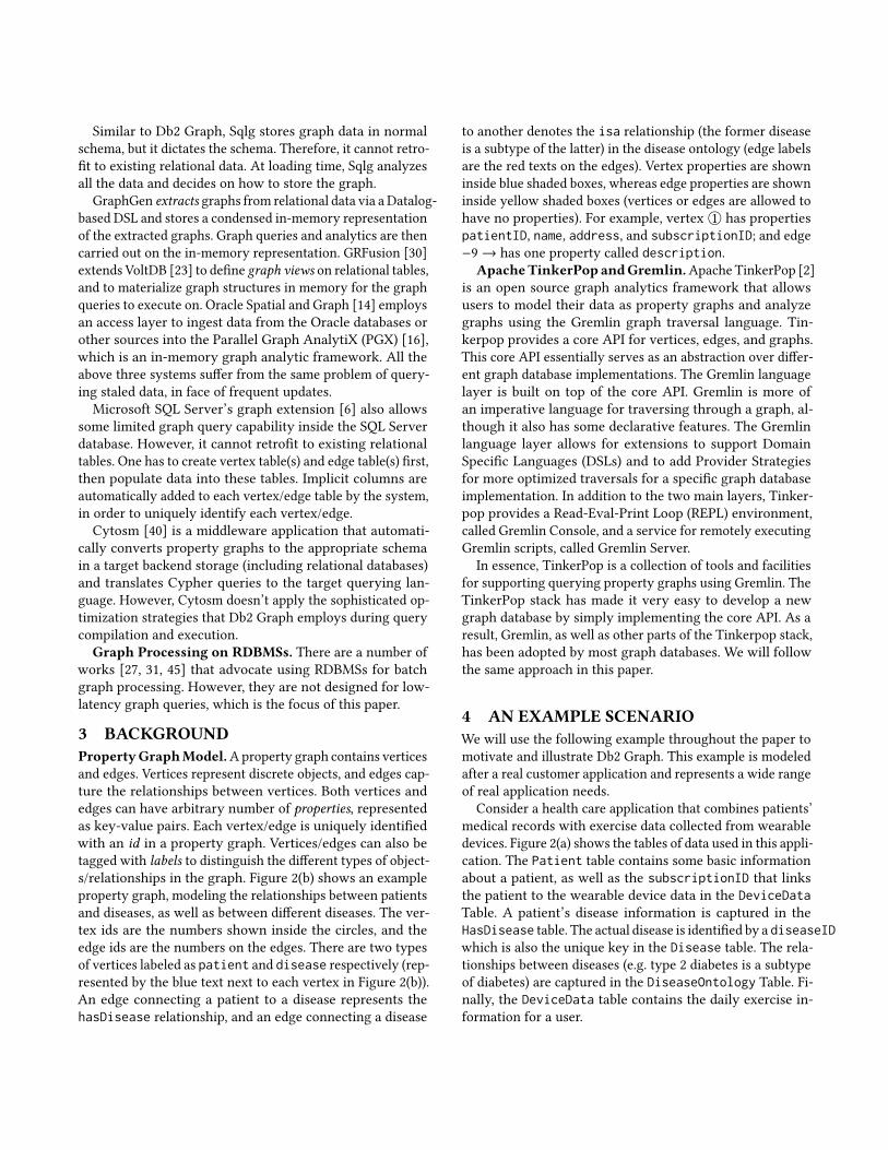
3 BACKGROUNDPropertyGraphModel.Aproperty graph contains verticesand edges. Vertices represent discrete objects, and edges cap-ture the relationships between vertices. Both vertices andedges can have arbitrary number of properties, representedas key-value pairs. Each vertex/edge is uniquely identifiedwith an id in a property graph. Vertices/edges can also betagged with labels to distinguish the different types of object-s/relationships in the graph. Figure 2(b) shows an exampleproperty graph, modeling the relationships between patientsand diseases, as well as between different diseases. The ver-tex ids are the numbers shown inside the circles, and theedge ids are the numbers on the edges. There are two typesof vertices labeled as patient and disease respectively (rep-resented by the blue text next to each vertex in Figure 2(b)).An edge connecting a patient to a disease represents thehasDisease relationship, and an edge connecting a disease

to another denotes the isa relationship (the former diseaseis a subtype of the latter) in the disease ontology (edge labelsare the red texts on the edges). Vertex properties are showninside blue shaded boxes, whereas edge properties are showninside yellow shaded boxes (vertices or edges are allowed tohave no properties). For example, vertex 1○ has propertiespatientID, name, address, and subscriptionID; and edge−9 → has one property called description.ApacheTinkerPop andGremlin.Apache TinkerPop [2]

is an open source graph analytics framework that allowsusers to model their data as property graphs and analyzegraphs using the Gremlin graph traversal language. Tin-kerpop provides a core API for vertices, edges, and graphs.This core API essentially serves as an abstraction over differ-ent graph database implementations. The Gremlin languagelayer is built on top of the core API. Gremlin is more ofan imperative language for traversing through a graph, al-though it also has some declarative features. The Gremlinlanguage layer allows for extensions to support DomainSpecific Languages (DSLs) and to add Provider Strategiesfor more optimized traversals for a specific graph databaseimplementation. In addition to the two main layers, Tinker-pop provides a Read-Eval-Print Loop (REPL) environment,called Gremlin Console, and a service for remotely executingGremlin scripts, called Gremlin Server.

In essence, TinkerPop is a collection of tools and facilitiesfor supporting querying property graphs using Gremlin. TheTinkerPop stack has made it very easy to develop a newgraph database by simply implementing the core API. As aresult, Gremlin, as well as other parts of the Tinkerpop stack,has been adopted by most graph databases. We will followthe same approach in this paper.

4 AN EXAMPLE SCENARIOWe will use the following example throughout the paper tomotivate and illustrate Db2 Graph. This example is modeledafter a real customer application and represents a wide rangeof real application needs.

Consider a health care application that combines patients’medical records with exercise data collected from wearabledevices. Figure 2(a) shows the tables of data used in this appli-cation. The Patient table contains some basic informationabout a patient, as well as the subscriptionID that linksthe patient to the wearable device data in the DeviceDataTable. A patient’s disease information is captured in theHasDisease table. The actual disease is identified by a diseaseIDwhich is also the unique key in the Disease table. The rela-tionships between diseases (e.g. type 2 diabetes is a subtypeof diabetes) are captured in the DiseaseOntology Table. Fi-nally, the DeviceData table contains the daily exercise in-formation for a user.

diseaseID conceptCode conceptName

64572326 44054006 “Type 2 diabetes”

… …

subscriptionID date steps execiseMinutes activeEnergy

115 11/15/2018 9039 25 208

… … … …

patientID diseaseID description

1 64572326 …

… … …

patientID name address subscriptionID

1 Alice … 115

… …

Disease Table

DeviceData Table

HasDisease TablePatient Table

sourceID targetID type

64572326 73211009 “isa”

… …

DiseaseOntology Table

(a) Example tables

12

5

3 4

6

78

patientID = 1name = “Alice”address = …subscriptionID = …

patientID = 2name = “Charlie”address = …subscriptionID: …

patientID = 2name = “Bob”address = …subscriptionID: …

9 hasDisease

10

description = …

description = …

diseaseID = 64572326conceptCode = …conceptName = “Type 2 diabetes”

diseaseID = 64572476conceptCode = …conceptName = “Type 1 diabetes”

diseaseID = 64572345conceptCode = …conceptName = “Diabetes”

diseaseID = 64582824conceptCode = …conceptName = “Disorder of glucose metabolism ”

diseaseID = 64562633conceptCode = …conceptName = “Hypoglycemic Syndrome”

isa

isa

isa

isa

hasDiseasedescription = …

hasDisease description = …

13

16

12

11

14

15

patient

patient

patient

disease

disease

disease

disease

hasDisease

disease

(b) The property graph modeled on some example tables

Figure 2: An example scenario

The patients’ medical records and the disease ontologydata have always been stored in the relational database tosupport the existing applications of the customer. However,the customer also wants to support new applications thatcombine these data with wearable device data. In addition,they also wish to view the patient-to-disease and the disease-to-disease relationships (the 4 tables in the dashed-line box ofFigure 2(a)) in the context of a graph as shown in Figure 2(b)and query the graph. Moreover, the new applications will re-quire integrating graph queries with SQL analytics together.Db2 Graph provides three interfaces for users to con-

duct graph queries: a command line interface called Gremlinconsole, a simple Db2 table function for submitting graphqueries inside SQL, and programming APIs in a number ofhost languages including Java, Scala, Python and Groovy.As a result, there are different ways Db2 Graph can supportsynergistic SQL and graph queries together in one appli-cation. At the developing stage, users can have a SQL con-sole and a Gremlin console opened side by side to querythe same underlying data either as relational tables or as aproperty graph. The demo in [42] showed such an ad hocinsurance claim analysis using Db2 Graph (video availableat https://www.youtube.com/watch?v=C5vmcYKEN-U).

Db2 Graph introduces a simple polymorphic table func-tion [17] in Db2, called graphQuery, to submit graph queriesinside SQL and bring the results back as a table1. For example,the following SQL statement finds patients that have similardiseases as those of a particular patient (with patientID=1),and compares their daily exercise patterns.SELECT patientID, AVG(steps), AVG(execiseMinutes)FROM DeviceData AS D,TABLE (graphQuery(‘gremlin’, ‘similar_diseases = g.V().hasLabel(\‘patient\’).has(\‘patientID\’, \‘1\’).out(\‘hasDisease\’).repeat(out(\‘isa\’).dedup().store(\‘x\’)).times(2).repeat(in(\‘isa\’).dedup().store(\‘x\’)).times(2).cap(\‘x\’).next();g.V(similar_diseases).in(\‘hasDisease\’).dedup().values(\‘patientID\’, \‘subscriptionID\’)’))AS P (patientID long, subscriptionID long)

WHERE D.subscriptionID = P.subscriptionIDGROUP BY patientID

In this query, finding the patients with similar diseasesis done inside a graph query (highlighted in blue): it firsttraverses from the patient vertex to the connecting diseasevertices, then traverses the disease ontology 2-hops up and2-hops down, collecting all the diseases encountered alongthe way as similar diseases, finally finds all the patients thathave any of these diseases and returns their patientIDsand subscriptionIDs. Afterwards, SQL joins the resultingtable with the DeviceData table, and aggregates the averagesteps and execiseMinutes per patient.

At production stage, applications often use the JDBC APIalong with the programming API of Db2 Graph to mix SQLand graph queries in one workload. This approach is themost flexible and powerful in performing synergistic graphand SQL queries together in one application.

The example scenario described in this section is the per-fect embodiment of the synergy between SQL and graphqueries. Each does what it is good at, and together accom-plish the task synergistically. Graph queries excels at navi-gating through complex relationships, whereas SQL is goodat the heavy-lifting group-by and aggregation.Using Db2 Graph, there is no need to have a separate

system to handle graph queries, and even no need to replicatethe four tables in a different format just for graph queries.Everything can be done in the same Db2 with no change tothe existing tables. As a result, the graph data is always upto date with the latest information from the transactionalsystem. For example, when patient information changes,the graph queries see these changes immediately. Moreover,the temporal support in Db2 allows all of our graphs to betemporal as well. For example, one can view a graph "as of"different time snapshots.

1Note that the graphQuery function only supports Gremlin graph querieswith return results that can be converted into a collection of rows.

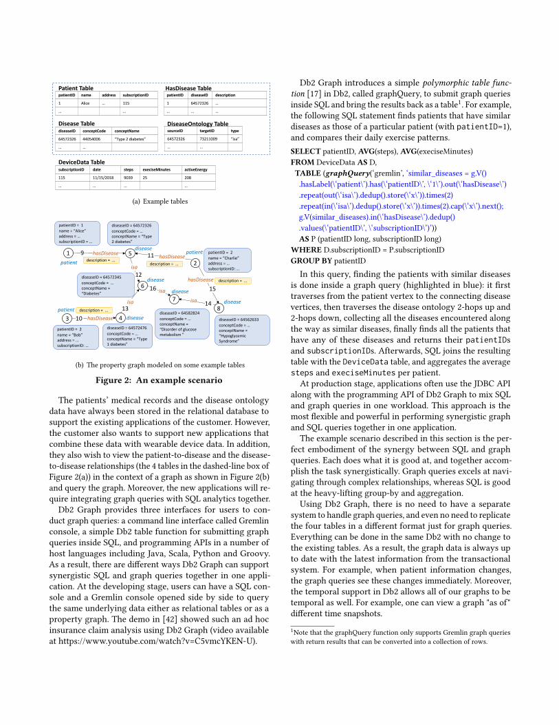
5 OVERLAYING GRAPHS ON TABLESIn this section, we describe the graph overlay approach inDb2 Graph. Graph databases always present a single prop-erty graph with a vertex set and an edge set for users toquery. Of course, the single graph doesn’t have to be fullyconnected, and there can be different types of vertices andedges. In Db2 Graph, we essentially map each vertex/edgein the vertex/edge set to a single row in the database. Over-laying a single property graph onto a set of relational tablesreally boils down to mapping the vertex set and the edge setof the graph to the relational tables.

For the vertex set, the mapping needs to specify: 1) whattable(s) store the vertex information, 2) what table column(s)are mapped to the required id field, 3) what is the label foreach vertex (defined from a table column or a constant), and4) what columns capture the vertex properties, if any. Simi-larly, for the edge set, the mapping needs to specify: 1) whattable(s) store the edge information, 2) what table columnsare mapped to the required id, src_v (source vertex id), anddst_v (destination vertex id) fields, 3) what is the label foreach edge (defined from a table column or a constant), and 4)what columns correspond to the edge properties, if any. Thisgraph overlay mapping is achieved by an overlay configura-tion file in Db2 Graph. Note that the mapping is not restrictedto tables only, it can be also on created views of tables. Be-low, we show an example overlay configuration file in JSONformat for mapping a property graph like in Figure 2(b) tothe 4 tables in the dashed-line box of Figure 2(a).

1 "v_tables": [2 {3 "table_name": "Patient",4 "prefixed_id": true ,5 "id": "'patient ':: patientID",6 "fix_label": true ,7 "label": "'patient '",8 "properties": ["patientID", "name", "address", "

subscriptionID"]9 },10 {11 "table_name": "Disease",12 "id": "diseaseID",13 "fix_label": true ,14 "label": "'disease '",15 "properties": ["diseaseID", "conceptCode", "

conceptName"]16 }],17 "e_tables": [18 {19 "table_name": "DiseaseOntology",20 "src_v_table": "Disease",21 "src_v": "sourceID",22 "dst_v_table": "Disease",23 "dst_v": "targetID",24 "prefixed_edge_id": true ,25 "id": "'ontology ':: sourceID :: targetID",26 "label": "type"27 },28 {29 "table_name": "HasDisease",30 "src_v_table": "Patient",31 "src_v": "'patient ':: patientID",32 "dst_v_table": "Disease",

33 "dst_v": "diseaseID",34 "implicit_edge_id": true ,35 "fix_label": true ,36 "label": "'hasDisease '"37 }]

The configuration file defines a set of vertex tables (v_tables,Line 1-16) for representing the vertex set of the propertygraph, as well as a set of edge tables (e_tables, Line 17-37) for representing the edge set of the property graph. Inthis example, Patient and Disease are the vertex tables,and DiseaseOntology and HasDisease are the edge tables.Then for each such vertex/edge table, it specifies how todefine the required fields of a vertex/edge, as well as theproperties. For a vertex, the required fields are id and label;for an edge, the required fields are id, label, src_v (sourcevertex id), and dst_v (destination vertex id).

In the property graph model, the id field is a requirementfor each vertex and it has to be unique across the entiregraph. The id field can be defined by one or more columnsthat uniquely identify a vertex, like column diseaseID inLine 12. However, when there are multiple relational tablesmapping to the vertex set of a property graph, the unique keyof a table may not always uniquely identify the associatedvertex in the whole vertex set (across tables). As a result, weneed to prefix the unique key with a unique table identifier todefine the id field of a vertex. The unique table identifier canbe the table name or some other unique constant value. Thisis the reason why Line 4 sets prefixed_id to true, and Line5 defines id as "‘patient’::patientID". Here ‘patient’is a string constant, which serves as a unique table identifierof the Patient table. If prefixed_id is not set, it is false bydefault. As will be discussed in Section 6.3, prefixed ids canlead to more optimized performance at runtime.

The label field is also required in the property graphmodel.It can be mapped either to a column of the table, e.g. columntype in Line 26, or to a constant, e.g. ‘patient’ in Line7. In common practice, different types of vertices or edgesare typically stored in separate tables, which implies that allvertices or edges in a single table share the same label value.This means it is not necessary, and sometimes not possible, touse a column (in most cases, there is no such column) in therelational table to define the label field. For this reason, weintroduce a feature to specify that all vertices or edges froma table have the same label and set that label to a constantstring value. Lines 6 and 7 show such an example for thePatient table. As we will discuss in Section 6.3, this featureprovides an optimization opportunity to narrow down theset of tables to query from at runtime.Besides id and label fields, each edge table also needs to

describe how the source and destination vertex ids, src_vand dst_v respectively, are defined. If all the source/desti-nation vertices of an edge table come from one vertex table,

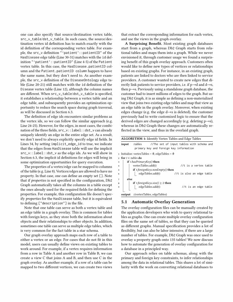
one can also specify that source/destination vertex table,src_v_table/dst_v_table. In such cases, the source/des-tination vertex id definition has to match exactly with theid definition of the corresponding vertex table. For exam-ple, the src_v definition "‘patient’::patientID" of theHasDisease edge table (Line 30-31) matches with the id def-inition "‘patient’::patientID" (Line 4-5) of the Patientvertex table. In this case, the HasDisease.patientID col-umn and the Patient.patientID column happen to havethe same name, but they don’t need to. As another exam-ple, the src_v definition of the DiseaseOntology edge ta-ble (Line 20-21) still matches with the id definition of theDisease vertex table (Line 12), although the column namesare different. When src_v_table/dst_v_table is specified,it establishes a relationship between a vertex table and anedge table, and subsequently provides an optimization op-portunity to reduce the search space during graph traversal,as will be discussed in Section 6.3.

The definition of edge ids encounters similar problems asthe vertex ids, so we can follow the similar approach (e.g.Line 24-25). However, for the edges, in most cases, the combi-nation of the three fields, src_v::label::dst_v can alreadyuniquely identify an edge in the entire edge set. As a result,we don’t need to always explicitly specify edge id fields. InLines 34, by setting implicit_edge_id to true, we indicatethat the edges from HasDisease table will use the implicitsrc_v::label::dst_v as the edge ids. As we will show inSection 6.3, the implicit id definitions for edges will bring insome optimization opportunities for query execution.

The properties of a vertex/edge can be mapped to columnsof the table (e.g. Line 8). Vertices/edges are allowed to have noproperty. In that case, one can define an empty set []. Notethat if properties is not specified in the configuration, Db2Graph automatically takes all the columns in a table exceptthe ones already used for the required fields for defining theproperties. For example, this configuration file doesn’t spec-ify properties for the HasDisease table, but it is equivalentto defining ["description"] in the file.Note that one table can serve as both a vertex table and

an edge table in a graph overlay. This is common for tableswith foreign keys, as they store both the information aboutobjects and their relationships to other objects. In addition,sometimes one table can serve as multiple edge tables, whichis very common for the fact table in a star schema.Our graph overlay approach maps each row of a table to

either a vertex or an edge. For cases that do not fit in thismodel, users can usually define views on existing tables towork around. For example, if a vertex requires informationfrom a row in Table A and another row in Table B, we cancreate a view C that joins A and B, and then use C in thegraph overlay. As another example, if a row of a table can bemapped to two different vertices, we can create two views

that extract the corresponding information for each vertex,and use the views in the graph overlay.

A Surprising Benefit. Most existing graph databasesstart from a graph, whereas Db2 Graph starts from rela-tional tables and maps them into a graph. While we neverenvisioned it, through customer usage we found a surpris-ing benefit of this graph overlay approach. Customers oftenwould like to define new types of vertices or relationshipsbased on existing graphs. For instance, in an existing graph,patients are linked to doctors who are then linked to serviceproviders. A customer wanted to create new edges that di-rectly link patients to service providers, i.e. if p→d and d→s,then p→s. Previously using a standalone graph database, thecustomer had to insert millions of edges to the graph. But us-ing Db2 Graph, it is as simple as defining a non-materializedview that joins two existing edge tables and map that view asan edge table in the graph overlay. Moreover, when existingedges change (e.g. the edge d→s is deleted), the customerpreviously had to write customized logic to ensure that thederived edges are changed accordingly (e.g. deleting p→s),whereas in Db2 Graph these changes are automatically re-flected in the view, and thus in the overlaid graph.

ALGORITHM 1: Identify Vertex Tables and Edge Tablesinput : tables //The set of input tables with schema and

primary key and foreign key information

1 Initialize: vertexTables = ∅, edgeTables = ∅

2 for t ∈ tables do3 if t.hasPrimaryKey() then4 vertexTables.add(t) //t is a vertex table

5 if t.foreignKeys.nonEmpty() then6 edgeTables.add(t) //t is also an edge table

7 else8 if t.foreignKeys.size() ≥ 2 then9 edgeTables.add(t) //t is an edge table

output : (vertexTables, edgeTables)

5.1 Automatic Overlay GenerationThe overlay configuration files can be manually created bythe application developers who wish to query relational ta-bles as graphs. One can create multiple overlay configurationfiles on the same set of tables, so that they can be queriedas different graphs. Manual specification provides a lot offlexibility, but can also be labor intensive, if there are a largenumber of tables. For example, Db2 Graph was once used tooverlay a property graph onto 135 tables! We now discusshow to automate the generation of overlay configuration fora database in a principled way.Our approach relies on table schemas, along with the

primary and foreign key constraints, to infer relationshipsamong the data in relational tables. This shares a lot of simi-larity with the work on converting relational databases to

ALGORITHM 2: Generate Overlay Configurationinput :vertexTables, edgeTables

1 Initialize: vertexTableConfs = ∅, edgeTableConfs = ∅

2 for t ∈ vertexTables do3 vtc = newVertexTableConf()4 vtc.idField = combine(t.uniqueID, t.primaryKey)5 vtc.hasFixedLabel = true6 vtc.fixedLabel = t.tableName7 vtc.propertyFields = t.columns - t.primaryKey8 vertexTableConfs.add(vtc)

9 for t ∈ edgeTables do10 if t.hasPrimaryKey() then11 for fk ∈ t.foreignKeys do12 etc = newEdgeTableConf()13 etc.hasImplicitEdgeID = true14 etc.srcvTable = t.tableName15 etc.srcvField = combine(t.uniqueID, t.primaryKey)16 etc.dstvTable = fk.refTable.tableName17 etc.dstvField = combine(fk.refTable.uniqueID, fk)18 etc.hasFixedLabel = true19 etc.fixedLabel = concat(t.tableName, fk.refTable.tableName)20 etc.propertyFields = t.columns - t.primaryKey - fk21 edgeTableConfs.add(etc)

22 else23 for fk1, fk2 ∈ t.foreignKeys and fk1,fk2 do24 etc = newEdgeTableConf()25 etc.hasImplicitEdgeID = true26 etc.srcvTable = fk1.refTable.tableName27 etc.srcvField = combine(fk1.refTable.uniqueID, fk1)28 etc.dstvTable = fk2.refTable.tableName29 etc.dstvField = combine(fk2.refTable.uniqueID, fk2)30 etc.hasFixedLabel = true31 etc.fixedLabel = concat(fk1.refTable.tableName, t.tableName,

fk2.refTable.tableName)32 etc.propertyFields = t.columns - fk1 - fk233 edgeTableConfs.add(etc)

output : (vertexTableConfs, edgeTableConfs)

graph databases [25, 36–38, 43], since the data conversionalso uses schema and functional dependencies to convert re-lational data to graphs. But the major difference between thetwo is that data conversion creates a completely new copyof the original data, whereas graph overlay merely createsa virtual graph view on top of the original data. As a result,the graph overlay generation needs to come up with a graphschema that more faithfully captures the semantics of therelational data, whereas the data conversion approaches canhave more freedom. For example, the approach in [25] makesevery attribute (column) of a table as a vertex in the graph.

Db2 Graph provides a toolkit, called AutoOverlay, for au-tomatically generating a graph overlay. A user can specifywhich database he/she wants to generate the overlay con-figuration for. If only a subset of tables in a database are

of interest, the user can also explicitly list these tables. Au-toOverlay automatically generates the overlay configurationin the following steps:

Step 1: AutoOverlay first queries Db2 catalog to get all themetadata information for each table such as table schema,and primary key/foreign key constraints.

Step 2: Then, it iterates through all tables to find out thevertex tables and edge tables as shown in Algorithm 1. Notethat a table can serve as both a vertex table and an edge table.Any table with a primary key will be served as a vertex table.If a table has a primary key and one or more foreign keys(e.g. a fact table in a star schema), it will also be used as oneor more edge tables, one for each foreign key. If a table hask (k ≥ 2) foreign keys but no primary key (many-to-manyrelationships), then it will be used as

(k2)edge tables, one for

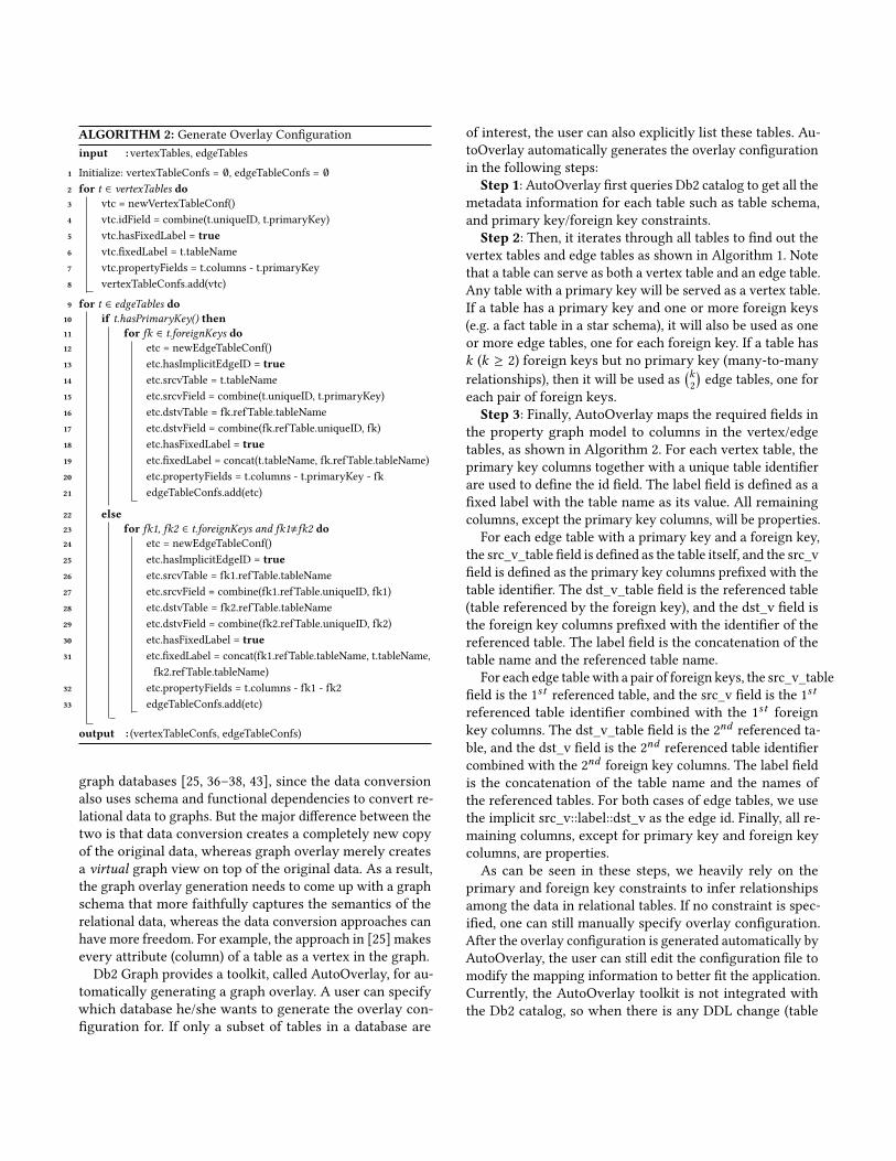
each pair of foreign keys.Step 3: Finally, AutoOverlay maps the required fields in

the property graph model to columns in the vertex/edgetables, as shown in Algorithm 2. For each vertex table, theprimary key columns together with a unique table identifierare used to define the id field. The label field is defined as afixed label with the table name as its value. All remainingcolumns, except the primary key columns, will be properties.

For each edge table with a primary key and a foreign key,the src_v_table field is defined as the table itself, and the src_vfield is defined as the primary key columns prefixed with thetable identifier. The dst_v_table field is the referenced table(table referenced by the foreign key), and the dst_v field isthe foreign key columns prefixed with the identifier of thereferenced table. The label field is the concatenation of thetable name and the referenced table name.

For each edge tablewith a pair of foreign keys, the src_v_tablefield is the 1st referenced table, and the src_v field is the 1streferenced table identifier combined with the 1st foreignkey columns. The dst_v_table field is the 2nd referenced ta-ble, and the dst_v field is the 2nd referenced table identifiercombined with the 2nd foreign key columns. The label fieldis the concatenation of the table name and the names ofthe referenced tables. For both cases of edge tables, we usethe implicit src_v::label::dst_v as the edge id. Finally, all re-maining columns, except for primary key and foreign keycolumns, are properties.As can be seen in these steps, we heavily rely on the

primary and foreign key constraints to infer relationshipsamong the data in relational tables. If no constraint is spec-ified, one can still manually specify overlay configuration.After the overlay configuration is generated automatically byAutoOverlay, the user can still edit the configuration file tomodify the mapping information to better fit the application.Currently, the AutoOverlay toolkit is not integrated withthe Db2 catalog, so when there is any DDL change (table

Topology Graph Structure

SQL Dialect

TraversalStrategy

Db2 Query Engine

SQL

Db2

Gra

phGremlin

load overlay info call API

generate

SQL

apply

strategies

access

overlay info

TinkerPop GraphStep HasStep VertexSteplogical plan

Db2Graph.vertices()

HasStep. filter()

Db2Vertex.edges()

physical planDb2Graph.open()

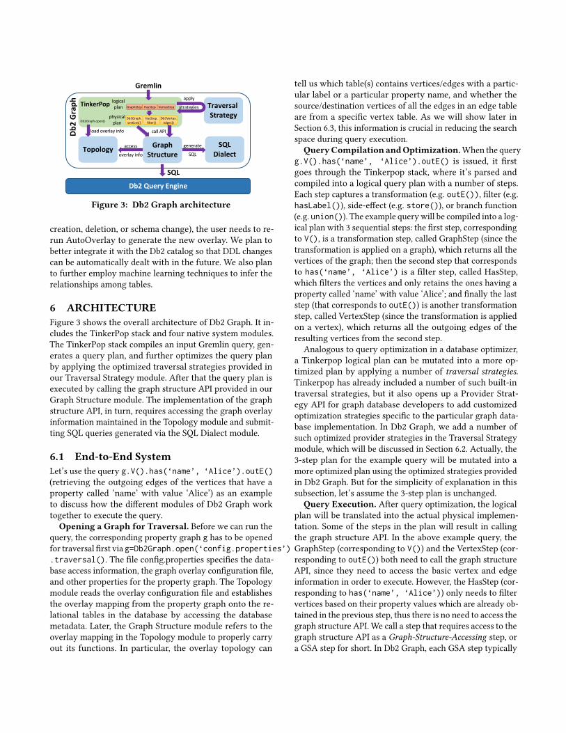
Figure 3: Db2 Graph architecture

creation, deletion, or schema change), the user needs to re-run AutoOverlay to generate the new overlay. We plan tobetter integrate it with the Db2 catalog so that DDL changescan be automatically dealt with in the future. We also planto further employ machine learning techniques to infer therelationships among tables.

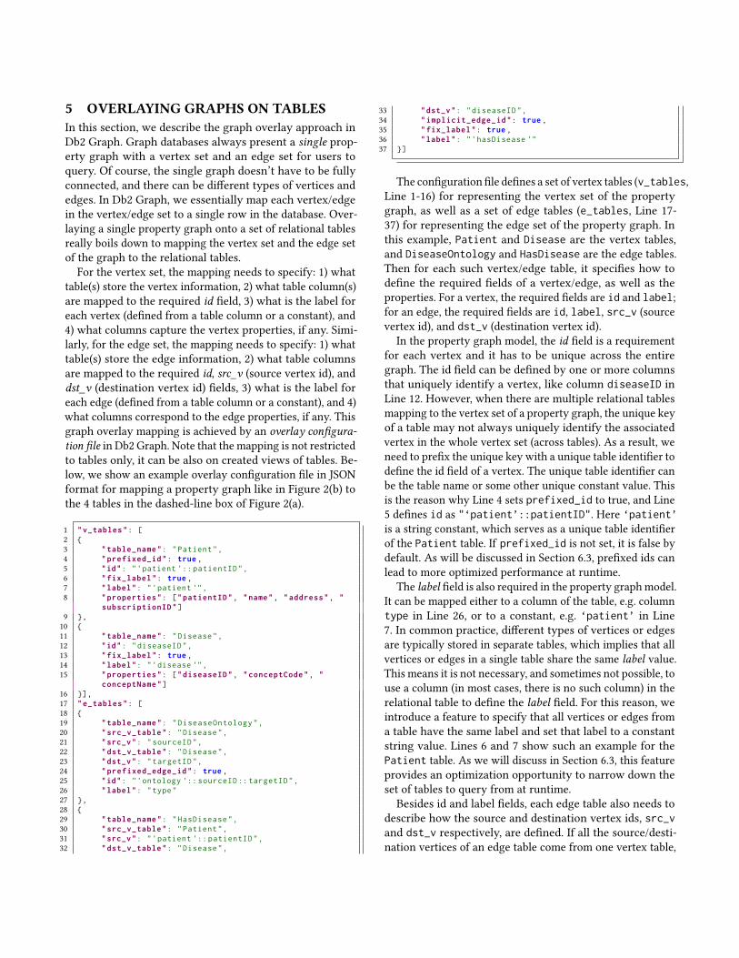
6 ARCHITECTUREFigure 3 shows the overall architecture of Db2 Graph. It in-cludes the TinkerPop stack and four native system modules.The TinkerPop stack compiles an input Gremlin query, gen-erates a query plan, and further optimizes the query planby applying the optimized traversal strategies provided inour Traversal Strategy module. After that the query plan isexecuted by calling the graph structure API provided in ourGraph Structure module. The implementation of the graphstructure API, in turn, requires accessing the graph overlayinformation maintained in the Topology module and submit-ting SQL queries generated via the SQL Dialect module.

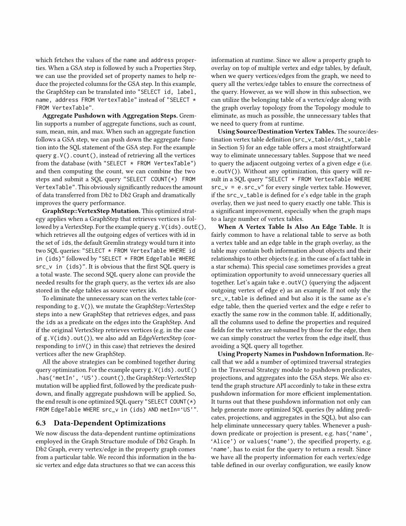
6.1 End-to-End SystemLet’s use the query g.V().has(‘name’, ‘Alice’).outE()(retrieving the outgoing edges of the vertices that have aproperty called ‘name’ with value ‘Alice’) as an exampleto discuss how the different modules of Db2 Graph worktogether to execute the query.

Opening a Graph for Traversal. Before we can run thequery, the corresponding property graph g has to be openedfor traversal first via g=Db2Graph.open(‘config.properties’).traversal(). The file config.properties specifies the data-base access information, the graph overlay configuration file,and other properties for the property graph. The Topologymodule reads the overlay configuration file and establishesthe overlay mapping from the property graph onto the re-lational tables in the database by accessing the databasemetadata. Later, the Graph Structure module refers to theoverlay mapping in the Topology module to properly carryout its functions. In particular, the overlay topology can

tell us which table(s) contains vertices/edges with a partic-ular label or a particular property name, and whether thesource/destination vertices of all the edges in an edge tableare from a specific vertex table. As we will show later inSection 6.3, this information is crucial in reducing the searchspace during query execution.

QueryCompilation andOptimization.When the queryg.V().has(‘name’, ‘Alice’).outE() is issued, it firstgoes through the Tinkerpop stack, where it’s parsed andcompiled into a logical query plan with a number of steps.Each step captures a transformation (e.g. outE()), filter (e.g.hasLabel()), side-effect (e.g. store()), or branch function(e.g. union()). The example querywill be compiled into a log-ical plan with 3 sequential steps: the first step, correspondingto V(), is a transformation step, called GraphStep (since thetransformation is applied on a graph), which returns all thevertices of the graph; then the second step that correspondsto has(‘name’, ‘Alice’) is a filter step, called HasStep,which filters the vertices and only retains the ones having aproperty called ‘name’ with value ‘Alice’; and finally the laststep (that corresponds to outE()) is another transformationstep, called VertexStep (since the transformation is appliedon a vertex), which returns all the outgoing edges of theresulting vertices from the second step.

Analogous to query optimization in a database optimizer,a Tinkerpop logical plan can be mutated into a more op-timized plan by applying a number of traversal strategies.Tinkerpop has already included a number of such built-intraversal strategies, but it also opens up a Provider Strat-egy API for graph database developers to add customizedoptimization strategies specific to the particular graph data-base implementation. In Db2 Graph, we add a number ofsuch optimized provider strategies in the Traversal Strategymodule, which will be discussed in Section 6.2. Actually, the3-step plan for the example query will be mutated into amore optimized plan using the optimized strategies providedin Db2 Graph. But for the simplicity of explanation in thissubsection, let’s assume the 3-step plan is unchanged.

Query Execution. After query optimization, the logicalplan will be translated into the actual physical implemen-tation. Some of the steps in the plan will result in callingthe graph structure API. In the above example query, theGraphStep (corresponding to V()) and the VertexStep (cor-responding to outE()) both need to call the graph structureAPI, since they need to access the basic vertex and edgeinformation in order to execute. However, the HasStep (cor-responding to has(‘name’, ‘Alice’)) only needs to filtervertices based on their property values which are already ob-tained in the previous step, thus there is no need to access thegraph structure API. We call a step that requires access to thegraph structure API as a Graph-Structure-Accessing step, ora GSA step for short. In Db2 Graph, each GSA step typically

results in one or more SQL queries to Db2. We can affect theexecution of these steps through our implementation of thecorresponding graph structure API.The Graph Structure module contains our implementa-

tion of the Tinkerpop graph structure API. The basic graphstructure API includes Graph, Vertex, Edge, VertexProperty,and Property, as well as graph operations on them, such asgetting vertices/edges by ids and getting the adjacent ver-tices/edges of a vertex/edge. We also extend the basic API tocarry out more sophisticated functionalities (e.g. predicate,projection, and aggregate pushdown) in response to the op-timized query plans resulted from applying the optimizedstrategies from the Traversal Strategy module, as will bediscussed in Section 6.3. The Graph Structure module refersto the overlay mapping in the Topology module to decide onhow to implement graph operations. The implementationof the graph structure API affects the execution of all theGSA steps in Db2 Graph, so we strive to optimize as muchas possible. In Section 6.3, we will highlight how we applythe data-dependent optimizations at runtime by utilizing thegraph overlay topology. Finally, the Graph Structure mod-ule utilizes the SQL Dialect module to translate the graphoperations into SQL queries.

The SQL Dialect module deals with everything related toDb2. It generates all the SQL queries needed for implement-ing graph operations. This module also keep tracks of theseSQL queries and finds out frequent query patterns. For ex-ample, if the name column is frequently used (above a pre-setthreshold) in the predicates for querying the Patient table,the SQL Dialect module will consider it as a frequent querypattern. It then creates a set of pre-compiled SQL templatesfor these frequent patterns and issues the correspondingprepare statements in Db2 to avoid the SQL compilationoverhead at runtime. Based on these SQL templates, it alsosuggests indexes (e.g. an index on the name column of thePatient table) that would speed up the execution of thetranslated SQL queries. This module can also provide hintsto the Db2 index advisor, which can look at the entire work-load and advise indexes.Let’s take the 3-step logical plan for the example query,

and illustrate how it is executed. Note again that the ac-tual execution of this query is much more optimized in Db2Graph. But, we stick with this naive version of the executionfor the simplicity of explanation. Only the GraphStep andthe VertexStep in this plan are GSA steps, thus only thesetwo actually call our graph structure API implementation.Each API function implementation needs to decide 1) whatrelational tables to query from, and 2) for each table, whatSQL query to submit. The GraphStep, corresponding to V(),retrieves all vertices from the graph. So, only vertex tablesneed to be queried. But there is no extra information to helpus narrow down a subset of the vertex tables. As a result,

for every vertex table, we need to submit a SQL query like"SELECT * FROM VertexTable". The second HasStep, corre-sponding to has(‘name’,‘Alice’), is executed inside Db2Graph (no SQL query is needed). And finally the VertexStep,corresponding to outE(), needs to query every edge tableand submit a SQL query like "SELECT * FROM EdgeTablewhere src in (id1, id2, ...)", where id1, id2 and soon are the ids of the vertices from step 2.

Obviously, the above execution plan is very inefficient: thefirst step returns all the vertices in the graph even thoughthe second step would filter out most of the vertices. Inthe following two subsections, we describe the optimizationtechniques employed in Db2 Graph to address the ineffi-ciency. These optimization techniques aim at 1) eliminatingthe unnecessary tables to query from, and 2) generatingmoreoptimized SQL queries to reduce the query latency and thereturned results for each necessary table. The optimizationtechniques can be grouped into two categories. The first cat-egory is all about the optimized traversal strategies in theTraversal Strategy module applied during query optimiza-tion. These techniques are data-independent, i.e. they don’tneed to know anything about the underlying relational dataor how they are mapped to the property graph. In compari-son, the techniques in the second category are all applied atthe runtime execution in the Graph Structure module. Andthey are data-dependent, i.e. they need to access the graphoverlay mapping information in the Topology module.

6.2 Optimized Traversal StrategiesWe first discuss the data-independent, optimized, traversalstrategies in the Traversal Strategy module applied duringquery optimization. The traversal strategies mutate a queryplan whenever a pattern is matched, eventually generatingmore optimized SQL queries. For all of these optimized strate-gies, we start from a GSA step, since it results in SQL calls.

Predicate Pushdown with Filter Steps. When a GSAstep is followed by a sequence of filter steps, we can fold thesefilter steps as extra predicates into the GSA step. Consider thefirst two steps of the previous example query g.V().has(‘name’,‘Alice’). Now, the HasStep can be folded into the Graph-Step. And the new GraphStep with the extra predicate can betranslated into one SQL query "SELECT * FROM VertexTableWHERE name = ‘Alice’". We basically push down all thefilter steps into the “where" clause of the SQL statement forthe GSA step (the filter steps are all removed in the optimizedplan), which results in a significant reduction of the SQL run-time and the results returned from the database. This is, insome sense, very similar to query push down in the settingof federated databases [39].

Projection Pushdown with Properties Steps. Graphtraversals often fetch some particular vertex or edge prop-erties, for example g.V().values(‘name’, ‘address’),

which fetches the values of the name and address proper-ties. When a GSA step is followed by such a Properties Step,we can use the provided set of property names to help re-duce the projected columns for the GSA step. In this example,the GraphStep can be translated into "SELECT id, label,name, address FROM VertexTable" instead of "SELECT *FROM VertexTable".Aggregate Pushdown with Aggregation Steps. Grem-

lin supports a number of aggregate functions, such as count,sum, mean, min, and max. When such an aggregate functionfollows a GSA step, we can push down the aggregate func-tion into the SQL statement of the GSA step. For the examplequery g.V().count(), instead of retrieving all the verticesfrom the database (with "SELECT * FROM VertexTable")and then computing the count, we can combine the twosteps and submit a SQL query "SELECT COUNT(*) FROMVertexTable". This obviously significantly reduces the amountof data transferred from Db2 to Db2 Graph and dramaticallyimproves the query performance.

GraphStep::VertexStepMutation. This optimized strat-egy applies when a GraphStep that retrieves vertices is fol-lowed by aVertexStep. For the example query g.V(ids).outE(),which retrieves all the outgoing edges of vertices with id inthe set of ids, the default Gremlin strategy would turn it intotwo SQL queries: "SELECT * FROM VertexTable WHERE idin (ids)" followed by "SELECT * FROM EdgeTable WHEREsrc_v in (ids)". It is obvious that the first SQL query isa total waste. The second SQL query alone can provide theneeded results for the graph query, as the vertex ids are alsostored in the edge tables as source vertex ids.

To eliminate the unnecessary scan on the vertex table (cor-responding to g.V()), we mutate the GraphStep::VertexStepsteps into a new GraphStep that retrieves edges, and passthe ids as a predicate on the edges into the GraphStep. Andif the original VertexStep retrieves vertices (e.g. in the caseof g.V(ids).out()), we also add an EdgeVertexStep (cor-responding to inV() in this case) that retrieves the desiredvertices after the new GraphStep.

All the above strategies can be combined together duringquery optimization. For the example query g.V(ids).outE().has(‘metIn’, ‘US’).count(), the GraphStep::VertexStepmutation will be applied first, followed by the predicate push-down, and finally aggregate pushdown will be applied. So,the end result is one optimized SQL query "SELECT COUNT(*)FROM EdgeTable WHERE src_v in (ids) AND metIn=‘US’".

6.3 Data-Dependent OptimizationsWe now discuss the data-dependent runtime optimizationsemployed in the Graph Structure module of Db2 Graph. InDb2 Graph, every vertex/edge in the property graph comesfrom a particular table. We record this information in the ba-sic vertex and edge data structures so that we can access this

information at runtime. Since we allow a property graph tooverlay on top of multiple vertex and edge tables, by default,when we query vertices/edges from the graph, we need toquery all the vertex/edge tables to ensure the correctness ofthe query. However, as we will show in this subsection, wecan utilize the belonging table of a vertex/edge along withthe graph overlay topology from the Topology module toeliminate, as much as possible, the unnecessary tables thatwe need to query from at runtime.

Using Source/DestinationVertexTables.The source/des-tination vertex table definition (src_v_table/dst_v_tablein Section 5) for an edge table offers a most straightforwardway to eliminate unnecessary tables. Suppose that we needto query the adjacent outgoing vertex of a given edge e (i.e.e.outV()). Without any optimization, this query will re-sult in a SQL query "SELECT * FROM VertexTable WHEREsrc_v = e.src_v" for every single vertex table. However,if the src_v_table is defined for e’s edge table in the graphoverlay, then we just need to query exactly one table. This isa significant improvement, especially when the graph mapsto a large number of vertex tables.

When A Vertex Table Is Also An Edge Table. It isfairly common to have a relational table to serve as botha vertex table and an edge table in the graph overlay, as thetable may contain both information about objects and theirrelationships to other objects (e.g. in the case of a fact table ina star schema). This special case sometimes provides a greatoptimization opportunity to avoid unnecessary queries alltogether. Let’s again take e.outV() (querying the adjacentoutgoing vertex of edge e) as an example. If not only thesrc_v_table is defined and but also it is the same as e’sedge table, then the queried vertex and the edge e refer toexactly the same row in the common table. If, additionally,all the columns used to define the properties and requiredfields for the vertex are subsumed by those for the edge, thenwe can simply construct the vertex from the edge itself, thusavoiding a SQL query all together.

UsingPropertyNames inPushdown Information.Re-call that we add a number of optimized traversal strategiesin the Traversal Strategy module to pushdown predicates,projections, and aggregates into the GSA steps. We also ex-tend the graph structure API accordinly to take in these extrapushdown information for more efficient implementation.It turns out that these pushdown information not only canhelp generate more optimized SQL queries (by adding predi-cates, projections, and aggregates in the SQL), but also canhelp eliminate unnecessary query tables. Whenever a push-down predicate or projection is present, e.g. has(‘name’,‘Alice’) or values(‘name’), the specified property, e.g.‘name’, has to exist for the query to return a result. Sincewe have all the property information for each vertex/edgetable defined in our overlay configuration, we easily know

whether the specified property exists or not in a vertex/edgetable. Then, only the tables having the required propertyneed to be queried.

Using Label Values. Label is a very special property ina property graph, thus a very common operation in Gremlinis to retrieve vertices/edges by label(s), e.g.g.V().hasLabel(‘patient’) and v.outE(‘hasDisease’).Naively, this would result in querying through all the ver-tex/edge tables with a predicate on the given label(s). But,our graph overlay configuration allows a vertex/edge tableto have a fixed label (i.e. fixed_label is true) for all thevertices/edges in it. When this happens, we can use the spec-ified label(s) to narrow down a subset of vertex/edge tables toquery from. More specifically, any table that has a fixed labelbut not matched with the query label(s) can be eliminatedfrom the query. Note that the implementation still has tosearch all the tables without fixed labels to make sure it isnot missing any results. This optimization provides a hugeperformance improvement.

Using Prefixed Id Values. Another very basic operationin the graph structure API is looking up vertices/edges byids. When a given id is a prefixed id (unique key prefixedwith a unique table identifier), e.g. ‘patient’::1, we canuse the unique table identifier to pin down the exact table tosearch from (in this example, the Patient table), instead ofblindly querying through all the tables. In addition, when theid field is the concatenation of multiple table columns (e.g.‘TableName’::c1::c2), Db2 Graph extracts the individualcolumn values from an id value and forms conjunctive predi-cates (e.g. c1=c1_value and c2=c2_value) in SQL queries.

Using Implicit Edge Id Values. For edge ids definedwith the implicit src_v::label::dst_v combination, when fixedlabels are specified for edge tables, we can also utilize thelabel encoded in the id field to narrow down the tables tosearch from for looking up an edge by its id, similar to howwe eliminate tables using label values. Similar to the prefixedid values, Db2 Graph also breaks apart the implicit edge idvalues to form conjunctive predicates in SQL queries.

7 REAL WORLD USAGEDb2 Graph has been used in a number of real customer en-gagements. In finance, an example application is mule frauddetection, where graph queries are used to detect how a setof fraudsters are connected to a set of beneficiaries througha sequence of mule accounts. The dataset for this applica-tion is bank transaction data, which are updated frequentlythrough the bank’s operational functions and also used byexisting SQL analytical applications. The timeliness of thefraud detection requires the graph queries to access the latesttransaction data. As a result, importing all the transactiondata to a standalone graph database would be expensive andhard to satisfy the timeliness requirement.

In health care, Db2 Graph has been used for patient casestudy on a dataset that contains patient EMR records, hos-pital discharges, and health insurance information. This ap-plication views patients, hospital discharges, diagnoses, labresults, medical procedures, drugs, and insurance enrollmentinformation etc. all as vertices of a graph. The queries tra-verse through the graph to find out how a patient is treatedin an inpatient service (e.g. what tests have been done, whatprocedures have been performed, what diagnoses have beenmade, and what drugs have been given), as well as how thecosts are covered by insurance. These are path queries start-ing from a single vertex. There are already a large numberof existing applications reading and writing this dataset, andthe graph queries need to work on the latest data. In addition,the demo in [42] showed another detailed scenario for healthinsurance claim analysis using Db2 Graph. In this applica-tion, SQL and graph queries need to work synergistically,hence using a standalone graph database would not be ideal.

In law enforcement, Db2 Graph has been used to query apolice department dataset that contains information aboutpersons (suspects, victims, or witnesses), organizations (legit-imate organizations or gangs), arrests, warrants, complaints,vehicles, locations, emails, and phones. The application viewsall these entities as vertices and conducts case studies, such asfinding the phone numbers and addresses of the suspects inan arrest, and figuring out the criminal organizations that allsuspects of an arrest belong to. Again the workload consistsof path queries starting from a single vertex. The dataset isupdated in real time, thus using a standalone graph databasewould be hard to keep data up-to-date for graph queries.

So far, the largest real graph that Db2 Graph has workedon, contains about 4 billion vertices and 6 billion edges withroughly half a terabyte of data. The graph workload consistsof Gremlin queries that traverse from some vertices, satisfy-ing certain conditions, up to 4 hops away, with optional pred-icates on the traversal paths. The observed average queryresponse time using Db2 Graph is sub 100 milliseconds.

8 EVALUATIONIn the following, we report experimental results of Db2Graph on a synthetic benchmark. Recall that we focus on thescenarios where graph data already exist in the relationaldatabase, and the design goal of Db2 Graph is not to be thefastest in graph-only queries. Nevertheless, we still comparethe graph query performance of Db2 Graph against two state-of-the-art graph-only databases: GDB-X, a commercial high-performance native graph database (the name is anonymizeddue to the sensitivity of reporting its performance numbers),and JanusGraph [10], a popular open-source graph database(with Berkeley DB [13] as the backend store).

We used the Linkbench [11] graph benchmark for perfor-mance evaluation. Here, we only focus on the query only

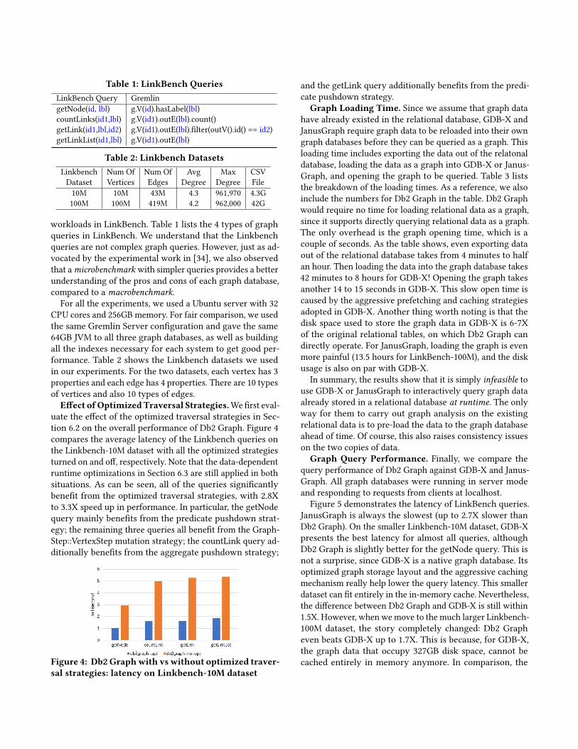
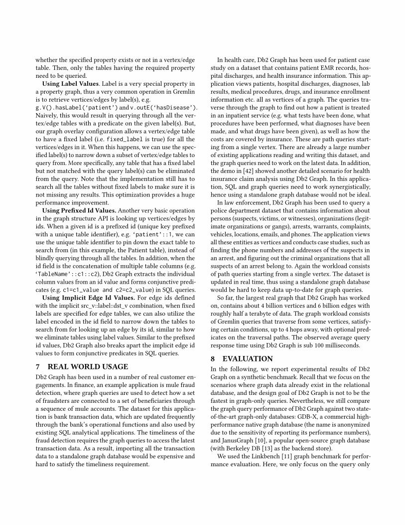
Table 1: LinkBench QueriesLinkBench Query GremlingetNode(id, lbl) g.V(id).hasLabel(lbl)countLinks(id1,lbl) g.V(id1).outE(lbl).count()getLink(id1,lbl,id2) g.V(id1).outE(lbl).filter(outV().id() == id2)getLinkList(id1,lbl) g.V(id1).outE(lbl)

Table 2: Linkbench DatasetsLinkbench Num Of Num Of Avg Max CSVDataset Vertices Edges Degree Degree File10M 10M 43M 4.3 961,970 4.3G100M 100M 419M 4.2 962,000 42G

workloads in LinkBench. Table 1 lists the 4 types of graphqueries in LinkBench. We understand that the Linkbenchqueries are not complex graph queries. However, just as ad-vocated by the experimental work in [34], we also observedthat amicrobenchmark with simpler queries provides a betterunderstanding of the pros and cons of each graph database,compared to a macrobenchmark.

For all the experiments, we used a Ubuntu server with 32CPU cores and 256GB memory. For fair comparison, we usedthe same Gremlin Server configuration and gave the same64GB JVM to all three graph databases, as well as buildingall the indexes necessary for each system to get good per-formance. Table 2 shows the Linkbench datasets we usedin our experiments. For the two datasets, each vertex has 3properties and each edge has 4 properties. There are 10 typesof vertices and also 10 types of edges.

Effect ofOptimizedTraversal Strategies.Wefirst eval-uate the effect of the optimized traversal strategies in Sec-tion 6.2 on the overall performance of Db2 Graph. Figure 4compares the average latency of the Linkbench queries onthe Linkbench-10M dataset with all the optimized strategiesturned on and off, respectively. Note that the data-dependentruntime optimizations in Section 6.3 are still applied in bothsituations. As can be seen, all of the queries significantlybenefit from the optimized traversal strategies, with 2.8Xto 3.3X speed up in performance. In particular, the getNodequery mainly benefits from the predicate pushdown strat-egy; the remaining three queries all benefit from the Graph-Step::VertexStep mutation strategy; the countLink query ad-ditionally benefits from the aggregate pushdown strategy;

Figure 4: Db2 Graphwith vs without optimized traver-sal strategies: latency on Linkbench-10M dataset

and the getLink query additionally benefits from the predi-cate pushdown strategy.

Graph Loading Time. Since we assume that graph datahave already existed in the relational database, GDB-X andJanusGraph require graph data to be reloaded into their owngraph databases before they can be queried as a graph. Thisloading time includes exporting the data out of the relatonaldatabase, loading the data as a graph into GDB-X or Janus-Graph, and opening the graph to be queried. Table 3 liststhe breakdown of the loading times. As a reference, we alsoinclude the numbers for Db2 Graph in the table. Db2 Graphwould require no time for loading relational data as a graph,since it supports directly querying relational data as a graph.The only overhead is the graph opening time, which is acouple of seconds. As the table shows, even exporting dataout of the relational database takes from 4 minutes to halfan hour. Then loading the data into the graph database takes42 minutes to 8 hours for GDB-X! Opening the graph takesanother 14 to 15 seconds in GDB-X. This slow open time iscaused by the aggressive prefetching and caching strategiesadopted in GDB-X. Another thing worth noting is that thedisk space used to store the graph data in GDB-X is 6-7Xof the original relational tables, on which Db2 Graph candirectly operate. For JanusGraph, loading the graph is evenmore painful (13.5 hours for LinkBench-100M), and the diskusage is also on par with GDB-X.

In summary, the results show that it is simply infeasible touse GDB-X or JanusGraph to interactively query graph dataalready stored in a relational database at runtime. The onlyway for them to carry out graph analysis on the existingrelational data is to pre-load the data to the graph databaseahead of time. Of course, this also raises consistency issueson the two copies of data.

Graph Query Performance. Finally, we compare thequery performance of Db2 Graph against GDB-X and Janus-Graph. All graph databases were running in server modeand responding to requests from clients at localhost.Figure 5 demonstrates the latency of LinkBench queries.

JanusGraph is always the slowest (up to 2.7X slower thanDb2 Graph). On the smaller Linkbench-10M dataset, GDB-Xpresents the best latency for almost all queries, althoughDb2 Graph is slightly better for the getNode query. This isnot a surprise, since GDB-X is a native graph database. Itsoptimized graph storage layout and the aggressive cachingmechanism really help lower the query latency. This smallerdataset can fit entirely in the in-memory cache. Nevertheless,the difference between Db2 Graph and GDB-X is still within1.5X. However, when wemove to the much larger Linkbench-100M dataset, the story completely changed: Db2 Grapheven beats GDB-X up to 1.7X. This is because, for GDB-X,the graph data that occupy 327GB disk space, cannot becached entirely in memory anymore. In comparison, the

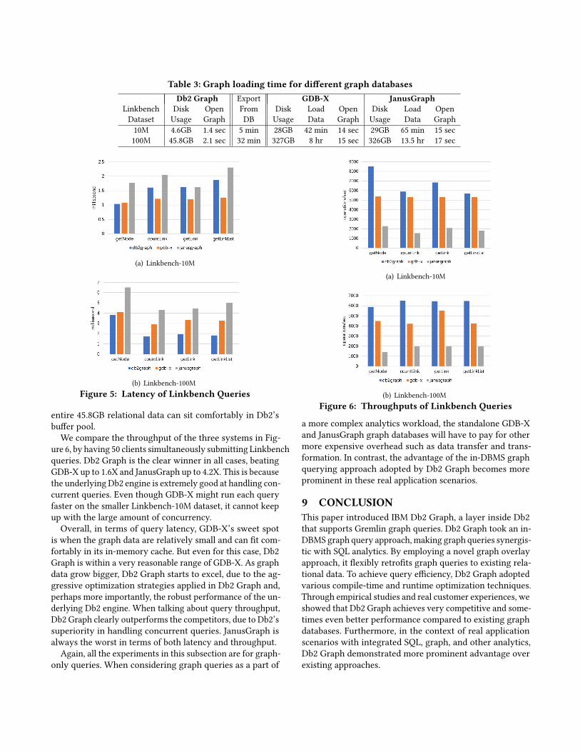
Table 3: Graph loading time for different graph databasesDb2 Graph Export GDB-X JanusGraph

Linkbench Disk Open From Disk Load Open Disk Load OpenDataset Usage Graph DB Usage Data Graph Usage Data Graph10M 4.6GB 1.4 sec 5 min 28GB 42 min 14 sec 29GB 65 min 15 sec100M 45.8GB 2.1 sec 32 min 327GB 8 hr 15 sec 326GB 13.5 hr 17 sec

(a) Linkbench-10M

(b) Linkbench-100MFigure 5: Latency of Linkbench Queries

entire 45.8GB relational data can sit comfortably in Db2’sbuffer pool.We compare the throughput of the three systems in Fig-

ure 6, by having 50 clients simultaneously submitting Linkbenchqueries. Db2 Graph is the clear winner in all cases, beatingGDB-X up to 1.6X and JanusGraph up to 4.2X. This is becausethe underlying Db2 engine is extremely good at handling con-current queries. Even though GDB-X might run each queryfaster on the smaller Linkbench-10M dataset, it cannot keepup with the large amount of concurrency.Overall, in terms of query latency, GDB-X’s sweet spot

is when the graph data are relatively small and can fit com-fortably in its in-memory cache. But even for this case, Db2Graph is within a very reasonable range of GDB-X. As graphdata grow bigger, Db2 Graph starts to excel, due to the ag-gressive optimization strategies applied in Db2 Graph and,perhaps more importantly, the robust performance of the un-derlying Db2 engine. When talking about query throughput,Db2 Graph clearly outperforms the competitors, due to Db2’ssuperiority in handling concurrent queries. JanusGraph isalways the worst in terms of both latency and throughput.

Again, all the experiments in this subsection are for graph-only queries. When considering graph queries as a part of

(a) Linkbench-10M

(b) Linkbench-100MFigure 6: Throughputs of Linkbench Queries

a more complex analytics workload, the standalone GDB-Xand JanusGraph graph databases will have to pay for othermore expensive overhead such as data transfer and trans-formation. In contrast, the advantage of the in-DBMS graphquerying approach adopted by Db2 Graph becomes moreprominent in these real application scenarios.

9 CONCLUSIONThis paper introduced IBM Db2 Graph, a layer inside Db2that supports Gremlin graph queries. Db2 Graph took an in-DBMS graph query approach, making graph queries synergis-tic with SQL analytics. By employing a novel graph overlayapproach, it flexibly retrofits graph queries to existing rela-tional data. To achieve query efficiency, Db2 Graph adoptedvarious compile-time and runtime optimization techniques.Through empirical studies and real customer experiences, weshowed that Db2 Graph achieves very competitive and some-times even better performance compared to existing graphdatabases. Furthermore, in the context of real applicationscenarios with integrated SQL, graph, and other analytics,Db2 Graph demonstrated more prominent advantage overexisting approaches.

REFERENCES[1] Apache Giraph. http://giraph.apache.org.[2] Apache TinkerPop. http://http://tinkerpop.apache.org.[3] ArangoDB. https://www.arangodb.com.[4] BlazeGraph. https://www.blazegraph.com.[5] GQL. https://www.gqlstandards.org.[6] Graph processing with SQL Server and Azure SQL Database.

https://docs.microsoft.com/en-us/sql/relational-databases/graphs/sql-graph-overview?view=sql-server-2017.

[7] GSQL. https://www.tigergraph.com/gsql.[8] IBM Db2. https://www.ibm.com/analytics/us/en/db2.[9] InfiniteGraph. https://www.objectivity.com/products/infinitegraph.[10] JanusGraph. http://janusgraph.org.[11] LinkBench: A database benchmark for the social graph.

https://www.facebook.com/notes/facebook-engineering/linkbench-a-database-benchmark-for-the-social-graph/10151391496443920.

[12] Neo4j. https://neo4j.com.[13] Oracle Berkeley DB. http://www.oracle.com/technetwork/database/

database-technologies/berkeleydb/overview/index.html.[14] Oracle Spatial and Graph. https://www.oracle.com/database/

technologies/spatialandgraph.html.[15] OrientDB. https://orientdb.com.[16] Parallel Graph AnalytiX (PGX). https://www.oracle.com/technetwork/

oracle-labs/parallel-graph-analytix/overview/index.html.[17] Polymorphic table functions in SQL. https://standards.iso.org/ittf/

PubliclyAvailableStandards/c069776_ISO_IEC_TR_19075-7_2017.zip.[18] PQGL. http://pgql-lang.org.[19] Sparksee. http://www.sparsity-technologies.com.[20] Sqlg. http://www.sqlg.org.[21] The graph and RDF benchmark reference. http://ldbcouncil.org.[22] TigerGraph. https://www.tigergraph.com.[23] VoltDB. https://www.voltdb.com.[24] R. Angles, M. Arenas, P. Barcelo, P. Boncz, G. Fletcher, C. Gutierrez,

T. Lindaaker, M. Paradies, S. Plantikow, J. Sequeda, O. van Rest, andH. Voigt. G-core: A core for future graph query languages. In SIGMOD’18, pages 1421–1432, 2018.

[25] R. De Virgilio, A. Maccioni, and R. Torlone. Converting relational tograph databases. In GRADES ’13, pages 1:1–1:6, 2013.

[26] D. Dominguez-Sal, P. Urbón-Bayes, A. Giménez-Vañó, S. Gómez-Villamor, N. Martínez-Bazán, and J. L. Larriba-Pey. Survey of graphdatabase performance on the hpc scalable graph analysis benchmark.In WAIM’10, pages 37–48, 2010.

[27] J. Fan, A. G. S. Raj, and J. M. Patel. The case against specialized graphanalytics engines. In CIDR ’15, 2015.

[28] N. Francis, A. Green, P. Guagliardo, L. Libkin, T. Lindaaker, V. Marsault,S. Plantikow, M. Rydberg, P. Selmer, and A. Taylor. Cypher: An evolv-ing query language for property graphs. In SIGMOD ’18, pages 1433–1445, 2018.

[29] J. E. Gonzalez, R. S. Xin, A. Dave, D. Crankshaw, M. J. Franklin, andI. Stoica. Graphx: Graph processing in a distributed dataflow frame-work. In OSDI’14, pages 599–613, 2014.

[30] M. S. Hassan, T. Kuznetsova, H. C. Jeong, W. G. Aref, and M. Sadoghi.Grfusion: Graphs as first-class citizens in main-memory relationaldatabase systems. In SIGMOD ’18, pages 1789–1792, 2018.

[31] A. Jindal, S. Madden, M. Castellanos, and M. Hsu. Graph analyticsusing vertica relational database. In IEEE Big Data ’15, pages 1191–1200,2015.

[32] S. Jouili and V. Vansteenberghe. An empirical comparison of graphdatabases. In SOCIALCOM ’13, pages 708–715, 2013.

[33] V. Kolomičenko, M. Svoboda, and I. H. Mlýnková. Experimental com-parison of graph databases. In IIWAS ’13, pages 115:115–115:124, 2013.

[34] M. Lissandrini, M. Brugnara, and Y. Velegrakis. Beyond macrobench-marks: Microbenchmark-based graph database evaluation. PVLDB,12(4):390–403, 2018.

[35] Y. Low, D. Bickson, J. Gonzalez, C. Guestrin, A. Kyrola, and J. M. Heller-stein. Distributed GraphLab: a framework for machine learning anddata mining in the cloud. PVLDB, 5(8):716–727, 2012.

[36] Y. A. Megid, N. El-Tazi, and A. Fahmy. Using functional dependenciesin conversion of relational databases to graph databases. In Databaseand Expert Systems Applications, pages 350–357, 2018.

[37] O. Orel, S. Zakosek, and M. Baranovic. Property oriented relational-to-graph database conversion. Automatika, 57(3):836–845, 2016.

[38] S. Pradhan, S. Chakravarthy, and A. Telang. Modeling relational dataas graphs for mining. In COMAD ’09, 2009.

[39] A. P. Sheth and J. A. Larson. Federated database systems for man-aging distributed, heterogeneous, and autonomous databases. ACMComputing Surveys, 22(3):183–236, 1990.

[40] B. A. Steer, A. Alnaimi, M. A. B. F. G. Lotz, F. Cuadrado, L. M. Vaquero,and J. Varvenne. Cytosm: Declarative property graph queries withoutdata migration. In Proceedings of the Fifth International Workshop onGraph Data-management Experiences & Systems, GRADES’17, pages4:1–4:6, 2017.

[41] W. Sun, A. Fokoue, K. Srinivas, A. Kementsietsidis, G. Hu, and G. Xie.Sqlgraph: An efficient relational-based property graph store. In SIG-MOD ’15, pages 1887–1901, 2015.

[42] Y. Tian, S. J. Tong, M. H. Pirahesh, W. Sun, E. L. Xu, and W. Zhao.Synergistic graph and SQL analytics Inside IBM Db2. PVLDB, 12(12),2019.

[43] D. W. Wardani and J. Kiing. Semantic mapping relational to graphmodel. In IC3INA ’14, pages 160–165, 2014.

[44] K. Xirogiannopoulos and A. Deshpande. Extracting and analyzinghidden graphs from relational databases. In SIGMOD ’17, pages 897–912, 2017.

[45] K. Zhao and J. X. Yu. All-in-one: Graph processing in rdbmss revisited.In SIGMOD ’17, pages 1165–1180, 2017.