1

Different approaches of modelling reaction lags: How do Chilean

manufacturing exports react to movements of the real exchange rate?

by

Felicitas Nowak-Lehmann D.

Ibero-Amerika Institut fuer Wirtschaftsforschung, University of Goettingen

Gosslerstr. 1B, 37073 Goettingen, Germany

e-mail: fnowak@gwdg.de

Abstract

This study examines the relationship between export supply and the real

exchange rate using annual Chilean data for the period 1960-96. The hypotheses

to be tested are first, that the real exchange rate does matter for the supply of

exports - contrary to studies relying on quarterly data - and second, that the

impact of a real depreciation only ceases to be positive and significant after about

2-3 years. Four different distributed lag models were considered as potentially

adequate and useful to depict the impact of the real exchange rate over time.

Even though all four models assumed different underlying lag structures, they all

point to the importance of maintaining a competitive real exchange rate over time.

The transfer function model is particularly well-suited in shaping any lag structure

in that it is not presumptive in form.

JEL classification codes: C22, F31, F41

Key words: distributed lag models; impact of the real exchange rate on

manufactured exports

2

1. Introduction

Chile, an early reformer in Latin America, undertook many changes in its

exchange rate regime and its exchange rate policy in the period between 1960

and 20021. Resulting changes in real exchange rates and their lagged impact on

exports are relevant for two reasons: First, the Chilean economy is not only good

in exporting but also very dependent on exports. Second, the approach of

modelling lags might also be interesting when other countries and/or other

economic issues are investigated.

The most important changes in Chilean economic policy occurred in 1973/74

under the military regime of Pinochet (1973-89) when policy-making underwent an

orientation towards neoliberal and monetarist thinking. This fully market-oriented

economic policy was continued under Aylwin (1990-95) and Frei (1995-2000) to

the surprise of many neoliberal economists and political observers who had

expected a return to interventionist policy-making under the Christian Democrats.

Since then, this policy has even been taken up in general terms by President

Lagos who belongs to the socialist party.

It is worthwhile to mention that the exchange rate continued to play an important

part in Chilean economic policy making both under Pinochet and the Christian

Democrats, Aylwin and Frei. After having removed the multiple exchange rate

system of the interventionist days and after having unsuccessfully applied an

orthodox anti-inflation policy during 1973 to 1977, the monetarist economic team

started to use the exchange rate to tame inflation by pursuing an active crawling

peg in 1978/79, causing the rate of devaluation to fall behind the rate of inflation.

3

The result of real appreciation of the Chilean peso was reinforced and the rate of

inflation finally curbed, by fixing the Chilean peso to the US-$ in 1979. This policy

found its justification in theories of ‘Global Monetarism’ that considered and

suggested fixing the exchange rate as a way to bring down the rate of price

increases of an inflation-prone country to the lower world rate of inflation via a

shrinking of the supply of money. However, in 1982 the nominal anchor system

had to be given up due to unsustainable current account deficits. The currency

had to be devalued and in 1984 a more flexible crawling peg regime vis-à-vis the

US-$ with an exchange rate band of +/- 5% was introduced. Since 1991 the

Chilean peso was fixed to a currency basket consisting of the US-$, the German

mark and the yen. The exchange rate band was then extended to +/- 10%. Due to

high capital inflows, however, the Chilean peso had to be revalued in nominal

terms whenever the lower exchange rate band was reached. Furthermore, real

appreciations resulted because the Chilean rate of inflation, though low for Latin

American standards, continued to exceed the respective rates of the U.S.A,

Germany and Japan. This being the case, Chilean exporters complained louder in

the last few years. Given this constant appreciation pressure on the real

exchange rate, a flexible exchange rate regime was introduced on September 2,

1999. In 2001, all remaining controls on capital transactions were eliminated (IMF,

2000 and 2002).

The question now is whether an appreciated real exchange rate does harm to

exports, and if so, to what extent. Another question is whether the influence of the

exchange rate on exports is longer-lasting, and if so, what time period of

impacting is to be found in the Chilean manufacturing sector.

4

De Gregorio (1984a, 1984b) estimated the price elasticity (real exchange rate

elasticity) of Chilean industrial exports with annual data in a partial adjustment

model (geometric lag/Koyck lag model) from 1960 to 1981. He found their price

elasticity to be significant and to take on values of 0.38 in the short run and 1.77

in the long run. These results clearly point to the harmfulness of real

appreciations. However, the above mentioned results contrast with an empirical

study that was done on Argentine industrial exports by Wohlmann (1998). The

period from 1991 to 1995 was analysed with quarterly data. Wohlmann found the

price elasticity of industrial exports to be not significant, calling into question the

harmfulness of real exchange rate appreciations.

To shed more light onto the debate about the impact of real exchange rate

appreciations, this study will seek to develop an adequate macroeconometric

export supply model (Chap.2: Static modelling). This model will be extended to

describe the reaction pattern of the manufacturing export industry vis-à-vis

changes in the macroeconomic environment, with special regard to the real

exchange rate (Chap.3: Dynamic macroeconometric modelling by means of

distributed lag models). A central assumption of dynamic modelling (geometric lag

model, Gamma lag model, polynomial lag model, transfer function model) is that,

in general, the response of manufacturing exports takes time to evolve and events

having occurred one or more years prior might still have a considerable impact

(indeed perhaps their only impact) on the export behaviour of the present. The

overall delay in the response of manufacturing exports is assumed to be due to

recognition lags, decision lags and production lags so that the overall lag is better

measured in terms of years rather than quarters. Major problems and issues

concerning the modelling of lags will be addressed in Chap. 3.1. A choice of four

5

macroeconometric distributed lag models will be presented in Chap. 3.2. All these

models are dynamic in character by allowing for lagged relationships between the

dependent variable (manufacturing exports) and the independent variables

deduced from macroeconomic dependent economy models. In Chap. 3.3 various

regressions will be run applying these models, the results of which will lead to

conclusions for economic policy making and econometric modelling (Chap. 4,

sections 4.1 and 4.2).

2. Static modelling

An altered Australian model is used as a framework for modelling the behaviour of

exports in the short and long term in response to changes in macroeconomic

conditions (macroeconomic data).2 The Australian model assumes competititive

factor and goods markets and is applied to the modelling of small, open

economies. It further assumes that export demand is given and can be considered

as an exogenous variable. According to the Australian model export supply is

determined by relative prices and export demand is determined by both relative

prices and real foreign expenditures (Dornbusch, 1980). In the altered Australian

model some modifications are made. Export supply (Xs) is assumed to be

determined by relative prices (RER), the production capacity (DY) and the

domestic income-absorption gap (CAY), i.e. Xs = Xs(RER, DY, CAY). Export

demand (Xd) is assumed to be dependent not only on relative prices (RER) but

also on real foreign income (FY), i.e. Xd= Xd(RER, FY).

The macroeconomic, independent variables RER, DY, CAY are assumed to have

a non-separable impact3 on the dependent variable XS, namely total

6

manufacturing exports respect. supply thereof, which is the variable we are

concerned with (eq. (1):

(1) XSt = a * RERtb * DYt

c * exp(d*CAYt) * exp(ut)

Both dependent and independent variables (please see Appendix 1:

Description of variables) are measured in real terms with 1986 as

base year.

t = time, t = 1960, 1961,....., 1996

XS = manufacturing exports in millions of US-$ (in real terms)

RER = real (export trade weighted) exchange rate

DY = trend of gross domestic (i.e. Chilean) product; was generated by

applying the Hodrick-Prescott Filter to real domestic product ; serves as

an indicator for production capacity (Khan and Knight, 1988).

CAY = (X-M)/Y = exports (X) minus imports (M) divided by income (Y)

=(Y-E)/Y = domestic income (Y) minus absorption (E) divided by

income; indicates the ‘income-absorption’-gap or simply domestic

demand pressure (Dornbusch, 1980); accordingly export activity is

seen as ‘residual’ activity (income-absorption surplus or deficit as a

percentage of domestic income); the introduction of the 'easy to

calculate' CAY-variable goes back to Sjaastad (1981); Faini (1994) and

Newman et al. (1995) also emphasize the importance of adding an

‘absorption’ variable to export supply models; the ‘absorption’ variable

could be e.g. a capacity utilization index which has the advantage of

being more precise than CAY if calculated for the manufacturing sector;

7

u = disturbance/error term with the usual properties. It is normally distributed

with the following properties: a) the mean of the disturbance term is zero

(E(ut)=0), b) the variance of the disturbance term is constant (Var(ut)= σ 2u),

c) the disturbance terms of the periods t and s are uncorrelated (Cov (ut, us)=

0), d) the disturbance term is independent of the regressors so that the

covariance between the disturbance term and the independent variables is

zero (Cov(rert,ut)=0, Cov(dyt,ut)=0, Cov(cayt,ut)=0).

Equation (1) can be made estimable by putting (1) into its log-linear form (2).

Doing this has the well-known advantage that the regression coefficients can be

interpreted as elasticities (except for the coefficients a and d 4) .

(2) xst = a + b*rert + c*dyt + d*cayt + ut

+ + + +

with:

xs = LOG(XS), rer = LOG(RER), dy = LOG(DY), cay =CAY

u = disturbance/error term with the usual properties

and +/- signs as the hypothesized signs of the regression coefficients:

a: there will always be positive autonomous exports

b: a devaluation of the real exchange rate (increase or rer) will lead to an

increase in export supply by making the export of manufacturing exports

more profitable; at the current world market price this supply will be totally

absorbed by export demand

8

c: a rise in trend of domestic product (dy) is assumed to go hand in hand

with a proportional increase of production capacity which will translate into

an increase in export supply

d: whenever real expenditures decrease and (ceteris paribus) cay

increases (e.g. because of expenditure-reducing policies), export supply

is assumed to increase (Faini, 1994).

3. Dynamic macroeconometric modelling by means of distributed

lag models

The basic model, presented in section 2, will now be made dynamic and then

applied to stationary (suffix z), annual Chilean data from 1960 to 19965.

3.1 Working with lags

The static model of Chap. 2 can be formulated as a distributed lag model of the

following form:

(3) xszt = a + b rerzii t i*=

∞

−∑ 0 + c dyzi t ii

* −=

∞∑ 0 + d cayzi t ii

* −=

∞∑ 0 + ut

It is assumed with this type of model that a one-time change in rerz (dyz, cayz) will

affect the expected value of xsz in every period thereafter. When the duration of

the lagged effects is considered extremely long ( ∞ periods), infinite lag models

(such as the well-known geometric lag model or the rather unknown Gamma lag

model) which have effects that gradually diminish over time can be used. When

changes in rerz (dyz,cayz) cease to have any influence after a fairly small number

9

of periods (k periods), finite lag models (such as the the well-known polynomial

lag model or the rather unknown transfer function model) can be applied.

The coefficients b0, c0, and d0 are the impact multipliers/short-run multipliers. The

long-run multiplier is the total effect, for instance b = bi

k

=∑ 0 i (for c, d respectively).

Whereas the operation with lags is theoretically easily formulated (see equation

(3)), in practice it is extremely difficult to determine the maximum lag length and

the structure of the lags, i. e. the distribution of the lag coefficients (Wohlmann,

1998).

Junz and Rhomberg (1973) found that it could take 3-5 years (with a peak for the

four-year lag) for the full lagged effects of changes in the exchange rates to

manifest themselves (Cotsomitis et al., 1991). Therefore in the econometric part

(see Chap. 3.3), an average 4 year-lag, was used as the maximum lag length with

respect to changes in the real exchange rate, in order to save degrees of

freedom. For several reasons no lags were plugged in for dyz and cayz - with the

exception of the transfer function model -: First, the use of annual data facilitates

our work since seasonal fluctuations do not have to be considered, i.e. seasonal

lags do not have to be built in. Second, the series dyz shows a very steady and

stable development. Therefore, it does not matter from the econometric/statistical

point of view whether current or lagged values are used. Third, cayz is definitely

an indicator of the present. It runs parallel with the development of exports.

Fourth, and most important, the main interest of this article is to describe the

reaction pattern of manufacturing exports vis-à-vis the real exchange rate, the

importance of which for economic policy must be scrutinized by econometric

means.

10

3.1.1 Determining the lag length

In order to determine the lag length, Greene (2000) suggests to look at models

with different lag lengths and then compare the adjusted R2 and Akaike’s

information criterion (AIC) of these models. Besides, sequential F tests can be

performed on these models.

However, to determine the correct lag length, one should not only rely on the

statistical criteria just mentioned, but also look at the data, i.e. the cross

correlation functions, rule of thumb-values, and the values estimated in other

econometric studies.

3.1.2 Determining the lag structure

Also of importance is the determination of the lag structure or, that is, the

distribution of the lag coefficients. Under the assumption that the model has been

specified correctly and contains all the relevant variables, one should take a look

at the cross correlograms (cross correlation functions of the stationary series

which are characterized by the suffix z ; see also beginning of section 3.3 )

between the dependent variable xsz and the independent variables rerz, dyz,

cayz.

The following chapter presents the geometric lag model and the Gamma lag

model. We will also utilize the polynomial lag model and search for the degree of

the polynomial which best reproduces the lag structure revealed by the cross

11

correlations. Finally, the transfer function model will be presented, which is

superior from a theoretical point of view in that it can model any lag structure6.

3.2 Distributed lag models and eligible estimation methods

3.2.1 The geometric lag model

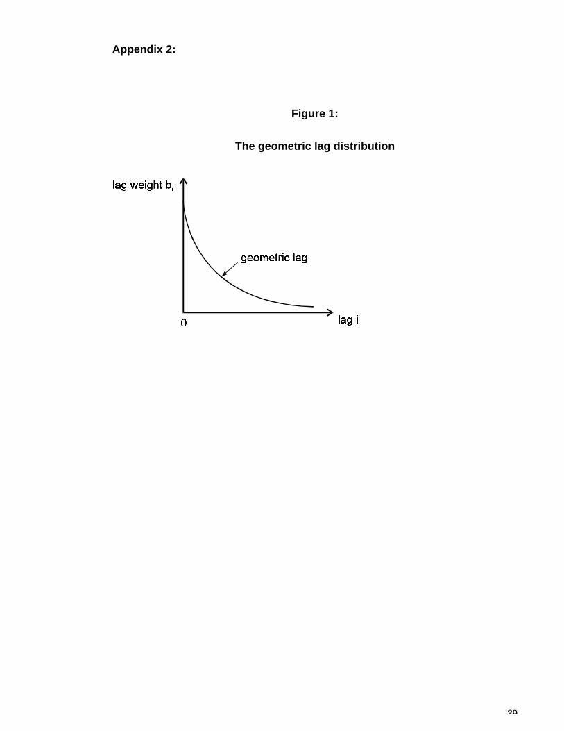
The geometric or Koyck lag model allows for infinite lags thereby avoiding the

problem of how to determine the appropriate lag length. It assumes a

geometrically declining lag structure. Arbitrarily small weights are assigned to the

distant past (see (4’) and (4’’) and figure 1, appendix 2).

(4) xszt = a + bii=

∞∑ 0*rerzt-i + c*dyzt + d*cayzt +ut

(4’) xszt = a + (b0(1- λ ) λ 0)*rerzt +... + (b0(1- λ ) λ ∞)*rerzt- ∞ + c*dyzt + d*cayzt +ut

(4’’) xszt = a + (b0(1- λ )) λi=

∞∑ 0

i*rerzt-i + c*dyzt + d*cayzt + ut

with bi = b0(1- λ ) λ i, i = 0,1,2,...,k and 0 ≤ λ ≤ 1

The equations (4’) and (4’’) have been formulated in moving average form. As it is

well known, they can be transformed into (5), the autoregressive form of the

geometric lag model7, which is best suited to estimation of the partial adjustment

model.

(5) xszt = a’ + b’*rerzt + c’*dyzt + d’*cayzt + λ *xszt-1 + vt

with a’=a(1- λ ); b’=b0=b(1- λ ); c’=c(1- λ ); d’=d(1- λ ) and

vt = (ut - λ ut-1)

12

The following formulas allow us to calculate (Greene, 2000):

(i) The mean lag qav. = λ λ/ ( )1−

(ii) The median lag q* = ln 0.5/ ln λ

(iii) The impact multiplier is b0 = b0*λ 0

(iv) The long run multiplier is bk = b0 λi

k i

=∑ 0;

However, only under the assumption that the disturbance terms are not

autocorrelated, will OLS result in an asymptotically efficient estimator for the

partial adjustment model. Therefore, before applying OLS, a LM test on

autocorrelation must be performed and any problem corrected8 by the FGLS

(Feasible General Least Squares)-technique (Greene, 2000). Although this

is a quite cumbersome procedure, FGLS does generate efficient and

consistent, though biased estimators (Kelejian and Oates, 1981).

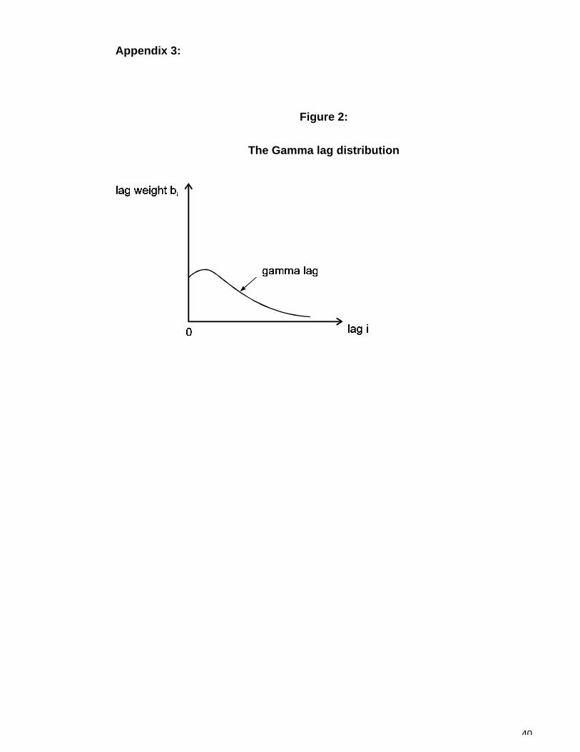
3.2.2 The Gamma lag model

The Gamma lag model is similar to the geometric lag model in that it assumes

infinite lags, thus circumventing the problem of determining the lag length. The

Gamma lag model assumes first a very short increase and then a steadily

declining decrease in the lag structure. That is, if after an initial period (of 1 to 2

years) a declining influence of the real exchange rate on manufacturing exports is

hypothesized, the Gamma lag model becomes relevant. It takes the following

form:

13

(6) xszt = a + b ( )i i

i+

=

∞∑ 10

γ λ * rerzt-i + c* dyzt + d* cayzt + ut

This equation can be transformed into

(7) xszt = a + b* grerzt +η t + c* dyzt + d* cayzt + ut

with 0 ≤ λ p 1; 0p pγ 1; grerzt9 = ( )i

i

t+

=

−∑ 10

1 γ λ i * rerzt-i

and η t = b ( )ii t

+=

∞∑ 1 ( )i +1 γ λ i * rerzt-i → 010

If γ and λ are allowed to take on any value between 0 and 1, the maximum

likelihood estimation of γ , λ ,a, b, c, and d will minimize the sum of squared

errors. Given γ and λ (hence given grerz), the estimation of b is linear. The

procedure is therefore to „search“ over γ and λ , picking those values that

minimize the above sum of squares. The ML (Maximum Likelihood) - method

generates estimators with the desired properties, namely unbiased and efficient

estimators. Alternatively a non-linear least square procedure that relies on an

iterative process might be used (Schmidt, 1974).11

The gamma lag can be described by figure 2 (appendix 3):

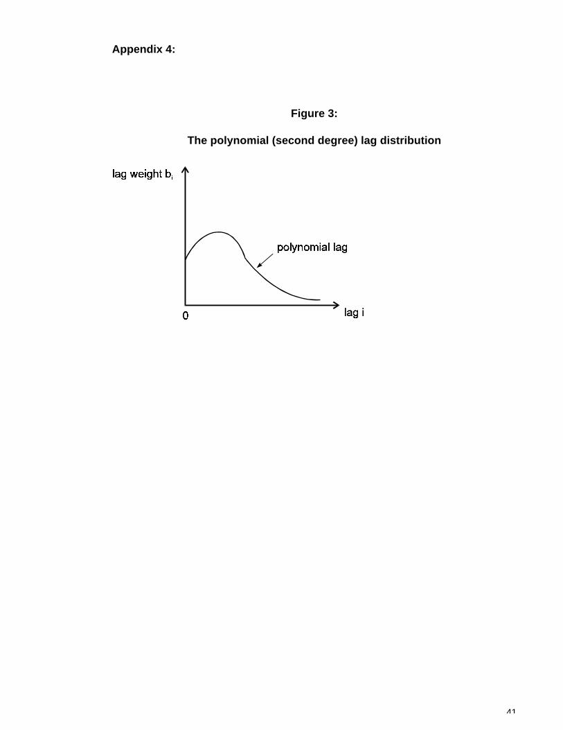
3.2.3 The polynomial lag model

The polynomial lag model (Almon lag model) is a finite lag model. It has two

advantages when compared to the models of 3.2.1(geometric lag model) and

3.2.2 (Gamma lag model): First, in contrast to the geometric lag and the Gamma

lag models which require sophisticated estimation techniques such as FGLS or

ML or non-linear estimation procedures, the polynomial lag model relies on the

OLS-technique. Second, the polynomial lag technique allows one to model any

14

lag structure that can be expressed by a polynomial of degrees 1,...., p (some

finite number).

The major disadvantage of the Almon lag technique is the difficulty of determining

the length and the structure of the lag. The consequences of error in specifying

the lag length and the order of the polynomial are severe. The problem of

misspecifying the lag length and the lag structure is of course aggravated when

monthly or quarterly data are used, because extremely accurate information on

reaction lags would be necessary in order not to miss the true lag length and the

true degree of the polynomial when dealing with monthly or quarterly time-series

(Wohlmann, 1998).

Suppose that economic theory and/or the cross correlations suggest that a

second-degree polynomial is appropriate to describe the form of the lag (see

figure 3, appendix 4).

As it is well known, we would take bi = α α α0 1 22+ +i i (i denoting lag i) and the

polynomial lag model would be of the following form:

(8) xszt = a + α 0 ( rerz t ii

k

−=∑ 0) + α 1 ( i rerz t ii

k* −=∑ 0

) + α 2 ( i rerz t ii

k 2

0* −=∑ )+ c*dyzt

+ d*cayzt + ut

Then the OLS estimators of the b’s (the coefficients of the lagged rerz) could be

calculated according to the following formulas (Kelejian and Oates, 1981):

b0 = α 0

b1 = α α α0 1 2+ +

b2 = α α α0 1 22 4+ +

15

3.2.4 The transfer function model (autoregressive distributed lag model)12

Like the polynomial lag model, the transfer function model (autoregressive

distributed lag model) has the advantage of allowing a great deal of flexibility in

the shape of the lag distribution. However, unlike the polynomial lag model it does

not truncate the distribution at an arbitrarily chosen point and nor does it require

an estimate of the degree of the polynomial (Greene, 2000). Thus misspecification

of lag length and lag distribution can be avoided, making the transfer function

model the model of choice.13

The transfer function model takes the following form:

(9) xszt = µ + A(L)rerzi + c*dyzt + d*cayzt + ut

with A(L) = B(L)/C(L) and α0 ,α1 , α2 ... = the coefficients on 1, L, L2 ,..in

B(L)/C(L) and β i resp. γ i ....= the coefficients on Li in B(L) resp. C(L).

B(L) and C(L) are polynomials in the lag operator. The ratio of the two

polynomials in the lag operator A(L) can produce essentially any desired shape of

the lag distribution with relatively few parameters.14 For example, if both B(L) and

C(L) are quadratic then we get:

(10) xszt = µ (1-γ γ1 2− ) +γ 1*xszt-1 + γ 2 *xszt-2 + β0 *rerzt + β1 *rerzt-1 + β2 *rerzt-2

+c*dyzt - cγ 1*dyzt-1 - cγ 2 *dyzt-2+ d*cayzt -dγ 1*cayzt-1 -dγ 2 *cayzt-2 + (ut- γ 1ut-1-

γ 2 ut-2)

Equation (10) is referred to as an autoregressive distributed lag model with a

moving average (MA) disturbance. It should be noted that OLS estimation, a

16

linear estimation technique, will lead to consistent estimates, but that it can only

be applied when there are no moving average terms.15

When there are moving average disturbances, the model becomes non-linear. In

this case, the non-linear least square estimator will be consistent and

asymptotically normally distributed (Greene, 2000).

For obtaining α0 , α1 and α2 we start from the following relationship: A(L)*C(L) =

B(L).

We get the following formulas:

no lag: α β0 0= = b0

1-period lag: α β α γ1 1 0 1= + = b1

2-period lag: α β α γ α γ2 2 0 2 1 1= + + = b2

3.3 Presentation and discussion of the results

The data requirements were two-fold : First, all variables had to enter the

regression equation in real terms16 (see Appendix 1 for a description of the

variables) . Second, all variables / time-series had to be transformed into

stationary series in order to avoid the problem of running spurious regressions

(Granger and Newbold, 1974, Phillips, 1986 and Darnell 1994). Stationary series

will be characterized by the letter z, generating xsz, rerz, dyz and cayz.

Stationarity of the time series was tested by the Augmented Dickey-Fuller test.

The original time series in levels (XS, RER, DY, CAY) were found to be non-

stationary, but co-integrated (Johansen, 1988 and Darnell 1994). Therefore, a

17

long-run equilibrium between the variables without delays in any explanatory

variable could be assumed.

However, our interest lies in the short-run/medium-run relationship between the

export supply and its macro determinants as well as in the quantification of the

lagged effects. When analysing the short-run/medium run, one wants to control

for time trends in the variables which cause non-stationarity of the series and

spurious regressions. Therefore, the series have to be made stationary. In the

econometric literature two methods are recommended for obtaining stationarity: 1)

regressing the time series as a simple linear (or higher order) function of time and

then using the residuals as the detrended series or 2) utilizing first (or higher)

differences of the time series. However, both methods have severe shortcomings.

Method 1 fails when the time series are generated by a random walk with drift

since the residual would not be stationary. Time series characterized by growth

(such as XS and DY) are quite certainly characterized by a random walk with drift.

The problem concerning method 2 is that it assumes a 100% autocorrelation

between the disturbance terms at any point of time, which will rarely be the case.

Therefore, the author used a third method in order to obtain stationary series. By

this third method the variables are freed from short-run disturbances

(autocorrelation). On the other hand, however, they retain the ability to ‘carry’ all

relevant information.

By applying a simple model without distributed lags (equation (2)), the general

functioning of method 3, which proceeds basically as FGLS (feasible generalized

least squares) shall be demonstrated:

(2) xst = a + b * rert + c * dyt + d * cayt + ut

18

First, a, b, c and d are to be estimated by OLS, provided that the regressors can

be considered as exogenous. Second, the estimated values for a, b, c, and d are

plugged into eq. (2) and then the estimated values (evxst) of xst are calculated.

Third, the estimated values (evut) of ut are calculated according to evut = xst -

evxst. Forth, a simple regression (eq. (2’)), based on a verified first order

autocorrelation, is run:

(2’) evut = ρ * evut-1 + ε t

and ρ is estimated. Fifth, stationary series (xsz, rerz, dyz and cayz) are produced

by removing the autocorrelation part from each variable:

xszt = xst - ρ * xst-1; rerzt, dyzt and cayzt are generated analogically.

The exogenity/endogenity of the variables rerz, dyz and cayz (stationary variables

in LOG-form) was tested in each of the distributed lag models with the Hausman

test.17 The test results were negative. This is to say that the regressors rerz, dyz

and cayz were considered sufficiently exogenous to be estimated by non-TSLS-

methods.

In subsequent steps the distributed lag models were subjected to two further tests:

The Chow Breakpoint tests were applied, assuming structural change in the year

197418. No structural change could be detected for α = 0.05 and α = 0.01 in any

of the models.

The Breusch-Godfrey Serial Correlation LM tests to diagnose autocorrelation

were conducted. These tests were all negative for α = 0.01 and 0.05 indicating

that autocorrelation did not constitute a problem.19

19

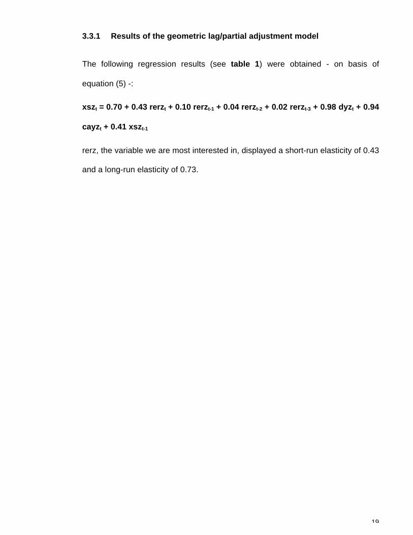
3.3.1 Results of the geometric lag/partial adjustment model

The following regression results (see table 1) were obtained - on basis of

equation (5) -:

xszt = 0.70 + 0.43 rerzt + 0.10 rerzt-1 + 0.04 rerzt-2 + 0.02 rerzt-3 + 0.98 dyzt + 0.94

cayzt + 0.41 xszt-1

rerz, the variable we are most interested in, displayed a short-run elasticity of 0.43

and a long-run elasticity of 0.73.

20

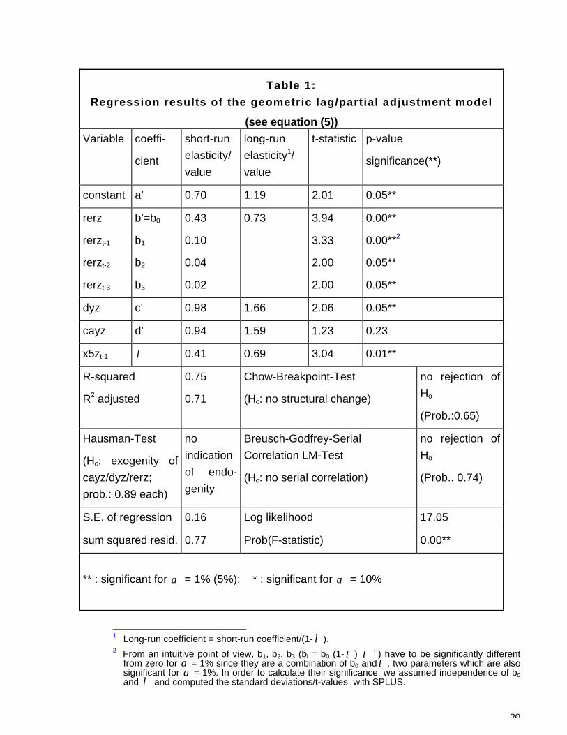
1 Long-run coefficient = short-run coefficient/(1- λ ).2 From an intuitive point of view, b1, b2, b3 (bi = b0 (1- λ ) λ i ) have to be significantly different

from zero for α = 1% since they are a combination of b0 and λ , two parameters which are alsosignificant for α = 1%. In order to calculate their significance, we assumed independence of b0and λ and computed the standard deviations/t-values with SPLUS.

Table 1:

Regression results of the geometric lag/partial adjustment model

(see equation (5))

Variable coeffi-

cient

short-run

elasticity/

value

long-run

elasticity1/

value

t-statistic p-value

significance(**)

constant a’ 0.70 1.19 2.01 0.05**

rerz

rerzt-1

rerzt-2

rerzt-3

b’=b0

b1

b2

b3

0.43

0.10

0.04

0.02

0.73 3.94

3.33

2.00

2.00

0.00**

0.00**2

0.05**

0.05**

dyz c’ 0.98 1.66 2.06 0.05**

cayz d’ 0.94 1.59 1.23 0.23

x5zt-1 λ 0.41 0.69 3.04 0.01**

R-squared

R2 adjusted

0.75

0.71

Chow-Breakpoint-Test

(Ho: no structural change)

no rejection of

Ho

(Prob.:0.65)

Hausman-Test

(Ho: exogenity of

cayz/dyz/rerz;

prob.: 0.89 each)

no

indication

of endo-

genity

Breusch-Godfrey-Serial

Correlation LM-Test

(Ho: no serial correlation)

no rejection of

Ho

(Prob.. 0.74)

S.E. of regression 0.16 Log likelihood 17.05

sum squared resid. 0.77 Prob(F-statistic) 0.00**

** : significant for α = 1% (5%); * : significant for α = 10%

21

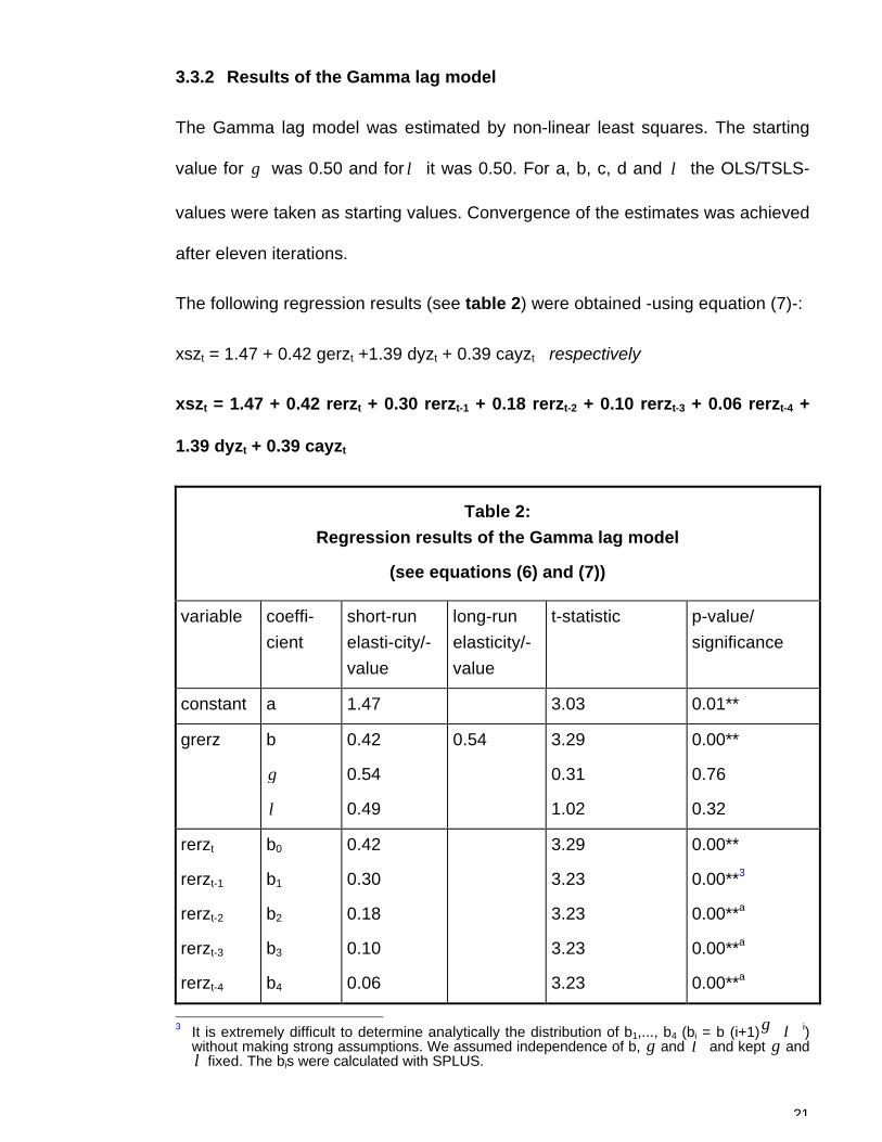
3.3.2 Results of the Gamma lag model

The Gamma lag model was estimated by non-linear least squares. The starting

value for γ was 0.50 and for λ it was 0.50. For a, b, c, d and λ the OLS/TSLS-

values were taken as starting values. Convergence of the estimates was achieved

after eleven iterations.

The following regression results (see table 2) were obtained -using equation (7)-:

xszt = 1.47 + 0.42 gerzt +1.39 dyzt + 0.39 cayzt respectively

xszt = 1.47 + 0.42 rerzt + 0.30 rerzt-1 + 0.18 rerzt-2 + 0.10 rerzt-3 + 0.06 rerzt-4 +

1.39 dyzt + 0.39 cayzt

Table 2:

Regression results of the Gamma lag model

(see equations (6) and (7))

variable coeffi-

cient

short-run

elasti-city/-

value

long-run

elasticity/-

value

t-statistic p-value/

significance

constant a 1.47 3.03 0.01**

grerz b

γ

λ

0.42

0.54

0.49

0.54 3.29

0.31

1.02

0.00**

0.76

0.32

rerzt

rerzt-1

rerzt-2

rerzt-3

rerzt-4

b0

b1

b2

b3

b4

0.42

0.30

0.18

0.10

0.06

3.29

3.23

3.23

3.23

3.23

0.00**

0.00**3

0.00**a

0.00**a

0.00**a

3 It is extremely difficult to determine analytically the distribution of b1,..., b4 (bi = b (i+1)γ λ i)

without making strong assumptions. We assumed independence of b, γ and λ and kept γ andλ fixed. The bis were calculated with SPLUS.

22

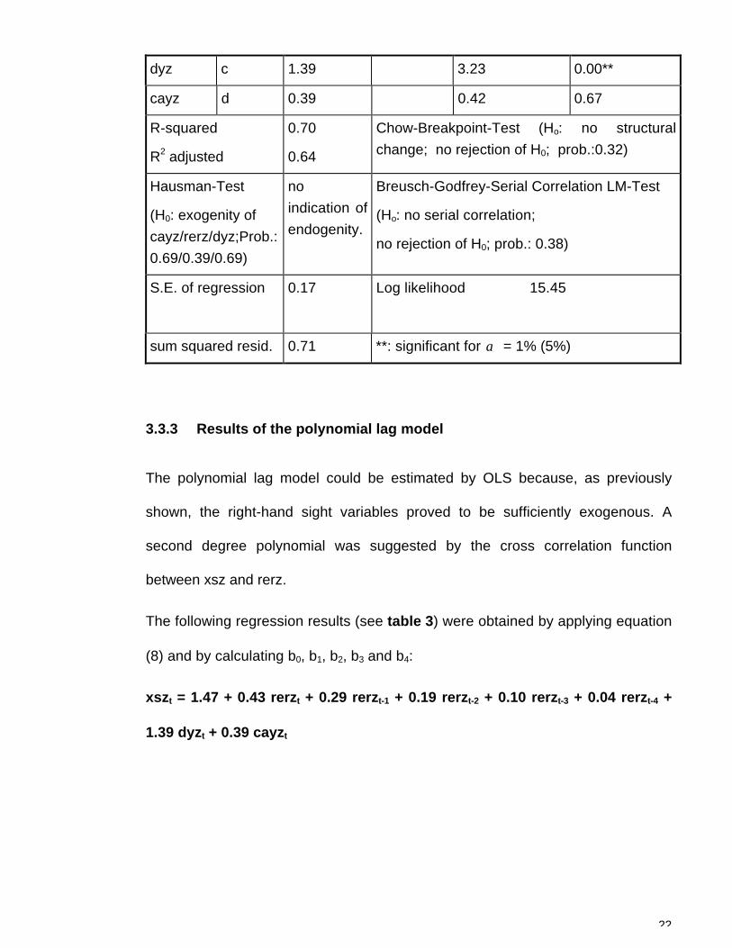
dyz c 1.39 3.23 0.00**

cayz d 0.39 0.42 0.67

R-squared

R2 adjusted

0.70

0.64

Chow-Breakpoint-Test (Ho: no structural

change; no rejection of H0; prob.:0.32)

Hausman-Test

(H0: exogenity of

cayz/rerz/dyz;Prob.:

0.69/0.39/0.69)

no

indication of

endogenity.

Breusch-Godfrey-Serial Correlation LM-Test

(Ho: no serial correlation;

no rejection of H0; prob.: 0.38)

S.E. of regression 0.17 Log likelihood 15.45

sum squared resid. 0.71 **: significant for α = 1% (5%)

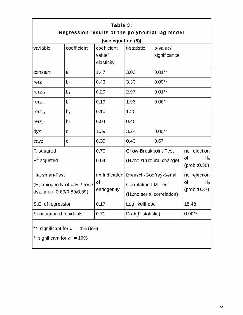
3.3.3 Results of the polynomial lag model

The polynomial lag model could be estimated by OLS because, as previously

shown, the right-hand sight variables proved to be sufficiently exogenous. A

second degree polynomial was suggested by the cross correlation function

between xsz and rerz.

The following regression results (see table 3) were obtained by applying equation

(8) and by calculating b0, b1, b2, b3 and b4:

xszt = 1.47 + 0.43 rerzt + 0.29 rerzt-1 + 0.19 rerzt-2 + 0.10 rerzt-3 + 0.04 rerzt-4 +

1.39 dyzt + 0.39 cayzt

23

Table 3:

Regression results of the polynomial lag model

(see equation (8))

variable coefficient coefficient

value/

elasticity

t-statistic p-value/

significance

constant a 1.47 3.03 0.01**

rerzt b0 0.43 3.33 0.00**

rerzt-1 b1 0.29 2.97 0.01**

rerzt-2 b2 0.19 1.93 0.06*

rerzt-3 b3 0.10 1.20

rerzt-4 b4 0.04 0.40

dyz c 1.39 3.24 0.00**

cayz d 0.39 0.43 0.67

R-squared

R2 adjusted

0.70

0.64

Chow-Breakpoint-Test

(Ho:no structural change)

no rejection

of H0

(prob.:0.30)

Hausman-Test

(Ho: exogenity of cayz/ rerz/

dyz; prob: 0.69/0.89/0.69)

no indication

of

endogenity

Breusch-Godfrey-Serial

Correlation LM-Test

(Ho:no serial correlation)

no rejection

of H0

(prob.:0.37)

S.E. of regression 0.17 Log likelihood 15.48

Sum squared residuals 0.71 Prob(F-statistic) 0.00**

**: significant for α = 1% (5%)

*: significant for α = 10%

24

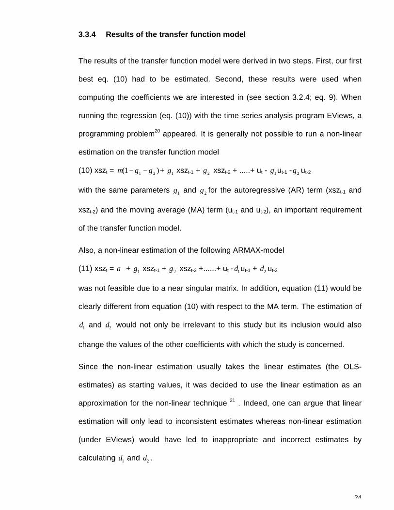
3.3.4 Results of the transfer function model

The results of the transfer function model were derived in two steps. First, our first

best eq. (10) had to be estimated. Second, these results were used when

computing the coefficients we are interested in (see section 3.2.4; eq. 9). When

running the regression (eq. (10)) with the time series analysis program EViews, a

programming problem20 appeared. It is generally not possible to run a non-linear

estimation on the transfer function model

(10) xszt = µ γ γ( )1 1 2− − + γ 1 xszt-1 + γ 2 xszt-2 + .....+ ut - γ 1 ut-1 -γ 2 ut-2

with the same parameters γ 1 and γ 2 for the autoregressive (AR) term (xszt-1 and

xszt-2) and the moving average (MA) term (ut-1 and ut-2), an important requirement

of the transfer function model.

Also, a non-linear estimation of the following ARMAX-model

(11) xszt = α + γ 1 xszt-1 + γ 2 xszt-2 +......+ ut -δ1ut-1 + δ2 ut-2

was not feasible due to a near singular matrix. In addition, equation (11) would be

clearly different from equation (10) with respect to the MA term. The estimation of

δ1 and δ2 would not only be irrelevant to this study but its inclusion would also

change the values of the other coefficients with which the study is concerned.

Since the non-linear estimation usually takes the linear estimates (the OLS-

estimates) as starting values, it was decided to use the linear estimation as an

approximation for the non-linear technique 21 . Indeed, one can argue that linear

estimation will only lead to inconsistent estimates whereas non-linear estimation

(under EViews) would have led to inappropriate and incorrect estimates by

calculating δ1 and δ2 .

25

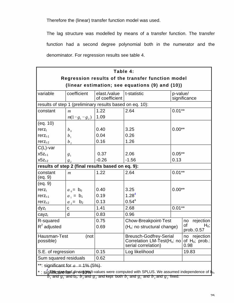
Therefore the (linear) transfer function model was used.

The lag structure was modelled by means of a transfer function. The transfer

function had a second degree polynomial both in the numerator and the

denominator. For regression results see table 4.

4 The standard deviations/t-values were computed with SPLUS. We assumed independence of b0,β1 and γ 1 and b0, β2 and γ 2 and kept both β1 and γ 1 and β2 and γ 2 fixed.

Table 4:

Regression results of the transfer function model

(linear estimation; see equations (9) and (10))

variable coefficient elast./valueof coefficient

t-statistic p-value/significance

results of step 1 (preliminary results based on eq. 10):constant µ

µ γ γ( )1 1 2− −1.221.09

2.64 0.01**

(eq. 10)rerzt

rerzt-1

rerzt-2

β0

β1

β2

0.400.040.16

3.250.261.26

0.00**

C(L)-varx5zt-1

x5zt-2

γ 1

γ 2

0.37-0.26

2.06-1.56

0.05**0.13

results of step 2 (final results based on eq. 9):constant(eq. 9)

µ 1.22 2.64 0.01**

(eq. 9)rerzt

rerzt-1

rerzt-2

α 0 = b0

α1 = b1

α 2 = b2

0.400.190.13

3.251.284

0.54a

0.00**

dyzt c 1.41 2.68 0.01**cayzt d 0.83 0.96R-squaredR2 adjusted

0.750.69

Chow-Breakpoint-Test(Ho: no structural change)

no rejectionof H0;prob.:0.57

Hausman-Test (notpossible)

Breusch-Godfrey-SerialCorrelation LM-Test(Ho: noserial correlation)

no rejectionof H0; prob.:0.98

S.E. of regression 0.15 Log likelihood 19.83Sum squared residuals 0.62

**: significant for α = 1% (5%)

* : significant for α = 10%

26

The following regression equation (compare eq. (10) was estimated in a first step:

xszt = 1.22 (1-0.37+0.26) + 0.37 xszt-1 - 0.26 xszt-2 + 0.40 rerzt + 0.04 rerzt-1 + 0.16

rerzt-2 + 1.41 dyzt + 0.83 cayzt.

For simplicity and analogy with the other three models, the coefficients of the

lagged dyz and cayz are not listed in table 4.

In a second step the parameters A(L), i. e. : b0, b1, b2, of the transfer function

model (compare section 3.2.4; eq. (9)) were calculated according to the relations

(A(L)=B(L)/C(L)) stated in section 3.2.4. Recall that the transfer function model

(eq. (9)) contains the regression coefficients we are interested in. The following

regression equation was obtained:

xszt = 1.22 + 0.40 rerzt + 0.19 rerzt-1 + 0.13 rerzt-2 + 1.41 dyzt + 0.83 cayzt

4. Conclusions

4.1 Conclusions for economic policy making

The regression results (tables 1 to 4) give strong empirical support to the

hypothesis that an increase in the real exchange rate does have an important,

positive impact on manufacturing exports.22 Whereas depreciation is conducive to

an export expansion, appreciation of the real exchange rate will lead to a clear

decrease in exports. The results showing the coefficient of the current real

exchange rate (rerzt) to lie in a range between 0.40 (transfer function model) and

0.43 (geometric lag model, polynomial lag model), indicate quite an elastic

reaction of manufacturing exports to changes in the real exchange rate. The

27

partial adjustment model showed a significant adjustment lag (production lag) of

about 8 months. The long-run elasticity was calculated to be approximately 0.73.

The geometric lag, the Gamma lag, the polynomial lag and the transfer function

model revealed by and large the reaction pattern of exports vis-à-vis exchange

rate changes in the past. The coefficients for rerzt-1 , rerzt-2 (and rerzt-3) were

highly significant in the geometric lag, Gamma lag and the polynomial lag model.

They showed a steadily declining, but visible impact of past changes in the real

exchange rate and point to the importance of establishing and maintaining a

competitive real exchange rate. A common feature of the models was that

production capacity (dyz) was always statistically significant, whereas domestic

expenditures/demand conditions (cayz) never was23. The real exchange rate

(rerz) was positive and highly significant in all distributed lag models forα = 1% .

Since the real exchange rate (of the current period and the two preceding years)

must be considered an important determinant for export decisions, the economic

policy should be carefully calibrated to counter the negative effects of an

appreciated real exchange rate. A 10%-appreciation of the real exchange rate will

cause manufacturing exports to decrease between 4.0% and 4.3% - according to

the models applied (see tables 1 to 4) -. Even past appreciations of the real

exchange rate will have a significant impact on exports. Therefore, a nominal

anchor policy (the Argentinian type in the period of 1991-2001)24 or a currency

peg, such as the pegging of the domestic currency to a currency basket with the

possibility of fluctuation within a certain range (the Chilean type in the period of

1991-1999)25 must be closely monitored whenever the domestic rate of inflation

exceeds that of the pegging partner(s) and appreciation tendencies appear.

28

These results of a positive, significant relationship between export supply and real

exchange rate are not necessarily in line with studies based on quarterly data. For

example, a comparable study by M. Wohlmann (1998) found an insignificant and

unsystematic26 relationship between export supply and real exchange rate. This

phenomenon seems to be caused by a tremendous short-run variability of the

data under consideration. It is extremely difficult to discover the lag structure of

quarterly time series relationships due to seasonal and/or one-time fluctuations in

these data. This problem will persist - even tough in a weaker form - if the data

have been both seasonally adjusted and prewhitened according to Jenkin’s

method before entering the regression equation (Jenkins, 1979).

4.2 Econometric conclusions

The explanatory power (adjusted R-squared) of the four models presented above

lies in the range of 0.64 and 0.71 (see tables 1 to 4). It is highest for the geometric

lag (partial adjustment model) and the transfer function model with 0.71 and 0.69.

The Log-likelihood value of the transfer function model was highest. The

geometric lag model and the Gamma lag model allow the straightforward

calculation of short-run elasticities, long-run elasticities and adjustment lags (i.e.

production lags).

In principle, all models are suited to describe the reaction pattern of export supply

to changes of the real exchange rate of current and past periods. The results

obtained are stable and robust. They give strong statistical support for the

hypothesis that the real exchange rate (rerzt) does have a significant, positive

29

impact on export supply, regardless which model is applied. The coefficients (b1

and b2 ) of rerzt-1 and rerzt-2 were highly significant in the polynomial lag model.

Since in this model the bis are a linear combination of b0 and other parameters,

their standard deviations and corresponding t-values are easy to compute. As far

as the other three models are concerned, one has to keep in mind that the bis are

a non-linear function of b0 and other coefficients, thus making statements

concerning their significance difficult. It is extremely complicated to determine

analytically their distribution. Under certain assumptions (e. g. independence)

SPLUS computed highly significant values for them. However, when the

assumption of normal distribution is not fulfilled, the standard deviations cease to

be a good indicator of 'spread'. This problem might have been present when

calculating the t-value of the bis in the transfer function model.

Nonetheless, the transfer function model has the most desirable properties by

allowing one to shape any lag structure (not only a geometric lag, a Gamma lag

and a polynomial lag structure). In this study cross correlations justify, by and

large, the use of all four models27, however in other cases cross correlation

functions may clearly rule out models with a presumptive form (such as the

models of section 3.2.1, 3.2.2 and 3.2.3). It should also be noted that the transfer

function model was the model with one of the best Durbin-Watson statistics28, if

one is willing to accept this statistic as a rough indicator for model specification.

The study found that EViews had limitations in dealing with the transfer function

model, whereas AUTOBOX, a competing time series analysis program, does not

have problems in handling transfer functions. However, one should avoid „over-

parametrization“ of the transfer function and help AUTOBOX by setting starting

values.29

30

31

Bibliography

Banco Central de Chile. Boletín Mensual. Various Issues. Santiago. Chile.

Banco Central de Chile. Economic and Financial Report . Various Issues.

Santiago. Chile.

Banco Central de Chile. 1995. 69a Memoria Anual 1994. Santiago. Chile.

Beenstock, M., Lavi, Y. and S. Ribon (1994) The Supply and the Demand for

Exports in Israel, Journal of Development Economics, 44, 333-350.

Ceglowski, J. (1997) On the Structural Stability of Trade Equations: The Case of

Japan, Journal of International Money and Finance, 16, 491-512.

Cotsomitis, J., DeBresson, C. and A. Kwan (1991) A Re-examination of the

Technology Gap Theory of Trade: Some Evidence from Time Series Data for

O.E.C.D. Countries, Weltwirtschaftliches Archiv (Review of World

Economics), Band 127, Heft 4, 792-799.

Darnell, A. C. (1994) A Dictionary of Econometrics, Edward Elgar Publishing

Limited, England, USA.

Diewert, W. E. and C. Morrison (1988) Export Supply and Import Demand

Functions: A Production Theory Approach, in Feenstra (ed.) Empirical

Methods for International Trade, MIT Press, Cambridge, MA, 207-229.

Dornbusch, R. (1980) Open Economy Macroeconomics. Basic Books, Inc.

Publishers, New York.

32

Faini, R. (1994) Export Supply, Capacity and Relative Prices, Journal of

Development Economics, 45, 81-100.

Goldstein, M. and M. Khan (1978) The Supply and Demand for Exports: A

Simultaneous Approach, The Review of Economics and Statistics, LX, 275-

286.

Granger, C. and P. Newbold (1974) Spurious Regressions in Econometrics,

Journal of Econometrics, 2, 111-120.

Greene, W. H. (1993) Econometric Analysis, Prentice Hall, New York, 2nd edition.

Greene, W. H. (2000) Econometric Analysis, Prentice Hall, New York, 4th edition,

international edition.

Gregorio de, J. (1984a) La Balanza Comercial Chilena: Un estudio cuantitativo

para el período 1960-81, Tésis, Universidad de Chile, Facultad de Ciencias

Físicas y Matemáticas, Departamento de Ingenería Industrial, Santiago,

Chile.

Gregorio de, J. (1984b) Compartamiento de las exportacines e importaciones en

Chile: Un estudio econométrico, Estudios CIEPLAN, no. 13.

IMF (2000), Annual Report on Exchange Arrangements and Exchange

Restrictions 2000, Interrnational Monatary Fund, Washington D. C.

IMF (2002), Annual Report on Exchange Arrangements and Exchange

Restrictions 2002, Interrnational Monatary Fund, Washington D. C.

International Monetary Fund, International Financial Statistics Yearbook, Various

Issues, Washington, D. C.

33

Jenkins, G. M. (1979) Practical Experiences with Modelling and Forecasting Time

Series. Gwilym Jenkins & Partners (Overseas) Ltd., St. Helier.

Johansen, S. (1988) Statistical Analysis of Cointegration Vectors, Journal of

Economic Dynamics and Control, 12, 231-254.

Junz, H. and R. Rhomberg (1973) Price Competitiveness in Export Trade Among

Industrial Countries, The American Economic Review, 63, 412-418.

Kelejian, H. and W. Oates (1981) Introduction to Econometrics: Principles and

Applications, Harper & Row Publishers, New York.

Khan, M. (1974) Import and Export Demand in Developing Countries, IMF Staff

Papers, 678-693.

Khan, M. and M. Knight (1988) Import Compression and Export Performance in

Developing Countries, The Review of Economics and Statistics, 70, 315-321.

Maddala, G. S. (1977) Econometrics, Mc Graw-Hill, Inc., New York.

Mann, H. and A. Wald (1943) On the Statistical Treatment of Linear Stochastic

Difference Equations, Econometrica, 7, 173-220.

Moreno, L. (1997) The Determinants of Spanish Industrial Exports to the

European Union, Applied Economics, 29, 723-732.

Muscatelli, V., Stevenson, A. and C. Montagna (1995) Modeling Aggregate

Manufactured Exports for Some Asian Newly Industrialized Economies, The

Review of Economics and Statistics, LXXVII, 147-155.

34

Newman, J., Lavy, V. and de Vreyer, P. (1995). Export and Output Supply

Functions with Endogenous Domestic Prices, Journal of International

Economics, 38, 119-141.

Nowak, F. (1989) Auswirkungen der Außenhandels- und Kapitalverkehrs-

liberalisierung auf den realen Wechselkurs und die Produktion von Gütern:

Theoretische Überlegungen und empirische Untersuchungen am Fallbeispiel

Chile, Arbeitsberichte des Ibero-Amerika Instituts für Wirtschaftsforschung

der Universität Göttingen, Nr. 26., Verlag Otto Schwarz & Co., Göttingen.

Nowak-Lehmann D. , F. (1989) The Estimation of Adjustment Lags and of Price

and Income Elasticities within a Macroeconomic Model: The Case of Chile

(1960-86), Ibero-Amerika Institut für Wirtschaftsforschung, University of

Göttingen Diskussionsbeiträge 48 (September).

Peñaloza Webb, R. (1988) Elasticidad de la demanda de las exportaciones: La

experiencia mexicana, Comercio Exterior (México), 38, 381-387.

Phillips, P. (1986) Understanding Spurious Regressions, Journal of Econometrics,

33, 311-340.

Pindyck, R. and D. Rubinfeld (1981) Econometric Models and Economic

Forecasts, Mc Graw-Hill, Inc., New York, Second Edition.

Pindyck, R. and D. Rubinfeld (1991) Econometric Models and Economic

Forecasts. Mc Graw-Hill, Inc.; New York, Third Edition.

Salas, J. (1982) Estimation of the Structure and Elasticities of Mexican Imports in

the Period 1961-1979, Journal of Development Economics, 10, 297-311.

35

Schmidt, P. (1974) An Argument for the Usefulness of the Gamma Distributed Lag

Model, International Economic Review, 15, 246-250.

Sjaastad, L. (1981) Protección y el volumen de comercio: la evidencia, Cuadernos

de Economía No. 54-55 (Pontifica Universidad Católica de Chile), 263-292.

Wohlmann, M. (1998) Der nominale Wechselkurs als Stabilitätsanker. Die

Erfahrungen Argentiniens 1991-1995, Goettinger Studien in Development

Economics, Vol. 5, Vervuert Verlag, Frankfurt am Main.

36

Appendix 1: Description of variables

The data have been taken from statistics of the Banco Central de Chile and the

International Monetary Fund (see bibliography under these headings). The

deflator for manufacturing exports (DEX) has been provided by Erik Haindl

(Universidad de Chile, Departamento de Economía, Santiago de Chile) for the

period 1960 to 1986. Banco Central - deflators (Economic and Financial Report,

various issues) have been used for the remaining years.

The real exchange rate (RER)

The real exchange rate is the actual, nominal exchange rate adjusted for the

relevant price levels at home and abroad. The foreign price level was

approximated by the whole sale price index (WPI) of Chile's main trading partners

and the domestic price index was approximated by the consumer price index

(CPI). This methodology is also used by Chile's Central Bank (compare Banco

Central: Economic and Financial Report of March , 1992, p. 11).

It has to be pointed out that the price indices used do not include export subsidies

or other incentives for exporting and therefore the real effective exchange rate

could not be calculated. However, the real exchange rate was refined by

correcting for the importance of Chile's export trade partners.

Since Chile has export-trade relations with a number of foreign countries of

varying importance, the pairwise bilateral nominal exchange rates and the foreign

WPI’s have to enter the RER-formula according to their export-trade weights. By

37

relying on 14 export-trading partners that make up 80% of Chile’s export-trade,

the RER has been calculated the following way:

RER = ( * / )j

J

CHj j CHwCHJe WPI CPI

=

=

∏1

14

with j=1,......,14 trading partners who make up 80 % of Chile's export trade

eCHj = nominal exchange rate between Chile and trading partner j

WPIj = whole sale price index of trading partner j

CPICH = consumer price index of Chile

wCHj = export trade weight (percentage of Chilean manufacturing exports going to

trading partner j); export trade weights were recalculated for each year and add

up to 1 in each year.

RER is an index value with value 1.00 for the base year 1986.

Trend of Chilean GDP (DY)

DY stands for Chilean trend domestic product (GDP). It is used as an indicator for

capital stock data/production capacity. It is derived from Chilean GDP in real

terms with 1986 as base year.

Chile’s real absorption deficit /surplus30 in relation to real GDP (CAY)

CAY is treated as an indicator for real domestic absorption. It is measured as the

percentage share of a current account deficit/surplus with respect to GDP. CAY

stands for an absorption deficit/surplus, domestic demand conditions (real

expenditures) and eventually expenditure-reducing policies.

38

Manufacturing exports (XS)

The export values are fob-values measured in millions of Pesos of 1986. The

exports registered in millions of US dollars have to be translated into real terms

according to the following formula:

XS = (EX*e/DEX)*100

with

XS = real manufacturing exports in millions of Pesos of 1986

EX = nominal manufacturing exports in millions of US-$

e = nominal exchange rate between Chilean Peso and US-$

DEX = Peso deflator for manufacturing exports with 1986=100

39

Appendix 2:

Figure 1:

The geometric lag distribution

40

Appendix 3:

Figure 2:

The Gamma lag distribution

41

Appendix 4:

Figure 3:

The polynomial (second degree) lag distribution

42

1 Data cover the period of 1960 to 1996, but should be sufficient for the econometric modelling.2 General information on the construction of macroeconomic export models can be found in studies of J. de

Gregorio (1984a and 1984b), M. Goldstein and M. Khan (1978), M. Khan (1974), L. Sjaastad (1981), J.

Salas (1982), R. Penaloza Webb (1988), M. Khan and M. Knight (1988), F. Nowak (1989), F. Nowak-

Lehmann D. (1989), Beenstock et al.(1994), R. Faini (1994), V. Muscatelli et al. (1995), J. Newman et al.

(1995), J. Ceglowski (1997) and L. Moreno (1997).

3 When the impact of RER, DY and CAY is non-separable (in statistical terms), then RER, DY and CAY will

enter the regression equation in a multiplicative way. When the impact of the independent variables is

separable, they will enter the regression equation in an additive way.

4 a is the constant and d belongs to the variable CAY that can not be entered as a LOG-value because it

can take on negative values (income-absorption deficit) for which the LOG is not defined.

5 The data for 1996 (and sometimes for earlier years) are preliminary data. They are estimates which are

based on the available knowledge of the development of the first half of 1996 (or some quarters before

that date).

6 The transfer function model unlike the geometric lag, Gamma lag and polynomial lag models, is not

presumptive in form (see figures 1 to 3).

7 There also exists a moving average form (MA form) of the model. The latter is more robust to

misspecification of autocorrelation of the disturbance, but requires the use of non-linear least squares

(Greene 1993, pp.528-529).

8 If autocorrelation is not corrected, the OLS-estimators will not only be biased, but will not even be

consistent (Kelejian and Oates 1981, p. 160).

9 grerzt (gamma lag transformed „rerz“) is generated by a manipulation which is completely analogous to

the one done in the geometric lag model (Schmidt 1974, p. 247).

10 η t is asymptotically negligible. Therefore, its omission will not affect the asymptotic properties of the

resulting estimates (Schmidt 1974, p.248).

11 This procedure is also available under EViews and leads to consistent estimates. EViews allows the user

to indicate starting values forγ and λ (e.g. 0.5 for each of them) and to indicate the maximum number of

iterations (EViews 4 User’s Guide 2000, pp. 283-285).

43

12 See Jenkins’ detailed presentation of the transfer function model (1979, pp. 38-66).

13 The transfer function model requires information on the number of parameters that should enter the

numerator and the denominator of the transfer function.

14 One should be aware of the problem of „over-parametrization“ which can lead to insignifant and rather

poor results. This issue was discussed with Dave Reilly from AUTOBOX, P.O. Box 563, Hatboro, PA

19040, U.S.A. AUTOBOX is a software that allows automated time series analysis and is a program that

is able to estimate transfer function models. This ability has not been verified and tested by the author

because Autobox is a quite expensive, though powerful program.

15 The assumption of consistency goes back to Mann and Wald (1943) who deducted that under certain

conditions, ordinary, linear least squares estimation and inference procedures were valid asymptotically

Greene (1993, p.540).

16 The main problem when variables have to be calculated in real terms is to find the proper base year and

the proper deflators. Generally the base year has to be a ‘normal’ year with no obvious internal and

external disequilibria. For Chile’s data set ranging from 1960 to 1996 the year 1986 was considered as

base year.

17 The Hausman test could not be performed for the transfer function model.

18 In September 1973 the military regime under A. Pinochet took over. It is assumed that starting in 1974 a

structural change in the economy (change in the structure of the economic models to be applied) might

have taken place. It should be noted that the change in the macroeconomic variables that undoubtedly

occurred cannot be considered as structural change per se.

19 This result is not surprising because the procedure used to generate stationary time series can also be

used for correcting autocorrelation. Therefore, in a sense the model has been corrected for autocorrelation

at the same time that the time series have been made stationary.

20 AUTOBOX is able to handle transfer functions, however not without shortcomings (Autobox' output is

difficult to interpret because Autobox' approach to deal with data totally differs from widely used

statistical/econometric software programs; over-parametrization of the models can lead to strange

results...). Besides, EViews' programming chief (Chris Wilkins) works on fixing the current problems

concerning ARMAX-models.

21 It was confirmed by AUTOBOX (Dave Reilly) that the EViews results would be very similar to the

AUTOBOX results.

44

22 These results are consistent with the export supply elasticity results obtained by Newman et al. (1995) and

Diewert and Morrison (1988) in static models.

23 When real income (gdpz) instead of trend income (dyz) was used, cayz was statistically significant in all

four distributed lag models. This suggests that exports will cease to be dependent on the income-

absorption gap if exporters make long-run investment decisions (inclusion of trend income (dyz) instead of

current real income (gdpz)).

24 The Argentinian peso was fixed with respect to the US-dollar at the ratio 1:1.

25 The Chilean peso was pegged to a currency-basket consisting of the US-dollar (45%), the German mark

(30%) and the Japanese yen (25%).The exchange rate band was set to be +/-10% (Banco Central de

Chile, Memoria Anual 1995, pp.13-14 and p. 33).

26 The regression coefficients would change signs from one quarter to the other.

27 Transfer function models are so advantageous because they are able to shape the lag structure cor-

responding to the data and their cross correlations. The cross correlations hinted at a polynomial lag

structure which can of course be easily modelled by a transfer function.

28 DWgeo= 1.99; DWgam= 1.50; DWpoly= 1.49; DWtrans= 1.9629 The results shown in tables 4 were obtained by using OLS/TSLS starting values and less parameters,

relying on EViews as a second best program.

30 If income-absorption > 0, we talk about an absorption deficit (depressed demand conditions) and if

income-absorption < 0, we talk about an absorption surplus.