Ibero-Amerika Institut für Wirtschaftsforschung Instituto Ibero-Americano de Investigaciones Económicas

Ibero-America Institute for Economic Research (IAI)

Georg-August-Universität Göttingen

(founded in 1737)

Diskussionsbeiträge · Documentos de Trabajo · Discussion Papers

Nr. 140

Problems in Applying Dynamic Panel Data Models: Theoretical and Empirical Findings

Felicitas Nowak-Lehmann D., Dierk Herzer,

Sebastian Vollmer, Inmaculada Martínez-Zarzoso

May 2006

Platz der Göttinger Sieben 3 ⋅ 37073 Goettingen ⋅ Germany ⋅ Phone: +49-(0)551-398172 ⋅ Fax: +49-(0)551-398173

e-mail: uwia@gwdg.de ⋅ http://www.iai.wiwi.uni-goettingen.de

1

Problems in Applying Dynamic Panel Data Models:

Theoretical and Empirical Findings

By

Felicitas Nowak-Lehmann D.: Ibero-America Institute for Economic Research, fnowak@uni-

goettingen.de,

Dierk Herzer : Ibero-America Institute for Economic Research, DierkHerzer@gmx.de

Sebastian Vollmer: Ibero-America Institute for Economic Research,

SebastianVollmer@aol.com

Inmaculada Martínez-Zarzoso: Department of Economics, Applied Economics,

martinei@eco.uji.es

2

Abstract The objective of this paper is twofold: First, the applicability of a widely used dynamic

model, the autoregressive distributed lag model (ARDL), is scrutinized in a panel data setting.

Second, Chile’s development of market shares in the EU market in the period of 1988 to 2002

is then analyzed in this dynamic framework, testing for the impact of price competitiveness on

market shares and searching for estimation methods that allow dealing with the problem of

inter-temporal and cross-section correlation of the disturbances. To estimate the coefficients

of the ARDL model, FGLS is utilized within the Three Stage Feasible Generalized Least

Squares (3SFGLS) and the system Generalized Method of Moments (system GMM) methods.

A computation of errors is added to highlight the susceptibility of the model to problems

related to underlying model assumptions.

Keywords:

dynamic panel data model, autoregressive distributed lag model; pooled 3Stage Feasible

Generalized Least Squares estimation, panel GMM estimation, market shares

JEL: F14, F17, C23

3

Problems in Applying Dynamic Panel Data Models:

Theoretical and Empirical Findings

1. Introduction

In this paper we utilize an autoregressive distributed lag model (ARDL) to estimate the

dynamics of Chile’s market shares in the EU market. This dynamic model has been adapted

from studies of inter alia Balestra and Nerlove (1966), Baltagi and Levin (1986), Arellano and

Bond (1991), Blundell et al. (1992), Islam (1995), Ziliak (1997). Cable (1997) applied an

ARDL to market share behavior and mobility in the UK daily newspaper market. A common

feature of all these studies (and many more studies of this kind) is that the dynamic

relationship between dependent and independent variables is captured by a lagged dependent

variable thus leading to an autoregressive distributed lag models. This is “the” standard

dynamic model that is applied to panel data, as described in Baltagi (2005).

The main aim of this paper is to examine the applicability of the ARDL from a theoretical and

an empirical point of view. From a theoretical point of view, the structure and origin of this

widely used autoregressive distributed lag model are analyzed. From am empirical point of

view estimation problems of the ARDL are illustrated by an empirical application to Chile’s

market shares in the EU market. We distinguish three types of caveats. The first caveat is

related to the theory and refers to the underlying assumptions of the ARDL and the underlying

geometric lag structure. The second caveat deals with the time series properties of the series

and the autocorrelation problem present in most panel data sets. Finally, the third caveat

centers around the endogenity of the lagged dependent variable on the right hand side and the

endogenity of standard instrumental variables in the presence of serial autocorrelation.

The first type of problems arises because the ARDL is derived from a geometric lag (Koyck

lag) model which presumes that all right hand side variables impact on the dependent variable

in exactly this geometric form (Koyck, 1954). The reason for transforming the geometric lag

model into an ARDL is that the geometric lag model is non-linear in its parameters. Non-

linearity in the parameters was considered problematic for estimation in former times.

Nowadays, modern computer software allows one to apply non-linear least squares to the

Koyck-lag model so that this transformation could be regarded as superfluous. Nonetheless,

ARDL continues to be “the” preferred dynamic model since it is so appealing to summarize

the impact of all regressors (lagged and unlagged) in just one variable, namely the lagged

dependent variable! However, derivation of the ARDL from the geometric lag model clarifies

how restrictive the autoregressive ARDL could be.

4

The second type of problems is basically due to non-stationarity of the data entering the panel

analysis. Non-stationarity leads to serial correlation, a problem that has to be dealt with if

present. Panel unit root test and panel autocorrelation test must therefore be applied before

running regressions to check for the presence of autocorrelated disturbances.

The third type of problems arises only when problem 2 applies. In the presence of

autocorrelated error terms additional estimation problems caused by ”derived endogenity”

appear. The lack of exogenity of the lagged dependent variable and/or standard instrumental

variables is the logical consequence of serial correlation. To tackle these estimation problems,

the dynamic panel data model of Chile’s market shares is estimated by both the Three Stage

Least Squares (3SLS) and the Generalized Method of Moments (GMM) in combination with

Feasible Generalized Least Squares (FGLS) to deal with the problem of endogenity and of

autocorrelation of the residuals across cross-sections and over time.

The critical examination of the preconditions, the applicability on panel data and the

problematic nature of ARDL is considered as the main task of the paper and is pursued in

three steps: First, we strive to clarify what it means to have the geometric lag as underlying

lag structure and to outline the conditions under which a transformation from a Koyck-lag

model into an ARDL would be possible. Second, the estimation problems surrounding the

ARDL in the presence of autocorrelated disturbances, taking for granted that the ARDL is the

true model, are discussed and two estimation methods 3SLS and system GMM are proposed.

Third, ARDL is then actually applied to panel data, even though one has to be careful doing

so. This last step is completed with an error analysis.

From an applied economist’s point of view the objective of the paper is to analyze Chile’s

market share in the EU-market on a sectoral level in the period of 1988 to 2002 by applying

panel time-series techniques. The widely used ARDL model is built with six cross-sections

(EU countries) and fifteen annual observations for the seven most important export sectors of

Chile (fish, fruit, wine, ores, wood, pulp of wood and copper). According to this model

market shares are determined by Chile’s and its main competitors’ relative prices in the EU

countries and an unobserved variable, such as strategic behavior. Price competitiveness is

considered a decisive determinant of Chile’s market shares since Chile’s successful export

products are rather homogeneous products (fish, fruit, beverages, ores, copper, and wood and

products thereof).

The paper is set up as follows. In section 2 the derivation of the model and the assumptions of

the ARDL are analyzed and discussed. Section 3 contains some background information on

5

Chile’s market shares in the EU to motivate the model and its empirical application. Section 4

presents the application of the ARDL to Chilean market share data and an error analysis.

Section 5 concludes.

2. Building an ARDL with Panel Market Share Data: Some Caveats

2.1 How to Model Market Shares? Econometric Model Versus Purely Stochastic Model

Following Sutton (2004), there are two contradicting views on the development of market

shares over time: The first goes back to Alfred Chandler and asserts that market shares are

robust over time and that leadership tends to persist for a ‘long’ time. The second view,

propagated by Schumpeter, emphasizes the transience of leadership positions. Schumpeter

labels those positions temporary monopolies created by invention and innovation. However,

there is no benchmark for long or short leadership positions (2002 Japan Conference, 2005).

We will test the relevance of these hypotheses by means of panel unit root tests. If market

shares turn out to be stationary (I(0)), this will indicate that they are robust and persistent

during the period of 1988 to 2002. However, if they result to be non-stationary, then we will

conclude that the Schumpeter hypothesis cannot be rejected by the 1988-2002 data.

There are also two approaches of modeling market shares: According to the first approach,

market shares are basically purely stochastic, according to the second approach market shares

are influenced by hard economic factors such as prices, marketing expenditure, number and

strength of competitors etc. When modeling market shares, Sutton (2004) chooses an eclectic

approach. Favoring the idea of building a stochastic model, he enriches the model by

industry-specific features (e.g. a strategic representation of firms’ competitive responses to

market share changes). However, it has to be kept in mind that strategic behavior is very often

intrinsically unobservable. In contrast to Sutton, we put less emphasis on the stochastic nature

of market shares and stress the role played by sectoral real effective exchange rates that can

be treated as an industry-specific feature. We believe that exchange rates, cost differentials,

tariffs and subsidies are important ‘hard’ factors explaining market shares over time.

Therefore, we will build a dynamic econometric model in which price competitiveness is

considered as decisive for the competitive position. Since strategic behavior is difficult to

model, we assume that strategic behavior and sector-specific characteristics are incorporated

in the residuals of the regression model.

6

2.2 The Dynamic Econometric Market Share Model: The ARDL and the Restrictiveness

of its Assumptions

An autoregressive distributed lag model will be utilized as dynamic model. Since this model

serves as standard dynamic model in panel data analysis, its (general) applicability will be

carefully scrutinized. Our objective is to discuss the preconditions for its applicability and its

limitations by deriving this model. The ARDL approach has been applied in a multitude of

cases and to diverse issues, such as the dynamic demand for natural gas, the dynamic demand

for drug-like products, such as cigarettes, a dynamic model of employment, a dynamic model

for growth convergence, a dynamic lifecycle labor supply model or a dynamic gravity model

(see Balestra and Nerlove (1966), Baltagi and Levin (1986), Arellano and Bond (1991),

Blundell et al. (1992), Islam (1995), Ziliak (1997), Kim et al. (2003)). Finally, it has also been

applied to market share behavior by Cables (1997).

Cable (1997) proposes to model market shares using an autoregressive distributive lag model

(ARDL)1. He selects a first order autoregressive model with a 1-period lagged endogenous

variable2, in which prices and advertising share are the explanatory variables for UK’s

national daily newspapers.

We utilize and modify this model in the following way: Chile’s market share in a specific

sector is determined by Chile’s price advantage (in terms of EU-Chilean producer prices and

EU protection) and Chile’s competitors price advantage in the EU market. In this model,

changes in the real effective exchange rate in the more distant past have a smaller impact on

changes in market shares than exchange rate changes of the more recent past. This assumption

can be very plausible, but must be verified by the underlying data. As will be shown this

model originates from a geometric lag model (Equation (1)) and enables one to model the

reaction of market shares in the short, medium and long run. The lag length is expressed by k

in our model.

Chile’s market share in country i in sector s at time t in the geometric lag approach is

modelled using a log-log-specification:

l (1) istkistk

istkistk

istisist lreerlreerlreerlreershw µλγλγλβλβα +++++++= −− *...*... 00

000

0

where

ive distributed lag models: the geometric lag model and the transfer function model, also known as ARMAX model (for a good description see Greene, 2000)

1 First order autoregressive model. 2 There are two types of autoregress

7

i = 1, 2,…, 6 represents the cross-sections: FRA, NDL, DEU, ITA, GBR and ESP (according

is Chile’s

, we obtain a maximum of 6 cross-sections and 15

ears, resulting in a maximum of 90 observations per sector. The number of observations

to World Bank abbreviations);

t = 1988, 1989, …, 2002 are years (annual observations)

s = 03, 08, 22, 26, 44, 47 and 74 are the sectors (according to the two digit HS classification)

lshwist stands for Chile’s market share in EU country i in sector s at point t. istlreer

real effective exchange rate, prevailing in country i and in sector s and istlreer * is Chile’s

competitor (*) real effective exchange rate, prevailing in country i and in sector s.

Market shares in a specific sector (s) are computed as ratio of Chile’s sectoral exports (X in

the numerator) and EU country i’s imports from the world M.i = MEU+Mnon-EU (in the

denominator). Due to unsubstantial trade volumes, we consider only Chile’s market shares in

France (FRA), the Netherlands (NDL), Germany (DEU), Italy (ITA), UK (GBR), and Spain

(ESP). Market shares are computed for seven sectors at the two-digit HS chapters, namely

fish (03), fruit (08), beverages (22), ores (26), wood (44), pulp of wood (47) and copper (74).

Sources of the data and generation of the data are described in Appendix 1. The period

covered goes from 1988 to 2002. Thus

y

varies depending on the sector studied.

As to the coefficients and the disturbance in this type of model it is assumed that: 0 1pp λ

and that λ is the sa for all regressors. Having the same me λ for all the regressors we can

transform eq. (1) into an autoregressive distributed lag model, otherwise this will not be

possible. Besides, if λ is the same l re, lag length k must be the same for al gressors, too (see

Figure 1).

It is furthermore assumed that iβ = 0βiλ , iγ = 0γ λ i and istµ ~N(0; 2

µσ ).

A model that follows the above-mentioned restrictions can be transformed into the so-called

first order autoregressive model which is characterized by a lagged endogenous variable on

n Nowak-Lehmann D.,

2004).

By lagging eq. (1) by 1 period, multiplying through with

the right hand side (see Kelejian and Oates, 1981; Gree e, 2000 and

λ we obtain

(1’) λµλγ

λγλβλβλαλ

111

0

11

011

011

01

−−−+

−−−+

−−

++

+++++=

istkistk

istkistk

istisist

lreer

lreerlreerlreerlshw

*

...*...

8

By substracting (1’) from (1) and by suppressing and

since both terms become very, very small with large k, we obtain an

autoregressive distributed lag model (eq. (2)) which is very similar to the partial adjustment

model

11

0 −−+

kistk lreerλβ

11

0 −−+

kistk lreer *λγ

3 (Kim et al., 2003):

lshwist = + is*α is0β lreerist + is0γ lreer*ist + isλ lshwist-1 + vist (2)

with = is*α )( λα −1is and vist = istµ -λ 1−istµ following a normal distribution N(0; ). 2

vσ

However, if λ becomes relatively large (say λ = 0.9) and if the lag length k is short (say k =

2), suppression of the above-mentioned terms turns out to be very problematic since about 70

% (i.e. 0.93) of the impact of the lagged variables would be neglected. This will be shown in

detail in section 4.1 and 4.2 in tables 4 and 6 which contain the error analysis.

A short lag length might constitute a problem when working with annual data, but might be of

minor importance when working with monthly or daily data where the lag length is usually

larger.

Besides and most important, eq. (2) is very restrictive, since the underlying model is a

geometric lag model (eq. (1)) which is known to be of the following form.

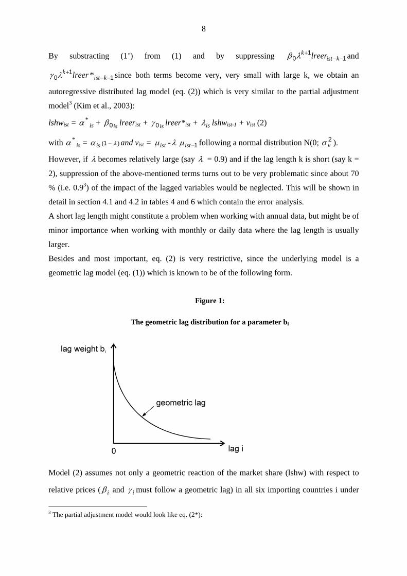
Figure 1:

The geometric lag distribution for a parameter bi

Model (2) assumes not only a geometric reaction of the market share (lshw) with respect to

relative prices ( and iβ iγ must follow a geometric lag) in all six importing countries i under

3 The partial adjustment model would look like eq. (2*):

9

investigation, but it assumes exactly the same (as measured by iλ ) geometric reaction of lshw

with respect to changes of all the regressors (both lreer and lreer*). In our case, as well as in

many other studies using the ARDL, this assumption cannot be justified by the data for all

regressors. Also, this specific geometric reaction does not always apply to all countries under

study. These issues become even more crucial when the number of cross-sections gets bigger

and when we have some more explanatory variables in the model (a model with e.g. 100

countries and 5 regressors).

Moreover, there are many instances in which the assumption of a geometric lag itself will not

be fulfilled. This will be especially the case when reaction lags are present and when therefore

the impact of changes in the current and the preceding periods is smaller than the impact of

changes of earlier periods. In those cases the dynamic model chosen should be a polynomial

lag model which allows one to estimate any lag structure that can be depicted by a polynomial

of order 1, 2,…, p.

Therefore, before applying model (1) or its linear transformation (2) the existence of a

geometric relationship of the coefficients of the independent variables must be scrutinized

very carefully. Incompatibility of the model assumptions with the data will necessarily lead to

inconsistent estimates.

The question that remains unanswered is whether it is more convenient to estimate eq. (1), the

more general geometric lag model, rather than eq. (2), the restricted model. As stated above,

Eq. (1) is non-linear in its parameters, but can be estimated by Non-linear Least Squares

(NLS). By estimating eq. (1) with Non-Linear Least Squares (NLS) together with SUR and

FGLS one will obtain unbiased and efficient estimates if the relative prices (lreer and lreer*)

are exogenous. That is eq. (1) involves no additional estimation problems (beyond the cross-

section and serial correlation) since endogenity of the right hand side variables does not arise

if lreer and lreer* are exogenous. However, Eq. (1) and eq. (2) have in common that the

assumption of a geometric lag must be fulfilled. Non-fulfillment of this assumption will lead

to biased estimates in both models.

2.3 Estimation Techniques for Non-Stationary Panel Data in an ARDL

Assuming for the moment that the underlying assumptions with respect to the geometric lag

of the ARDL model are fulfilled, the time series properties of the series should be checked

λ is0β is0λγ isλλ isαlshwist = + lreerist + lreer*ist + (1- )lshwist-1 + vist; Here it is assumed that the

adjustment to the desired equilibrium level of market share follows a geometric lag.

10

and a test of autocorrelation of the disturbances should be applied. We proceeded in several

steps:

First, we test the time series properties of the data (all in natural logs). All series, i.e. market

shares (lshw), Chile’s real effective exchange rate (lreer) and Chile’s competitors’ real

effective exchange rates (lreer*) for all country-pairs are subject to tests on non-stationarity

(panel unit root tests) in a first step. This procedure is applied to all seven sectors under

investigation. The possible existence of structural breaks in the series is neglected because

neither fundamental, abrupt changes in economic policy nor tremendous exogenous shocks

could be detected in the period of 1988-2002. The governments of Aylwin, Frei and Lagos

continued the economic policy of the Pinochet government. Consequently, the time series

display no sign of a significant structural shift.

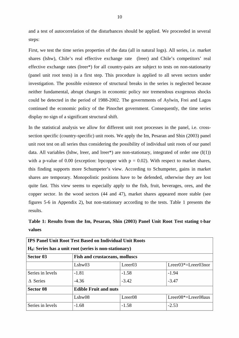
In the statistical analysis we allow for different unit root processes in the panel, i.e. cross-

section specific (country-specific) unit roots. We apply the Im, Pesaran and Shin (2003) panel

unit root test on all series thus considering the possibility of individual unit roots of our panel

data. All variables (lshw, lreer, and lreer*) are non-stationary, integrated of order one (I(1))

with a p-value of 0.00 (exception: lrpcopper with p = 0.02). With respect to market shares,

this finding supports more Schumpeter’s view. According to Schumpeter, gains in market

shares are temporary. Monopolistic positions have to be defended, otherwise they are lost

quite fast. This view seems to especially apply to the fish, fruit, beverages, ores, and the

copper sector. In the wood sectors (44 and 47), market shares appeared more stable (see

figures 5-6 in Appendix 2), but non-stationary according to the tests. Table 1 presents the

results.

Table 1: Results from the Im, Pesaran, Shin (2003) Panel Unit Root Test stating t-bar

values

IPS Panel Unit Root Test Based on Individual Unit Roots

H0: Series has a unit root (series is non-stationary)

Sector 03 Fish and crustaceans, molluscs

Lshw03 Lreer03 Lreer03*=Lreer03nor

Series in levels

∆ Series

-1.81

-4.36

-1.58

-3.42

-1.94

-3.47

Sector 08 Edible Fruit and nuts

Lshw08 Lreer08 Lreer08*=Lreer08aus

Series in levels -1.68 -1.58 -2.53

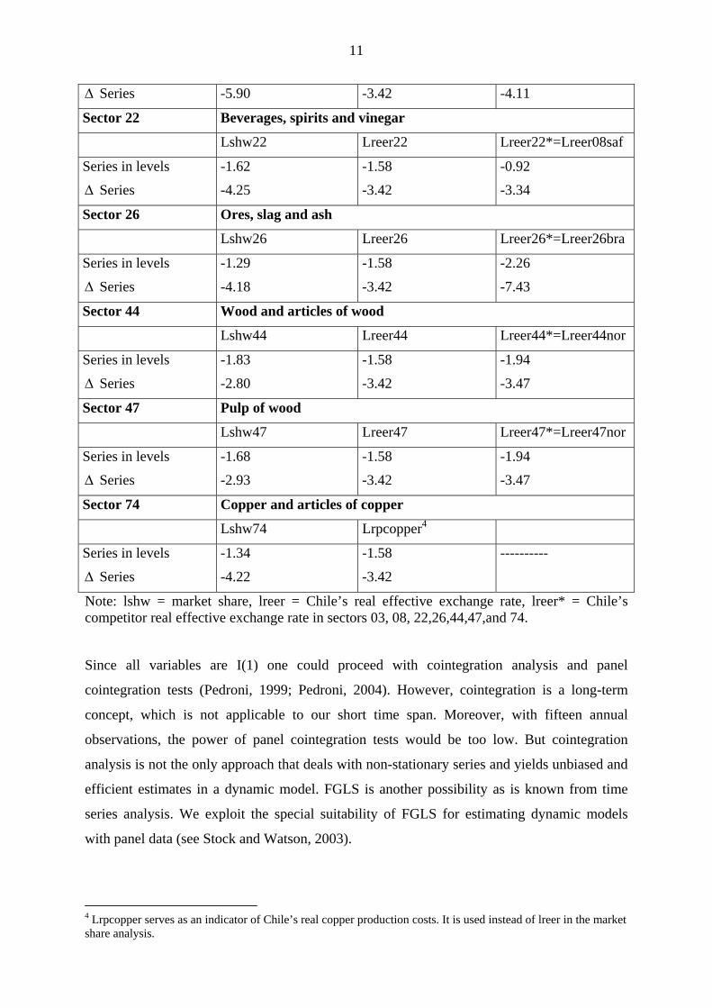
11

∆ Series -5.90 -3.42 -4.11

Sector 22 Beverages, spirits and vinegar

Lshw22 Lreer22 Lreer22*=Lreer08saf

Series in levels

∆ Series

-1.62

-4.25

-1.58

-3.42

-0.92

-3.34

Sector 26 Ores, slag and ash

Lshw26 Lreer26 Lreer26*=Lreer26bra

Series in levels

∆ Series

-1.29

-4.18

-1.58

-3.42

-2.26

-7.43

Sector 44 Wood and articles of wood

Lshw44 Lreer44 Lreer44*=Lreer44nor

Series in levels

∆ Series

-1.83

-2.80

-1.58

-3.42

-1.94

-3.47

Sector 47 Pulp of wood

Lshw47 Lreer47 Lreer47*=Lreer47nor

Series in levels

∆ Series

-1.68

-2.93

-1.58

-3.42

-1.94

-3.47

Sector 74 Copper and articles of copper

Lshw74 Lrpcopper4

Series in levels

∆ Series

-1.34

-4.22

-1.58

-3.42

----------

Note: lshw = market share, lreer = Chile’s real effective exchange rate, lreer* = Chile’s competitor real effective exchange rate in sectors 03, 08, 22,26,44,47,and 74.

Since all variables are I(1) one could proceed with cointegration analysis and panel

cointegration tests (Pedroni, 1999; Pedroni, 2004). However, cointegration is a long-term

concept, which is not applicable to our short time span. Moreover, with fifteen annual

observations, the power of panel cointegration tests would be too low. But cointegration

analysis is not the only approach that deals with non-stationary series and yields unbiased and

efficient estimates in a dynamic model. FGLS is another possibility as is known from time

series analysis. We exploit the special suitability of FGLS for estimating dynamic models

with panel data (see Stock and Watson, 2003).

4 Lrpcopper serves as an indicator of Chile’s real copper production costs. It is used instead of lreer in the market share analysis.

12

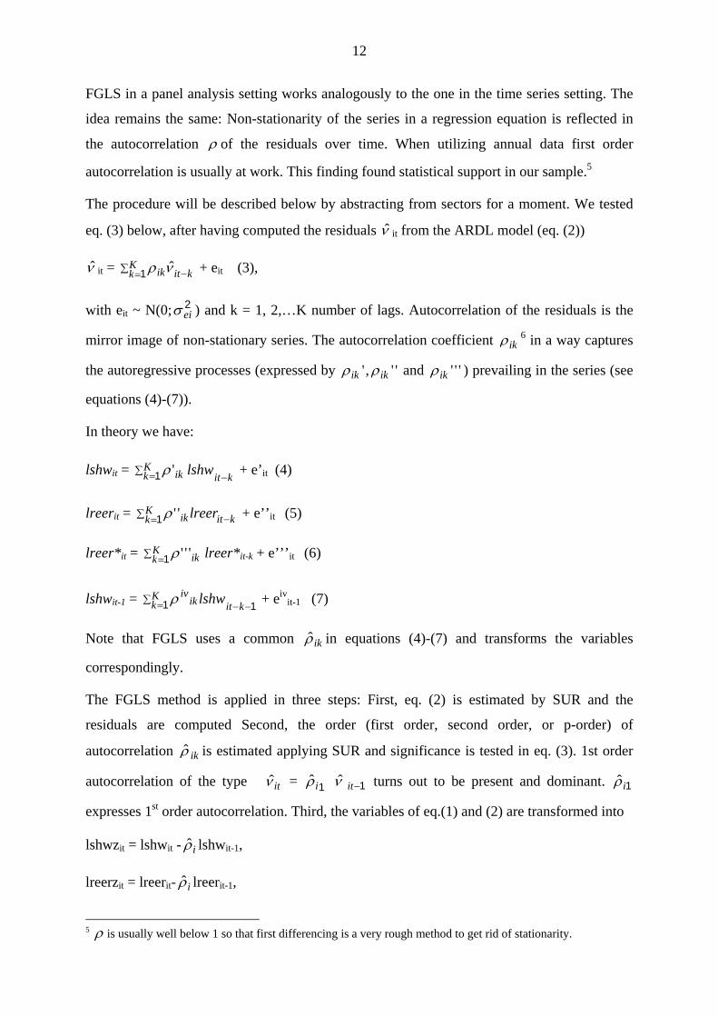
FGLS in a panel analysis setting works analogously to the one in the time series setting. The

idea remains the same: Non-stationarity of the series in a regression equation is reflected in

the autocorrelation ρ of the residuals over time. When utilizing annual data first order

autocorrelation is usually at work. This finding found statistical support in our sample.5

The procedure will be described below by abstracting from sectors for a moment. We tested

eq. (3) below, after having computed the residuals ν̂ it from the ARDL model (eq. (2))

ν̂ it = + ekitKk ik −∑ = νρ ˆ1 it (3),

with eit ~ N(0; ) and k = 1, 2,…K number of lags. Autocorrelation of the residuals is the

mirror image of non-stationary series. The autocorrelation coefficient

2eiσ

ikρ 6 in a way captures

the autoregressive processes (expressed by '',' ikik ρρ and '''ikρ ) prevailing in the series (see

equations (4)-(7)).

In theory we have:

lshwit = + e’kitKk ik lshw

−∑ =1 'ρ it (4)

lreerit = + e’’kitKk ik lreer −∑ =1 ''ρ it (5)

lreer*it = lreer*∑ =Kk ik1 '''ρ it-k + e’’’it (6)

lshwit-1 = + e11 −−∑ = kit

Kk ik

iv lshwρ ivit-1 (7)

Note that FGLS uses a common ikρ̂ in equations (4)-(7) and transforms the variables

correspondingly.

The FGLS method is applied in three steps: First, eq. (2) is estimated by SUR and the

residuals are computed Second, the order (first order, second order, or p-order) of

autocorrelation ikρ̂ is estimated applying SUR and significance is tested in eq. (3). 1st order

autocorrelation of the type itν̂ = 1iρ̂ ν̂ 1−it turns out to be present and dominant. 1iρ̂

expresses 1st order autocorrelation. Third, the variables of eq.(1) and (2) are transformed into

lshwzit = lshwit - iρ̂ lshwit-1,

lreerzit = lreerit- iρ̂ lreerit-1,

5 ρ is usually well below 1 so that first differencing is a very rough method to get rid of stationarity.

13

lreerzit* = lreerit*- iρ̂ lreerit-1*,

lshwzit-1 = lshwit-1- iρ̂ lshwit-2 and

itε = itν̂ - iρ̂ 1−itν̂

thus generating variables in soft or quasi first differences. Eq. (2) is then estimated on basis of

the transformed variables applying SUR (see Stock and Watson, 2003).

In contrast to the dynamic panel analysis literature (Baltagi, 2005), we stress the time series

properties of the series more than it is usually done. The dynamic panel analysis literature

usually abstracts from autocorrelation of the disturbances in order to elaborate more on the

characteristics of one-way error or two-way error component models in which cross-section

specific and time-specific random effects are present.

We take a different route for several reasons: First, we decide to work with a fixed effects

model since our cross-sections are not randomly drawn, but selected on purpose. Second, we

try to account for time series properties because our time dimension exceeds our cross-section

dimension and therefore time series problems should obtain more weight.

Even though serial correlation in dynamic panel data models is only rarely dealt with in the

econometric literature, the studies by Hujer et. al. (2005), Kim et al. (2003), Sevestre and

Trognon (1996) and Keane and Runkle (1992) dwell on this issue. Keane and Runkle (1992)

and Kim et al. (2003) use the forward filtering 2SLS method (KR estimate), which treats

unknown serial correlation in residual disturbance. This method pretends serial correlation to

be one, which is a very rough estimate. Kim et al. (2003) refine the KR method and work with

the variables in first differences. We, in contrast, estimate the extent of serial correlation in

the sample (our )ikρ̂ 7and then transform the variables correspondingly (in soft or quasi first

differences). Hujer et al. (2005) assume that the residual term follows a moving average

process (eg. MA(1), MA(2)). According to our data however, the residual term follows clearly

an AR(1) process and not an MA(1) process. Panel analyses with macroeconomic data usually

show unit-roots in the series and usually show an autoregressive error process. Therefore,

time series tests on the series and the residuals are a must before starting estimation of the

model.

The AR-error structure has severe consequences on the endogenity of the instruments that can

be used in the 3SLS and the GMM routine. These considerations lead us to an alternative

6 Which is to be estimated since it is unknown.

14

method of dealing with non-stationary series in a panel regression framework, namely to

FGLS estimation techniques in combination with 3SLS and a GMM with self-selected

instruments. Before interpreting the regression results we will present some facts on Chile’s

market shares for its most important export sectors and emphasize the role of EU and extra-

EU competition. For each sector separate panel ARDLs will be run over the time period of

1988 to 2002, with the EU countries acting as cross-sections in the panel analysis.

3. Economic Background to the Dynamic Model:

3.1 Chile’s Sectoral Market Shares in a Highly Competitive EU Market

Based on 2003 data, the EU is Chile’s first world-wide trading partner. 25% of Chile’s

exports go to the EU and 19% of its imports come from the EU. During the first semester of

2003, mining (predominantly copper) still represented 46% of total Chilean goods exports,

while agriculture, farming, forestry and fishing products represented 13.02%. Trade with

Chile represents 0.45% of total EU trade, placing Chile as 41st in the ranking of EU main

trading partners. Between 1980 and 2002, EU imports from Chile increased from EUR 1.5

billion to EUR 4.8 billion, whilst EU exports to Chile increased from EUR 0.7 billion to EUR

3.1 billion (EU Commission, 2005).

Given the importance of the EU market to the Chilean export industry, Chile was eager to

sign a Free Trade Agreement (FTA) with the EU (3 October 2002) in order to improve its

market access to the EU. From Chile’s point of view, the agreement can be clearly considered

as a means to maintain and/or strengthen its competitive position in the EU market. In the

short run, a reduction or elimination of trade barriers through a FTA and its impact on relative

prices will improve Chile’s competitive position not only with respect to the EU countries but

also with respect to third countries which do not have a FTA with the EU. In the medium to

long run however, the effect of the FTA will be eroded if the EU decides to conclude also

FTAs with e.g. the MERCOSUR’s full members and perhaps some Asian countries.

Given that Chile’s main export commodities comprise copper, fish, fruits, paper and pulp, and

wine and are thus heavily natural resource based, Chile’s actual competitors are already

numerous8: Norway, Russia, Indonesia, Malaysia, the Philippines and Thailand are much like

Chile exporters of timber and rubber. Besides, the South East Asian countries were able to

7 In FGLS the unknown serial correlation coefficient is estimated as described in section 2. 8 Even though Chile can still be considered the most competitive and the least corrupted economy in Latin America.

15

strongly increase their light manufactured exports to industrial countries in the last decade.

South Africa, Australia and New Zealand, in the Southern Hemisphere, threaten Chile’s

position as a successful fruit and wine exporter. As far as agricultural products are concerned,

Chile faces stiff competition from the EU countries. UK, Ireland and Norway are Chile’s

main competitors as far as fish exports are concerned. Moreover, China, enjoying low labor

costs, has become a strong exporter of machinery and equipment, textiles and clothing,

footwear, toys and sporting goods and mineral fuels, thus reversing in general terms Latin

America’s competitiveness in textile, clothing and shoe exports. When analyzing the

determination of market shares (section 4, Eq. (2)) we will take account of EU and extra-EU

competition.

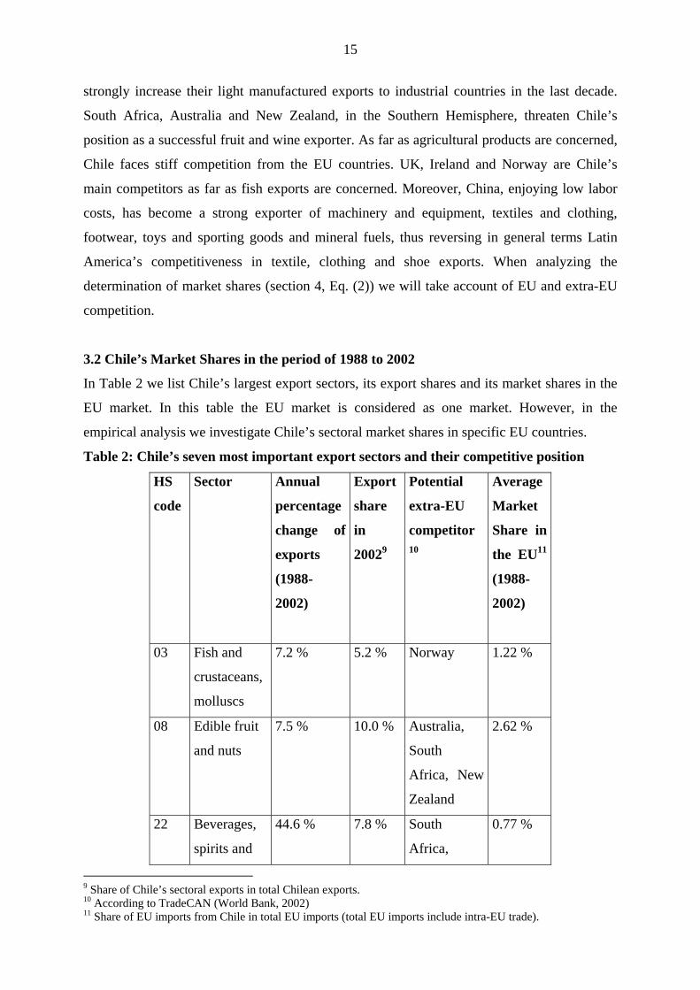
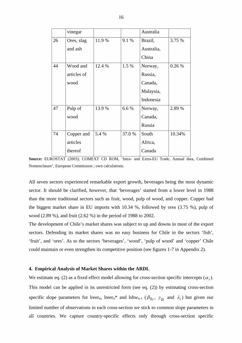
3.2 Chile’s Market Shares in the period of 1988 to 2002

In Table 2 we list Chile’s largest export sectors, its export shares and its market shares in the

EU market. In this table the EU market is considered as one market. However, in the

empirical analysis we investigate Chile’s sectoral market shares in specific EU countries.

Table 2: Chile’s seven most important export sectors and their competitive position

HS

code

Sector Annual

percentage

change of

exports

(1988-

2002)

Export

share

in

20029

Potential

extra-EU

competitor10

Average

Market

Share in

the EU11

(1988-

2002)

03 Fish and

crustaceans,

molluscs

7.2 % 5.2 % Norway 1.22 %

08 Edible fruit

and nuts

7.5 % 10.0 % Australia,

South

Africa, New

Zealand

2.62 %

22 Beverages,

spirits and

44.6 % 7.8 % South

Africa,

0.77 %

9 Share of Chile’s sectoral exports in total Chilean exports. 10 According to TradeCAN (World Bank, 2002) 11 Share of EU imports from Chile in total EU imports (total EU imports include intra-EU trade).

16

vinegar Australia

26 Ores, slag

and ash

11.9 % 9.1 % Brazil,

Australia,

China

3.75 %

44 Wood and

articles of

wood

12.4 % 1.5 % Norway,

Russia,

Canada,

Malaysia,

Indonesia

0.26 %

47 Pulp of

wood

13.9 % 6.6 % Norway,

Canada,

Russia

2.89 %

74 Copper and

articles

thereof

5.4 % 37.0 % South

Africa,

Canada

10.34%

Source: EUROSTAT (2003); COMEXT CD ROM, ‘Intra- and Extra-EU Trade, Annual data, Combined

Nomenclature’, European Commission ; own calculations.

All seven sectors experienced remarkable export growth, beverages being the most dynamic

sector. It should be clarified, however, that ‘beverages’ started from a lower level in 1988

than the more traditional sectors such as fruit, wood, pulp of wood, and copper. Copper had

the biggest market share in EU imports with 10.34 %, followed by ores (3.75 %), pulp of

wood (2.89 %), and fruit (2.62 %) in the period of 1988 to 2002.

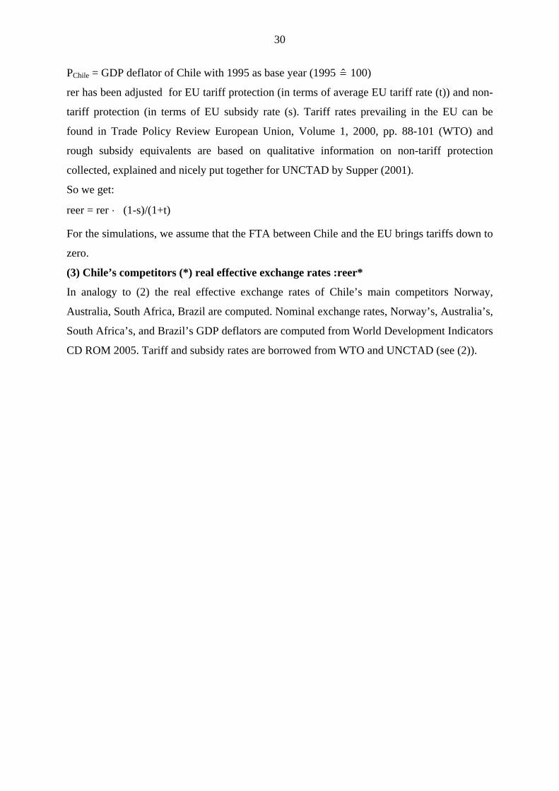
The development of Chile’s market shares was subject to up and downs in most of the export

sectors. Defending its market shares was no easy business for Chile in the sectors ‘fish’,

‘fruit’, and ‘ores’. As to the sectors ‘beverages’, ‘wood’, ‘pulp of wood’ and ‘copper’ Chile

could maintain or even strengthen its competitive position (see figures 1-7 in Appendix 2).

4. Empirical Analysis of Market Shares within the ARDL

We estimate eq. (2) as a fixed effect model allowing for cross-section specific intercepts ( iα ).

This model can be applied in its unrestricted form (see eq. (2)) by estimating cross-section

specific slope parameters for lreerit, lreerit* and lshwit-1 ( i0β , and i0γ iλ ) but given our

limited number of observations in each cross-section we stick to common slope parameters in

all countries. We capture country-specific effects only through cross-section specific

17

intercepts ( iα ) and try to save degrees of freedom by modeling common slope parameters

( 0β , 0γ and λ ) thus estimating eq. (8) for each of the seven sectors:

lshwit = iα + 0β lreerit + 0γ lreer*it + λ lshwit-1 + vit (8)

However, as we have seen before, the advantage of having a linear model is at the cost of

having a lagged endogenous variable that is correlated with the disturbance term due to

autocorrelation. When a lagged endogenous variable appears at the right hand side of a

regression equation (as in the geometric lag model of eq. (2) or eq. (8)) and when the

disturbances are autocorrelated (see eq. (3)), the lagged endogenous variable will be

automatically correlated with the disturbance term and thus becomes endogenous. The

endogenity problem of the lagged dependent variable (lshwit-1), which is caused by first order

AR-correlation of the residuals due to non-stationarity of the series, requires either the use of

the Three-Stage Least Squares12 or the use of the GMM (Generalized Method of Moments)

technique. Modern computer programs allow one to generate the variables in soft first

differences directly by adding e.g. an AR(1) term for first order autocorrelation and to

simultaneously apply methods that control for the endogeneity of the regressors.

4.1 Estimating the Impact of Price Competition on Market Shares Utilizing the 3SLS

Approach in the ARDL model

The choice of instruments is crucial for getting consistent estimates in any model, also in the

market share model. We used an indicator of production capacity in real terms as an

instrument for lagged market share (lshwit-1), the difference in PPP-income between Chile and

the importing country as an instrument for lreerit, and the competitor’s real exchange rate in a

transformation that is generally used in polynomial lag models as an instrument for lreer*it. In

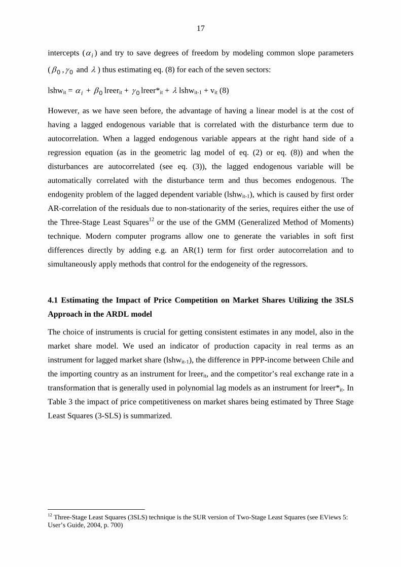
Table 3 the impact of price competitiveness on market shares being estimated by Three Stage

Least Squares (3-SLS) is summarized.

12 Three-Stage Least Squares (3SLS) technique is the SUR version of Two-Stage Least Squares (see EViews 5: User’s Guide, 2004, p. 700)

18

Table 3: Results for the ARDL market share model estimated by panel-3 SLS

Regression coefficients♣

Equation (2)

Goodness of fit measures♦

Sector-

results

Impact of

lreer

SLS03β

Impact

of lreer*

SLS03γ

Adjustm.

Coeff.

SLS3λ

AR-

term

R2adjusted S.E. of

regression

Durbin

Watson

stat.

03

short

run

0.82**

(0.02)

-0.72

(0.19)

-0.19

(0.20)

0.68***

(0.00)

0.97 1.02 2.15

08

short

run

1.82**

(0.02)

-0.14

(0.85)

-0.07

(0.70)

0.69***

(0.00)

0.99 1.05 1.99

22

short

run

-2.09***

(0.01)

2.01***

(0.01)

0.62***

(0.00)

-0.08

(0.64)

0.98 1.05 2.04

22 long

run

-6.96*** 6.04*** -------- -------- 0.98 1.05 2.04

26

short

run

1.83***

(0.00)

0.06

(0.42)

0.70***

(0.00)

-0.29*

(0.07)

0.96 1.02 2.06

26 long

run

6.10*** 0.20 --------- -------- 0.96 1.02 2.06

44

short

run

0.35

(0.76)

-2.35

(0.13)

0.46***

(0.00)

0.60***

(0.00)

0.94 1.06 2.36

♣ p-vales in brackets. ♦ In 3SLS the adjusted R2 is negative at times. It is unclear how the goodness of fit measures of the different cross-sections are to be weighted in order to derive an overall goodness of fit measure. Therefore, the figures listed should only signal the trend.

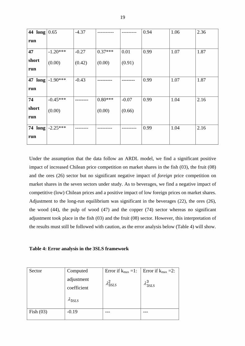
19

44 long

run

0.65 -4.37 ---------- --------- 0.94 1.06 2.36

47

short

run

-1.20***

(0.00)

-0.27

(0.42)

0.37***

(0.00)

0.01

(0.91)

0.99 1.07 1.87

47 long

run

-1.90*** -0.43 --------- -------- 0.99 1.07 1.87

74

short

run

-0.45***

(0.00)

-------- 0.80***

(0.00)

-0.07

(0.66)

0.99 1.04 2.16

74 long

run

-2.25*** -------- --------- --------- 0.99 1.04 2.16

Under the assumption that the data follow an ARDL model, we find a significant positive

impact of increased Chilean price competition on market shares in the fish (03), the fruit (08)

and the ores (26) sector but no significant negative impact of foreign price competition on

market shares in the seven sectors under study. As to beverages, we find a negative impact of

competitive (low) Chilean prices and a positive impact of low foreign prices on market shares.

Adjustment to the long-run equilibrium was significant in the beverages (22), the ores (26),

the wood (44), the pulp of wood (47) and the copper (74) sector whereas no significant

adjustment took place in the fish (03) and the fruit (08) sector. However, this interpretation of

the results must still be followed with caution, as the error analysis below (Table 4) will show.

Table 4: Error analysis in the 3SLS framework

Sector Computed

adjustment

coefficient

SLS3λ

Error if kmax =1:

23SLSλ

Error if kmax =2:

33SLSλ

Fish (03) -0.19 --- ---

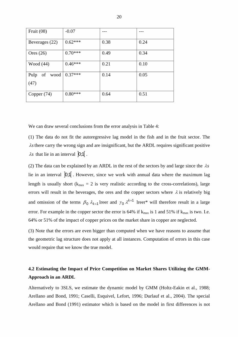
20

Fruit (08) -0.07 --- ---

Beverages (22) 0.62*** 0.38 0.24

Ores (26) 0.70*** 0.49 0.34

Wood (44) 0.46*** 0.21 0.10

Pulp of wood

(47)

0.37*** 0.14 0.05

Copper (74) 0.80*** 0.64 0.51

We can draw several conclusions from the error analysis in Table 4:

(1) The data do not fit the autoregressive lag model in the fish and in the fruit sector. The

sλ there carry the wrong sign and are insignificant, but the ARDL requires significant positive

sλ that lie in an interval . ] [10;

(2) The data can be explained by an ARDL in the rest of the sectors by and large since the sλ

lie in an interval ] [10; . However, since we work with annual data where the maximum lag

length is usually short (kmax = 2 is very realistic according to the cross-correlations), large

errors will result in the beverages, the ores and the copper sectors where λ is relatively big

and omission of the terms 0β 1+kλ lreer and 0γ1+kλ lreer* will therefore result in a large

error. For example in the copper sector the error is 64% if kmax is 1 and 51% if kmax is two. I.e.

64% or 51% of the impact of copper prices on the market share in copper are neglected.

(3) Note that the errors are even bigger than computed when we have reasons to assume that

the geometric lag structure does not apply at all instances. Computation of errors in this case

would require that we know the true model.

4.2 Estimating the Impact of Price Competition on Market Shares Utilizing the GMM-

Approach in an ARDL

Alternatively to 3SLS, we estimate the dynamic model by GMM (Holtz-Eakin et al., 1988;

Arellano and Bond, 1991; Caselli, Esquivel, Lefort, 1996; Durlauf et al., 2004). The special

Arellano and Bond (1991) estimator which is based on the model in first differences is not

21

applicable in our case since the number of instruments created by the GMM technique would

exceed the number of observations. Nonetheless, the classical GMM technique (in levels)

allows one to control for the correlation between the lagged endogenous variable and the

autocorrelated error terms. Judging from the way GMM works, this approach does have a

comparative advantage over 3SLS at controlling endogenity. Control of endogenity is 100%

due to specific model restrictions and therefore a gain in unbiasedness is obtained. However,

efficiency is lost by creating a tremendous amount of moment conditions that have to be

respected. In our case we get 210 moment conditions, i.e. 210 restrictions13, highlighting the

computational burden of this approach (Schmidt et al., 1992).

The classical GMM approach uses lagged variables as instruments for endogenous regressors.

This procedure, however, must be avoided in the presence of autocorrelation of the

distrurbances since it will not eliminate the problem of endogenity under this condition

(Durlauf et al., 2004). Therefore, we do not use lagged variables as instruments of

endogenous regressors, but the instruments of the previous section, such as the difference in

PPP-income between Chile and the importing country, an indicator of production capacity in

real terms and the real exchange rate in a transformation that is generally used in polynomial

lag models.

Table 5: Results for the ARDL market share model estimated by panel-GMM

Regression coefficients♣

Equation 2

Goodness of fit measures

Sector-

results

Impact of

lreer

GMM0β

Impact

of lreer*

GMM0γ

Adjustm.

Coeff.

GMMλ

AR-

term

R2adjusted S.E. of

regression

Durbin

Watson

stat.

03

short

run

-0.20

(0.24)

-0.78***

(0.00)

0.64***

(0.00)

-0.24**

(0.02)

0.98 1.04 2.11

03 long

run

-0.55 -2.17*** ---------- ------ 0.98 1.04 2.11

13 The number of restrictions is T(T-1) K/2. ♣ p-vales in brackets.

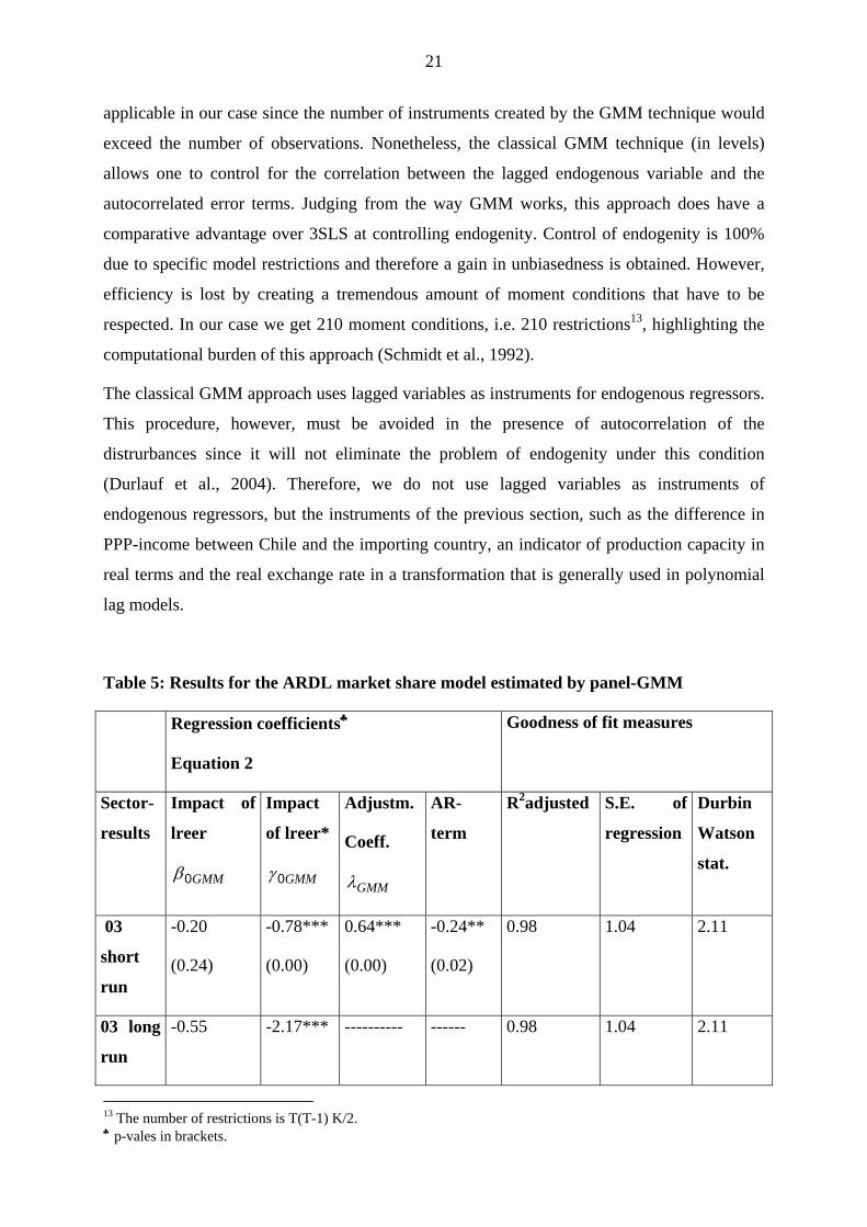
22

08

short

run

2.29*

(0.07)

-0.15

(0.90)

-0.15

(0.42)

0.69***

(0.00)

0.99 1.10 1.98

22

short

run

-2.53***

(0.00)

2.29***

(0.00)

0.58***

(0.00)

-0.13

(0.41)

0.98 1.06 2.08

22 long

run

-6.02***

5.45*** -------- -------- 0.98 1.06 2.08

26

short

run

0.32

(0.52)

-0.17

(0.13)

0.71***

(0.00)

-0.28*

(0.06)

0.89 1.04 2.04

26 long

run

1.10 0.24 ----------- --------- 0.89 1.04 2.04

44

short

run

-1.22**

(0.04)

-0.98

(0.14)

0.74***

(0.00)

-0.37***

(0.00)

0.90 1.06 2.26

44 long

run

-4.69** -3.77 ----------- --------- 0.90 1.06 2.26

47

short

run

-1.07**

(0.05)

-0.31

(0.52)

0.40***

(0.00)

-0.05

(0.80)

0.74 0.26 1.87

47 long

run

-1.78** -0.52 ----------- ---------- 0.74 0.26 1.87

74

short

run

-1.45**

(0.02)

-------- 0.37***

(0.03)

0.49***

(0.00)

0.99 1.18 2.01

74 long

run

-2.30 0.99 1.18 2.01

23

Under the assumption that the underlying assumptions of the autoregressive lag model are

fulfilled we can conclude that there is a positive relationship between an increase in Chilean

price competitiveness and market share in the fruit sector (08) and a negative relationship

between low Chilean wine prices (sector 22) and high Chilean copper prices (sector 74) and

respective market shares. Foreign relative prices have a significant impact in the fruit (03) and

beverages (22) sector. In the latter sector the quality aspect in the wine sector is supposed to

be dominant (see Table 5). The role of prices in the wood (44) and the pulp of wood (47)

sector might be severely impeded by illegal logging and illegal imports of wood products.

Illegal logging distorted official trade flows not only of all timber products (roundwood,

sawnwood, veneer, plywood, boards, semi-finished and finished products, and furniture, but

also of pulp, paper, printed products and cellulose)14. This latter statement applies also to the

interpretation of the 3SLS estimation.

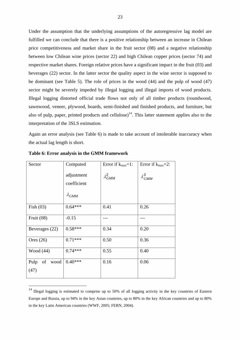
Again an error analysis (see Table 6) is made to take account of intolerable inaccuracy when

the actual lag length is short.

Table 6: Error analysis in the GMM framework

Sector Computed

adjustment

coefficient

GMMλ

Error if kmax=1:

2GMMλ

Error if kmax=2:

3GMMλ

Fish (03) 0.64*** 0.41 0.26

Fruit (08) -0.15 --- ---

Beverages (22) 0.58*** 0.34 0.20

Ores (26) 0.71*** 0.50 0.36

Wood (44) 0.74*** 0.55 0.40

Pulp of wood

(47)

0.40*** 0.16 0.06

14 Illegal logging is estimated to comprise up to 50% of all logging activity in the key countries of Eastern

Europe and Russia, up to 94% in the key Asian countries, up to 80% in the key African countries and up to 80%

in the key Latin American countries (WWF, 2005; FERN, 2004).

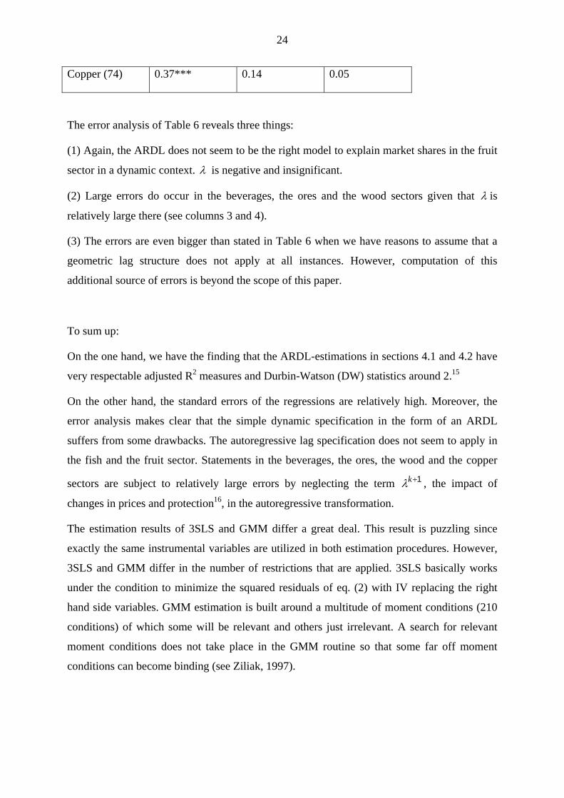
24

Copper (74) 0.37*** 0.14 0.05

The error analysis of Table 6 reveals three things:

(1) Again, the ARDL does not seem to be the right model to explain market shares in the fruit

sector in a dynamic context. λ is negative and insignificant.

(2) Large errors do occur in the beverages, the ores and the wood sectors given that λ is

relatively large there (see columns 3 and 4).

(3) The errors are even bigger than stated in Table 6 when we have reasons to assume that a

geometric lag structure does not apply at all instances. However, computation of this

additional source of errors is beyond the scope of this paper.

To sum up:

On the one hand, we have the finding that the ARDL-estimations in sections 4.1 and 4.2 have

very respectable adjusted R2 measures and Durbin-Watson (DW) statistics around 2.15

On the other hand, the standard errors of the regressions are relatively high. Moreover, the

error analysis makes clear that the simple dynamic specification in the form of an ARDL

suffers from some drawbacks. The autoregressive lag specification does not seem to apply in

the fish and the fruit sector. Statements in the beverages, the ores, the wood and the copper

sectors are subject to relatively large errors by neglecting the term , the impact of

changes in prices and protection

1+kλ16, in the autoregressive transformation.

The estimation results of 3SLS and GMM differ a great deal. This result is puzzling since

exactly the same instrumental variables are utilized in both estimation procedures. However,

3SLS and GMM differ in the number of restrictions that are applied. 3SLS basically works

under the condition to minimize the squared residuals of eq. (2) with IV replacing the right

hand side variables. GMM estimation is built around a multitude of moment conditions (210

conditions) of which some will be relevant and others just irrelevant. A search for relevant

moment conditions does not take place in the GMM routine so that some far off moment

conditions can become binding (see Ziliak, 1997).

25

5. Conclusions

Assuming that the underlying geometric lag specification can be applied to the data, the

ARDL specification allows one to draw correct inferences about the short, the medium and

the long run. The ARDL specification can be combined with the FGLS technique and is

therefore able to deal with a couple of estimation problems resulting from autocorrelation,

heteroscedasticity and cross-section correlation of the disturbances. Applied to a system of

equations, this technique transforms the variables in the regression equation through

weighting the regressor matrix with a weight matrix that can control for autocorrelation of the

disturbances, for heteroscedasticity of the variance of the residuals and for cross-section

correlation of the disturbances. The endogenity problem is solved with instrumental variables

(IV) in either a 3SLS or a GMM routine. Unlagged IV are utilized to get rid of the endogenity

problem and to obtain unbiased estimates. Furthermore, the 3SLS and the GMM- technique

are able to produce efficient and consistent estimates if ARDL is the true model.

Violation of the geometric lag assumption is to be expected in particular when working with

heterogenous panel data and with multivariate regression models. In this case a polynomial

lag model could be the model of choice if there is not excessive cross-section heterogeneity.

Estimations in the framework of panel error correction models and panel DOLS could be well

advisable, even though these models require much longer time spans to allow for meaningful

panel unit root and panel cointegration tests. Further research is needed on this topic.

15 Even though the DW must be adjusted in the presence of a lagged endogenous, the DW statistic is still able to roughly indicate problems of autocorrelation and misspecification. 16 All our prices contain sector-specific protection whenever relevant.

26

References

Ahn, S. and P. Schmidt (1995), Efficient Estimation of Models for Dynamic Panel Data,

Journal of Econometrics 68: 5-27.

Anderson, T.W. and C. Hsiao (1981), Estimation of Dynamic Models with Error

Components, Journal of the American Statistical Association; 589-606

Anderson, T.W. and C. Hsiao (1982); Formulation and Estimation of Dynamic Models Using

Panel Data, Journal of Econometrics 18: 47-82.

Arellano, M. (1989), A Note on the Anderson-Hsiao Estimator for Panel Data, Economic

Letters 31: 337-341.

Arellano, M. and S. Bond (1991), Some Tests of Specification for Panel Data: Monte Carlo

evidence and an Application to Employment Equations, Review of Economic Studies 58:

277-297.

Balestra, P. and M. Nerlove (1966), Pooling cross-section and time-series data in the

estimation of a dynamic model: The demand for natural gas, Econometrica 34: 585-612.

Baltagi, B.H. and D. Levin (1986), Estimating dynamic demand for cigarettes using panel

data: The effects of bootlegging, taxation, and advertising reconsidered, Review of

Economics and Statistics 68:148-155.Baltagi, B. H. (2005), Econometric Analysis of

Panel Data, Third Edition, Chichester […]: John Wiley & Sons, Ltd.

Blundell, R., S. Bond, M. Devereux and F. Schiantarelli (1992), Investment and Tobin’s q:

Evidence from company panel data, Journal of Econometrics 51: 233-257.

Breitung, J. and H. Pesaran (2005), Unit Roots and Cointegration in Panels,

http://www.econ.cam.ac.uk/dae/repec/cam/pdf/cwpe0535.pdf (4 November 2005).

Cable, J. R. (1997), ‘Market Share Behavior and Mobility: An Analysis and Time-series

Application, The Review of Economics and Statistics Vol. LXXIX (1): 136-141.

Durlauf, S., P. Johnson and J. Temple (2004), Growth Econometrics, social systems Research

Institute, SSRI Working Papers 18.

http://www.ssc.wisc.edu/econ/archive/wp2004-18.pdf (06 February 2006).

European Commission (2003), ‘Intra- and extra-EU trade, Annual data, Combined

Nomenclature, Supplement 2’, EUROSTAT, CD ROM of COMEXT trade data base.

EU Commission (2005),’ The EU Relations with Chile’,

http://europa.eu.int/comm/external_relations/chile/intro/ (24 November 2005)

EViews 5: User’s Guide (2004), Quantitative Micro Software, LLC, Irvine, CA.

27

FERN, Greenpeace, WWF 2004 :

http://www.panda.org/news_facts/newsroom/news.cfm?uNewsID=17214 (28 July 2005).

Greene, W. H. (2000), Econometric Analysis, London: Prentice Hall International (UK)

Limited.

Holtz-Eakin D., W. Newey and H. Rosen (1988), Estimating vector autoregressions with

panel data, Econometrica 56: 1371-1395.

Hujer, R., P. Rodrigues and C. Zeiss (2005), ‘Serial Correlation in Dynamic Panel Data

Models with Weakly Exogenous Regressors and Fixed Effects, Working Paper- March 9,

2005, J.W. Goethe-University, Frankfurt, Germany.

Im, K., M. Pesaran and Y. Shin (2003), Testing for unit roots in heterogeneous panels,

Journal of Economterics 115: 53-74.

Islam, N. (1995), Growth empirics: A panel data approach, Quarterly Journal of Economics

110, 1127-1170.

2002 Japan Conference: A Summary of the Papers, NBER Website, Friday, July 29, 2005;

http://www.nber.org/2002japanconf/sutton.html (29 July 2005).

Judson, R.. and A. Owen (1999), ‘Estimating Dynamic Panel Data Models: A Practical Guide

for Macroeconomists,’ Economic Letters 65: 9-15.

Keane, M. and D. Runkle (1992), ‘On the Estimation of Panel Data Models with Serial

Correlation when Instruments are not Strictly Exogenous,’, Journal of Business and

Economic Statistics 10(1): 1-9.

Kelejian, H.H. and W.E. Oates (1981), Introduction to Econometrics. Principles and

Applications, New York: Harper & Row Publishers.

Kim, M.K., G.D. Cho and W. W. Koo (2003), Determining Bilateral Trade Patterns Using a

Dynamic Gravity Equation, Agribusiness & Applied Economic Report No. 525, Center

for agricultural Policy and Trade Studies. North Dakota State University. http://www.ag.ndsu.nodak.edu/capts/ documents/NovemberNewsletter2003-2-4-04.pdf (3 March

2006). Kiviet, J.F. (1995), On Bias, Inconsistency, and Efficiency of Various Estimators in Dynamic

Panel Data Models, Journal of Econometrics 68: 53-78.

Koyck, L.M. (1954), Distributed Lags and Investment Analysis, Amsterdam:North Holland.

Nickell, S. (1981), Biases in Dynamic Models with Fixed Effects, Econometrica 49: 1417-

1426.

Nowak-Lehmann D., F. (2004), Different Approaches of Modeling Reaction Lags: How do

Chilean Manufacturing Exports React to Movements of the Real Exchange Rate?,

Applied Economics 36(14): 1547-1560.

28

OECD (1997), The Uruguay Round Agreement on Agriculture and Processed Agricultural

Products, OECD Publications, Paris.

Pedroni, P. (1999), Critical Values for Cointegration Tests in Heterogeneous Panels with

Multiple Regressors, Oxford Bulletin of Economics and Statistics 61 (4) Suppl.: 653-670.

Pedroni, P. (2004), Panel cointegration: asymptotic and finite sample properties of pooled

time series tests with an application to the PPP hypothesis, Econometric Theory 20: 597-

625.

Schmidt, P., S. C. Ahn and D. Wyhowski (1992), Comment, Journal of Business and

Economic Statistics 10: 10-14.

Sevestre, P. and A. Trognon (1996), ‘Dynamic Linear Models’, in The Econometrics of Panel

Data. A Handbook of the Theory with Applications, ed. By L. Mátyás and P. Sevestre, pp.

120-144, Dordrecht: Kluwer Academic Publishers, 2nd ed.

Stock, J. (1994), Unit Roots, Structural Breaks, and Trends, Chap. 46 in Handbook of

Econometrics, Vol. IV, edited by R. Engle and D. McFadden, Amsterdam: Elsevier.

Stock, J. H. and M. W. Watson (2003), Introduction to Econometrics, Boston […]: Addison

Wesley.

Sutton, J. (2004), Market share dynamics and the ‘persistence of leadership’ debate. The

Economics of Industry Group/ Suntory and Toyota International Centers for Economics

and Related Disciplines, London School of Economics, 37.

World Bank (2002), TradeCAN (Competitiveness Analysis of Nations) 2002 CD-ROM,

Washington, D.C.

World Bank (2005), World Development Indicators, Data on CD ROM, Washington, D.C.

WTO Trade Policy Review, European Union (1995, 1997, 2000), World Trade Organisation,

Geneva.

WWF (World Wildlife Fund): EU imports of wood based products 2002 (2005):

http://www.panda.org/about_wwf/where we work/europe/problems/illegal_logging/ (29

April 2005)

Ziliak, J. (1997), Efficient estimation with panel data when instruments are pretdetermined:

An empirical comparison of moment-condition estima, Journal of Business and Economic

Statistics 15: 419-431.

29

Appendix 1

Description of Data

In the following, the variables: sheu, shnoneu, shw, lreer, and lreer* will be described in

original form (not in logs). All data run from 1988 to 2002. Export data (to compute market

shares) were taken from EUROSTAT: Intra- and extra –EU trade, Supplement 2, 2003.

In our case, six cross-sections (6 EU countries: Germany, Spain, France, UK, Italy, the

Netherlands) had basically complete time series.17

(1a) Chile’s market share in the EU with respect to the EU countries: sheu

sheuist measures the share of Chilean exports (x) of sector s in EU country i at time t when

competing against imports (m) from EU countries only:

Sheuist = xist/mEUist

(1b) Chile’s market share in the EU with respect to the non-EU countries: shnoneu

shnoneuist measures the share of Chilean exports of sector s in EU country i at time t when

competing against imports (m) from non-EU countries only:

shnoneuist = xist/mnon-EUist

(1c) Chile’s market share in the EU with respect to the world (EU and non-EU

countries): shw

shwist measures the share of Chilean exports of sector s in EU country i at time t when

competing against imports (m) from EU and non-EU countries:

shwist = xist/mEU+non-EUjst

(2) The Chilean real effective exchange rate: reer

reer is the bilateral real effective exchange rate between Chile and the EU countries (price

quotation system), taking Chile’s point of view. It consists of the real exchange rate (rer) and

basic indicators of EU protection such as EU-tariffs (t) and EU-subsidies (s).

It is computed (all data for ‘rer’ are taken from World Development Indicators CD ROM of

2005) as:

rer = e ⋅ PEU/PChile with

rer = real bilateral exchange rate between Chile and relevant EU country

e = nominal exchange rate (x Chilean Peso/1EUR) between Chile and relevant EU country

PEU = GDP deflator of the EU country under consideration with 1995 as base year (1995 =̂

100)

17 Due to missing data, Austria, Belgium, Finland, Luxemburg and Sweden were excluded from the analysis.

30

PChile = GDP deflator of Chile with 1995 as base year (1995 =̂ 100)

rer has been adjusted for EU tariff protection (in terms of average EU tariff rate (t)) and non-

tariff protection (in terms of EU subsidy rate (s). Tariff rates prevailing in the EU can be

found in Trade Policy Review European Union, Volume 1, 2000, pp. 88-101 (WTO) and

rough subsidy equivalents are based on qualitative information on non-tariff protection

collected, explained and nicely put together for UNCTAD by Supper (2001).

So we get:

reer = rer ⋅ (1-s)/(1+t)

For the simulations, we assume that the FTA between Chile and the EU brings tariffs down to

zero.

(3) Chile’s competitors (*) real effective exchange rates :reer*

In analogy to (2) the real effective exchange rates of Chile’s main competitors Norway,

Australia, South Africa, Brazil are computed. Nominal exchange rates, Norway’s, Australia’s,

South Africa’s, and Brazil’s GDP deflators are computed from World Development Indicators

CD ROM 2005. Tariff and subsidy rates are borrowed from WTO and UNCTAD (see (2)).

31

Appendix 2

Figure 1: Chile’s market share in EU’s fish imports with respect to EU and non-EU

competitors in the period of 1988 to 2002

0.8

1.2

1.6

2.0

2.4

2.8

3.2

3.6

4.0

88 89 90 91 92 93 94 95 96 97 98 99 00 01 02

SHEU03 SHNONEU03 SHW03

Figure 2: Chile’s market share in EU’s fruit imports with respect to EU and non-EU

competitors in the period of 1988 to 2002

2

3

4

5

6

7

8

9

88 89 90 91 92 93 94 95 96 97 98 99 00 01 02

SHEU08 SHNONEU08 SHW08

Figure 3: Chile’s market share in EU’s imports of beverages with respect to EU and

non-EU competitors in the period of 1988 to 2002

32

0

2

4

6

8

10

12

88 89 90 91 92 93 94 95 96 97 98 99 00 01 02

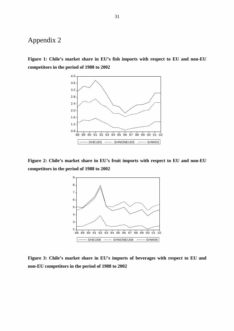
SHNONEU22 SHW22

Figure 4: Chile’s market share in EU’s imports of ores, slag and ash with respect to EU

and non-EU competitors in the period of 1988 to 2002

2

3

4

5

6

7

8

88 89 90 91 92 93 94 95 96 97 98 99 00 01 02

SHW26 SHNONEU26

Figure 5: Chile’s market share in EU’s imports of wood thereof (44) with respect to EU

and non-EU competitors in the period of 1988 to 2002

0.0

0.2

0.4

0.6

0.8

1.0

1.2

1.4

1.6

88 89 90 91 92 93 94 95 96 97 98 99 00 01 02

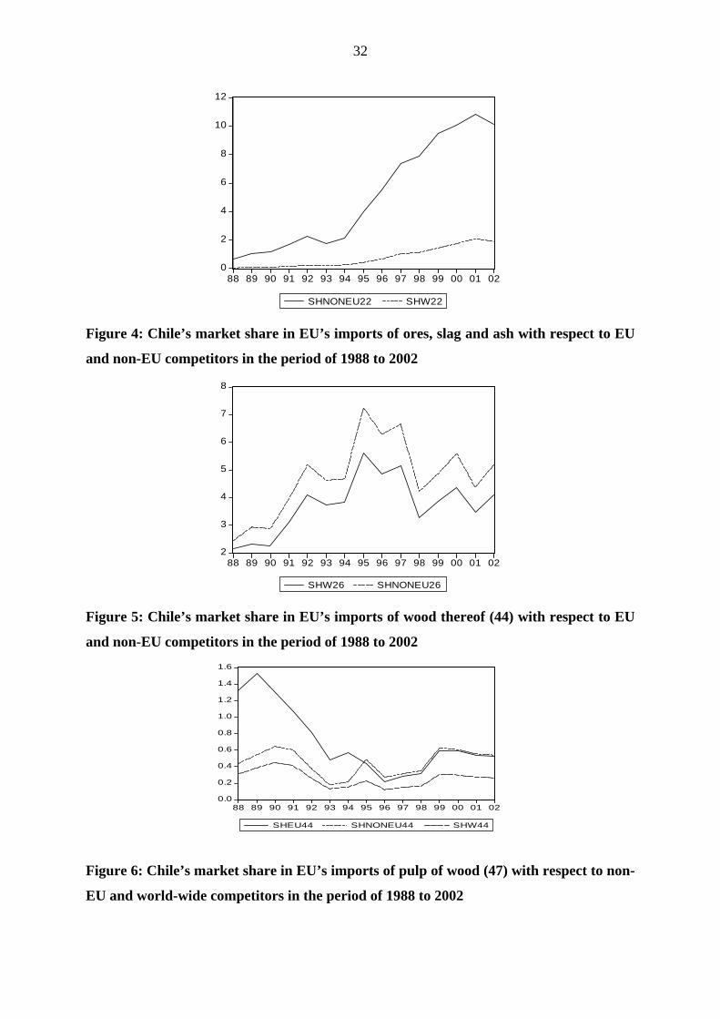
SHEU44 SHNONEU44 SHW44 Figure 6: Chile’s market share in EU’s imports of pulp of wood (47) with respect to non-

EU and world-wide competitors in the period of 1988 to 2002

33

1

2

3

4

5

6

7

8

88 89 90 91 92 93 94 95 96 97 98 99 00 01 02

SHNONEU47 SHW47

Figure 7: Chile’s market share in EU’s imports of copper (74) with respect to non-EU

and world-wide competitors in the period of 1988 to 2002

5

10

15

20

25

30

35

88 89 90 91 92 93 94 95 96 97 98 99 00 01 02

SHNONEU74 SHW74