Search  for  axions  and  ALPs    with  X-­‐ray  Polarimetry    

Enrico  Costa  IAPS  Rome  –INAF  

&  ASI  April  18-­‐19  2016,    Laboratori  Nazionali  di  Frasca=,  INFN    

The rationale

In the path from a source of X-rays to the observer and in the presence of ordered magnetic fields axion/photon coupling can introduce a linear polarization in a beam originally unpolarized or, alternatively, de-polarize an originally polarized beam (see the talk by M.Roncadelli). This suggests that X-ray Polarimetry can be a tool to search astrophysical evidences for the existence of Axions or Axion Like Particles Polarimetry is a branch of X-Ray Astronomy almost completely neglect for more than 40 years. Recently both NASA and ESA have approved advanced studies on three missions aimed to this subtopics, so that the probability that a mission of Polarimetry will fly within the next 10 years is relatively high. The most performing of the proposed mission is the X-ray Imaging Polarimetry Explorer (XIPE) one of the 3 missions candidate for ESA M4 slot. By using XIPE as a reference I try to figure how X.ray polarimetry could contribute to the quest for axions and ALP.

3  

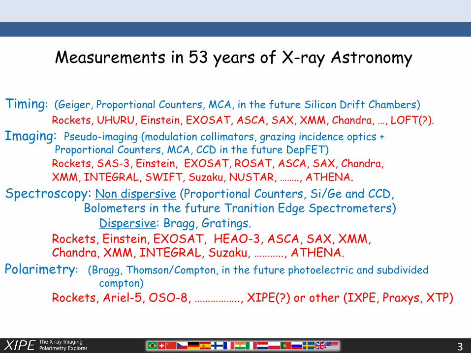
Measurements in 53 years of X-ray Astronomy

Timing: (Geiger, Proportional Counters, MCA, in the future Silicon Drift Chambers) Rockets, UHURU, Einstein, EXOSAT, ASCA, SAX, XMM, Chandra, …, LOFT(?). Imaging: Pseudo-imaging (modulation collimators, grazing incidence optics +

Proportional Counters, MCA, CCD in the future DepFET) Rockets, SAS-3, Einstein, EXOSAT, ROSAT, ASCA, SAX, Chandra, XMM, INTEGRAL, SWIFT, Suzaku, NUSTAR, …….., ATHENA.

Spectroscopy: Non dispersive (Proportional Counters, Si/Ge and CCD, Bolometers in the future Tranition Edge Spectrometers) Dispersive: Bragg, Gratings. Rockets, Einstein, EXOSAT, HEAO-3, ASCA, SAX, XMM, Chandra, XMM, INTEGRAL, Suzaku, ……….., ATHENA.

Polarimetry: (Bragg, Thomson/Compton, in the future photoelectric and subdivided compton)

Rockets, Ariel-5, OSO-8, …………….., XIPE(?) or other (IXPE, Praxys, XTP)

The status

   

  In 43 years only one positive detection of X-ray Polarization: the Crab (Novick et al. 1972, Weisskopf et al.1976, Weisskopf et al. 1978) P = 19.2 ± 1.0 %; θ = 156.4o ± 1.4o

Plus a fistful of upper limits, most of marginal significance

A vast theoretical literature, started from the very beginning of X-ry Astronomy, predicts a wealth of results from Polarimetry

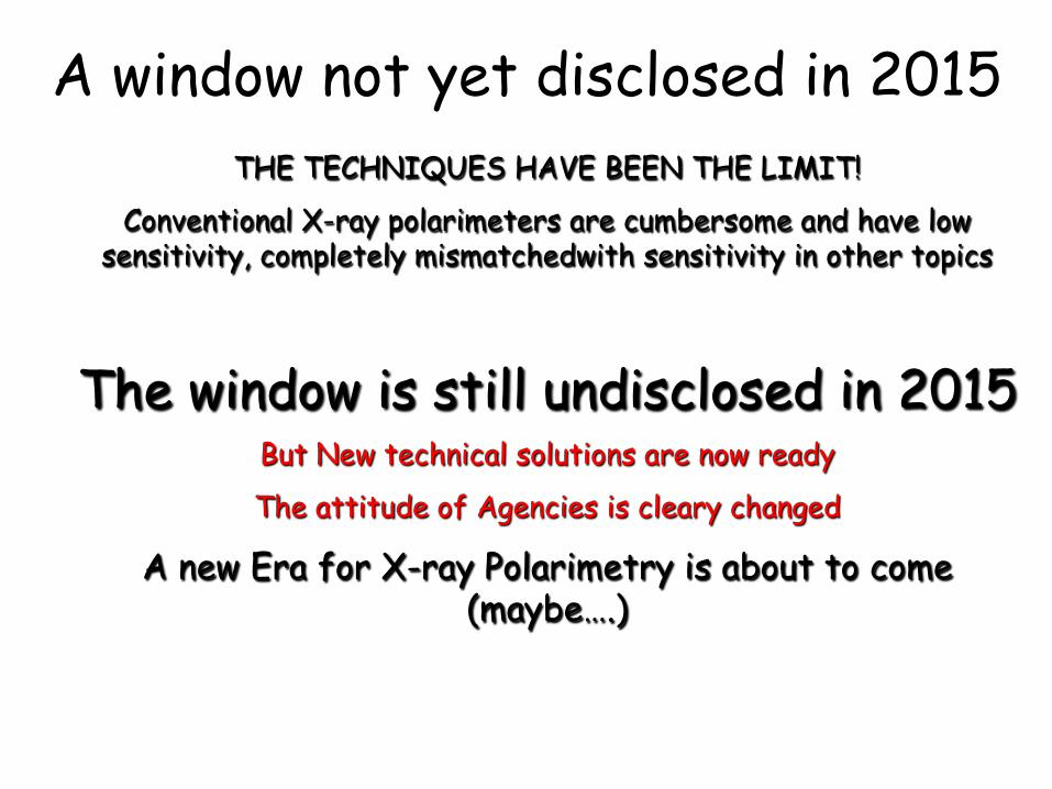
A window not yet disclosed in 2015 THE TECHNIQUES HAVE BEEN THE LIMIT!

Conventional X-ray polarimeters are cumbersome and have low sensitivity, completely mismatchedwith sensitivity in other topics

The window is still undisclosed in 2015 But New technical solutions are now ready

The attitude of Agencies is cleary changed

A new Era for X-ray Polarimetry is about to come (maybe….)

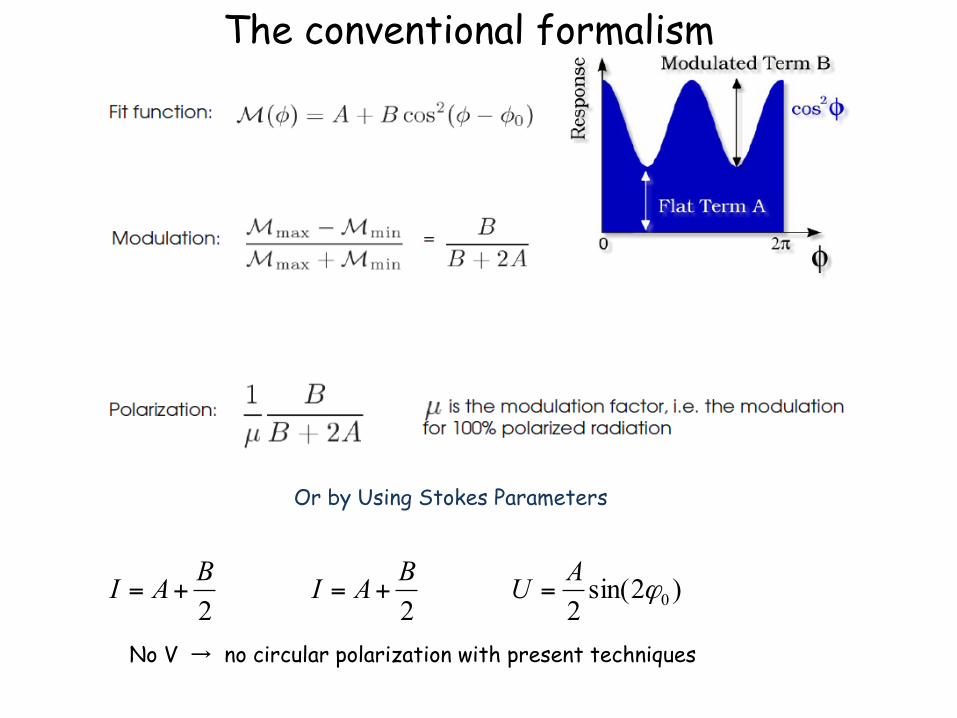
The conventional formalism

2BAI +=

2BAI += )2sin(

2 0ϕAU =

Or by Using Stokes Parameters

No V → no circular polarization with present techniques

The first limit: In polarimetry the sensitivity is a matter of photons

Source  detecAon  >  10  photons  Source  spectral  slope  >  100    photons  Source  polarizaAon  >  100.000  photons  

MDP  is  the  Minimum  Detectable  PolarizaAon  

RS  is  the  Source    rate,    RB  is  the  Background  rate,  T  is  the  observing  Ame  μ  is  the  modulaAon  factor:  the  modulaAon  of  the  response  of  the  polarimeter  to  a  100%  polarized  beam  

CauAon:  the  MDP  describes  the  capability  of  rejecAng  the  null  hypothesis  (no  polarizaAon)  at  99%  confidence.  For  a  significant  meaurement  a  longer  observaAon  is  needed.  For  a  confidence  equivalent  to  the  gaussian  5σ the constant is higher 4.29→7.58  

∂σ∂Ω

= ro2

5Z4137mc2

hν⎛

⎝ ⎜ ⎞

⎠

72 4 2 2sin θ( ) 2cos ϕ( )1 − β cos θ( )( )

4Heitler W.,The Quantum Theory of Radiation

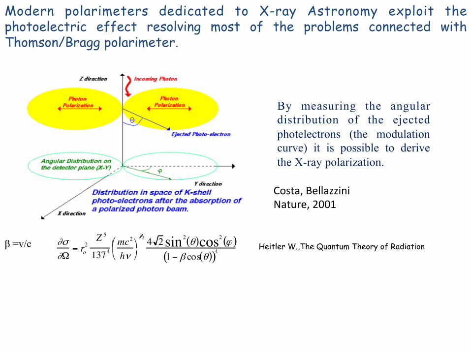
Modern polarimeters dedicated to X-ray Astronomy exploit the photoelectric effect resolving most of the problems connected with Thomson/Bragg polarimeter.

β =v/c

By measuring the angular distribution of the ejected photelectrons (the modulation curve) it is possible to derive the X-ray polarization.

Costa,  Bellazzini  Nature,  2001  

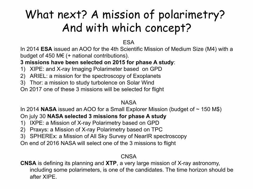
What next? A mission of polarimetry? And with which concept?

ESA In 2014 ESA issued an AOO for the 4th Scientific Mission of Medium Size (M4) with a budget of 450 M€ (+ national contributions). 3 missions have been selected on 2015 for phase A study: 1)  XIPE: and X-ray Imaging Polarimeter based on GPD 2)  ARIEL: a mission for the spectroscopy of Exoplanets 3)  Thor: a mission to study turbolence on Solar Wind On 2017 one of these 3 missions will be selected for flight

NASA In 2014 NASA issued an AOO for a Small Explorer Mission (budget of ~ 150 M$) On july 30 NASA selected 3 missions for phase A study 1)  IXPE: a Mission of X-ray Polarimetry based on GPD 2)  Praxys: a Mission of X-ray Polarimetry based on TPC 3)  SPHEREx: a Mission of All Sky Survey of NearIR spectroscopy On end of 2016 NASA will select one of the 3 missions to flight

CNSA CNSA is defining its planning and XTP, a very large mission of X-ray astronomy,

including some polarimeters, is one of the candidates. The time horizon should be after XIPE.

Let us focus on XIPE

XIPE is by far the most performing of the 3 missions under study. I use it as a reference of what X-Ray Polarimetry can do in the next future.

XIPE  parAcipaAng  InsAtuAons  BR:  INPE;  CH:  ISDC  -­‐  Univ.  of  Geneva;  CN:  IHEP,  NAOC,  NJU,  PKU,  PMO,  Purdue  Univ.,  SHAO,  Tongji  Univ,  Tsinghua  Univ.,  XAO;  CZ:  Astron.  InsAtute  of  the  CAS;  DE:   IAAT  Uni   Tübingen,  MPA,  MPE;  ES:   CSIC,   CSIC-­‐IAA,   CSIC-­‐IEEC,   CSIC-­‐INTA,  IFCA  (CSIC-­‐UC),  INTA,  Univ.  de  Valencia;  FI:  Oxford  Instruments  AnalyAcal  Oy,  Univ.  of  Helsinki,  Univ.  of  Turku;  FR:  CNRS/ARTEMIS,  IPAG-­‐Univ.  of  Grenoble/CNRS,   IRAP,   Obs.   Astron.   de   Strasbourg,   IN:   Raman   Research   InsAtute,  Bangalore;  IT:  Gran  Sasso  Science  InsAtute,  L'Aquila,  INAF/IAPS,  INAF/IASF-­‐Bo,  INAF/IASF-­‐Pa,   INAF-­‐OAA,   INAF-­‐OABr,   INAF-­‐OAR,   INFN-­‐Pi,   INFN-­‐Torino,   INFN-­‐Ts,   Univ   of   Pisa,   Univ.   Cagliari,   Univ.   of   Florence,   Univ.   of   Padova,   Univ.   of  Palermo,   Univ.   Roma   Tre,   Univ.   Torino;   NL:   JIVE,   Univ.   of   Amsterdam;  PL:CopernicusAstr.   Ctr.,   SRC-­‐PAS;  PT:   LIP/Univ.   of   Beira-­‐Interior,   LIP/Univ.   of  Coimbra;   RU:   Ioffe   InsAtute,   St.Petersburg:   SE:   KTH   Royal   InsAtute   of  Technology.  Stockholm  Univ.:  UK:  Cardiff  Univ.,  UCL-­‐MSSL,  Univ.  of  Bath;  US:  CFA,   Cornell   Univ.,   NASA-­‐MSFC,   Stony   Brook   Univ.,   Univ.   of   Iowa,   Boston  Univ.,  InsAtute  for  Astrophysical  Research,  Boston  Univ.,  Stanford  Univ./KIPAC.  

   

Proposed  by    Paolo  SoffiLa,  Ronaldo  Bellazzini,  Enrico  Bozzo,  Vadim  Burwitz,  Alberto  J.  Castro-­‐Tirado,   Enrico  Costa,   Thierry   J-­‐L.   Courvoisier,  Hua   Feng,     Szymon  Gburek,   René   Goosmann,   Vladimir   Karas,   Giorgio   MaL,   Fabio   Muleri,  Kirpal  Nandra,  Mark  Pearce,  Juri  Poutanen,  Victor  Reglero,  Maria  Dolores  Sabau,   Andrea   Santangelo,   Gianpiero   Tagliaferri,   Christoph   Tenzer,  Mar=n  C.  Weisskopf,  Silvia  Zane    

XIPE  Science  Team  Agudo,   Ivan;   Aloisio,   Roberto;   Amato,   Elena;   Antonelli,   Angelo;   Ajeia,   Jean-­‐Luc;   Axelsson,  Magnus;   Bandiera,  Rino;   Barcons,   Xavier;   Bianchi,   Stefano;   Blasi,   Pasquale;   Boër,  Michel;   Bozzo,   Enrico;   Braga,   Joao;   BuccianAni,  Niccolo';   Burderi,   Luciano;   Bykov,   Andrey;   Campana,   Sergio;   Campana,   Riccardo;   Cappi,   Massimo;   Cardillo,  MarAna;  Casella,  Piergiorgio;  Castro-­‐Tirado,  Alberto  J.;  Chen,  Yang;  Churazov,  Eugene;  Connell,  Paul;  Courvoisier,  Thierry;  Covino,  Stefano;  Cui,  Wei;  Cusumano,  Giancarlo;  Dadina,  Mauro;  De  Rosa,  Alessandra;  Del  Zanna,  Luca;  Di  Salvo,  Tiziana;  Donnarumma,   Immacolata;  Dovciak,  Michal;  Elsner,  Ronald;  Eyles,  Chris;  Fabiani,  Sergio;  Fan,  Yizhong;  Feng,  Hua;  Ghisellini,  Gabriele;  Goosmann,  René  W.;  Gou,  Lijun;  Grandi,  Paola;  Grosso,  Nicolas;  Hernanz,  Margarita;  Ho,  Luis;  Hu,  Jian;  Huovelin,  Juhani;   Iaria,  Rosario;  Jackson,  Miranda;  Ji,  Li;  Jorstad,  Svetlana;  Kaaret,  Philip;  Karas,  Vladimir;  Lai,  Dong;  Larsson,  Josefin;  Li,  Li-­‐Xin;  Li,  Tipei;  Malzac,  Julien;  Marin,  Frédéric;  Marscher,  Alan;  Massaro,  Francesco;  Maj,  Giorgio;  Mineo,  Teresa;  Miniup,  Giovanni;  Morlino,  Giovanni;  Mundell,  Carole;  Nandra,  Kirpal;  O'Dell,  Steve;  Olmi,  Barbara;  Pacciani,  Luigi;  Paul,  Biswajit;  Perna,  Rosalba;  Petrucci,  Pierre-­‐Olivier;  Pili,   Antonio  Graziano;   Porquet,   Delphine;   Poutanen,   Juri;   Ramsey,   Brian;   Razzano,  Massimiliano;   Rea,   Nanda;  Reglero,   Victor;   Rosswog,   Stephan;   Rozanska,   Agata;   Ryde,   Felix;   Sabau,  Maria  Dolores;   SalvaA,  Marco;   Silver,  Eric;  Sunyaev,  Rashid;  Tamborra,  Francesco;  Tavecchio,  Fabrizio;  Taverna,  Roberto;  Tong,  Hao;  Turolla,  Roberto;  Vink,  Jacco;  Wang,  Chen;  Weisskopf,  MarAn  C.;  Wu,  Kinwah;  Wu,  Xuefeng;  Xu,  Renxin;  Yu,  Wenfei;  Yuan,  Feng;  Zane,  Silvia;  Zdziarski,  Andrzej  A.;  Zhang,  Shuangnan;  Zhang,  Shu.    

XIPE  Instrument  Team  Baldini,  Luca;  Basso,  Stefano;  Bellazzini,  Ronaldo;  Bozzo,  Enrico;  Brez,  Alessandro;  Burwitz,  Vadim;  Costa,  Enrico;  Cui,  Wei;  de  Ruvo,  Luca;  Del  Monte,  Ejore;  Di  Cosimo,  Sergio;  Di  Persio,  Giuseppe;  Dias,  Teresa  H.  V.  T.;  Escada,  Jose;  Evangelista,  Yuri;  Eyles,  Chris;  Feng,  Hua;  Gburek,  Szymon;  Kiss,  Mózsi;  Korpela,  Seppo;  Kowaliski,  Miroslaw;  Kuss,  Michael;  Latronico,  Luca;  Li,  Hong;  Maia,  Jorge;  MinuA,  Massimo;  Muleri,  Fabio;  Nenonen,  Seppo;  Omodei,  Nicola;  Pareschi,  Giovanni;  Pearce,  Mark;  Pesce-­‐Rollins,  Melissa;  Pinchera,  Michele;  Reglero,  Victor;  Rubini,  Alda;  Sabau,   Maria   Dolores;   Santangelo,   Andrea;   Sgrò,   Carmelo;   Silva,   Rui;   Soffija,   Paolo;   Spandre,   Gloria;   Spiga,  Daniele;  Tagliaferri,  Gianpiero;  Tenzer,  Christoph;  Wang,  Zhanshan;  Winter,  Berend;  Zane,  Silvia.  

X-ray Imaging Polarimetry Explorer

12  

The  X-­‐ray  Imaging  Polarimetry  Explorer  

XIPE  is  devoted  to  observa=on  of  celes=al  sources  in  X-­‐rays    XIPE  uniqueness:  

•   Time-­‐,  spectrally-­‐,  spaAally-­‐resolved  X-­‐ray  polarimetry  as  a  breakthrough  in  high  energy  astrophysics  and  fundamental  physics    

•     It  will  explore  this  observaAonal  window  ater  40  years  from  the  last  posiAve  measurement,  with  a  dramaAc  improvement  in  sensiAvity:  from  one  to  hundred  sources  

 In  the  violent  X-­‐ray  sky,  polarimetry  is  expected  to  have  a  much  greater  impact  than  in  most  other  wavelengths.    XIPE  is  going  to  exploit  the  complete  informaAon  contained  in  X-­‐rays.    

13  

Why  this  is  now  possible  The  Gas  Pixel  Detector  

We  developed  at  this  aim  The  Gas  Pixel  Detector  a  polarizaAon-­‐sensiAve  instrument  capable  of  imaging,  Aming  and  spectroscopy  

E.  Costa,  R.Bellazzini  et  al.  2001  •  The core: an asic chip

• Peaking time: 3-10 µs, externally adjustable; •  Full-scale linear range: 30000 electrons; •  Pixel noise: 50 electrons ENC; •  Read-out mode: asynchronous or synchronous; •  Trigger mode: internal, external or self-trigger; •  Read-out clock: up to 10MHz; •  Self-trigger threshold: 2200 electrons (10% FS); •  Frame rate: up to 10 kHz in self-trigger mode (event window); •  Parallel analog output buffers: 1, 8 or 16; •  Access to pixel content: direct (single pixel) or serial (8-16 clusters, full matrix, region of interest); •  Fill fraction (ratio of metal area to active area): 92%)

A Gas Pixel Detector with: 1 Atm DME 80% He 20% 10 mm absorption/drift gap 50 µm pitch GEM Existing ASIC (100000 pixel, 50 µm pitch, auto-trigger, ROI)

14  

Why  this  is  now  possible  The  Gas  Pixel  Detector    

Image   of   a   real   photoelectron   track.   The   use   of   the   gas  allows  to  resolve  tracks  in  the  X-­‐ray  energy  band.  

Real  modulaAon  curve  derived  from  the  measurement  of  the  emission  direcAon  of  the  photoelectron.    

ModulaAon  factor  as  a  funcAon  of  energy.   Residual  modulaAon  for  unpolarised  photons.  

Bellazzini  et  al.  2012  

Muleri  et  al.  2008,2010  

STSM acknowledged in the paper by Fabiani et al.2014

Imaging  capabiliAes  of  GPD  tested  at  PANTER  

ROSAT  PSPC    

•   Good  spaAal  resoluAon:  90  µm  Half  Energy  Width  

•   Imaging  capabiliAes  on-­‐  and  off-­‐axis  measured  at  PANTER  with  a  JET-­‐X  telescope  (Fabiani  et  al.  2014)  

•   Angular  resoluAon  for  XIPE:  <26  arcsec  

16  

The  Gas  Pixel  Detector  Spectroscopic  capabili=es  

•   Adequate  spectrometer  for  conAnuum  emission  (16  %  at  6  keV,  Muleri  et  al.  2010).  

•   Stable  operaAon  over  3  years  

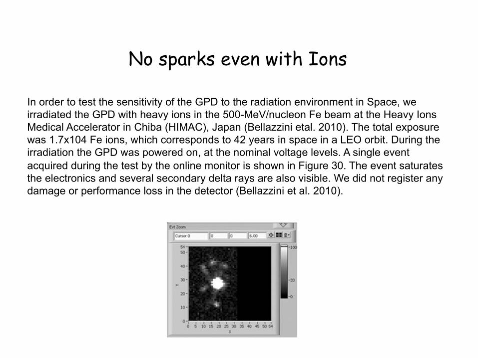
No sparks even with Ions

In order to test the sensitivity of the GPD to the radiation environment in Space, we irradiated the GPD with heavy ions in the 500-MeV/nucleon Fe beam at the Heavy Ions Medical Accelerator in Chiba (HIMAC), Japan (Bellazzini etal. 2010). The total exposure was 1.7x104 Fe ions, which corresponds to 42 years in space in a LEO orbit. During the irradiation the GPD was powered on, at the nominal voltage levels. A single event acquired during the test by the online monitor is shown in Figure 30. The event saturates the electronics and several secondary delta rays are also visible. We did not register any damage or performance loss in the detector (Bellazzini et al. 2010).

18  

XIPE  design  guidelines  A  light  and  simple  mission  

•   Three  telescopes  with  3.5  m  (possibly  4m)  focal  length  to  fit  within  the  Vega  fairing.  Long  heritage:  SAX  →  XMM  →  Swit  →  eROSITA  →  XIPE  

•   Detectors:  convenAonal  proporAonal  counter  but  with  a  revoluAonary  readout.  •   Mild  mission  requirements:  1  mm  alignment,  1  arcmin  poinAng.  •   Fixed  solar  panel.  No  deployable  structure.  No  cryogenics.  No  movable  part  except  for  the  filter  wheels.  •   Low  payload  mass:  265  kg  with  margins.  Low  power  consumpAon:  129  W  with  margins.  •   Three  years  nominal  operaAon  life.  No  consumables.  •   Low  Earth  equatorial  orbit.  

Bellazzini  et  al.  2006,  2007  

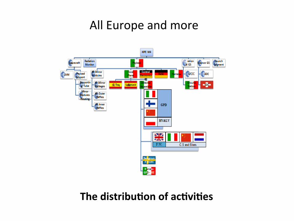
The  distribu=on  of  ac=vi=es  

 

 All  Europe  and  more        

20  

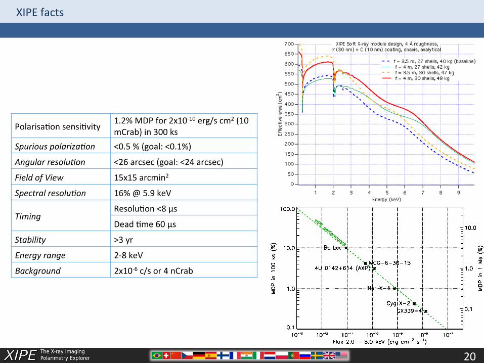
XIPE  facts  

PolarisaAon  sensiAvity  1.2%  MDP  for  2x10-­‐10  erg/s  cm2  (10  mCrab)  in  300  ks  

Spurious  polariza,on   <0.5  %  (goal:  <0.1%)    

Angular  resolu,on   <26  arcsec  (goal:  <24  arcsec)  

Field  of  View   15x15  arcmin2  

Spectral  resolu,on   16%  @  5.9  keV  

Timing  ResoluAon  <8  μs  

Dead  Ame  60  μs  

Stability   >3  yr  

Energy  range   2-­‐8  keV  

Background   2x10-­‐6  c/s  or  4  nCrab  

21  

A  world-­‐wide  open  European  observatory  

CP:  Core  Program  (25%):    

•   To  ensure  that  the  key  scienAfic  goals  are  reached  by  observing  a  set  of  representaAve  candidates  for  each  class.  

   GO:  Guest  Observer  program  on  compe==ve  base  (75%):    

•   To  complete    the  CP  with  a  fair  sample  of  sources  for  each  class;    •   To  explore  the  discovery  space  and  allow  for  new  ideas;  

•   To  engage  a  community  as  wide  as  possible.    In  organising  the  GO,  a  fair  Ame  for  each  class  will  be  assigned.  This  will  ensure  “populaAon  studies”  in  the  different  science  topics  of  X-­‐ray  polarimetry.  

   

22  

Why  do  we  need  X-­‐ray  polarimetry?  

In  X-­‐ray  sources  it  is  more  common  that  in  other  wavelengths  to  find:  •   Aspherical  emission/scajering  geometries  (disk,  blobs  and  columns,  coronae);      •   Non-­‐thermal  processes  (synchrotron,  cyclotron  and  non-­‐thermal  bremsstrahlung).  

Furthermore,  fundamental  physics  effects  like,  e.g.,  QED  birefringence  in  strong  magneAc  fields,  can  be  studied  by  X-­‐ray  polarimetry.    Timing  &  spectroscopy  may  provide  rather  ambiguous  and  model  dependent  informaAon.    What  XIPE  can  do:  

•   Resolved  sources:  Emission  mechanisms  and  mapping  of  the  magneAc  field:  PWNs,  SNR    and  extragalacAc    jet    •   Unresolved  sources:  Geometrical  parameter  of  inner  part  of  compact  sources:    X-­‐ray  pulsars,    Coronae  in  XRB  and  AGNs.    

Of  course  let  us  focus  on  unresolved    galac=c  sources    

But  is  imaging  useless  for  compact  sources?  

23  

AcceleraAon  phenomena:  The  Crab  Nebula  OSO-­‐8    measured  the  polariza=on  of  the  Crab  Neula+pulsar  as  a  whole.  But  ager  Chandra  image    ...  

Region   σdegree  (%)  

σangle  (deg)  

MDP  (%)  

1   ±0.60   ±0.96   1.90  2   ±0.41   ±0.65   1.30  3   ±0.68   ±1.10   2.17  4   ±0.86   ±1.39   2.76  5   ±0.61   ±0.97   1.93  6   ±0.46   ±0.75   1.48  7   ±0.44   ±0.70   1.40  8   ±0.44   ±0.71   1.41  9   ±0.46   ±0.74   1.47  10   ±0.60   ±0.97   1.92  11   ±0.52   ±0.83   1.65  12   ±0.53   ±0.85   1.69  13   ±0.59   ±0.95   1.89   20  ks  with  XIPE  

•  The  OSO-­‐8  observaAon,  integrated  on  the  whole  nebula,  measured  a  posiAon  angle  which  is  Alted  with  respect  to  jets  and  torus  axes.  It  was  not  possible  to  measure  the  polarizaAon    of  PSR0531+21  because  the  contribuAon  to  the  total  counts  was  around  4%  and  the  nebula  was  acAng  as  a  huge  background.  

     •  XIPE  has  a  resoluAon  which  is  not  imaging  capabiliAes  will  allow  to  measure  the  pulsar  polarisaAon  

by  separaAng  from  the  much  brighter  nebula  emission.  

XIPE  scien=fic  goals Astrophysics:  Accelera=on:  SNR  

Map  of  the  magne-c  field Spectral  imaging  allows  to  separate  the  thermalised  plasma  from  the  regions  where  shocks  accelerate  parAcles.   What  is  the  orientaAon  of  the  magneAc  field?  How  ordered  is  it?  The  spectrum  cannot  tell…

2  Ms  observaAon  with  XIPE 4-­‐6  keV  image  of  Cas  A  blurred  with  the  PSF  of  XIPE

XIPE  scien=fic  goals Astrophysics:  Accelera=on:  Unresolved  Jets  in  Blazars  

                        SchemaAc   view   of   an   AGN ➡ Blazars  are  those  AGN  which  not  only  have  a  jet   (like   all   radiogalaxies),   but   it   is   directed  towards  us. Due  to  a  Special  RelaAvity  effect  (aberraAon),  the   jet   emission   dominates   over   other  emission  components  

XIPE  scien=fic  goals Astrophysics:  Strong  Magne=c  Fields:  Accre=ng    Millisecond    Pulsars

Viironen  &  Poutanen  2004

Emission  due  to  scajering  in  hot  spots   ⇒   Phase-­‐dependent  linear  polarizaAon    

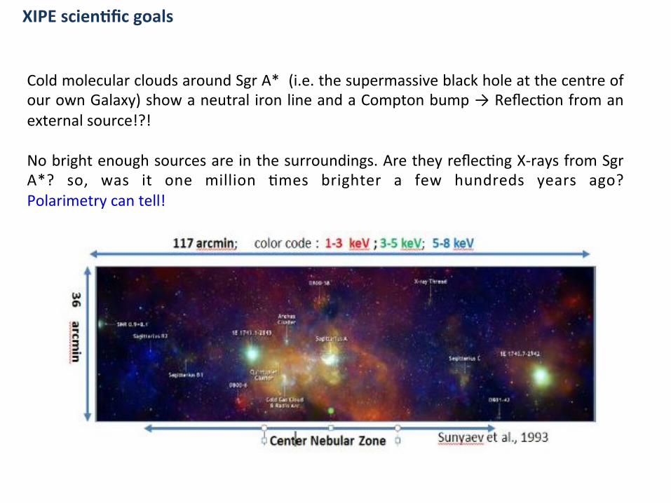
XIPE  scien=fic  goals Astrophysics:  ScaLering:  X-­‐ray  reflec=on  nebulae  in  the  GC

Cold  molecular  clouds  around  Sgr  A*    (i.e.  the  supermassive  black  hole  at  the  centre  of  our  own  Galaxy)  show  a  neutral   iron  line  and  a  Compton  bump  →  ReflecAon  from  an  external  source!?! No  bright  enough  sources  are  in  the  surroundings.  Are  they  reflecAng  X-­‐rays  from  Sgr  A*?   so,   was   it   one   million   Ames   brighter   a   few   hundreds   years   ago?                                          Polarimetry  can  tell!

XIPE  scien=fic  goals Astrophysics:  ScaLering:  X-­‐ray  reflec=on  nebulae  in  the  GC

Polariza=on  by  scaLering  from  Sgr  B  complex,  Sgr  C  complex •       The  angle  of  polarisaAon  pinpoints  the  source  of  X-­‐rays   •       The  degree  of  polarizaAon  measures  the  scajering  angle  and                                            determines  the  true  distance  of  the  clouds  from  Sgr  A*.  

Marin  et  al.  2014

29  

Emission  in  strong  magneAc  field:  X-­‐ray  pulsars  Disentangling  geometric  parameters    from  physical  ones    

9 keV

3.8 keV

1.6 keV

9 keV

3.8 keV

1.6 keV

9 keV 3.8 keV

1.6 keV

Accreting X-ray PulsarX-ray emission from a binary pulsar will be polarized by:

•Emission process: cyclotron•Scattering on aspherical (column) accreting plasma• Scattering on highly magnetized plasma: σ║≠ σ┴• Vacuum polarization and birefringence through extreme magnetic fields

The swing of the polarization angle with phase directly measure the orientation of the rotation axis on the sky and the inclination of the magnetic field: in the figure the case 45°, 45°(from Meszaros et al. 1988)

Emission  process:  •   cyclotron  •   opacity  on  highly  magneAsed  plasma: k┴ < k║ From  the  swing  of  the  polarisaAon  angle:  •   OrientaAon  of  the  rotaAon  axis      •   InclinaAon  of  the  magneAc  field  •   Geometry  of  the  accreAon  column:  “fan”  beam  vs  “pencil”  beam    

Meszaros  e

t  al.  1988  

For the best class of XIPE candidates we use a paper 27 y old!

30  

Birefringence  in  the  magnetosphere  of  magnetars  More  papers  on    isolated  neutron  stars  

A  twisted  magneAc  field.  Magnetars  are  isolated  neutron  stars  with  likely  a  huge  magneAc  field  (B  up  to  1015  Gauss).    It  heats  the  star  crust  and  explains  why  the  X-­‐ray  luminosity  largely  exceeds  the  spin  down  energy  loss.    QED  foresees  vacuum  birefringence,  an  effect  predicted  80  years  ago,  expected  in  such  a  strong  magneAc  field  and  never  detected  yet.  

Such  an  effect  is  only  visible  in  the  phase  dependent  polarizaAon  degree  and  angle.  

Light  curve   Polarisa=on  degree   Polarisa=on  angle  

31  

Disentangling  the  geometry  of  the  hot  corona  in  AGN  and  X-­‐ray  binaries  Constraining  components  of  X-­‐ray  emission  from  AGNs  

The  geometry  of  the  hot  corona  of  electrons,  considered  to  be  responsible  for  the  (non-­‐disc)  X-­‐ray  emission  in  binaries  and  AGN,  is  largely  unconstrained.  

The  geometry  is  related  to  the  corona  origin:  •   Slab  –  high  polarisaAon  (up  to  more  than  10%):  disc  instabiliAes?  •   Sphere  –  very  low  polarisaAon:  aborted  jet?  

 The  sensiAvity  of  XIPE  will  allow  to  detect  the  polarisaAon  of  the  corona  in  a  large  sample  of  binaries  and  AGN.    

SLAB  

SPHERE  

Marin  &  Tamborra  2014  

Even  larger  (more  than  20%)  polarisaAon  is  expected  if  the  X-­‐ray  emission  of  galacAc  black  hole  candidates  in  hard  states  is  due  to  jet.  

32  

Constraining  black  hole  spin  with  XIPE  An  overdetermined  problem:  let  us  increase  the  confusion  

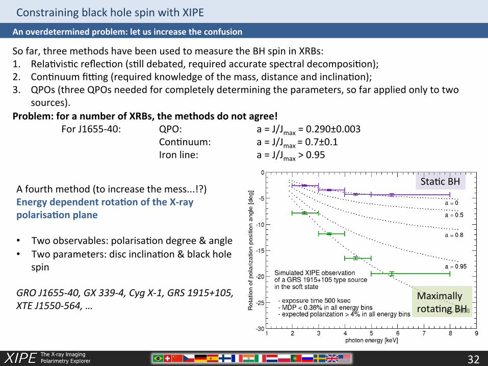
So  far,  three  methods  have  been  used  to  measure  the  BH  spin  in  XRBs:  1.  RelaAvisAc  reflecAon  (sAll  debated,  required  accurate  spectral  decomposiAon);  2.  ConAnuum  fipng  (required  knowledge  of  the  mass,  distance  and  inclinaAon);  3.  QPOs  (three  QPOs  needed  for  completely  determining  the  parameters,  so  far  applied  only  to  two  

sources).  Problem:  for  a  number  of  XRBs,  the  methods  do  not  agree!  

 For  J1655-­‐40:  QPO:    a  =  J/Jmax  =  0.290±0.003        ConAnuum:  a  =  J/Jmax  =  0.7±0.1        Iron  line:    a  =  J/Jmax  >  0.95  

A  fourth  method  (to  increase  the  mess...!?)  Energy  dependent  rota=on  of  the  X-­‐ray  polarisa=on  plane    •  Two  observables:  polarisaAon  degree  &  angle  •  Two  parameters:  disc  inclinaAon  &  black  hole  

spin    GRO  J1655-­‐40,  GX  339-­‐4,  Cyg  X-­‐1,  GRS  1915+105,  XTE  J1550-­‐564,  …  

StaAc  BH  

Maximally    rotaAng  BH  

33  

Many  sources  in  each  class  available  for  XIPE  

100  –  150  quoted  in  the  proposal:  •   500  days  of  net  exposure  Ame  in  3  years;  •   average  observing  Ame  of  3  days;  •   re-­‐visiAng  for  some  of  those.      

   What  number  for  each  class?  

Target  Class Ttot  (days)

Tobs/source  (Ms)

MDP    (%)

Number  in  3  years

Number  available

AGN 219 0.3 <  5 73 127 XRBs    

(low+high  mass) 91 0.1 <  3 91 160

SNRe 80 1.0 <  15  %  (10  regions) 8 8 PWN 30 0.5 <10  %  (more  than  5  regions) 6 6

Magnetars 50 0.5 <  10  %  (in  more  than  5  bins) 10 10 Molecular  clouds

30 1-­‐2 <  10  % 2  complexes  or  5  

clouds 2  complexes  or  5  clouds

Total 500     193 316

From  catalogues:  Liu  et  al.  2006,  2007  for  X-­‐ray  binaries;  and  XMM  slew  survey  1.6  for  AGNs.  

Summary

XIPE  will  open  a  new  observa=onal  window,  adding  the  two  missing  observables  in  X-­‐rays. Many  X-­‐ray  sources  are  aspherical  and/or  non-­‐thermal  emiLers,  so  radia=on  must  be  highly  polarised. XIPE  is  simple  and  ready,  using  pioneering,  yet  mature,  technology.    Coverage  of  theore=cal  work  on  different  topics  is    unevenly  covered.  This  is  natural,  given  the  absence  of  data.  But  to  plan  the  observa=ons  is  not  very  good.    Predic=ons  on  some  of  the  most  straighrorward  targets  for  XIPE,  such  as  bright  binares    with  NS  are  based  on  a  few  old  papers.        

Let us try to single out topics that we can figure could provide astrophysical evidences for ALPs.

What has X-Ray Polarimetry to do with ALPs?

γALP oscillation can only occurr in presence of an external Magnetic Field. Only photons γǁ‖ with polarization parallel to the plane defined from the direction and B mix. If the magnetic field is oriented the oscllation changes the polarization properties of the beam. The effect should be visible on long distance scale if we assume magnetic fields in intercluster space are ordered within domains of few Mpcs.

Axions and ALP have two ways to show up through polarization

If the assumption is correct we should detect effects that increase with the distance of the source. . 1) By introducing an unexpected polarization on sources that we have good reasons to assume to be unpolarized in thir frame 2) By decreasing polarization amount and changing polarization angle in the flux of sources for which we can make a reasonable assumption on whic was the polarization in their frame. Both cases have been discussed by Nicola Bassan, Alessandro Mirizzi and Marco Roncadelli, Journal of Cosmology and Astroparticle Physics, Volume 2010, May 2010and applied to GRBs. I try to extend the computations to steady sources.

A totally umpolarized source: the cluster of galaxies Galaxy clusters have a well studied thermal spectrum with a bremsstrahlung continuum and lines, possibly with different components (temperatures). NUSTAR observations do not confirm the presence of a non-thermal component of Inverse Compton, suggested in the past for a few objects. we can assume that a cluster should be polarized ~0% (≤ 0.2% Komarov et al. Submitted) . With XIPE we can detect possible polarization from a rich sample of clusters.

HEAO1A2  (Piccinos  et  al.1982)  

Name   Flux  (2-­‐10eV)  10-­‐11  erg  cm-­‐2s-­‐1  

Z   D  (Mpc)   MDP  For  105  s  

H0039-­‐0396   Abell  85   6.6   0.0499   212.6   3.9  H0054-­‐015   Abell  119   4.4   0.0446   190.3   4.8  H0256+134   Abell  401   7.3   0.0748   316.9   3.7  H0335+096   0335+096   3.2   0.04   170.8   5.6  H0411+104   Abell  478   6.5   0.09   382.2   3.9  H0431-­‐134   Abell  496   5.4   0.036   154.2   4.3  H1347+268   Abell  1795   5.9   0.0621   263.9   4.1  H1556+274   Abell  2142   7.6   0.0903   381.3   3.6  H1600+171   Abell  2147   5.0   0.0377   161.1   4.5  H1627+396   Abell  2199   7.5   0.0312   133.5   3.7  

If we detect a polarization and if it increases in average with the distance we can work on the hypothesis that ALP photon coupling is producinging it. Of course we should disentingle the effects of the same process in our galaxy and within the cluster itself but this is not impossible because the magnetic fields are known.

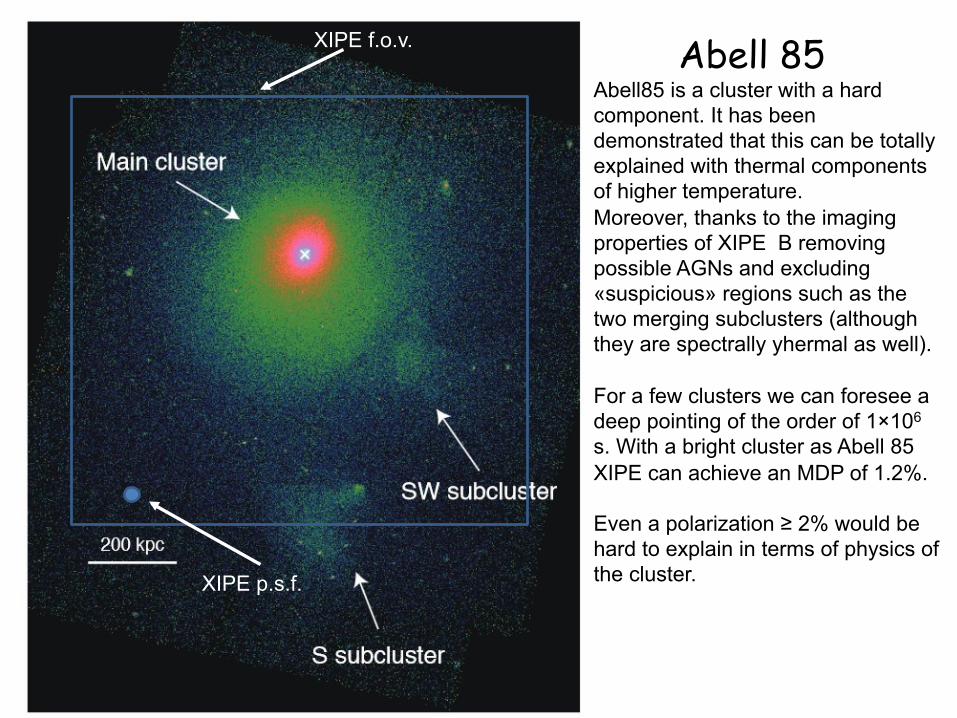
Abell 85 XIPE f.o.v.

Abell85 is a cluster with a hard component. It has been demonstrated that this can be totally explained with thermal components of higher temperature. Moreover, thanks to the imaging properties of XIPE B removing possible AGNs and excluding «suspicious» regions such as the two merging subclusters (although they are spectrally yhermal as well). For a few clusters we can foresee a deep pointing of the order of 1×106 s. With a bright cluster as Abell 85 XIPE can achieve an MDP of 1.2%. Even a polarization ≥ 2% would be hard to explain in terms of physics of the cluster.

XIPE p.s.f.

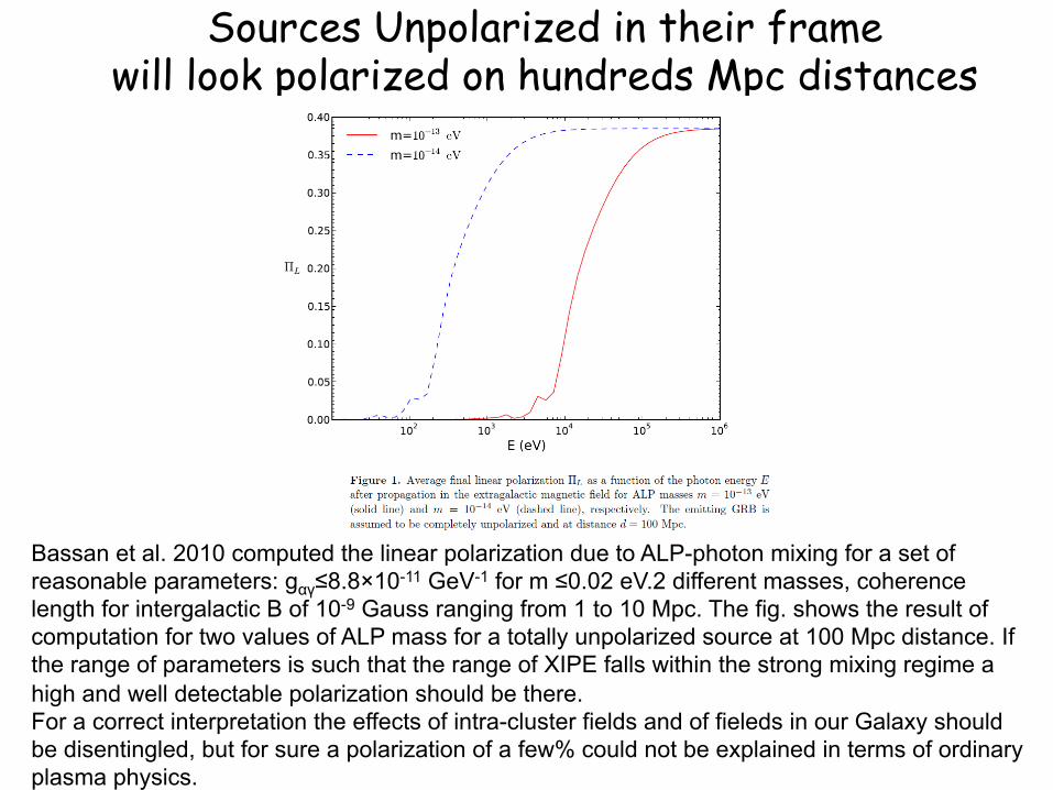
Sources Unpolarized in their frame will look polarized on hundreds Mpc distances

Bassan et al. 2010 computed the linear polarization due to ALP-photon mixing for a set of reasonable parameters: gαγ≤8.8×10-11 GeV-1 for m ≤0.02 eV.2 different masses, coherence length for intergalactic B of 10-9 Gauss ranging from 1 to 10 Mpc. The fig. shows the result of computation for two values of ALP mass for a totally unpolarized source at 100 Mpc distance. If the range of parameters is such that the range of XIPE falls within the strong mixing regime a high and well detectable polarization should be there. For a correct interpretation the effects of intra-cluster fields and of fieleds in our Galaxy should be disentingled, but for sure a polarization of a few% could not be explained in terms of ordinary plasma physics.

Astrophysics:  Accelera=on:  Unresolved  Jets  in  Blazars  

Blazars  are  extreme  accelerators  in  the  Universe,  but  the  emission  mechanism  is  far  from  being  understood. In  inverse  Compton  dominated  Blazars,  a  XIPE  observaAon  can  determine  the  origin  of  the  seed  photons: •   Synchrotron-­‐Self  Compton  (SSC)  ? The  polarizaAon  angle  is  the  same  as  for  the  synchrotron  peak. •   External  Compton  (EC)  ? The  polarizaAon  angle  may  be  different.   The   polarizaAon   degree   determines   the  electron  temperature  in  the  jet.

XIPE  band XIPE  band XIPE  band XIPE  band XIPE  band

The  other  case:  sources  where  polariza=on  is  expected

Sync.  Peak IC  Peak

More  on  blazars Astrophysics:  Accelera=on:  Unresolved  Jets  in  Blazars  

Sync.  Peak IC  Peak Sync.  Peak IC  Peak

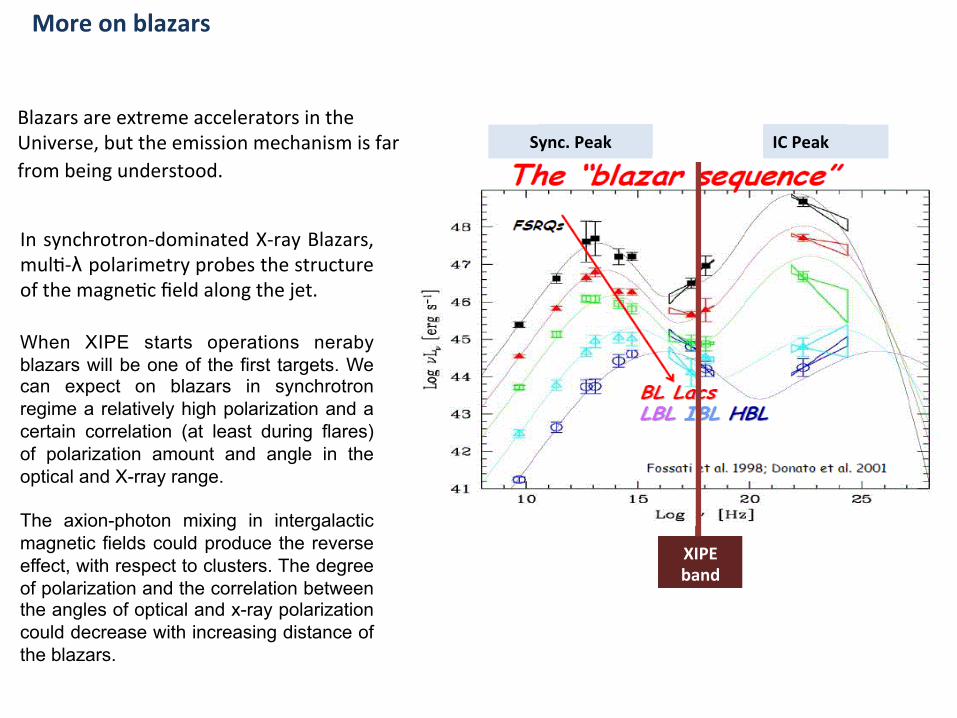
XIPE  band

In  synchrotron-­‐dominated  X-­‐ray  Blazars,  mulA-­‐λ polarimetry  probes  the  structure  of  the  magneAc  field  along  the  jet. When XIPE starts operations neraby blazars will be one of the first targets. We can expect on blazars in synchrotron regime a relatively high polarization and a certain correlation (at least during flares) of polarization amount and angle in the optical and X-rray range. The axion-photon mixing in intergalactic magnetic fields could produce the reverse effect, with respect to clusters. The degree of polarization and the correlation between the angles of optical and x-ray polarization could decrease with increasing distance of the blazars.

Sync.  Peak IC  Peak Sync.  Peak IC  Peak

XIPE  band

Sync.  Peak IC  Peak

XIPE  band

Sync.  Peak IC  Peak Sync.  Peak IC  Peak

XIPE  band

Sync.  Peak IC  Peak

XIPE  band

Sync.  Peak IC  Peak Blazars  are  extreme  accelerators  in  the  Universe,  but  the  emission  mechanism  is  far  from  being  understood.

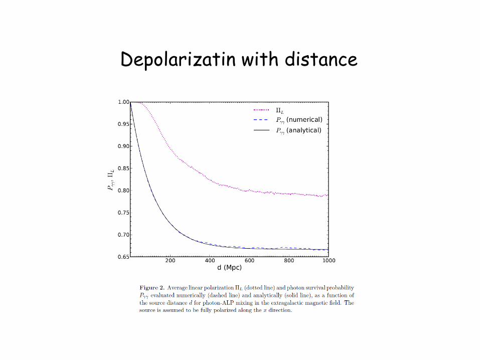
Depolarizatin with distance

Less Straightforward Observation

We know almost nothing on X-ay polarization. X-ray polarimetry is an almost totally new topics. From the first study of Blazars we should verify which is the polarimetric behavior of these objects. E.g. in flares when Optical/IR/and X radiation vary together we could expect a high polarization degree in the different bands. The effect of the ALP – axion coupling should be apparent in X-rays only. Therefore we could expect that the polarization degree in X-rays decreases with the distance in X-rays, while we already know that it does not in IR/O. Also the difference between the polarization angle in X-ray and in IR/O should increase with the distance. Likely the measurement on the angle would be more robust. With the known Blazar 1ES1101+232, at z=0.186 we can detect variations of the angle don to 2°.

44  

More  about  XIPE  

http://www.isdc.unige.ch/xipe/

The site also includes sciece working groups just set up The site includes a (very preliminary) calculater of sensitivity of XIPE for a given source and for a given observing time

Any contribution for IAXO?

Beside the scientific complementarity, the experience on the detector (performance, stability and background reduction) could contribute to IAXO design.