IAML: Support Vector Machines, Part II

IAML: Support Vector Machines, Part II

Nigel Goddard and Victor LavrenkoSchool of Informatics

Semester 1

1 / 25

Last Time

I Max margin trickI Geometry of the margin and how to compute itI Finding the max margin hyperplane using a constrained

optimization problemI Max margin = Min norm

2 / 25

This Time

I Non separable dataI The kernel trick

3 / 25

The SVM optimization problem

I Last time: the max margin weights can be computed bysolving a constrained optimization problem

minw||w||2

s.t. yi(w>xi + w0) ≥ +1 for all i

I Many algorithms have been proposed to solve this. One ofthe earliest efficient algorithms is called SMO [Platt, 1998].This is outside the scope of the course, but it does explainthe name of the SVM method in Weka.

4 / 25

Finding the optimum

I If you go through some advanced maths (Lagrangemultipliers, etc.), it turns out that you can show somethingremarkable. Optimal parameters look like

w =∑

i

αiyixi

I Furthermore, solution is sparse. Optimal hyperplane isdetermined by just a few examples: call these supportvectors

5 / 25

Why a solution of this form?

If you move the points not on the marginal hyperplanes,solution doesn’t change - therefore those points don’t matter.

~

xx

xxoo

oo

omarginw

5 / 18

6 / 25

Finding the optimum

I If you go through some advanced maths (Lagrangemultipliers, etc.), it turns out that you can show somethingremarkable. Optimal parameters look like

w =∑

i

αiyixi

I Furthermore, solution is sparse. Optimal hyperplane isdetermined by just a few examples: call these supportvectors

I αi = 0 for non-support patternsI Optimization problem to find αi has no local minima (like

logistic regression)I Prediction on new data point x

f (x) = sign((w>x) + w0)

= sign(n∑

i=1

αiyi(x>i x) + w0)

7 / 25

Non-separable training sets

I If data set is not linearly separable, the optimizationproblem that we have given has no solution.

minw||w||2


I Why?

I Solution: Don’t require that we classify all points correctly.Allow the algorithm to choose to ignore some of the points.

I This is obviously dangerous (why not ignore all of them?)so we need to give it a penalty for doing so.

8 / 25

Non-separable training sets

I If data set is not linearly separable, the optimizationproblem that we have given has no solution.

minw||w||2


I Why?I Solution: Don’t require that we classify all points correctly.

Allow the algorithm to choose to ignore some of the points.I This is obviously dangerous (why not ignore all of them?)

so we need to give it a penalty for doing so.

9 / 25

~

xx

xxoo

oo

omargin

o!

w

9 / 18

10 / 25

Slack

I Solution: Add a “slack” variable ξi ≥ 0 for each trainingexample.

I If the slack variable is high, we get to relax the constraint,but we pay a price

I New optimization problem is to minimize

||w||2 + C(n∑

i=1

ξi)k

subject to the constraints

w>xi + w0 ≥ 1− ξi for yi = +1

w>xi + w0 ≤ −1 + ξi for yi = −1

I Usually set k = 1. What if not? C is a trade-off parameter.Large C gives a large penalty to errors.

I Solution has same form, but support vectors also includeall where ξi 6= 0. Why? 11 / 25

Think about ridge regression again

I Our max margin + slack optimization problem is tominimize:

||w||2 + C(n∑

i=1

ξi)k

subject to the constraints

w>xi + w0 ≥ 1− ξi for yi = +1

w>xi + w0 ≤ −1 + ξi for yi = −1

I This looks a even more like ridge regression than thenon-slack problem:

I C(∑n

i=1 ξi)k measures how well we fit the data

I ||w||2 penalizes weight vectors with a large normI So C can be viewed as a regularization parameters, like λ

in ridge regression or regularized logistic regressionI You’re allowed to make this tradeoff even when the data

set is separable!12 / 25

Why you might want slack in a separable data set

x x

x

x

xx

x

x

oo

o

oo

oo

oo

o

o

x1

x2

wx x

x

x

xx

x

x

oo

o

oo

oo

oo

o

o

x1

x2

w

ξ

13 / 25

Non-linear SVMs

I SVMs can be made nonlinear just like any other linearalgorithm we’ve seen (i.e., using a basis expansion)

I But in an SVM, the basis expansion is implemented in avery special way, using something called a kernel

I The reason for this is that kernels can be faster to computewith if the expanded feature space is very high dimensional(even infinite)!

I This is a fairly advanced topic mathematically, so we willjust go through a high-level version

14 / 25

Kernel

I A kernel is in some sense an alternate “API” for specifyingto the classifier what your expanded feature space is.

I Up to now, we have always given the classifier a new set oftraining vectors φ(xi) for all i , e.g., just as a list of numbers.φ : Rd → RD

I If D is large, this will be expensive; if D is infinite, this willbe impossible

15 / 25

Non-linear SVMs

I Transform x to φ(x)

I Linear algorithm depends only on x>xi . Hencetransformed algorithm depends only on φ(x)>φ(xi)

I Use a kernel function k(xi ,xj) such that

k(xi ,xj) = φ(xi)>φ(xj)

I (This is called the “kernel trick”, and can be used with awide variety of learning algorithms, not just max margin.)

16 / 25

Example of kernel

I Example 1: for 2-d input space

φ(x) =

x21√

2x1x2x2

2

then

k(xi ,xj) = (x>i xj)2

17 / 25

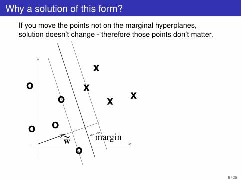
Kernels, dot products, and distance

I The Euclidean distance squared between two vectors canbe computed using dot products

d(x1,x2) = (x1 − x2)T (x1 − x2)

= xT1 x1 − 2xT

1 x2 + xT2 x2

I Using a linear kernel k(x1,x2) = xT1 x2 we can rewrite this

asd(x1,x2) = k(x1,x1)− 2k(x1,x2) + k(x2,x2)

I Any kernel gives you an associated distance measure thisway. Think of a kernel as an indirect way of specifyingdistances.

18 / 25

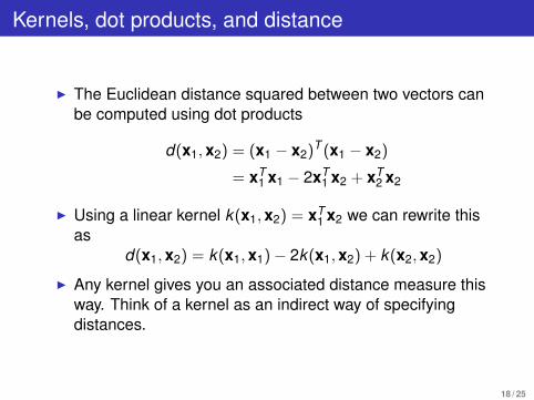
Support Vector Machine

I A support vector machine is a kernelized maximummargin classifier.

I For max margin remember that we had the magic property

w =∑

i

αiyixi

I This means we would predict the label of a test example xas

y = sign[wT x + w0] = sign[∑

i

αiyixTi x]

I Kernelizing this we get

y = sign[∑

i

αiyik(xi ,bx)]

19 / 25

Prediction on new exampleApplications

! f(x)= sgn ( + b)

input vector x

support vectors x 1 ... x 4

comparison: k(x,x i), e.g.

classification

weights

k(x,x i)=exp(!||x!x i||2 / c)

k(x,x i)=tanh("(x.x i)+#)

k(x,x i)=(x.x i)d

f(x)= sgn ( ! $i.k(x,x i) + b)

$1 $2 $3 $4

k k k k

Figure Credit: Bernhard Schoelkopf

13 / 18

� US Postal Service digit data (7291 examples, 16× 16images). Three SVMs using polynomial, RBF andMLP-type kernels were used (see Scholkopf and Smola,Learning with Kernels, 2002 for details)

� Use almost the same (� 90%) small sets (4% of database) of SVs

� All systems perform well (� 4% error)� Many other applications, e.g.

� Text categorization� Face detection� DNA analysis

14 / 18

Support Vector Regression

� The support vector algorithm can also be used forregression problems

� Instead of using squared-error, the algorithm uses the�-insensitive error

E�(z) =

� |z|− � if |z| ≥ �,0 otherwise.

� Again a sparse solution is obtained from a QP problem

f (x) =n�

i=1

βi k(x, xi) + w0

15 / 18

x

x

x x

x

xxx

x

xx

x

x

x

+!"!

x

#+!

"!0

#


The data points within the �-insensitive region have βi = 0

16 / 18


20 / 25

feature spaceinput space

!

!

!!

!"

""

""

"


� Example 2

k(xi , xj) = exp−||xi − xj ||2/α2

In this case the dimension of φ is infinite� To test a new input x

f (x) = sgn(n�

i=1

αi yik(xi , x) + w0)

11 / 18


I Example 2

k(xi ,xj) = exp−||xi − xj ||2/α2

In this case the dimension of φ is infinite. i.e., It can beshown that no φ that maps into a finite-dimensional spacewill give you this kernel.

I We can never calculate φ(x), but the algorithm only needsus to calculate k for different pairs of points.

21 / 25

Choosing φ, C

I There are theoretical results, but we will not cover them. (Ifyou want to look them up, there are actually upper boundson the generalization error: look for VC-dimension andstructural risk minimization.)

I However, in practice cross-validation methods arecommonly used

22 / 25

Example application

I US Postal Service digit data (7291 examples, 16× 16images). Three SVMs using polynomial, RBF andMLP-type kernels were used (see Scholkopf and Smola,Learning with Kernels, 2002 for details)

I Use almost the same (' 90%) small sets (4% of database) of SVs

I All systems perform well (' 4% error)I Many other applications, e.g.

I Text categorizationI Face detectionI DNA analysis

23 / 25

Comparison with linear and logistic regression

I Underlying basic idea of linear prediction is the same, buterror functions differ

I Logistic regression (non-sparse) vs SVM (“hinge loss”,sparse solution)

I Linear regression (squared error) vs ε-insensitive errorI Linear regression and logistic regression can be

“kernelized” too

24 / 25

SVM summary

I SVMs are the combination of max-margin and the kerneltrick

I Learn linear decision boundaries (like logistic regression,perceptrons)

I Pick hyperplane that maximizes marginI Use slack variables to deal with non-separable dataI Optimal hyperplane can be written in terms of support

patternsI Transform to higher-dimensional space using kernel

functionsI Good empirical results on many problemsI Appears to avoid overfitting in high dimensional spaces (cf

regularization)I Sorry for all the maths!

25 / 25

Documents

IAML: Support Vector Machines, Part II