IAEAInternational Atomic Energy Agency

Applied Statistics for Biological Dosimetry

Part 2

LectureModule 8

IAEA

Radiation induces Chromsome Damage

The yield of damage depends on dose, dose rate and radiation type

Starting with appropriate dose response curve

2

IAEA

0,00

0,40

0,80

1,20

1,60

2,00

0 1 2 3 4 5

Dic

en

tric

s p

er c

el

Dose (Gy)

Y = C + D + D2

DDLDU

yl

yuy

Final goal in biological dosimetry is to convert an observed frequency of chromosomal aberrations, like dicentrics, into a dose

3

IAEA

How many of patient’s cells to analyze? (1)

• To produce a dose estimate with statistical uncertainty small enough to be of value, large number of cells usually needs to be scored

• Decision is compromise based on case, available labour and quality of preparations

4

IAEA

• For lower doses, where number of available cells is not limiting factor, dose estimate could be based on about 500 cells

• For a low or zero dicentric yield, confidence limits resulting from 500 scored cells are usually sufficient

• Decision to extend scoring beyond 500 to 1000 or more cells depends on evidence of a serious overexposure

There is no recommended single number of cells to be analyzed applicable in all cases

As a general rule it is suggested that 500 cells or 100 dicentrics should be scored in order to give reasonably accuracy

How many of patient’s cells to analyze? (2)

5

IAEA

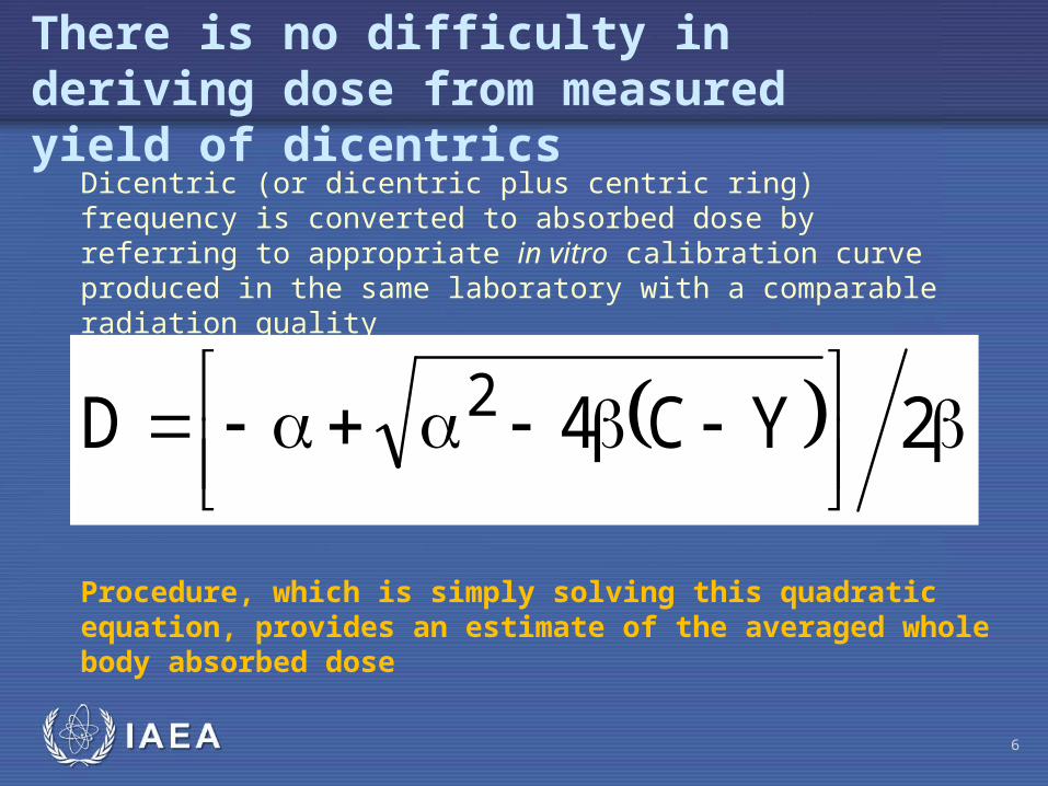
Dicentric (or dicentric plus centric ring) frequency is converted to absorbed dose by referring to appropriate in vitro calibration curve produced in the same laboratory with a comparable radiation quality

2YC4D 2

There is no difficulty in deriving dose from measured yield of dicentrics

Procedure, which is simply solving this quadratic equation, provides an estimate of the averaged whole body absorbed dose

6

IAEA

• There are a number of different ways in which the uncertainty on the yield can be derived

• Aim is to express uncertainty in terms of a confidence interval and it is standard practice to calculate 95% limits

• 95% confidence limits define interval that will encompass true dose on at least 95% of occasions

Difficulty comes when one wishes to determine the uncertainty on dose estimate

7

IAEA

There is no absolute method for deriving confidence limits – it is always approximation

• Uncertainties on calibration curve are distributed as normal probability function

• Uncertainties on measured aberration yield are usually Poissonian or overdispersed

• Difficulty in computation of confidence limits arises because there are two components to uncertainty

8

IAEA

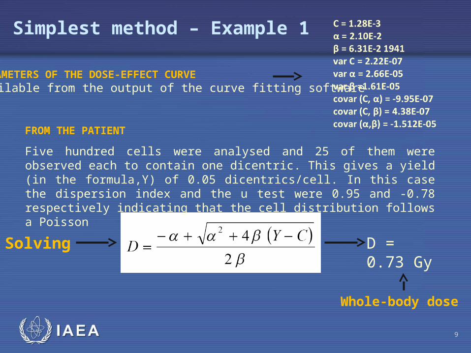
PARAMETERS OF THE DOSE-EFFECT CURVEAvailable from the output of the curve fitting software

FROM THE PATIENT

Five hundred cells were analysed and 25 of them were observed each to contain one dicentric. This gives a yield (in the formula,Y) of 0.05 dicentrics/cell. In this case the dispersion index and the u test were 0.95 and -0.78 respectively indicating that the cell distribution follows a Poisson

Solving D = 0.73 Gy

Whole-body dose

Simplest method – Example 1

9

IAEA

From observed yield of dicentrics and assuming the Poisson distribution, calculate yields corresponding to lower and upper 95% confidence limits on patient’s dicentric yield (YL and YU)

Simplest method – Example 2

10

IAEA

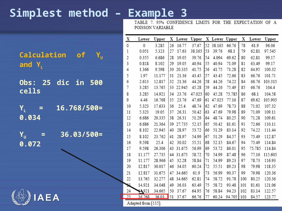
Calculation of YU and YL

Obs: 25 dic in 500 cells

YL = 16.768/500= 0.034

YU = 36.03/500= 0.072

Simplest method – Example 3

11

IAEA

If u test statistic is higher than 1.96, YU and YL should be corrected by multiplying by a factor

Where CL is Poisson confidence limit taken from standard table, X number of dicentrics observed, and σ2/y observed dispersion index

Using same example, if instead of 25 cells with one dicentric, 19 cells with one dicentric and three cells with two were observed then the σ2/y will be 1.19, and the u value +3.19. In his case YU and YL are:

Simplest method – Example 4

12

IAEA

To calculate dose at which YL intercepts upper curve. This is lower confidence limit (DL) on dose estimate. To calculate dose at which YU intercepts lower curve. This is upper confidence limit (DU).

Simplest method – Example 5

13

IAEA

upper curveYL=16.768/500=0.034

lower curveYU = 36.03/500= 0.072

Calculation of point where YL and YU intercept upper and lower confidence curve, which are DL and DU, can be done by iteration

DL = 0.51Gy

Du = 0.97Gy

Simplest method – Example 6

14

IAEA

With well established calibration curves based on large amount of scoring, variance due to curve is small compared with variance on observed yield from subject and can be ignored. A simpler approximate estimate of DL and DU may be obtained directly from calibration curve, by considering where YL and YU cross solid line

At 0.73 Gy the error associated with the present curve is 0.002. This value is obtained by inserting 0.73 Gy for D in the last term the following equation

15

IAEA

Dose calculations for more complex exposures

• Low dose overexposures• Partial body exposures• Protracted and fractionated exposure

and thankfully, rarely

• Critically accidents

Situations that biodosimetry laboratories regularly encounter

16

IAEA

The low dose detection limit depends on:

1. The background frequency of dicentrics

2. The uncertainties on the coefficients, particularly

3. The number of cells analyzed from the patient

• Generally for low-LET radiation the detection limit is around 100-200 mGy

Low dose overexposure cases

• Because the ICRP recommended annual occupational dose limit is 20 mSv, there is often pressure on cytogenetics to try to resolve suspected low overdoses, perhaps pushing the method beyond its capabilities

17

IAEA

dic = dicentrics; y = frequency of dicentrics, Var= variance; DI= dispersion index (VAR/MEAN); u= Papworth’s u

Partial or whole body exposure?

Whole body irradiation is the simplest scenario to describe mathematically but, normally heterogeneous exposures are more likely

Y= 0.0128+0.021D+0.0631D2

• After whole body dose of 3 Gy gamma and using this curve total of 129 dic are expected to be found in 200 cells

• Expected Poisson dic distribution is shown in this table

• DI is close to 1 and u-test value lies between ±1.96

cells with X dicentrics0 105 1 68 2 22 3 5 4 1

5 0 6 0 7 0 8 0 9 0 10 0 11 0 12 0

13 0 cells 200 dic 129y 0,64

Var 0,65DI 1,01

u 0,05

18

IAEA

How to calculate u-test

N

Xy Frequency 0.64

Variance

1N

yndicnwithcells.....y1dic1withcellsy0dic0withcellsVAR

222

0.65

Dispersion Indexy

VARDI 1.01

X112

1N1y

DIu

X the total number of dicentrics, N the total analyzed cells

U test 0.05

19

IAEA

Partial irradiation

cells with X dicentrics Contaminated0 105 305 1 68 68 2 22 22 3 5 5 4 1 1 5 0 0 6 0 0 7 0 0 8 0 0 9 0 0 10 0 0 11 0 0 12 0 0 13 0 0

cells 200 400 dic 129 129y 0,64 0,32

Var 0,65 0.43DI 1.01 1.33u 0.05 4.61

Contamination with 200 unirradiated cells

Same number of dicentrics in more cells. Frequency is lower, and consequently, if a whole body estimation is done, dose will be lower

u value > 1.96 indicates significant overdispersion

This ‘dilutes’ dicentric frequency with undamaged cells

20

IAEA

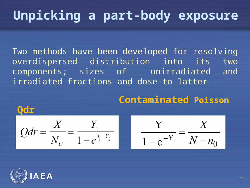
Two methods have been developed for resolving overdispersed distribution into its two components; sizes of unirradiated and irradiated fractions and dose to latter

Unpicking a part-body exposure

Qdr Contaminated Poisson

21

IAEA

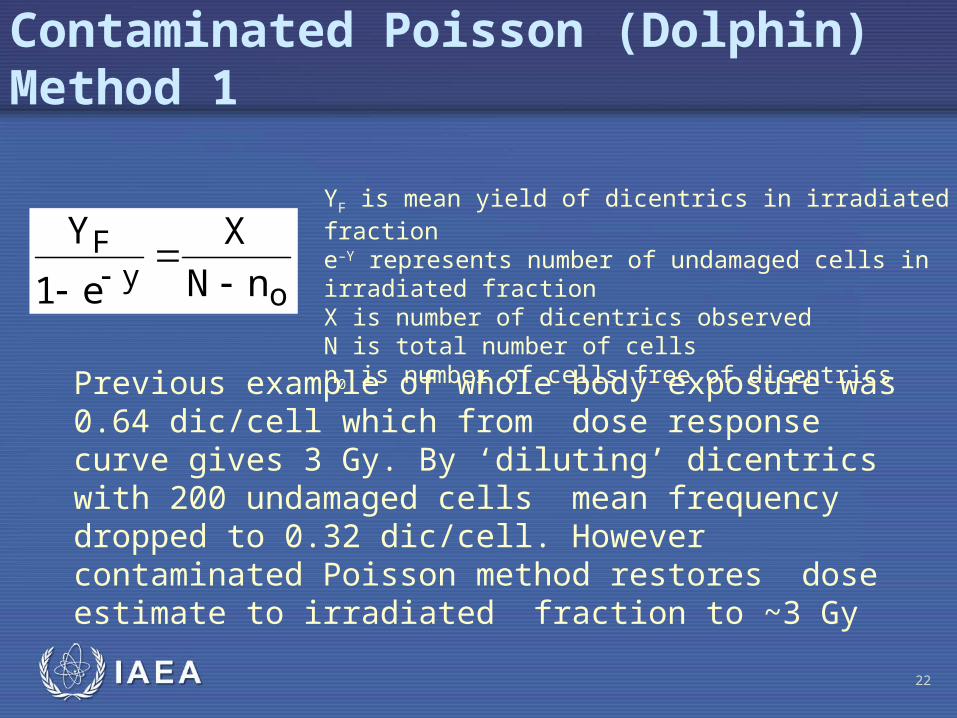
Contaminated Poisson (Dolphin) Method 1

YF is mean yield of dicentrics in irradiated fractione–Y represents number of undamaged cells in irradiated fractionX is number of dicentrics observedN is total number of cellsn0 is number of cells free of dicentrics

oy

F

nN

X

e1

Y

Previous example of whole body exposure was 0.64 dic/cell which from dose response curve gives 3 Gy. By ‘diluting’ dicentrics with 200 undamaged cells mean frequency dropped to 0.32 dic/cell. However contaminated Poisson method restores dose estimate to irradiated fraction to ~3 Gy

22

IAEA

YF can then be used to calculate the fraction, f, of cells scored which were irradiated

Fraction obtained using example is 0.50From 400 cells scored, 200 were non-irradiated

It is also possible to estimate initial fraction of irradiated cells, representing fraction of body irradiated. This calculation takes into account a correction for effects of interphase death and mitotic delayValue p, fraction of irradiated cells that reach metaphase, is estimated

D is estimated dose, and there is experimental evidence of D0 values between 2.7 and 3.5.

Contaminated Poisson (Dolphin) Method 2

23

IAEA

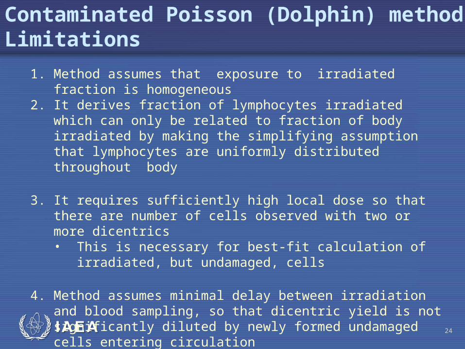
Contaminated Poisson (Dolphin) method Limitations

1. Method assumes that exposure to irradiated fraction is homogeneous

2. It derives fraction of lymphocytes irradiated which can only be related to fraction of body irradiated by making the simplifying assumption that lymphocytes are uniformly distributed throughout body

3. It requires sufficiently high local dose so that there are number of cells observed with two or more dicentrics• This is necessary for best-fit calculation of irradiated, but

undamaged, cells

4. Method assumes minimal delay between irradiation and blood sampling, so that dicentric yield is not significantly diluted by newly formed undamaged cells entering circulation

24

IAEA

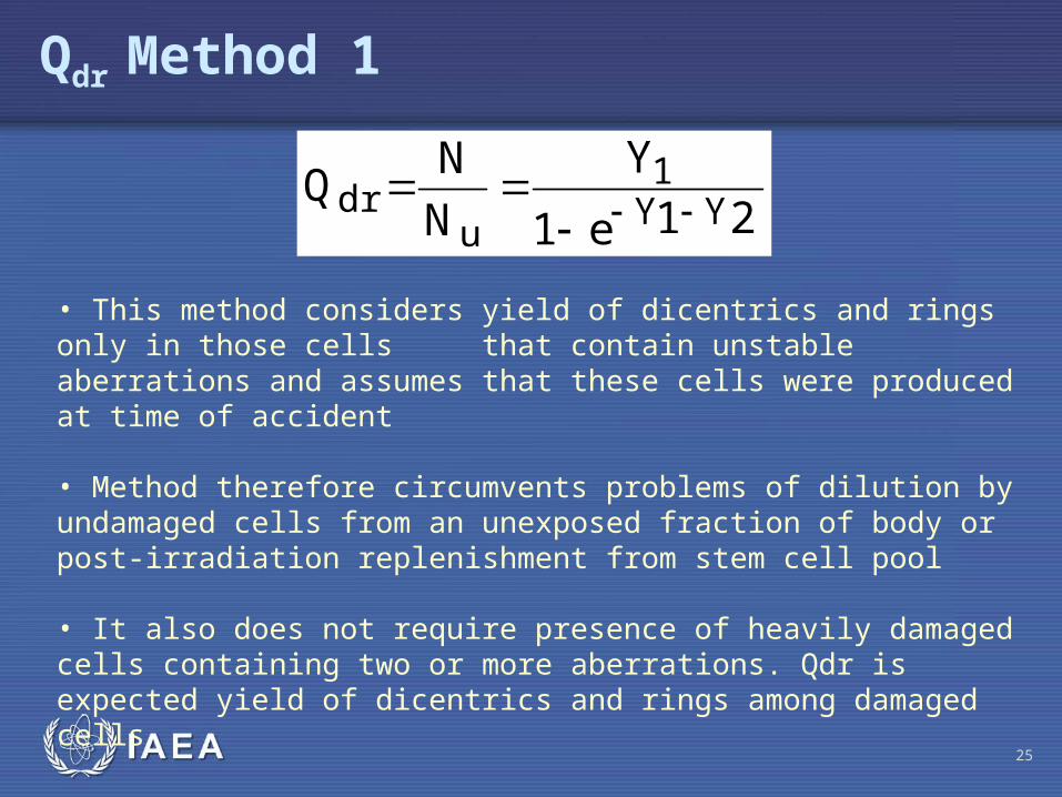
Qdr Method 1

• This method considers yield of dicentrics and rings only in those cells that contain unstable aberrations and assumes that these cells were produced at time of accident

• Method therefore circumvents problems of dilution by undamaged cells from an unexposed fraction of body or post-irradiation replenishment from stem cell pool

• It also does not require presence of heavily damaged cells containing two or more aberrations. Qdr is expected yield of dicentrics and rings among damaged cells

21e1

Y

N

NQ

YY1

udr

25

IAEA

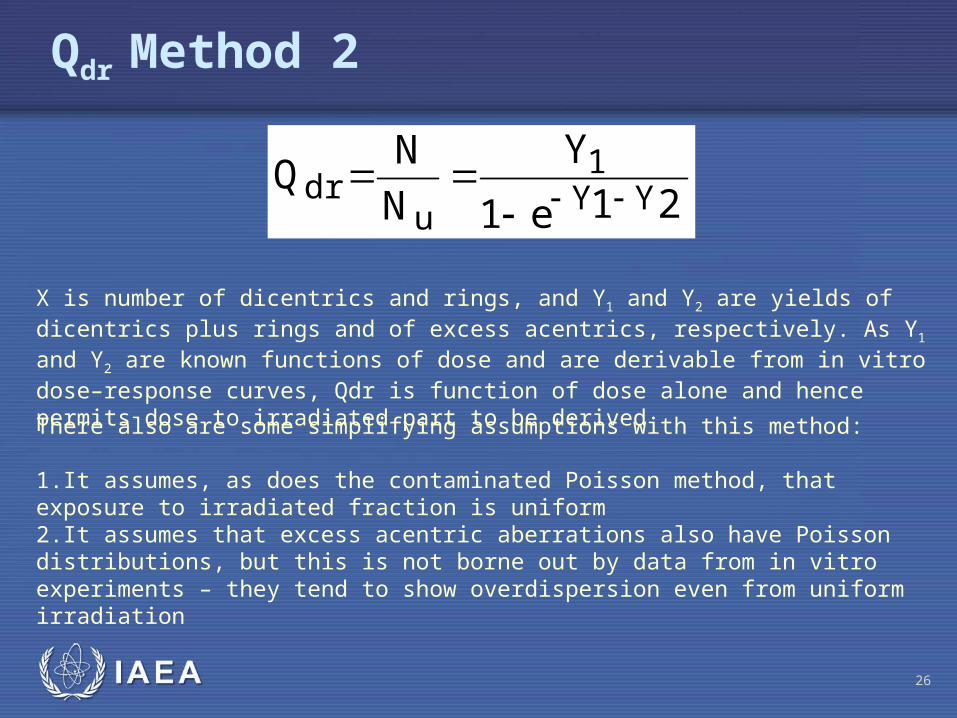
Qdr Method 2

X is number of dicentrics and rings, and Y1 and Y2 are yields of dicentrics plus rings and of excess acentrics, respectively. As Y1 and Y2 are known functions of dose and are derivable from in vitro dose–response curves, Qdr is function of dose alone and hence permits dose to irradiated part to be derived

21e1

Y

N

NQ

YY1

udr

There also are some simplifying assumptions with this method:

1.It assumes, as does the contaminated Poisson method, that exposure to irradiated fraction is uniform2.It assumes that excess acentric aberrations also have Poisson distributions, but this is not borne out by data from in vitro experiments – they tend to show overdispersion even from uniform irradiation

26

IAEA

Protracted and fractionated exposure (1)

• For high LET radiation, where dose–response relationship is close to linear, no dose rate or fractionation effect would be expected

• For low LET radiation, however, effect of dose protraction is to reduce dose squared coefficient, β of linear-quadratic equation

• This term represents those aberrations, possibly of two track origin, which can be modified by repair mechanisms that have time to operate during protracted exposure or in periods between intermittent acute exposures

Protraction or fractionation of a low LET exposure produces lower chromosome aberration yield than same acute dose

27

IAEA

• For brief intermittent exposures, where interfraction intervals of more than six hours are involved, exposures may be considered as number of isolated acute irradiations for each of which induced aberration yields are additive

• Number of studies have shown that decrease in frequencies of aberrations appears to follow single exponential function with mean time of about 2 h

• Time dependent factor known as G function was proposed to enable modification of dose squared coefficient (β) and thus allow for effects of dose protraction

Protracted and fractionated exposure (2)

28

IAEA

t is time over which irradiation occurred

t0 is mean lifetime of breaks (about 2 h)

Protracted and fractionated exposure (3) G-function

G function modifying β coefficient

29

IAEA

Protracted and fractionated exposure (4) G-function example

Using curve parameters

If 25 dicentrics are scored in 500 cells for 24 hours accidental exposure of person:

122

24y

153.0G

2GDDCY 2E96.0G Solving D = 1.41 Gy

This protracted dose is higher than what would be estimated for same dicentric frequency due to acute exposure, 0.73 Gy

30

IAEA

Criticality accident

Body is irradiated by both fission neutrons and gamma raysIf ratio of neutron to gamma ray doses is known (this information is usually available from physical measurements) it is possible to estimate separate neutron and gamma ray doses by iteration

The iteration process is:

(1) Assume that all aberrations are attributable to neutrons, and from measured yield of dicentrics estimate dose from neutron curve

(2) Use estimated neutron dose and supplied neutron to gamma ray ratio to estimate gamma ray dose

(3) Use gamma ray dose to estimate yield of dicentrics due to gamma rays

(4) Subtract this calculated gamma ray yield of dicentrics from measured yield to give new value for neutron yield

(5) Repeat steps 1 to 4 until self-consistent estimates are obtained

31

IAEA

After critically accident 120 dicentrics have been observed in 100 cells (1.2 dic/cell). Neutron to gamma ratio, from physics, is 2:3 in absorbed dose. Using two dose effect curves for neutrons and gamma rays respectively:

Neutrons Y=0.005 +8.32x10-1D

(1) 1.20 dic/cell is equivalent to 1.442 Gy neutrons

(2) 1.442 Gy x (3/2) = 2.163 Gy γ- rays

(3) 2.163 Gy γ- rays are equivalent to 0.266 dic/cell

(4) 1.20-0.266=0.934 dicentric yield attributable to neutrons

γ- rays Y=0.005 + 1.64x10-2D + 4.92x10-2D2

(5) 0.934 dic/cell is equivalent to 1.122 Gy neutrons

Repeating stage 2, 1.122 x3/2 = 1.683 Gy γ-rays. After a few iterations estimated doses are 1.21 Gy for neutrons and 1.82 Gy for γ-rays

dic/cell Iteration Doses dic equivalent to γ-rays1,200 1 Dose N 1,442

Dose γ 2,163 0,2660,934 2 Dose N 1,122

Dose γ 1,683 0,1671,033 3 Dose N 1,240

Dose γ 1,861 0,2010,999 4 Dose N 1,200

Dose γ 1,800 0,1891,011 5 Dose N 1,214

Dose γ 1,821 0,1941,006 6 Dose N 1,209

Dose γ 1,814 0,1921,008 7 Dose N 1,211

Dose γ 1,816 0,1931,007 8 Dose N 1,210

Dose γ 1,815 0,1921,008 9 Dose N 1,210

Dose γ 1,816 0,192

Criticality accident – Example

32

IAEA

Final comment

• Don’t panic about doing statistics and calculations

• It is more important that you understand principles of how to estimate dose uncertainties and how to deal with complications such as inhomogeneity, dose protraction and mixed radiations

• For example, if you see overdispersion don’t just give the averaged dose

• User friendly, freely available software packages: CABAS and Dose Estimate could assist

33