I.3 FILES IN MATLAB

I.3.1 Why do we need M-Files?

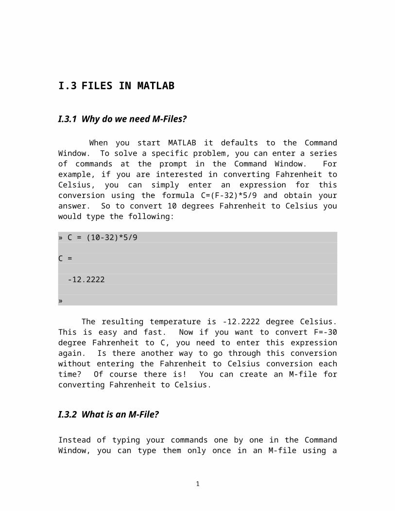
When you start MATLAB it defaults to the Command Window. To solve a specific problem, you can enter a series of commands at the prompt in the Command Window. For example, if you are interested in converting Fahrenheit to Celsius, you can simply enter an expression for this conversion using the formula C=(F-32)*5/9 and obtain your answer. So to convert 10 degrees Fahrenheit to Celsius you would type the following:

» C = (10-32)*5/9

C =

-12.2222

»

The resulting temperature is -12.2222 degree Celsius. This is easy and fast. Now if you want to convert F=-30 degree Fahrenheit to C, you need to enter this expression again. Is there another way to go through this conversion without entering the Fahrenheit to Celsius conversion each time? Of course there is! You can create an M-file for converting Fahrenheit to Celsius.

I.3.2 What is an M-File?

Instead of typing your commands one by one in the Command Window, you can type them only once in an M-file using a text editor of your choice. When you tell MATLAB to run your M-file, it will open the file and evaluate commands in the sequence appearing in the file.

RememberM-File filename must end with the extension ‘.m’

These files are called script files, or simply M-files. The term “script” emphasizes the fact that MATLAB simply reads from the “script” found in the file. The term “M-file” recognizes the fact that script filenames must end with the extension “.m”, e.g., f_to_c.m.

1

RememberAn M-file consists of a sequence of MATLAB command statements

All M-files are either in script or function form. Scripts are suitable when you need to perform a long sequence of commands. Function files, on the other hand, have more flexibility, as they allow the user to pass and return values as would with other MATLAB functions.

RememberThere are two types of MATLAB M-files: script and function files

I.3.3 How to Create and Edit an M-file?

RememberSteps involved in working with MATLAB M-files are:

CREATE à EDIT à RUN

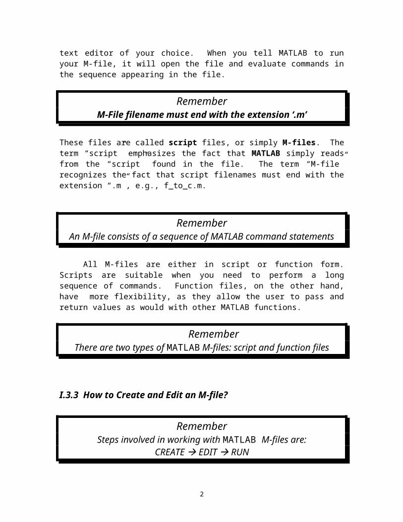
M-Files are ASCII files that can be created using a text editor or word processor. To create a new M-file, choose New from the File menu and then select M-file.

This procedure will open a default text editor where you can begin entering your MATLAB commands. If you like to add comments to your code, you may do so by starting the “comment” line with a “%” character. Once you have finished entering your commands, you must save your file. To save your file, choose Save As from the File menu of the text editor.

2

RememberYou must save your MATLAB M-files with .m extensions

Once you have created your M-file, you can execute it by either typing the name of the M-file at the command prompt in the Command Window or by choosing Run M-File (Script File) from the File menu in the Command Window.

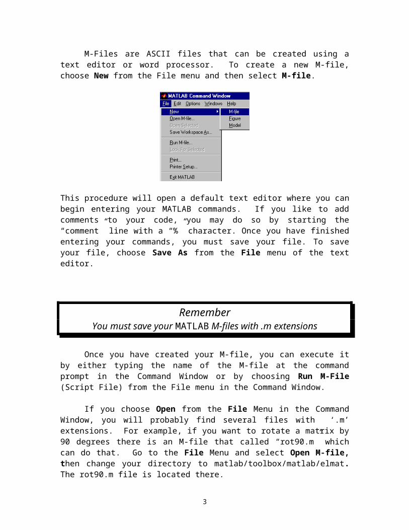
If you choose Open from the File Menu in the Command Window, you will

probably find several files with ‘.m’ extensions. For example, if you want to rotate a matrix by 90 degrees there is an M-file that called “rot90.m” which can do that. Go to the File Menu and select Open M-file, then change your directory to matlab/toolbox/matlab/elmat. The rot90.m file is located there.

This brings up the question of locating both user written M-files and built-in MATLAB functions. Suppose you wanted to do a matrix rotation with the function rot90.m, but you do not know where it is located. The function which {M-file} will search through the MATLAB path and give you the location of the desired M-file. For example, to find the location of the function rot90.m, you can enter:

» which rot90

c:\matlab\toolbox\matlab\elmat\rot90.m

Occasionally, one forgets the name of an M-file to do a certain task. Or one may want to search for a selection of similar MATLAB capabilities. You can use the lookfor {keyword} command, which will give you a list of M-files that relate to a given keyword. For example, if you wanted a list of all the M-files that have anything to do with the word "rotate," you would enter:

3

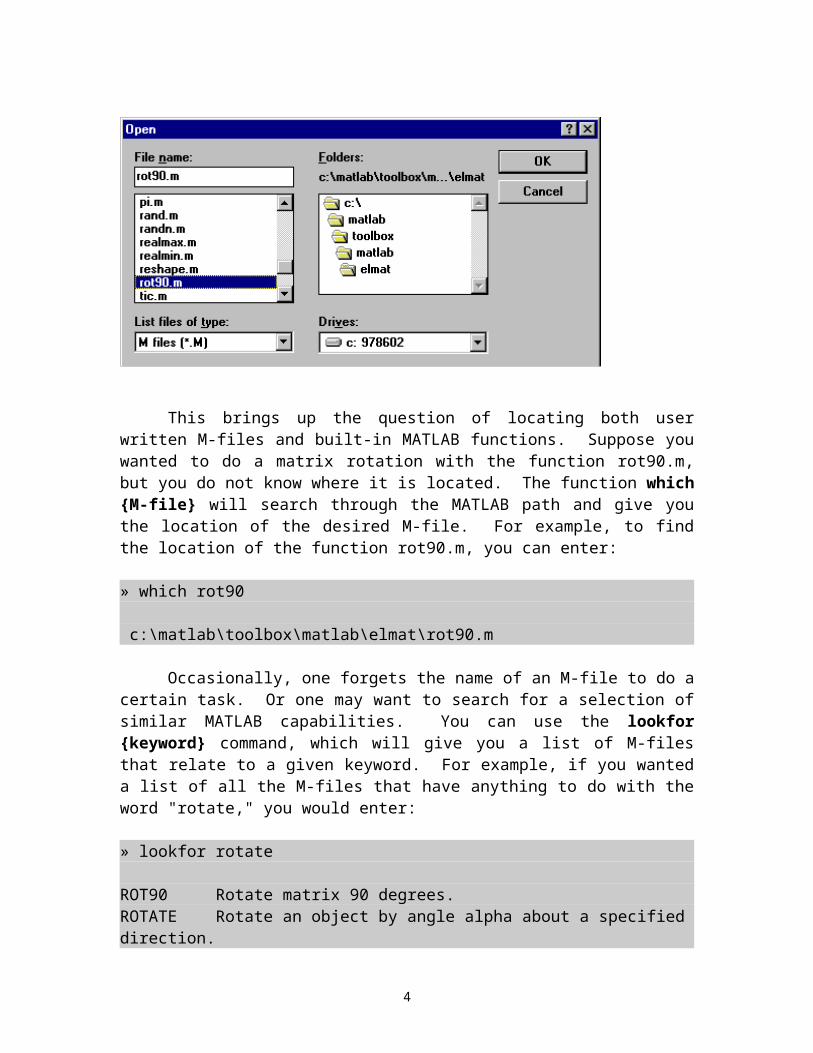
» lookfor rotate

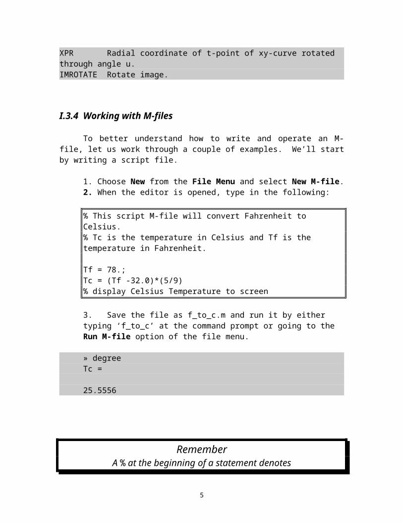
ROT90 Rotate matrix 90 degrees.ROTATE Rotate an object by angle alpha about a specified direction.XPR Radial coordinate of t-point of xy-curve rotated through angle u.IMROTATE Rotate image.

I.3.4 Working with M-files

To better understand how to write and operate an M-file, let us work through a couple of examples. We’ll start by writing a script file.

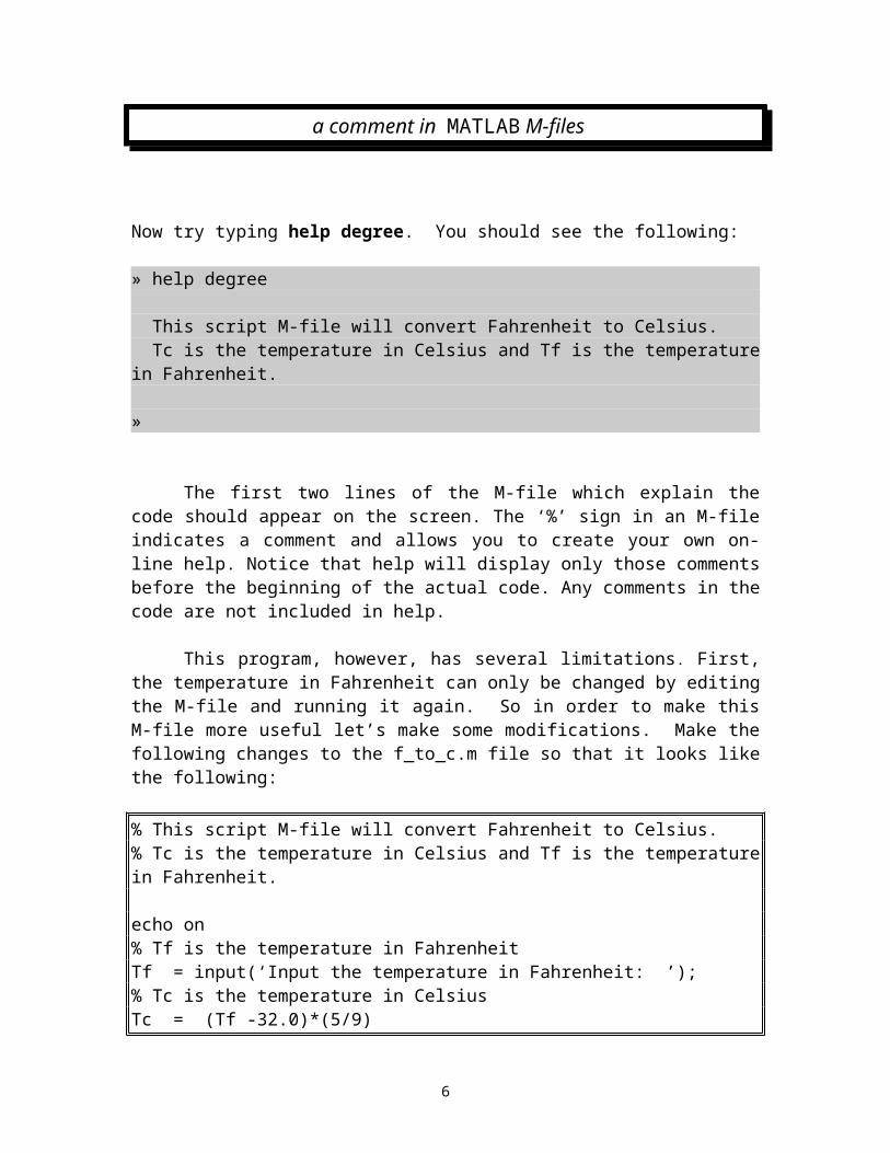
1. Choose New from the File Menu and select New M-file.2. When the editor is opened, type in the following:

% This script M-file will convert Fahrenheit to Celsius.% Tc is the temperature in Celsius and Tf is the temperature in Fahrenheit.

Tf = 78.;Tc = (Tf -32.0)*(5/9)% display Celsius Temperature to screen

3. Save the file as f_to_c.m and run it by either typing ‘f_to_c’ at the command prompt or going to the Run M-file option of the file menu.

» degreeTc =

25.5556

RememberA % at the beginning of a statement denotes

a comment in MATLAB M-files

Now try typing help degree. You should see the following:

4

» help degree

This script M-file will convert Fahrenheit to Celsius. Tc is the temperature in Celsius and Tf is the temperature in Fahrenheit.

»

The first two lines of the M-file which explain the code should appear on the screen. The ‘%’ sign in an M-file indicates a comment and allows you to create your own on-line help. Notice that help will display only those comments before the beginning of the actual code. Any comments in the code are not included in help.

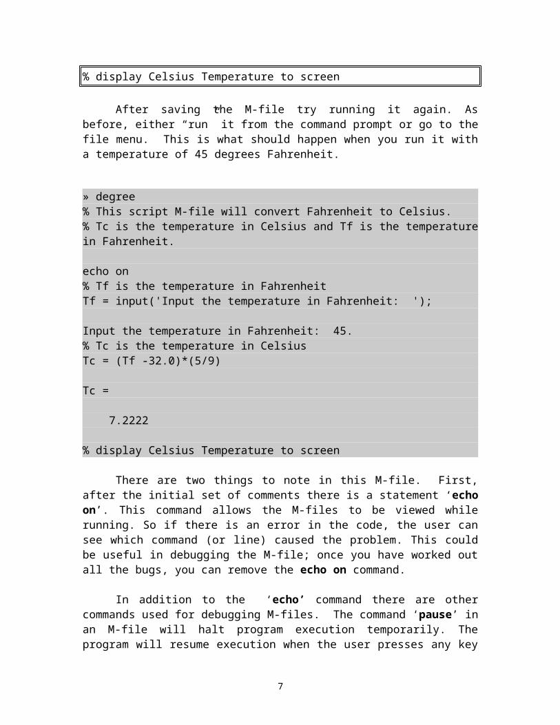
This program, however, has several limitations. First, the temperature in Fahrenheit can only be changed by editing the M-file and running it again. So in order to make this M-file more useful let’s make some modifications. Make the following changes to the f_to_c.m file so that it looks like the following:

% This script M-file will convert Fahrenheit to Celsius.% Tc is the temperature in Celsius and Tf is the temperature in Fahrenheit.

echo on% Tf is the temperature in FahrenheitTf = input(‘Input the temperature in Fahrenheit: ’);% Tc is the temperature in CelsiusTc = (Tf -32.0)*(5/9)% display Celsius Temperature to screen

After saving the M-file try running it again. As before, either “run” it from the command prompt or go to the file menu. This is what should happen when you run it with a temperature of 45 degrees Fahrenheit.

» degree% This script M-file will convert Fahrenheit to Celsius.% Tc is the temperature in Celsius and Tf is the temperature in Fahrenheit.

echo on% Tf is the temperature in FahrenheitTf = input('Input the temperature in Fahrenheit: ');

Input the temperature in Fahrenheit: 45.% Tc is the temperature in CelsiusTc = (Tf -32.0)*(5/9)

Tc =

5

7.2222

% display Celsius Temperature to screen

There are two things to note in this M-file. First, after the initial set of comments there is a statement ‘echo on’. This command allows the M-files to be viewed while running. So if there is an error in the code, the user can see which command (or line) caused the problem. This could be useful in debugging the M-file; once you have worked out all the bugs, you can remove the echo on command.

In addition to the ‘echo’ command there are other commands used for debugging M-files. The command ‘pause’ in an M-file will halt program execution temporarily. The program will resume execution when the user presses any key on the keyboard. Similarly, ‘pause(n)’ will cause the program to stop for n seconds. There is another command called keyboard which is used in M-file debugging and modification. When used in an M-file, it invokes the keyboard as if it were a script M-file. During execution of an M-file, the keyboard command halts execution, allowing the user to modify or observe the contents of MATLAB variables. Upon execution of the keyboard command, MATLAB is placed in the Keyboard mode, which is noted by a ‘K>>’ prompt appearing in the Command Window. The Keyboard mode can only be exited by typing ‘return’ and then pressing the Enter key to resume execution.

A second point of note in the above M-file is that the MATLAB variable Tf is now an input from the user. When the M-file was run, the user was prompted for the temperature. After entering the desired value and then pressing return, the program finished executing and displayed the result. Script files are just an example of M-files. As mentioned previously, M-files can also be in the form of functions. Function M-files can easily be differentiated from script files since the word function always appears first in a function M-file. Function files also allow values to be passed into the M-files. To explain the implementation of function M-files we will work through another example.

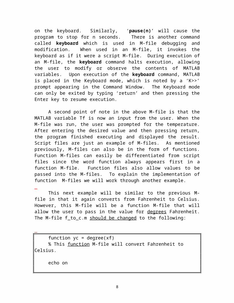
This next example will be similar to the previous M-file in that it again converts from Fahrenheit to Celsius. However, this M-file will be a function M-file that will allow the user to pass in the value for degrees Fahrenheit. The M-file f_to_c.m should be changed to the following:

function yc = degree(xf)% This function M-file will convert Fahrenheit to Celsius.

echo on

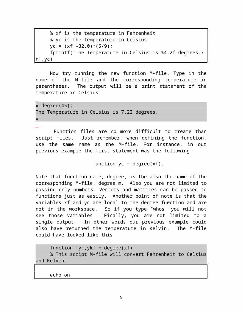
% xf is the temperature in Fahrenheit% yc is the temperature in Celsius

6

yc = (xf -32.0)*(5/9);fprintf(‘The Temperature in Celsius is %4.2f degrees.\n’,yc)

Now try running the new function M-file. Type in the name of the M-file and the corresponding temperature in parentheses. The output will be a print statement of the temperature in Celsius. » degree(45);The Temperature in Celsius is 7.22 degrees.»

Function files are no more difficult to create than script files. Just remember, when defining the function, use the same name as the M-file. For instance, in our previous example the first statement was the following:

function yc = degree(xf).

Note that function name, degree, is the also the name of the corresponding M-file, degree.m. Also you are not limited to passing only numbers. Vectors and matrices can be passed to functions just as easily. Another point of note is that the variables xf and yc are local to the degree function and are not in the workspace. So if you type “whos” you will not see those variables. Finally, you are not limited to a single output. In other words our previous example could also have returned the temperature in Kelvin. The M-file could have looked like this.

function [yc,yk] = degree(xf)% This script M-file will convert Fahrenheit to Celsius and Kelvin.

echo on

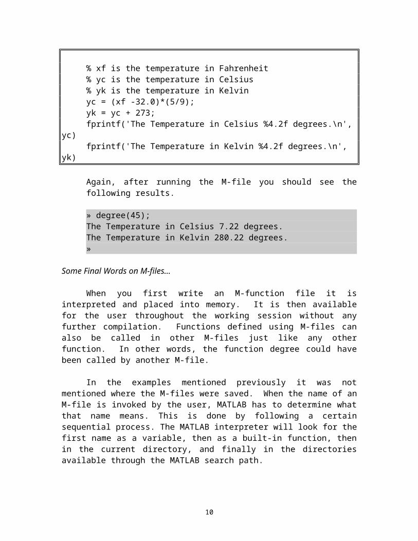
% xf is the temperature in Fahrenheit% yc is the temperature in Celsius% yk is the temperature in Kelvinyc = (xf -32.0)*(5/9);yk = yc + 273;fprintf('The Temperature in Celsius %4.2f degrees.\n', yc)fprintf('The Temperature in Kelvin %4.2f degrees.\n', yk)

Again, after running the M-file you should see the following results.

» degree(45);The Temperature in Celsius 7.22 degrees.The Temperature in Kelvin 280.22 degrees.»

7

Some Final Words on M-files…

When you first write an M-function file it is interpreted and placed into memory. It is then available for the user throughout the working session without any further compilation. Functions defined using M-files can also be called in other M-files just like any other function. In other words, the function degree could have been called by another M-file.

In the examples mentioned previously it was not mentioned where the M-files were saved. When the name of an M-file is invoked by the user, MATLAB has to determine what that name means. This is done by following a certain sequential process. The MATLAB interpreter will look for the first name as a variable, then as a built-in function, then in the current directory, and finally in the directories available through the MATLAB search path.

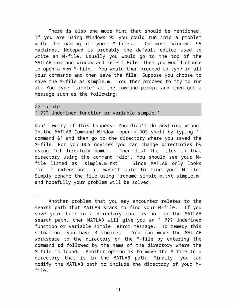
There is also one more hint that should be mentioned. If you are using Windows 95 you could run into a problem with the naming of your M-files. On most Windows 95 machines, Notepad is probably the default editor used to write an M-file. Usually you would go to the top of the MATLAB Command Window and select File. Then you would choose to open a new M-file. You would then proceed to type in all your commands and then save the file. Suppose you choose to save the M-file as simple.m. You then proceed to try to run it. You type ‘simple’ at the command prompt and then get a message such as the following:

>> simple‘ ??? Undefined function or variable simple.’ Don’t worry if this happens. You didn’t do anything wrong. In the MATLAB Command Window, open a DOS shell by typing ‘!command &’ and then go to the directory where you saved the M-file. For you DOS novices you can change directories by using ‘cd directory name’. Then list the files in that directory using the command ‘dir’. You should see your M-file listed as ‘simple.m.txt’. Since MATLAB only looks for .m extensions, it wasn’t able to find your M-file. Simply rename the file using ‘rename simple.m.txt simple.m’ and hopefully your problem will be solved.

Another problem that you may encounter relates to the search path that MATLAB

scans to find your M-file. If you save your file in a directory that is not in the MATLAB search path, then MATLAB will give you an ‘ ??? Undefined function or variable simple’ error message. To remedy this situation, you have 3 choices. You can move the MATLAB workspace to the directory of the M-file by entering the command cd followed by the name of the directory where the M-file is found. Another option is to move the M-file to a directory that is in the MATLAB path. Finally, you can modify the MATLAB path to include the directory of your M-file.

8

I.3.5 Saving Workspaces

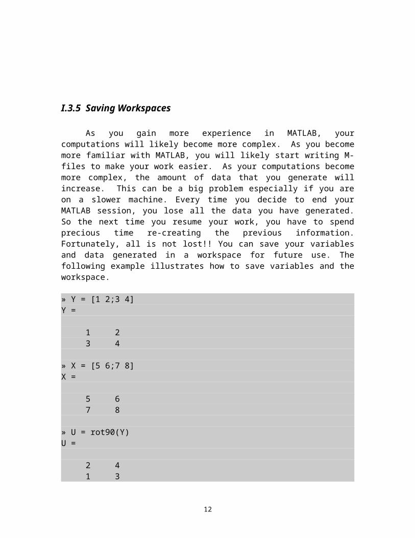
As you gain more experience in MATLAB, your computations will likely become more complex. As you become more familiar with MATLAB, you will likely start writing M-files to make your work easier. As your computations become more complex, the amount of data that you generate will increase. This can be a big problem especially if you are on a slower machine. Every time you decide to end your MATLAB session, you lose all the data you have generated. So the next time you resume your work, you have to spend precious time re-creating the previous information. Fortunately, all is not lost!! You can save your variables and data generated in a workspace for future use. The following example illustrates how to save variables and the workspace.

» Y = [1 2;3 4]Y =

1 2 3 4

» X = [5 6;7 8]X =

5 6 7 8

» U = rot90(Y)U =

2 4 1 3

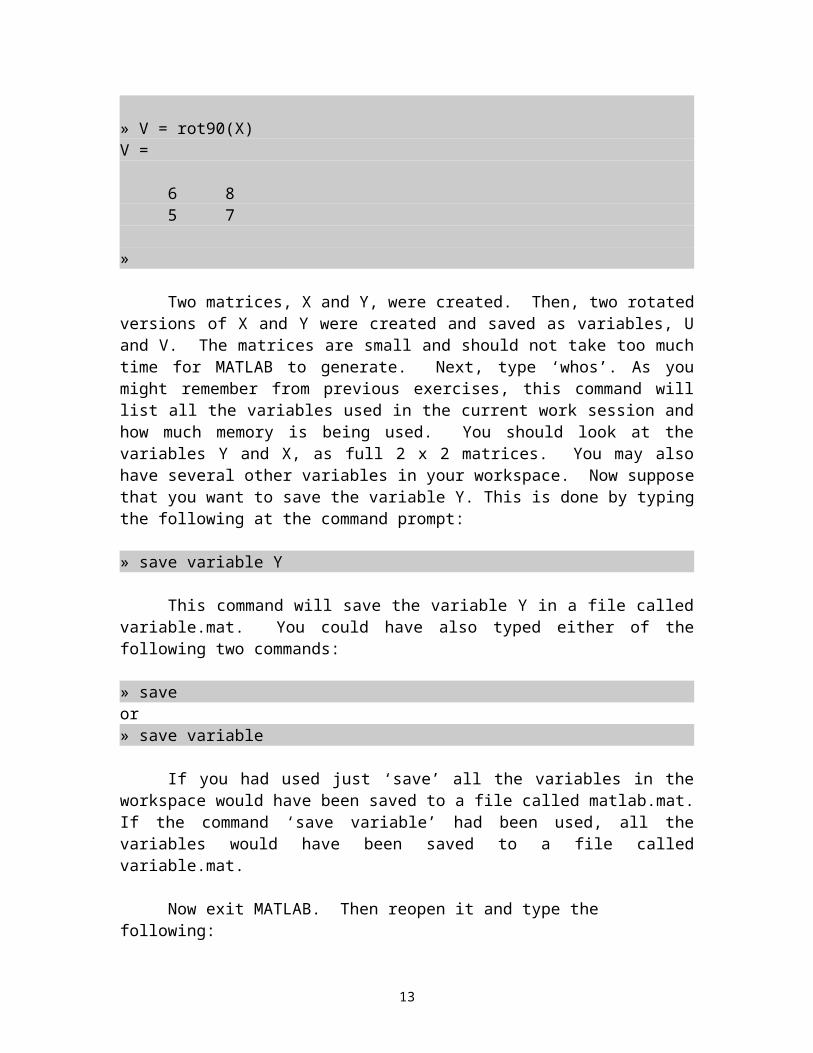
» V = rot90(X)V =

6 8 5 7

»

Two matrices, X and Y, were created. Then, two rotated versions of X and Y were created and saved as variables, U and V. The matrices are small and should not take too much time for MATLAB to generate. Next, type ‘whos’. As you might remember from previous exercises, this command will list all the variables used in the current work session and how much memory is being used. You should look at the

9

variables Y and X, as full 2 x 2 matrices. You may also have several other variables in your workspace. Now suppose that you want to save the variable Y. This is done by typing the following at the command prompt:

» save variable Y

This command will save the variable Y in a file called variable.mat. You could have also typed either of the following two commands:

» save or » save variable

If you had used just ‘save’ all the variables in the workspace would have been saved to a file called matlab.mat. If the command ‘save variable’ had been used, all the variables would have been saved to a file called variable.mat.

Now exit MATLAB. Then reopen it and type the following:

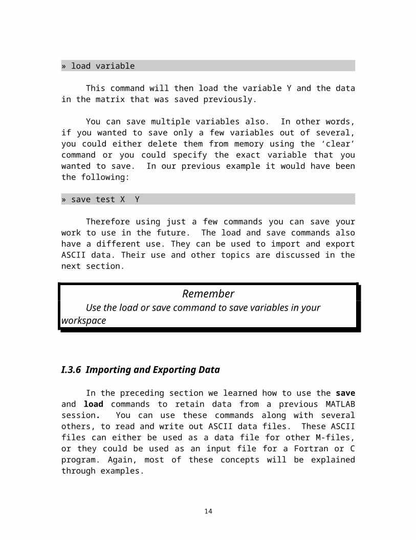
» load variable

This command will then load the variable Y and the data in the matrix that was saved previously.

You can save multiple variables also. In other words, if you wanted to save only a few variables out of several, you could either delete them from memory using the ‘clear’ command or you could specify the exact variable that you wanted to save. In our previous example it would have been the following:

» save test X Y

Therefore using just a few commands you can save your work to use in the future. The load and save commands also have a different use. They can be used to import and export ASCII data. Their use and other topics are discussed in the next section.

RememberUse the load or save command to save variables in your workspace

I.3.6 Importing and Exporting Data

10

In the preceding section we learned how to use the save and load commands to retain data from a previous MATLAB session. You can use these commands along with several others, to read and write out ASCII data files. These ASCII files can either be used as a data file for other M-files, or they could be used as an input file for a Fortran or C program. Again, most of these concepts will be explained through examples.

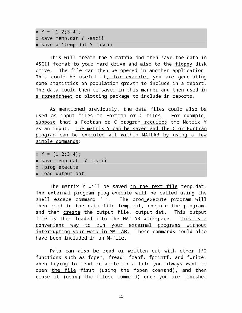
» Y = [1 2;3 4];» save temp.dat Y -ascii» save a:\temp.dat Y -ascii

This will create the Y matrix and then save the data in ASCII format to your hard

drive and also to the floppy disk drive. The file can then be opened in another application. This could be useful if, for example, you are generating some statistics on population growth to include in a report. The data could then be saved in this manner and then used in a spreadsheet or plotting package to include in reports.

As mentioned previously, the data files could also be used as input files to Fortran

or C files. For example, suppose that a Fortran or C program requires the Matrix Y as an input. The matrix Y can be saved and the C or Fortran program can be executed all within MATLAB by using a few simple commands:

» Y = [1 2;3 4];» save temp.dat Y -ascii» !prog_execute» load output.dat

The matrix Y will be saved in the text file temp.dat. The external program

prog_execute will be called using the shell escape command ’!’. The prog_execute program will then read in the data file temp.dat, execute the program, and then create the output file, output.dat. This output file is then loaded into the MATLAB workspace. This is a convenient way to run your external programs without interrupting your work in MATLAB. These commands could also have been included in an M-file.

Data can also be read or written out with other I/O functions such as fopen, fread,

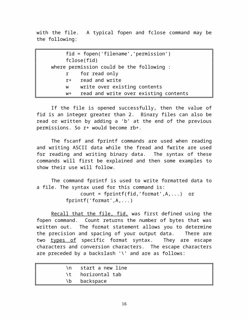
fcanf, fprintf, and fwrite. When trying to read or write to a file you always want to open the file first (using the fopen command), and then close it (using the fclose command) once you are finished with the file. A typical fopen and fclose command may be the following:

fid = fopen(‘filename’,’permission’)fclose(fid)

where permission could be the following :r for read onlyr+ read and writew write over existing contents

11

w+ read and write over existing contents

If the file is opened successfully, then the value of fid is an integer greater than 2. Binary files can also be read or written by adding a ‘b’ at the end of the previous permissions. So r+ would become rb+.

The fscanf and fprintf commands are used when reading and writing ASCII data while the fread and fwrite are used for reading and writing binary data. The syntax of these commands will first be explained and then some examples to show their use will follow.

The command fprintf is used to write formatted data to a file. The syntax used for

this command is:count = fprintf(fid,’format’,A,...) or fprintf(‘format’,A,...)

Recall that the file, fid, was first defined using the fopen command. Count

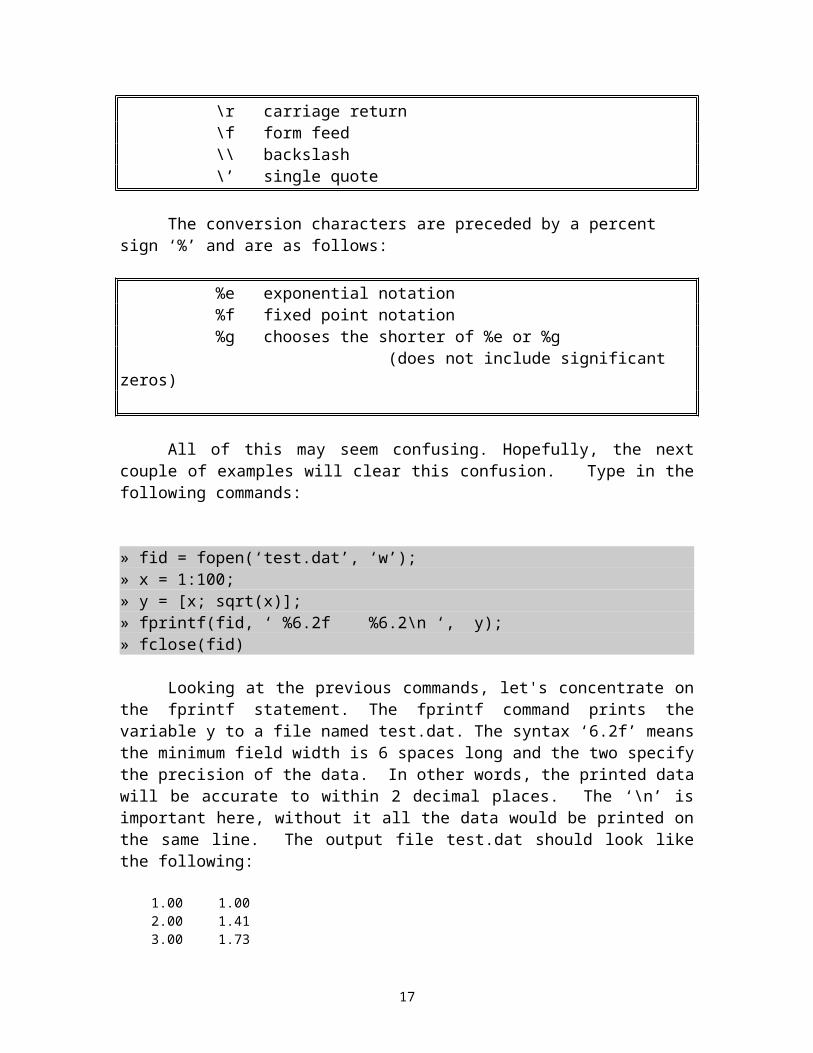
returns the number of bytes that was written out. The format statement allows you to determine the precision and spacing of your output data. There are two types of specific format syntax. They are escape characters and conversion characters. The escape characters are preceded by a backslash ‘\’ and are as follows:

\n start a new line\t horizontal tab\b backspace\r carriage return\f form feed\\ backslash\’ single quote

The conversion characters are preceded by a percent sign ‘%’ and are as follows:

%e exponential notation%f fixed point notation%g chooses the shorter of %e or %g

(does not include significant zeros)

All of this may seem confusing. Hopefully, the next couple of examples will clear this confusion. Type in the following commands:

» fid = fopen(‘test.dat’, ‘w’);» x = 1:100;» y = [x; sqrt(x)];» fprintf(fid, ‘ %6.2f %6.2\n ‘, y);

12

» fclose(fid)

Looking at the previous commands, let's concentrate on the fprintf statement. The fprintf command prints the variable y to a file named test.dat. The syntax ‘6.2f’ means the minimum field width is 6 spaces long and the two specify the precision of the data. In other words, the printed data will be accurate to within 2 decimal places. The ‘\n’ is important here, without it all the data would be printed on the same line. The output file test.dat should look like the following:

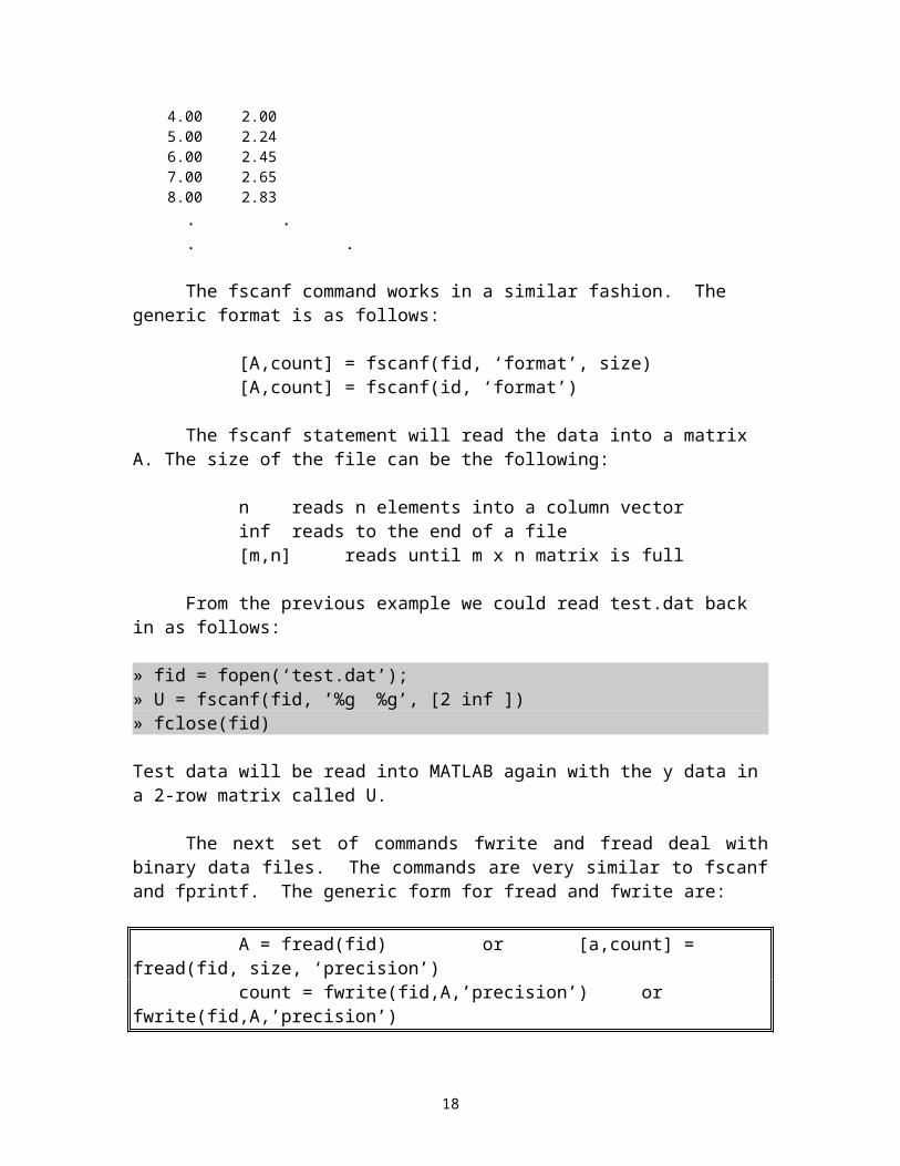
1.00 1.002.00 1.413.00 1.734.00 2.005.00 2.246.00 2.457.00 2.658.00 2.83

. .

. .

The fscanf command works in a similar fashion. The generic format is as follows:

[A,count] = fscanf(fid, ‘format’, size)[A,count] = fscanf(id, ‘format’)

The fscanf statement will read the data into a matrix A. The size of the file can be the following:

n reads n elements into a column vectorinf reads to the end of a file[m,n] reads until m x n matrix is full

From the previous example we could read test.dat back in as follows:

» fid = fopen(‘test.dat’);» U = fscanf(fid, ’%g %g’, [2 inf ])» fclose(fid)

Test data will be read into MATLAB again with the y data in a 2-row matrix called U.

The next set of commands fwrite and fread deal with binary data files. The commands are very similar to fscanf and fprintf. The generic form for fread and fwrite are:

A = fread(fid) or [a,count] = fread(fid, size, ‘precision’)

13

count = fwrite(fid,A,’precision’) or fwrite(fid,A,’precision’)

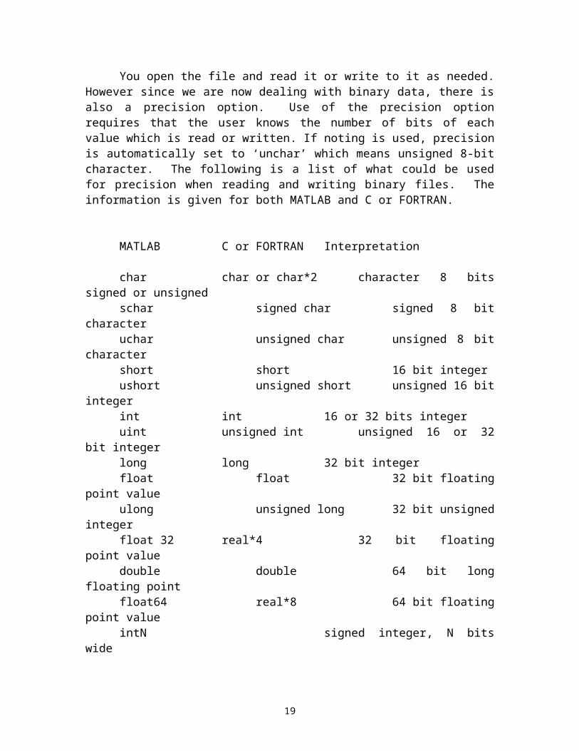
You open the file and read it or write to it as needed. However since we are now dealing with binary data, there is also a precision option. Use of the precision option requires that the user knows the number of bits of each value which is read or written. If noting is used, precision is automatically set to ‘unchar’ which means unsigned 8-bit character. The following is a list of what could be used for precision when reading and writing binary files. The information is given for both MATLAB and C or FORTRAN.

MATLAB C or FORTRAN Interpretation

char char or char*2 character 8 bits signed or unsignedschar signed char signed 8 bit characteruchar unsigned char unsigned 8 bit charactershort short 16 bit integerushort unsigned short unsigned 16 bit integerint int 16 or 32 bits integeruint unsigned int unsigned 16 or 32 bit integerlong long 32 bit integerfloat float 32 bit floating point valueulong unsigned long 32 bit unsigned integerfloat 32 real*4 32 bit floating point valuedouble double 64 bit long floating pointfloat64 real*8 64 bit floating point valueintN signed integer, N bits wideuintN unsigned integer N bits wide

Therefore, using freadf you could read in binary data from C or Fortran. Likewise, you could write binary data that would be compatible with your external program.

I.3.7 Using the MATLAB Debugger

Often times when writing an M-file you will save it and run it only to find that MATLAB either says you have an error or you get values that you weren’t expecting. There are several options at this point. You can start by removing the semicolons so that the data is displayed as it is calculated. If this does not help, the echo and keyboard commands could also be used to examine the workspace state at any point during execution. Finally if you are running the MATLAB version of 4.0 or greater you could use the MATLAB debugger. A list of all the debugging commands are listed in Chapter 1.

14

RememberThe debugger only works on MATLAB function files

To better understand the debugger commands we will work through some

examples. Create the following function M-file shown below:

function [y1,y2] = temp(x)% For each Matrix entered, find the determinant and rotate the matrixy2 = rot90(x) y1 = det(x)

After running the M-file with a matrix you should get results similar to the following:

» x = [3 4 5;1 5 6;7 8 9]x =

3 4 5 1 5 6 7 8 9

» temp(x);y2 =

5 6 9 4 5 8 3 1 7

y1 =

-12

» To start using the debugger, first use the dbtype command. This command will list the M-file with line numbers. The syntax of this command is dbtype followed by the function name. In the following example, the dbtype command will be used for both the temp M-file and the rot90 M-file. After using dbtype you should see the following:

» dbtype temp

1 function [y1,y2] = temp_example(x)2 % For each Matrix entered find the determinant and rotate the matrix3 y2 = rot90(x)

15

4 y1 = det(x)

» dbtype rot90

1 function B = rot90(A,k)2 %ROT90 Rotate matrix 90 degrees.3 % rot90(A) is the 90 degree rotation of m x n matrix A.4 % rot90(A,k) is the k*90 degree rotation of A, k = +-1,+-2,...5 % For example,6 %7 % A = [1 2 3 B = rot90(A) = [ 3 68 % 4 5 6 ] 2 59 % 1 4 ]10 %11 % mesh(B) then shows a 90 degree counter-clockwise rotation12 % of mesh(A).13 %14 % See also VIEW, FLIPUD, FLIPLR.15 16 % From John de Pillis 19 June 198517 % Modified 12-19-91, LS.18 % Copyright (c) 1984-93 by The MathWorks, Inc.19 20 21 [m,n] = size(A);22 if nargin == 123 k = 1;24 else25 k = rem(k,4);26 if k < 027 k = k + 4;28 end29 end30 if k == 131 A = A.';32 B = A(n:-1:1,:);33 elseif k == 234 B = A(m:-1:1,n:-1:1);35 elseif k == 336 B = A(m:-1:1,:);37 B = B.';38 else39 B = A;40 end

»

16

Now we will set a stop in the temp M-file and the rot90 M-file using the following command:

» dbstop at 2 in temp» dbstop at 21 in rot90

These statements will cause MATLAB execution to stop at line 2 in the temp M-

file and at line 21 in the rot90 M-file. Now run the M-file again using a different value of x. You should see something like this.

» x = [2 6 7;3 8 4; 1 6 3];» temp(x);y2 = rot90(x) K»

Execution stopped at line 2 in the temp M-file and is now in the keyboard

command mode. At this time, use the dbstack command to display all the function calls. The command dbstack should return the function and its appropriate path. This is an example of what you may see. Since you may have saved your M-file somewhere else your path may be different than this.

K» dbstackIn c:\matlab\bin\temp.m at line 3K»

At this point you can enter whos to see what variables are being used and what their values are. We will continue execution and move to the next break point using the dbcont command. After typing dbcont you should see something like this.

K» dbcont21 [m,n] = size(A);K»

The dbcont statement allowed the M-file to continue until the next breakpoint. If we wanted to move line by line through our code, we could use the dbstep command. Using the dbstep command in the program we could view the values as the program is being run. The use of the dbstep command is shown below:

K» dbstep22 if nargin == 1K» narginnargin =

1K» dbstep

17

23 k = 1;

K» dbstep24 elseK» k

k =

1

K» At this point we could use dbcont to allow the program to run to completion or

we could step through the entire rot90 M-file line by line. If there are more breakpoints that you do not need anymore, the dbclear command can be used.

K» dbclear at 21 in rot90

The above statement will clear the breakpoint in rot90. If you are satisfied with the results of your M-file and wish to quit the debugger, dbquit will take the user out of the debugging mode.

K» dbquit» Now try running the program temp again; the following should happen.

» temp(x)3 y2 = rot90(x)K» dbconty2 =

7 4 3 6 8 6 2 3 1

y1 = 40

Since all the breakpoints were not cleared, MATLAB again stopped in the temp

M-file and reverted to the debugging mode. You have to clear all stops before quitting the debugger, or you can use the clear command in the workspace. Do be careful, even though the clear command will clear ALL variables.

There were several important topics discussed in this chapter. We learned how

to create, run and debug M-files to make your work easier. We also learned how to read

18

and write data to files. The information provided should cover most of your needs. And of course, practice makes perfect so work through those examples. Remember you can always use the help provided with MATLAB for more information and examples.

19