Uncertain respondents, hypothetical bias, and contingent valuation: The consequences of modeling the wrong decision making process

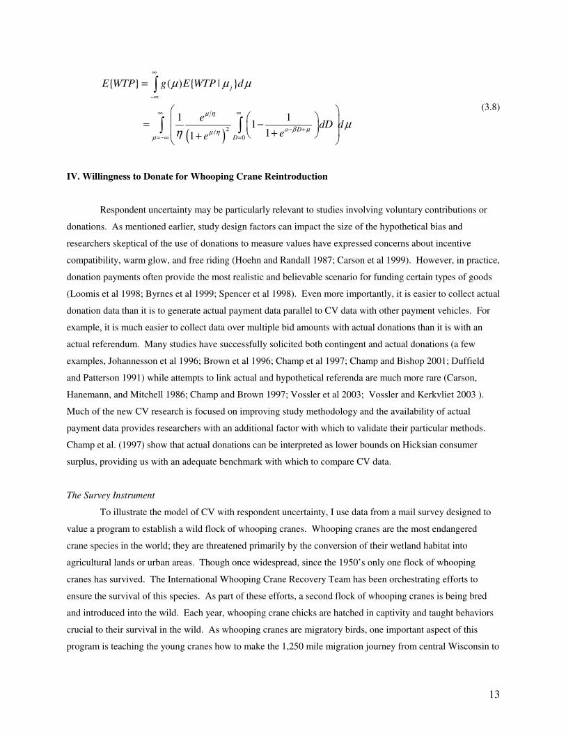
Rebecca Moore1

Job Market Paper

Agricultural and Applied Economics

University of Wisconsin 427 Lorch St., Madison, WI 53706

Rebeccamoore@wisc.edu

Abstract. One major critique of the contingent valuation (CV) method is that of “hypothetical bias”, named in

reference to the hypothetical market scenario intrinsic to the method. There are two noticeable shortcomings of the existing hypothetical bias literature: the absence of a utility-based model of respondent uncertainty and an insufficient number of studies that compare CV data that include uncertainty measures to actual payment data. I address both of these issues in this paper. I argue that hypothetical bias results, in part, from an invalid assumption of respondent certainty that is implicit in the conventional models of the CV decision. I develop a random utility based structural model that explicitly allows for respondent uncertainty. An application of this model to a study of actual and contingent donations to support a whooping crane reintroduction program shows that accounting for respondent uncertainty can significantly reduce hypothetical bias in a theoretically consistent manner.

1 I would like to express my sincere appreciation to Rich Bishop, Bill Provencher, and Patty Champ for their help with this research. This paper has benefited greatly from their many suggestions and inspiring discussions.

2

The United States federal government mandates the use of ex-ante cost-benefit analyses to evaluate all

major regulatory initiatives (Executive Order 12291 (1981); Executive order 12866 (1994)). To support this

mandate, the Office of Management and Budget (OMB) provides specific guidelines for conducting such

analyses (OMB 1992; OMB 2003). These guidelines state that benefits should reflect both use and non-use

values and should be measured based on the willingness to pay (WTP) principle. If market data for a good

exists, it should be used to estimate these benefits (OMB 2003). However, in the case of many environmental

and other public goods, a functioning market does not exist. For such non-market goods, the OMB guidelines

maintain that stated preference methods, including contingent valuation (CV), are appropriate for estimating

welfare benefits (OMB 2003). Possibly the most famous application of the CV method was its use in the

damage settlement related to the Exxon Valdez oil spill. The magnitude of the estimated non-use value of this

settlement was over $2.5 billion for the entire United States (Carson et al. 1992). This finding ignited a heated

debate among scholars and CV practitioners regarding the validity of the CV method (see for example

Diamond and Haussman 1994; Portney 1994; Hanemann 1994; NOAA 1993). While the intensity of the CV

debate has subsided in recent years, the method remains susceptible to criticism.

One major critique of the CV method is that responses to CV questions often generate higher

willingness to pay (WTP) estimates than comparable actual or simulated market data. This “hypothetical bias”

has been seen in studies valuing public goods and private goods, using both the willingness to pay and

willingness to accept principle, with different elicitation formats and different payment vehicles (List and

Gallet 2001; Little and Berrens 2003; Murphy et al 2005). Differences in study design can impact the size of

the hypothetical bias. For example, a meta-analysis by Little and Berrens (2003) found that the use of

referendum format can reduce the disparity between actual and hypothetical reported values, but their literature

review cited several referendum based studies in which the bias exists. Some of the current CV literature tests

various techniques to mitigate the bias, either by recoding the CV data or by adjusting the WTP estimates by

some calibration factor (for example Champ et al 1997; Brown et al. 2003; Vossler et al 2003; Norwood 2005).

This literature consists mainly of empirical experiments and meta-analyses without much focus on the

theoretical justification for the existence of the bias. This oversight has prevented researchers from adequately

motivating the various calibration techniques.

For example, a series of three experiments by Champ et al used a 10-point certainty scale on which

respondents indicated their certainty level regarding their answer to a dichotomous choice contingent donation

question (Champ et al 1997; Champ and Bishop 2001; Champ, Bishop, and Moore 2005). All three studies

found that the group of hypothetical “YES” respondents who were relatively certain they would make an

actual donation had similar attitudinal and demographic characteristics as the group of actual donors identified

from a parallel survey. The entire group of hypothetical “YES” respondents, including both the certain and

uncertain individuals, differed from the actual donors in these same characteristics. Their results suggest that

3

specific individuals who were uncertain of their CV response may be responsible for the apparent

discrepancies between contingent donations and actual donations. In effect, uncertain respondents are

providing incorrect responses to the dichotomous choice question by saying “YES” when there is a substantial

probability that they would say “NO” if actually asked to donate. Recoding the data from these uncertain

individuals, by assigning them a “NO” response, appears to reduce the hypothetical bias. However, the group

of certain respondents was defined differently in the different experiments. In one case, the certain

respondents were only those who circled ten on the scale (indicating the highest certainty level), but in the

other two studies, respondents circling an eight or nine were also considered certain. So while the recoding

method appears to reduce hypothetical bias, the lack of an underlying theoretical structure for dealing with the

uncertainty prevents the results from being readily transferable between studies.

In this paper, I contend that hypothetical bias exists not because the respondent provides an incorrect

(or hypothetical) answer to the CV question that must be corrected by the analyst, but rather because the

analyst misinterprets the correct answer by ignoring the respondent’s uncertainty. As part of their cost-benefit

analysis guidelines, the OMB outlines several principles that should be followed when designing and

conducting a CV study. One of these principles states that the “statistical and econometric methods used to

analyze the collected data be…well suited for the analysis, and applied with rigor and care” (OMB 2003, p.

23). I argue that the current analytical methods are based on invalid assumptions of respondent certainty and

thus are ill-suited for the CV problem. The assumption of respondent certainty leads to inflated estimates of

individual WTP and overstates the benefits of proposed regulation. To correctly interpret the data, it is

necessary to addresses respondent uncertainty pre-estimation, by incorporating it into the structural model. I

demonstrate that doing so will allow the analyst to more correctly estimate the value of the good being studied,

reducing the hypothetical bias and addressing a primary critique of the CV method.

I begin by presenting a structural model of the CV decision of an uncertain respondent, based on the

conventional random utility model first applied to CV by Hanemann (1985). The only other attempt to provide

a behavioral model of uncertainty based on a conventional CV model is that of Li and Mattsson (1995). Their

model is based on Cameron’s (1988) modeling approach that frames the decision in terms of the WTP function

directly. The Hanemann and Cameron approaches both identify the same decision (McConnell 1990), but one

advantage of the random utility framework is that it allows for the direct estimation of the preference

parameters. By incorporating the respondent’s uncertainty into this framework, the relationship between

preferences, utility, and WTP are made more transparent. A second limitation of the Li and Mattsson paper is

that it does not contain data from actual market transactions that could be compared to the results of the CV

analysis. Without such a comparison, the authors are unable to address the issue of hypothetical bias.

After outlining the decision of the uncertain respondent, I apply the model to data from a study of

actual and contingent donations for a whooping crane reintroduction project. Though true values for the

project cannot be observed (Bishop 2003), the availability of actual donation data provides a measure of

preferences that is independent of the contingent donations. Because the actual donation data reflects observed

4

market transactions, this data is arguably a better indicator of “true” preferences than are contingent donations.

A comparison between the two types of results is one way to test the criterion validity of CV (Boyle 2003;

Bishop 2003). To the best of my knowledge, this case study represents the first application of a theoretical

model of respondent uncertainty to both actual market observations and CV data. As such, it can begin to

address the criterion validity of the approach in a way that previous research could not. Three aspects of the

models are compared: the expected WTP values, the estimates of the preference parameters, and the

characteristics of the respondents answering “YES” to the dichotomous choice CV question. The results of

this case study support the conclusion that explicitly allowing for respondent uncertainty can significantly

reduce hypothetical bias in a theoretically consistent manner.

II. Respondent Uncertainty in the Contingent Valuation Literature

The idea of respondent uncertainty has been a relatively recent development in CV research, but has

generated a sizeable literature in this short time. This section provides a review of the existing literature most

relevant to this paper, but is not meant to represent the larger body of work regarding hypothetical bias and CV

methodology. Before getting into the literature, however, it is useful to think intuitively about the assumption

of respondent certainty in CV. Consider an individual who receives a CV survey in the mail. This individual,

Joe Public, reads about a possible change in some environmental good with which he may or may not already

be familiar. Then, Joe is asked whether or not he would agree to pay a certain amount of money to have this

good. Because this is a hypothetical scenario, Joe knows he will not actually have to pay, but he is asked to

answer as if it were a binding question. To assume respondent certainty is to assume that at the time he

answers the survey question, Joe Public has no doubt about how he would have responded if the survey had

involved a binding transaction in an actual market. In actuality, there is substantial empirical evidence to

suggest Joe is uncertain what his actual behavior would be.

Berrens et al (2002) identify two general methods of identifying respondent uncertainty: directly,

through the CV response, or indirectly, with a post-CV follow-up question. The direct approach is generally

found in studies employing a multiple-bounded question with polychotomous choices. For example, in a study

by Welsh and Poe (1998), individual respondents were presented with several bid amounts. For each bid, they

were asked to indicate whether or not they would vote for a proposal to reduce fluctuations in Glen Canyon

Dam releases if it were to cost the bid amount. The respondent answered “Definitely No”, “Probably No”,

“Not Sure”, “Probably Yes”, or “Definitely Yes” to each of the bid amounts. These categorical responses

allow the respondent to express uncertainty over at least some range of bids, but in this study the reported

uncertainty was not directly incorporated into the estimation of WTP. Instead, the responses were recoded into

“Yes/No” categories depending on the implied certainty level. One recoding included the “Definitely Yes”

responses as “Yes” and all other response options as a “No”. A second recoding included both the “Definitely

5

Yes” and “Probably Yes” responses as a “Yes” and the remaining categories as a “No”. The likelihood model

was estimated for each recoding and separate values of expected WTP were calculated.

Alberini, Boyle, and Welsh (2003) used a similar question to elicit anglers’ values of fishing. In this

study, most respondents marked each of the five response categories at least one time. This is strong evidence

that their respondents were uncertain about their answers. Like Welsh and Poe, these authors recoded the five

answer choices into “Yes/No” categories, but in an attempt to more explicitly incorporate respondent

uncertainty, they estimated a random effects probit model. In this model, respondent uncertainty can change

depending on the bid amount, which is consistent with the hypothesis that individuals are more uncertain about

their CV responses when asked about a bid amount relatively close to their true WTP. Other researchers have

questioned this approach, however, because of assumptions it requires regarding the independence of

responses across bid amounts for an individual respondent (Vossler and Poe 2005). Evans, Flores, and Boyle

(2003) suggest an alternative to the recoding method. Citing the results of cognitive research, they argue that

these verbal categories (e.g. “Definitely Yes”) should be interpreted as subjective probabilities. Doing so

avoids the need to recode the data, but requires the identification of a mapping from the uncertainty categories

into a probability value. Their results show similarities between this approach and the recoding approach used

by Welsh and Poe.

The other technique for identifying respondent uncertainty is with the use of a follow-up question to a

standard dichotomous choice CV question. The follow-up question asks respondents how certain they are of

the answer they provided to the CV question. The possible responses could be verbal categories, numerical

categories, or probabilities. In a study by Blumenschein et al (1998), respondents who said they would

purchase sunglasses at a particular price were asked if they were “Probably Sure” or “Definitely Sure” they

would actually pay that amount for the sunglasses. “Definitely sure” responses more accurately corresponded

to actual purchase decisions. The three experiments by Champ et al. discussed in the previous section used a

follow-up question with numerical categories in the form of a 10-point scale. All three experiments showed

that over 50% of the respondents were not entirely certain they would make an actual donation, despite having

said “YES” to the hypothetical dichotomous choice donation question. Loomis and Ekstrand (1998) also used

an ordinal 10-point scale to capture respondent uncertainty. They found that at extremely low and high bids,

respondents are more certain of their responses. Li and Mattsson (1995) framed their follow-up certainty

question in terms of probabilities, from 0 to 100%. Their paper presents a model in which uncertainty is

expressed in the WTP function by allowing the reported certainty probability to be correlated with the

probability that the individual’s WTP is greater or equal to the bid amount. A high reported certainty implies a

smaller variance of the unobserved component in the WTP function. Applying their uncertain respondent

model to data from a Swedish forest valuation survey, they found that the conventional model produced value

estimates six times larger the model adjusting for uncertainty. However, this paper does not have actual

market data with which to compare the contingent valuation responses and so the authors cannot relate this

difference to a systematic identification of those respondents responsible for the hypothetical bias.

6

A few studies have attempted to compare the different approaches for incorporating respondent

uncertainty into CV studies. For example, Ready, Navrud, and Dubourg (2001) compared polychotomous

choice (PC) responses to dichotomous choice (DC) with follow up certainty questions in a CV study valuing

health impacts from air pollution. The response categories for the follow up certainty question were verbal

categories with probability reference points given for the first and last category. For example, the survey

defined “Almost certain” as “95% sure” but “More likely” and “Equally likely” were not defined by actual

payment probabilities. They found that the DC responses indicated higher WTP values than the PC responses,

and that the PC respondents were more certain of their answers. When the DC data was recoded so that only

the “Almost certain/95% sure” responses were considered as a “YES”, the DC and PC responses were

statistically the same. They offer these results as evidence that DC respondents engage in “yea-saying”:

answering “yes” even if they are not very certain they would say yes in an actual payment scenario. In a

comparison of the two broad categories of certainty elicitation methods, Vossler et al (2003) compared the

results of a multiple bounded dichotomous choice survey and a survey with a single DC valuation question

with a follow up certainty question. Both surveys valued a green electricity program and the authors compared

various recoding methods for both elicitation formats. For example, a “Probably Yes” model of the multiple

bounded dichotomous choice data and a “Certainty >= 7” model of the follow up certainty data produce

similar estimates of mean WTP. In addition, the authors also have data on actual participation rates at a single

bid amount of $6. Hypothetical participation rates for these recoded models were similar to the actual

participation rates. However, a comparison of the entire WTP function estimated for these models shows

significant differences at other bid amounts. Unfortunately the actual participation data is only available at a

single offer amount, and so it is not possible to test criterion validity over a full range of offer amounts.

As a whole, these studies provide substantial empirical evidence of respondent uncertainty. In

addition, they suggest that this uncertainty is at least partially responsible for the hypothetical bias of the CV

method. However, there are two noticeable shortcomings of the existing literature: the absence of a utility-

based model of respondent uncertainty and an insufficient number of studies that compare CV data that include

uncertainty measures to actual payment data. I address both of these issues in this paper.

The Conventional Approach in Formal Terms

Hanemann’s (1985) original application of the random utility framework to dichotomous choice

contingent valuation (CV) data was an effort to formally explain the observations made by Bishop and

Heberlein (1979) in a study of individual’s willingness to sell a hunting permit. The model has since been

applied to a variety of goods, services, and payment mechanisms (see Boyle 2003 for more discussion on this).

This section provides a brief summary of the conventional random utility model applied to a willingness to pay

(WTP) question. Section 3 will relax some assumptions of this model in order to address the uncertainty issue.

Suppose an individual faces a standard dichotomous choice CV question, such as “Would you be

willing to pay $D in order to have …?”, where D is some specific dollar amount provided by the analyst. Let

7

Dj denote the offer amount seen by individual j, and CVj denote individual j’s “YES” or “NO” response to the

question. Individual utility is a linear function of income, y, and a random component, �, so that

( , )j j j j ju y yε α β ε= + + (2.1)

Faced with the CV question above, the individual will respond with a “YES” if the utility of a yes response is

greater than the utility of a no response, and a “NO” otherwise. The respondent knows his own value of �i, but

the analyst knows only the distribution of �j across the population, which is generally assumed to have an i.i.d.

Gumbel distribution with mean zero. Realized utility can be written as,

( ) ( )

0 00 1

1 1

1 0 1 0

(" " | ), ~

(" " | ) ( )

, with � ~ logistic(0,1)

no

yes

yes no

u no D u ywhere Gumbel

u yes D u y D

u u u D

D

α β εε ε

α β ε

α α β ε εα β ε

= = + + ���= = + − + ��

∆ = − = − − + −

= − +

(2.2)

The individual’s decision is deterministic in nature, but from the analyst’s perspective, the probability that CV

= “YES” for some offer amount D is given by,

( )

Pr( " " | ) Pr( 0)Pr( 0)

Pr ( )

11

1 D

CV YES D u

D

D

eα β

α β εε α β

−

= = ∆ ≥= − + ≥= ≥ − −

= −+

(2.3)

This is a standard logit model. Estimates of the utility parameters � and � are obtained and the estimated

model is then used to calculate welfare measures. In this paper, I focus on the expected willingness to pay,

E{WTP}, which is typically found by recognizing that WTP is itself a random variable. The probability that

WTP is greater than D is equal to one minus the probability of a “YES” response given in equation (2.3).

Hanemann showed that if WTP is restricted to be non-negative, E{WTP} can then be calculated as

( )0 0

1{ } Pr 1

1 DD

E WTP WTP D dD dDeα β

∞ ∞

−=

� �= > = −� �+ � � (2.4)

When the respondent is uncertain of her CV response, the conventional modeling approach is

inappropriate. Equations 2.2 and 2.4 assume that the respondent knows with certainty the utility of a “YES”

response and the utility of a “NO” response. In the following section, I present an alternative structural model

that takes advantage of the additional information provided by the individual faced with the following pair of

questions.

8

1. Would you be willing to pay $D in order to have…? 1 No 2 Yes

2. If you answered YES to question 1, on a scale of 1 to 10, where 1 means “very uncertain” and 10 means “very certain,” how certain are you that you would pay $D if you had an opportunity to actually do so?

1 2 3 4 5 6 7 8 9 10 very very

uncertain certain

As before, let CVj represent the response to the first question and Dj be the offer amount presented to

respondent j. Additionally, let Certj denote the number from 1 to 10 circled in the follow-up certainty

question. Unless Certj = 10 for all respondents who answer YES to the CV question, some respondents are

admittedly unsure what their behavior would be in an actual payment scenario, despite being able to answer

the hypothetical question presented. This directly contradicts the assumptions of the conventional model and

indicates respondents must be using some other decision rule to answer the CV question.

III. The uncertain respondent model

The individual respondent’s decision rule

There are many possible reasons why an individual would be uncertain about his response to a CV

question. Returning to our story of Joe Public, our average CV respondent, will illustrate this point. Joe may

have had little or no knowledge about the good in question prior to receiving the survey. When he reads the

CV question, Joe finds a dollar amount that he must consider on the spur of the moment. It would take time

and energy for Joe to sort through the information to identify his exact WTP. He might be unwilling to put the

same effort into answering a hypothetical question as he would when making an actual binding decision. It is

also possible that some of the factors affecting Joe’s WTP can only be realized when he is faced with an actual

monetary decision. For example, an individual’s discretionary income can vary from day to day. Joe might

have an average daily budget, but not know exactly what this budget will be on a particular day. An

unexpected expense (e.g. car repair or medical expense) could significantly lower his realized daily budget.

Alternatively, if Joe has recently received a monetary gift, he will have a higher daily income than expected. If

Joe considers his average daily budget when responding to the hypothetical scenario of a CV study, but some

realized value when faced with an actual scenario, it is not clear that the responses will be the same. In this

case, Joe is uncertain about his WTP and so he cannot be certain about his response to the CV question.

However, he is able to answer the question based on his expectations for what his WTP might be.

One way to formally model respondent uncertainty is to relax assumptions about the random

component of the utility function. Recall that in the conventional model the respondent knows �j with

certainty, but the analyst does not. The analyst treats �j as a random variable. To account for respondent

uncertainty, I assume the respondent in the hypothetical scenario does not know �j and so is unable to answer

9

the CV question with certainty. However, the individual does know the probability distribution of �j. From

this distribution, respondent j can calculate the probability that he would actually pay $D. This probability

depends on his expected value of �j, which he knows with certainty, and the bid amount, Dj. Assuming �j is

distributed logistically with mean �j and scale �, then the probability that individual j will make an actual

payment of D dollars, is given by

( ) /( )

1( , ) ( ; , ) 1

1 j jj

j j j j DD

p D f x dxe

α β µ σα β

µ µ σ∞

− +− −

= = −+

� (3.1)

where f is the logistic probability density function. A respondent faces the dichotomous choice CV question

with this actual payment probability in mind. He will answer “YES” if his actual payment probability is

sufficiently large, and “NO” otherwise. Let pmin represent the minimum actual payment probability needed to

provoke a “YES” response to a dichotomous choice question. Conceptualized in this way, a “YES” on the CV

question does not guarantee the individual would actually pay if faced with an actual payment scenario, only

that the probability of an actual payment is greater than pmin. At first glance, it might appear that pmin should

equal .5, so that a “YES” response reflects an actual payment probability of at least .5. However, it is also

possible that a “NO” response really means the actual payment probability is close to zero. In this case,

someone with only a small actual payment probability could answer “YES”. Rather than impose restrictive

assumptions, I treat pmin as a parameter to be estimated.

If pj represents individual j’s probability of an actual payment, then individual j will say “YES” to the

CV question if jp pmin≥ . Using equation (3.1), this condition will only hold if

ln1j j

pminD

pminα β µ σ � �

− + ≥ � �− (3.2)

The condition in (3.2) relates the respondent’s decision to his underlying utility function. Note that if pmin is

.5, the respondent will answer “YES” to the CV question if the expected utility of doing so is greater than the

expected utility of a “NO” response. The expectation operator is necessary because unlike the original

formulation, the respondent does not know �j with certainty.

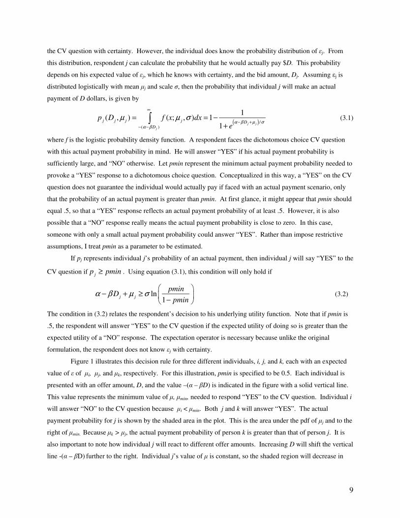
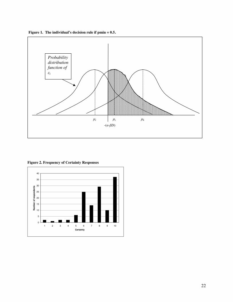
Figure 1 illustrates this decision rule for three different individuals, i, j, and k, each with an expected

value of � of �i, �j, and �k, respectively. For this illustration, pmin is specified to be 0.5. Each individual is

presented with an offer amount, D, and the value –(� – �D) is indicated in the figure with a solid vertical line.

This value represents the minimum value of �, �min, needed to respond “YES” to the CV question. Individual i

will answer “NO” to the CV question because �i < �min. Both j and k will answer “YES”. The actual

payment probability for j is shown by the shaded area in the plot. This is the area under the pdf of �j and to the

right of �min. Because �k > �j, the actual payment probability of person k is greater than that of person j. It is

also important to note how individual j will react to different offer amounts. Increasing D will shift the vertical

line -(� – �D) further to the right. Individual j’s value of � is constant, so the shaded region will decrease in

10

size. This is consistent with theory; an individual will be less likely to make an actual payment as the offer

amount increases.

A note on certainty scales and actual payment probabilities

With the benefit of hindsight, it is clear that the ideal response format for measuring respondent

uncertainty is to directly ask the respondent for actual payment probabilities. Few studies have used this

response format, however2, and for now, it is useful to consider how to incorporate other, more common,

response formats into the uncertain respondent model. These other response formats can be interpreted as

probabilities (Evans, Flores, and Boyle 2003). To do so, the analyst must specify the mapping of the

uncertainty data into actual payment probabilities. The case study I present in this paper contains uncertainty

data from a 10-point scale, as in the example question in the previous section. In this case, each value of the

scale represents a range of payment probabilities. For instance, if pmin = .5, the mapping could be that a “1”

on the certainty scale means the probability of an actual payment is between .5 and .55. A “2” on the certainty

scale means this probability is between .55 and .6, a “3” shows a probability between .6 and .65, and so on, so

that a “10” indicates a probability between .95 and 1. Note that in this example, a certainty of 1 maps into an

actual payment probability of at least pmin. This is a necessary condition for the individual to be answering

the certainty question at all. If the probability of an actual payment were less than pmin, CVj would be “NO”,

and the certainty question would be skipped. This example is a linear mapping in which each certainty level

represents a probability range of 0.05. This is only one of many possibilities and to avoid unnecessary

assumptions, the analyst can specify a general functional form for the mapping, and use the observed data to

estimate specific parameters. Let pl(cert) and ph(cert) represent the lower and upper bound on the actual

payment probability associated with certainty level cert. A general mapping of the certainty scale into

probabilities is

( )110

1

if cert = 1( )

( 1) if cert > 1

( ) ( ) , (1 )

lh

h l

i

pminp cert

p cert

p cert p cert k cert where k pmin iλ λ

−

=

�=

−�

� �= + ⋅ = − � � �

(3.3)

where � and pmin are estimable parameters, and k is a scaling term that ensures that ph(10) equals one. Note

that if � equals zero this mapping is equivalent to the linear mapping example above.

The choice of mapping is an empirical question, as the structural model is independent of the mapping

specification. For now, I assume only that all individuals answering “YES” to the CV question interpret the

certainty scale in the same manner. Answering “NO” to the CV question indicates the probability of an actual

payment is less than pmin. Ideally, further information about the “NO” respondents could come from a similar

type of certainty question, asking about the certainty of the “NO”. Such a question is difficult to ask in a clear 2 Li and Mattsson (1995) is one noted exception.

11

manner and raises concerns about individuals misinterpreting the question or the scale. Due to the lack of

additional information we can consider the bounds on the actual payment probability to be (-�, pmin) for all

“NO” respondents.

The analyst’s problem

From the respondent’s answer to the CV and follow up certainty questions, the analyst observes (or

infers) pjh, pj

l and Dj for each respondent and wants to estimate the preference parameters � and �. The analyst

does not observe �j, but based on the actual payment probability, the analyst can use equation (3.1) to infer

upper and lower bounds on the value, so that3,

( )" ", ln ,

1 ( )

sj js

j j jsj j

p DIf CV YES D for s l h

p Dµ α β

� �= = − + =� �� �−

(3.4)

The analyst does know the distribution of �j across the population, G(�). This is an additional element of

analyst uncertainty not present in the conventional model. With the conventional approach, everyone knows

their individual �j with certainty, so that E{�j} is just �j. The �j’s vary across the population, but the expected

value of �j in the population is assumed to be zero. Now it is the case that respondents themselves are

uncertain about �j and that the �j’s vary across the population.

Equation (3.4) presents the individual’s value of � as a function of observed data D, pl and ph, and

estimable utility parameters � and �. Given the values of these parameters and the population distribution of �,

the probability of the respondent’s observed response pattern (a “YES” on the CV question, followed by a

particular value on the certainty scale) is,

( )( ) ( )( )( )

Pr( " " | , , , , )

( ), ; , , , ( ), ; , , ,

Pr( " " | , , , , ) ln( ) ln(1 )

j j j

h h l lj j j j j j j j

j j j

CV YES and cert c D pmin

G p D D pmin G p D D pmin

CV NO D min G pmin pmin D

α β λ

µ α β λ µ α β λ

α β η α β

= = =

−

= = − − − +

(3.5)

These probabilities are the individual likelihood values. If we assume the population distribution of �j is

logistic with mean zero and a scale parameter �, the individual likelihood of j’s response is,

3 For the remainder of the paper, I assume the scale parameter of individual’s error distribution, �, is equal to 1 for identification reasons.

12

( )

( ) ( )( ) ( ) ( )( )

( ) ( ) ( )( )

ln ln 1 / ln ln 1 /

ln ln 1 /

, , , , ; , , | " "

1 1

1 11

, , , ; | " "1

h h l lj j j j j j

j

l hj j j j j

p p D p p D

j j j pmin pmin D

L pmin p p D CV YES

e e

L pmin D CV NOe

α β η α β η

α β η

α β η λ

α β η

− + − + − − + − + −

− + − + −

= =

−+ +

= =+

(3.6)

The likelihood value for the observed responses of all respondents is just the product of all likelihood values

indicated in (3.6). Maximum likelihood estimation can be used to obtain estimates for �, �, �, �, and pmin..

Calculating the Expected WTP

The uncertain respondent creates an additional dimension to the expectation of WTP. With the

conventional approach, the individual’s WTP is known with certainty by the individual. It is treated as a

random variable by the analyst who can not observe the individual’s �. The expectation operator used by the

analyst refers to the distribution of � across the population. In other words, E{WTP} is the WTP one would

expect an individual randomly selected from the population to possess.

When we allow respondents to have uncertainty regarding their own CV response, we are essentially

allowing them to be uncertain about their actual WTP (Li and Mattsson 1995). This leads us to two types of

expectations on WTP: the expected WTP of an individual and the expected WTP of the population. I will

refer to the individual’s expected WTP as E{WTP|�j}, the expected WTP conditional upon the individual’s

value of �. Conceptually, this is a different type of expectation than that of the conventional model, but it can

be calculated using a modified version of equation (2.4).

0 0

1{ | } Pr{ } 1

1 jj DD D

E WTP WTP D dD dDeα β µµ

∞ ∞

− += =

� �= > = −� �+ � � (3.7)

Equations (2.4) and (3.7) are both based on the relationship between an individual’s WTP and the probability

the individual will agree to make an actual payment of D. The difference is that in equation (3.7), this

probability is conditional on the individual’s value of �. Because we have restricted WTP to be nonnegative,

E{WTP|�j} is bounded below by zero, but as �j increases, the E{WTP|�j} will increase. Theoretically, this

formulation does not impose an upper bound on this conditional expectation. In practice, however, the

distribution of � is such that the probability of � being extremely large is negligible.

The second type of expectation, the population’s expected WTP, corresponds directly to the

expectation operator in the conventional model and so we denote this value as E{WTP}. Individuals know

their own value of �, but the analyst does not. There is a distribution of � across the population, and the

E{WTP} is the WTP one would expect an individual randomly selected from the population to possess. This

is the unconditional E{WTP} because it is unconditional upon the individual’s �j. If g(�) represents the

logistic p.d.f. of � across the population, invoking the Theorem of Total Expectations (Greene 2003) gives us

an expression for E{WTP},

13

( )2/0

{ } ( ) { | }

1 11

11

j

a DD

E WTP g E WTP d

edD d

ee

µ η

β µµ ηµ

µ µ µ

µη

∞

−∞

∞ ∞

− +=−∞ =

=

� �� �� �= −� �� �+ +

�

� �

(3.8)

IV. Willingness to Donate for Whooping Crane Reintroduction

Respondent uncertainty may be particularly relevant to studies involving voluntary contributions or

donations. As mentioned earlier, study design factors can impact the size of the hypothetical bias and

researchers skeptical of the use of donations to measure values have expressed concerns about incentive

compatibility, warm glow, and free riding (Hoehn and Randall 1987; Carson et al 1999). However, in practice,

donation payments often provide the most realistic and believable scenario for funding certain types of goods

(Loomis et al 1998; Byrnes et al 1999; Spencer et al 1998). Even more importantly, it is easier to collect actual

donation data than it is to generate actual payment data parallel to CV data with other payment vehicles. For

example, it is much easier to collect data over multiple bid amounts with actual donations than it is with an

actual referendum. Many studies have successfully solicited both contingent and actual donations (a few

examples, Johannesson et al 1996; Brown et al 1996; Champ et al 1997; Champ and Bishop 2001; Duffield

and Patterson 1991) while attempts to link actual and hypothetical referenda are much more rare (Carson,

Hanemann, and Mitchell 1986; Champ and Brown 1997; Vossler et al 2003; Vossler and Kerkvliet 2003 ).

Much of the new CV research is focused on improving study methodology and the availability of actual

payment data provides researchers with an additional factor with which to validate their particular methods.

Champ et al. (1997) show that actual donations can be interpreted as lower bounds on Hicksian consumer

surplus, providing us with an adequate benchmark with which to compare CV data.

The Survey Instrument

To illustrate the model of CV with respondent uncertainty, I use data from a mail survey designed to

value a program to establish a wild flock of whooping cranes. Whooping cranes are the most endangered

crane species in the world; they are threatened primarily by the conversion of their wetland habitat into

agricultural lands or urban areas. Though once widespread, since the 1950’s only one flock of whooping

cranes has survived. The International Whooping Crane Recovery Team has been orchestrating efforts to

ensure the survival of this species. As part of these efforts, a second flock of whooping cranes is being bred

and introduced into the wild. Each year, whooping crane chicks are hatched in captivity and taught behaviors

crucial to their survival in the wild. As whooping cranes are migratory birds, one important aspect of this

program is teaching the young cranes how to make the 1,250 mile migration journey from central Wisconsin to

14

Florida. After being led to Florida by an ultralight aircraft their first year, the cranes are able to make the

return trip to Wisconsin unassisted the next spring. They will also continue the migration annually as a flock,

without the assistance of an aircraft. However, to enhance the chances of success of the program, radio

transmitters are placed on the leg of each crane to monitor the birds’ locations during migration and throughout

the year. If a bird is in danger or sick, scientists will intervene and rescue the bird. The first class of cranes, 18

birds, was hatched in the spring of 2001. The project will continue until the flock has grown to 125 cranes

(approximately 10-15 years). At the time of the study, funding was needed to purchase radio transmitters for

whooping crane chicks who were to be hatched in the spring of 2004. The transmitters cost around $300 each,

and while survey respondents were not told the cost of the transmitters, they were told that the transmitters

could only be provided if there was sufficient support in the form of donations.

The survey sample contained two treatment groups4. Both groups were presented with identical

descriptions of the whooping crane reintroduction project. Following this description, one group was asked a

dichotomous choice contingent donation (CD) question and a follow up certainty question similar to the

example given in Section 2. The other group was asked a similar dichotomous choice question, except that an

actual donation (AD) would be required. That is, for this group, respondents answering “YES” to the donation

question were asked to include a check for the bid amount when they returned their survey. A total of $1510

in donations was collected from this group. Table 1 presents the sample sizes, response rates, and percentages

of respondents answering “YES” to the donation question for each offer amount in both treatments. In this

case study, we analyze the survey data with both the conventional model and my model of respondent

uncertainty. As an additional point of comparison, we will also present the results from estimating the

conventional model with one set of “recoded” CD data. The “CD8” data considers all hypothetical donors

who circled 8, 9 or 10 on the certainty scale as “YES” respondents, and all others as “NO” respondents. This

particular recoding was previously identified as the most appropriate for this data set (Champ, Bishop, and

Moore 2005). The final column of Table 1 indicates the percentage of “YES” respondents identified by this

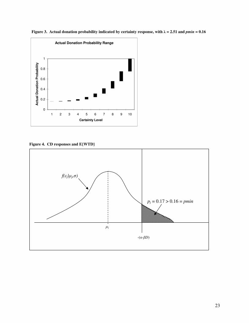
recoded data. Figure 2 shows the frequency of responses to the follow-up certainty question. Though the most

common response was 10, the median certainty level was only 8, indicating over half of the “YES”

respondents were uncertain of their answer choice and highlighting the need for a modeling approach that

incorporates this uncertainty. The mean certainty was 7.72.

Estimating the Conventional and Uncertain Respondent Models

4 There were actually three treatments in this survey. One group was given a contingent donation question preceded by a “cheap talk” script and is irrelevant to the current paper. Details of this aspect of the survey can be found in Champ, Bishop, and Moore (2005).

15

The first three columns of Table 2 report parameter estimates and standard errors of the utility

parameters � and � and a point estimate of the expected willingness to pay (E{WTP})5 as derived from

equation (2.4). Several techniques are available to estimate the distribution of E{WTP} (Kling 1991; Cooper

1994). For this study I relied on the Krinsky and Robb procedure adapted to non-market valuation by Park,

Loomis, and Creel (1991) to estimate a 90% confidence interval for E{WTP}. These results clearly show a

hypothetical bias in the data. The expected WTP of the contingent donation group ($69.38) is over three times

larger than that of the actual donation group ($21.21). Table 2 also shows the results of estimating the

conventional model with the recoded CD data. The recoding successfully lowers the E{WTP} estimate to

values not significantly different from the actual donation results.

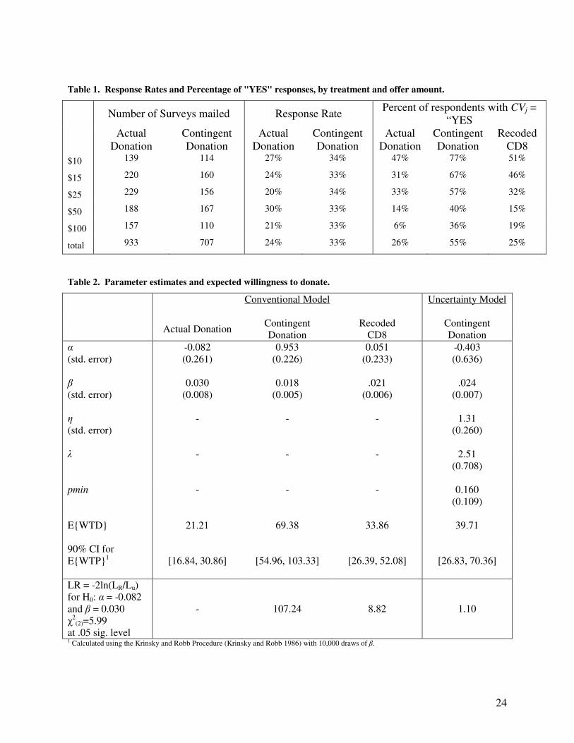
The final column of Table 2 reports the parameter estimates and E{WTD} estimate generated with the

uncertain respondent model. This model includes three additional parameters: � is the scale parameter for the

population’s distribution of �, � is a parameter in the mapping of uncertainty into probability, and pmin is the

minimum actual payment probability needed to generate a “YES” response to the dichotomous choice

contingent donation question. Given the estimates of � and pmin, the mapping of the certainty scale into

payment probabilities (equation (3.3)) is fully identified. Figure 3 graphically depicts this mapping. Note that

with these parameter values, lower certainty values map into smaller probability ranges. A certainty of “5”

represents a payment probability between .20 and .25, but a certainty of “10” represents a probability range

from .75 to 1.

Comparing the Estimation Results

Several interesting conclusions can be drawn from the results in Table 2. First, we can examine the

E{WTP} values inferred from each model. The recoding method produced a lower E{WTP} than the straight

forward CD model, and the confidence interval of the CD8 and AD models overlap. These results are

consistent with previous studies (Champ and Bishop 2001, Champ et al 1997). The uncertain respondent

model generated an E{WTP} between that of the contingent donation and actual donation results. This is

intuitive, considering that the estimated value of pmin is well below .5. This result clearly suggests that

individuals are answering “YES” to the dichotomous choice question, even though they are not expected to

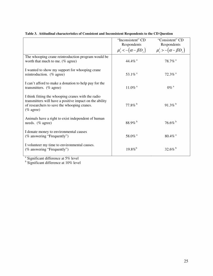
make an actual donation. This idea is illustrated in Figure 4. Individual j is presented with a hypothetical

donation question with bid amount Dj. Because his value of pj is .17, which is greater than pmin, this

individual will answer “YES” to the CD question. The conventional model equates a “YES” response to the

CD question as an indication that �j is greater than -(� – �D). With the uncertain respondent model,

individual j’s expected value of � could be less than -(� – �D), and yet the individual will give a “YES”

response to the CD question. In fact, all respondents whose value of � lies between �j and -(� – �D) have a

5 To be exact, in this case study I am estimating the expected willingness to donate (WTD), which is a lower bound on the expected willingness to pay (Champ and Bishop 2001). To avoid introducing unnecessary confusion between WTP and WTD, in this paper, I refer to both as WTP.

16

conditional E{WTP|�} less than the offer amount, D, but will respond “YES” to the CD question. Our results

imply that explicitly allowing for this type of “inconsistent” response will produce an E{WTP} estimate closer

to that implied by the actual donation data, reducing the hypothetical bias.

Simply comparing the E{WTP} values generated by each model does not provide sufficient proof that

one model is better than the other. However, our model of uncertain respondents is based on the random

utility framework and so provides estimates of the underlying utility parameters � and �. Because the actual

donation and contingent donation decisions are based on the same underlying utility function, the preference

parameters estimated with the CD data should be identical to the “true” values provided by the actual donation

data. Typically, this is tested by pooling the hypothetical and actual data, estimating the parameters of the

pooled model, and calculating a likelihood ratio statistic comparing the likelihood values of the pooled

regression (the restricted model) and the separate regressions (the unrestricted model). If the hypothesis is

rejected, this indicates the actual and hypothetical donation data are generated from two different utility

functions. Because the model of the uncertain respondent includes additional probability data not present in

the actual donation data, the data cannot be pooled without imposing some assumptions about the actual

donors. In addition, it is not possible to restrict � in such a way that the uncertain respondent model is

equivalent to the conventional model. In other words, the conventional model and the uncertain respondent

model are non-nested and I cannot perform a likelihood-ratio test. Instead, I propose an alternative, but

similar, hypothesis. If we take the point estimates of the utility parameters from the actual donation model as

the “true” values, we can test the null hypothesis that our model identifies the true utility parameters, H0: � =

�actual and � = �actual, where the subscript “actual” refers to the point estimates of the actual donation model.

For consistency, I use a LR statistic to test this hypothesis for both the conventional and the uncertainty

models. The results show that utility parameters estimated with the uncertain respondent model are

statistically indistinguishable from the true parameter values identified with the actual donation data, but the

other models identified different parameters. Unlike the conventional model, the uncertain respondent model

allows the random component of the utility function to be structurally different in the actual and hypothetical

decision process and this allows the analyst to recover the identical parameters for the deterministic component

of utility.

So far in the discussion, I have not considered the impact of covariates in the decision model, although

they can significantly increase the predictive power of the model (Haab and McConnel 2003). The inclusion

of additional explanatory variables is straight forward in both the conventional and uncertain respondent

model; these variables enter as part of the deterministic portion of the utility function. E{WTP} estimates are

then conditional on particular values of these additional variables (Haab and McConnell 2003). For this study,

we are not particularly concerned with the impact of these variables on E{WTP}, but it is still instructive to

look at the additional information these variables provide. It is particularly enlightening to divide the

respondents answering “YES” to the CD question into two groups; those whose would be expected to make a

donation if actually asked to do so and those who would not. We label the first group the “Consistent”

17

respondents, because their CD responses are consistent with their expected AD responses. This is the group of

individuals whose conditional E{WTP|�} is greater than the bid amount. In other words, their values of � are

greater than -(� – �D). The other group contains the “Inconsistent” respondents, whose E{WTP|�} < D, but

still answer “YES” to the CD question. Table 3 compares the reported attitudes of the individuals in these two

groups. As might be expected, the consistent respondents report a greater desire to support the whooping crane

reintroduction project specifically (“The whooping crane program would be worth that much to me”), while

the inconsistent respondents are more likely to value broader environmental ideals (“Animals have a right to

exist”). The consistent respondents are also more likely to have donated time or money to environmental

causes in the past, providing them with additional experience on which to base their expectation.

V. Discussion and Concluding Remarks

The results of the case study suggest that explicitly incorporating respondent uncertainty into the

estimation model can generate E{WTP} values and utility parameter estimates consistent with actual donation

data. The results also support the conclusions of previous studies that have suggested there are certain

individuals responsible for the apparent hypothetical bias of CV data. Although some would accuse these

individuals of providing “false positives”, in actuality, it is the analyst who is misinterpreting the respondent’s

answers. Further research is needed before definitive conclusions can be reached regarding the performance of

this model of respondent uncertainty. In designing future studies, it will be useful to consider two important

assumptions that I made in this application.

The first assumption is the mapping of the certainty scale into probabilities. I specified a parametric

form for this mapping, and used maximum likelihood estimation to find estimates of both the mapping

parameters and the preference parameters. The results indicate that uncertain respondents are likely to say

“YES” to a dichotomous choice contingent donation question even if they do not expect to make an actual

donation. This is consistent with previous studies, however it is unclear how robust this result would be to

changes in either the good or the payment vehicle and further investigation is needed to explore this issue. One

potential method of avoiding this problem altogether would be to ask respondents for their actual payment

probability directly, instead of trying to infer this information from a certainty scale. This would eliminate the

need to ask the dichotomous choice question and readily transfer between studies. Several researchers have

pushed for this idea, but the published literature has not yet reflected this mandate (Manski 2005; Ready and

Navrud 2001).

The second assumption that needs further exploration is the distribution of � across the population. I

assumed � to be distributed logistically around zero. This implies that the expected value of � across the

population is also zero. For identification, the location parameter of the distribution must equal zero, but a

skewed distribution of � would result is a non-zero expected �. A truncated distribution of � could be used to

impose restrictions on the range of WTP. With a donation payment vehicle, it is reasonable to assume that

18

WTP is bounded below by zero and above by income. Imposing this restriction post-estimation is acceptable

in certain cases, but it would be better to impose the restriction in the estimation itself. Methods of imposing

bounds in the estimation of the conventional model have been suggested, but these modes are complex and not

always well behaved (Haab and McConnell 2003). The added dimension of the � parameter in our formulation

of respondent uncertainty could provide a simpler way of imposing these bounds.

This paper provides an alternative approach to modeling the decision of the uncertain respondent in a

contingent valuation study. These results suggest a starting point for future CV research. Applications of this

and possibly other theoretical models of respondent uncertainty are needed before any conclusions can be

drawn regarding the link between uncertainty and hypothetical bias. Particularly, applications involving other

types of goods, different elicitation methods, and different payment vehicles are needed. This paper also

echoes the need to frame CV responses in terms of actual payment probabilities. Doing so would significantly

reduce the number of analyst imposed assumptions needed to interpret the results. It is important to continue

to improve the current methods of collecting and analyzing CV studies due to their potentially large role in

cost-benefit analysis, a decision-making tool used frequency by both public and private groups.

VI. References Alberini, A., K. Boyle, and M. Welsh (2003) “Analysis of Contingent Valuation Data with Multiple Bids and Response Options Allowing Respondents to Express Uncertainty,” Journal of Environmental Economics and Management 45(1): 40-62. Berrens, R.P., H. Jenkins-Smith, A. K. B., and C.L. Silva (2002) “Further Investigation of Voluntary Contribution Contingent Valuation: Fair Share, Time of Contribution, and Respondent Uncertainty.” Journal of Environmental Economics and Management 44(1): 144-168. Bishop, R.C. and T.A. Heberlein (1979) “Measuring Values of Extra-Market Goods: Are Indirect Measures Biased?” American Journal of Agricultural Economics 61(5): 926-930. Bishop, R. C. (2003). “Where To From Here?” In A Primer on Non-Market Valuation, edited by Patricia A. Champ, Kevin J. Boyle, and Thomas C. Brown. Boston: Kluwer Academic Publishers. Blumenschein, K., M. Johannesson, G.C. Blomquist, B. Liljas, and R.M. O’Conor (1998) “Experimental Results on Expressed Certainty and Hypothetical Bias in Contingent Valuation.” Southern Economic Journal 65(1): 169-177. Boyle, K.J. (2003). “Contingent Valuation in Practice.” In A Primer on Non-Market Valuation, edited by P.A. Champ, K.J. Boyle, and T.C. Brown. Boston: Kluwer Academic Publishers. Brown, T.C., I. Ajzen, and D. Hrubes (2003) “Further tests of entreaties to avoid hypothetical bias in referendum contingent valuation” Journal of Environmental Economics and Management 46: 353-361. Byrnes, B., C. Jones, and S. Goodman (1999) “Contingent Valuation and Real Economic Commitments: Evidence from Electric Utility Green Pricing Programmes.” Journal of Environmental Planning and Management 42(2): 149-166.

19

Cameron, T.A. (1988) “A New Paradigm for Valuing Non-Market Goods Using Referendum Data: Maximum Likelihood Estimation by Censored Logistic Regression” Journal of Environmental Economics and Management 15(3): 35-379. Carson, R.T., W.M. Hanemann, R.C. Mitchell (1986) “The Use of Simulated Political Markets to Value Public Goods” Economics Department, University of California, San Diego. Carson, R.T., R.C. Mitchell, W. M. Hanemann, R.J. Kopp, S. Presser, and P.A. Ruud (1992). A Contingent Valuation Study of Lost Passive Use Values Resulting from the Exxon Valdez Oil Spill. Report to the Attorney General of the State of Alaska, La Jolla, CA: Natural Resource Damage Assessment (NRDA), Inc. Carson, R., R. Groves, and M. Machina (1999) “Incentive and Informational Properties of Preference Questions.” Plenary Address, European Association of Resource and Environmental Economists, Oslo, Norway. Champ, P.A., R.C. Bishop, T.C. Brown, and D.W. McCollum (1997) “Using Donation Mechanisms to Value Nonuse Benefits from Public Goods” Journal of Environmental Economics and Management 33(2): 151-162. Champ, P.A. and T.C. Brown (1997) “A comparison of Contingent and Actual Voting Behavior.” Proceedings from W-133 Benefits and Cost Transfer in Natural Resource Planning, 10th Interim Report. Champ, Patricia A. and Richard C. Bishop (2001) "Donation Payment Mechanisms and Contingent Valuation: An Empirical Study of Hypothetical Bias." Environmental and Resource Economics 19: 383-402. Champ, P.A., R.C. Bishop, and R. Moore (2005) “Approaches to Mitigating Hypothetical Bias.” Proceedings from 2005 Western Regional Research Project W-1133: Benefits and Costs in Natural Resource Planning, Salt Lake City, UT. Cooper, J.C. (1994) “A Comparison of Approaches to Calculating Confidence Intervals for Benefit Measures from Dichotomous-Choice Contingent Valuation Surveys.” Land Economics 70(1): 111-122. Diamond, P.A., and J.A. Hausman (1993). “Contingent Valuation: Is Some Number Better Than No Number?” Journal of Economic Perspectives 8(4): 455-464. Evans, M.F., N.E. Flores, and K.J. Boyle (2003) “Multiple-Bounded Uncertainty Choice Data as Probabilistic Intentions” Land Economics 79(4): 549-560. Greene, W.H. (2003) Econometric Analysis, Fifth Edition. Upper River, New Jersey: Prentice Hall. Haab, T.C. and K.E. McConnel (2003) Valuing Environmental and Natural Resources: The Econometrics of Non-Market Valuation. Northhampton, MA: Edward Elgar. Hanemann, W. M. (1984) “Welfare Evaluations in Contingent Valuation Experiments with Discrete Responses” American Journal of Agricultural Economic 66(3): 332-341. Hanemann, W. M. (1994) “Valuing the Environment Through Contingent Valuation.” Journal of Economic Perspectives 8(4): 19-43. Hoehn, J. and A. Randall (1987) “A Satisfactory Benefit Cost Indicator from Contingent Valuation.” Journal of Environmental Economics and Management 14: 226-247. Kling, C.L. (1991) “Estimating the Precision of Welfare Measures.” Journal of Environmental Economics and Management 21(3): 244-259.

20

Li, C. Z., and L. Mattsson (1995) “Discrete Choice Under Preference Uncertainty: An Improved Structural Model for Contingent Valuation” Journal of Environmental Economics and Management 28(2): 256-269. List, J. A. and C. A. Gallet (2001). "What Experimental Protocol Influences Disparities Between Actual and Hypothetical Stated Values?" Environmental and Resource Economics 20: 241-254. Little, J. and R. Berrens (2003). "Explaining Disparities between Actual and Hypothetical Stated Values: Further Investigation Using Meta-Analysis." Economics Bulletin 3(6): 1-13. Loomis, J. and E. Ekstrand, “Alternative Approaches for Incorporating Respondent Uncertainty When Estimating Willingness to Pay: The Case of the Mexican Spotted Owl.” Ecological Economics 27(1): 29-41. McConnell, K. E. (1990) “Models for Referendum Data: The Structure of Discrete Choice Models for Contingent Valuation” Journal of Environmental Economics and Management 18(1): 19-34. Murphy, J.J., G.P. Allen, and T.H. Stevens (2005) “A Meta-analysis of Hypothetical Bias in Sated Preference Valuation.” Environmental and Resource Economics 30(3): 313-325. National Oceanic and Atmospheric Administration (NOAA) (1993). Natural Resource Damage Assessments under the Oil Pollution Act of 1990. Federal Register 58 (January 15, 1993) 4601. Norwood, F. B. (2005) “Can Calibration Reconcile Stated and Observed Preferences?” Journal of Agricultural and Applied Economics 37(1): 237-48. Office of Management and Budget (OMB) (1992). “Guidelines and Discount Rates for Benefit-Cost Analysis of Federal Programs.” Circular A-94, October 29, 1992. Office of Management and Budget (OMB) (2003). “Regulatory Analysis.” Circular A-4, September 17, 2003. Park, T., J. Loomis, and M. Creel (1991) “Confidence Intervals for Evaluating Benefit Estimates from Dichotomous Choice Contingent Valuation Studies.” Land Economics67(1): 64-73. Portney, P.R. “The Contingent Valuation Debate: Why Economists Should Care” Journal of Economic Perspectives 8(4): 3-17. President (1981). “Federal Regulation, Executive order 12291.” Federal Register 46 (February 19, 1981): 13193. President (1993). “Regulatory Planning and Review, Executive order 12866.” Federal Register 58 (September 30, 1993): 51735-51744. Ready, R.,S. Navrud, and W.R. Dubourg (2001) “How Do Respondents with Uncertain Willingness to Pay Answer Contingent Valuation Questions?” Land Economics 77(3):315-326. Spencer, M. A., S.K. Swallow, and C.J. Miller (1998) “Valuing Water Quality Monitoring: A Contingent Valuation Experiment Involving Hypothetical and Real Payments.” Agricultural and Resource Economic Review 27(1): 23-42. Vossler, C.A., R.G. Ethier, G.L. Poe, and M.P. Welsh (2003) “Payment Certainty in Discrete Choice Contingent Valuation Responses: Results from a Field Validity Test” Southern Economic Journal 69(4): 886-902.

21

Vossler, C.A., J. Kerkvliet, S. Polasky, O.Gainutdinova (2003) “Externally Validating Contingent Valuation: An Open-Space Survey and Referendum in Corvallis, Oregon.” Journal of Economic Behavior and Organization 51(2): 261-277. Vossler, C.A. and J. Kerkvliet (2003) “A Criterion Validity Test of the Contingent Valuation Method: Comparing Hypothetical and Actual Voting Behavior for a Public Referendum.” Journal of Environmental Economics and Management 45(3) 631-649. Vossler, C.A. and G.L. Poe (2005) “Analysis of Contingent Valuation Data with Multiple Bids and Response Options Allowing Respondents to Express Uncertainty: A Comment,” Journal of Environmental Economics and Management 49(1): 197-200. Welsh, M.P., and G.L. Poe (1998) “Elicitation Effects in Contingent Valuation: Comparisons to a Multiple Bounded Discrete Choice Approach.” Journal of Environmental Economics and Management 36(2): 170-185.

22

Figure 1. The individual’s decision rule if pmin = 0.5.

Figure 2. Frequency of Certainty Responses

0

5

10

15

20

25

30

35

40

1 2 3 4 5 6 7 8 9 10

Certainty

Num

ber

of r

espo

nden

ts

�j �i

-(�-�D)

�k

Probability distribution function of �i

23

Figure 3. Actual donation probability indicated by certainty response, with � = 2.51 and pmin = 0.16

Actual Donation Probability Range

0

0.2

0.4

0.6

0.8

1

1 2 3 4 5 6 7 8 9 10

Certainty Level

Act

ual D

onat

ion

Pro

babi

lity

Figure 4. CD responses and E{WTD}

�j

-(�-�D)

pj = 0.17 > 0.16 = pmin

f(�j|�j,�)

24

Table 1. Response Rates and Percentage of "YES" responses, by treatment and offer amount.

Number of Surveys mailed Response Rate Percent of respondents with CVj = “YES

Actual

Donation Contingent Donation

Actual Donation

Contingent Donation

Actual Donation

Contingent Donation

Recoded CD8

$10 139 114 27% 34% 47% 77% 51%

$15 220 160 24% 33% 31% 67% 46%

$25 229 156 20% 34% 33% 57% 32%

$50 188 167 30% 33% 14% 40% 15%

$100 157 110 21% 33% 6% 36% 19%

total 933 707 24% 33% 26% 55% 25%

Table 2. Parameter estimates and expected willingness to donate.

Conventional Model Uncertainty Model

Actual Donation Contingent Donation

Recoded CD8

Contingent Donation

� (std. error)

-0.082 (0.261)

0.953 (0.226)

0.051 (0.233)

-0.403 (0.636)

� (std. error)

0.030 (0.008)

0.018 (0.005)

.021 (0.006)

.024 (0.007)

� (std. error)

- - - 1.31 (0.260)

�

- - - 2.51 (0.708)

pmin

- - - 0.160 (0.109)

E{WTD}

21.21 69.38 33.86 39.71

90% CI for E{WTP}1

[16.84, 30.86] [54.96, 103.33] [26.39, 52.08] [26.83, 70.36]

LR = -2ln(LR/Lu) for H0: � = -0.082

and � = 0.030 �

2(2)=5.99

at .05 sig. level

- 107.24 8.82 1.10

1 Calculated using the Krinsky and Robb Procedure (Krinsky and Robb 1986) with 10,000 draws of �.

25

Table 3. Attitudinal characteristics of Consistent and Inconsistent Respondents to the CD Question

“Inconsistent” CD Respondents

( )lj jDµ α β< − −

“Consistent” CD Respondents

( )lj jDµ α β> − −

The whooping crane reintroduction program would be worth that much to me. (% agree)

44.4% a 78.7% a

I wanted to show my support for whooping crane reintroduction. (% agree)

53.1% a 72.3% a

I can’t afford to make a donation to help pay for the transmitters. (% agree)

11.0% a 0% a

I think fitting the whooping cranes with the radio transmitters will have a positive impact on the ability of researchers to save the whooping cranes.

(% agree)

77.8% b 91.3% b

Animals have a right to exist independent of human needs. (% agree)

88.9% b 76.6% b

I donate money to environmental causes (% answering “Frequently”)

58.0% a 80.4% a

I volunteer my time to environmental causes. (% answering “Frequently”)

19.8%b 32.6% b

a Significant difference at 5% level b Significant difference at 10% level